ANY OPINIONS EXPRESSED ARE THOSE OF THE AUTHOR(S) AND NOT NECESSARILY THOSE OF THE SCHOOL OF ECONOMICS & SOCIAL SCIENCES, SMU

External Debt, Adjustment, and Growth (This is a revised version of an earlier SMU Economics and Statistics Working Paper #07-2005)

Roberto S. Mariano, Delano Villanueva May 2006

Paper No. 13-2006

SSSMMMUUU EEECCCOOONNNOOOMMMIIICCCSSS &&& SSSTTTAAATTTIIISSSTTTIIICCCSSS WWWOOORRRKKKIIINNNGGG PPPAAAPPPEEERRR SSSEEERRRIIIEEESSS

External Debt, Adjustment, and Growth

By Roberto Mariano and Delano Villanueva§

Singapore Management University

High ratios of external debt to GDP in selected Asian countries have contributed

to the initiation, propagation, and severity of the financial and economic crises in recent

years, reflecting runaway fiscal deficits and excessive foreign borrowing by the private

sector. More importantly, the servicing of large debt stocks has diverted scarce resources

from investment and long-term growth.

Applying and calibrating the formal framework proposed by Villanueva (2003) to

Philippine data, we explore the joint dynamics of external debt, capital accumulation, and

growth. The relative simplicity of the model makes it convenient to analyze the links

between domestic adjustment policies, foreign borrowing, and growth. We estimate the

optimal domestic saving rate that is consistent with maximum real consumption per unit

of effective labor in the long run. As a by-product, we estimate the steady-state ratio of

net external debt to GDP that is associated with this optimal outcome. The framework is

an extension of the standard neoclassical growth model that incorporates endogenous

technical change and global capital markets. The major policy implications are that in

the long run, fiscal adjustment and the promotion of private saving are critical; reliance

on foreign saving in a globalized financial world has limits; and when risk spreads are

highly and positively correlated with rising external debt levels, unabated foreign

borrowing depresses long run welfare. JEL F34, F43, O41

_____________________________________________________________________ §Roberto S. Mariano is Vice-Provost for Research and Dean of the School of Economics and

Social Sciences at Singapore Management University. Delano P. Villanueva is Visiting Professor, School

of Economics and Social Sciences, Singapore Management University, and former Advisor, IMF Institute

and Research Director, South East Asian Central Banks (SEACEN) Research and Training Centre.

We would like to thank, without implicating, Thorvaldur Gylfason, Partha Sen, and Sunil Sharma

for useful comments, David Fernandez and Fee Ying Tan of JP Morgan, Singapore for providing the data

on spreads, Bangko Sentral ng Pilipinas’ Governor Amando Tetangco, Jr. and members of the Monetary

Board for a stimulating discussion, Assistant Governor Diwa Guinigundo and his staff for Philippine

macroeconomic data and valuable inputs, discussants at the NBER/EASE 16 Conference in Manila during

June 23-25, 2005 for helpful suggestions, and Choon Yann Leow for excellent research assistance.

2

Contents

I. Introduction

II. The Formal Framework

III. Application to the Philippines

IV. Implications for Fiscal Policy and External Debt Management

V. Conclusion

Appendix A: Stability Analysis

Appendix B: Data

References

3

I. Introduction

High ratios of external debt to GDP in selected Asian countries have contributed

to the initiation, propagation, and severity of the financial and economic crises in recent

years, reflecting runaway fiscal deficits and excessive foreign borrowing by the private

sector. More importantly, the servicing of large debt stocks has diverted scarce resources

from investment and long-term growth. Applying and calibrating the formal framework

proposed by Villanueva (2003) to Philippine data, we explore the joint dynamics of

external debt, capital accumulation, and growth. The relative simplicity of the model

makes it convenient to analyze the links between domestic adjustment policies, foreign

borrowing, and growth. We estimate the optimal domestic saving rate that is consistent

with maximum real consumption per unit of effective labor in the long run. As a by-

product, we estimate the steady-state ratio of net external debt to GDP that is associated

with this optimal outcome.

The framework is an extension of the standard neoclassical growth model that

incorporates endogenous technical change and global capital markets. The steady-state

ratio of the stock of net external debt to GDP is derived as a function of the real world

interest rate, the spread and its responsiveness to the external debt burden and market

perception of country risk, the propensity to save out of gross national disposable income,

rates of technical change, and parameters of the production function.1

1 Being concerned primarily with the long-run interaction between external debt, growth, and adjustment, our non-stochastic paper is not about solvency or liquidity per se; however, a continuous increase in the foreign debt to GDP ratio will, sooner or later, lead to liquidity and, ultimately, solvency problems. Steady-state ratios of external debt to GDP belong to the set of indicators proposed by Roubini (2001, p. 6): “… a non-increasing foreign debt to GDP ratio is seen as a practical sufficient condition for sustainability: a country is likely to remain solvent as long as the ratio is not growing.” Cash-flow problems, inherent in liquidity crises, also emerge from an inordinately large debt ratio that results from an unabated increase over time. In our proposed analytical framework, we allow debt accumulation beyond the economy’s steady-state growth rate as long as the expected net marginal product of capital exceeds the effective real interest rate in global capital markets. When the return-cost differential disappears, net external debt grows at the steady state growth of GDP, and the debt ratio stabilizes at a constant level, a function of structural parameters specific to a particular country. Among all such steady state debt ratios, we estimate an optimal debt ratio that is associated with the value of the domestic saving rate that maximizes consumer welfare.

4

The main results of the extended model:

1. The optimal domestic saving rate is a fraction of the income share of capital (the

standard result is that the optimal saving rate is equal to capital’s income share).

2. Associated with the optimal saving rate and maximum welfare is a unique steady-

state net foreign debt to GDP ratio.

3. The major policy implications are that fiscal consolidation and the promotion of

private saving are critical, while over-reliance on foreign saving (net external

borrowing) should be avoided, particularly in an environment of high cost of

external borrowing that is positively correlated with rising external debt.

4. For debtor countries facing credit rationing in view of prohibitive risk spreads

even at high-expected marginal product of capital and low risk-free interest rates,

increased donor aid targeted at expenditures on education, health and other labor-

productivity enhancing expenditures would relax the external debt and financing

constraints while boosting per capita GDP growth.

The plan of this paper is as follows: Section II describes the structure of our

open-economy growth model with endogenous technical change. We begin with a brief

review of the relevant literature, and incorporate some refinements to the closed economy

model. First, Gross National Disposable Income (GNDI) instead of GDP is used, since

net interest payments on the net external debt use part of GDP, while positive net

transfers add to GDP, leaving GNDI as a more relevant variable in determining domestic

saving.2 Second, the marginal real cost of external borrowing is the sum of the risk-free

interest rate and a risk premium, which is an increasing function of the ratio of the stock

of net external debt to the capital stock. That is to say, inter alia, as the proportion of

external debt rises, the risk premium goes up, and so does the effective cost of external

borrowing, even with an unchanged risk-free interest rate. Third, via enhanced learning-

by-doing, technical change is made partly endogenous. On the balanced growth path, we

2 In the Philippines, workers’ remittances included in private transfers average $7-$8 billion per year or some 12% of GDP.

5

then derive the optimal value of the domestic saving rate that maximizes the steady state

level of real consumption per unit of effective labor. Section III applies the optimal

growth framework to the Philippines. Section IV draws some implications for fiscal

policy and external debt management. Section V concludes.

II. The Formal Framework

1. Brief Survey of the Literature

The Solow-Swan (1956) model has been the workhorse of standard neoclassical

growth theory. It is a closed-economy growth model where exclusively domestic saving

finances aggregate investment. In addition, the standard model assumes that labor-

augmenting technical change is exogenous, which determines the equilibrium growth of

per capita output.

There have been two developments in aggregate growth theory since the Solow-

Swan model (1956) appeared. First, technical change was made partly endogenous and

partly exogenous. Conlisk (1967) was the first to introduce endogenous technical change

into a closed-economy neoclassical growth model, in which the saving rate was assumed

fixed. This was followed by the recent endogenous growth literature using endogenously

and optimally derived saving rate-models (Romer (1986), Lucas (1988), Becker, et al

(1990), Grossman and Helpman (1990), and Rivera-Batiz and Romer (1991), among

others). Among all classes of closed-economy growth models, the steady-state properties

of fixed (Villanueva, 1994) and optimally derived saving rate-models are the same.3

The second development was to open up the Conlisk (1967) model to the global

capital markets. An early attempt was made by Otani and Villanueva (1989), followed

by Agénor (2000) and Villanueva (2003). The fixed saving rate models of Otani and 3 Lucas (1988) specifies the effective labor L = hN, where ‘h’ is human capital per head, and N is working population. His ‘h’ variable is our variable ‘A’ in L = AN (the variable is ‘T’ in Otani and Villanueva, 1989 and Villanueva, 1994; see equation (12) of our present paper), interpreted as a labor-augmenting technology or labor productivity multiplier.

6

Villanueva (1989) and Villanueva (2003) are variants of Conlisk’s (1967) endogenous-

technical change model and Arrow’s (1962) “learning-by-doing” model, wherein

experience (measured in terms of either output or cumulative past investment) plays a

critical role in raising productivity over time.

In Villanueva (2003), the aggregate capital stock is the accumulated sum of

domestic saving and net external borrowing (the current account deficit). At any moment

of time, the difference between the expected marginal product of capital, net of

depreciation, and the marginal cost of funds 4 in the international capital market

determines the proportionate rate of change in the external debt-capital ratio. When the

expected net marginal product of capital matches the marginal cost of funds at the

equilibrium capital-labor ratio, the proportionate increase in net external debt (net

external borrowing) is fixed by the economy’s steady-state output growth, and the

external debt/output ratio stabilizes at a constant level. Although constant in long-run

equilibrium, the steady-state external debt ratio shifts with changes in the economy’s

propensity to save out of national disposable income, the marginal cost of funds in world

capital markets, the depreciation rate, the growth rates of the working population and any

exogenous technical change, and the parameters of the risk-premium, production, and

technical change functions.

The major shortcoming of the Villanueva (2003) model is its inability to pin down

the steady-state external debt ratio that is consistent with maximum consumer welfare.

We correct this shortcoming in the present paper. On the balanced growth path, if

consumption per unit of effective labor (or any monotonically increasing function of it) is

taken as a measure of the social welfare of society, we choose the domestic saving rate

that maximizes social welfare by maximizing long-run consumption per unit of effective

labor. Consistent with this optimal outcome is a steady-state ratio of net external debt to

total output. Using parameters for the Philippines to calibrate the extended model, we

4 Risk-free interest rate plus a risk premium. The LIBOR, U.S. Prime Rate, US Federal Funds Rate, or US Treasury, deflated by changes in an appropriate price index in the UK or USA, typically represents the risk-free interest rate. The risk premium is country-specific and a positive function of a country’s external debt burden and other exogenous factors capturing market perceptions of country risk.

7

show that it is locally stable, with a steady state solution characterized by a constant

capital/effective labor ratio, an optimal domestic saving rate, and a unique external

debt/capital ratio.5

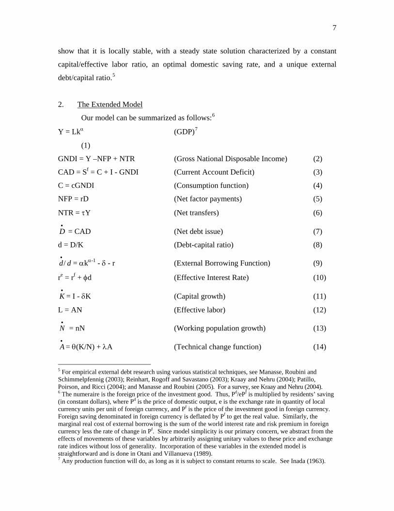
2. The Extended Model

Our model can be summarized as follows:6

Y = Lkα (GDP)7

(1)

GNDI = Y –NFP + NTR (Gross National Disposable Income) (2)

CAD = Sf = C + I - GNDI (Current Account Deficit) (3)

C = cGNDI (Consumption function) (4)

NFP = rD (Net factor payments) (5)

NTR = τY (Net transfers) (6) •

D = CAD (Net debt issue) (7)

d = D/K (Debt-capital ratio) (8)

dd/•

= αkα-1 - δ - r (External Borrowing Function) (9)

re = rf + φd (Effective Interest Rate) (10) •

K = I - δK (Capital growth) (11)

L = AN (Effective labor) (12) •

N = nN (Working population growth) (13) •

A = θ(K/N) + λA (Technical change function) (14)

5 For empirical external debt research using various statistical techniques, see Manasse, Roubini and Schimmelpfennig (2003); Reinhart, Rogoff and Savastano (2003); Kraay and Nehru (2004); Patillo, Poirson, and Ricci (2004); and Manasse and Roubini (2005). For a survey, see Kraay and Nehru (2004). 6 The numeraire is the foreign price of the investment good. Thus, PP

d/ePf is multiplied by residents’ saving (in constant dollars), where Pd is the price of domestic output, e is the exchange rate in quantity of local currency units per unit of foreign currency, and Pf is the price of the investment good in foreign currency. Foreign saving denominated in foreign currency is deflated by Pf to get the real value. Similarly, the marginal real cost of external borrowing is the sum of the world interest rate and risk premium in foreign currency less the rate of change in Pf. Since model simplicity is our primary concern, we abstract from the effects of movements of these variables by arbitrarily assigning unitary values to these price and exchange rate indices without loss of generality. Incorporation of these variables in the extended model is straightforward and is done in Otani and Villanueva (1989). 7 Any production function will do, as long as it is subject to constant returns to scale. See Inada (1963).

8

k = K/L (Capital-effective labor ratio) (15)

Here, Y is real GDP, K is physical capital stock, L is effective labor (in efficiency

units, man-hours or man-days), A is labor-augmenting technology (index number), N is

working population, k is the capital-effective labor ratio, GNDI is gross national

disposable income, NFP is net factor payments, NTR is net transfers, CAD is external

current account deficit, Sf is saving by non-residents, C is aggregate consumption, I is

gross domestic investment, D is net external debt8, d is the net external debt/capital ratio,

r is the marginal real cost of net external borrowing, re is the effective world interest rate,

rf is the risk-free interest rate; τ, δ, φ, n, λ, and α are positive constants, and θ is the

learning coefficient, as in Villanueva (1994). In a closed economy (when D = 0, Sf = 0)

with technical change partly endogenous (θ > 0), the model reduces to the Villanueva

(1994) model; additionally, if technical change is completely exogenous (θ = 0), the

model reduces to the standard neoclassical (Solow-Swan) model.

Consumption in the extended model reflects the openness of the economy—

consumption is gross national disposable income plus foreign saving less aggregate

investment.9 Here, s = 1-c is the propensity to save out of gross national disposable

income. After we solve for the balanced growth path, we choose a particular value of s

that maximizes social welfare (long-run consumption per unit of L). 10

The transfers/grants parameter τ may be allowed to vary positively with the

domestic savings effort s. Donors are likely to step up their aid to countries with strong

adjustment efforts. Finally, donor aid τ earmarked for education, health, and other labor-

productivity enhancing expenditures is expected to boost the learning coefficient θ.

Foreign saving is equivalent to the external current account deficit, which is equal

to the excess of domestic absorption over national income or, equivalently, to net external

8 D is defined as external liabilities minus external assets; as such, it is positive, zero, or negative as external liabilities exceed, equal, or fall short of, external assets. 9 From the national income identity (3). 10 Thus, the saving ratio s =1-c will be chosen endogenously.

9

borrowing (capital plus overall balance in the balance of payments)—noted in equations

(3) and (7).

The derivation of the effective cost, r, of net external debt, D (= Dgross – A) is as

follows: Assume a linear function for the effective interest rate re = rf + φd, where 0 < φ

< 1 (equation 10); the second term is the spread that is increasing in d.11 Net interest

payments on net external debt

= reDgross - rfA,

= (rf + φd)Dgross - rfA

= rf (Dgross – A) + φdDgross

= rf (Dgross – A) + φ(D/K)Dgross

= rfD + φ(D/K)Dgross

Dividing both sides by D,

r = rf + φDgross/K = rf + φ(D+A)/K = rf + φd+ φ(A/Y)k(α-1) r = rf + φ[d + εk(α-1)]. (16)

where Dgross is gross external liabilities, A is gross external assets, D = Dgross – A, and

A/Y = ε. Assume that the gross external assets, A, are a constant (minimum) fraction of

GDP: A = εY.12 In the case of the Philippines, ε = 0.214 at present.

The optimal decision rule for net external borrowing is specified in equation (9)--at

any moment of time, net external borrowing as percent of the total outstanding net stock

of debt is undertaken at a rate equal to the growth rate of the capital stock plus the

difference between the expected marginal product, net of depreciation, and the marginal

real cost of funds, r.13 When this expected yield-cost differential is zero and k is at its

steady state value k*, the growth rate of net external debt equals the steady-state rate of

capital growth (equals output growth, by the constant returns assumption), and the net

11 An increase in d raises the credit risk and, thus, the spread. 12 A rule of thumb is that the variable A represents 3-4 months of imports. 13 Equations (7) and (9) equate net foreign saving with net foreign borrowing, not strictly true. Net foreign saving (sum of capital, financial, and overall accounts in the balance of payments) includes debt (bonds and loans) and non-debt creating flows (equities and foreign direct investment); both flows use up a portion of GDP, with the latter as dividends and profit remittances abroad. Our variables D and r, respectively, should be interpreted broadly to include equities and foreign direct investment, as well as dividends and profit remittances.

10

external debt as ratio to output stabilizes at a constant level.14 However, this constant

debt level may not necessarily be optimal in the sense of being associated with maximum

consumer welfare. For it to be so, it has to be associated with a particular value of the

domestic saving rate that maximizes long-run consumption per effective labor.

3. Reduced Model

By successive substitutions, the extended model reduces to a system of two

differential equations in k and d.15

/k = {s[(1+τ)k•

k α-1 –rd]/(1-d)} + [(αkα-1-δ -r)d/(1-d)] – [δ/(1-d)]-θk- n-λ

= H(k,d) (17) •

d /d = αkα-1-δ-r = J(k,d) (18)

where r is a function of k and d--given by equation (16).

Long-run equilibrium is obtained by setting the reduced system (17) and (18) to

zero, such that k is constant at k* and d is constant at d*.16 It is characterized by

balanced growth: K, L, and D grow at the same rate θk*+n+λ. It also implies the

condition αk*α-1 - δ - r(d*, k*; rf) = 0, which is the optimal rule for external net

borrowing to cease at the margin.17

14 The steady-state current account balance may be positive (deficit), zero (in balance), or negative

(surplus). This follows from the steady-state solution ( /Y)* = g*d*/k*•

D (α-1), where g* is the steady-state growth rate of output, d* is the steady-state debt-capital ratio, and k* is the steady-state capital-effective labor ratio. As mentioned in footnote 8 and defined by equation (8), the variable d* is the ratio of net external debt (external liabilities minus external assets) to the capital stock and can be positive, zero, or negative. More precisely, -1 < d* < 1, depending on whether the accumulated sum of domestic savings is less than, equal to, or greater than the aggregate capital stock (accumulated sum of aggregate investments). 15 It can be seen that in a closed economy, d = τ = 0, equation (18) drops out and, thus, equation (17) is identical to the Villanueva (1994) model (equation 9, p. 7). Further, with θ = 0, equation (17) reduces to the Solow-Swan model. 16 An asterisk denotes steady-state value of any variable. 17 When the yield-cost differential is zero, net external borrowing as percent of the outstanding net stock of debt proceeds at the steady state growth rate of output.

11

The steady-state solutions for k*, d*, and r* are:

{s[(1+τ)k*(α-1) – r*d*]/(1-d*} – δ/(1-d*) - θk* - n - λ = 0 (19)

d* = [(α- φε)k*(α-1) - δ - rf]/φ (20)

r* = rf + φd*+ φεk*(α-1) (16)’

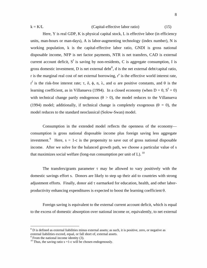
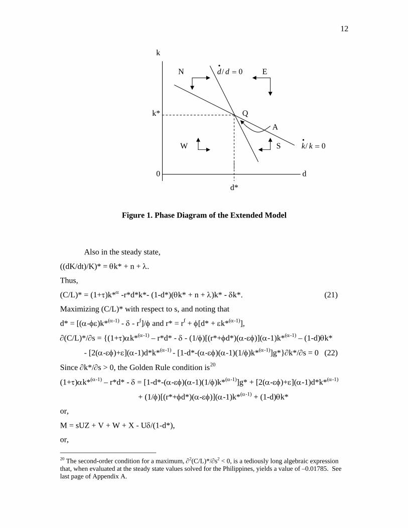
Long-run equilibrium is defined by point Q(d*,k*) in Figure 1.18 In regions N

and W, the dynamics force d to increase, and in regions S and E, the dynamics force d to

decrease. In regions N and E, the dynamics force k to decrease, and, in regions S and W,

the dynamics force k to increase. Any initial point, like point A, leads to a movement

toward the equilibrium point Q, with a possible time path indicated by point A.

In the steady state, output per unit of effective labor is y* = k*α. If y* is

considered a measure of the standard of living, and since dy*/dk* > 0, it is possible to

raise living standards by increasing k*. This can be done by adjusting the domestic

saving rate s, for example, by raising the public sector saving rate and assuming

imperfect Ricardian equivalence.19 If consumption per unit of effective labor is taken as

a measure of the social welfare of the society, the saving rate s that maximizes social

welfare by maximizing long-run consumption can be determined. Phelps (1966) refers to

this path as the “Golden Rule of Accumulation.”

From equation (3), steady-state consumption per unit of effective labor is

(C/L)* = (GNDI/L)* + (Sf/L)* – (I/L)* = (1+τ)k*α - r*d*k* + [((dK/dt)/K)*

+ αk*(α-1) -δ-r*]d*k* - [((dK/dt)/K)* + δ]k*,

and since αk*(α-1) -δ-r* = 0,

= (1+τ)k*α - r*d*k* - (1-d*)k*((dK/dt)/K)* - δk*

where

r* = rf + φ[d* + εk*(α-1)].

18 For the derivation of the slopes of the curves shown in Figure 1, see Appendix A. 19 There is ample empirical evidence that, at least for developing countries, the private sector saving rate does not offset one-to-one the increase in the public sector saving rate.

12

k

N E 0/ =•

dd

k* Q

A

W S 0/ =•

kk

0 d

d*

Figure 1. Phase Diagram of the Extended Model

Also in the steady state,

((dK/dt)/K)* = θk* + n + λ.

Thus,

(C/L)* = (1+τ)k*α -r*d*k*- (1-d*)(θk* + n + λ)k* - δk*. (21)

Maximizing (C/L)* with respect to s, and noting that

d* = [(α-φε)k*(α-1) - δ - rf]/φ and r* = rf + φ[d* + εk*(α-1)],

∂(C/L)*/∂s = {(1+τ)αk*(α-1) – r*d* - δ - (1/φ)[(r*+φd*)(α-εφ)](α-1)k*(α-1) – (1-d)θk*

- [2(α-εφ)+ε](α-1)d*k*(α-1) - [1-d*-(α-εφ)(α-1)(1/φ)k*(α-1)]g*}∂k*/∂s = 0 (22)

Since ∂k*/∂s > 0, the Golden Rule condition is20

(1+τ)αk*(α-1) – r*d* - δ = [1-d*-(α-εφ)(α-1)(1/φ)k*(α-1)]g* + [2(α-εφ)+ε](α-1)d*k*(α-1)

+ (1/φ)[(r*+φd*)(α-εφ)](α-1)k*(α-1) + (1-d)θk*

or,

M = sUZ + V + W + X - Uδ/(1-d*),

or, 20 The second-order condition for a maximum, ∂2(C/L)*/∂s2 < 0, is a tediously long algebraic expression that, when evaluated at the steady state values solved for the Philippines, yields a value of –0.01785. See last page of Appendix A.

13

s = [M – V – W –X + Uδ/(1-d*)]/UZ.21 (23)

where,

M = (1+τ)αk*(α-1) – r*d* - δ;

U = [1-d*-(α-εφ)(α-1)(1/φ)k*(α-1)];

V = [2(α-εφ)+ε] (α-1)d*k*(α-1);

W = (1/φ)[(r*+φd*)(α-εφ)](α-1)k*(α-1);

X = (1-d*)θk*; and

Z = [(1+τ)k*(α-1) – r*d*]/(1-d*).

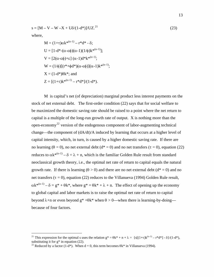
M is capital’s net (of depreciation) marginal product less interest payments on the

stock of net external debt. The first-order condition (22) says that for social welfare to

be maximized the domestic saving rate should be raised to a point where the net return to

capital is a multiple of the long-run growth rate of output. X is nothing more than the

open-economy22 version of the endogenous component of labor-augmenting technical

change—the component of (dA/dt)/A induced by learning that occurs at a higher level of

capital intensity, which, in turn, is caused by a higher domestic saving rate. If there are

no learning (θ = 0), no net external debt (d* = 0) and no net transfers (τ = 0), equation (22)

reduces to αk*(α-1) – δ = λ + n, which is the familiar Golden Rule result from standard

neoclassical growth theory, i.e., the optimal net rate of return to capital equals the natural

growth rate. If there is learning (θ > 0) and there are no net external debt (d* = 0) and no

net transfers (τ = 0), equation (22) reduces to the Villanueva (1994) Golden Rule result,

αk*(α-1) – δ = g* + θk*, where g* = θk* + λ + n. The effect of opening up the economy

to global capital and labor markets is to raise the optimal net rate of return to capital

beyond λ+n or even beyond g* +θk* when θ > 0—when there is learning-by-doing—

because of four factors.

21 This expression for the optimal s uses the relation g* = θk* + n + λ = {s[(1+τ)k(α-1) – r*d*] - δ}/(1-d*), substituting it for g* in equation (22). 22 Reduced by a factor (1-d*). When d = 0, this term becomes θk* in Villanueva (1994).

14

First, when the domestic saving rate s is raised, the equilibrium growth rate g*

will be higher than λ+n, by the amount of θ∂k*/∂s. Second, capital should be

compensated for the effect on equilibrium output growth through the induced learning

term θk*. Third, when the domestic saving rate is raised, the equilibrium debt stock d*

will be lower, releasing resources toward more capital growth; the effective interest rate

r* also will be lower pari passu with a lower spread, further increasing domestic

resources for investment and growth. Fourth, the availability of foreign saving to finance

capital accumulation enhances long-run growth, up to a point.

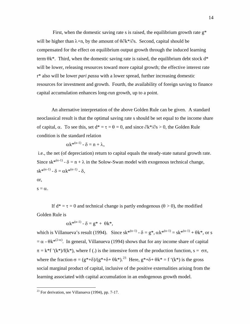
An alternative interpretation of the above Golden Rule can be given. A standard

neoclassical result is that the optimal saving rate s should be set equal to the income share

of capital, α. To see this, set d* = τ = θ = 0, and since ∂k*/∂s > 0, the Golden Rule

condition is the standard relation

αk*(α-1) - δ = n + λ,

i.e., the net (of depreciation) return to capital equals the steady-state natural growth rate.

Since sk*(α-1) - δ = n + λ in the Solow-Swan model with exogenous technical change,

sk*(α-1) - δ = αk*(α-1) - δ,

or,

s = α.

If d* = τ = 0 and technical change is partly endogenous (θ > 0), the modified

Golden Rule is

αk*(α-1) - δ = g* + θk*,

which is Villanueva’s result (1994). Since sk*(α-1) - δ = g*, αk*(α-1) = sk*(α-1) + θk*, or s

= α - θk*(2-α). In general, Villanueva (1994) shows that for any income share of capital

π = k*f ’(k*)/f(k*), where f (.) is the intensive form of the production function, s = σπ,

where the fraction σ = (g*+δ)/(g*+δ+ θk*).23 Here, g*+δ+ θk* = f ‘(k*) is the gross

social marginal product of capital, inclusive of the positive externalities arising from the

learning associated with capital accumulation in an endogenous growth model.

23 For derivation, see Villanueva (1994), pp. 7-17.

15

Equivalently put, income going to capital as a share of total output should be a multiple

of the amount saved and invested in order to compensate capital for the additional output

generated by endogenous growth and induced learning. A value of π equal to s, implicit

in the standard model, would undercompensate capital and thus be suboptimal from a

societal point of view.

The open economy’s optimal domestic saving rate, given by equation (23), is

higher than α - θk*(2-α) given by Villanueva (1994), reflecting the inherent risks involved

in foreign borrowing.24

In general, the existence, uniqueness, and stability of the steady state equilibrium

are not guaranteed. However, Appendix A shows that for a Cobb-Douglas production

function, linear ‘learning-by-doing’ and risk-premium functions, and values of the

parameters for the Philippines, the extended model’s equilibrium is locally stable in the

neighborhood of the steady state.25

III. Application to the Philippines

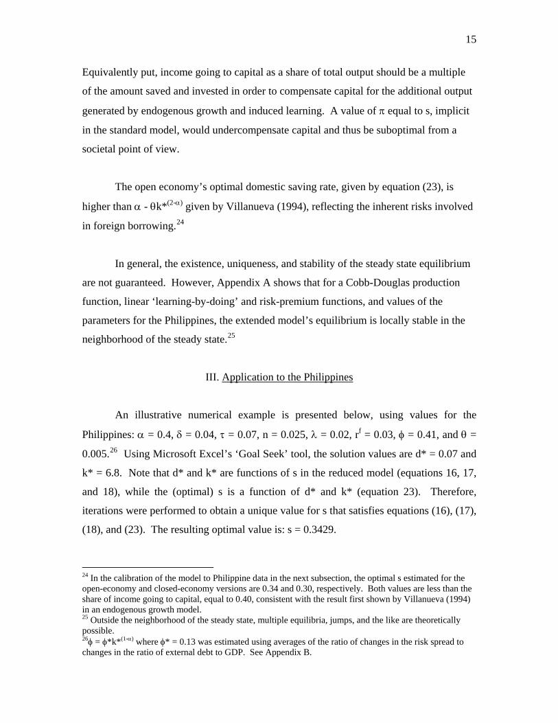
An illustrative numerical example is presented below, using values for the

Philippines: α = 0.4, δ = 0.04, τ = 0.07, n = 0.025, λ = 0.02, rf = 0.03, φ = 0.41, and θ =

0.005.26 Using Microsoft Excel’s ‘Goal Seek’ tool, the solution values are d* = 0.07 and

k* = 6.8. Note that d* and k* are functions of s in the reduced model (equations 16, 17,

and 18), while the (optimal) s is a function of d* and k* (equation 23). Therefore,

iterations were performed to obtain a unique value for s that satisfies equations (16), (17),

(18), and (23). The resulting optimal value is: s = 0.3429.

24 In the calibration of the model to Philippine data in the next subsection, the optimal s estimated for the open-economy and closed-economy versions are 0.34 and 0.30, respectively. Both values are less than the share of income going to capital, equal to 0.40, consistent with the result first shown by Villanueva (1994) in an endogenous growth model. 25 Outside the neighborhood of the steady state, multiple equilibria, jumps, and the like are theoretically possible. 26φ = φ*k*(1-α) where φ* = 0.13 was estimated using averages of the ratio of changes in the risk spread to changes in the ratio of external debt to GDP. See Appendix B.

16

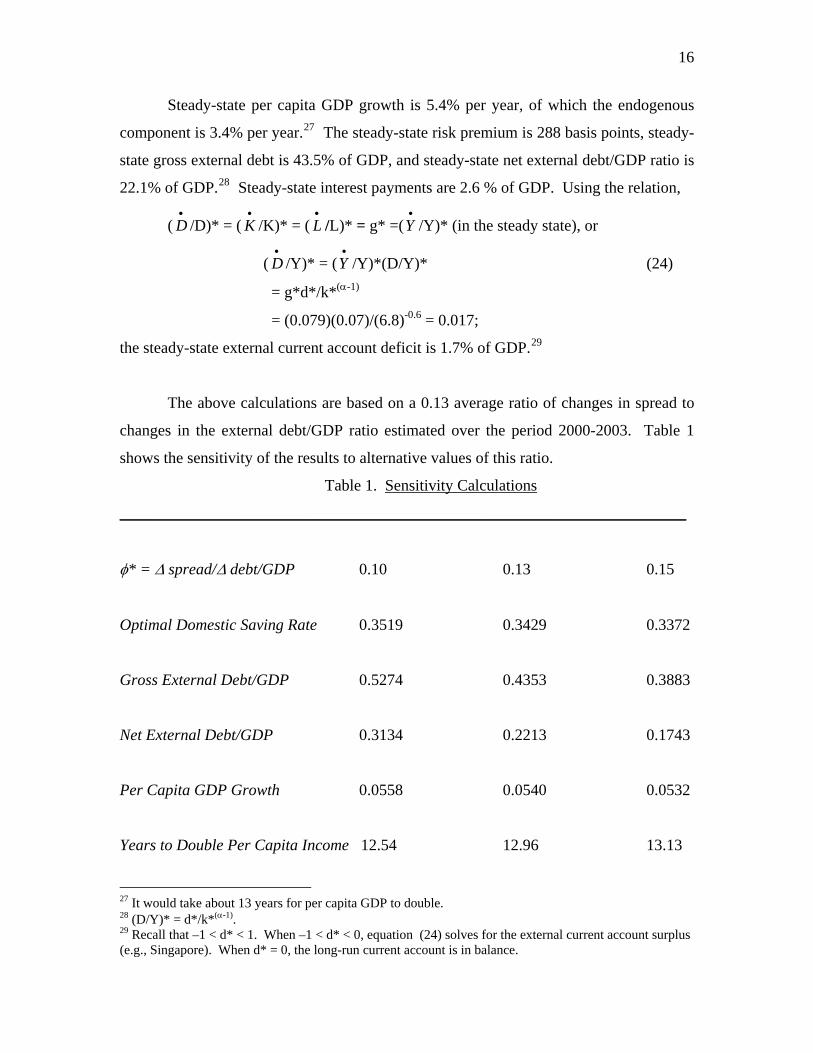
Steady-state per capita GDP growth is 5.4% per year, of which the endogenous

component is 3.4% per year.27 The steady-state risk premium is 288 basis points, steady-

state gross external debt is 43.5% of GDP, and steady-state net external debt/GDP ratio is

22.1% of GDP.28 Steady-state interest payments are 2.6 % of GDP. Using the relation,

( /D)* = (•

D•

K /K)* = ( /L)* = g* =(•

L•

Y /Y)* (in the steady state), or

( /Y)* = (•

D•

Y /Y)*(D/Y)* (24)

= g*d*/k*(α-1)

= (0.079)(0.07)/(6.8)-0.6 = 0.017;

the steady-state external current account deficit is 1.7% of GDP.29

The above calculations are based on a 0.13 average ratio of changes in spread to

changes in the external debt/GDP ratio estimated over the period 2000-2003. Table 1

shows the sensitivity of the results to alternative values of this ratio.

Table 1. Sensitivity Calculations

_______________________________________________________________________

φ* = Δ spread/Δ debt/GDP 0.10 0.13 0.15

Optimal Domestic Saving Rate 0.3519 0.3429 0.3372

Gross External Debt/GDP 0.5274 0.4353 0.3883

Net External Debt/GDP 0.3134 0.2213 0.1743

Per Capita GDP Growth 0.0558 0.0540 0.0532

Years to Double Per Capita Income 12.54 12.96 13.13

27 It would take about 13 years for per capita GDP to double. 28 (D/Y)* = d*/k*(α-1). 29 Recall that –1 < d* < 1. When –1 < d* < 0, equation (24) solves for the external current account surplus (e.g., Singapore). When d* = 0, the long-run current account is in balance.

17

The estimated optimal domestic saving rate, steady-state per capita GDP growth

rate, and the number of years it would take for per capita GDP to double are robust to

alternative values of the ratio of changes in spread to changes in the external debt/GDP

ratio of 0.10 to 0.15. However, as expected, the steady state gross external debt/GDP

ratio declines from 53% to 39%, and the steady state net external debt/GDP ratio from

31% to 17%, as the sensitivity of the spread to the debt ratio rises from 0.10 to 0.15.

In the Philippines, optimal long-run growth requires raising the domestic saving

rate from the historical average of 18.8% of GNP30 during 1993-98 to a steady state 34%

over the long term. This is necessary to achieve external viability while maximizing

long-run consumption per effective labor. The savings effort should center on fiscal

consolidation and adoption of incentives to encourage private saving, including market-

determined real interest rates. From the national income identity (3), the external current

account deficit CAD is equal to the excess of aggregate investment I over domestic

saving S (= GNDI – C), or CAD = I – S. Decomposing I and S into their government and

private components, CAD = (Ig – Sg) + (Ip – Sp), where the subscripts g and p denote

government and private, respectively. The first term is the fiscal balance, and the second

term is the private sector balance. Fiscal adjustment is measured in terms of policy

changes in Sg (government revenue less consumption) and in Ig (government investment).

Given estimates of the private sector saving-investment balance and its components, the

optimal government saving-investment balance may be derived as a residual; from this,

the required government saving ratio can be calculated because the optimal growth model

implies a government investment ratio.

Assume, however, the following hypothetical worst case-scenario for the

Philippines. For whatever reason (political, social, etc.), owing to the initial high level of

the external debt, market perceptions reach a very high adverse level. Despite a high-

expected marginal product of capital, the risk premium is prohibitively high at any level

of the debt ratio and the risk-free interest rate, such that the Philippine public sector faces

30 Source: Philippine Statistical Appendix, IMF Staff Country Report 99/93 (International Monetary Fund, August 1999), Table 5.

18

credit rationing. 31 In such circumstances, as Agénor (op. cit., p. 595-96) suggests,

increased foreign aid targeted at investment broadly defined to include physical and

human capital may benefit the Philippines, provided that economic policies are sound.

IV. Implications for Fiscal Policy and External Debt Management

The implications for fiscal policy and external debt management are clear for the

Philippines. The first step is to launch an effective external debt management strategy

that will articulate the short and long run objectives of fiscal policy and debt management

and ensure effective centralized approval and monitoring of primary debt issues to global

financial markets, aided by (i) detailed electronic data on external debt, both outstanding

and new debt, by borrowing institution, maturity, terms, etc., and by (ii) an inter-agency

desk exclusively responsible for top quantitative and analytic work on external debt for

the benefit of policy-makers.

The level of external debt can be reduced only by cutting the fiscal deficit

immediately and at a sustained pace over the medium term. In this context, the

privatization of the National Power Corporation (NAPOCOR) is essential, since a big

chunk of sovereign debt issues is on behalf of NAPOCOR.

Interest payments on total government debt currently eat up a significant share of

government revenues, leaving revenue shortfalls to cover expenditures on the physical

infrastructure and on the social sectors (health, education, and the like). With a

successful and steady reduction of the stock of debt and the enhancement of domestic

savings led by the government sector (via increases in Sg), the sensitivity of the risk

spread to the external debt would decrease, resulting in interest savings that would

provide additional financing for the infrastructure and social sectors. Furthermore, there

are clear implications for both revenue-raising and expenditure-cutting measures. On the

revenue side, although the recently enacted and signed VAT bill is welcome, there

31 The credit risk is included in the risk premium. The higher is the credit risk assigned by international creditors/investors, the higher is the risk premium and consequently, the higher is the effective real interest rate.

19

remains low compliance on the VAT, resulting in very low collections. There is evidence

of VAT sales being substantially under-declared on a regular basis. Our concrete

proposal would be to set up a computerized system of VAT sales wherein an electronic

copy of the sales receipt is transmitted in real time by merchants, producers, and service

providers to the Bureau of Internal Revenue (BIR). In this manner total sales subject to

the VAT submitted come tax time can be compared by the BIR against its own electronic

receipts. It is estimated that if only 50% of total sales were collected from VAT, the

current budget deficit (some P200+ billion) could be wiped out. This proposal easily

beats current proposals to raise taxes because as they stand, marginal tax rates are already

very high (resulting in tax evasion and briberies). The imposition of “sin” taxes (on

cigarettes and liquor sales) would provide little relief. Individual and corporate tax

reforms are also necessary--different tax brackets should be consolidated into a few, with

significant reductions in marginal income tax rates; at the same time, the number of

exemptions should be drastically reduced to widen the tax base. The whole customs

tariffs structure should be reviewed with the aim of reducing average tariff rates further,

while eliminating many exemptions. The role of the customs assessor and collector

should be severely restricted, with computerized assessment and collection being put in

place, similar to our VAT proposal.

V. Conclusion

This paper has explored the joint dynamics of external debt, capital accumulation,

and growth. The relative simplicity of our model makes it convenient to analyze the links

between domestic adjustment policies, foreign borrowing, and growth. We estimate the

optimal domestic saving rate for the Philippines that is consistent with maximum real

consumption per unit of effective labor in the long run. As a by-product, we estimate the

steady-state ratio of net external debt to GDP that is associated with this optimal

outcome. The framework is an extension of the standard neoclassical growth model that

incorporates endogenous technical change and global capital markets. The major policy

implications are that in the long run, fiscal adjustment and the promotion of private

saving are critical; reliance on foreign saving in a globalized financial world has limits,

20

and when risk spreads are highly and positively correlated with rising external debt

levels, unabated foreign borrowing depresses long run welfare.

The obvious policy conclusions of the extended model are:

1. Fiscal consolidation and strong incentives for private saving are essential

to achieving maximum per capita GDP growth;

2. The domestic saving rate should be set below the share of capital in total

output, owing to positive externalities arising from learning-by-doing

associated with capital accumulation. Equivalently put, income going to

capital as a share of total output should be a multiple of the amount saved

and invested in order to compensate capital for the additional output

generated by endogenous growth and induced learning.

3. Reliance on foreign savings (external borrowing) has limits, particularly in

a global environment of high interest rates and risk spreads;

4. When real borrowing costs are positively correlated with rising external

indebtedness, the use of foreign savings is even more circumscribed;

5. When risk spreads are prohibitively high despite high-expected marginal

product of capital, there is a role for increased foreign aid earmarked for

education and health, provided that economic policies are sound.

21

Appendix A: Stability Analysis

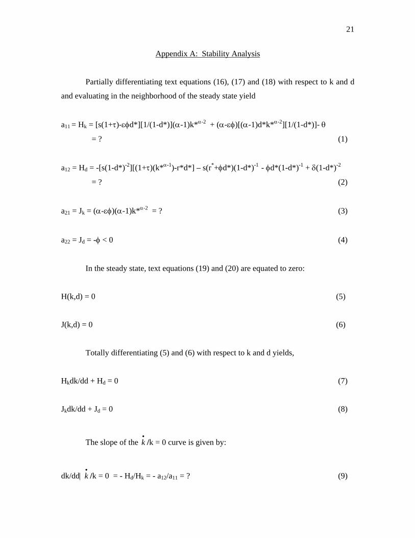
Partially differentiating text equations (16), (17) and (18) with respect to k and d

and evaluating in the neighborhood of the steady state yield

a11 = Hk = [s(1+τ)-εφd*][1/(1-d*)](α-1)k*α-2 + (α-εφ)[(α-1)d*k*α-2][1/(1-d*)]- θ

= ? (1)

a12 = Hd = -[s(1-d*)-2][(1+τ)(k*α-1)-r*d*] – s(r*+φd*)(1-d*)-1 - φd*(1-d*)-1 + δ(1-d*)-2

= ? (2)

a21 = Jk = (α-εφ)(α-1)k*α-2 = ? (3)

a22 = Jd = -φ < 0 (4)

In the steady state, text equations (19) and (20) are equated to zero:

H(k,d) = 0 (5)

J(k,d) = 0 (6)

Totally differentiating (5) and (6) with respect to k and d yields,

Hkdk/dd + Hd = 0 (7)

Jkdk/dd + Jd = 0 (8)

The slope of the /k = 0 curve is given by: •

k

dk/dd| /k = 0 = - H•

k d/Hk = - a12/a11 = ? (9)

22

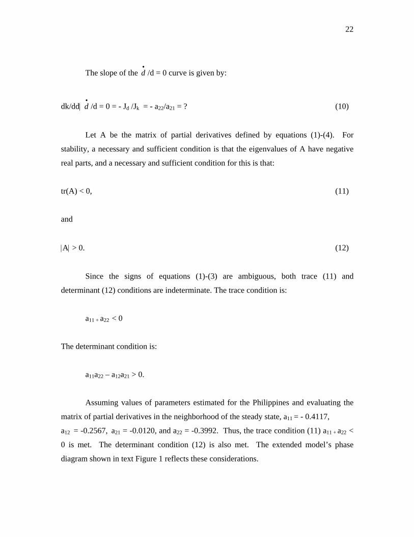
The slope of the /d = 0 curve is given by: •

d

dk/dd| /d = 0 = - J•

d d /Jk = - a22/a21 = ? (10)

Let A be the matrix of partial derivatives defined by equations (1)-(4). For

stability, a necessary and sufficient condition is that the eigenvalues of A have negative

real parts, and a necessary and sufficient condition for this is that:

tr(A) < 0, (11)

and

|A| > 0. (12)

Since the signs of equations (1)-(3) are ambiguous, both trace (11) and

determinant (12) conditions are indeterminate. The trace condition is:

a11 + a22 < 0

The determinant condition is:

a11a22 – a12a21 > 0.

Assuming values of parameters estimated for the Philippines and evaluating the

matrix of partial derivatives in the neighborhood of the steady state, a11 = - 0.4117,

a12 = -0.2567, a21 = -0.0120, and a22 = -0.3992. Thus, the trace condition (11) a11 + a22 <

0 is met. The determinant condition (12) is also met. The extended model’s phase

diagram shown in text Figure 1 reflects these considerations.

23

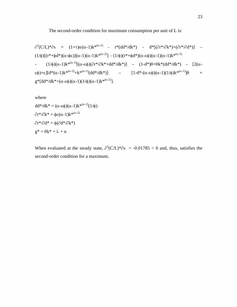
The second-order condition for maximum consumption per unit of L is:

∂2(C/L)*∂s = (1+τ)α(α-1)k*(α-2) - r*(dd*/dk*) - d*[(∂r*/∂k*)+(∂r*/∂d*)] –

(1/φ)[(r*+φd*)(α-φε)](α-1)(α-1)k*(α-2)] – (1/φ)(r*+φd*)(α-εφ)(α-1)(α-1)k*(α-2)

- (1/φ)(α-1)k*(α-1)[(α-εφ)(∂r*/∂k*+dd*/dk*)] – (1-d*)θ+θk*(dd*/dk*) - [2(α-

εφ)+ε][d*(α-1)k*(α-2)+k*(α-1)(dd*/dk*)] – [1-d*-(α-εφ)(α-1)(1/φ)k*(α-1)]θ +

g*[dd*/dk*+(α-εφ)(α-1)(1/φ)(α-1)k*(α-2)].

where

dd*/dk* = (α-εφ)(α-1)k*(α-2)(1/φ)

∂r*/∂k* = φε(α-1)k*(α-2)

∂r*/∂d* = φ(∂d*/∂k*)

g* = θk* + λ + n

When evaluated at the steady state, ∂2(C/L)*∂s = -0.01785 < 0 and, thus, satisfies the

second-order condition for a maximum.

24

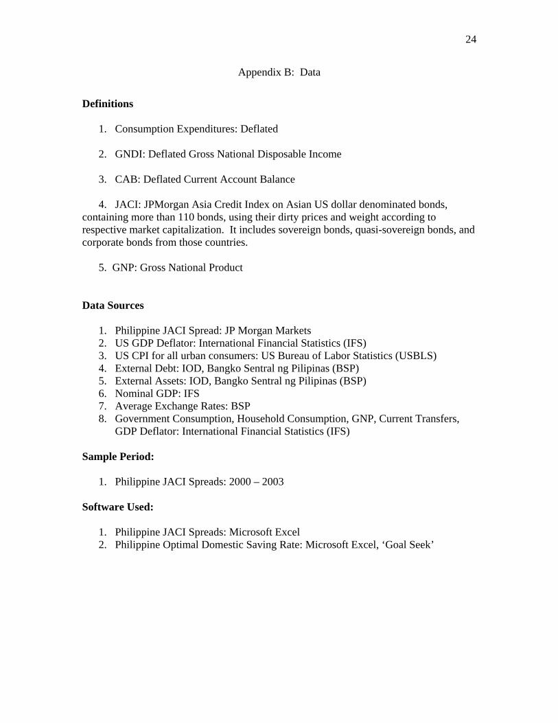
Appendix B: Data

Definitions

1. Consumption Expenditures: Deflated 2. GNDI: Deflated Gross National Disposable Income

3. CAB: Deflated Current Account Balance

4. JACI: JPMorgan Asia Credit Index on Asian US dollar denominated bonds,

containing more than 110 bonds, using their dirty prices and weight according to respective market capitalization. It includes sovereign bonds, quasi-sovereign bonds, and corporate bonds from those countries.

5. GNP: Gross National Product Data Sources

1. Philippine JACI Spread: JP Morgan Markets 2. US GDP Deflator: International Financial Statistics (IFS) 3. US CPI for all urban consumers: US Bureau of Labor Statistics (USBLS) 4. External Debt: IOD, Bangko Sentral ng Pilipinas (BSP) 5. External Assets: IOD, Bangko Sentral ng Pilipinas (BSP) 6. Nominal GDP: IFS 7. Average Exchange Rates: BSP 8. Government Consumption, Household Consumption, GNP, Current Transfers,

GDP Deflator: International Financial Statistics (IFS) Sample Period:

1. Philippine JACI Spreads: 2000 – 2003 Software Used:

1. Philippine JACI Spreads: Microsoft Excel 2. Philippine Optimal Domestic Saving Rate: Microsoft Excel, ‘Goal Seek’

25

References

1. Agénor, Pierre-Richard (2000), The Economics of Adjustment and Growth,

San Diego, Academic Press, 591-96.

2. Arrow, Kenneth (1962), “The Economic Implications of Learning-by-Doing,”

Review of Economic Studies, 29, 155-73.

3. Becker, Gary, Kevin Murphy, and Robert Tamura (1990), “Human Capital,

Fertility, and Economic Growth,” Journal of Political Economy, 98, S12-37.

4. Conlisk, John (1967), “A Modified Neo-Classical Growth Model with

Endogenous Technical Change,” The Southern Economic Journal, 34, 199-208. 5. Grossman, Gene and Elhanan Helpman (1990), “Comparative Advantage and

Long-Run Growth,” American Economic Review, 80, 796-815.

6. Inada, Ken-ichi (1963), “On a Two-Sector Model of Economic Growth:

Comments and Generalization,” Review of Economic Studies, 30, 119-27.

7. Kraay, Aart and Vikram Nehru (2004), “When Is External Debt Sustainable?”

World Bank Policy Research Working Paper 3200, February.

8. Lucas, Robert (1988), “On the Mechanics of Economic Development,” Journal of

Monetary Economics, 22, 3-42.

9. Manasse, Paolo and Nouriel Roubini (2005), “Rules of Thumb for Sovereign

Debt Crises,” WP/05/42, International Monetary Fund.

10. Manasse, Paolo, Nouriel Roubini, and Axel Schimmelpfenning (2003),

“Predicting Sovereign Debt Crises,” Manuscript, University of Bologna, IMF

and New York University.

11. Otani, Ichiro and Delano Villanueva, “Theoretical Aspects of Growth in

Developing Countries: External Debt Dynamics and the Role of Human Capital,”

IMF Staff Papers, 36, 307-42.

12. Patillo, Catherine, Helene Poirson, and Luca Ricci (2004), “What Are The

Channels Through Which External Debt Affects Growth,” IMF WP/04/15,

January.

13. Phelps, Edmund (1966), Golden Rules of Economic Growth, New York, W.W.

26

Norton.

14. Reinhart, Carmen, Kenneth Rogoff, and Miguel Savastano (2003), “Debt

Intolerance,” Brookings Papers on Economic Activity, forthcoming.

15. Rivera-Batiz, Luis and Paul Romer (1991), “International Trade with

EndogenousTechnical Change,” NBER Working Paper 3594, Washington,

National Bureau of Economic Research.

16. Romer, Paul (1986), “Increasing Returns and Long-Run Growth,” Journal of

Political Economy, 94, 1002-37.

17. Roubini, Nouriel (2001), “Debt Sustainability: How to Assess Whether a Country

Is Insolvent,” Stern School of Business, New York University, December 20.

18. Solow, Robert (1956), “A Contribution to the Theory of Economic Growth,”

The Quarterly Journal of Economics, 70, 65-94.

19. Swan, Trevor (1956), “Economic Growth and Capital Accumulation,”

Economic Record, 32, 334-62.

20. Villanueva, Delano (1994), “Openness, Human Development, and Fiscal

Policies: Effects on Economic Growth and Speed of Adjustment,”

IMF Staff Papers, 41, 1-29.

21. ________________(2003), “External Debt, Capital Accumulation and Growth,” SMU-SESS Discussion Paper Series in Economics and Statistics.