Export Intensity and Input Trade Liberalization: Evidence ... · We thank Andrew Bernard, Robert Feenstra, Gordon Hanson, Samuel Kortum, Zhiyuan Li, Justin Lin, Robert Staiger, James

Export Intensity and Input Trade Liberalization: Evidence fromChinese Firms�

Miaojie Yuy Wei Tianz

China Center for Economic Research Guanghua School of ManagementPeking University Peking University

February 26, 2013

Abstract

How do reductions in input trade costs a¤ect �rms�sales decision between domestic and foreign

markets? By using Chinese �rm-level production data and transaction-level trade data during 2000-

2006 to construct �rm-speci�c input trade costs, We �nd rich evidence that a reduction in input

trade cost for large trading �rms leads to an increase in export intensity (exports over total sales).

We argue both theoretically and empirically that such a �nding occurs via both the extensive margin

and the intensive margin. A fall in input tari¤s serves as a cost-saving e¤ect to induce more non-

exporting �rms to export (the extensive margin). More importantly, a reduction in input tari¤s also

causes existing exporters to increase their export intensity (the intensive margin) since, compared

with domestic sectors, exporting sectors use more and better imported intermediate inputs. The

results are robust to di¤erent empirical speci�cations and econometric methods.

JEL: F1, F2

Keywords: Export Intensity, Input Trade Costs, Imported Intermediate Inputs, Processing

Trade

�We thank Andrew Bernard, Robert Feenstra, Gordon Hanson, Samuel Kortum, Zhiyuan Li, Justin Lin, RobertStaiger, James Tybout, Yang Yao, and seminar and conference participants from the 14th NBER-CCER conference, the2nd China Trade Research Group (CTRG) conference, the 3rd IEFS (China) conference, BREAD-Guanghua summerschool, Zhejiang University, Nankai University, and Shanghai School of Foreign Trade for their helpful comments andconstructive suggestions. However, all errors are ours.

yChina Center for Economic Research (CCER), National School of Development, Peking University, Beijing 100871,China. Phone: 86-10-6275-3109, Fax: 86-10-6275-1474, E-mail: [email protected].

zDepartment of Applied Economics, Guanghua School of Management, Peking University. Email:[email protected].

1 Introduction

Firms�self-selection to engage in domestic and/or foreign markets is one of the most tropical topics

a hot topic in international trade. It is of particular interest for both academia and policy makers

to understand the �rm�s decision in choosing markets when a country experiences gradual trade lib-

eralization. Traditionally, import tari¤ reductions on �nal goods have been regarded as generating

tougher import competition, which in turn forces domestic �rms to adjust their export intensity�the

proportion of exports over total sales. Today, research interest in trade liberalization has switched from

output tari¤ reductions to input tari¤ reductions (see, for example, Amiti and Konings 2007; Topalova

and Khandelwal 2011). Yet, there is still relatively little research on �rms�response in adjusting their

export intensity upon facing input tari¤ reductions. The present paper tries to �ll this gap.

The paper investigates the impact of input tari¤ reductions on export intensity for Chinese large

trading �rms. It uses a rich, matched, Chinese �rm-level production and transaction-level trade data

set over the sample period 2000-2006. A novel element of the paper is that input trade costs are

measured at and tailored to the �rm level, which allows us to exactly measure the input trade costs

faced by a �rm, and accordingly to explore the variation of input trade costs within an industry.

To accurately estimate the impact of input trade costs on export intensity, we control for two other

types of trade liberalization: import tari¤s on �nal goods and external tari¤s set by Chinese trading

partners. Output tari¤ reduction in �nal goods generates tougher import competition, which could

in turn change �rms�export intensity. During 2000-2006, many Chinese �rms exported a variety of

products to many countries. Chinese exporters also enjoyed large tari¤ reductions in their export

destinations. With reductions in foreign trade costs, �rms are able to access larger foreign markets,

which could possibly result in greater export intensity. We hence construct �rm-level external tari¤s to

measure weighted tari¤s across trading countries and across products over time. The most ideal way

to do this would be to obtain the corresponding �rm-level import and output tari¤s; however, domestic

sales data for each product are unavailable. Therefore, we only control for industry-level output and

import tari¤s in the estimates. Our estimates suggest that, overall, input tari¤ reduction leads to an

1

increase in export intensity.

China�s processing trade provides an ideal quasi-natural experiment platform to examine the impact

of input tari¤ reduction on export intensity. As perhaps the most important feature of international

trade in China, processing trade refers to the process by which a domestic �rm initially obtains raw

materials or intermediate inputs abroad, and, after local processing, exports value-added �nal goods.

Processing trade in China enjoys the privilege of tari¤ exemptions. Thus, input tari¤ reductions should

not have any impact on �rms�processing exports given that processing imports are already duty-free

by de�nition. We hence decompose �rms�total exports into processing exports and ordinary exports.

As anticipated, input tari¤ reduction does not have any signi�cant impact on �rms�processing exports,

whereas it has a statistically signi�cant impact on �rms�ordinary exports.

We then seek to understand the channels and mechanisms for such a �nding. Declining input

trade costs induce �rms to access more imported intermediate inputs, which in turn transfer to higher

export intensity through both the extensive margin and the intensive margin. On the one hand, a

further reduction in input tari¤s leads to an increase in �rms� total pro�t. Thus, �rms that were

not able to enter the foreign market now self-select to export since they can cover the �xed costs of

exporting (Melitz 2003). That is, the reduction in �rm input tari¤s a¤ects �rms� export intensity

(i.e., the extensive margin). On the other hand, the reduction in �rm input tari¤s also a¤ects �rms�

export intensity through the intensive margin by increasing the proportion of foreign sales for existing

exporters, which occurs through two mechanisms.

Consider a �rm that has two plants: one produces goods for domestic sales whereas the other

produces for foreign sales. First, if the imported intermediate inputs ratio, de�ned as imported inter-

mediate inputs divided by total intermediate inputs, for producing export goods is higher than that for

producing domestic goods, declining input tari¤s could generate higher export intensity since export-

ing sectors bene�t more from input tari¤ reduction. Second, as documented by other studies, such as

Helpern et al. ( 2010) and con�rmed by using Chinese data, imported intermediate inputs are usually

of better quality than domestic intermediate inputs due to more stringent international regulations on

product quality (Levchenko 2007). The increase in imported intermediate inputs caused by input trade

liberalization leads to higher-quality �nal products. Holding other factors constant, exporting �rms

2

could produce more competitive and favorable products for international markets and hence export

more. To elaborate this, we deliver a simple Melitz-type model to enrich our understanding of this

mechanism.

An intensive empirical search provides ample evidence to support our theoretical propositions.

The impact of input trade liberalization on export intensity is shown to be more pronounced for

those �rms with more imported varieties. By adopting a Tobit type-2 selection model, we see that

declining input tari¤s lead to a higher probability for �rms to export. If �rms export, they have

greater export intensity with declining input trade costs. That is, we �nd strong evidence for both

the extensive margin and the intensive margin. We also �nd rich evidence that exporting �rms have

a higher imported intermediate inputs ratio: exporters use more imported intermediate inputs than

non-exporters, even controlling for various �rm characteristics�such as total factor productivity (TFP),

size, and sales�by adopting the nearest-neighbor matching approach. A similar �nding applies to pure

exporters (i.e., all products are sold abroad) versus non-pure exporters. Meanwhile, we see that the

unit-value, a proxy for product quality, of intermediate inputs for processing imports is higher than

its counterpart for ordinary imports. This �nding provides further evidence to support our theoretical

conjecture that imported intermediate inputs are usually of better quality than domestic intermediate

inputs.

The endogeneity of �rm input tari¤s is also carefully discussed and addressed. A well-known

endogeneity is of the measured �rm-weighted input tari¤s. Using �rms�contemporary imports for each

product to construct its weight may raise the issue of endogeneity. Suppose a �rm faces a prohibitive

tari¤ line for a product that it wishes to import; such a tari¤ is not included in the �rm�s input tari¤s

due to its zero imports. However, the �rm indeed faces a high (not zero) tari¤. To control for these

two endogeneity issues, throughout the paper we use �rms�imports in the �rst year of the sample to

construct a �xed weight for �rm-speci�c input tari¤s following Topalova and Khandelwal (2011).

There also exist two other types of endogeneity caused by possible reverse causality. First, as �rms�

export intensity is de�ned as exports over sales; �rms�sales may have reverse causality on tari¤s. Firms

with a small amount of sales may blame their tough market situation on stronger import competition

due to trade liberalization. Accordingly, they would lobby the government for protection. Second,

3

�rms�exports may reversely a¤ect tari¤ formation since �rms�exports are highly correlated with their

imports (Feng et al. 2012). We therefore adopt an instrumental variable (IV) approach to control for

endogeneity. Our IV estimates still suggest that input tari¤ reduction leads to an increase in export

intensity.

Finally, we perform two important robustness checks. The �rst exercise considers the relative im-

portance of domestic intermediate inputs against imported intermediate inputs. We use this di¤erence

to construct an alternative measure of input tari¤s, which also suggests very similar results as our

previous estimates: declining trade costs lead to an increase in export intensity. Our second robust-

ness check is to adopt quantile estimates to examine the heterogeneous impact of input trade costs on

�rms�export intensity at di¤erent quantiles. We �rst look at the response of each of the four quartiles,

and then examine the quantile estimates in a continuous version. Both types of quantile analysis yield

similar results as the standard �xed-e¤ects ordinary least squares (OLS) estimates. They also help us

understand the economic magnitude of the estimates: a one standard deviation reduction in a �rm�s

input tari¤ would lead to around a 0.9 to 2.8 percent increase in its export intensity.

The present paper joins a growing literature on the topic of export intensity. Previous studies have

recognized that �rms only sell a small fraction of their output abroad. This is documented by, among

others, Bernard and Jensen (1995), Tybout (2000) , Bernard et al. (2010), Arkolakis and Muendler

(2010), and Eaton et al. (2011). Most of such studies focus on interpreting why export intensity is

small. Speci�cally, Bernard et al. (2003) emphasize that a key reason for large countries like the

United States is the existence of a relatively large domestic market. Brooks (2006) argues that the

key reason for small countries like Colombia is the low quality of their export products. Bonaccorsi

(1992) �nds evidence that �rms�export intensity is positively associated with their size, using Italian

manufacturing industry-level data. Greenaway et al. (2004) investigate whether spillovers a¤ect �rms�

export propensity, using British �rm-level data.

However, there has been limited research on China, although it has become the second largest

economy and the largest exporter in the world. As documented later, although China shares a common

phenomenon with other countries in the sense that Chinese �rms only export a small proportion of

their products, a sizable proportion of Chinese �rms exports all of their products. Such a pattern is

4

known as a U-shape, as described by Lu (2011).1 Therefore, it is worthwhile to ask how declining input

trade costs a¤ect such Chinese �rms�export pattern, which hence adds value to the related literature.

A related branch of the literature is on input trade liberalization. Among many other papers,

Amiti and Konings (2007), using Indonesian �rm-level data, �nd that �rms gain from the reduction

of input tari¤s at least twice as much as from cutting output tari¤s. Topalova and Khandelwal (2011)

con�rm that such a di¤erence in gains from trade could be exaggerated to approximately ten times

in magnitude in several industries in India. Turning to the application to China, Yu (2011) has a

similar �nding that a fall in input tari¤s leads to stronger productivity improvement than output tari¤

reductions. But the impact of both types of tari¤ reductions is weaker as �rms�share of processing

imports grows. However, to the best of our knowledge, few studies, if any, consider the impact of input

trade costs on �rms�export intensity despite both being hot topics in the �eld.

Last but not least, our work contributes to the literature by enriching the understanding of how

input trade costs a¤ect export intensity. Recent literature has found that a fall in trade costs induces

non-exporting �rms to export from the extensive margin and existing exporters to export more. But

most of the research remains silent on the e¤ect on export intensity since it is possible that �rms�

domestic sales could increase more than their exports for existing exporters. In this paper, we �nd

that, with a fall in input tari¤s, �rms could save some input costs and hence generate more pro�t, and

in turn export more. We con�rm this theoretical conjecture on the extensive margin. Beyond that and

more importantly, we also �nd evidence for the intensive margin e¤ect: a fall in input tari¤s would

raise export intensity as �rms could use more and better imported intermediate inputs. Thus, both

quantity and quality of intermediate inputs play important roles to secure our �ndings on the intensive

margin e¤ect.

The remainder of the paper is organized as follows. Section 2 introduces a theoretical framework

to guide our empirical analysis. Section 3 describes the data used in the paper. Section 4 introduces

the measures for key variables and empirical speci�cations. Section 5 discusses the estimation results

and sensitivity analysis. Finally, Section 6 concludes.

1Lu et al. (2010) also use Chinese �rm-level data to �nd that, among foreign a¢ liates, exporters are less productive

than non-exporters. Dai et al. (2012) point out that the key reason for such a phenomenon is the prevalence of processing

trade in China.

5

2 Theoretical Framework

We deliver a theoretical framework to shed light on the mechanisms through which input tari¤ reduction

a¤ects export intensity. The aim of the model is to provide some guidelines for the subsequent empirical

analysis, although we have no ambition to develop a general theoretical model. In particular, we extend

a Melitz-type (2003) model by allowing two types of inputs (i.e., labor and intermediate inputs) and

introducing imported intermediate inputs to the model a là Halpern et al. (2010).

To investigate the impact of input trade costs on �rms�export intensity, consider an exporter with

productivity ' that serves in both the domestic market and the foreign market and has the following

production function:

qr = 'L�M (1��)

r ;8r = d; x (1)

where qr;8r = d; x denotes domestic sales (qd) and foreign sales (qx), respectively. L is labor, M is

intermediate inputs, ' is �rm productivity. The intermediate input is assembled from a combination of

domestic and imported intermediate inputs. Accordingly, the intermediate input production function

takes the following form:

Mr =

�(ArMF )

��1� +M

��1�

H

� ��1

;8r = d; x (2)

where Mr;8r = d; x are the intermediate inputs for �nal goods sold in domestic markets (Md) and in

foreign markets (Mx). MF is imported intermediate inputs and MH is domestic intermediate inputs.

� > 1 is the elasticity of substitution between imported intermediate inputs and domestic intermediate

inputs. The larger the elasticity �, the less is the di¤erence between imported and domestic intermediate

inputs. Ad and Ax represent the e¢ ciency of combining imported inputs to produce �nal products

that sell at home and abroad, respectively.

Compared with goods sold in domestic markets, the imported intermediate goods used for export

of �nal goods are presumed to be of better quality (Ax > Ad). This is possibly because exporting �rms

or plants have better foreign networks. They are able to access imported intermediate inputs of better

quality. As shown in the empirical sections, this conjecture is also supported by Chinese �rm data.

By normalizing the price of the domestic intermediate inputs as one, the aggregated price of in-

termediate inputs for domestic sales (Sd) and foreign sales (Sx) can be obtained by solving the cost-

6

minimization problem in (2):

Sr =�Sh + (Sf=Ar)

1�� 11��

=�1 +B��1r

� 11��

;8r = d; x

where Sh (Sf ) is the price of domestic (imported) intermediate inputs. The second equality is obtained

by normalizing the price of domestic intermediate inputs as unity and using the notation that Br =

Ar=Sf ;8r = d; x. Note that Sr < 1 since Br > 0 and � > 1. Clearly, the higher is the quality of

the imported inputs, the lower is the price of the aggregated price index for intermediate inputs. As

suggested by Halpern et al.(2011), the intuition is that combining imported intermediate inputs with

domestic intermediate inputs is more productive than "the sum of the parts" in line with the idea of

Hirschman (1958). Accordingly, the combined intermediate inputs have lower prices than the domestic

intermediate inputs.

Meanwhile, �rms�input trade cost (�) provides a wedge between the domestic import price Sf and

the world price p�. That is, Sf = p�(1 + �). For simplicity, we assume that the input trade costs do

not have any terms-of-trade e¤ect, which is the case in a small open economy. Accordingly, we have

dBr=d� < 0;8r = d; x. The intuition is straightforward: a decrease in input trade costs transfers to a

decrease in the price of imported intermediate inputs, which in turn leads to an increase in imported

intermediate inputs.

Accordingly, the cost functions associated with the production functions for domestic sales (Cd)

and foreign sales (Cx) are:

Cr = (f + qr=')w��1 +B��1r

� 1��1��

;8r = d; x (3)

where f is the �xed costs of production and w is wages as in Melitz (2003).

In a monopolistic-competition environment, the equilibrium pricing rule implies that �rms�marginal

revenue equals marginal cost. Given that the representative consumer has a constant elasticity (�) of

utility as in Melitz (2003), the domestic price (pd) faced by �rms with productivity ' is:

pd(') =w��1 +B��1d

� 1��1��

�';

where � = (��1)=�. Meanwhile, the price faced by �rms with productivity ' in the foreign market is:

px(') =�w�

�1 +B��1x

� 1��1��

�';

7

where � is the tari¤s set by foreign trading countries. With such pricing rules, �rms�domestic revenue

is:

rd(') = Eh(w��'P )��1(1 +B��1d )

(1��)(��1)��1 ; (4)

where Eh is aggregate domestic expenditure and P is the aggregate price index.2 Similarly, �rms�

foreign sales are:

rx(') = n�1��Ef (w

��'P )��1(1 +B��1x )(1��)(��1)

��1 : (5)

where n denotes the number of trading countries and � is the additional marginal cost of operating

in the foreign market, such as import tari¤s. For simplicity, foreign countries are assumed to be

symmetric. Accordingly, foreign import tari¤s � and the foreign country�s aggregate expenditure Ef

are identical for all countries.

Firms�pro�t in the domestic market (�d) and the foreign market (�x) can be written as:

�d(') =Eh�(w��'P )��1(1 +B��1d )

(1��)(��1)��1 � f; (6)

and

�x(') =n�1��

�Ef (w

��'P )��1(1 +B��1x )(1��)(��1)

��1 � fx; (7)

where fx is the �xed costs of exporting. Firms�pro�t is the combination of domestic pro�t and foreign

pro�t: �(') = �d(') + �x('). Clearly, we have:

Proposition 1 A decrease in �rms�input trade cost leads to an increase in �rms�total pro�t (d�d� <

0).

Proof. See Appendix A1.

Thus far, �rm�s export intensity (�) can be easily obtained from (4) and (5). To be more straight-

forward, we consider the inverse function of �rm�s export intensity as follows:

1

�� rx(') + rd(')

rx(')

= 1 +Eh

n�1��Ef

1 +B��1d

1 +B��1x

! (1��)(��1)��1

:

Hence, we obtain the following testable prediction:

2As in Melitz (2003), the aggregate price index is P =�R10p(')1��M�(')d'

� 1��1where M is the mass of �rms with

distribution �(') in an industry.

8

Proposition 2 A decrease in input trade costs leads to an increase in export intensity ( d�d� < 0) if

imported intermediate inputs used for export are of greater quality than those used for domestic sales

(Ax > Ad).

Proof. See Appendix A2.

The economic intuition is straightforward. If imported intermediate inputs used for export are of

higher quality, the exported �nal goods can generate greater pro�t because such products are more

competitive and hence more favorable in international markets (i.e., lower price given identical quality).

Input trade liberalization secures �rms�access to more intermediate inputs. Thus, the more the better

imported intermediate inputs are used for exports, the higher is �rms�pro�t, and hence the larger

is �rms�export intensity. Put another way, with tari¤ reductions, export sales increase faster than

domestic sales, since the exporting goods are more attractive in international markets. It is worthwhile

to point out that declining input trade costs would lead to an increase in export intensity even if we

do not appeal to the quality mechanism. Imported intermediate goods used for exporting �nal goods

could be of identical quality as those used for domestic �nal goods (Ax = Ad), yet exporting sectors

could use more imported intermediate inputs (MxF ) than domestic sectors (M

dF ). This would possibly

occur because it is more convenient for exporting sectors to access imported intermediate inputs: MxF >

MdF , and we would still have the same �nding. The reason is straightforward: exporting sectors would

bene�t more from input trade liberalization.

Proposition 3 Even with identical quality between domestic and imported intermediate inputs, a de-

crease in input trade costs leads to an increase in export intensity ( d�d� < 0) if the exporting sector uses

more imported intermediate inputs (MxF ) than the domestic sector (M

dF ): M

xF > Md

F .

In the empirical section, we will see whether such theoretical predictions and key assumptions are

supported by Chinese �rm-level data.

3 Data

To investigate the impact of trade liberalization on �rms�export intensity, we use the following three

disaggregated large panel data sets: tari¤ data, �rm-level production data, and product-level trade

9

data.

Tari¤ data can be accessed directly from the World Trade Organization (WTO).3 China�s tari¤

data are available at the HS 6-digit level for 2000�2006; these are less disaggregated than the HS

8-digit transaction-level trade data. We aggregate transaction-level trade data to the HS 6-digit level

in accordance with the tari¤ data. Average ad valorem duties are used to measure trade liberalization

given that our main interest is to estimate the e¤ect of trade liberalization on export intensity.

3.1 Firm-Level Production Data

The sample used in this paper comes from a rich �rm-level panel data set that covers around 230,000

manufacturing �rms per year over 2000�2006. The data are collected and maintained by China�s

National Bureau of Statistics in an annual survey of manufacturing enterprises. The survey provides

information from three accounting sheets (i.e., Balance Sheet, Loss & Bene�t Sheet, and Cash Flow

Sheet). On average, the annual entire value of industrial production covered in the data set accounts

for around 95 percent of China�s total industrial production each year. Indeed, aggregated data on the

industrial sector in China�s Statistical Yearbook by the Natural Bureau of Statistics (NBS) are compiled

from this data set. It includes more than 100 �nancial variables listed in the main accounting sheets

of all these �rms. Brie�y, it covers two types of manufacturing �rms: (1) all state-owned enterprises

(SOEs); and (2) non-SOEs whose annual sales are more than 5 million RMB (USD 700,000). As shown

in column (3) in Table A1, the number of �rms that ever occurred in the data set is 615,951 in total.

However, the raw production data set is quite noisy, since it includes many unquali�ed �rms with

poor accounting systems.4 Following Feenstra et al. (2011), we delete observations according to the

basic rules of the Generally Accepted Accounting Principles if any of the following are true: (1) liquid

assets are higher than total assets; (2) total �xed assets are larger than total assets; (3) the net value

of �xed assets is larger than total assets; (4) the number of employees is less than eight people, as

suggested by Brandt et al. (2012); (4) the �rm�s identi�cation number is missing; or (5) the �rm�s

established time is invalid (e.g., the opening month is later than December or earlier than January).

Accordingly, the total number of �rms covered in the data set is reduced to 438,165; around one-third

3 source of the data: http://tari¤data.wto.org/ReportersAndProducts.aspx.4For example, some family-based �rms, which usually have no formal accounting system in place, report their produc-

tion information based on a unit of one RMB, whereas the o¢ cial requirement is a unit of 1,000 RMB.

10

of the �rms were dropped from the sample after the �ltering process. As shown in column (4) in Table

A1, the attrition rate is even higher in the initial years of the data set: around half the �rms are

dropped for 2000.

3.2 Product-Level Trade Data

The disaggregated transaction-level monthly trade data for 2000�2006 were obtained from China�s

General Administration of Customs. As shown in column (1) in Table A1, the annual number of

observations increased from around 10 million in 2000 to around 16 million in 2006, ending with a

huge number of observations, 118,333,831 in total for seven years. In column (2) in Table A1, there

are 286,819 �rms that ever engaged in international trade during this period.

For each transaction, the data set compiles three types of information: (1) basic trade information,

which includes value (measured in US current dollars), trade status (export or import), quantity, trade

unit, and value per unit; (2) trade mode and pattern, such as destination country for exports, origin

country for imports, routing countries (i.e., whether the product is shipped through an intermediate

country/regime), customs regime (e.g., processing trade or ordinary trade), transport mode (i.e., by

sea, truck, air, or post), and customs port (i.e., where the product departs or arrives); and (3) �rm-level

transaction information. In particular, the transaction data include seven variables: the �rm�s name,

its identi�cation number set by customs, the city where the �rm is located, its telephone, its zip code,

the name of the manager/CEO, and the ownership type of the �rm (e.g., foreign a¢ liate, private, or

state-owned-enterprise).

We match transaction-level trade data, �rm-level production data, and tari¤ data. Since trade data

and production data have no common identi�cation numbers, the matching is particularly challenging.

The detailed method and technique are described in Appendix B. Brie�y, the matched data account

for around 30 percent of exporters in terms of the number of �rms and around 53 percent of export

value reported in the NBS �rm-level production data.

3.3 The Matching Results

Table 1 compares the matched data set with the full-sample �rm-level production and transaction-level

trade data sets. As shown in Table 1A, compared with the full-sample trade data set, the matched data

11

set has a similar proportion of numbers of ordinary importers and processing importers. Compared

with the full-sample production data, Table 1B shows that the merged data set is skewed toward

larger �rms in terms of sales, exports, and number of employees. Given that our main interest in the

present paper is to investigate Chinese large trading �rms, the matched data set is appropriate for this

objective.

[Insert Table 1 Here]

Before adopting the matched samples to perform the estimations, it is worthwhile to check whether

the distribution of �rms�export intensity in the full sample is similar to that in the matched sample.

As seen in Figure 1, �rms�export intensity in the matched-sample shows a U-shape in the left-hand

side of Figure 1A, which is similar to that in the full sample in the left-hand side of Figure 1B. Of

course, around 72 percent of �rms do not export in the full-sample production �rm-level data set,

whereas only 17 percent of �rms do not export in the matched data set, given that the matched data,

by construction, only cover trading �rms (i.e., either export or import, or both). Therefore, the density

for the extreme values of �rms�export intensity (i.e., zero and one) would be di¤erent. However, their

non-parametric kernel densities after dropping the two-side extreme values are very similar, as shown

in the right-hand side of Figures 1A and 1B. Therefore, the matched data set is a good representative

of the full-sample data set even in terms of �rm distribution.

[Insert Figure 1 Here]

4 Measures and Empirics

4.1 Firm-Speci�c Input Tari¤s

A �rm could import many products in di¤erent amounts. Since its imported intermediate input could

vary across industries, an aggregated industry-level tari¤ is insu¢ cient to capture �rm heterogeneity

within a sector. Therefore, it is essential to construct a �rm-speci�c variable of input trade costs.

As discussed above, processing imports are essentially duty-free in China. Given that a �rm could

engage in both ordinary imports (O) and processing imports (P ), Following Yu (2011), we construct

12

a �rm-speci�c input tari¤ index (FITit) as follows:

FITit =Xk2O

mki;initial_yrP

k2M mki;initial_yr

�kt ; (8)

where mki;initial_yr is imports of product k in the �rst year the �rm appears in the sample. Note that

O [ P = M where M is the set of �rm i�s total imports. The set of processing imports does not

appear in Equ. (8) because processing imports, again, are duty-free. It is important to stress that

�rm input tari¤s are constructed by using time-invariant weights to avoid the well-known endogenous

nexus between imports and tari¤s. If import tari¤s are prohibitive for some products, their imports

would converge to zero. Thus, using the contemporary import weight would generate a downward bias

for �rm input tari¤s. Therefore, following Topalova and Khandelwal (2011) and Yu (2012), the import

weight for each product is measured using the �rst year that it appears in the sample.

4.2 Other Tari¤Measures

To measure the tari¤ reductions in a �rm�s export destinations, we construct an index of �rm-speci�c

external tari¤s (FETit ) as follows:

FETit =Xk

"(XkitP

kXkit

)Xc

(XciktP

cXcikt

)� ckt

#; (9)

where � ckt is product k�s ad valorem tari¤ imposed by export destination country c in year t. A �rm

may export multiple types of products to multiple countries. The ratio in the second parentheses in

Eq. (9), Xcikt=

PcX

cikt, measures the export ratio of product k produced by �rm i but consumed in

country c, yielding a weighted external tari¤ across Chinese �rms�export destinations. Similarly, the

term in the �rst parenthesis in Eq. (9), Xkit=PkX

kit, measures the proportion of product k�s exports

over �rm i�s total exports.

As a control variable, we also include output tari¤s in the estimates to capture possible pro-

competition e¤ects. To measure the impact of import competition for each product, we need informa-

tion on domestic sales at the product level. However, such data are unavailable. As a compromise, we

measure the output tari¤s at the HS 2-digit industry level. Table 2 reports summary statistics for the

key variables.


13

4.3 Estimation Framework

To investigate the e¤ect of input tari¤ reductions on �rm�s export intensity, we consider the following

empirical framework:

Exp_intijt = �0 + �1FITit + �2FETit + �3OTjt + �Xit + �i + �t + �it; (10)

where Exp_intit measures export intensity for �rm i in industry j in year t, de�ned as �rm i�s exports

over total sales. FITit and FETit denote the �rm-speci�c weighted input tari¤ and the external tari¤

in year t respectively. OTjt denotes industry-level tari¤s for industry j in year t. Xit denotes other

�rm characteristics such as type of ownership (i.e., state-owned-enterprises or multinational �rms),

�rm size (i.e., log employment), and �rm productivity. Finally, the error term is divided into three

components: (1) �rm-speci�c �xed e¤ects �i to control for time-invariant factors such as �rms�location;

(2) year-speci�c �xed e¤ects �t to control for �rm-invariant factors such as China�s accession to the

WTO in 2001 and Chinese RMB appreciation after 2005; and (3) an idiosyncratic e¤ect �it with normal

distribution �it s N(0; �2i ) to control for other unspeci�ed factors.

5 Empirical Results

5.1 Benchmark Results

To investigate the impact of �rm-speci�c input tari¤ reduction on export intensity, we start by plotting

�rm export intensity against �rm-speci�c input tari¤s, which are aggregated at the industry level over

time. Figure 2 clearly suggests a negative correlation between average �rm-speci�c export intensity

and input tari¤s. Admittedly, such a negative correlation could be driven by other unspeci�ed factors.

In addition to the output tari¤ reductions, tari¤ reductions in China�s trading partners may also a¤ect

Chinese �rms�export intensity. Thus, controlling for tari¤ reductions in China�s export destinations

is also worthwhile in obtaining a precise estimate of the e¤ect of import tari¤ reductions on �rms�

export intensity. We control for industrial output tari¤s and �rm-speci�c external tari¤s, such as �rm

ownership type (i.e., SOEs and foreign �rms) in all the estimates in Table 3.


14

After controlling for �rm-speci�c �xed e¤ects and year-speci�c �xed e¤ects, the estimates in column

(1) show that �rm input tari¤ reduction leads to a larger proportion of exports to sales, although the

impact of industrial output tari¤s and �rm-speci�c external tari¤s on export intensity is insigni�cant.

It may be of concern that the large proportion of pure domestic �rms, which have zero exports, may

a¤ect our estimation results, given that around 17 percent of Chinese �rms have zero exports in our

matched data. A similar argument applies to a fairly large proportion of pure exporting �rms, since

12 percent of the exporters export all their products. Meanwhile, as suggested by Ahn et al. (2011),

the carry-along trading companies (intermediaries) notably do not have their own production

activity, but only export goods collected from other domestic �rms (100 percent export intensity), or

import goods abroad and then sell to other domestic companies (0 percent export intensity). Such

�rms would result in unit export intensity. We hence drop �rms with zero export intensity in column

(2) and those with unit export intensity in column (3). Column (4) goes further to drop observations

if export intensity is either zero or one. Neither of such speci�cations changes our estimation results

of the key variable: the coe¢ cient of �rm-speci�c input tari¤s is always negative and highly

signi�cant at the conventional statistical level.


5.2 The Endogeneity Issues

As discussed above, the estimations might face possible endogeneity issues. The �rst one is the measure

of �rm input tari¤s as imports and tari¤s are strongly correlated. This problem is essentially solved

by using the measure of time-invariant tari¤s. The second possible endogeneity comes from possible

reverse causality of the �rm�s productivity on its exports. The production of some Chinese �rms may

shrink when such �rms face tougher import competition due to import tari¤ reductions. Hence, such

�rms could lobby the government for protection (Grossman and Helpman 1994). In this way, �rms�

export intensity would reversely a¤ect the tari¤s they face. Of course, in reality, China�s labor union

may not be strong enough to a¤ect foreign trade policy. For the sake of completeness, it is still better

to adopt an instrumental variable approach to address possible endogeneity caused by reverse causality.

It is usually challenging to �nd a good instrument for tari¤s. Inspired by Amiti and Konings (2007),

here we construct a one-year lag �rm-speci�c input tari¤s as instruments, by replacing the tari¤ � tk for

15

product k in year t in Equ. (16) with the tari¤ �kt�1 for product k in year t� 1 as follows:

FIT IVit =Xk2O

mki;initial_yearP

k2M mki;initial_year

�kt�1: (11)

The economic rationale is intuitive. The government typically has di¢ culty in removing the high

protection status quo from an industry with high tari¤s, possibly because of domestic pressure from

special interest groups. Hence, compared with other sectors, industries with high tari¤s one year ago

would have relatively high tari¤s at present.

Table 4 reports the two-stage least squares estimation results. Column (1) performs the benchmark

IV estimates by controlling for both year-speci�c and Chinese 2-digit level industry-speci�c �xed e¤ects.

We see that �rm input tari¤ reduction, again, leads to an increase in export intensity. Industry output

tari¤s have a positive and statistically signi�cant coe¢ cient, indicating that �rms would reduce their

domestic scope and only focus on their core products when they face tougher international competition.

Such a �nding is also consistent with recent empirical �ndings using US data, such as Bernard et al.

(2010). Meanwhile, SOEs are found to have lower export intensity whereas foreign-invested enterprises

(FIEs) have higher export intensity. This is also consistent with traditional wisdom: SOEs usually

are less productive and hence their products are relatively less competitive in international markets.

By contrast, the main markets for FIEs are abroad since they have strong networks with their foreign

parent company or other a¢ liates.

One may think that large �rms or more e¢ cient �rms would have higher export intensity. When

we control for �rm productivity (measured using the Olley and Pakes (1996) approach) and �rm size

(measured by the log of labor) in column (2), it turns out that the coe¢ cient of �rm input tari¤s is still

negative and highly statistically signi�cant. As expected, larger �rms are shown to have higher export

intensity. However, the coe¢ cient of TFP is negative and signi�cant, indicating that highly productive

Chinese �rms have lower export intensity. This �nding is consistent with the fact that Chinese exporters

have lower productivity than non-exporters, as suggested by Lu (2011). One possible reason could be

due to processing trade. As found by Yu (2011) and Dai et al. (2012), less-productive �rms are more

likely to engage in processing trade. In any case, exploration of Chinese �rms�TFP is beyond the

scope of the current project, although it would be interesting for future work.

Column (3) in Table 4 takes a step forward by changing the denominator of export intensity to

16

domestic sales rather than total sales. The IV estimates once again suggest that a fall in �rm input

tari¤s tends to lead to a higher ratio of exports to domestic sales. This con�rms that growth of exports

is faster than growth of domestic sales when input tari¤s are reduced. We will explore the mechanism

for these �ndings shortly.

Several tests were performed to verify the quality of the instrument. First, we checked whether such

an exclusive instrument is "relevant." That is, we checked whether it is correlated with endogenous

regressors (i.e., the current �rm�s input tari¤s). In our econometric model, the error term is assumed

to be heteroskedastic: �it s N(0; �2i ). Therefore, the usual Anderson (1984) canonical correlation

likelihood ratio test is invalid because it only works under the homoskedastic assumption of the error

term. Instead, we used the Kleibergen and Paap (2006) Wald statistic to check whether the excluded

instruments correlate with the endogenous regressors. As shown in Table 4, the null hypothesis that

the model is under-identi�ed is rejected at the 1 percent signi�cance level. Second, we tested whether

the instrument is weakly correlated with the �rm�s current input tari¤s. If so, then the estimates would

perform poorly in the IV estimates. The Anderson-Rubin Wald �2 tests provided strong evidence to

reject the null hypothesis that the �rst stage is weakly identi�ed at a highly signi�cant level. Finally, the

�rst-stage estimates reported in the lower module of Table 4 o¤er more supportive evidence to justify

such an instrument. In particular, the t-values of the instrument in all the estimates are signi�cant.

The excluded F-statistics in the �rst stage are also highly signi�cant. Thus, these statistical tests

provide su¢ cient evidence that the instrument performs well and, therefore, the speci�cation is well

justi�ed.


5.3 Processing vs. Ordinary Exports

The presence of China�s processing trade also provides an ideal quasi-natural experiment platform

to examine the impact of trade liberalization on export intensity. As mentioned above, processing

imports in China are duty-free. Therefore, input tari¤ reduction should not have any impact on �rms�

processing exports. Firms may engage in processing trade or they may not. Input tari¤ reductions

are expected to have a signi�cant e¤ect on non-processing (ordinary) �rms�sales decision, but not for

17

pure-processing �rms that engage 100 percent in processing trade, since processing trade is already

de-facto duty-free. Yet, a most interesting case exists: there are some "hybrid" �rms that engage in

both processing and ordinary trade (see Appendix Figure A1 for details). For example, some �rms

may have two types of plants: one engages in processing trade whereas the other engages in ordinary

trade.

It is worthwhile to note that pure-processing �rms are pure-exporting �rms as well, since they have

to export all their products. As seen in the last column in Table 3, dropping pure-processing �rms

from the sample does not change our estimation results. However, since a large proportion of �rms

engage in both processing and ordinary imports, we separate �rms�total exports into ordinary exports

and processing exports, and divide �rms�domestic sales, respectively. To examine the impact of input

trade liberalization on ordinary exports and processing exports, column (4) in Table 4 �rst runs the

IV estimates using the log of ordinary exports over domestic sales as the regressand. Once again,

time-invariant �rm input tari¤s have an anticipated negative and statistically signi�cant coe¢ cient.

As anticipated, Table 5 shows the reduction of input tari¤s does not have any signi�cant impact on

�rms�processing exports, whereas it has a statistically signi�cant impact on �rms�ordinary exports.

Column (1) adopts the log of processing exports over domestic sales as the regressand. We see that the

coe¢ cient of �rm input tari¤s is no longer statistically signi�cant. Since this �nding may be due to the

combination of e¤ects from both processing exports and domestic sales, we run the IV estimates using

the log of processing exports and the log of domestic sales for processing �rms, respectively. Columns

(2) and (3) �rst use the log of processing exports as the regressand. The coe¢ cient of �rm input tari¤s

in column (2) is again insigni�cant. Column (3) controls for �rm size and �rm productivity and has a

similar �nding. Column (4) instead uses the log of domestic sales for processing �rms as the regressand

and still �nds that a fall in input tari¤s has no signi�cant impact on fostering processing �rms�domestic

sales. All of these �ndings suggest that input tari¤ reduction has no impact on processing �rms�exports

or domestic sales, which makes good sense since processing imports themselves are already duty-free.


18

5.4 Discussion on the Impact Channels

It is important to ask through which channel input trade costs a¤ect export intensity. Our theoretical

model suggests that a fall in input trade costs would �rst cause �rms to import more varieties, which in

turn could introduce higher export intensity. We now turn to check whether this theoretical hypothesis

is supported by the data.

As shown in our sample, many Chinese �rms import multiple products, with a maximum import

scope of 527 (see Table 1). Table 6 hence includes a variable for �rms�import scope in all speci�cations.

We �rst add the coe¢ cient of the log of �rm import scope in column (1). It turns out that �rms�import

scope has a signi�cant and positive sign. Similarly, we add its interaction terms with the three tari¤

variables in column (2). The coe¢ cient of input tari¤s is negative but insigni�cant. However, its

interaction term with import scope is negative and signi�cant, suggesting that access to more import

varieties is an important channel for �rms to realize higher export intensity from a reduction in input

tari¤s. Columns (3) and (4) run similar estimates by dropping the extreme values of export intensity

(zero and one, respectively) and still yield close results.


Our theoretical framework above suggests three reasons why a fall in input tari¤s could lead to an

increase in export intensity. The �rst reason is on the extensive margin: the fall in input tari¤s serves

as a cost-saving e¤ect, which in turn generates more pro�ts for �rms to cover their exporting �xed

costs. The other two reasons argue from the perspective of the intensive margin: existing exporters

would increase their export intensity with a fall in input tari¤s since they use more and better imported

intermediate inputs. We now check whether these theoretical conjectures are supported by the data.

5.5 Selection to Exporting

If �rms�export intensity is a¤ected by input tari¤s via both the extensive margin and the intensive

margin, we should expect to see that, with a fall in input tari¤s, non-exporting �rms are more likely to

export (the extensive margin). Meanwhile, if �rms export, they would export more (the intensive mar-

gin). We perform a bivariate sample selection model, or equivalently, a type-2 Tobit model (Amemiya

1985) to check this out. The empirical speci�cation includes: (i) an export participation equation,

19

Exportit =

�0

1

if Vit < 0

if Vit � 0; (12)

where Vit denotes a latent variable faced by �rm i; and (ii) an "outcome" equation whereby the �rm�s

export intensity is modeled as a linear function of other variables.

In particular, we estimate the following selection equation using the probit model:

Pr(Exportit = 1) = Pr(Vit � 0) (13)

= �(�0 + �1FITit + �2OTit + �3FETit + �4TFPit + �5SOEit (14)

+�6FIEit + �7 lnLit + �8Tenureit + �j + &t)

where �(:) is the cumulative density function of the normal distribution. In addition to the three types

of tari¤s (input, output, and external tari¤s), a �rm�s decision to export is also a¤ected by other factors,

such as its TFP, ownership (whether it is an SOE or a multinational �rm), and size (measured by the

logarithm of the number of employees). In addition, note that type-2 Tobit estimation requires an

excluded variable that a¤ects the �rm�s processing decision but does not appear in the export intensity

second-step regression (Cameron and Trivedi 2005). Here �rm age (Tenureit) serves this purpose, since

previous works have recognized that the likelihood of exporting is higher for older �rms (Amiti and

Davis 2011). By contrast, our sample reveals that the simple correlation between export intensity and

�rm age is close to nil (-0.04), suggesting that �rm age can be excluded in the second-step Heckman

estimates. Finally, we include year dummies &t and the 2-digit Chinese Industrial Classi�cations (CIC)

industrial dummies �j to control for other unspeci�ed factors.


Table 7 reports the estimation results for the bivariate sample selection model. From the �rst-step

probit estimates, with a fall in input tari¤s, non-exporting �rms are more likely to export. Turning

to other control variables, we see that large and foreign �rms are more likely to export. By contrast,

SOEs are less likely to export. Finally, as anticipated, �rms that were established earlier are more likely

to export. We then put the computed inverse Mills ratio obtained in the �rst-step probit estimates

into the second-step Heckman regression, in which the regressand is exporter�s export intensity, as

20

an additional regressor. It turns out that input tari¤ reduction again leads to an increase in export

intensity for existing exporters. Therefore, we �nd strong evidence to support both the extensive

margin and the intensive margin for the e¤ect of input tari¤ reduction on export intensity.

5.6 Use of Imported Intermediate Inputs

We have found that a fall in input tari¤s leads to an increase in export intensity for existing exporters.

Our theoretical model suggests two mechanisms to interpret such an "intensive margin" e¤ect. First,

it is a "quantity e¤ect" in the sense that exporting sectors use more imported intermediate inputs

than domestic sectors. Second, it is a "quality e¤ect" in the sense that exporting sectors use better

imported intermediate inputs than their domestic counterparts. We now seek evidence to support

these two theoretical conjectures.

To compare the quantity of imported intermediate inputs used by the exporting and domestic

sectors, we construct an index of the imported intermediate ratio, which is de�ned as �rms�imported

intermediate inputs over their total intermediate inputs. If our story is supported by the data, we

should expect to see that the imported intermediate ratio for exporting sectors is higher than that

for domestic sectors. However, we face an empirical challenge due to data restrictions: we only have

�rm-level data but not plant-level data and hence cannot explicitly divide �rms into exporting plants

and domestic plants. To detour such a challenge, we instead consider two extreme scenarios. The �rst

one is exporters versus non-exporters. Exporters are expected to have a larger imported intermediate

ratio than non-exporters if our story is supported by the data. The second one is to check the imported

intermediate ratio for pure exporters versus non-pure exporters. By de�nition, pure exporters sell all

their products abroad. We should expect to see that pure exporters have a higher imported intermediate

ratio than non-pure exporters.

Table 8 reports the comparison of imported intermediate ratios for di¤erent types of �rms. We

start from a naive comparison by checking the sample mean for both exporters and non-exporters, and

for pure exporters and non-pure exporters, respectively. As shown in the �rst module of Table 8, we

see that exporters have a higher mean imported intermediate ratio than non-exporters. Meanwhile,

pure exporters are also shown to have a higher mean than non-pure exporters.

Such comparisons are intuitive and straightforward. However, they also bear a cost that exporters

21

(pure exporters) may be much di¤erent from non-exporters (non-pure exporters) in terms of size and

economic e¢ ciency. To overcome this shortcoming, as suggested by Imbens (2004), we perform the

nearest-neighbor matching between the treatment group (exporters and pure-exporters, respectively)

and the control group (non-exporters and non-pure-exporters, respectively) by choosing �rms� key

characteristics, including TFP, size, and total sales as covariates. Each exporter (or pure exporter)

would �nd its most similar non-exporter (or non-pure exporter) in terms of such variables. Table 8

reports both the estimators for average treatment for the treated (ATT) and for average treatment

for the control (ATC). For instance, the coe¢ cient of ATC for pure exporters is 0.023 and highly

statistically signi�cant, suggesting that the imported intermediate ratio for pure exporters is 0.023

higher than for non-pure exporters.

It might be that the di¤erence in imported intermediate ratios is due to the role of pure processing

�rms, which, by de�nition, would have greater imported intermediate ratios. To rule out such a

possible case, we drop pure processing exporters from the sample and still obtain similar results for

the imported intermediate ratios in each scenario, indicating that exporting �rms (sectors) indeed use

more intermediate inputs than domestic �rms (sectors).


Our theoretical model also suggests a possible "quality e¤ect" for interpreting why a fall in input

trade cost leads to an increase in export intensity. To verify this theoretical conjecture, we check

whether imported intermediate inputs used for exports are of higher quality than those used for do-

mestic sales in our data. Using the unit-value of imports as a proxy for quality, as suggested by Hallak

(2006), column (1) in Table 9 shows that the intermediate inputs used for processing imports are of

higher quality than those for ordinary imports. By de�nition, processing intermediate imports are

used for export only. In contrast, ordinary intermediate imports could be used to produce goods for

either exports or domestic sales. Thus, the fact that the unit-price of intermediate processing imports

is higher than that of intermediate ordinary imports suggests that imported intermediate goods for

exports are of higher quality than imported intermediate goods for domestic sales. This observation

is even true when the intermediate inputs are broken down into subcategories including semi-�nished

goods and parts and components according to the classi�cation of broader economic categories (BEC).

22

As shown in columns (2) and (3) in Table 9, processing imports have higher unit-value than ordinary

imports in each subcategory. Their simple t-values are also signi�cant at the conventional statistical

level.


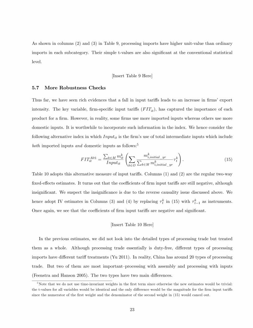
5.7 More Robustness Checks

Thus far, we have seen rich evidences that a fall in input tari¤s leads to an increase in �rms�export

intensity. The key variable, �rm-speci�c input tari¤s (FITit), has captured the importance of each

product for a �rm. However, in reality, some �rms use more imported inputs whereas others use more

domestic inputs. It is worthwhile to incorporate such information in the index. We hence consider the

following alternative index in which Inputit is the �rm�s use of total intermediate inputs which include

both imported inputs and domestic inputs as follows:5

FITAlt1it =

Pk2M m

kit

Inputit

Xk2O

mki;initial_yrP

k2M mki;initial_yr

�kt

!: (15)

Table 10 adopts this alternative measure of input tari¤s. Columns (1) and (2) are the regular two-way

�xed-e¤ects estimates. It turns out that the coe¢ cients of �rm input tari¤s are still negative, although

insigni�cant. We suspect the insigni�cance is due to the reverse causality issue discussed above. We

hence adopt IV estimates in Columns (3) and (4) by replacing �kt in (15) with �kt�1 as instruments.

Once again, we see that the coe¢ cients of �rm input tari¤s are negative and signi�cant.


In the previous estimates, we did not look into the detailed types of processing trade but treated

them as a whole. Although processing trade essentially is duty-free, di¤erent types of processing

imports have di¤erent tari¤ treatments (Yu 2011). In reality, China has around 20 types of processing

trade. But two of them are most important�processing with assembly and processing with inputs

(Feenstra and Hanson 2005). The two types have two main di¤erences.

5Note that we do not use time-invariant weights in the �rst term since otherwise the new estimates would be trivial:

the t-values for all variables would be identical and the only di¤erence would be the magnitude for the �rm input tari¤s

since the numerator of the �rst weight and the denominator of the second weight in (15) would cancel out.

23

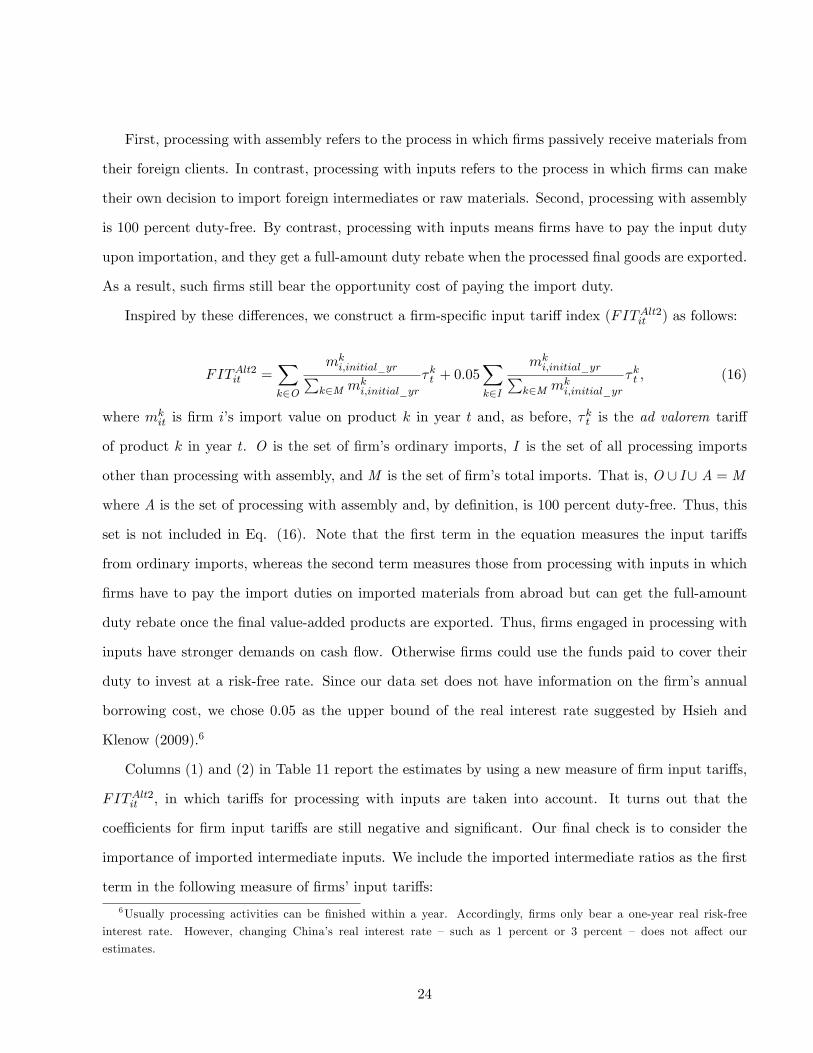
First, processing with assembly refers to the process in which �rms passively receive materials from

their foreign clients. In contrast, processing with inputs refers to the process in which �rms can make

their own decision to import foreign intermediates or raw materials. Second, processing with assembly

is 100 percent duty-free. By contrast, processing with inputs means �rms have to pay the input duty

upon importation, and they get a full-amount duty rebate when the processed �nal goods are exported.

As a result, such �rms still bear the opportunity cost of paying the import duty.

Inspired by these di¤erences, we construct a �rm-speci�c input tari¤ index (FITAlt2it ) as follows:

FITAlt2it =Xk2O

mki;initial_yrP

k2M mki;initial_yr

�kt + 0:05Xk2I

mki;initial_yrP

k2M mki;initial_yr

�kt ; (16)

where mkit is �rm i�s import value on product k in year t and, as before, �kt is the ad valorem tari¤

of product k in year t. O is the set of �rm�s ordinary imports, I is the set of all processing imports

other than processing with assembly, and M is the set of �rm�s total imports. That is, O [ I[ A = M

where A is the set of processing with assembly and, by de�nition, is 100 percent duty-free. Thus, this

set is not included in Eq. (16). Note that the �rst term in the equation measures the input tari¤s

from ordinary imports, whereas the second term measures those from processing with inputs in which

�rms have to pay the import duties on imported materials from abroad but can get the full-amount

duty rebate once the �nal value-added products are exported. Thus, �rms engaged in processing with

inputs have stronger demands on cash �ow. Otherwise �rms could use the funds paid to cover their

duty to invest at a risk-free rate. Since our data set does not have information on the �rm�s annual

borrowing cost, we chose 0.05 as the upper bound of the real interest rate suggested by Hsieh and

Klenow (2009).6

Columns (1) and (2) in Table 11 report the estimates by using a new measure of �rm input tari¤s,

FITAlt2it , in which tari¤s for processing with inputs are taken into account. It turns out that the

coe¢ cients for �rm input tari¤s are still negative and signi�cant. Our �nal check is to consider the

importance of imported intermediate inputs. We include the imported intermediate ratios as the �rst

term in the following measure of �rms�input tari¤s:

6Usually processing activities can be �nished within a year. Accordingly, �rms only bear a one-year real risk-free

interest rate. However, changing China�s real interest rate � such as 1 percent or 3 percent � does not a¤ect our

estimates.

24

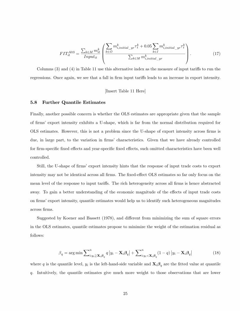
FITAlt3it =

Pk2M m

kit

Inputit

0BB@Xk2O

mki;initial_yr�

kt + 0:05

Xk2I

mki;initial_yr�

ktP

k2M mki;initial_yr

1CCA : (17)

Columns (3) and (4) in Table 11 use this alternative index as the measure of input tari¤s to run the

regressions. Once again, we see that a fall in �rm input tari¤s leads to an increase in export intensity.


5.8 Further Quantile Estimates

Finally, another possible concern is whether the OLS estimates are appropriate given that the sample

of �rms�export intensity exhibits a U-shape, which is far from the normal distribution required for

OLS estimates. However, this is not a problem since the U-shape of export intensity across �rms is

due, in large part, to the variation in �rms�characteristics. Given that we have already controlled

for �rm-speci�c �xed e¤ects and year-speci�c �xed e¤ects, such omitted characteristics have been well

controlled.

Still, the U-shape of �rms�export intensity hints that the response of input trade costs to export

intensity may not be identical across all �rms. The �xed-e¤ect OLS estimates so far only focus on the

mean level of the response to input tari¤s. The rich heterogeneity across all �rms is hence abstracted

away. To gain a better understanding of the economic magnitude of the e¤ects of input trade costs

on �rms�export intensity, quantile estimates would help us to identify such heterogeneous magnitudes

across �rms.

Suggested by Koener and Bassett (1978), and di¤erent from minimizing the sum of square errors

in the OLS estimates, quantile estimates propose to minimize the weight of the estimation residual as

follows:

�q = argminXn

i:yi=Xi�qq��yi �Xi�q��+Xn

i:yi<Xi�q(1� q)

��yi �Xi�q�� (18)

where q is the quantile level, yi is the left-hand-side variable and Xi�q are the �tted value at quantile

q. Intuitively, the quantile estimates give much more weight to those observations that are lower

25

than their �tted value at every quantile q. In this way, the estimates would be able to capture the

heterogenous behavior of �rms�export intensity.

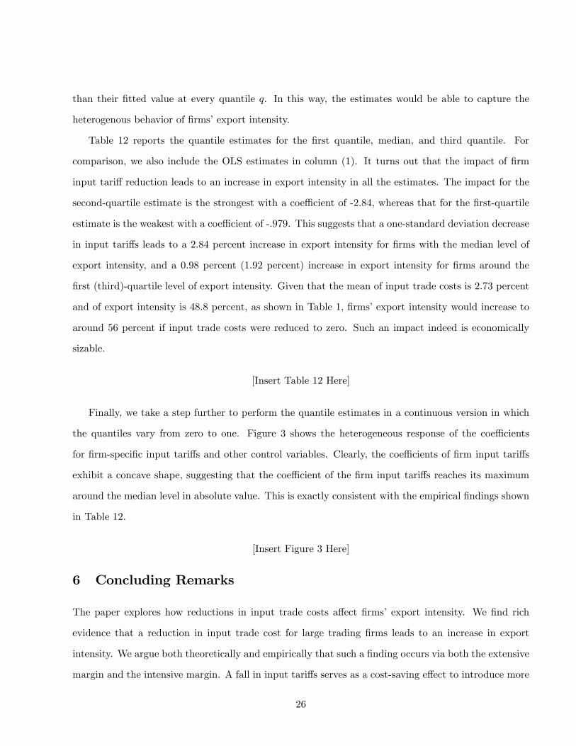
Table 12 reports the quantile estimates for the �rst quantile, median, and third quantile. For

comparison, we also include the OLS estimates in column (1). It turns out that the impact of �rm

input tari¤ reduction leads to an increase in export intensity in all the estimates. The impact for the

second-quartile estimate is the strongest with a coe¢ cient of -2.84, whereas that for the �rst-quartile

estimate is the weakest with a coe¢ cient of -.979. This suggests that a one-standard deviation decrease

in input tari¤s leads to a 2.84 percent increase in export intensity for �rms with the median level of

export intensity, and a 0.98 percent (1.92 percent) increase in export intensity for �rms around the

�rst (third)-quartile level of export intensity. Given that the mean of input trade costs is 2.73 percent

and of export intensity is 48.8 percent, as shown in Table 1, �rms�export intensity would increase to

around 56 percent if input trade costs were reduced to zero. Such an impact indeed is economically

sizable.


Finally, we take a step further to perform the quantile estimates in a continuous version in which

the quantiles vary from zero to one. Figure 3 shows the heterogeneous response of the coe¢ cients

for �rm-speci�c input tari¤s and other control variables. Clearly, the coe¢ cients of �rm input tari¤s

exhibit a concave shape, suggesting that the coe¢ cient of the �rm input tari¤s reaches its maximum

around the median level in absolute value. This is exactly consistent with the empirical �ndings shown

in Table 12.


6 Concluding Remarks

The paper explores how reductions in input trade costs a¤ect �rms�export intensity. We �nd rich

evidence that a reduction in input trade cost for large trading �rms leads to an increase in export

intensity. We argue both theoretically and empirically that such a �nding occurs via both the extensive

margin and the intensive margin. A fall in input tari¤s serves as a cost-saving e¤ect to introduce more

26

non-exporting �rms to export. More importantly, input tari¤ reduction also causes existing exporters

to increase their export intensity, since exporting sectors use more and better imported intermediate

inputs than domestic sectors. These two mechanisms are supported by the Chinese data.

Processing trade creates a quasi-natural experiment for us to understand the impact on export

intensity. The impact of input trade liberalization should not have any signi�cant impact on �rms�

export intensity for processing imports, since they are already duty-free. Although it is inappropriate

to conduct the standard di¤erence-in-di¤erence e¤ects, since the special tari¤ treatments in China

apply to our whole period, we instead check the role of processing imports directly in our data and

�nd strong empirical evidence for our �ndings.

The present paper is one of the �rst to explore the role of processing trade in Chinese �rms�export

share. The rich data set enables the determination of whether a �rm engages in processing trade and

the examination of the e¤ect of �rms�extent of processing trade engagement on export intensity. With

this information, �rm-speci�c input tari¤s were also constructed, as one of the �rst attempts in the

literature, which, in turn, enriches the understanding of the economic e¤ect of trade liberalization on

�rms�decision about sales.

27

References[1] Ahn, JaeBin, Amit Khandelwal, and Shang-Jin Wei (2011), "The Role of Intermediaries in Facil-

itating Trade," Journal of International Economics, 84(1), pp. 73-85.

[2] Amemiya, Takashi (1985), Advanced Econometrics, Cambridge, MA, Harvard University Press.

[3] Amiti, Mary, and Donald Davis (2011), "Trade, Firms, and Wages: Theory and Evidence," Reviewof Economic Studies 79, 1�36.

[4] Amiti, Mary, and Jozef Konings (2007), �Trade Liberalization, Intermediate Inputs, and Produc-tivity: Evidence from Indonesia,�American Economic Review 93, pp. 1611-1638.

[5] Amiti, Mary, and David Weinstein (2011), �Exports and Financial Shocks,�Quarterly Journal ofEconomics, 126 (4), 1841-1877.

[6] Anderson (1984)...

[7] Arkolakis, Costas, and Marc-Andreas Muendler(2010), "The Extensive Margin of Exporting Prod-ucts: A Firm-level Analysis," NBER Working Paper No. 16641.

[8] Bas, Maria, and Vanessa Strauss-Kahn (2011), "Does Importing more Inputs Raise Exports? FirmLevel Evidence from France," CEPII Working Paper, No. 2011-15.

[9] Bernard, Andrew, and Brad Jensen (1995), "Exporters, Jobs and Wages in U.S. Manufacturing,1976�1987," Brookings Papers on Economic Activity: Microeconomics, pp. 67�112.

[10] Bernard, Andrew, Jonathan Eaton, Bradford Jensen, and Samuel Kortum (2003), "Plants andProductivity in International Trade," American Economic Review 93 (5), pp. 1628-90.

[11] Bernard, Andrew, Brad Jensen and Peter Schott (2009), "Importers, Exporters, and Multination-als: A Portrait of Firms in the U.S. that Trade Goods," in: Duune, T. Jensen J.B., Robert, M.J.(Eds.), Producer Dynamics: New Evidences from Micro Data, University of Chicago Press.

[12] Bernard, Andrew, Brad Jensen and Peter Schott (2010), "Multiple-Product Firms and ProductSwitching", American Economic Review 100(1), pp. 70-97.

[13] Bonaccorsi, Andrea (1992), "On the Relationship between Firm Size and Export Intensity," Jour-nal of International Business Studies 23(4), pp. 605-35.

[14] Brandt, Loren, Johannes Van Biesebroeck, and Yifan Zhang (2012), "Creative Accounting orCreative Destruction? Firm-Level Productivity Growth in Chinese Manufacturing," Journal ofDevelopment Economics 97(2), pp.339-51.

[15] Brooks, Eileen (2006), "Why don�t �rms export more? Product quality and Colombian plants,"Journal of Development Economics 80(1), pp. 160-78.

[16] Cameron, Colin and Pravin Trivedi (2005), Microeconometrics: Methods and Applications, Cam-bridge University Press.

[17] Dai, Mi, Madhura Maitra, and Miaojie Yu (2012), "Unexceptional Exporter Performance inChina? The Role of Processing Trade", mimeo, Peking University.

[18] De Loecker, Jan, and Frederic Warzynski (2012), "Markups and Firm-Level Export Status,"American Economic Review, forthcoming.

28

[19] Eaton Jonathan, Samuel Kortum, and Francis Kramarz (2011), "An Anatomy of InternationalTrade: Evidence from French Firms," Econometrica 79(5), pp. 1453-98.

[20] Feenstra, Robert, and Gordon Hanson (2005), �Ownership and Control in Outsourcing to China:Estimating the Property-Rights Theory of the Firm,�Quarterly Journal of Economics 120(2), pp.729-762.

[21] Feenstra, Robert, Zhiyuan Li, and Miaojie Yu (2011), "Export and Credit Constraints underIncomplete Information: Theory and Empirical Investigation from China", NBERWorking Paper,No. 16940.

[22] Feng, Ling, Zhiyuan Li, and Doborah Swensen (2012), "The Connection between Imported In-termediate Inputs and Exports: Evidence from Chinese Firms", mimeo, University of California,Davis.

[23] Ge Ying, Huiwen Lai, and Susan Chun Zhu (2011), "Intermediates Imports and Gains from TradeLiberalization," mimeo, University of International and Business Economics, China.

[24] Greenaway David, Nuso Sousa and Katherine Wakelin (2004), "Do domestic �rms learn to exportfrom multinationals?" European Journal of Political Economy 20, pp. 1027-43.

[25] Grossman, Gene, and Elhanan Helpman (1994), "Protection for Sales," American Economic Re-view 84(4), pp. 833-50.

[26] Hallak, C. Juan (2006), "Product Quality and the Direction of Trade," Journal of InternationalEconomics, 68(1), pp. 238-265,

[27] Heckman, James (1979), "Sample Selection Bias as a Speci�cation Error," Econometrica, 47(1),pp. 153-61.

[28] Helpern, Laszlo, Miklos Koren, and Adam Szeidl (2010), "Imported Inputs and Productivity,"Mimeo, University of California, Berkeley.

[29] Hirschman, A. O.(1958), The Strategy of Economic Development, Yale University Press.

[30] Hsieh, Chang-Tai and Peter J. Klenow (2009), "Misallocation and Manufacturing TFP in Chinaand India," Quarterly Journal of Economics, 124(4), pp. 1403-48.

[31] Imbens, G. (2004), "Nonparametric Estimation of Average Treatment E¤ects Under Exogeneity:A Review," Review of Economics and Statistics 86(1): pp. 4�29.

[32] Kleibergen, Frank, and Richard Paap (2006), "Generalized Reduced Rank Tests Using the SingularValue Decomposition," Journal of Econometrics 133(1), pp. 97-126.

[33] Koener, R., and G. Bassett (1978), "Regression Quantiles," Econometrica 46, pp. 107-12.

[34] Levchenko, Andrei A. (2007), "Institutional quality and international trade," Review of EconomicStudies 74, 791�819.

[35] Lu, Dan (2011), "Exceptional Exporter Performance? Evidence from Chinese ManufacturingFirms," mimeo, University of Chicago.

[36] Lu, Jiangyong, Yi Lu, and Zhigang Tao (2010), "Exporting Behavior of Foreign A¢ liates: Theoryand Evidence", Journal of International Economics 81(2), pp. 197-205.

[37] Melitz, Marc (2003), "The Impact of Trade on Intra-industry Reallocations and Aggregate Indus-try Productivity," Econometrica 71(6), pp. 1695-1725.

29

[38] Olley, Steven, and Ariel Pakes (1996), "The Dynamics of Productivity in the TelecommunicationsEquipment Industry," Econometrica 64(6), pp. 1263-97.

[39] Soderbery, Anson (2012), "The Competitive E¤ects of Heterogenous Firms Facing Capacity Con-straints under International Trade," mimeo, Purdue University.

[40] Tre�er, Daniel (2004), �The Long and Short of the Canada-U.S. Free Trade Agreement,�AmericanEconomics Review 94(3), pp. 870-95.

[41] Topalova, Petia and Amit Khandelwal (2011), "Trade Liberalization and Firm Productivity: TheCase of India," Review of Economics and Statistics 93(3), pp. 995-1009.

[42] Tybout, James (2000),"Manufacturing Firms in Developing Countries: How Well Do They Do,and Why?�Journal of Economic Literature 38(1), pp. 11-44.

[43] Vannoorenberghe, G. (2012), "Firm-Level Volatility and Exports," Journal of International Eco-nomics 86(1), pp. 57-67.

[44] Yu, Miaojie (2011), "Processing Trade, Tari¤ Reductions, and Firm Productivity: Evidence fromChinese Product," mimeo, Peking University.

[45] Yu, Miaojie, and Wei Tian (2012), �China�s Processing Trade: A Firm-Level Analysis,� in HuwMcMay and Ligang Song (eds.) Rebalancing and Sustaining Growth in China, Australian NationalUniversity E-press, pp. 111-48.

30

Table 1A: Comparison of the Merged and Full-sample Trade DataPercentage of Firms Merged Sample Full SampleOrdinary Importers 38.1% 27.3%Processing Importers 61.9% 72.7%

Table 1B: Comparison of the Merged and Full-sample Production DataVariables Merged Data Full-sample Data Percentage

Mean Min. Max. Mean Min. Max.Sales 150,071 5000 1.57e+08 85,065 5000 1.57e+08 25.4%Exports 53,314 0 1.52e+08 16,544 0 1.52e+08 52.8%Number of Employees 478 10 157,213 274 10 165,878 23.7%

31

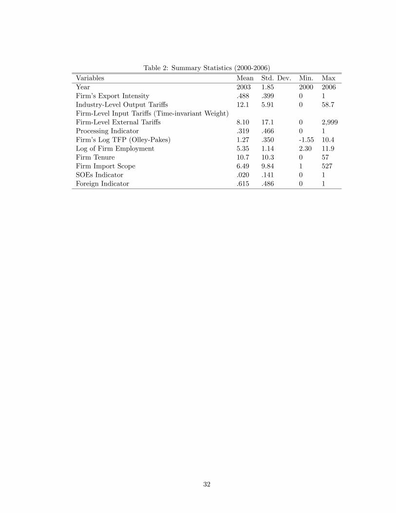
Table 2: Summary Statistics (2000-2006)Variables Mean Std. Dev. Min. MaxYear 2003 1.85 2000 2006Firm�s Export Intensity .488 .399 0 1Industry-Level Output Tari¤s 12.1 5.91 0 58.7Firm-Level Input Tari¤s (Time-invariant Weight)Firm-Level External Tari¤s 8.10 17.1 0 2,999Processing Indicator .319 .466 0 1Firm�s Log TFP (Olley-Pakes) 1.27 .350 -1.55 10.4Log of Firm Employment 5.35 1.14 2.30 11.9Firm Tenure 10.7 10.3 0 57Firm Import Scope 6.49 9.84 1 527SOEs Indicator .020 .141 0 1Foreign Indicator .615 .486 0 1

32

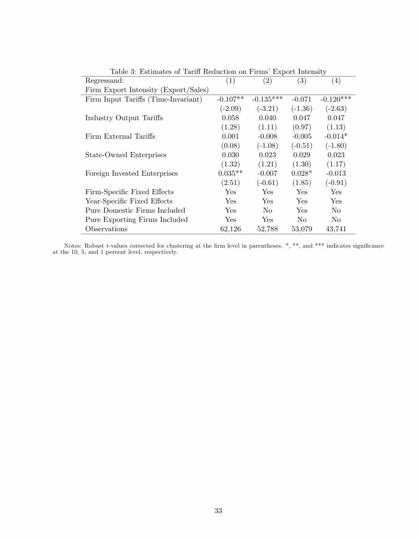
Table 3: Estimates of Tari¤ Reduction on Firms�Export IntensityRegressand: (1) (2) (3) (4)Firm Export Intensity (Export/Sales)Firm Input Tari¤s (Time-Invariant) -0.107** -0.135*** -0.071 -0.120***

(-2.09) (-3.21) (-1.36) (-2.63)Industry Output Tari¤s 0.058 0.040 0.047 0.047

(1.28) (1.11) (0.97) (1.13)Firm External Tari¤s 0.001 -0.008 -0.005 -0.014*

(0.08) (-1.08) (-0.51) (-1.80)State-Owned Enterprises 0.030 0.023 0.029 0.023

(1.32) (1.21) (1.30) (1.17)Foreign Invested Enterprises 0.035** -0.007 0.028* -0.013

(2.51) (-0.61) (1.85) (-0.91)Firm-Speci�c Fixed E¤ects Yes Yes Yes YesYear-Speci�c Fixed E¤ects Yes Yes Yes YesPure Domestic Firms Included Yes No Yes NoPure Exporting Firms Included Yes Yes No NoObservations 62,126 52,788 53,079 43,741

Notes: Robust t-values corrected for clustering at the �rm level in parentheses. *, **, and *** indicates signi�canceat the 10, 5, and 1 percent level, respectively.

33

Table 4: Instrumental Variable Estimates of Tari¤ Reduction on Firms�Export IntensityRegressand: Export Intensity Log Exports Log Ordinary Exports

over Domestic Sales over Domestic Sales(1) (2) (3) (4)

Firm Input Tari¤s (Time-Invariant) -1.40*** -1.34*** -8.98*** -3.68**(-8.22) (-7.65) (-6.14) (-3.08)

Industry Output Tari¤s .623*** .765*** 4.75*** 6.95*(14.43) (15.01) (10.83) (17.49)

Firm External Tari¤s -.027** -.018 -.109 -.172*(-2.00) (-1.36) (-1.40) (-2.18)

State-Owned Enterprises -.075*** -.127*** -.948*** -.821**(-7.79) (-10.17) (-8.73) (-8.04)

Foreign Invested Enterprises .146*** .155*** .811*** -.058*(32.00) (31.93) (21.22) (1.65)

Firm TFP (Olley-Pakes) -.113*** -.755*** -.120***(-17.28) (-13.52) (-4.67)

Firm Size .020*** -.003 -.415***(13.82) (-.27) (-32.94)

Kleibergen-Paap rk LM statistic 129.4y 114.9y 89.51y 102.9y

Kleibergen-Paap Wald rk F statistic 235.9y 195.8y 472.1y 191.7y

Industry-Speci�c Fixed E¤ects Yes Yes Yes YesYear-Speci�c Fixed E¤ects Yes Yes Yes YesPure Domestic Firms Included Yes Yes No YesPure Exporter Firms Included Yes Yes No YesObservations 56,548 46,963 33,442 35,338R-Squared 0.19 0.19 0.17 0.10

First-Stage RegressionsIV: One Lag of Firm Input Tari¤s 0.573*** 0.576*** 0.606*** .585***(with Time Invariant Weight) (15.36) (13.99) (21.72) (13.84)

[235.9] [195.7] [471.5] [191.5]

Notes: Robust t-values corrected for clustering at the �rm level in parentheses. *, **, and *** indicates signi�canceat the 10, 5, and 1 percent level, respectively. Numbers in brackets are F-values.

34

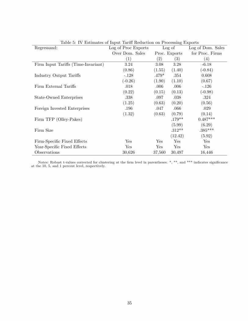
Table 5: IV Estimates of Input Tari¤ Reduction on Processing ExportsRegressand: Log of Proc Exports Log of Log of Dom. Sales

Over Dom. Sales Proc. Exports for Proc. Firms(1) (2) (3) (4)

Firm Input Tari¤s (Time-Invariant) 3.24 3.08 3.28 -6.18(0.86) (1.55) (1.40) (-0.84)

Industry Output Tari¤s -.128 .479* .354 0.608(-0.26) (1.90) (1.10) (0.67)

Firm External Tari¤s .018 .006 .006 -.126(0.22) (0.15) (0.13) (-0.98)

State-Owned Enterprises .338 .097 .038 .324(1.25) (0.63) (0.20) (0.56)

Foreign Invested Enterprises .196 .047 .066 .029(1.32) (0.63) (0.79) (0.14)

Firm TFP (Olley-Pakes) .179** 0.487***(5.99) (6.29)

Firm Size .312** .385***(12.42) (5.92)

Firm-Speci�c Fixed E¤ects Yes Yes Yes YesYear-Speci�c Fixed E¤ects Yes Yes Yes YesObservations 30,626 37,560 30,497 16,446


35

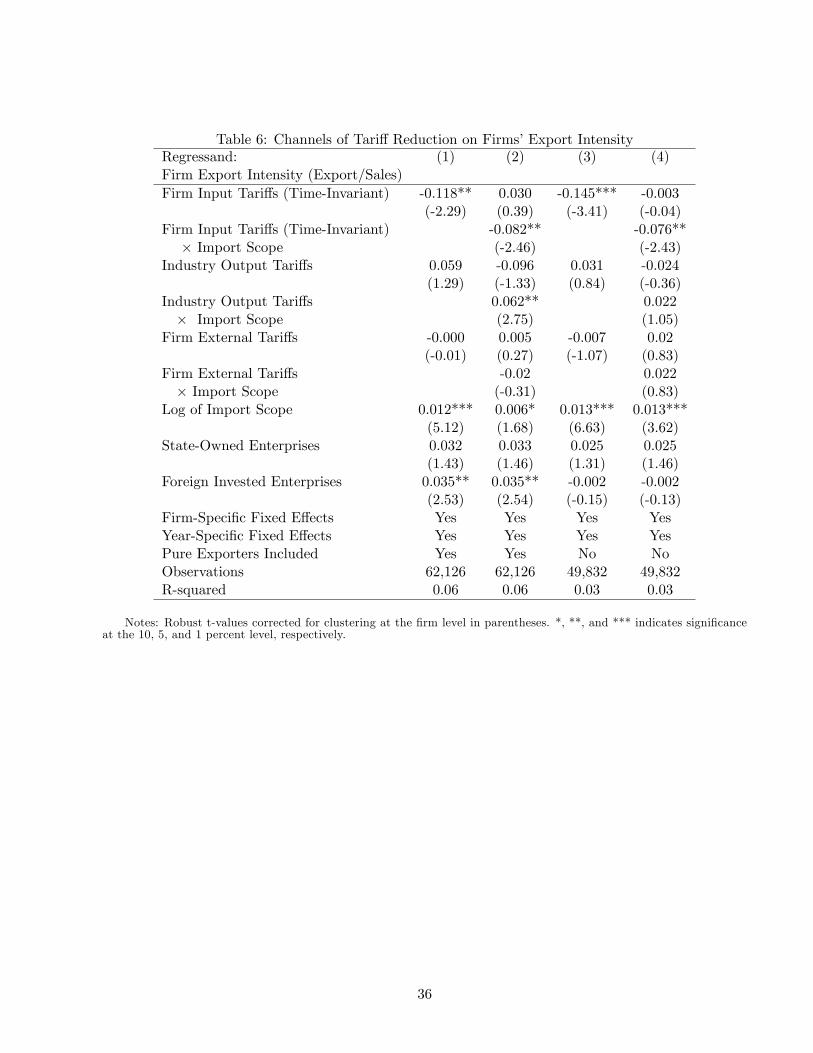
Table 6: Channels of Tari¤ Reduction on Firms�Export IntensityRegressand: (1) (2) (3) (4)Firm Export Intensity (Export/Sales)Firm Input Tari¤s (Time-Invariant) -0.118** 0.030 -0.145*** -0.003

(-2.29) (0.39) (-3.41) (-0.04)Firm Input Tari¤s (Time-Invariant) -0.082** -0.076**� Import Scope (-2.46) (-2.43)

Industry Output Tari¤s 0.059 -0.096 0.031 -0.024(1.29) (-1.33) (0.84) (-0.36)

Industry Output Tari¤s 0.062** 0.022� Import Scope (2.75) (1.05)

Firm External Tari¤s -0.000 0.005 -0.007 0.02(-0.01) (0.27) (-1.07) (0.83)

Firm External Tari¤s -0.02 0.022� Import Scope (-0.31) (0.83)

Log of Import Scope 0.012*** 0.006* 0.013*** 0.013***(5.12) (1.68) (6.63) (3.62)

State-Owned Enterprises 0.032 0.033 0.025 0.025(1.43) (1.46) (1.31) (1.46)

Foreign Invested Enterprises 0.035** 0.035** -0.002 -0.002(2.53) (2.54) (-0.15) (-0.13)

Firm-Speci�c Fixed E¤ects Yes Yes Yes YesYear-Speci�c Fixed E¤ects Yes Yes Yes YesPure Exporters Included Yes Yes No NoObservations 62,126 62,126 49,832 49,832R-squared 0.06 0.06 0.03 0.03


36

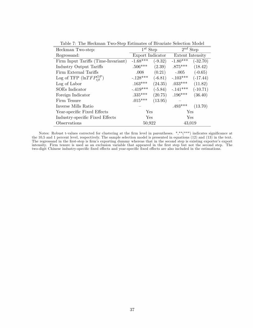
Table 7: The Heckman Two-Step Estimates of Bivariate Selection ModelHeckman Two-step: 1st Step 2nd StepRegressand: Export Indicator Extent IntensityFirm Input Tari¤s (Time-Invariant) -1.68*** (-9.32) -1.80*** (-32.70)Industry Output Tari¤s .506*** (2.39) .875*** (18.42)Firm External Tari¤s .008 (0.21) -.005 (-0.65)Log of TFP (lnTFPOPijt ) -.128*** (-6.81) -.103*** (-17.44)Log of Labor .163*** (24.35) .033*** (11.82)SOEs Indicator -.419*** (-5.84) -.141*** (-10.71)Foreign Indicator .335*** (20.75) .196*** (36.40)Firm Tenure .015*** (13.95) �Inverse Mills Ratio � .493*** (13.70)Year-speci�c Fixed E¤ects Yes YesIndustry-speci�c Fixed E¤ects Yes YesObservations 50,922 43,019

Notes: Robust t-values corrected for clustering at the �rm level in parentheses. *,**(***) indicates signi�cance atthe 10,5 and 1 percent level, respectively. The sample selection model is presented in equations (12) and (13) in the text.The regressand in the �rst-step is �rm�s exporting dummy whereas that in the second step is existing exporter�s exportintensity. Firm tenure is used as an exclusion variable that appeared in the �rst step but not the second step. Thetwo-digit Chinese industry-speci�c �xed e¤ects and year-speci�c �xed e¤ects are also included in the estimations.

37

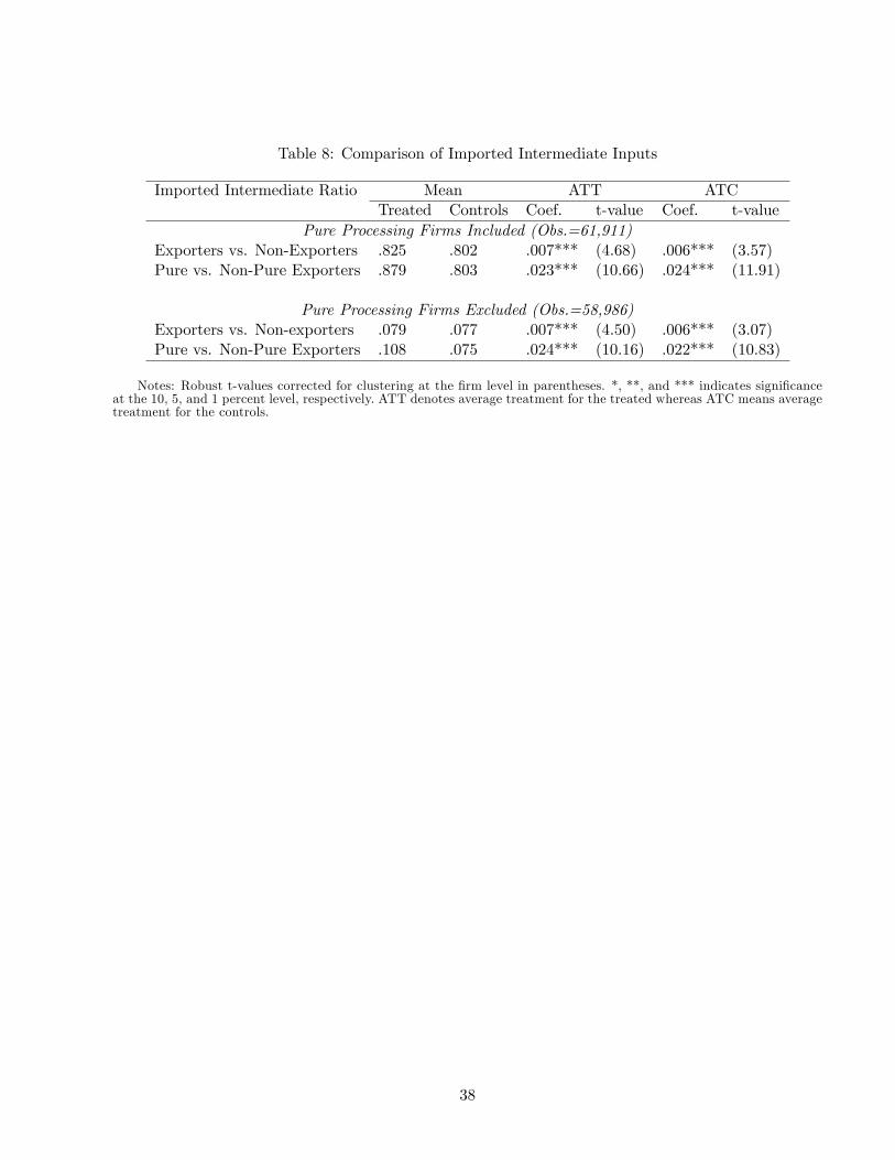
Table 8: Comparison of Imported Intermediate Inputs

Imported Intermediate Ratio Mean ATT ATCTreated Controls Coef. t-value Coef. t-value

Pure Processing Firms Included (Obs.=61,911)Exporters vs. Non-Exporters .825 .802 .007*** (4.68) .006*** (3.57)Pure vs. Non-Pure Exporters .879 .803 .023*** (10.66) .024*** (11.91)

Pure Processing Firms Excluded (Obs.=58,986)Exporters vs. Non-exporters .079 .077 .007*** (4.50) .006*** (3.07)Pure vs. Non-Pure Exporters .108 .075 .024*** (10.16) .022*** (10.83)

Notes: Robust t-values corrected for clustering at the �rm level in parentheses. *, **, and *** indicates signi�canceat the 10, 5, and 1 percent level, respectively. ATT denotes average treatment for the treated whereas ATC means averagetreatment for the controls.

38

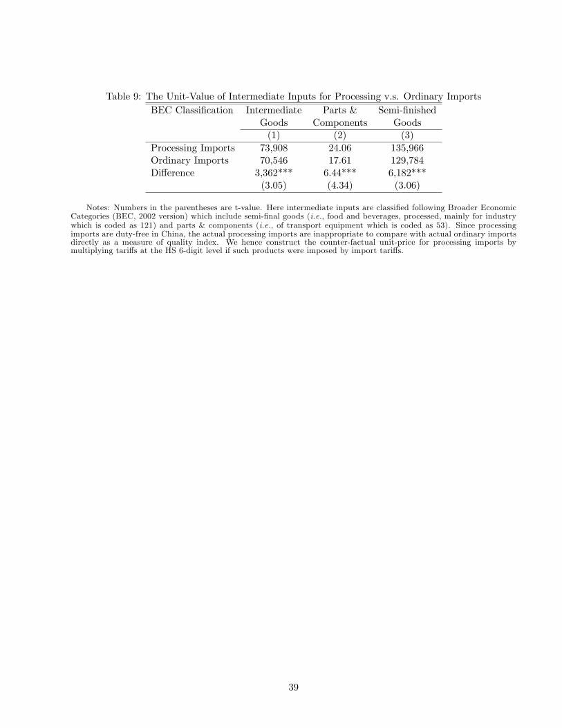
Table 9: The Unit-Value of Intermediate Inputs for Processing v.s. Ordinary ImportsBEC Classi�cation Intermediate Parts & Semi-�nished

Goods Components Goods(1) (2) (3)

Processing Imports 73,908 24.06 135,966Ordinary Imports 70,546 17.61 129,784Di¤erence 3,362*** 6.44*** 6,182***

(3.05) (4.34) (3.06)

Notes: Numbers in the parentheses are t-value. Here intermediate inputs are classi�ed following Broader EconomicCategories (BEC, 2002 version) which include semi-�nal goods (i.e., food and beverages, processed, mainly for industrywhich is coded as 121) and parts & components (i.e., of transport equipment which is coded as 53). Since processingimports are duty-free in China, the actual processing imports are inappropriate to compare with actual ordinary importsdirectly as a measure of quality index. We hence construct the counter-factual unit-price for processing imports bymultiplying tari¤s at the HS 6-digit level if such products were imposed by import tari¤s.

39

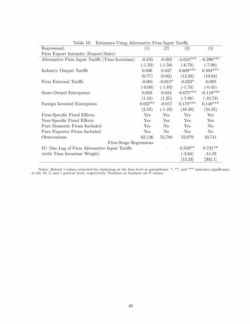
Table 10: Estimates Using Alternative Firm Input Tari¤sRegressand: (1) (2) (3) (4)Firm Export Intensity (Export/Sales)Alternative Firm Input Tari¤s (Time-Invariant) -0.245 -0.262 -4.824*** -6.296***

(-1.32) (-1.59) (-6.70) (-7.09)Industry Output Tari¤s 0.036 0.027 0.609*** 0.504***

(0.77) (0.62) (13.93) (10.94)Firm External Tari¤s -0.001 -0.015* -0.023* -0.005

(-0.09) (-1.83) (-1.74) (-0.45)State-Owned Enterprises 0.033 0.024 -0.075*** -0.110***

(1.44) (1.25) (-7.86) (-10.73)Foreign Invested Enterprises 0.037** -0.017 0.178*** 0.140***

(2.53) (-1.23) (48.29) (34.35)Firm-Speci�c Fixed E¤ects Yes Yes Yes YesYear-Speci�c Fixed E¤ects Yes Yes Yes YesPure Domestic Firms Included Yes No Yes NoPure Exporter Firms Included Yes No Yes NoObservations 62,126 52,788 53,079 43,741

First-Stage RegressionsIV: One Lag of Firm Alternative Input Tari¤s � � 0.559** 0.731**(with Time Invariant Weight) (-3.64) -14.23

[13.23] [202.1]


40

Table 11: Estimates with Alternative Measaure of Firm Input Tari¤sMeasured Weight in Firm Input Tari¤s Imported Intermediate Inputs Total InputsRegressand: Firm Export Intensity (1) (2) (3) (4)Firm Input Tari¤s -0.133* -0.176** -0.859*** -0.833***(with Tari¤s for Processing with Inputs) (-1.64) (-2.54) (-4.43) (-4.70)Industry Output Tari¤s 0.048 0.039 0.034 0.028

(1.15) (1.04) (0.80) (0.73)Firm External Tari¤s -0.007 -0.013*** -0.005 -0.009*

(-1.50) (-2.86) (-0.94) (-1.92)State-Owned Enterprises 0.020 0.019 0.026 0.025

(1.00) (1.08) (1.29) (1.46)Foreign Invested Enterprises 0.032** -0.015 0.034*** -0.017

(2.47) (-1.24) (2.61) (-1.34)Firm TFP (Olley-Pakes) -0.025*** -0.045*** -0.023*** -0.053***

(-6.07) (-10.86) (-3.88) (-9.25)Firm Size 0.023*** 0.017*** 0.019*** 0.014***

(6.73) (5.05) (5.39) (4.08)Firm-Speci�c Fixed E¤ects Yes Yes Yes YesYear-Speci�c Fixed E¤ects Yes Yes Yes YesObservations 68,903 48,923 63,184 45,367R-squared 0.01 0.01 0.01 0.01


41

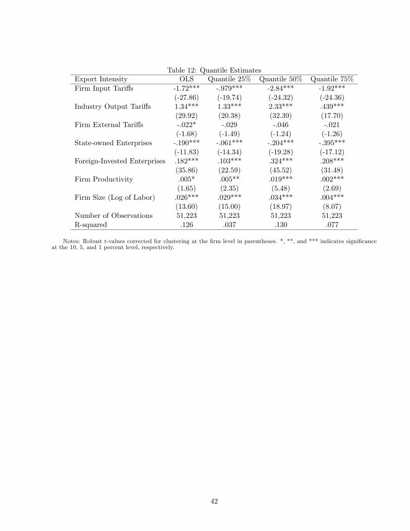
Table 12: Quantile EstimatesExport Intensity OLS Quantile 25% Quantile 50% Quantile 75%Firm Input Tari¤s -1.72*** -.979*** -2.84*** -1.92***

(-27.86) (-19.74) (-24.32) (-24.36)Industry Output Tari¤s 1.34*** 1.33*** 2.33*** .439***

(29.92) (20.38) (32.39) (17.70)Firm External Tari¤s -.022* -.029 -.046 -.021

(-1.68) (-1.49) (-1.24) (-1.26)State-owned Enterprises -.190*** -.061*** -.204*** -.395***

(-11.83) (-14.34) (-19.28) (-17.12)Foreign-Invested Enterprises .182*** .103*** .324*** .208***

(35.86) (22.59) (45.52) (31.48)Firm Productivity .005* .005** .019*** .002***

(1.65) (2.35) (5.48) (2.69)Firm Size (Log of Labor) .026*** .029*** .034*** .004***

(13.60) (15.00) (18.97) (8.07)Number of Observations 51,223 51,223 51,223 51,223R-squared .126 .037 .130 .077


42

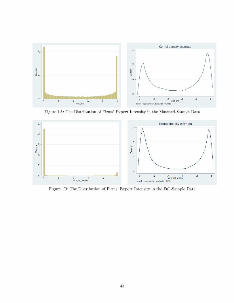
05

10D

ensi

ty

0 .2 .4 .6 .8 1exp_int

.51

1.5

2D

ensi

ty

0 .2 .4 .6 .8 1exp_int

kernel = epanechnikov, bandwidth = 0.0310

Kernel density estimate

Figure 1A: The Distribution of Firms�Export Intensity in the Matched-Sample Data

Figure 1B: The Distribution of Firms�Export Intensity in the Full-Sample Data

43

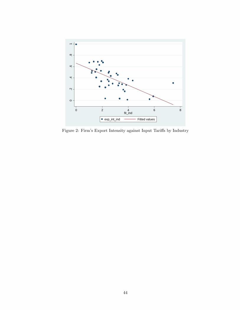
0.2

.4.6

.81

0 2 4 6 8fit_ind

exp_int_ind Fitted values

Figure 2: Firm�s Export Intensity against Input Tari¤s by Industry

44

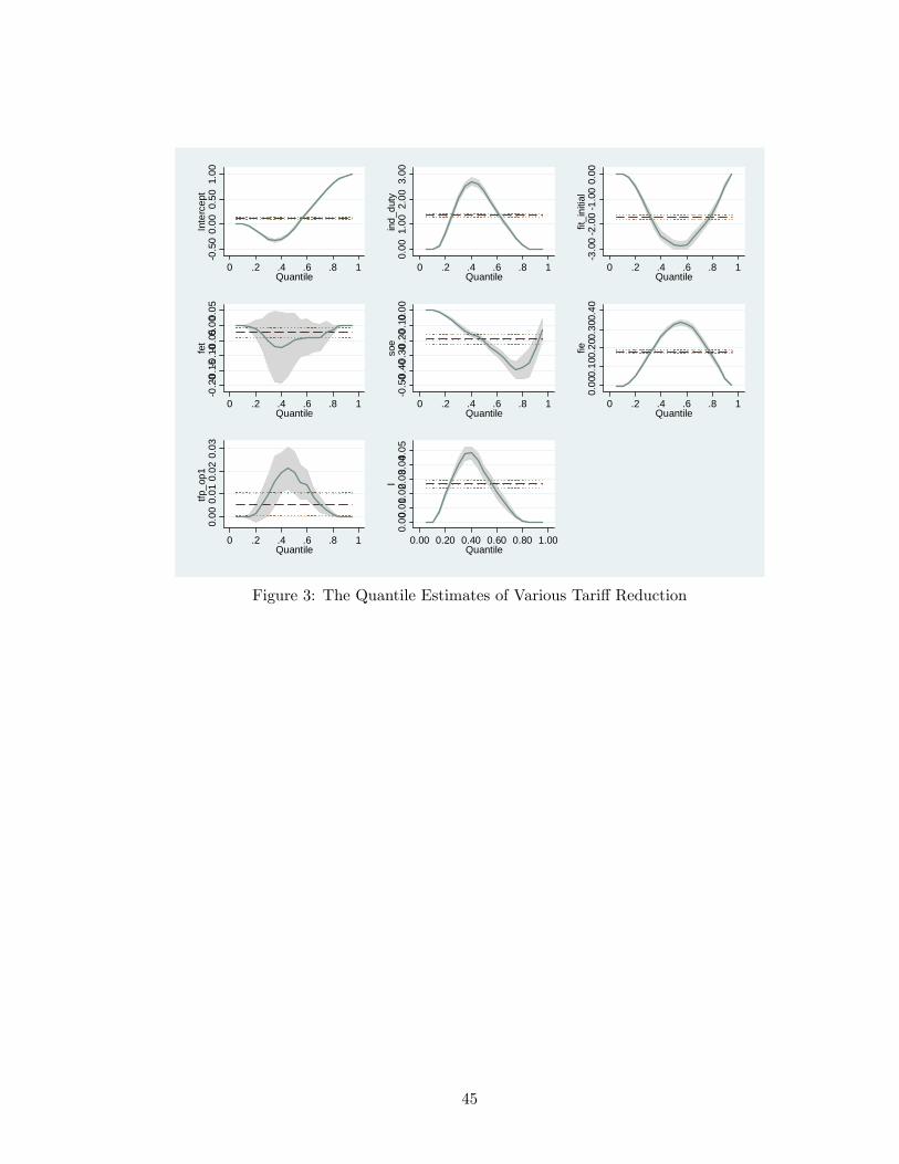
0.5

00.

000.

501.

00In

terc

ept

0 .2 .4 .6 .8 1Quantile

0.00

1.00

2.00

3.00

ind_

duty

0 .2 .4 .6 .8 1Quantile

3.0

02

.00

1.0

00.

00fit

_ini

tial

0 .2 .4 .6 .8 1Quantile

0.2

00.1

50.1

00.0

50.00

0.05

fet

0 .2 .4 .6 .8 1Quantile

0.5

00.4

00.3

00.2

00.1

00.00

soe

0 .2 .4 .6 .8 1Quantile

0.00

0.10

0.20

0.30

0.40

fie

0 .2 .4 .6 .8 1Quantile

0.00

0.01

0.02

0.03

tfp_o

p1

0 .2 .4 .6 .8 1Quantile

0.000

.010.

020.0

30.040

.05

l

0.00 0.20 0.40 0.60 0.80 1.00Quantile

Figure 3: The Quantile Estimates of Various Tari¤ Reduction

45

7 Appendix

7.1 Appendix A1: Proof of Proposition 1

Since dBrd� = �Ar

S2F

dSFd� < 0;8r = d; x, and �rms�domestic pro�t is:

�d(') =Eh�(w��'P )��1(1 +B��1d )

(1��)(��1)��1 � f;

we have d�d(')d� = @�d(')@Bd

dBdd� < 0 since @�d(')@Bd

> 0. Similarly, given �rms�pro�t in the foreign market is:

�x(') =n�1��

�Ef (w

��'P )��1(1 +B��1x )(1��)(��1)

��1 � fx;

we have d�x(')d� = @�x(')

@BxdBxd� < 0. Therefore a decrease in input trade costs leads to an increase in

�rms�pro�t.d�(')

d�=d�d(')

d�+d�x(')

d�< 0:

(QED)

7.2 Appendix A2: Proof of Proposition 2To show that a decease in �rm input trade costs leads to an increase in �rms�export intensity, we needto show d(1=&)

d� > 0. Given

1

�= 1 +

Ehn�1��Ef

1 +B��1d

1 +B��1x

! (1��)(��1)��1

;

we have:

d(1=&)

d�=

Ehn�1��Ef

(1� �)(� � 1)� � 1

1 +B��1d

1 +B��1x

! (1��)(��1)��1 �1

�(� � 1)

��1 +B��1x

�B��2d

dBdd� �

�1 +B��1d

�B��2x

dBxd�

��1 +B��1x

�2 :

Since dBrd� = �Ar

S2F

dSFd� < 0;8r = d; x, we know that d(1=&)d� > 0 is equivalent to:�

1 +B��1x

�B��2d Ad <

�1 +B��1d

�B��2x Ax;

or, 1 +B��1d

1 +B��1x

! 1��1

>AdAx

given Bd=Bx = Ad=Ax from Br = Ar=SF : By simplifying, the expression above is equivalent to:

Ax > Ad:

(QED)

46

7.3 Appendix B: Method of Matching Firm and Trade DataIt is not an easy task to match �rm-level production and transaction-level trade data sets since �rms�identi�cation numbers are totally di¤erent in the two data sets. For example, the length of the �rm�sID variable in the transaction-level trade data set is ten digits, whereas in the �rm-level data set itonly has nine digits.

To address this challenge, following Yu and Tian (2012), we use two ways to match these two datasets. First, we match the two data sets by �rm name and year. That is, if a �rm has an exact Chinesename in both data sets in a particular year, they should be an identical �rm.7 As a result, the numberof matching �rms is 83,679 in total by using the raw production data set, and reduced to 69,623 intotal by using the more accurate �ltered production data set as described in the text.

Equally important, we then use another matching technique to serve as a supplement. Here werely on two other common variables to identify �rms, namely, zip code and the last seven digits ofthe �rm�s phone number. The rationale is that �rms should have a unique phone number within apostal district. Although this method seems straightforward, subtle technical and practical di¢ cultiesstill remain.8 Therefore, we use the last seven digits of the phone number to serve as a proxy for �rmidenti�cation.9

A �rm could be missing its name information in either the trade or production data set. Similarly,a �rm could lose information on phone and/or zip code. To secure that our matched data set cancover as many common �rms as possible, we include the observations in the matched data set if a �rmoccurred in either the name-adopted matched data set or the phone-and-post-adopted matched dataset. As a result, the number of matched �rms increases to 90,558 when the raw production data setis used, as shown in column (7) in Table A1. By way of comparison, such a matching performanceis of the same magnitude as (or even better than) other similar studies.10 Finally, if we adopt themore rigorous �ltered production data to merge with the �rm data, the matched data set ends up with76,823 �rms in total, as shown in the last column in Table A1.

7The year variable is necessary to use for an auxiliary identi�cation variable since some �rms could change their name

in di¤erent years and newcomers could possibly take their original name.8For example, the phone numbers in the product-level trade data include both area phone codes and a hyphen, whereas

those in the �rm-level production data do not.9This approach is adopted for two reasons: (1) during 2000�2006, some large Chinese cities changed their phone

number digits from seven to eight, which usually added one more digit at the start of the number. Therefore, sticking

to the last seven digits of the number would not confuse the �rms� identi�cation; and (2) in the original data set, the

phone number is de�ned as a string of characters with the phone zip code. However, it is inappropriate to de-string

such characters to numerals since a hyphen bar is used to connect the zip code and the phone number. Using the last

seven-digit substring solves this problem neatly.10For example, Ge et al. (2011) use the same data sets and similar matching techniques but end up with 86,336 matched

�rms in total.

47

Table A1: Matched Statistics�Number of FirmsYear Trade Data Production Data Matched Data

Transactions Firms Raw Filtered w/ Raw w/ Filtered w/ Raw w/ FilteredFirms Firms Firms Firms Firms Firms

(1) (2) (3) (4) (5) (6) (7) (8)2000 10,586,696 80,232 162,883 83,628 18,580 12,842 21,665 15,7482001 12,667,685 87,404 169,031 100,100 21,583 15,645 25,282 19,0912002 14,032,675 95,579 181,557 110,530 24,696 18,140 29,144 22,2912003 18,069,404 113,147 196,222 129,508 28,898 21,837 34,386 26,9302004 21,402,355 134,895 277,004 199,927 44,338 35,007 50,798 40,7112005 24,889,639 136,604 271,835 198,302 44,387 34,958 50,426 40,3872006 16,685,377 197,806 301,960 224,854 53,748 42,833 59,133 47,591All Years 118,333,831 286,819 615,951 438,165 83,679 69,623 90,558 76,946

Notes: Column (1) reports the number of observations of HS eight-digit monthly transaction-level trade data fromChina�s General Administration of Customs by year. Column (2) reports number of �rms covered in the transaction-level trade data by year. Column (3) reports number of �rms covered in the �rm-level production data set compiled byChina�s National Bureau of Statistics without any �ltering and cleaning. By contrast, Column (4) presents number of�rms covered in the �rm-level production dataset with careful �lter according to the requirements of GAAP. Accordingly,Column (5) reports the number of matched �rms using exactly identical company names in both trade dataset and rawproduction dataset. By contrast, Column (6) reports the number of matched �rms using exactly identical company namesin both the trade data set and the �ltered production data set. Finally, Column (7) reports the number of matched �rmsusing exactly identical company�names and exactly identical zip code and phone numbers in both the trade data setand the raw production data set. By contrast, Column (8) reports the number of matched �rms using exactly identicalcompany names and exactly identical zip code and phone numbers in both the trade data set and the �ltered productiondata set.

48

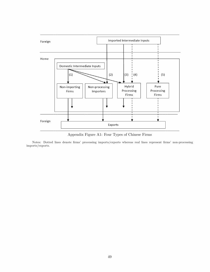
Appendix Figure A1: Four Types of Chinese Firms

Notes: Dotted lines denote �rms� processing imports/exports whereas real lines represent �rms� non-processingimports/exports.

49

Documents

Export Intensity and Input Trade Liberalization: Evidence ... · We thank Andrew Bernard, Robert Feenstra, Gordon Hanson, Samuel Kortum, Zhiyuan Li, Justin Lin, Robert Staiger, James