Exploring Peat Thickness Variability Using VLF Method Peat Thickness.pdf · In turn, in the area of deep peat, it is statistically similar until 4.72 meter and starts to show differences

142

INTRODUCTION

Peatlands have extremely relevant functions for the global climate, biosphere, and hydrology. A better knowledge of peat stocks is one of the prerequisites for science-based wetland manage-ment. Improper use of peatlands as well as its drainage and transformation have been reported widely. Tidal peat land in Pulau Rimau, South Su-matra (Armanto, 2014) and the Mega Rice Estate Project in Kalimantan (Limin, 2006) are examples of peat management failure. However, peat fire is probably the greatest challenge. Unlike common fire, peat fires cause much more carbon to be re-leased into the atmosphere with all its negative

short and long term impacts (Agus & Subiksa, 2008). Any effort that leads to peat rescuing and restoration needs to be supported and reinforced. One basic contribution to such support is the pro-vision of accurate data and information on the ex-tent and the thickness of the peat.

The knowledge on the extent and thickness of the peatlands in Indonesia and its spatial variability varies greatly (Armanto, 2002). This is also prob-ably due to different standards, tools and methods in measurement. Indonesia has many significant peatland areas on the major islands, especially in Sumatra, Kalimantan, and Irian Jaya. The figures on the total extent of peatland in Indonesia vary. For example, Wetland International showed 20.6

Journal of Ecological Engineering Received: 2019.02.09Revised: 2019.02.21

Accepted: 2019.03.16Available online: 2019.04.01

Volume 20, Issue 5, May 2019, pages 142–148https://doi.org/10.12911/22998993/105361

Exploring Peat Thickness Variability Using VLF Method

Mohd. Zuhdi1*, M. Edi Armanto2, Dedi Setiabudidaya3, Ngudiantoro3, Sungkono4

1 Department of Agro-ecotechnology, Agriculture faculty of Jambi University, Jalan Jambi-Muara Bulian KM 15, Jambi, Indonesia

2 Faculty of Agriculture, Sriwijaya University, Palembang, Indonesia3 Faculty of Math and Natural Science, Sriwijaya University, Palembang, Indonesia4 Faculty of Math and Natural Science, Sepuluh Nopember Institute of Technology, Surabaya, Indonesia * Corresponding author’s e-mail: [email protected]

ABSTRACTThis paper tried to prove the capability of a geophysical method, called VLF (very low frequency) for peat thickness variability exploration. The method involved using the VLF receiver to measure the VLF properties emitted by the ground from the study area. The study was carried out in Jambi Province of In-donesia in three different depths of peat area, i.e.; very deep (8–15 m), deep (3–8 m) and shallow (0–3 m) peat. The depth was confirmed by direct measurement. The VLF measurement was done along transects on each areas. The data was processed using NAMEMD (Noise Assisted Multivariate Empirical Mode Decomposition) method and converted into value and depth of resistivity using Inv2DVLF software. The study indicated that the resistivity, shows significant difference (F(2,6317) = 4.525, p = 0.011) between the area of very deep peat and the shallow peat. The resistivity varies according to peat thickness. In the very deep area, it tends to be statistically similar until 7.32 meter depth and starts to differ significantly at the depth of 11.46 meters. In turn, in the area of deep peat, it is statistically similar until 4.72 meter and starts to show differences at 7.32 m depth. However, in shallow area, it does not exhibit the differences as in the area of deep peat. This proved that the VLF method works properly in deep and very deep peat and is capable of indicating the peat thickness.

Keywords: peat depth, VLF method, resistivity, Inv2DVLF

143

Journal of Ecological Engineering Vol. 20(5), 2019

million ha (Wahyunto, Ritung, & Subagjo, 2003), it was also reported as 20.1 million ha (Radjaguk-guk, 1993) (Radjagukguk, 1993), 19.90 million ha (Wahyunto, Ritung, 2005), 18.4 million ha (Soekardi & Hidayat, 1988), 17.2 million ha) (Euroconsult, 1984) and the Indonesian Center for Agricultural Resources Research and Devel-opment reported 14.9 million ha (Subagyo, 2002) 2002]. However, the thickness and other charac-teristics vary greatly and are not being reported; it is here where this research wishes to prove a new method which would achieve a better result.

This research has utilized and proved a new method as an alternative for measuring the peat variability. It is based on a geophysical method, namely the use of electromagnetic wave of very low frequency, so it is called VLF-EM method or simply the VLF method. The VLF-EM has origi-nally been developed for submarine navigation and communication; therefore it is broadcasted 24 hours from transmitter spread over the world. However, it has also been used for geophysical exploration due to its capability in penetrating earth surface and propagating in very long dis-tance. The propagation of VLF-EM within the ground may cause any underground conductor to produce secondary electromagnetic field that can be detected using a VLF receiver.

The VLF method actually utilizes this equip-ment that has the capability of receiving and mea-suring the difference between the primary and secondary electromagnetic radiation in terms of phase or polarization. The measured electromag-netic energy, emitted by subsurface conductor depends on its conductivity and resistivity. Peat and mineral soil layer has been observed to have different conductivity (Olhoeft, 1985; Asadi, 2009; Ponziani, et al., 2011; Comas et al., 2015) and therefore it would have different polarized EM properties.

This research objective was to evaluate the capabilities of the VLF method for exploring peat thickness variability.

MATERIAL AND METHODS

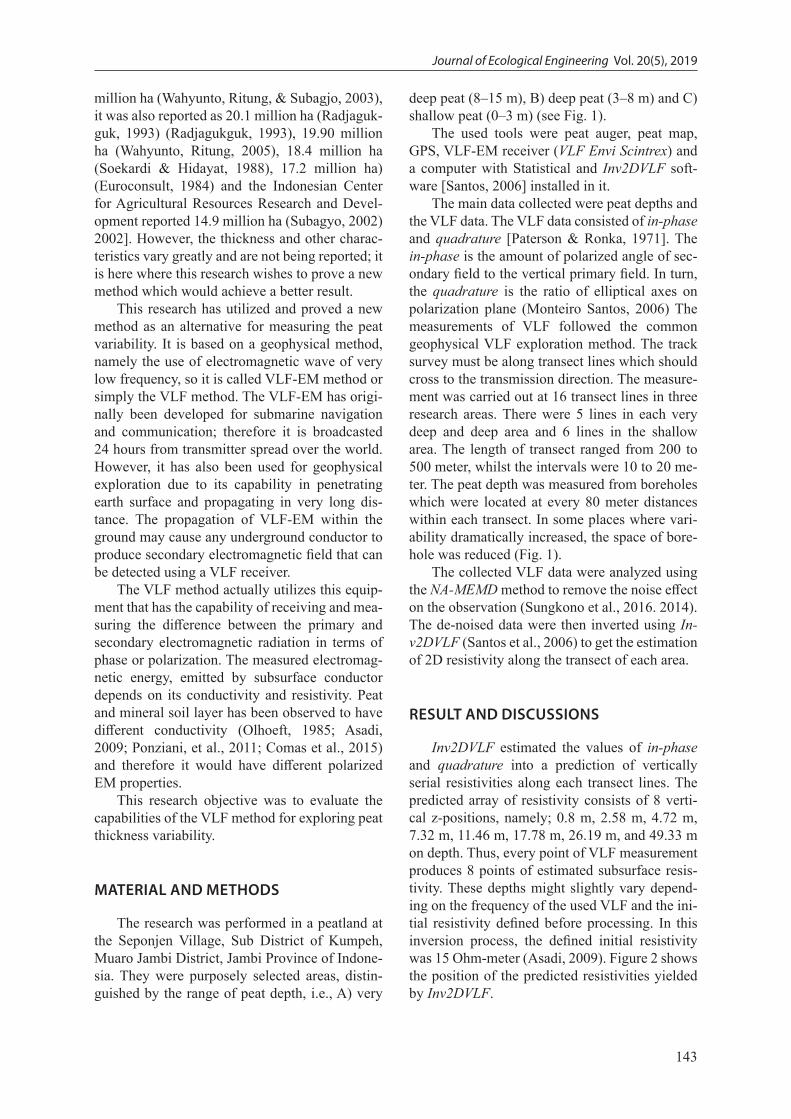
The research was performed in a peatland at the Seponjen Village, Sub District of Kumpeh, Muaro Jambi District, Jambi Province of Indone-sia. They were purposely selected areas, distin-guished by the range of peat depth, i.e., A) very

deep peat (8–15 m), B) deep peat (3–8 m) and C) shallow peat (0–3 m) (see Fig. 1).

The used tools were peat auger, peat map, GPS, VLF-EM receiver (VLF Envi Scintrex) and a computer with Statistical and Inv2DVLF soft-ware [Santos, 2006] installed in it.

The main data collected were peat depths and the VLF data. The VLF data consisted of in-phase and quadrature [Paterson & Ronka, 1971]. The in-phase is the amount of polarized angle of sec-ondary field to the vertical primary field. In turn, the quadrature is the ratio of elliptical axes on polarization plane (Monteiro Santos, 2006) The measurements of VLF followed the common geophysical VLF exploration method. The track survey must be along transect lines which should cross to the transmission direction. The measure-ment was carried out at 16 transect lines in three research areas. There were 5 lines in each very deep and deep area and 6 lines in the shallow area. The length of transect ranged from 200 to 500 meter, whilst the intervals were 10 to 20 me-ter. The peat depth was measured from boreholes which were located at every 80 meter distances within each transect. In some places where vari-ability dramatically increased, the space of bore-hole was reduced (Fig. 1).

The collected VLF data were analyzed using the NA-MEMD method to remove the noise effect on the observation (Sungkono et al., 2016. 2014). The de-noised data were then inverted using In-v2DVLF (Santos et al., 2006) to get the estimation of 2D resistivity along the transect of each area.

RESULT AND DISCUSSIONS

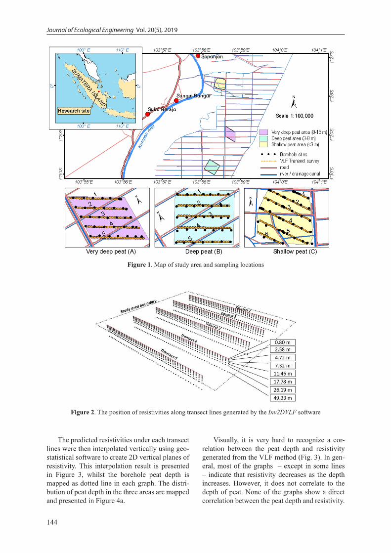
Inv2DVLF estimated the values of in-phase and quadrature into a prediction of vertically serial resistivities along each transect lines. The predicted array of resistivity consists of 8 verti-cal z-positions, namely; 0.8 m, 2.58 m, 4.72 m, 7.32 m, 11.46 m, 17.78 m, 26.19 m, and 49.33 m on depth. Thus, every point of VLF measurement produces 8 points of estimated subsurface resis-tivity. These depths might slightly vary depend-ing on the frequency of the used VLF and the ini-tial resistivity defined before processing. In this inversion process, the defined initial resistivity was 15 Ohm-meter (Asadi, 2009). Figure 2 shows the position of the predicted resistivities yielded by Inv2DVLF.


144

The predicted resistivities under each transect lines were then interpolated vertically using geo-statistical software to create 2D vertical planes of resistivity. This interpolation result is presented in Figure 3, whilst the borehole peat depth is mapped as dotted line in each graph. The distri-bution of peat depth in the three areas are mapped and presented in Figure 4a.

Visually, it is very hard to recognize a cor-relation between the peat depth and resistivity generated from the VLF method (Fig. 3). In gen-eral, most of the graphs – except in some lines – indicate that resistivity decreases as the depth increases. However, it does not correlate to the depth of peat. None of the graphs show a direct correlation between the peat depth and resistivity.

Figure 1. Map of study area and sampling locations

Figure 2. The position of resistivities along transect lines generated by the Inv2DVLF software

145


The variation of resistivity seems to exhibit dif-ferently among the 3 areas. In area A, the high resistivity (red color) is more concentrated in the upper layer, while in the other areas, they look sparser. Besides, there is a common pattern in most of graphs that the beginning of the lines is always high resistivity.

The statistical description and evaluation on the data of resistivity and peat depth would pro-duce better explanation. Table 1 shows the sta-tistics of resistivity and the next two tables de-scribe the result of mean comparison between and within the group based on the area from which it refers to and also based on its vertical depth.

In general, the average of resistivity tends to decrease as the depth increase. This can be seen from the data in Table 1. The line graph in Figure 4b shows the trend of decreased resistivity with the depth representing the three area and the average of overall data. The full lines show simi-lar trend of decreasing which can be represented by the logistic equation:

Area A: y = -4.849 ln(x) + 35.709 (R² = 0.8421) (1)

Area B: y = -6.305 ln(x) + 40.915(R² = 0.9453) (2)

Area C: y = -7.255 ln(x) + 43.428 (R² = 0.9318 (3)

Average: y = -6.136 ln(x) + 40.017 (R² = 0.919) (4)

where: y – denotes resistivity while, x – reprsents depth.

The graph indicates that the deeper from sur-face the lower the resistivity, meaning that the resistivity of the deep layer is lower than that of the shallow layer. This is related to the density of material, because the deep layer mostly con-sists of bedrock and compact material. The more compact the material, the easier the electrons pass through; thus, the higher the conductivity, the lower the resistivity (Seladji, et al., 2010)

When the mean of resistivity between group of peat depth (Table 2), as determined by one-way ANOVA (F[2.6317] = 4.525, p = 0.011) is com-pared, there is a statistically significant difference in resistivity. This difference, as revealed by the Tukey

Figure 3. Peat depth and vertical planes of resistivity from different transect lines and areas.


146

HSD test (Table 3), occurred between area A (very deep peat) and the area C (shallow peat). However, there were no difference between area A (very deep peat) and area B (deep peat), as well as between area C (shallow peat) and area B (deep peat).

The comparison between the three lines shows that the line representing very deep area (blue line) are the lowest among others, then followed by the line of deep area and the line of shallow area, respectively. This regular difference is more closely related to the water content or humidity and the soil pH. Peat thickness is comparable to its humidity and the acidity as well. The area of very deep peat holds more water than the shallow peat does; besides, it contains more contributor agent to acidity whilst the more water content, the lower resistivity (Asadi, 2009)

The most important finding is the result of comparison between the group of depth. When the resistivity is compared based on the group of depth (Table 4), there is also statistically sig-nificant difference in resistivity between group of depth (p = 0.000<0.05) in all areas. Furthermore,

these differences are revealed by the Tukey Test result (Table 5). This test result shows in de-tail how deep does the resistivity start to differ significantly. It shows that the resistivity of the upper layer tends to be statistically similar and starts to decrease with significant difference at the depth where peat disappears (boundary be-tween peat and mineral soil). The table shows that within the area A (very deep peat), resistiv-ity of 0.8 m, 2.58 m, 4.72 m and 7.32 m depth are considered to be not different statistically, but they are significantly different from those of 11.46 m, 17.78 m, 26.19 m and 49.33 m. In the area B (deep peat) the resistivity is consid-ered to be statistically similar from 0.8 m, 2.58 m and 4.72 m and is starts to be significantly different when the depth is 7.32 m or deeper.

The difference, as shown in the statistical test result, relates strongly with the characteris-tics of the area. The area A (very deep peat) has the range of peat from 8 to 15 meter. This is the boundary between peat and mineral soil. That is why, the average resistivity at lower 11.46 meter

Table 1. Predicted resistivity of inversion result

Depth Area A (very deep peat) Area B (deep peat) Area C (Shallow peat)

N Mean Std. dev N Mean Std. dev N Mean Std. dev0.8 m 245 33.72 50.92 245 39.94 49.56 300 41.98 48.98

2.58 m 245 33.97 44.41 245 37.49 43.56 300 40.26 41.884.72 m 245 30.75 33.95 245 32.82 33.44 300 35.28 32.577.32 m 245 26.01 22.11 245 28.60 23.10 300 28.01 22.2411.46 m 245 25.06 23.96 245 25.48 21.24 300 24.97 18.2217.78 m 245 21.57 18.42 245 22.93 22.75 300 21.92 16.2726.19 m 245 14.81 9.85 245 16.90 11.16 300 16.61 9.0949.33 m 245 18.58 6.57 245 17.58 6.81 300 16.89 5.43

Table 2. The ANOVA of mean comparison on the resistivity grouped by peat area.

Comparison Sum of Squares df Mean Square F Sig.Between Groups of peat area 8,387.879 2 4,193.939 4.525 .011Within Groups of peat area 5,854,862.479 6,317 926.842

Total 5,863,250.358 6,319

Table 3. The Tukey HSD of mean comparison on the resistivity grouped by peat area.

Between Mean Difference Std. Error Sig.95% Confidence

Lower Bound Upper Bound

Very deep (A):Deep (B) -2.15712 .97250 .068 -4.4369 .1227Shallow (C) -2.68211* .92686 .011 -4.8549 -.5093

Deep (B):Very deep (A) 2.15712 .97250 .068 -.1227 4.4369Shallow (C) -.52499 .92686 .838 -2.6978 1.6478

Shallow (C):Very deep (A) 2.68211* .92686 .011 .5093 4.8549Deep (B) 0.52499 .92686 .838 -1.6478 2.6978

Note: each value followed by star indicates significant differencea) The sparse of borehole peat depth, b) The trend of resistivity with the depth

147


is different from that of the upper. In turn, the peat depth of the area B (deep peat) ranges be-tween 3–8 meter, so the average resistivity tends to decrease and differ significantly at level of 7.32 meter. However, in area C (shallow peat), even though the decreasing of resistivity does not rich statistically significant, the difference of resistivity also happens at the depth of peat boundary. This can be seen from the graph (Fig 4b), the line representing the resistivity of the shallow area has the lowest gradient around 5 meter depth. These facts indicate that the resis-tivity measured from VLF fits the range of peat

depth. It means that the VLF resistivity corre-lates with the depth of peat.

The height of resistivity in upper layer (close to surface) in comparison to the depth of far from the surface is obvious. Peat is an organic material ac-cumulated in the upper mineral layer of soil and not completely weathered due to fully weathered con-dition over thousand years (Armanto et al., 2017). The abundance of organic material and water con-tent have made the peat porous and very light in density as well as much more homogeneous than mineral soil. Therefore, peat tends to exhibit lower electronic conductivity or higher resistivity.

Figure 4. Borehole peat depth and resistivity trend: a) The sparse of peat deph, b) The trend of resisivity with the depth

Table 5. Average resistivity by depth and The Tukey HSD result on each peat area

Depth Very deep peat Deep peat Shallow peat0.80 m 33.716 a 39.941 a 41.980 a

2.58 m 33.968 a 37.485 a 40.258 a

4.72 m 30.750 a 32.815 a 35.284 a

7.32 m 26.009 ab 28.595 b 28.014 b

11.46 m 25.062 bc 25.477 bc 24.967 b

17.78 m 21.571 c 22.934 c 21.919 bc

26.19 m 14.808 d 16.896 d 16.611 cd

49.33 m 18.583 d 17.581 d 16.891 cd

Note: each value in a column followed by different letter indicates significantly different at 0.05

Table 4. The ANOVA of mean comparison on resistivity grouped by depth on each peat area

Peat Area Comparison Sum of Squares df Mean Square F Sig.

Very deep area

Between Groups of depth 84,481.246 7 12,068.749 13.298 .000Within Groups of depth 1,771,570.472 1,952 907.567Total 1,856,051.718 1,959

Deep areaBetween Groups of depth 127,238.226 7 18,176.889 20.352 .000Within Groups of depth 1,743,355.210 1,952 893.112Total 1,870,593.437 1,959

Shallow areaBetween Groups of depth 160,056.167 7 22,865.167 23.732 .000Within Groups of depth 1,880,673.300 1,952 963.460Total 2,040,729.467 1,959

a) b)


148

CONCLUSIONS

The following conclusions can be drawn from the research:1. VLF method is applicable in peat area and

shows the variability of peat resistivity.2. VLF based resistivity tends to decrease as the

depth increases.3. The average resistivity of the thicker peat area

is significantly lower than the thinner peat area.4. The vertical resistivity of peat in the area of

very deep peat (8–15 m) and deep peat (3–8 m) tends to remain unchanged statistically till the depth where peat changes to mineral soil (peat depth boundary).

Acknowledgements

Our gratitude and appreciation go to the proj-ect leader of CRC990, Stefan Scheu for funding this research and to Christoph Kleinn (the Princi-pal Investigator of B05 sub-project in CRC990) and Lutz Fehrmann (CRC researcher) for the great help given to carry out the research.

REFERENCES

1. Agus, F. and Subiksa, I.G.M. 2008. Lahan Gam-but : Potensi untuk Pertanian dan Aspek Lingkun-gan. Balai Penelitian Tanah, Badan Penelitian dan Pengembangan Pertanian. Bogor. Retrieved from http://www.worldagroforestry.org/sea/publica-tions/files/book/BK0135–09.PDF

2. Armanto, M.E. 2002. Mapping Construction of Soil Variability Within The Landscape. Jurnal Bi-onatura, 4(3), 189–197.

3. Armanto, M.E. 2014. Spatial Mapping for Man-aging Oxidized Pyrite (FeS2) in South Sumatra Wetlands , Indonesia. Journal of Wetlands Envi-ronmental Management, 2(2), 60–66.

4. Armanto, M.E., Wildayana, E., Imanudin, M.S., Junedi, H., Zuhdi, M. 2017. Selected Properties of Peat Degradation on Different Land Uses and the Sustainable Management. Journal of Wetlands Environmental Management, 5(2), 14. https://doi.org/10.20527/jwem.v5i2.120

5. Asadi, A. and Huat, B.B.K. 2009. Electrical Resis-tivity of Tropical Peat. Electronic Journal of Geo-technical Engineering, 14P, 1–9.

6. Comas, X., Terry, N., Slater, L., Warren, M., Kol-ka, R., Kristiyono, A., et al. 2015. Imaging tropical peatlands in Indonesia using ground-penetrating ra-dar (GPR) and electrical resistivity imaging (ERI):

implications for carbon stock estimates and peat soil characterization. Biogeosciences, 12(10), 2995–3007. https://doi.org/10.5194/bg-12–2995–2015

7. Euroconsult. 1984. Final report of preliminary as-sessment of peat development potential. Co-opera-tive between Kingdom of Netherland and Ministry of Foreign Affairs Indonesia. Jakarta.

8. Limin, S.H. 2006. Pemanfaatan Lahan Gambut dan Permasalahannya. Workshop Gambut : Peman-faatan Lahan Gambut Untuk Pertanian, Jakarta.

9. Monteiro Santos, F. A. 2006. Inv2DVLF. Centro de Geofísica da Universidade de Lisboa.

10. Olhoeft, G.R. 1985. Low-frequency electrical prop-erties. Geophysics, 50(12), 2492–2503. https://doi.org/10.1190/1.1441880

11. Paterson, N.R. and Ronka, V. 1971. Five years of surveying with the Very Low Frequency-Electro magnetics method. Geoexploration, 9(1), 7–26. https://doi.org/10.1016/0016–7142(71)90085–8

12. Ponziani, M., Slob, E.C., Vanhala, H. 2011. In-fluence of Water Content on The Electrical Con-ductivity of Peat. International Water Technology Journal, I(1), 14–21.

13. Radjagukguk, B. 1993. Peat resources of Indo-nesia: its extern, characteristics and development possible. In The Third Seminar on the Greening of Desert entitled “Desert Greening with Peat”. Wese-da University (p. 1993). Tokyo.

14. Seladji, S., Cosenza, P., Tabbagh, A., Ranger, J., Richard, G. 2010. The effect of compaction on soil electrical resistivity : a laboratory investigation, (December), 1043–1055. https://doi.org/10.1111/j.1365–2389.2010.01309.x

15. Soekardi, M. and Hidayat, A. 1988. Extern and dis-tribution of peat soils of Indonesia. In The Third Meeting of the Cooperative for Research on Soil Problems (p. 1988). Bogor.

16. Subagyo, H. 2002. Penyebaran dan Potensi Gam-but di Indonesia untuk Pembangunan Pertanian. Prosiding Lokakarya Kajian Status Dan Sebaran Gambut Di Indonesia, 197–222.

17. Sungkono, Santosa, B.J., Bahri, A.S., Santos, F.M., Iswahyudi, A. 2016. Application of Noise-Assist-ed Multivariate Empirical Mode Decomposition in VLF-EM Data to Identify Underground River. Advances in Data Science and Adaptive Analy-sis, 8(October), 1–23. https://doi.org/10.1142/S2424922X1650011X

18. Wahyunto, Ritung, S. 2005. Sebaran Gambut dan kandungan Karbon di Sumatra dan Kalimantan. Bo-gor: Wetlands International-Indonesia Programme.

19. Wahyunto, Ritung, S. and Subagjo, H. 2003. Peta Luas Sebaran Lahan Gambut dan Kandungan Karbon di Pulau Sumatera / Map of Area of Peatland Distri-bution and Carbon Content in Sumatera, 1990–2002.

Documents

Exploring Peat Thickness Variability Using VLF Method Peat Thickness.pdf · In turn, in the area of deep peat, it is statistically similar until 4.72 meter and starts to show differences