Seediscussions,stats,andauthorprofilesforthispublicationat:https://www.researchgate.net/publication/268447000

Explorationofelectricityusagedatafromsmartmeterstoinvestigatehouseholdcomposition

ConferencePaper·September2013

CITATION

1

READS

9

4authors,including:

PaulaCarroll

UniversityCollegeDublin

15PUBLICATIONS14CITATIONS

SEEPROFILE

Availablefrom:PaulaCarroll

Retrievedon:15September2016

1

Distr. GENERAL

13 September 2013 WP 29

ENGLISH ONLY

UNITED NATIONS ECONOMIC COMMISSION FOR EUROPE CONFERENCE OF EUROPEAN STATISTICIANS

Seminar on Statistical Data Collection (Geneva, Switzerland, 25-27 September 2013) Topic (v): Integration and management of new data sources EXPLORATION OF ELECTRICITY USAGE DATA FROM SMART METERS TO INVESTIGATE HOUSEHOLD COMPOSITION Working Paper Prepared by Paula Carroll (University College Dublin, UCD) , John Dunne (Central Statistics Office, Ireland) , Michael Hanley (UCD) , Tadhg Murphy (UCD)

I. Introduction

1. In the digital world of today, new sources of data are being identified that have the potential to make a significant contribution to the production of official statistics. Some of these data sources (sometimes referred to as “Big data”) will require new techniques and skills to extract the underlying value. In this paper we describe a case study investigating how one such data source might be integrated with official statics production. We outline the data mining technique used and some of the challenges encountered.

2. The Commission for Energy Regulation (CER) is the regulator for the electricity and gas sectors in Ireland. Historically, electricity usage has been measured by electromechanical meters. A smart metering system combines an electronic meter (often with a display unit for consumers to use in the home) with a communication layer for sending data to and from the supplier. The CER initiated a Smart Metering Project in 2007 with the purpose of undertaking trials to assess the performance of Smart Meters and their impact on consumer behaviour. Customer Behaviour Trials (CBTs) took place during 2009 and 2010. The Smart Meter Data (SMD) were made available to facilitate further research1.

3. This offered the opportunity for the data to be queried to answer questions other than those for which the data were originally gathered. The Central Statistics Office (CSO) of Ireland in collaboration with a team from University College Dublin (UCD) sought to identify:

(a) What insight SMD can provide about household composition,

(b) The challenges and opportunities in exploring and harnessing the benefits of SMD.

1 http://www.ucd.ie/issda/data/commissionforenergyregulationcer/

2

II. Smart Meter Data

A. Challenges

4. The CBT ran for a six month benchmark period and a one year test period with 5,375 “opt-in” participants. Half-hourly electricity usage was recorded during the benchmark and test periods for each household. During the test period, different ToU (time of use) tariff structures were used to see how they modified customer behaviour. A pre-trial survey was conducted using a computer-assisted telephone interview (CATI) system and included a range of questions about household demographics and the home itself. The data were gathered to assess the impact on behaviour, not to answer questions posed by the CSO.

5. Over 150 Million records of usage alone are included in the SMD, approximately 2.5 G of data in total were made available in multiple files. Standard workplace laptops or desktops struggle to process such volumes of data. The options when working with such volumes of data are to aggregate, to sample, to apply data reduction techniques and/or to use additional hardware.

6. The SMD is well structured and well documented. It contains a unique meter identifier for each household. This allows the benchmark and test period usage to be linked with each household and their pre-trial survey responses. However, other open source or third part data may not be as structured.

7. The question of data integrity arises in dealing with third-part data. Decisions must be made on how to handle outliers, missing values and incomplete records.

8. In addition the data may be unbalanced with an over representation of some categories. Consider for example a familial category which corresponds to 90% of the participants, only 10% of the data corresponds to other household categories. A simple guessing strategy would correctly identify households 90% of the time but the objective is to achieve a fairly high rate of correct detection in the minority class. Undersampling techniques may be used to re-balance the class distribution.

9. An appropriate algorithmic technique must be selected to answer the question of interest. Machine learning is the process of a computer code adapting its behaviour (the accuracy of the output it produces) in response to some input data. In this instance we want an algorithm that classifies household composition according to electricity usage. Classification is a method that describes data with discrete or categorical labels. (Artificial) Neural Networks ((A)NNs) are machine learning algorithms suited to such a classification task.

10. Finally, we note that issues of data privacy arise in relation to exploring the SMD. The data used in this project is made available as an anonymised micro data file under provisions laid down in Statistics Act, 19932. The intended use of the Anonymised microdata file is for teaching and research purposes.

B. Opportunities

11. The availability of data sets such as SMD offer possible cost savings to state organisations. Knowledge of household composition or other household characteristics could contribute to the development of an alternative Census model or provide insight into a changing population in the intervening years. Such knowledge could assist in areas such as local government planning, for example knowing that a household contains children. In particular electricity usage might indicate when members of the household are likely to be at home which would assist in the scheduling calls by field staff – however consideration needs to be given to proportionality in terms of the use at a household level.

2 http://www.irishstatutebook.ie/1993/en/act/pub/0021/print.html

3

12. Administrative data received from public bodies may be combined with additional data sources such as SMD to allow a more complete picture of typical lifestyles and patterns to be built so as to inform decision and policy making.

13. In exploring third part and open source data to answer a specific question, subject area experts may spot patterns or unusual trends. In identifying or explaining these patterns, we may find the answer to questions other than those originally asked.

III. Road map to extracting insight from “Big Data”

14. Data Mining techniques are used to explore and extract useful insights, particularly from “Big Data”. Machine Learning algorithms can be used to classify input vectors of length m into one of K classes. This involves a two-step procedure of learning and testing. In the first step, the class labels must be learned from a training set of data followed by a testing or validation step where the model is tested for accuracy. Perhaps the most important concept in machine learning is that of generalisation, that is, the algorithm should produce sensible outputs for inputs that were not encountered during learning3.

15. Each input vector component is associated with an important attribute of the data. Selecting a minimal set of appropriate vector components is a challenging task requiring statistical analysis of the data. If too many or un-influential components are used, the algorithm run-time and solution quality can be negatively affected. We wish to identify a small number of explanatory variables (or features) that best represent the full data set.

16. Dimension Reduction (DR) involves the conversion of data with high dimension into data of much lower dimension to obtain a reduced or compressed representation of the original data. The reduced set is used as the inputs to the NN.

17. Statisticians sometimes talk of problems that are “Big p Small n"; these are extreme examples of situations where DR is necessary because the number of explanatory variables p exceeds (sometimes greatly exceeds) the number of samples n. Machine Learning algorithms are susceptible to the “curse of dimensionality”, which refers to the degradation in the performance of a given learning algorithm as the number of features increases. DR approaches focus on either selecting a subset of the existing features or on transforming to a new reduced set of features.

18. Principal Component Analysis (PCA) is a transformational method of DR that seeks to find a lower dimensional set of axes that best describe the data and can be used to identify the most representative features as inputs to a classifier4. The transformed features may have no physical meaning to the domain expert.

19. A number of studies have investigated the variables that influence domestic energy consumption. The algorithmic techniques used and sets of influential variables selected depend on the questions the authors are trying to answer. The top 4 variables in general are: dwelling type, income, household appliances and number of occupants5. Other relevant work in this area is summarised in 6, 7 and 8.

3 Marsland, S., 2009. Machine learning: an algorithmic perspective, Chapman & Hall/CRC. 4 Malhi, A. & Gao, R.X., 2004. PCA-Based Feature Selection Scheme for Machine Defect Classification. IEEE Transactions on

Instrumentation and Measurement, 53(6), pp.1517–1525. 5 McLoughlin, F., Duffy, A. & Conlon, M., 2012. Characterising domestic electricity consumption patterns by dwelling and

occupant socio-economic variables: An Irish case study. Energy and Buildings, 48(July 2009), pp.240–248. 6 Yohanis, Y.G. et al., 2008. Real-life energy use in the UK: How occupancy and dwelling characteristics affect domestic

electricity use. Energy and Buildings, 40(6), pp.1053–1059. 7 O’Doherty, J., Lyons, S. & Tol, R.S.J., 2008. Energy-using appliances and energy-saving features: Determinants of ownership

in Ireland. Applied Energy, 85(7), pp.650–662. 8 Druckman, a & Jackson, T., 2008. Household energy consumption in the UK: A highly geographically and socio-economically

disaggregated model. Energy Policy, 36(8), pp.3177–3192.

4

20. The type of learning where an input is matched to a known output is termed supervised learning and forms the basis of NNs. NNs derive from an analogy with how the brain works9. NN nodes (analogous to neurons in the brain) form a connected network capable of modelling or “learning” some data. NNs are weighted directed graphs where each node is connected only to nodes in layers other than its own, a visualisation is shown below.

Figure 1: The McCulloch Pitts model of an artificial neuron

21. NNs can be characterised by four main features. The connection topology describes how the nodes are connected to each other. Basis functions define the processing carried out by each node on its weighted combination of inputs. The training method determines how the NN learns, as well as the supervised approach described above, unsupervised learning can be used to identify patterns in the data. Lastly, the learning/training algorithm controls how the NN reduces error throughout the training process.

22. A Multi Layer Perceptron (MLP) is a type of NN which uses an error back-propagation algorithm to train the network. During a forward pass, an input vector propagates through the entire network, producing a set of outputs and edge weights are estimated. The error is calculated as the difference between the output from the forward pass and the actual known output of the training dataset. On a backward pass, the weights are adjusted according to some error-correction rule (for example, gradient descent function) to produce an error signal. This is then fed back across the network. This error signal causes the edge weights to be adjusted so that the network response is moved closer to the desired output.

IV. Case Study Approach Used

C. Hardware and Software Decisions

23. Several layers of data pre-processing and data reduction as well as feature extraction and signal processing were used to produce useful inputs for the neural network. The software selection criteria were that the package used to process the high volumes of CER data be readily or freely available, easy to use and be capable of carrying out the classification task.

24. Desktop packages were not suitable due to the data size. While standard statistical packages may be more suited to statistical tasks, costly licenses maybe required. Open source environments can lead to easier sharing of solution approaches. Given the limited time frame of this project, we selected R10 to perform both the data manipulation and analysis due to its open source nature. R provides a wide range of statistical techniques such as linear and non-linear modelling, classical statistical tests, time series analysis, classification, clustering and data visualisation tools.

25. The base R system comes with 8 packages with additional packages being made available through the Comprehensive R Archive Network (CRAN)11. Additional packages are available to create and

9 Gurney, K., 1997. An Introduction to Neural Networks, Taylor & Francis, Inc. 10 http://www.r-project.org 11 http://CRAN.R-project.org

5

analyse NNs. Four neural network packages were investigated initially to determine which was the most appropriate for use in this project. These packages were nnet, neuralnet, AMORE and RSNNS. The nnet and neuralnet packages were found to be in more widespread use and were easier to implement so were selected for the task of creating and analysing NNs.

26. The next consideration was whether standard laptops or desktops could be used. Initial exploratory data analysis tasks on a high spec laptop (Acer, Windows 8, 3.2GHz Intel i7 processor, 8 G RAM) required over 12 hours to manipulate the raw data files into a suitable format. As this was not practical the Stokes supercomputer at the Irish Centre for High-end Computing (ICHEC)12 was used.

27. Stokes was funded under a Programme for Research in Third Level Institutions. Access to ICHEC systems is available free of charge to members of the Irish 3rd level research community subject to an application process. The Lynux-based Stokes supercomputer has 320 compute nodes each with 12 cores and 2 GB of RAM per core. Each compute node has two Intel (Westmere) Xeon E5650 hex-core processors and 24GB of RAM. In total, 3840 cores and 7680GB of RAM available.

28. Connection to the Stokes system was achieved using the Secure Shell protocol (SSH) and is only possible over a contributing institution IP address. An open source, terminal emulator and serial console called PuTTY was used to connect the MS Windows based laptop to Stokes. Jobs were submitted to Stokes using a batch queuing process by submitting a script detailing the resources required and the command required to run the job.

D. Data Preparation

29. The pre-trial survey consisted of 140 questions. These data were used to extract the known composition of each household, that is, the number of members in each household. However, a limiting factor is that detailed information is only given for the Head of Household. The only distinction between adults and children is that the number of children under 15 years of age is given.

30. In addition, the number of households consisting of two adults and no children (1,264) far exceeded any other family type. The problem of unbalanced data, where the proportions of data in the K classes are not similar, is significant in the field of machine learning and may lead to mis-classification. The number of participants and classes are shown below.

Figure 2: House hold Composition 12 ICHEC is Ireland’s national high performance computer centre

Categories A B C D E F G H I J K L M N O PAdults 3 3 3 2 2 2 2 2 2 1 1 4 4 5 5 6Children 2 1 0 5 4 3 2 1 0 1 0 1 0 1 0 0

6

31. The R Studio package was used to merge the multiple usage files to create a single dataframe. This is an integrated development environment for R with a Graphical User Interface. Records for meters with missing half-hour readings, incomplete questionnaire data or invalid time stamps were removed from the data set. This left 4,174 complete record sets for analysis. Data of this size can reasonably be handled without the need for sampling on the Stokes machine. However, in other instances the data would be too large and would need to be sampled.

32. The remaining data were aggregated across the half-hour time slots using samples varying in size from 24 hours to 6 months. Individual data within the meters was not subjected to any outlier analysis, instead this was performed on the aggregated data for each meter. This approach ensured that potentially useful data within individual meters was not removed however any outlying households were removed before the data was input to the classifier. This method was deemed the most suitable for preserving the integrity of the data set and removing a possible source of error from the classification process. Density-based local outlier detection was chosen for the task of outlier detection, specifically the local outlier factor (LOF) algorithm13.

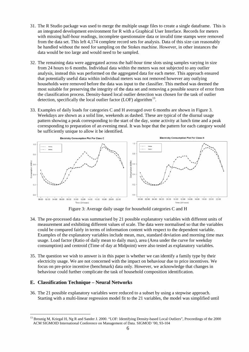
33. Examples of daily loads for categories C and H averaged over 6 months are shown in Figure 3. Weekdays are shown as a solid line, weekends as dashed. These are typical of the diurnal usage pattern showing a peak corresponding to the start of the day, some activity at lunch time and a peak corresponding to preparation of an evening meal. It was hope that the pattern for each category would be sufficiently unique to allow it be identified.

Figure 3: Average daily usage for household categories C and H

34. The pre-processed data was summarised by 21 possible explanatory variables with different units of measurement and exhibiting different values of scale. The data were normalised so that the variables could be compared fairly in terms of information content with respect to the dependent variable. Examples of the explanatory variables include mean, max, standard deviation and morning time max usage. Load factor (Ratio of daily mean to daily max), area (Area under the curve for weekday consumption) and centroid (Time of day at Midpoint) were also tested as explanatory variables.

35. The question we wish to answer is in this paper is whether we can identify a family type by their electricity usage. We are not concerned with the impact on behaviour due to price incentives. We focus on pre-price incentive (benchmark) data only. However, we acknowledge that changes in behaviour could further complicate the task of household composition identification.

E. Classification Technique – Neural Networks

36. The 21 possible explanatory variables were reduced to a subset by using a stepwise approach. Starting with a multi-linear regression model fit to the 21 variables, the model was simplified until

13 Breunig M, Kriegal H, Ng R and Sander J. 2000. “LOF: Identifying Density-based Local Outliers”, Proceedings of the 2000

ACM SIGMOID International Conference on Management of Data. SIGMOD ’00, 93-104

7

only the most statistically significant (p < 0.1) variables remained. The remaining reduced set were selected as the inputs to the NN.

37. Two NN approaches were tested. The first approach involved a binomial classifier whereby a binary question is asked. We wished to determine whether a particular meter belonged to a particular household category. The output from the NN was a value in the range [0,1] indicating the probability of the meter belonging to that household category.

38. The disadvantage of this approach was that the model had to be run separately for each household category and so involved extra data manipulation and significantly more coding.

39. The second approach involved a multinomial classifier where a question involving multiple possible answers was posed to the classifier. We wished to determine to which household category a meter most likely belonged. The NN output is a vector of K components corresponding to the K classes. Each component has a value in the range [0,1] indicating the probability that the meter belongs to the Kth class. The sum of the component values is 1.

40. The advantage of the second NN approach was that only one model was run and so less manipulation of the data was required, however, as the classifier was presented with more options to choose from it could potentially lead to a significant reduction in accuracy.

41. The data were divided into three subsets for training, testing and validation of the network. The training set was used to calculate the NN weights and bias inputs which minimise the error in the network. The validation set was used to ensure that no over-fitting of the training data occurred. Finally, the test set was used to verify the classifier accuracy. The breakdown chosen for the data into a three way split was selected as 60-20-20 (training-testing-validation) of the reduced data set.

42. The training data sample was drawn by random selection without replacement. Half of the remaining data were drawn by random selection without replacement to form the validation set, the remaining data formed the test set.

43. The error measurement used for the binomial NN was the root mean-squared error (RMSE). This measure is calculated by taking the square root of the average squared differences difference between the actual and predicted values of each meter. The error was computed at each iteration of the NN training. When the RMSE error using the validation set registered two consecutive increases the training of the network was stopped. This flagged the point at which the training algorithm has started to over-fit the data. This NN model was then applied to the test set to determine its predictive ability. Separate binomial NNs were created for each of the household categories.

44. A multinomial NN model was developed using a similar approach but using the Sum of Cross Entropy (SCE) as the error measure. The cross entropy error is computed by determining the negative sum of the product of the actual value and the log of the predicted value of the dependent variable. It is computed for each of the meters in the dataset and is summed over the entire dataset to get the sum of cross entropy error for the dataset.

45. Confusion matrices were used to visualise of the performance of the NN classifier. It indicates the number of false positives, false negatives, true positives, and true negatives.

46. We also investigated the performance of the two NN models by selecting the training data using undersampling techniques. That is, for the binomial NN, balanced datasets were created for the household categories containing the records in that category (flagged as True) and an equal number of records from families not in that category which were selected at random.

47. An undersampling technique was tailored to suit the multinomial classifier. A threshold was used to select categories with more than 105 participants. Categories with smaller numbers of participants, such as category D containing only 9, were deemed too small for any statistical analysis. These

8

categories were not considered for testing by the multinomial model. The sample size for each remaining category was restricted to 210 split evenly between True/False.

V. Results and Key Points

F. Summary Statistics

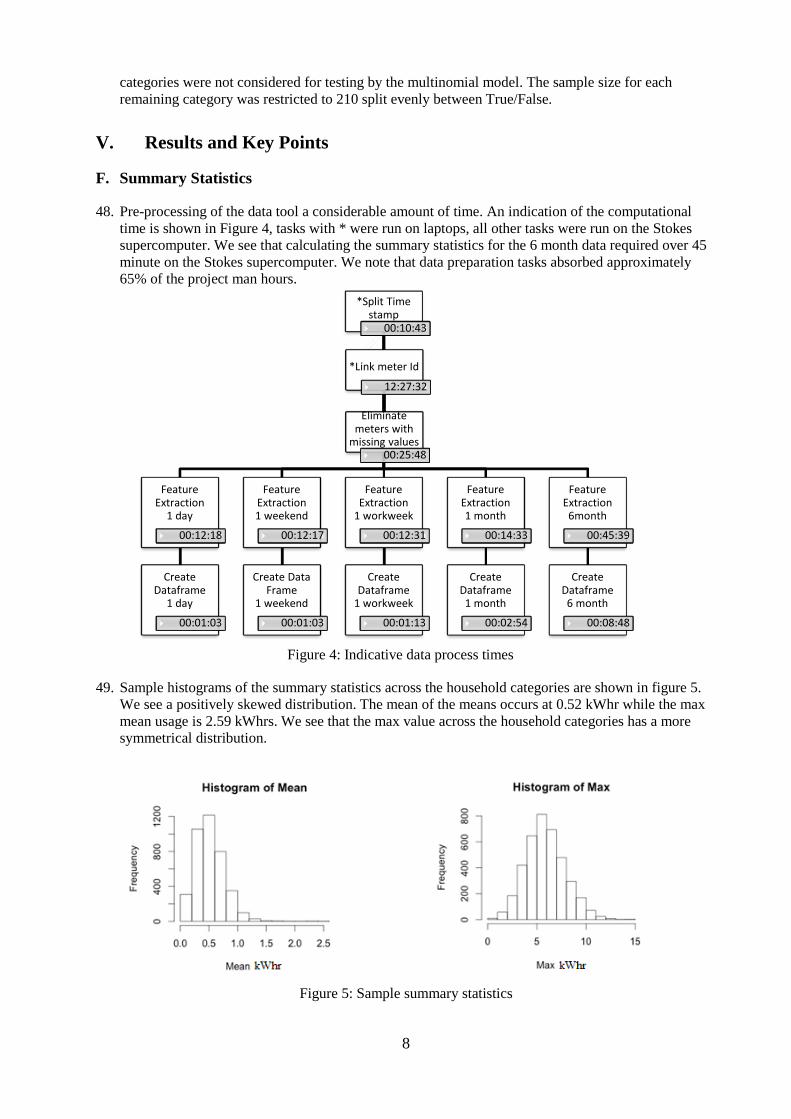
48. Pre-processing of the data tool a considerable amount of time. An indication of the computational time is shown in Figure 4, tasks with * were run on laptops, all other tasks were run on the Stokes supercomputer. We see that calculating the summary statistics for the 6 month data required over 45 minute on the Stokes supercomputer. We note that data preparation tasks absorbed approximately 65% of the project man hours.

Figure 4: Indicative data process times

49. Sample histograms of the summary statistics across the household categories are shown in figure 5. We see a positively skewed distribution. The mean of the means occurs at 0.52 kWhr while the max mean usage is 2.59 kWhrs. We see that the max value across the household categories has a more symmetrical distribution.

Figure 5: Sample summary statistics

*Split Time stamp

00:10:43

Feature Extraction

1 day 00:12:18

Create Dataframe

1 day 00:01:03

Feature Extraction 1 weekend

00:12:17

Create Data Frame

1 weekend 00:01:03

Feature Extraction

1 workweek 00:12:31

Create Dataframe

1 workweek 00:01:13

Feature Extraction 1 month

00:14:33

Create Dataframe 1 month

00:02:54

Feature Extraction

6month 00:45:39

Create Dataframe 6 month

00:08:48

*Link meter Id

12:27:32

Eliminate meters with

missing values 00:25:48

9

50. A box plot of the mean daily usage, Figure 6, highlights the increasing trend in mean values as the number of occupants within the house increases. We would expect that this increase in mean consumption would allow the NN classifier to better distinguish between household categories.

Figure 6: Boxplot of mean daily usage per household category

G. Classifier Results

51. A multiple linear regression (MLR) model was created for comparison purposes. The best fit MLR model incorporated the mean, load factor, variance, standard deviation, area and centroid statistics as explanatory variables. The value of R2 for this model was 0.04 indicating that it is not a good fit for the data. An F-test confirmed the unsuitability of the MLR model.

52. Initial PCA analysis identified 4 components but this gave limited scope to identify the 16 household categories so this avenue was not pursued.

53. The best binomial NN was obtained using balanced data and had an R2 value of 0.54. A sample confusion matrix is shown for household category G. more households are classified as “false” than “true” and if we look at the confusion matrix we see that 224 meters are classified as “false” and 172 meters classified as “true”. The classifier is therefore giving “false negatives”.

54. Scatter plots are useful to visualise the partitioning ability of the classifier. The y-axis refers to predicted probability (equivalent to the probability that meter belongs to a particular class). The number of distinct predicted probability output values will equal the no. of classes in the classifier. The x-axis labelled as index refers to the ith object in the dataset.

Test Predicted

False True Σ

Actu

al False 48 18 66

True 29 37 66 Σ 77 55 132

Figure 7a: Sample confusion matrix for household category G with a binomial NN using balanced data

Figure 7b: Prediction scatter plot for household category K with a binomial NN using balanced data

10

55. We see in Figure 7b that data are evenly distributed data between the upper and lower halves of the plot area. The majority of the predictions are concentrated in the top and bottom quarters of the plot area as expected from a good classifier. These plots show that the classifier has similar prediction accuracy in both the “yes” and “no” class.

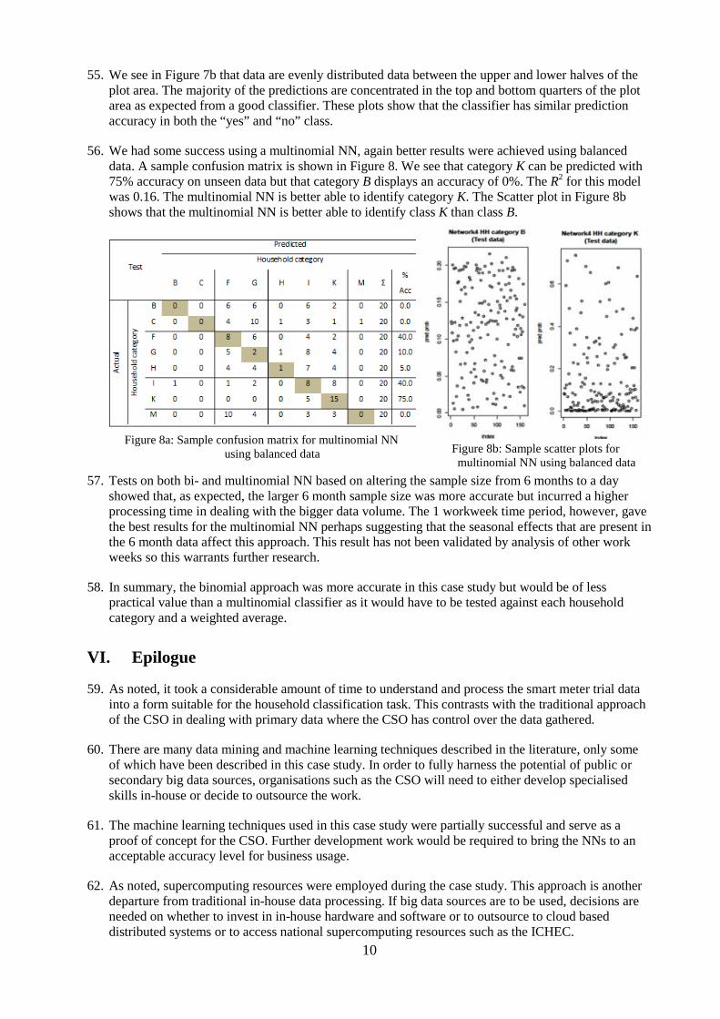
56. We had some success using a multinomial NN, again better results were achieved using balanced data. A sample confusion matrix is shown in Figure 8. We see that category K can be predicted with 75% accuracy on unseen data but that category B displays an accuracy of 0%. The R2 for this model was 0.16. The multinomial NN is better able to identify category K. The Scatter plot in Figure 8b shows that the multinomial NN is better able to identify class K than class B.

57. Tests on both bi- and multinomial NN based on altering the sample size from 6 months to a day showed that, as expected, the larger 6 month sample size was more accurate but incurred a higher processing time in dealing with the bigger data volume. The 1 workweek time period, however, gave the best results for the multinomial NN perhaps suggesting that the seasonal effects that are present in the 6 month data affect this approach. This result has not been validated by analysis of other work weeks so this warrants further research.

58. In summary, the binomial approach was more accurate in this case study but would be of less practical value than a multinomial classifier as it would have to be tested against each household category and a weighted average.

VI. Epilogue

59. As noted, it took a considerable amount of time to understand and process the smart meter trial data into a form suitable for the household classification task. This contrasts with the traditional approach of the CSO in dealing with primary data where the CSO has control over the data gathered.

60. There are many data mining and machine learning techniques described in the literature, only some of which have been described in this case study. In order to fully harness the potential of public or secondary big data sources, organisations such as the CSO will need to either develop specialised skills in-house or decide to outsource the work.

61. The machine learning techniques used in this case study were partially successful and serve as a proof of concept for the CSO. Further development work would be required to bring the NNs to an acceptable accuracy level for business usage.

62. As noted, supercomputing resources were employed during the case study. This approach is another departure from traditional in-house data processing. If big data sources are to be used, decisions are needed on whether to invest in in-house hardware and software or to outsource to cloud based distributed systems or to access national supercomputing resources such as the ICHEC.

Figure 8a: Sample confusion matrix for multinomial NN

using balanced data Figure 8b: Sample scatter plots for multinomial NN using balanced data

11

63. All outsourcing options give rise to new data protection and security issues which were not given consideration within the scope of this case study.