Minerals Engineering 25 (2012) 20–27

Contents lists available at SciVerse ScienceDirect

Minerals Engineering

journal homepage: www.elsevier .com/ locate/mineng

Experimental validation of 2D DEM code by digital image analysis in tumbling mills

C. Pérez-Alonso, J.A. Delgadillo ⇑Facultad de Ingeniería – Instituto de Metalurgia, Universidad Autónoma de San Luis, Av. Sierra Leona #550, Lomas 2da Sección, San Luis Potosí, SLP 78210, Mexico

a r t i c l e i n f o a b s t r a c t

Article history:Received 8 March 2011Accepted 30 September 2011Available online 28 October 2011

Keywords:Tumbling millsDEMDigital image analysisVelocity profileMineral processing

0892-6875/$ - see front matter � 2011 Elsevier Ltd. Adoi:10.1016/j.mineng.2011.09.018

⇑ Corresponding author.E-mail address: jose.delgadillo@uaslp.mx (J.A. Delg

The discrete element method (DEM) is widely used as an optimization tool in the design of tumblingmills. Nevertheless, the experimental validation of DEM codes is an important step to guarantee thatthe system is well described and that the predictions are close to the real operating conditions. The powerdraw is the principal parameter used to validate DEM codes, but using this as the only reference can beinappropriate. The power draw can be fitted by simply changing the model constants until the predictedvalues are close to the experimental data, when the charge profile looks similar to the real operation andthere is no experimental velocity profile with which to compare. This paper presents an experimental val-idation of a 2D DEM code by digital image analysis of the velocity profiles of the balls, the toe and shoul-der angles and the predicted power draw. The experimental values were compared with the simulateddata using different charge lifters and charge levels. The DEM simulation clearly shows that the velocitycharge changes with a modification of the lifter profile. An accurate map of velocities at each location inthe mill was obtained by digital image analysis and compared with DEM calculations. The simulated andexperimental values are very close, leading to the conclusion that such DEM predictions represent anaccurate description of the process in a tumbling mill.

� 2011 Elsevier Ltd. All rights reserved.

1. Introduction

The size reduction process is one of the most important pro-cesses in raw material transformation. In the mineral processingarea, particle size reduction is accomplished primarily by ball mills.For instance, in the cement industry, grinding is the key processdetermining the quality of the final product. Between 60% and90% of the total cement production cost is due to energy consump-tion (Austin et al., 1984). Therefore, the grinding process must beoptimized to minimize grinding costs.

Usually, the optimization and design of grinding circuits arebased on costly and time- consuming laboratory experimentationand pilot plant testing. Additionally, the velocity and energy im-pacts inside the mills are very different between the laboratoryscale and an industrial mill. The scale-up process modifies the frac-ture behavior of the particles (Datta and Rajamani, 2002). The solu-tion to this problem is the use of numerical tools, such as thediscrete element method (DEM), that can predict the behavior ofgranular materials. The DEM is a novel technique to optimizeand design mills with minimal experimental effort, and it can beeasily scaled up from the laboratory to an industrial size mill. Overthe past decade, many researchers have proposed the use of DEMto predict the charge profile in tumbling mills, but most have fo-cused on the charge profile to validate codes (Cleary, 1998, 2000,

ll rights reserved.

adillo).

2001a,b, 2009; Inoue and Okaya, 1995, 1996; Kano et al., 1997;Mishra, 1991; Mishra and Rajamani, 1990, 1992, 1994a,b; Rajama-ni and Mishra, 1996; Rajamani et al., 1999, 2000; Powell and Nur-ick, 1996; Radziszewski, 1999; Zhang and Whiten, 1996, 1998;Buchholtz et al., 2000; Cleary and Hoyer, 2000; Nierop van et al.,2001; Cleary et al., 2003).

Nevertheless, experimental validation is the most importantstep in the process of testing codes. The most frequently used val-idation methodologies are ball trajectory tracking and power drawmonitoring in laboratory scale mills (Venugopal and Rajamani,2001; Dong and Moys, 2002; Mishra and Rajamani, 1994a). Thetrajectory of the balls can be tracked by digital image analysis(DIA). The velocity can be calculated using DIA, as this techniquehas been shown to be able to generate the particle path lines usingfluorescence microscopy (Meijering et al., 2004). The code used inthis paper was developed in the laboratory of mineral processingsimulation at the Autonomous University of San Luis Potosi(UASLP) and is described as follows.

The code is written for a two-dimensional system with interac-tion forces between the particles of a granular material. This sys-tem is represented by spherical particles that are in mechanicalcontact. The contact is described by the following equation

nij ¼ Ri þ Rj � j~ri �~rjj > 0 ð1Þ

where Ri is the radius of particle i, Rj the radius of particle j, andj~ri �~rjj is the distance between particles i and j.

Nomenclature

mi Poisson ratio of particle i.~ri position vector of particle i (m).~v i relative velocity vector of particle i (m/s).Fij interaction force between particles i and j (N).Fn

ij normal force (N).Ft

ij tangential force (N).Ri radius of particle i (m).Reff

i effective radius (m).Vt

rel tangential relative velocity (m/s).ct tangential damping constant.nij mutual compression of particles i and j (m).xi angular velocity of particle i (rad/s).

l coefficient of friction.A dissipative constant (s).E energy (J).k number of total collisions.P mill power draw (W).t time (s).hS shoulder charge angle (�).hT toe charge angle (�).hc critical angle (�).Y young’s modulus.Dt time step (s).

Table 1Simulation parameters.

Parameter Value

Young’s modulus (Y) 206 � 109 PaDissipative constant (A) 0.00006 sPoisson ratio (Y) 0.3Friction coefficient (l) 0.6Tangential damping constant (ct) 10.0Time step (Dt) 1.8 � 10�7 s

C. Pérez-Alonso, J.A. Delgadillo / Minerals Engineering 25 (2012) 20–27 21

Effective contact between particles is present when nij > 0 and aforce~Fij is developed (Eq. (2)). When there is no contact, nij6 0, andthe force is set to zero (Eq. (3)).

The force has two components, one in a normal direction ð~FnijÞ

and one in a tangential direction (~Ftij) to the contact surface. These

forces are described by Eqs. (4) and (5), respectively.

~Fij ¼~Fnij þ~Ft

ij if nij > 0 ð2Þ

~Fij ¼ 0 if nij 6 0 ð3Þ

~Fnij ¼ Fn

ij �~enij ð4Þ

~Ftij ¼ Ft

ij �~etij ð5Þ

where ~enij and ~et

ij are the unit vector in the normal and tangentialdirections, respectively, and they are calculated by the followingequation.

~enij ¼

~ri �~rj

j~ri �~rjjð6Þ

~etij ¼

0 �11 0

� ��~en

ij ð7Þ

Eq. (8) describes the forces in the normal direction,

Fnij ¼

4ffiffiffiffiffiffiffiReff

ij

q3

1� m2i

Y iþ

1� m2j

Yj

!�1

n3=2ij þ Aij

dnij

dt

ffiffiffiffiffinij

q� �ð8Þ

where the dissipation constant Aij is defined as the average value ofthe dissipation constant of particles i and j, as shown in the follow-ing equation.

Aij ¼Ai þ Aj

2ð9Þ

Reffij is the effective contact radius between particles i and j and is

calculated using the following equation.

Reffij ¼

RiRj

ðRi þ RjÞð10Þ

The tangential force Ftij is defined by Eq. (11), where the relative

tangential velocity (v trel) is given by Eq. (12).

Ftij ¼ �signðv t

relÞ �minðctjv trelj;ljF

nijjÞ ð11Þ

v trel ¼ ð~v j �~v iÞ �~et

ij þ Rixi þ Rjxj ð12Þ

The maximum tangential force is limited by Coulomb’s law, wherethe tangential force is proportional to the friction coefficient l andnormal force, as shown in the following equation.

jFtijj 6 ljFn

ijj ð13Þ

Table 1 shows the constants used for steel in the simulations.The dissipative constant (A) was experimentally calculated by adrop weigh test. A steel ball was dropped from a known heightover a steel surface, and the height reached after impact was re-corded. Then using the DEM code, several simulations were per-formed by changing the A value until the experimental conditionwas reproduced. Additionally, the friction coefficient (l) was mea-sured experimentally by a simple test where a steel ball was placedin a steel surface. The surface was lifted, and the angle where theball started to move was recorded. The tangent of the recorded an-gle was taken as the friction coefficient, 0.6.

Once the A and l values were obtained, the tangential dampingconstant (ct) was calculated using several simulations of the millcharge. The DIA was used to record the ball trajectory of the chargemotion and compared with the simulation data. When the com-puted profile was close to the experimental data, the ct constantwas obtained. The simulations were performed with a work stationusing an Intel Xeon 2.27 GHz processor.

1.1. Power draw

DEM can predict the power draw that is consumed in the ball–ball and ball–wall collisions. For each collision, the fraction of theenergy lost is modeled by the dissipative part. Therefore, the prod-uct of the normal and tangential dissipative force for the respectivedisplacements gives the energy lost at the collision. During this cal-culation, the energy associated with each of the collisions is main-tained in a record, which finally constitutes the total energy loss ascalculated by the following equation (Datta et al., 1999):

E ¼X

t

Xk

FnijðdissipativeÞ �

dnij

dtDt

� �þ Ft

ijðdissipativeÞ � v trelDt

� �� �ð14Þ

In the Eq. (14), F is the dissipative force and the energy lost isobtained by k collisions in a given simulated time (t). Therefore,the power is calculated with the following equation.

P ¼ Et

ð15Þ

Fig. 2. Experimental set up.

Table 2Operative conditions.

Test Lifter type % Charge level Number of balls in the mill

VM1 I 0.5 1VM2 II 0.5 1VM3 III 0.5 1VM4 IV 0.5 1VM5 I 20 28

22 C. Pérez-Alonso, J.A. Delgadillo / Minerals Engineering 25 (2012) 20–27

2. Experimental validation

A steel ball mill with a single chamber where a layer of balls fitsperfectly was used to generate 2D videos of the charge motion underdifferent operating conditions. Uniform-sized 1-in. balls with a den-sity of 7850 kg/m3 were used. The internal mill diameter is 0.383 mand the length is 0.0255 m. In this study, eight lifters can fit into themill shell. The face angle of the lifters was varied to test differentcharge profiles, and Fig. 1 shows the four types of lifters used.

The lifter face angle changes from 0� to 22.5�. The charge mo-tion is greatly affected by this modification. The DEM code mustbe able to capture the modification in the charge profile and accu-rately describe the experimental velocity field generated from highdefinition videos. The mill is placed on the top of the rolls, asshown in Fig. 2. Then a CANON GL 3CCD NTSC video camera wasused to record slow motion videos of the charge under differentoperating conditions. A high intensity source of illumination wasused to capture videos with a speed of 1/2400 s. The video was sec-tioned into frames to calculate the velocity and trajectory of eachball in the charge.

The rotational velocity of the mill was kept constant at 52.75%of the critical speed (37.31 rpm). Uniform-sized steel balls of1-in. diameter were used to fit one layer, filling the mill at 0.5%,20%, 40% and 60% of the total volume. The four lifter types wereused (Fig. 1) at the four charge levels, resulting in a total of 16experiments, as shown in Table 2.

VM6 II 20 28VM7 III 20 28VM8 IV 20 28VM9 I 40 55VM10 II 40 55VM11 III 40 55VM12 IV 40 55VM13 I 60 82VM14 II 60 82VM15 III 60 82VM16 IV 60 82

2.1. Digital Image analysis of the profiles

After the 16 videos were generated using the operating condi-tions in Table 2, Free Studio Manager 4.3.5.75 software was usedto convert the video into frames. The measured parameters werethe shoulder (hT) and toe angles (hS) of the charge. Fig. 3 showsthe procedure used to measure the charge angles in the counter-clockwise direction. These two angles characterize the location ofthe charge kidney. The experimental charge angles were comparedwith the DEM data.

Using the image analysis tool, the angles can be measured fromthe high-resolution images extracted from the video. For eachoperational condition, 20 frames were selected at different timesfrom the video, and the average angle is reported. In Fig. 4, the testVM13 is presented to illustrate the methodology.

2.2. Measurement of the ball velocity profile

The video is made up of a finite number of images; therefore, itcan be transformed into a sequence of frames. For each test, 1 min

Fig. 1. Lifters used i

was recorded at the steady state of the mill charge. A total of 30images per second were recorded, giving a total of 500 consecutiveimages with 1200–5000 points for each test.

The time between frames and the position of the object isknown in each frame. Thus, the instantaneous velocity can be cal-culated as shown in Fig. 5. These measurements are correct if thetime between frames is small enough to allow for a good approx-imation of the instantaneous velocity. The average distance the ballmoved while computing velocity was 1.7 cm in 0.033 s. The imagesgenerated from the videos were analyzed with the open sourcesoftware ImageJ.

n the mill shell.

Fig. 3. Angles of the charge profiles in the tumbling mill.

C. Pérez-Alonso, J.A. Delgadillo / Minerals Engineering 25 (2012) 20–27 23

3. Validation of the code

In Figs. 6 and 7, the charge toe and shoulder angles are plottedagainst the simulated results. The simulated results agree wellwith the experimental data. This is the first step to validating thecode. The shoulder angle is not significantly affected by the charge

Fig. 4. Measurement of the shoulder and toe angles of the charge for test V

Fig. 5. Measurement of the in

level, whereas the toe angle is greatly affected by the charge level.These observations agree with the experimental data.

The simulated data are in close agreement with the experimen-tal values. These simulations verify that the DEM code can success-fully predict the location of the charge profile. The effect of the faceangle of the lifter is also predicted. A lower face angle brings thecharge higher as expected. This modification in the charge trajec-tory due to the configuration of the lifter can be reproduced bythe DEM calculations.

3.1. Ball velocity profile

The charge profiles reach a steady state at two revolutions. Thevideo was processed to obtain discrete images of the movement ofthe balls. Once the ball velocity was obtained, the data were plot-ted and compared with the simulated ball velocity, as shown inFig. 8. The first stage of the velocity profile validation was per-formed using only one ball. The experimental values exhibit a dis-persion of the ball trajectory due to friction with the plastic-glasswall at the sides of the mill and due to the natural imperfectionof the surfaces this effect can be observed using lifter IV wherethe plastic wall holds the ball to higher shoulder angle. The simu-lated ball always follows the same trajectory, the average of thereal ball paths. The dispersion of the ball trajectory cannot be sim-ulated using a 2D code; it must include interactions in the third

M13. (a) Experimental data and (b) simulated profile with DEM code.

stantaneous ball velocity.

Fig. 6. Variation of the shoulder angle.

Fig. 7. Variation of the toe angle.

24 C. Pérez-Alonso, J.A. Delgadillo / Minerals Engineering 25 (2012) 20–27

dimension. Nevertheless, the 2D approximation is an averageapproximation of the system and can correctly characterize anytumbling mill charge. The experimental values were obtained witha simple, cheap, reliable and unsophisticated methodology.

The simulation of one ball can be controlled, but the aim of anysimulation is to represent the interactions between the balls insidethe mill. The next set of experiments tests the 20% charge level andcompares the experimental and simulated results. These data arepresented in Fig. 9.

Fig. 8. Velocity profile of the charge motion of one ball. (a) VM1 experimental; (b) VM1 ssimulated; (g) VM4 experimental; (h) VM4 simulated and (i) velocity scale.

The cascading and cataracting phenomena are present in boththe experimental and simulated cases. Fig. 9 shows that the chargelifter type has a great impact on the charge profile, with type Iincreasing the frequency of cataracting and type IV increasingthe prevalence of cascading. The development of cascading andcataracting motions is a function of the charge level. The next casestest a charge level of 40%. Increasing the level from 20% to 40% re-duced the cataracting, as shown in Fig. 10.

Increasing the ball charge level modifies the velocity of theballs. Because the distance between the charge surface and the

imulated; (c) VM2 experimental; (d) VM2 simulated; (e) VM3 experimental; (f) VM3

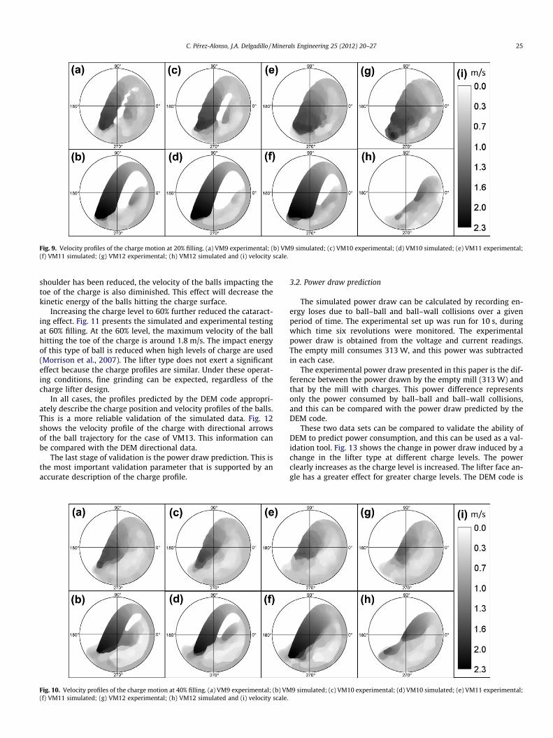
Fig. 9. Velocity profiles of the charge motion at 20% filling. (a) VM9 experimental; (b) VM9 simulated; (c) VM10 experimental; (d) VM10 simulated; (e) VM11 experimental;(f) VM11 simulated; (g) VM12 experimental; (h) VM12 simulated and (i) velocity scale.

C. Pérez-Alonso, J.A. Delgadillo / Minerals Engineering 25 (2012) 20–27 25

shoulder has been reduced, the velocity of the balls impacting thetoe of the charge is also diminished. This effect will decrease thekinetic energy of the balls hitting the charge surface.

Increasing the charge level to 60% further reduced the cataract-ing effect. Fig. 11 presents the simulated and experimental testingat 60% filling. At the 60% level, the maximum velocity of the ballhitting the toe of the charge is around 1.8 m/s. The impact energyof this type of ball is reduced when high levels of charge are used(Morrison et al., 2007). The lifter type does not exert a significanteffect because the charge profiles are similar. Under these operat-ing conditions, fine grinding can be expected, regardless of thecharge lifter design.

In all cases, the profiles predicted by the DEM code appropri-ately describe the charge position and velocity profiles of the balls.This is a more reliable validation of the simulated data. Fig. 12shows the velocity profile of the charge with directional arrowsof the ball trajectory for the case of VM13. This information canbe compared with the DEM directional data.

The last stage of validation is the power draw prediction. This isthe most important validation parameter that is supported by anaccurate description of the charge profile.

Fig. 10. Velocity profiles of the charge motion at 40% filling. (a) VM9 experimental; (b) VM(f) VM11 simulated; (g) VM12 experimental; (h) VM12 simulated and (i) velocity scale.

3.2. Power draw prediction

The simulated power draw can be calculated by recording en-ergy loses due to ball–ball and ball–wall collisions over a givenperiod of time. The experimental set up was run for 10 s, duringwhich time six revolutions were monitored. The experimentalpower draw is obtained from the voltage and current readings.The empty mill consumes 313 W, and this power was subtractedin each case.

The experimental power draw presented in this paper is the dif-ference between the power drawn by the empty mill (313 W) andthat by the mill with charges. This power difference representsonly the power consumed by ball–ball and ball–wall collisions,and this can be compared with the power draw predicted by theDEM code.

These two data sets can be compared to validate the ability ofDEM to predict power consumption, and this can be used as a val-idation tool. Fig. 13 shows the change in power draw induced by achange in the lifter type at different charge levels. The powerclearly increases as the charge level is increased. The lifter face an-gle has a greater effect for greater charge levels. The DEM code is

9 simulated; (c) VM10 experimental; (d) VM10 simulated; (e) VM11 experimental;

Fig. 11. Velocity profiles of the charge motion at 60% filling. (a) VM13 experimental; (b) VM13 simulated; (c) VM14 experimental; (d) VM14 simulated; (e) VM15experimental; (f) VM15 simulated; (g) VM16 experimental; (h) VM16 simulated and (i) velocity scale.

Fig. 12. Directional arrows for the measured velocities. (a) VM13 experimental profile, (b) VM13 simulated profile and (c) velocity scale.

26 C. Pérez-Alonso, J.A. Delgadillo / Minerals Engineering 25 (2012) 20–27

able to capture not only an accurate trajectory of the balls but alsoa good approximation of the power draw.

The power draw can be correlated as shown in Fig. 14, wherethe experimental (Exp) and simulated (Sim) data are plotted at dif-ferent operational conditions. The power draw calculations areaccurate and close to the experimental data. Datta and Rajamani(2002) and Datta et al. (1999) report good prediction of the power

Fig. 13. Variation of the power draw.

draw using a 3D code. This shows that the DEM is able to predictpower consumption in tumble mills.

When the charge level is from 40% to 60%, the simulation devi-ates from the experimental data on the order of 10%. This error isattributed to the lack of modeling in the third dimension. Never-theless, the simulations provide an excellent description of thepower draw of the system.

Fig. 14. Power draw prediction by DEM calculations.

C. Pérez-Alonso, J.A. Delgadillo / Minerals Engineering 25 (2012) 20–27 27

4. Conclusions

Digital image analysis is an excellent tool to measure systemparameters such as toe and shoulder angles and the ball velocityand location. These parameters provide enough experimental datato validate the DEM codes. The power draw is generally used tovalidate the codes, but this parameter can be easily fitted by simplychanging the model constants, whereas ball trajectory and velocityare not easy to compare with the experimental data. Most of thetools used to measure velocity profiles are difficult to use andexpensive. In contrast, digital image analysis can be applied at verylow cost and can precisely determine the trajectory and velocity ofthe balls in the system.

The code used in this work successfully predicts changes in thecharge using different lifter profiles and various charge levels. Thiscode can only predict the system in two dimensions with an accu-rate description of the trajectory and power draw. Some otherauthors (Nierop van et al., 2001; Rajamani et al., 2000) have shownthat 2D code gives an accurate description of the charge and canpredict larger mills where no direct observation of the charge ispossible. In industrial size mills, the power draw is the only vari-able that can be used to evaluate the quality of the simulation. Thiscode was validated for a laboratory ball mill but must be tested forpower draw prediction in industrial size mills.

Acknowledgment

The authors thank CONACyT for financial support through theProject SEP-CONACyT No. 83158 and scholarship No. 171419.

References

Austin, L.G., Klimpel, R.R., Luckie, P.T., 1984. Process engineering of size reduction:ball milling. Society of Mining Engineers, AIME, New York..

Buchholtz, V., Freund, J.A., Pöschel, T., 2000. Molecular dynamics of comminution inball mills. The European Physical Journal B 16, 169–182.

Cleary, P.W., 1998. Predicting charge motion, power draw, segregation, wear andparticle breakage in ball mills using discrete element methods. MineralsEngineering 11 (11), 1061–1080.

Cleary, P.W., 2000. DEM simulation of industrial particle flows: case studies ofdragline excavators, mixing in tumblers and centrifugal mills. PowderTechnology 109, 83–104.

Cleary, P.W., 2001a. Modelling comminution devices using DEM. Int. J. Numer.Annual. Methods Geomech. 25, 83–105.

Cleary, P.W., 2001b. Charge behavior and power consumption in ball mills:sensitivity to mill operating conditions, liner geometry and chargecomposition. International Journal of Mineral Processing 63, 79–114.

Cleary, P.W., 2009. Ball motion, axial segregation and power consumption in a fullscale two chamber cement mill. Minerals Engineering 22, 809–820.

Cleary, P.W., Hoyer, D., 2000. Centrifugal mill charge motion: comparison of DEMpredictions with experiment. International Journal of Mineral Processing 59,131–148.

Cleary, P.W., Morrison, R., Morrell, S., 2003. Comparison of DEM and experiment fora scale model SAG mill. International Journal of Mineral Processing 68, 129–165.

Datta, A., Rajamani, R.K., 2002. A direct approach of modeling batch grinding in ballmills using population balance principles and impact energy distribution.International Journal of Mineral Processing 64, 181–200.

Datta, A., Mishra, B.K., Rajamani, R.K., 1999. Analysis of power draw in ball mills bythe discrete element method. Canadian Metallurgical Quarterly 38 (2), 133–140.

Dong, H., Moys, M.H., 2002. Assessment of discrete element method for one ballbouncing in grinding mill. International Journal of Mineral Processing 65, 213–226.

Inoue, T., Okaya, K., 1995. Analysis of grinding actions of ball millas by discreteelement method. Proc. XIX Int. Min. Proc. Congress. Soc. Min., Metall. Explor 1,191–196.

Inoue, T., Okaya, K., 1996. Grinding mechanisms of centrifugal mills—a batchball mill simulator. International Journal of Mineral Processing 44 (45), 425–435.

Kano, J., Naoki, C., Saito, F., 1997. A method for simulating the three dimensionalmotion of balls under the presence of a powder sample in tumbling ball mill.Adv. Powder Technology 8 (1), 39–51.

Meijering, E., Jacob, M., Sarria, J.C.F., Steiner, P., Hirling, H., Unser, M., 2004. Designand Validation of a Tool for Neurite Tracing and Analysis in FluorescenceMicroscopy Images. Cytometry Part A 58 (2), 167–176.

Mishra, B.K., Study of media mechanics in tumbling mills. PhD Thesis. Departmentof Metallurgical Engineering, 1991, University of Utah.

Mishra, B.K. and Rajamani, R.K. (1990). Numerical simulation of charge motion inball mills. In: Proceedings of the 7th European Conference on Comminution,Ljubljan, Yugoslavia, pp. 555–570.

Mishra, B.K., Rajamani, R.K., 1992. The discrete element method for the simulationof ball mills. Appl. Math. Model. 16, 598–604.

Mishra, B.K., Rajamani, R.K., 1994a. Simulation of charge motion in ball mills. Part 1:experimental verifications. International Journal of Mineral Processing 40, 171–186.

Mishra, B.K., Rajamani, R.K., 1994b. Simulation of charge motion in ball mills.Part 2: numerical simulations. International Journal of Mineral Processing 40,187–197.

Morrison, R.D., Shi, F., Whyte, R., 2007. Modelling of incremental rock breakage byimpact – for use in DEM models. Minerals Engineering 20, 303–309.

Nierop van, M.A., Gover, G., Hinde, A.L., Moys, M.H., 2001. A discrete elementmethod investigation of the charge motion and power draw of an experimentaltwo-dimensional mill. International Journal of Mineral Processing 61, 77–92.

Powell, M.S., Nurick, G.N., 1996. A study of charge motion in rotary mills. Parts 1, 2,and 3. Minerals Engineering, 9 (3), 259–268; 343–350; 9 (4), 399–418.

Radziszewski, P., 1999. Comparing three DEM charge motion models. MineralsEngineering 12 (12), 1501–1520.

Rajamani, R.K., Mishra, B.K. (1996). Dynamics of ball and rock charge in SAG mills.Proc. SAG, Department of Mining and Mineral Process Engineering. Universityof British Columbia.

Rajamani, R.K., Mishra, B.K., Songfack, P., Venugopal, R., MILLSOFT—a simulationsoftware for tumbling mills design and troubleshooting. Minerals Engineering,1999, Dec., 41–47.

Rajamani, R.K., Mishra, B.K., Venugopal, R., Datta, A., 2000. Discrete element analysisof tumbling mills. Powder Technology 109, 105–112.

Venugopal, R., Rajamani, R.K., 2001. 3D simulation of charge motion in tumblingmills by the discrete element method. Powder Technology 115, 157–166.

Zhang, D., Whiten, W.J., 1996. The calculation of contact forces between particlesusing spring and damping models. Powder Technology 88, 59–64.

Zhang, D., Whiten, W.J., 1998. An efficient calculation method for particle motion indiscrete element simulations. Powder Technology 98, 223–230.