EXISTENCE OF COMMON ZEROS FOR COMMUTING VECTOR FIELDS …bruno_santiago/BS_Final.pdf · EXISTENCE OF COMMON ZEROS FOR COMMUTING VECTOR FIELDS ON THREE ... COMMUTING VECTOR FIELDS

Ann. Inst. Fourier, GrenobleWorking version – November 14, 2016

EXISTENCE OF COMMON ZEROS FOR COMMUTINGVECTOR FIELDS ON THREE MANIFOLDS

by Christian BONATTI and Bruno SANTIAGO (*)

Abstract. In 1964 E. Lima proved that commuting vector fields onsurfaces with non-zero Euler characteristic have common zeros. Suchstatement is empty in dimension 3, since all the Euler characteristicsvanish. Nevertheless, C. Bonatti proposed in 1992 a local version,replacing the Euler characteristic by the Poincaré-Hopf index of avector field X in a region U , denoted by Ind(X,U); he asked:

Given commuting vector fields X,Y and a region U whereInd(X,U) 6= 0

does U contain a common zero of X and Y ?A positive answer was given in the case where X and Y are real

analytic, in the same article where the above question was posed.In this paper, we prove the existence of common zeros for com-

muting C1 vector fields X, Y on a 3-manifold, in any region U suchthat Ind(X,U) 6= 0, assuming that the set of collinearity of X andY is contained in a smooth surface. This is a strong indication thatthe results for analytic vector fields should hold in the C1 setting.

Keywords: commuting vector fields, fixed points, Poincaré-Hopf index.Math. classification: 37C25, 37C85, 57S05, 58C30.(*) We thank Sebastien Alvarez for kind discussions helping to clean the argumentsand Johan Taflin for his kind interest in our work. We also thank Martin Vogel formany useful conversations. This work was supported by the Projeto Ciência Sem Fron-teiras Dinâmicas não hiperbolicas: aspectos topológicos e ergódicos (CAPES (Brazil))and by FAPERJ(Brazil). We thank the kind hospitality of Institut de Mathématiquesde Bourgogne, UMR 5584 du CNRS, Dijon, France and Departamento de Matemática,PUC-Rio de Janeiro, Brazil. The referee of the first version of this paper made a verycareful reading and provided many comments improving the text; we thank him/her.

2

Résumé. En 1964 E. Lima a montré que les champs de vecteursque commute dans une surface ont un zéro commun. Cette énonceest vide en dimension 3 puisque toutes les caractéristiques d’Eulersont nulles dans ce cas-là. Cependant, C. Bonatti a proposé 1992 uneversion locale, en remplaçant la caractéristique d’Euler par l’indicede Poincaré-Hopf d’un champ de vecteur X dans une région U , qu’ondenote par Ind(X,U). Il a proposé la question suivante: Étant donnédeux champs de vecteurs commutant X et Y et une région compacteU sur lequel

Ind(X,U) 6= 0,est-ce que U contient un zéro commun de X et Y ?

Une réponse positive a été donné dans le cas où X et Y sont réelleanalytique, dans le même papier où la question au-dessus a été posé.

Dans cet article on montre existence de zéros communs pour leschamps de vecteurs de classe C1 que commute en diménsion 3 pourchaque région U telle que l’indice Ind(X,U) est non nul et en sup-posent en plus que le lieu de colinéarité entre X et Y est contenudans une surface lisse. C’est une forte indication que le résultat pourles champs de vecteurs analytiques doit être vrai en régularité C1.

1. Introduction

One of the fundamental problems in dynamical systems is whether agiven system possesses fixed points or not. A simple scenario to pose thisquestion is for the Z-action generated by a diffeomorphism or a homeomor-phism of a manifold, or for the continuous time dynamical system generatedby the flow of a vector field. In both cases, the theories of Poincaré-Hopfand Lefschetz indices relate the topology of the ambient manifold with theexistence of fixed points.Nonetheless, if one consider two commuting diffeomorphisms or two com-

muting vector fields i.e. vector fields X and Y whose flows satisfy: (1)

Xt ◦ Ys = Ys ◦Xt, ∀(s, t) ∈ R2,

the existence of a fixed point for the action they generate is a wide openquestion in dimensions > 3.

The first result on this question is given by the works on surfaces ofLima [Li1], [Li2]. He proves that any family of commuting vector fields ona surface with non-zero Euler characteristic have a common zero. In thelate eighties, [Bo1] proved that commuting diffeomorphisms of the sphereS2 which are C1-close to the identity have a common fixed point. Later

(1)This definition can be adapted for non-complete vector fields, see Section 3

ANNALES DE L’INSTITUT FOURIER

COMMUTING VECTOR FIELDS ON THREE MANIFOLDS 3

[Bo2] extended this result to any surface with non-zero Euler characteris-tic (see other generalizations in [DFF][Fi]). Then, Handel [Ha] provided atopological invariant in Z/2Z for a pair of commuting diffeomorphisms ofthe sphere S2 whose vanishing guarantees a common fixed point. This wasfurther generalized by Franks, Handel and Parwani [FHP] for any num-ber of commuting diffeomorphisms on the sphere (see [Hi] and [FHP2] forgeneralizations on other surfaces).

It is worth to note, however, that two commuting continuous intervalmaps may fail to have a common fixed point: an example is constructed in[B] of two continuous commuting, non-injective, maps of the closed intervalwhich do not have a common fixed point.

In higher dimensions much less is known:

• One knows some relation between the topology of the manifold andthe dimension of the orbits of Rp-actions (see [MT1, MT2]). Thetechniques introduced in these works make possible a simple proofof Lima’s result, for smooth vector fields [Tu];

• [Bo3] proved that two commuting real analytic vector fields on ananalytic 4-manifold with non-zero Euler characteristic have a com-mon zero. The same statement does not make sense in dimensionthree since every 3-manifold has zero Euler characteristic. Never-theless, a local result remains true in dimension three.

Before stating the result of [Bo3] on 3-manifolds, we briefly recall thenotion of the Poincaré-Hopf index Ind(X,U) of a vector field X on a com-pact region U whose boundary ∂U is disjoint from the set Zero(X). If Uis a small compact neighborhood of an isolated zero p of the vector fieldX, then Ind(X,U) is just the classical Poincaré-Hopf index Ind(X, p) of Xat p. For a general compact region U with ∂U ∩ Zero(X) = ∅, one consid-ers a small perturbation Y of X with only finitely many isolated zeros inU . Then, we define the index Ind(X,U) as the sum of the Poincaré-Hopfindices Ind(Y, p), p ∈ Zero(Y ) ∩ U . We refer the reader to Section 3 fordetails (in particular for the fact that Ind(X,U) does not depend on theperturbation Y of X).Then, the main theorem of [Bo3] says that every pair X,Y of analytic

commuting vector fields have a common zero in any compact region U

such that Ind(X,U) 6= 0. By contraposition, if X and Y are analytic andcommute but do not have common zeros then Ind(X,U) = 0. By reducingthe compact region U so that it separates Zero(X) ∩ U from Zero(Y ) oneobtains the following statement:

SUBMITTED ARTICLE : BS_FINAL.TEX

4 CHRISTIAN BONATTI AND BRUNO SANTIAGO

Theorem 1.1 (Bonatti [Bo3]). — Let M be a real analytic 3-manifoldand X and Y be two analytic commuting vector fields over M . Let U be acompact subset of M such that Zero(Y ) ∩ U = Zero(X) ∩ ∂U = ∅. Then,

Ind(X,U) = 0.

This statement is also true whenM has dimension 2 and the vector fieldsare just C1 (see Proposition 11 in [Bo2](2) ). This motivates the following

Conjecture 1.2. — Let X and Y be two C1 commuting vector fieldson a 3-manifold M . Let U be a compact subset of M such that Zero(Y ) ∩U = Zero(X) ∩ ∂U = ∅.Then, Ind(X,U) = 0.

This conjecture was stated as a problem in [Bo3].The goal of the present paper is to solve, in the C1-setting, what was

the main difficulty in the analytic case in [Bo3]. We explain now what wasthis difficulty in [Bo3]. A crucial role is played by the set of points of U inwhich X and Y are collinear:

Col(X,Y, U) := {p ∈ U ; dim (〈X(p), Y (p)〉) 6 1}.

In [Bo3] the assumption that the commuting vector fields are analyticis used to say that Col(X,Y, U) is either equals to U or is an analyticset of dimension at most 2. The case where Col(X,Y, U) = U admits adirect proof. In the other case, a simple argument allows to assume thatCol(X,Y, U) is a surface. The main difficulty in [Bo3] consists in provingthat, if Col(X,Y, U) is a smooth surface and X and Y are analytic, thenthe index of X vanishes on U .Our result is the following

Theorem A. — Let M be a 3-manifold and X and Y be two C1 com-muting vector fields over M . Let U be a compact subset of M such thatZero(Y ) ∩ U = Zero(X) ∩ ∂U = ∅. Assume that Col(X,Y, U) is containedin a C1-surface which is a compact and boundaryless submanifold of M .Then,

Ind(X,U) = 0.

The hypothesis “ Col(X,Y, U) is contained in a C1-surface” consists inconsidering the simplest geometric configuration of Col(X,Y, U) for which

(2)The result stated in Proposition 11 of [Bo2] is for C∞ vector fields, but the proofindicated there can be adapted for C1 vector fields using cross-sections, in a similar waywe do here in Section 4



the conjecture is not trivial: if (X,Y ) is a counter example to the conjec-ture, then Col(X,Y ) cannot be “smaller” than a surface. More precisely,if Ind(X,U) 6= 0, and if Y commutes with X then the sets Zero(X − tY )for small t are not empty compact subsets of Col(X,Y, U), invariant bythe flow of Y and therefore consist in orbits of Y . If X and Y are as-sumed without common zeros, every set Zero(X − tY ) consists on regularorbits of Y , thus is a 1-dimensional lamination. Furthermore, these lamina-tions are pairwise disjoint and vary semi-continously with t. In particular,Col(X,Y, U) cannot be contained in a 1-dimensional submanifold of M .

Another (too) simple configuration would be the case where X and Y

are everywhere collinear. This case has been treated in [Bo3] and the sameproof holds at least in the C2 setting.We believe that the techniques that we introduce here will be usefull to

prove the conjecture, at least for C2 vector fields.

The proof of Theorem A is by contradiction. The intuitive idea whichguides the argument is that, at one hand, the vector field X needs to turnin all directions in a non-trivial way in order to have a non-zero index.On the other hand, X commutes with Y and therefore is invariant underthe tangent flow of a non-zero vector field. The combination of this twoproperties will lead to a contradiction.This paper is organized as follows.

• In Section 2 we give an informal presentation of the proof, describingthe main geometrical ideas.

• In Section 3 we give detailed definitions and state some classicalfacts that we shall use.

• In Section 4 we reduce the proof of Theorem A to the proof of aslightly more technical version of it (see Lemma 4.3), for which Uis a solid torus and Col(X,Y, U) is a annulus foliated by periodicorbits of Y , and cutting U in two connected components U+ andU−.

• In Section 5 we consider the projection N , of the vector field X

parallel to Y on the normal bundle of Y . We show that Ind(X,U)is related with the angular variations `+ and `− of N along gen-erators of the fundamental group of each connected componentsU+ and U− of U \ Col(X,Y, U). More precisely we will show inProposition 5.9 that

| Ind(X,U)| = |`+ − `−|.



Assuming that at least one of `+ and `− does not vanish, and thefact that Col(X,Y, U) is a C1-surface, we deduce in Proposition 5.19that the the first return map P of Y on a transversal Σ0 is C1-closeto identity in a small neighborhood of Col(X,Y, U) ∩ Σ0.

• In Section 6, still assuming that at least one of `+ and `− does notvanish, we give a description of the dynamics of the first return mapP. If for instance `+ 6= 0 then every point in Σ0 ∩ U+ belongs tothe stable set of a fixed point of P (Lemma 6.4). We will then usethe invariance of these stable sets under the orbits of the normalvector field N for getting a contradiction.

We end this introduction by a general comment. The accumulation ofresults proving the existence of common fixed points for commuting dy-namical systems seems to indicate the possibility of a general phenomenon.However, our approach in Poincaré-Bendixson spirit has a difficulty whichincreases drastically with the ambient dimension. We hope that this resultswill motivate other attempts to study this phenomenon.

2. Idea of the proof

The proof is by contradiction. We assume that there exists a counterexample to the Theorem, that is a pair of commuting C1-vector fields X,Yon a 3-manifold M , and a compact set U so that

• the colinearity locus of X and Y in U is contained in a closed C1

surface S in M .• X is non-vanishing on the boundary ∂U and the index Ind(X,U)is non-zero,

• X and Y have no comon zero in U .

Simplifying the counter examples. A first step of the proof (see thewhole Section 4 and more specifically Lemmas 4.1 and 4.3) consists inshowing that, up to shrink the compact set U , and up to replace the vectorfields X and Y by (constant) linear combinations of X and Y , one mayassume futher, without loss of generality, that

• the manifold M is orientable;• U is a solid torus D2 × (R/Z);• the surface S is an annulus invariant by the flow of X and Y whose

intersection with the boundary ∂U is precisely its own boundary∂S;



• Y is non-vanishing on U and transverse to every factor Σt = D2 ×{t}, t ∈ R/Z;

• for every x ∈ S its Y orbit is a periodic orbit contained in S, ofperiod τ(x).

• the map x ∈ S 7→ τ(x) > 0 is of class C1, constant on the Y -orbits,and its derivative is non vanishing on S;

• as X is colinear on S to the non-vanishing vector field Y one maywrite X(x) = µ(x)Y (x) for x ∈ S; then the map µ is of class C1,constant on the Y -orbits, and its derivative is non vanishing on S.

We endow the solid torus U with a basis B(x) = (e1(x), e2(x), e3(x)) ofTxM dependind continuously with x and so that e3(x) = Y (x), the plane< e1(x), e2(x) > is tangent to the disc Σt through x, and for x ∈ S thevector e1(x) is tangent to S.

Figure 2.1. Geometric configuration of a prepared counter exampleand the basis B(x) = (e1(x), e2(x), e3(x)) at a point x ∈ S ∩ Σt.

The pair of vector fields (X,Y ) with all these extra properties and en-dowed with the basis B is called a prepared counter example. More formallyLemmas 4.1 and 4.3 announce that the existence of a counter example toTheorem A implies the existence of a prepared counter example. The restof the proof consists in getting a contradiction from the existence of aprepared counter example.

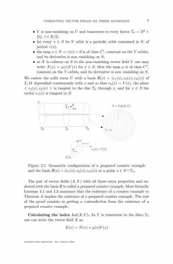
Calculating the index Ind(X,U). As Y is transverse to the discs Σtone can write the vector field X as

X(x) = N(x) + µ(x)Y (x)



where N(x) is a vector tangent to the discs Σt, so that one may writeN(x) = α(x)e1(x) + β(x)e2(x). This choice of coordinates allows us toconsider the vector N(x) as a vector on the plane R2. Notice that N(x)vanishes if and only if x ∈ S.

Thus, given any closed curve γ ⊂ U \ S which is freely homotopic to{(0, 0)}×(R/Z) in U , one defines the linking number of N along γ as beingthe number of turns given by N(x) (considered as a non-vanishing vectoron R2) as x runs along γ. One easily checks that this linking number onlydepends on the connected component of U \S which contains γ. Since U \Sconsist in two connected components U+ and U−, there are only two linkingnumbers which we denote by `+ and `− and we prove (Proposition 5.9)

| Ind(X,U)| = |`+ − `−|.

The normally hyperbolic case. By assumption the annulus S is fo-liated by periodic orbits of Y so that the derivative associated to theseperiodic orbits is 1 in the direction of S.Note that, if one of the periodic orbits of Y in S is partially hyperbolic,

that is, has an eigenvalue different from 1, then it admits a neighborhoodfoliated by the local stable manifolds of the nearby periodic orbits. Asthe vector field X commutes with Y and preserves each periodic orbit inS, it preserves each leaf of this foliation. Thus the normal vector N istangent to this foliation and one deduces that the linking numbers `+ and`− both vanish. Thus Ind(X,U) also vanishes leading to a contradiction(see Lemma 4.7 which formalizes this argument).

Figure 2.2. As X is tangent to the stable manifolds, it cannot turn inall directions. Its normal component N is everywhere collinear withe2, so that both linking numbers vanish.

The first return map P, the derivative of the return time, andthe angular variation of N . The vector field N does not commute with



Y but it is invariant under the holonomies of Y of the cross sections Σt. Onededuces that N almost cannot turn along the orbits of Y . This motivate usto calculate the linking number `± along particular closed curves obtainedin the following way: we follow the Y -orbit of a point x ∈ Σ0 \ S untilits first return P(x) then we close the curve by joining a small geodesicsegment in Σ0. This allows us to prove that the angular variation of N islarger than 2π along the segment in Σ0 joining x to P2(x) (second returnof x in Σ0) (Corollary 5.14).

Figure 2.3. N has large angular variation along the segments [x,P2(x)].

Now the contradiction we are looking for will be found in a subttle anal-ysis of the dynamics of the first return map P together with the dynamicsof the vector N , which commute together. In particular Corollary 5.6 linksthe direction of the vector field N(x) (through the derivative in the direc-tion of N of the return time of Y on Σ0) with the variation µ(P(x))−µ(x).The big angular variation of N along the small segments [x,P2(x)] lead usto prove that

• the derivative of P is the identity at any point of S (Proposi-tion 5.19)

• P almost preseves the levels of the map µ (see Lemmas 6.1 and6.2): one deduces that (up to exchange P by P−1) every orbit of Pconverges to a point of S.

Invariant stable sets and the contradiction. The second propertyabove allows us to obtain stable sets for the points in S ∩Σ0 (with respectto the first return map P) and to show that these stable sets are (as in thenormally hyperbolic case) invariant under the vecter field N . Unluckely theconcluison is not so straightforward as in the normally hyperbolic case. Wefirst prove that there is an N -orbit which is invariant uner P (Lemma 6.8)and we prove that the angular variation of N , between x and P2(x), along



such a P invariant N -orbit is arbitrarilly small when x is close to S ∩ Σ0:that is the announced contradiction.

3. Notations and definitions

In this paper M denotes a 3-dimensional manifold. Whenever X is avector field over M , we denote Zero(X) = {x ∈ M ;X(x) = 0} andZero(X,U) = Zero(X) ∩ U , for any subset U ⊂ M . We shall denote itsflow by Xt. A compact set Λ ⊂ M is invariant under the flow of X ifXt(Λ) = Λ for every t ∈ R.

If X and Y are vector fields on M we denote by Col(X,Y ) the set ofpoints p for which X(p) and Y (p) are collinear:

Col(X,Y ) = {p ∈M, dim(〈X(p), Y (p))〉 6 1}.

If U ⊂M is a compact region we denote Col(X,Y, U) = Col(X,Y ) ∩ U .

3.1. The Poincaré-Hopf index.

In this section we recall the classical definition and properties of thePoincaré-Hopf index.

Let X be a continuous vector field of a manifold M of dimension d andx ∈ M be an isolated zero of X. The Poincaré-Hopf index Ind(X,x)is defined as follows: consider local coordinates ϕ : U → Rd defined in aneighbohood U of x. Up to shrink U one may assume that x is the uniquezero of X in U . Thus for y ∈ U \ {x}, X(y) expressed in that coordinatesis a non vanishing vector of Rd, and 1

‖X(y)‖X(y) is a unit vector hencebelongs to the sphere Sd−1. Consider a small ball B centered at x. The mapy 7→ 1

‖X(y)‖X(y) induces a continuous map from the boundary S = ∂B toSd−1. The Poincaré-Hopf index Ind(X,x) is the topological degree of thismap.

Remark 3.1. — The Poincaré-Hopf index Ind(X,x) of an isolated zerox does not depend on a choice of a local orientation of the manifold at x.

For instance, the Poincaré Hopf index of a hyperbolic zero x is

Ind(X,x) = (−1)dimEs(x),

where Es(x) ⊂ TxM is the stable space of x.More conceptually, a change of the local orientation of M at x:



• composes the map x 7→ X(x)‖X(x)‖ with a symmetry of the sphere Sd−1

• changes the orientation of the sphere ∂B, where B is a small ballaround x.

Therefore the topological degre of the induced map from ∂B to Sd−1 iskept unchanged.

Assume now that U ⊂ M is a compact subset and that X does notvanish on the boundary ∂U . The Poincaré-Hopf index Ind(X,U) is definedas follows: consider a small perturbation Y of X so that the set of zerosof Y in U is finite. A classical result asserts that the sum of the indicesof the zeros of Y in U does not depend on the perturbation Y of X; thissum is the Poincaré-Hopf index Ind(X,U). Here, small perturbation meansthat Y is homotopic to X through vector fields which do not vanish on ∂U .More precisely

Proposition 3.2. — If {Xt}t∈[0,1] is a continuous family of vector fieldsso that Zero(Xt) ∩ ∂U = ∅, then Ind(Xt, U) does not depend on t ∈ [0, 1].

We say that a compact subset K ⊂ Zero(X) is isolated if there is acompact neighborhood U of K so that K = Zero(X)∩U ; the neighborhoodU is called an isolating neighborhood of K. The index Ind(X,U) does notdepend of the isolating neighborhood V of K. Thus Ind(X,U) is called theindex of K and denoted Ind(X,K).

3.2. Calculating the Poincaré Hopf index

Next Lemma 3.3 provides a practical method for calulating the index ofa vector field X in some region where it may have infinitely many zeros,without performing perturbations of X.Assume now that ∂U is a codimension one submanifold and that U is

endowed with d continous vector fields X1 . . . Xd so that, at every pointz ∈ U , (X1(z), . . . , Xd(z)) is a basis of the tangent space TzM . Once again,one can express the vector field X in this basis so that the vector X(y),for y ∈ U , can be considered as a vector of Rd. One defines in such a waya map g : ∂U → Sd−1 by y 7→ g(y) = 1

‖X(y)‖X(y).As ∂U has dimension d−1, and is oriented as the boundary of U , this map

has a topological degree. A classical result from homology theory impliesthe following

Lemma 3.3. — With the notations above the topological degre of g isInd(X,U).



In particular it does not depend on the choice of the vector fieldsX1 . . . Xd.

Remark 3.4. — By Lemma 3.3, if there is j ∈ {1, . . . , d} so that thevector X(x) is not colinear to Xj(x), for every x ∈ ∂U , then Ind(X,U) = 0.

3.3. Topological degree of a map from T2 to S2

We consider the sphere S2 (unit sphere of R3) endowed with the northand south poles denoted N = (0, 0, 1) and S = (0, 0,−1) respectively.We denote by S1 ⊂ S2 the equator, oriented as the unit circle of R2×{0}.

For p = (x, y, z) ∈ S2 \ {N,S} we call projection of p on S1 along themeridians the point 1√

x2+y2(x, y, 0), which is intersection of S1 with the

unique half meridian containing p.

Lemma 3.5. — Let Φ: S2 → S2 be a continuous map so that Φ−1(N) ={N} and Φ−1(S) = {S}.

Let ϕ : S1 → S1 be defined as follows: the point ϕ(p), for p ∈ S1, is theprojection of Φ(p) ∈ S2 \ {N,S} on S1 along the meridians of S2.Then the topopological degrees of Φ and ϕ are equal.

As a direct consequence one gets

Corollary 3.6. — Let Φ: S2 → S2 be a continuous map so thatΦ−1(N) = {S} and Φ−1(S) = {N}.

Let ϕ : S1 → S1 be defined as follows: the point ϕ(p), for p ∈ S1, is theprojection of Φ(p) ∈ S2 \ {N,S} on S1 along the meridians of S2.Then the topopological degrees of Φ and ϕ are opposite.

We consider now the torus T2 = R/Z×R/Z. As a direct consequence ofLemma 3.5 and Corollary 3.6 one gets:

Corollary 3.7. — Let Φ: T2 → S2 be a continuous map so thatΦ−1(N) = {0} × R/Z and Φ−1(S) = { 1

2} × R/Z.Let ϕ+ : { 1

4} × R/Z → S1 (resp. ϕ− : { 34} × R/Z → S1) be defined as

follows: the point ϕ+(p) (resp. ϕ−(p)) is the projection of Φ(p) ∈ S2\{N,S}on S1 along the meridians of S2.Then

|deg(Φ)| = |deg(ϕ+)− deg(ϕ−)|where deg() denotes the topological degree, and { 1

4}×R/Z and { 34}×R/Z

are endowed with the positive orientation of R/Z.

Proof. — Indeed, Φ is homotopic (by an homotopy preserving Φ−1(N)and Φ−1(S)) to the map Φd+,d− : R/Z× R/Z→ S2 defined as follows



• Φd+,d−(s, t) =(| sin(2πs)| · e2iπd+t, cos(2πs)

)if s ∈ [0, 1

2 ],

• Φd+,d−(s, t) =(| sin(2πs)| · e2iπd−t, cos(2πs)

)if s ∈ [0, 1

2 ].

where d+ and d− are deg(ϕ+) and deg(ϕ−), respectively. �

3.4. Commuting vector fields: local version

There are two usual definitions for commuting vector fields: we can re-quire that the flows of X and Y commute; one may also require that theLie bracket [X,Y ] vanishes. These two definitions coincide for C1 vectorfields on compact manifolds. On non compact manifolds we just have thecommutation of the flows for small times, as explained more precisely be-low.Let M be a (not necessarily compact) manifold and X, Y be C1-vector

fields on M . The Cauchy-Lipschitz theorem asserts that the flow of X andY are locally defined but they may not be complete.We say that X and Y commute if for every point x there is t(x) > 0 so

that for every s, t ∈ [−t(x), t(x)] the compositions Xt ◦Ys(x) and Ys ◦Xt(x)are defined and coincide. Thus, the local diffeomorphism Xt carries integralcurves of Y into integral curves of Y , and vice-versa.

Remark 3.8. — There are (non complete) commuting vector fields, apoint x and t > 0 and s > 0 so that both Xt ◦ Ys(x) and Ys ◦ Xt(x) aredefined but are different. Let us present an example.Consider C∗ = R2 \ {(0, 0)} endowed with the two vector fields X = ∂

∂x

and Y = ∂∂y . Note that X and Y commute. Consider the 2-cover φ : C∗ →

C∗ defined by z 7→ z2. Let X and Y the lifts for φ of X and Y , respectively.Then X and Y commute. However, consider the point x = (− 1√

2 ,−1√2 ) =

eiπ54 . Consider x = eiπ

58 , so that φ(x) = x.

Next figure illustates the fact that XtYt(x) and YtXt(x) are well definedbut distinct, for t =

√2:

Next section states straightforward consequences of this definition.

3.5. Commuting vector fields: first properties

If X and Y are commuting vector fields then:(1) for every a, b, c, d ∈ R, aX + bY commutes with cX + dY ;



Figure 3.1. The flow X commutes with the flow of Y until one of thecomposed orbits XtYs crosses one of the axes.

(2) for every x ∈M , and any t ∈ R for which Yt is defined, one has

DYt(x)X(x) = X(Yt(x))

(3) if x ∈ Zero(X), Then for any t ∈ R for which Yt is defined, Yt(x) ∈Zero(X).

(4) Col(X,Y ) is invariant under the flow of X in the following meaning:if x ∈ Col(X,Y ) and if Xt(x) is defined, then Xt(x) ∈ Col(X,Y );in the same way, Col(X,Y ) is invariant under the flow of aX + bY

for any a, b ∈ R.(5) if Zero(Y ) = ∅, Then for each point x in Col(X,Y ) there is µ(x) ∈ R

so that X(x) = µ(x)Y (x). The map x 7→ µ(x) is called the ratiobetween X and Y at x and is continuous on Col(X,Y ) and can beextended in a C1 map on the ambient manifold.Proof. — One can extend µ to a small neighboorhod V of Col(X,Y )

in the following way: given some riemannien metric on M , if V issmall enough then X is never orthogonal to X in V \ Col(X,Y ).Thus, one can consider the vector field Z obtained as the orthogonalprojection of X onto the direction of Y . It is clear that Z|Col(X,Y ) =X and that there exists a C1 function ψ : V → R such thatZ(x) = ψ(x)Y (x). Since Zero(Y ) = ∅, this implies that ψ is anextension of µ. Moreover, clearly ψ extends to M .(3) �

(6) the ratio µ defined on Col(X,Y ) is invariant under the flow of aX+bY for any a, b ∈ R.

(7) if γ is a periodic orbit of X of period τ and if t ∈ R is such that Ytis defined on γ, then Yt(γ) is a periodic orbit of X of period τ . The

(3)We shall see in Section 5 a particular case of this construction.



same occurs with the images by the flow of cX + dY of periodicorbits of aX + bY , for a, b, c, d ∈ R.

(8) as a consequence of the previous item, if γ is a periodic orbit of Xof period τ and if γ is isolated among the periodic orbits of X ofthe same period τ , then γ is invariant under the flow of Y ; as aconsequence, γ ⊂ Col(X,Y ).

3.6. Counter examples to Theorem A

Our proof is a long proof by reductio ad absurdum. To achieve this goal,we shall first show that the existence of a pair (X,Y ) which do not sat-isfy the conclusion of Theorem A implies the existence of other pairs withsimpler geometric behaviors.For this reason, it will be convenient to define the notion of counter

examples in a formal manner.

Definition 3.9. — Let M be a 3-manifold, U a compact subset of Mand X, Y be C1 vector fields on M . We say that (U,X, Y ) is a counterexample to Theorem A if

• X and Y commute• Zero(Y ) ∩ U = ∅• Zero(X) ∩ ∂U = ∅• Ind(X,U) 6= 0.• the collinearity locus, Col(X,Y, U), is contained in a C1 surface

which is a closed submanifold of M .

Let us illustrate our simplifying procedure by a simple argument:

Remark 3.10. — If M is a 3-manifold carrying a counter example

(U,X, Y )

to Theorem A, then there is an orientable manifold carrying a counterexample to Theorem A. Indeed, consider the orientation cover M → M

and U , X, Y the lifts of U,X, Y on M . Then the Poincaré-Hopf index of Xon U is twice the one of X on U , and (U , X, Y ) is a counter example toTheorem A.

Thus we can assume (and we do it) without loss of generality that M isorientable.Most of our simplifying strategy will now consist in combinations of the

following remarks



Remark 3.11. — If (U,X, Y ) is a counter example to Theorem A, thenthere is ε > 0 so that (U, aX + bY, cX + dY ) is also a counter exampleto Theorem A, for every a, b, c, d with |a − 1| < ε, |b| < ε, |c| < ε and|d− 1| < ε.

Remark 3.12. — If (U,X, Y ) is a counter example to Theorem A, then(V,X, Y ) is also a counter example to Theorem A for any compact setV ⊂ U containing Zero(X,U) in its interior.

Remark 3.13. — Let (U,X, Y ) be a counter example to Theorem A andassume that Zero(X,U) = K1∪· · ·∪Kn, where the Ki are pairwise disjointcompact sets. Let Ui ⊂ U be compact neighborhood of Ki so that the Ui,i = 1, . . . , n, are pairwise disjoint.Then there is i ∈ {1, . . . , n} so that (Ui, X, Y ) is a counter example to

Theorem A.

4. Prepared counter examples (U,X, Y ) to Theorem A

Simplifying Col(X,Y, U). The aim of this paragraph is to prove

Lemma 4.1. — If (U,X, Y ) is a counter example to Theorem A thenthere is a counter example (U , X, Y ) to Theorem A and µ0 > 0 with thefollowing property:

• for any t ∈ [−µ0, µ0], the set of zeros of X − tY in U consistsprecisely in 1 periodic orbit γt of Y ;

• for any t /∈ [−µ0, µ0], the set of zeros of X − tY in U is empty;• Col(X, Y , U) is a C1 annulus;• there is a C1-diffeomorphism ϕ : R/Z × [−µ0, µ0] → Col(X, Y , U)so that, for every t ∈ [−µ0, µ0], one has

ϕ(R/Z× {t}) = γt.

Proof. — By hypothesis Col(X,Y, U) is contained in a C1-surface S.Notice that there is µ1 > 0 so that for any t ∈ [−µ1, µ1] one has Zero(X −tY )∩∂U = ∅ and Ind(X−tY, U) 6= 0. In particular, we have that Zero(X−tY, U) 6= ∅.As X − tY and Y commute, Zero(X − tY, U) is invariant under the flow

of Y . Futhermore, as Zero(X − tY ) does not intersect ∂U the Y -orbit of apoint x ∈ Zero(X− tY, U) remains in the compact set U hence is complete.

Consider now the ratio function µ : Col(X,Y )→ R, defined in the item(5) of Subsection 3.5. It follows that, for x ∈ Col(X,Y ), µ(x) = t ⇔ x ∈



Zero(X − tY ). The map µ is invariant under the flows of X and Y (onCol(X,Y )). As mentioned in 3.5, the map µ can be extended on M as C1

map still denoted µ (but no more X,Y -invariant).Let L =

⋃t∈[−µ1,µ1] Zero(X−tY )∩U . Then L is a compact set, contained

in S disjoint from the boundary of U and invariant under Y : it is a compactlamination of S.By applying the flox box theorem and a standard compactness argument

we can take σ ⊂ S a union of finitely many compact segments with endpoints out of L and so that the interior of σ cuts transversely every orbitof Y contained in L.

Claim 1. — Lebesgue almost every t ∈ [−µ1, µ1] is a regular value ofthe restriction of µ to σ.

Proof. — Recall that Sard’s theorem requires a regularity n − m + 1if one consider maps from an m-manifold to an n-manifold. As µ is C1

and dim σ = 1 we can apply Sard’s theorem to the restriction of µ to σ,concluding. �

Consider now a regular value t ∈ (−µ1, µ1) of the restriction of µ to σ.Then µ−1(t) ∩ σ consists in finitely many points. Furthermore, µ−1(t) ∩ σcontains Zero(X − tY ) ∩ σ.

Claim 2. — For t ∈ [−µ1, µ1], regular value of the restriction of µ to σ,the compact set Zero(X − tY )∩U consists in finitely many periodic orbitsγi, i ∈ {1, . . . , n} of Y .

Proof. — Zero(X − tY ) ∩ U is a compact sub lamination of L ⊂ S con-sisting of orbits of Y , and contained in µ−1(t). Now, σ cuts transverselyeach orbit of this lamination and σ ∩ µ−1(t) is finite. One deduces thatZero(X− tY )∩U consists in finitely many compact leaves, concluding. �

We now fix a regular value t ∈ (−µ1, µ1) of the restriction of µ to σ.Since Zero(X − tY, U) 6= ∅ we have that the integer n of the above claim

is positive. Moreover, notice that Ind(X − tY, U) =∑ni=1 Ind(X − tY, γi).

Thus there is i so that

Ind(X − tY, γi) 6= 0.

Claim 3. — There is a neighborhood Γi of γi in S which is containedin Col(X,Y, U) and which consists in periodic orbits of Y .

Proof. — Let p be a point in σ ∩ γi. As p is a regular point of therestriction of µ to σ there is a segment I ⊂ σ centered at p so that therestriction of µ to I is injective and the derivative of µ does not vanish.



As γi has non-zero index for any s close enough to t, Zero(X − sY )contains an isolated compact subset Ks contained in a small neighborhoodof γi, and hence in U , thus in Col(X,Y, U) and thus in a small neighborhoodof γi in L ⊂ S. This implies that each orbit of Y contained in Ks cuts I.However, µ is constant equal to s on Ks and thus µ−1(s) ∩ I consist in aunique point. One deduces that Ks is a compact orbit of Y .Since this holds for any s close to t, one obtain that any point q of I close

to p is the intersection point of Kµ(q) ∩ I. In other words, a neighborhoodof p in I is contained in Col(X,Y, U) and the corresponding leaf of L is aperiodic orbit of Y , concluding. �

Notice that Γi is contained in Col(X,Y, U) so that the function µ isinvariant under Y on Γi. As the derivative of µ is non vanishing (by con-struction) on Γi ∩ I one gets that the derivative of the restriction of µ toΓi is non-vanishing. One deduces that Γi is diffeomorphic to an annulus: itis foliated by circles and these circles admit a transverse orientation.For concluding the proof it remains fix t ∈ (−µ1, µ1) regular value of µ,

then one fixes X = X − tY and Y = Y . One chooses a compact neighbor-hood U of γi in M , which is a manifold with boundary, whose boundary istranverse to S and so that U ∩S = Γi. By construction, (U , X, Y ) satisfiesall the announced properties. �

4.1. Prepared counter examples to Theorem A

Definition 4.2. — We say that (U,X, Y,Σ,B) is a prepared counterexample to Theorem A if

(1) (U,X, Y ) is a counter example to Theorem A(2) There is µ0 > 0 so that (U,X, Y ) satisfies the conclusion of Lemma 4.1:

• for any t ∈ [−µ0, µ0], the set of zeros of X − tY in U consistsprecisely in 1 periodic orbit γt of Y ;

• for any t /∈ [−µ0, µ0], the set of zeros of X − tY in U is empty;• Col(X,Y, U) is a C1 annulus;• there is a C1-diffeomorphism ϕ : R/Z×[−µ0, µ0]→ Col(X,Y, U)so that, for every t ∈ [−µ0, µ0], one has

ϕ(R/Z× {t}) = γt.

(3) U is endowed with a foliation by discs; more precisly there is asmooth submersion Σ: U → R/Z whose fibers Σt = Σ−1(t) arediscs; furthermore, the vector field Y is transverse to the fibers Σt.



(4) Each periodic orbit γs, s ∈ [−µ0, µ0], of Y cuts every disc Σt inexactly one point. In particular the period of γs coincides with itsreturn time on Σ0 and is denoted τ(s), for s ∈ [−µ0, µ0].Thus s 7→ τ(s) is a C1-map on [−µ0, µ0]. We require that the

derivative of τ does not vanish on [−µ0, µ0].(5) B is a triple (e1, e2, e3) of C0 vector fields on U so that

• for any x ∈ U B(x) = (e1(x), e2(x), e3(x)) is a basis of TxU .• e3 = Y everywhere• the vectors e1, e2 are tangent to the fibers Σt, t ∈ R/Z. Inother words, DΣ(e1) = DΣ(e2) = 0

• The vector e1 is tangent to Col(X,Y ) at each point of Col(X,Y ).

Lemma 4.3. — If there exists a counter example (U,X, Y ) to Theo-rem A then there is a prepared counter example (U , X, Y ,Σ,B) to Theo-rem A.

Proof. — The two first items of the definition of prepared counter exam-ple to Theorem A are given by Lemma 4.1. For getting the third item, itis enough to shrink U . For getting item (4), one replace Y by Y + bX forsome b ∈ R, |b| small enough. This does not change the orbits γt, as X andY are both tangent to γt, but it changes its period. Thus, this allows us tochange the derivative of the period τ at s = 0. Then one shrink again U

and µ0 so that the derivative of τ will not vanish on Col (X,Y, U).Consider any metric on U . For any point x in the annulus Col(X,Y, U)

and contained in the fiber Σt we chose e1(x) as being a unit vector tangentto the segment Col(X,Y ) ∩ Σt. We extend e1 as a continuous vector fieldon U tangent to the fibers Σt. We choose e2(x), for any x in a fiber Σt asbeing an unit vector tangent to Σt and orthogonal to e1(x). Now e3(x) =Y (x) is transverse to the plane spanned by e1(x), e2(x) so that B(x) =(e1(x), e2(x), e2(x)) is a basis of TxM . This provides the basis announcedin item 5. �

Remark 4.4. — If (U,X, Y,Σ,B) is a prepared counter example to The-orem A, then for every t ∈ (−µ0, µ0), (U,X − tY, Y,Σ,B) is a preparedcounter example to Theorem A.

Whenever (U,X, Y,Σ,B) is a prepared counter example to Theorem A,we shall denote by P the first return map, defined on a neighborhood ofCol(X,Y ) ∩ Σ0 in Σ0.

Remark 4.5. — As the ambient manifold is assumed to be orientable(see Remark 3.10), the vector field Y is normally oriented so that thePoincaré map P preserves the orientation.



4.2. Counting the index of a prepared counter example

Definition 4.6. — Let (U,X, Y,Σ,B) be a prepared counter exampleto Theorem A. In particular, U is a solid torus (C1-diffeomorphic to D2 ×R/Z) and Zero(X − tY ), t ∈ (−µ0, µ0), is an essential simple curve γtisotopic to {0} × R/Z. An essential torus T is the image of a continuousmap from the torus T2 in the interior of U , disjoint from γ0 = Zero(X) andhomotopic, in U \ γ0, to the boundary of a tubular neighborhood of γ0.

In other words, H2(U \γ0,Z) = Z, and T is essential if it is the generatorof this second homology group.We shall now describe how we use the basis B, which comes with a

prepared counter example, and an essential torus T to calculate the index.For each point x ∈ U , one can write X(x) as a linear combination of

the vectors e1(x), e2(x) and e3(x). Notice that, since e3 = Y everywhere,the e3-coordinate µ of X is a C1 extension of the ratio function, µ thatwe introduced on Col(X,Y ) in item (5) of Subsection 3.5. Therefore, thereexists C1 functions α, β, µ : U → R such that

(4.1) X(x) = α(x)e1(x) + β(x)e2(x) + µ(x)e3(x).

For x /∈ γ0 one considers the vector

(4.2) X (x) = 1√α(x)2 + β(x)2 + µ(x)2

(α(x), β(x), µ(x)) ∈ S2.

The map restriction X|T : T → S2 has a topological degree, which, byLemma 3.3, coincides with Ind(X,U), for some choice of an orientation onT .

4.3. The normally hyperbolic case

In this section we illustrate our procedure by giving the very simple proofof Theorem A in the case where Col(X,Y, U) is furthermore assumed to benormally hyperbolic for the flow of Y .

Here we shall prove

Lemma 4.7. — Let (U,X, Y,Σ,B) be a prepared counter example toTheorem A. Then, the first return map P : Σ0 → Σ0 of the flow of Ysatisfies: for every point x of Col(X,Y, U) ∩ Σ0, the unique eigenvalue ofthe derivative of P at x is 1.



Proof. — The argument is by contradiction. Let us denote xt = γt ∩Σ0,t ∈ [−µ0, µ0], (recall γt = Zero(X − tY )). We assume that the derivativeof P at some point of xt0 has some eigenvalue of different from 1.Notice that the first return map P is the identity map in restriction to

the segment Col(X,Y )∩Σ0. In particular, the derivative of P at xt admits1 as an eigenvalue. Since P preserves the orientation (see Remark 4.5), theother eigenvalue is positive.

Claim 4. — There exists U ⊂ U , X = X − tY and a prepared counterexample to Theorem A (U , X, Y,Σ,B) for which the surface Col(X, Y, U)is normally hyperbolic.

Proof. — As the property of having a eingenvalue of mudulus differentfrom 1 is an open condition, there exists an interval [µ1, µ2] ⊂ [−µ0, µ0] onwhich the condition holds. Consider t = µ1+µ2

2 and X = X − tY .Then, one obtains a new prepared counter example to Theorem A by

replacing X by X (see Remark 4.4); now, by shrinking U one gets a tubularneighborhood U of γt so that Col(X, Y, U) =

⋃s∈[µ1,µ2] γs.

Moreover, the derivative of P at each point xs, s ∈ [µ1, µ2], has aneigenvalue different from 1 in a direction tranverse to Col(X, Y, U) ∩ Σ0.By compactness and continuity these eigenvalues are uniformly far from 1so that Col(X, Y, U) ∩ Σ0 is normally hyperbolic for P.Thus Col(X, Y, U) is an invariant normally hyperbolic annulus for the

flow of Y . �

By virtue of the above claim (up to change X by X and U by U) onemay assume that Col(X,Y, U) is normally hyperbolic, and (up change Yby −Y ) one may assume that Col(X,Y, U) is normally contracting.This implies that every periodic orbit γt has a local stable manifold

W sY (γt) which is a C1-surface depending continuously on t for the C1-

topology and the collection of these surfaces build a C0-foliation FsY tan-gent to a continuous plane field EsY , in a neighborhood of Col(X,Y, U).Furthermore, EsY is tangent to Y , and hence is tranverse to the fibers of Σ.

Up to shrink U , one may assume that FsY and EsY are defined on U .

Claim 5. — There is a basis B = (e1, e2, e3) so that (U,X, Y,Σ, B) is aprepared counter example to Theorem A and e2 is tangent to EsY .

Proof. — Choose e2 as being a unit vector tangent to the intersectionof EsY with the tangent plane of the fibers of Σ. It remains to choose e1tranverse to e2 and tangent to the fibers of Σ and tangent to Col(X,Y ) atevery point of Col(X,Y ). �



Up to change B by the basis B given by the claim above, we will nowassume that e2 is tangent to EsY .

Claim 6. — The vector field X is tangent to EsY .

Proof. — The flow of the vector field X leaves invariant the periodicorbit γt of Y and X commutes with Y . As a consequence, it preserves thestable manifold W s(γt) for every t. This implies that X is tangent to thefoliation FsY and therefore to EsY . �

Therefore, for every x ∈ U \Zero(X) the vector X (x) ∈ S2 (see the nota-tions in Equations 4.1 and 4.2) belongs to the circle {x1 = 0}. In particular,for any essential torus T the map X|T : T → S2 is not surjective, an thushas zero topological degree. This proves that Ind(X,U) vanishes, contra-dicting the fact that (U,X, Y,Σ,B) is assumed to be a prepared counterexample to Theorem A. �

5. Holonomies, return time, and the normal component

In the whole section, (U,X, Y,Σ,B) is a prepared counter example toTheorem A.

Definitions. Recall that Σt = Σ−1(t), t ∈ R/Z, is a family of crosssection, each Σt is diffeomorphic to a disc, and we identify Σ0 with theunit disc D2.

Definition 5.1. — Consider t ∈ R. Consider x ∈ Σ0 and y ∈ Σt. Wesay that y is the image by holonomy of Y over the segment [0, t], and wedenote y = Pt(x), if there exists a continuous path xr ∈ U , r ∈ [0, t], sothat Σ(xr) = r, x0 = x, xt = y, and for every r ∈ [0, t] the point xr belongsto the Y -orbit of x.

The holonomy map Pt is well defined in a neighborhood of Col(X,Y, U)∩Σ0 and is a C1 local diffeomorphism.If t = 1 then P1 is the first return map P (defined before Remark 4.5) of

the flow of Y on the cross section Σ0.

Remark 5.2. — With the notation of Definition 5.1, there is a uniquecontinuous function τx : [0, t]→ R so that τx(0) = 0 and xr = Yτx(r)(x) forevery r ∈ [0, t].We denote τt(x) = τx(t) and we call it the transition time from Σ0 to

Σt. The map τt : Σ0 → R is a C1 map and by definition one has

(5.1) Pt(x) = Yτt(x)(x)



We denote τ = τ1 and we call it the first return time of Y on Σ0.Remark 5.3. — In Definition 4.2 item 4 we defined τ(s) as the period

of γs; in the notation above, it coincides with τ(xs) where xs = γs ∩ Σ0.In this case, Equation 5.1 takes the special form

(5.2) P(x) = Yτ(x)(x)

5.1. The normal conponent of X

Definition 5.4. — For every t and every x ∈ Σt we define the normalcomponent of X, which we denote by N(x), the projection of X(x) on TxΣtparallel to Y (x).

Thus x 7→ N(x) is a C1-vector field tangent to the fibers of Σ and whichvanishes precisely on Col(X,Y, U).Moreover, in the basis B, N(x) = α(x)e1(x) + β(x)e2(x) (see Equa-

tion 4.1), and we have the following formula

X(x) = N(x) + µ(x)Y (x),

for every x ∈ U .

The first return map and the derivative of the first return time.The goal of this paragraph is the proof of Corollary 5.6 which claims thefollowing formula

(5.3) −Dτ(x)N(x) = µ((P(x)))− µ(x)

relating the derivative of the return time function τ : Σ0 → (0,+∞), thenormal component N and the first return map P, at every point x ∈ Σ0.This formula will be crucial for transfering informations on the normal vec-tor field N to the first return map P. At the end of this section, we shall usethe angular variation of N (see the precise formulation in Corollary 5.14)together with formula (5.3) to prove that the derivative of P at any fixedpoint is the identity.The geometrical idea for proving (5.3) is the following:• at one hand, if x ∈ Σ0, one has that the difference between thevectors DP(x)N(x) and DYτ(x)(x)N(x) is parallel to Y (P(x)), andthe proportion is given exactly by Dτ(x)N(x) (this is a classicalfact, which we state precisely below).

• On the other hand, X is equal to N + µY and is invariant underDYt, for any t.



Figure 5.1. Geometric proof of formula (5.3):N(P(x)) + µ(P(x))Y (P(x)) = X(P(x)) = DYτ(x)(x)N(x) + µ(x)Y (P(x))

thus Dτ(x)N(x)Y (P(x)) = (µ(x)− µ(P(x)))Y (P(x))

One gets (5.3) by combining these two facts.Let us proceed with the formal proof. The first step is the (classical)

result below. The proof is an elementary and simple application of the flowbox theorem, so we omit.

Lemma 5.5. — For every t ∈ R x ∈ Σ0 and every v ∈ TxΣ0 one has,

(5.4) DPt(x)v −DYτt(x)(x)v = Dτt(x)v.Y (Pt(x)).

In particular, for every x ∈ Σ0 and v ∈ TxΣ0, one has

(5.5) DP(x)v −DYτ(x)(x)v = Dτ(x)v.Y (P(x)).

Now, recall thatX(x) = N(x) + µ(x)Y (x)

and sinceDYτ(x)X(x) = X(Yτ(x)) = X(P(x)),

we obtain

(5.6) X(P(x)) = DYτ(x)(x)N(x) + µ(x)Y (P(x)).

On the other hand, by Lemma 5.5

DYτ(x)(x)N(x) = DP(x)N(x)−Dτ(x)N(x)Y (P(x)).



AsX(P(x)) = N(P(x)) + µ(P(x))Y (P(x)),

we conclude that

DP(x)N(x)−Dτ(x)N(x))Y (P(x)) + µ(x)Y (P(x))= N(P(x)) + µ(P(x))Y (P(x)),

and so

(µ(x)− µ(P(x))−Dτ(x)N(x)))Y (P(x)) +DP(x)N(x)−N(P(x)) = 0.

Since Y is transverse to the tangent space of Σ0, the vectors Y (P(x)) andDP(x)N(x) − N(P(x)) are linearly independent. As a consequence, oneobtains that DP(x)N(x) = N(P(x)) and

Corollary 5.6. — Let x ∈ Σ0. Then,

−Dτ(x)N(x) = µ((P(x)))− µ(x).

Moreover, applying the same argument with the time t holonomy Pt inplace of the first return map P, one obtain the invariance of N under theholonomies.

Lemma 5.7. — For t ∈ R and every x ∈ Σ0 one has

DPt(x)N(x) = N(Pt(x)).

The normal component of X and the index of X. Let (U,X, Y,Σ,B)be a prepared counter example to Theorem A and N be the normal com-ponent of X.

Let us define, for x ∈ U \ Col (X,Y, U),

N (x) = 1√α(x)2 + β(x)2

(α(x), β(x)) ∈ S1 ⊂ S2,

where S1 is the unit circle of the plane R2 × {0} ⊂ R3.Recall that U is homeomorphic to the solid torus so that its first ho-

mology group H1(U,Z) is isomorphic to Z, by an isomorphism sending theclass of γ0, oriented by Y , on 1. Let U+ and U− be the two connected com-ponents of U \Col (X,Y, U). These are also solid tori, and the inclusion inU induces isomorphisms of the first homology groups which allows us toidentify H1(U±,Z) with Z.

Definition 5.8. — We call linking number of X with respect to Y inU+ (resp. in U−) and we denote it by `+(X,Y ) (resp. `−(X,Y )) the integerdefined as follows: the continuous map N : U± → S1 induces morphisms on



the homology groups H1(U±,Z)→ H1(S1,Z). As these groups are all iden-tified with Z, these morphisms consist in the multiplication by an integer`±(X,Y ).

In other words, consider a closed curve σ ⊂ U+ homotopic in U to γ0.Then `+(X,Y ) is the topological degree of the restriction of N to σ.

Proposition 5.9. — Let (U,X, Y,Σ,B) be a prepared counter exampleto Theorem A. Then

| Ind(X,U)| = |`+(X,Y )− `−(X,Y )|

Proof. — Consider a tubular neighborhood of γ0 whose boundary is anessential torus T which cuts Col (X,Y, U) transversely and along exactlytwo curves σ+ and σ−. Then the map X on T takes the value N ∈ S2

(resp. S ∈ S2) exactly on σ+ (resp. σ−), where N and S are the points onS2 corresponding to e3 = Y and −e3.We identify T with T2 = R/Z × R/Z so that σ− and σ+ correspond to

{ 12} × R/Z and {0} × R/Z respectively. It remains to apply Corollary 3.7

to Φ = X and ϕ = N , noticing that N is the projection of X on S1 alongthe meridians. This gives the announced formula. �

As a direct consequence of Proposition 5.9 one gets

Corollary 5.10. — Let (U,X, Y,Σ,B) be a prepared counter exampleto Theorem A, then

(`+(X,Y ), `−(X,Y )) 6= (0, 0)

5.2. Angular variation of the normal component

Definition of the angular variation. Recall that, for any x ∈ U \Col(X,Y ), we defined N (x) ∈ S1 as the expression in the basis B(x) of therenormalization of the normal component N(x).Consider a path η : [0, 1]→ U\Col(X,Y ). We define the angular variation

of N along η is as being

N (η(1))− N (η(0))

where N (η(t)) is a lift of the path t 7→ N (η(t) ∈ S1 on the universal coverR 7→ S1 ' R/2πZ.

By a practical abuse of language, if there is no ambiguity on the basisB, we will call angular variation of N along η the angular variation of Nalong η.



Angular variation of the normal component N along the Y -orbits. We denote {xt} = γt ∩ Σ0. For every pair of points x, y ∈ Σ0, wedenote the segment of straight line joinning x and y and contained in Σ0by [x, y] (for some choice of coordinates on Σ0).

Lemma 5.11. — For any K > 0 there is a neighborhood VK of γ0 withthe following property.Consider x ∈ VK ∩ Σ0 and u ∈ TxΣ0 a unit vector, and write u =

u1e1(x)+u2e2(x). Consider t ∈ [0,K] and v = DPt(u) ∈ TPt(x)Σt the imageof u by the derivative of the holonomy. Write v = v1e1(Pt(x))+v2e2(Pt(x)).Then (

u1√u2

1 + u22,

u2√u2

1 + u22

)6= −

(v1√v2

1 + v22,

v2√v2

1 + v22

)Proof. — Assuming, by contradiction, that the conclusion does not hold

we get yn ∈ Σ0, unit vectors un ∈ TxnΣ0 and tn ∈ [0,K] so that yn tends

to x0 = γ0∩Σ0, un tends to a unit vector u in Tx0Σ0, tn tends to t ∈ [0,K]and the image vn of the vector un, expressed in the basis B, is collinear toun with the opposite direction.

Then DPt(x0)u is a vector that, expressed in the basis B, is collinear to uwith the opposit direction. In other words, u is an eigenvector of DPt(x0),with a negative eigenvalue.However, for every t ∈ R the vector e1 is an eigenvector of DPt(x0), with

a positive eigenvalue, and DPt(x0) preserves the orientation, leading to acontradiction. �

Lemma 5.12. — For every N ∈ N there exists a neighborhood ON ⊂ Σ0of x0 so that if x ∈ ON \ Col(X,Y, U) then the segment of straight line[x,PN (x)] is disjoint from Col(X,Y, U).

Proof. — Assume that there is a sequence of points yn → x0, yn /∈Col(X,Y, U) so that the segment [yn,PN (yn)] intersect Col(X,Y, U) ∩ Σ0at some point zn. Recall that Col(X,Y, U) ∩ Σ0 consists in fixed points ofthe first return map P. In particular, zn is a fixed point of PN .The image of the segment [zn, yn] is a C1 curve joining zn to PN (yn).

Notice that the segments [zn, yn] and [zn,PN (yn)] are contained in thesegment [yn,PN (yn)] and oriented in opposite direction. One deduces thatthere is a point wn in [yn, zn] so that the image under the derivativeDPN ofthe unit vector un directing this segment is on the form λnun with λn < 0.Since yn tends to x0, one deduces that DPN (x0) has a negative eigen-

value. This contradicts the fact that both eigenvalues of DPN (x0) are pos-itive and completes the proof. �



Recall that U+ and U− are the connected components of U\Col (X,Y, U).

Corollary 5.13. — If x ∈ U±∩Σ0∩O3 let θx : R/Z→ U be the curveobtained by concatenation of the Y -orbit segment from x to P2(x) and thestraight line segment [P2(x), x], that is:

• for t ∈ [0, 12 ], θx(t) = Y2t.τ2(x)(x) where τ2 is the transition time

from x to P2(x)• for t ∈ [ 1

2 , 1], θx(t) = (2− 2t)P2(x) + (2t− 1)x.Then θx is a closed curved contained in U± and whose homology class inH1(U±,Z) = Z is 2.

Proof. — The unique difficulty here is that the curve don’t cross thecolinearity locus Col (X,Y, U) and that is given by Lemma 5.12. �

The next corollary is one of the fundamental arguments of this paper.

Corollary 5.14. — Let (U,X, Y,Σ,B) be a prepared counter exampleto Theorem A, and assume that `+(X,Y ) 6= 0.Consider x ∈ U+∩Σ0∩O3. Then the angular variation of the vectorN (y)

for y ∈ [x,P2(x)] is strictly larger than 2π in absolute value. In particular,

N ([x,P2(x)]) = S1.

The same statement holds in U− if `−(X,Y ) 6= 0.

Proof. — Lemma 5.11 implies that the angular variation of N (θx(t)) iscontained in (−π, π) for t ∈ [0, 1

2 ]. However, the topological degree of themap N : θx → S1 is 2`+(X,Y ) which has absolute value at least 2. Thusthe angular variation of N on the segment [x,P2(x)] is (in absolute value)at least 3π concluding. �

As an immediate consequence one gets

Corollary 5.15. — If `+(X,Y ) 6= 0, then P2 has no fixed points inO3 ∩ U+.

The return map at points where N is pointing in opposite di-rections. We have seen in the proof of Corollary 5.14 that the vector Nhas an angular variation larger than 3π along the segment [x,P2(x)], asx ∈ Σ0 approaches x0. In this section we use the large angular variation ofN for establishing a relation between the return map P, the return timeτ , and the coordinate µ of X in the Y direction.

Recall that, for every x ∈ U \ Col(X,Y, U), N (x) is a unit vector con-tained in S1, unit circle of R2.



Lemma 5.16. — Assume that there exists sequences

qn, qn ∈ Σ0 \ Col(X,Y, U)

converging to x0, such that the following two conditions are satisfied:(1) N (qn)→ (1, 0) and N (qn)→ (−1, 0), as n→ +∞,(2) (µ(P(qn))− µ(qn))(µ(P(qn))− µ(qn)) > 0, for every n.

Then, Dτ(x0)e1(x0) = 0.

Proof. — Recall that N(x) = α(x)e1(x) + β(x)e2(x) and

N (x) = 1√α(x)2 + β(x)2

(α(x), β(x))

for x ∈ U \ Col(X,Y, U).By Corollary 5.6, we have

(5.7) −Dτ(qn) N(qn)√α(qn)2 + β(qn)2

= µ(P(qn))− µ(qn)√α(qn)2 + β(qn)2

,

and

(5.8) −Dτ(qn) N(qn)√α(qn)2 + β(qn)2

= µ(P(qn))− µ(qn)√α(qn)2 + β(qn)2

.

Multiplying side by side Equations 5.7 and 5.8 and using the secondassumption of the lemma, we get

Dτ(qn) N(qn)√α(qn)2 + β(qn)2

Dτ(qn) N(qn)√α(qn)2 + β(qn)2

> 0.

Notice that the first assumption of the lemma is equivalent toN(qn)√

α(qn)2 + β(qn)2→ e1(x0)

andN(qn)√

α(qn)2 + β(qn)2→ −e1(x0).

Since qn, qn → x0, from the continuity of Dτ , we conclude that

0 > − (Dτ(x0)(e1(x0)))2 > 0,

which completes the proof. �

Since we assumed (Dτ(x0)(e1(x0)) 6= 0 (item (4) of the definition of aprepared counter example to Theorem A), one gets the following corollary:



Corollary 5.17. — Let (U,X, Y,Σ,B) is a prepared counter exam-ple to Theorem A. Assume that there exists sequences qn, qn ∈ Σ0 \Col(X,Y, U) converging to x0, such that N (qn) → (1, 0) and N (qn) →(−1, 0), as n tends to +∞. Then

(µ(P(qn))− µ(qn))(µ(P(qn))− µ(qn)) < 0,for every n large enough.

5.3. The case DP(x0) 6= Id

In this section, (U,X, Y,Σ,B) is a prepared counter example to The-orem A so that the derivative of the first return map P at the pointx0 = Σ0 ∩ γ0 is not the identity map. Recall that DP(x0) admits an eigen-value equal to 1 directed by e1(x0), has no eigenvalues different from 1 andis orientation preserving.Recall that Col (X,Y, U) cuts the solid torus U in two components U+

and U−. Let denote Σ+ = Σ0 ∩ U+ and Σ− = Σ0 ∩ U−.

Lemma 5.18. — Let (U,X, Y,Σ,B) be a prepared counter example toTheorem A so that the derivative of the first return map P at the point x0is not the identity map.There is a neighborhood W of x0 in Σ so that the map µ(P(x))− µ(x)

restricted to W vanishes only on Col (X,Y, U).More precisely,• (µ(P(x))− µ(x))(µ(P(y))− µ(y)) > 0 if x and y ∈ W ∩ Σ+ and ifx and y ∈W ∩ Σ−

• (µ(P(x))−µ(x))(µ(P(y))−µ(y)) < 0 if x ∈W∩Σ+ and y ∈W∩Σ−and if x ∈W ∩ Σ− and y ∈W ∩ Σ+

• (µ(P(x))− µ(x)) = 0 and x ∈W if and only if x ∈ Col (X,Y, U).

Proof. — The derivative Dµ(x0)(e1(x0)) do not vanish (item 2 of Defini-tion 4.2). Thus the kernel of Dµ(x0) is tranverse to e1(x0). The derivativeDP(x0) admits e1(x0) as an eigenvector (for the eigenvalue 1) and has noeigenvalue different from 1 and is not the identity. This implies that thekernel of Dµ(x0) is not an eigendirection of DP(x0). Notice that the deriv-ative at x0 of the map µ(P(x))− µ(x) is Dµ(x0)DP(x0)−Dµ(x0). As wehave seen above the kernel of Dµ(x0)DP(x0) is different from the kernelof Dµ(x0) so that Dµ(x0)DP(x0) 6= Dµ(x0).As a consequence the derivative of the function x 7→ µ(P(x)) − µ(x))

does not vanish at x = x0.



Thus {x ∈ Σ, µ(P(x)) − µ(x)) = 0} is a codimension 1 submanifold ina neighborhood of x0 in Σ0, and this submanifold contains Col (X,Y, U),because Col (X,Y, U) ⊂ Fix(P). Therefore these submanifolds coincide inthe neighborhood of x0, concluding. �

We are now ready to prove the following proposition:

Proposition 5.19. — If (U,X, Y,Σ,B) is a prepared counter exampleto Theorem A then DP(x) is the identity map for every x ∈ Col (X,Y, U)∩Σ0.

Proof. — Up to exchange + by −, we assume that `+(X,Y ) 6= 0. ThenCorollary 5.14 implies that there are sequences qn, qn ∈ Σ+ tending tox0 and so that N (qn) = (1, 0) and N (−qn) = (−1, 0). More preciselyCorollary 5.14 implies that for any x ∈ Σ+ close enough to x0 the segment[x,P2(x)] contains points q, q with N (q) = (1, 0) and N (q) = (−1, 0). NowLemma 5.12 implies that the segment is contained in Σ+, concluding.

Now Corollary 5.17 implies that, for n large enough, the sign of themap (µ(P(x)) − µ(x)) is different on qn and on qn. One concludes withLemma 5.18 which says that this sign cannot change if the derivativeDP(x0) is not the identity. Thus we proved DP(x0) = Id.Now if x ∈ Col (X,Y, U) then x is of the form x = xt = γt∩Σ0. According

to Remark 4.4 (U,X − tY, Y,Σ,B) is also a prepared counter example toTheorem A, and the linking number of `+(X − tY, Y ) is the same as thelinking number of `+(X,Y ), and therefore is not vanishing. Notice that thefirst return map P is not affected by the substitution of the pair (X,Y )by the pair (X − tY, Y ) but the point x0 is now replaced by the pointxt. Therefore the argument above establishes that DP(xt) = Id for everyxt ∈ Col (X,Y, U) ∩ Σ0. �

6. Proof of Theorem A

In the whole section, (U,X, Y,Σ,B) is a prepared counter example toTheorem A. According to Corollary 5.10 one of the linking numbers `+(X,Y ),`−(X,Y ) does not vanish, so that, up to exchange + with −, one may as-sume `+(X,Y ) 6= 0. According to Proposition 5.19 the derivative DP(x) isthe identity map for every x ∈ Col (X,Y, U) ∩ Σ0.This means that, in a neighborhood of Col (X,Y, U), the diffeomorphism

P is C1 close to the identity map. The techniques introduced in [Bo1] and[Bo2] allow to compare the diffeomorphism P with the vector field P(x)−x,and we will analyse the behavior of this vector field. We will first show that,



in the neighborhood of Col (X,Y, U) these vectors are almost tangent tothe kernel of Dµ. As the fibers of Dµ are tranverse to Col (X,Y, U) weget a topological dynamics of P similar to the partially hyperbolic case ofSection 4.3. We will end contradicting Corollary 5.14.

Quasi invariance of the map µ by the first return map. Recallthat µ is the coordinate of X in the Y direction: X(x) = N(x)+µ(x)Y (x).The aim of this section is to prove

Lemma 6.1. — If xn ∈ Σ+ is a sequence of points tending to x ∈Col (X,Y, U) and if vn ∈ Txn

Σ+ is the unit tangent vector directing thesegment [xn,P(xn)] then Dµ(xn)(vn) tends to 0.

According to Remark 4.4, it is enough to prove Lemma 6.1 in the casex = x0 = γ0 ∩ Σ0. Lemma 6.1 is now a straighforward consequence of thefollowing lemma

Lemma 6.2. —

limx→x0,x∈Σ+

µ(P(x))− µ(x)d(P(x), x) = 0,

where d(P(x), x) denotes the distance between x and P(x).

Note that Lemma 5.18 implies that this estimative could not hold if thederivative DP(x0) was not the identity. Here we use Proposition 5.19 whichasserts that the derivative of P at the fixed points is the identity.

Proof. — Fix ε > 0 and let us prove that |µ(P(x))−µ(x)|d(P(x),x) is smaller than ε

for every x close to x0 in Σ+. Recall that, according to Lemma 5.12, thereis a neighborhood O2 of γ0 so that if x ∈ O+

2 = O2∩Σ+ then the segment ofstraight line [x,P2(x)] is contained in Σ+. Furthermore, Corollary 5.14 saysthat N|[x,P2(x)] is surjective onto S1 (unit circle in R2). In particular, thereare points qx, qx ∈ [x,P2(x)] so that N (qx) = (1, 0) and N (qx) = (−1, 0).According to Corollary 5.17 one gets

(6.1) (µ(P(qx))− µ(qx))(µ(P(qx))− µ(qx)) < 0,

for every x ∈ O+2 .

The diffeomorphism P is C1-close to the identity in a small neighborhoodof x0 Now [Bo1] (see also [Bo2]) implies that there is a neigborhood V1 ofx0 in Σ0 so that if x ∈ V1 then

‖(P(x)− x)− (P(y)− y)‖ < 12‖P(x)− x‖,



for every y with d(x, y) < 3‖P(x)− x‖. In particular,

‖P2(x)− P(x)‖ < 32‖P(x)− x‖ < 2‖P(x)− x‖,

and thus ‖P2(x)− x‖ < 3‖P(x)− x‖.Consider the function f(x) = µ(P(x)) − µ(x). Since DP(x0) = Id, we

have that Df(x0) = 0. As a consequence, there exists a neighborhoodV2 ⊂ V1 of x0 such that |Df(x)| < ε

9 , for every x ∈ V2.Since P(x0) = x0, we can choose a smaller neighborhood V3 such that

P(x),P2(x) ∈ V2, for every x ∈ V3. This ensures that|f(qx)− f(x)|d(x,P(x)) <

ε

9d(qx, x)d(x,P(x)) 6

ε

3 .

Similar estimates hold with qx in place of qx and in place of x, respectively.By Inequality (6.1) we see that f(qx) and f(qx) have opposite signs and

thus|f(qx) + f(qx)|d(x,P(x)) 6

|f(qx)− f(qx)|d(x,P(x)) 6

ε

3 .

We deduce∣∣∣∣ 2f(x)d(x,P(x))

∣∣∣∣ = |f(x)− f(qx) + f(qx) + f(qx) + f(x)− f(qx)|d(x,P(x))

6|f(x)− f(qx)|d(x,P(x)) + |f(qx) + (qx)|

d(x,P(x))|f(x)− f(qx)|d(x,P(x))

6 ε.

This establishes that |µ(P(x))−µ(x)|d(P(x),x) is smaller than ε for every x ∈ V3 ∩Σ+

and completes the proof. �

Remark 6.3. — The Lemmas 6.1 and 6.2 depend a priori on the choice ofcoordinate on Σ0 since they are formulated in terms of segments of straightline [x,P(x)], and vectors P(x)−x. Nevertheless, the choice of coordinateson Σ0 was arbitrary (see first paragraph of Section 5.2) so that it holdsindeed for any choice of C1 coordinates on Σ0 (on a neighborhood of x0depending on the choice of the coordinates).

Dynamics of the first return map P in the neighborhood of 0.Recall that Σ0 is a disc endowed with an arbitrary (but fixed) choice ofcoordinates. Also, µ : Σ0 → R is a C1-map whose derivative do not vanishalong Col (X,Y, U) and Col (X,Y, U) ∩ Σ0 is a C1-curve.

Therefore, one can choose a C1-map ν : Σ0 → R so that• there is a neighborhood O of x0 in Σ0 so that (µ, ν) : O → R2 is C1

diffeomorphism,



• Col (X,Y, U) ∩O = ν−1({0})• ν > 0 on Σ+

We denote by (µ(x), ν(x)) the image of x by (µ, ν).Notice that (µ(x), ν(x)) are local coordinates on Σ0 in a neighborhood

of x0. Remark 6.3 allows us to use Lemma 6.1 and Lemma 6.2 in thecoordinates (µ, ν).

As a consequence, there exist ε > 0 so that for any point x ∈ Σ+ with(µ(x), ν(x)) ∈ [−ε, ε]× (0, ε], one has

(6.2) |µ(P(x))− µ(x)| < 1100 |ν(P(x))− ν(x)|.

In particular, since P has no fixed point in Σ+ (Corollary 5.15), one getsthat ν(P(x))− ν(x) does not vanish for (µ(x), ν(x)) ∈ [−ε, ε]× (0, ε], andin particular it has a constant sign. Up to change P by its inverse P−1

(which is equivalent to replace Y by −Y ), one may assume

ν(P(x))− ν(x) < 0, for (µ(x), ν(x)) ∈ [−ε, ε]× (0, ε]Next lemma allows us to define stable sets for the points in Col (X,Y, U)

and shows that every point in Σ+ close to x0 belongs to such a stable set.

Lemma 6.4. — Let x ∈ Σ+ be such that (µ(x), ν(x)) ∈ [− 910ε,

910ε] ×

(0, ε]. Then, for any integer n > 0, Pn(x) satisfies

(µ(Pn(x)), ν(Pn(x))) ∈ [−ε, ε]× (0, ε]

Furthermore the sequence Pn(x) converges to a point x∞ ∈ Col (X,Y, U)∩Σ0 and we have

• ν(x∞) = 0• µ(x∞)− µ(x) 6 ν(x)

100 6ε

100 .The map x 7→ x∞ is continuous.

Proof. —Consider the trapezium D (in the (µ, ν) coordinates) whose vertices

are (−ε, 0), (ε, 0), (− 9ε10 , ε), and ( 9ε

10 , ε). This trapezium D is containedin [−ε, ε]× [0, ε] and contains [− 9

10ε,910ε]× [0, ε]. Thus for proving the first

item it is enough to check that D is invariant under P. For that notice that,for any x with (µ(x), ν(x)) ∈ [−ε, ε]× [0, ε] one has that (µ(P(x)), ν(P(x))belongs to the triangle δ(x) whose vertices are (µ(x), ν(x)), (µ(x)− ν(x)

100 , 0),(µ(x) + ν(x)

100 , 0) (according to Equation 6.2 and the fact that ν(P(x)) <ν(x)); one conclude by noticing that, if (ν(x), µ(x)) belongs to D thenδ(x) ⊂ D.Let us show that Pn(x) converges.



The sequence ν(Pn(x)) is positive and decreasing, hence converges, and∑|ν(Pn+1(x))− ν(Pn(x))|

converges. As |µ(Pn+1(x))− µ(Pn(x))| < 1100 |ν(Pn+1(x))− ν(Pn(x))| one

deduces that the sequence {µ(Pn(x)}n∈N is a Cauchy sequence, hence con-verges.The continuity of x 7→ x∞ follows from the inequality µ(x∞) − µ(x) 6

ν(x)100 applied to Pn(x) with n large, so that ν(Pn(x)) is very small, andfrom the continuity of x 7→ Pn(x). �

For any point y with (µ(y), ν(y)) ∈ [− 810ε,

810ε] × {0} the stable set of

y, which we denote by S(y), is the the union of {y} with the set of pointsx ∈ Σ+ with (µ(x), ν(x)) ∈ [− 9

10ε,910ε] × (0, ε] so that x∞ = y. The

continuity of the map x 7→ x∞ implies the following remark:

Remark 6.5. — For any point y with (µ(y), ν(y)) ∈ [− 810ε,

810ε] × {0},

S(y) is a compact set which has a non-empty intersection with the hori-zontal lines {x, ν(x) = t} for every t ∈ (0, ε].

If E is a subset of Col (X,Y, U)∩Σ0 so that µ(y) ∈ [− 810ε,

810ε] for y ∈ E

one denotesS(E) =

⋃y∈E

(S(y)).

Lemma 6.6. — Let I ⊂ Col (X,Y, U) be the open interval (µ(x), ν(x)) ∈(− 1

2ε,12ε)×{0}. Consider the quotient space Γ of S(I)\I by the dynamics.

Then Γ is a C1-connected surface diffeomorphic to a cylinder R/Z× R.

Proof. — Consider the compact triangle whose end points are (− ε2 , 0),(0, ε10 ) and (+ ε

2 , 0). Let ∆ be its preimage by (µ, ν).∆ is a triangle with one side on Col(X,Y, U). Let ∆ = ∆ \Col(X,Y, U).

We denote by ∂∆ the union of the two other sides.As the vectors directing the two other sides have a first coordinated larger

than the second (in other words, they are more horizontal than vertical)and as the vectors [x,P(x)] are almost vertical, one deduces that ∆ is atrapping region for P:

x ∈ ∆ =⇒ P(x) ∈ ∆.

NowP(∂∆)

is a curve contained in the interior of ∆ and joining the vertex (− ε2 , 0) tothe vertex (+ ε

2 , 0). Thus ∂∆ and P(∂∆) bound a strip homeomorphic to[0, 1]× R in ∆.



Let Γ be the cylinder obtained from this strip by gluing ∂∆ with P(∂∆)along P.It remains to check that Γ is the quotient space of S(I) \ I by P. For

that, one just remark that the orbit of every point in S(I) \ I has a uniquepoint in the strip, unless in the case where the orbits meets ∂∆: in thatcase the orbits meets the strip twice, the first time on ∂∆, the second onP(∂∆).

Note that Γ is the quotient of an open region in a smooth surface by adiffeomorphism (and the action is proper and free) so that Γ is not onlyhomeomorphic to a cylinder but diffeomorphic to a cylinder. �

Let us end this section by stating important straighforward consequencesof the invariance of the vector field N under P.

Remark 6.7. — • For every y ∈ Col(X,Y, U) with µ(y) ∈ [− 810ε,

810ε],

the stable set S(y) is invariant under the flow of N .• The vector field N induces a vector field, denoted by NΓ, on the

quotient space Γ. As Γ is a C1 surface, NΓ is only C0. However, itdefines a flow on Γ which is the quotient by P of the flow of N .

• The continuous map x 7→ x∞ is invariant under P and thereforeinduces on Γ a continuous map Γ→ (−ε/2, ε/2), and x∞ tends to−ε/2 when x tends to one end of the cyclinder Γ and to ε/2 when xtends to the other end. This implies that, for every t ∈ (−ε/2, ε/2)the set of points x ∈ Γ for which x∞ = t is compact. Recall that thisset is precisely the projection on Γ of S(y) where y ∈ Col(X,Y, U)satisfies (µ(y), ν(y)) = (t, 0).

• The vector field NΓ on Γ leaves invariant the levels of the mapx 7→ x∞. As a consequence, every orbit of NΓ is bounded in Γ.

One deduces

Lemma 6.8. — For every y ∈ Col(X,Y, U) with µ(y) ∈ [− 810ε,

810ε], the

stable set S(y) \ {y} contains an orbit of N which is invariant under P. Inparticular, there exists x in ∆∩S(x0) whose orbit by N is invariant underP.

Proof. — A Poincaré Bendixson argument implies that, for every flowon the cylinder R/Z × R without fixed points, for every bounded orbitthe ω-limit set is a periodic orbit. Furthermore this periodic orbit is nothomotopic to a point (otherwise it bounds a disc containing a zero).

Since NΓ has no zeros, one just applies this argument to the flow of itrestricted to the a level of the map x 7→ x∞. The level contains a periodicorbit which is not homotopic to 0, hence corresponds to an orbit of N



joining a point in S(y) to is image under P. This orbit of N is invariantunder P, concluding. �

End of the proof of Theorem A: the vector field N does notrotate along a P-invariant orbit of N . From now on, (U,X, Y,Σ,B) isa prepared counter example to Theorem A with `+(X,Y ) 6= 0. Accordingto Proposition 5.19 the derivative DP(x) is the identity map for everyx ∈ Col (X,Y, U) ∩ Σ0.

According to Lemma 6.8, there is a point x in the stable set S(x0) whoseN -orbit is invariant under P.

Lemma 6.9. — If y ∈ [Pn(x),Pn+1(y)] then the angular variation ofthe vector N(y) tends to 0 when n→ +∞.

Before proving Lemma 6.9 let us conclude the proof of Theorem A.Proof of Theorem A. — Lemma 6.9 is in contradiction with Corol-

lary 5.14, which asserts that the angular variation of the vector N alongany segment [z,P2(z)] for z ∈ Σ+ close enough to x0 is larger than 2π.This contradiction ends the proof of Theorem A. �

It remains to prove Lemma 6.9. First, notice that the angular variationof N along a segment of curve is invariant under homotopies of the curvepreserving the ends points. Therefore Lemma 6.9 is a straighforward con-sequence of next lemma:

Lemma 6.10. — The angular variation of the vector N(y) along theN -orbit segment joining Pn(x) to Pn+1(x) tends to 0 when n→ +∞.

As N is (by definition) tangent to the N -orbit segment joining Pn(x) toPn+1(x), its angular variation is equal to the angular variation of the unittangent vector to this orbit segment.

Proof of Lemma 6.10: the tangent vector to a P-invariant em-bedded curve do not rotate.

Remark 6.11. — For n large enough the point Pn(x) belongs to the re-gion ∆ defined in the previous section, and whose quotient by the dynamicsP is the cyclinder Γ. Then,

• any continuous curve γ in ∆ joining Pn(x) to Pn+1(x) induces onΓ a closed curve, homotopic to the curve induced by the N -orbitsegment joining Pn(x) to Pn+1(x).

• The curve induced by γ is a simple curve if and only if γ is simpleand disjoint from Pi(γ) for any i > 0.



• If the curve γ is of class C1, the projection will be of class C1 if andonly if the image by P of the unit vector tangent to γ at Pn(x) istangent to γ (at Pn+1(x)).

• on the cylinder, any two C1-embbedding σ1, σ2 of the circle, sothat σ1(0) = σ2(0) are isotopic through C1-embeddings σt withσt(0) = σi(0).

We consider I(∆,P) as being the set of C1-immersed segment I in ∆ \∂∆, so that:

• if y, z are the initial and end points of I then z = P(y)• if u is a vector tangent to I at y then P∗(u) is tangent to I (andwith the same orientation.

In other words, I ∈ I(∆,P) if the projection of I on Γ is a C1 immersionof the circle, generating the fundamental group of the cylinder. We endowI(∆,P) with the C1-topology.We denote by V ar(I) ∈ R the angular variation of the unit tangent

vector to I along I. In other words, for I : [0, 1] → ∆, consider the unitvector

I(t) = dI(t)/dt‖dI(t)/dt‖ ∈ S1 ' R/2πZ.

One can lift I is a continuous map I : [0, 1]→ R. Then

V ar(I) = I(1)− I(0),

this difference does not depend on the lift.The map V ar : I(∆,P) → R is continuous. Let V ar(I) ∈ R/2πZ be

the projection of V ar(I). In other words, V ar(I) is the angular variationmodulo 2π.

Remark 6.12. — Let In ∈ I(∆,P) be a sequence of immersed segmentssuch that In(0) tends to x0 ∈ Σ. Then V ar(In) tends to 0.

Indeed, since DP(In(0)) tends to the identity map, the angle betweenthe tangent vectors to In at In(1) and In(0) tends to 0.

As a consequence of Remark 6.12, we get the following lemma:

Lemma 6.13. — There is a neighborhood O of x0 in Σ so that to anyI ∈ I(∆,P) with I(0) ∈ O there is a (unique) integer [var](I) ∈ Z so that

V ar(I)− 2π[var](I) ∈[− 1

100 ,1

100

].

Furthermore, the map I 7→ [var](I) is locally constant in I(∆,P), henceconstant under homotopies in I(∆,P) keeping the initial point in O.



As a consequence we get

Lemma 6.14. — If I and J are segments in I(∆,P) with the sameintial point in O and whose projections on the cyclinder Γ are simple closedcurves, then

[var](I) = [var](J).

Proof. — Since the projection of I and J are simple curves which arenot homotopic to a point in the cylinder Γ, the projections of I and J areisotopic on Γ by an isotopy keeping the initial point. One deduces that Iand J are homotopic through elements It ∈ I(∆,P) with the same initialpoint. Indeed, the isotopy on Γ between the projection of I and J can belifted to the universal cover of Γ. This universal cover is diffeomorphic toa plane R2, in which ∆ \ ∂∆ is an half plane (bounded by two half lines).There is a diffeomorphism of R2 to ∆ \ ∂∆ which is the indentity on I ∪ J .The image of the lifted isotopy induces the announced isotopy throughelements in I(∆,P). Now, as [var](It) is independent of t, one concludesthat [var](I) = [var](J). �

Now Lemma 6.10 is a consequence of Lemma 6.14 and of the folowinglemma:

Lemma 6.15. — For any n > 0 large enough there is a curve In ∈I(∆,P) whose initial point is Pn(x) and such that:

• the projection of In on Γ is a simple curve• [var](In) = 0.

End of the proof of Lemma 6.10. — The N -orbit segment Jn joiningPn(x) to Pn+1(x) belongs to I(∆,P) and its projection on Γ is a simplecurve. Hence Lemma 6.14 asserts that, for n large enough, [var](Jn) =[var](In) = 0 where In is given by Lemma 6.15.Now, when n tends to infinity, V ar(Jn) − 2π[var](Jn) tends to 0 (ac-

cording to Remark 6.12), that is, V ar(Jn) tends to 0. This is precisely thestatement of Lemma 6.10. �

Proof of Lemma 6.15. — As n tends to +∞ the derivative of P at Pn(x)tends to the identity map. Thus, the segment [Pn(x),Pn+1(x)] may failto belong to I(∆,P) only by a very small angle between vn and DP(vn),where vn is the unit vector directing [Pn(x),Pn+1(x)]. Therefore, one easilybuilds an arc In joining Pn(x) to Pn+1(x), whose derivative at Pn(x) isvn and its derivative at Pn+1(x) is DP(vn) and whose derivative at anypoint of In belongs to an arbitrarily small neighborhood of vn. In particularIn ∈ I(∆,P) and [var](In) = 0 for n large. In order to complete the proof,it remains to show that



Claim 7. — For n large enough In projects on Γ as a simple curve.

Proof. — We need to prove that for n large enough and for any i > 1,In ∩ Pi(In) = ∅ and In ∩ P(In) is a singleton (the endpoint of In which isthe image of its initial point).Indeed, it is enough to prove that, for any y ∈ In different from the initial

point,ν(P(y)) < inf

z∈In

ν(z).

As the action of P consists in lowing down the value of ν, the furtheriterates cannot cross In.

For proving that, notice that the vectors tangent to In are very close tovn which is uniformly (in n large) transverse to the levels of ν. As DP(y)tends to the identity map when y tends to 0, for n large, the vectors tangentto P(In) are also transverse to the levels of ν. Hence P(In) is a segmentstarting at the end point of In (which realizes the infimum of ν on In) andν is strictly decreasing along P(In), concluding. �

This ends the proof of Lemma 6.15 (and so of Theorem A). �

BIBLIOGRAPHY

[Bo1] C. Bonatti Un point fixe commun pour des difféomorphismes commutants de S2.Ann. of Math. (2) 129 (1989), no. 1, 61-69.

[Bo3] C. Bonatti Champs de vecteurs analytiques commutants, en dimension 3 ou 4:existence de zéros communs. Bol. Soc. Brasil. Mat. (N.S.) 22 (1992), no. 2, 215-247.

[Bo2] C. Bonatti Difféomorphismes commutants des surfaces et stabilité des fibrationsen tores. Topology 29 (1990), no. 1, 101-126.

[B] W. Boyce Commuting functions with no common fixed point. Trans. Amer. Math.Soc. 137 1969 77-92. PdM

[DFF] S. Druck, F. Fang and S. Firmo Fixed points of discrete nilpotent group actionson S2. Ann. Inst. Fourier (Grenoble) 52 (2002), no. 4, 1075-1091.

[Fi] S. Firmo A note on commuting diffeomorphisms on surfaces. Nonlinearity 18 (2005),no. 4, 1511-1526.

[FHP] J. Franks, M. Handel and K. Parwani Fixed points of abelian actions on S2.Ergodic Theory Dynam. Systems 27 (2007), no. 5, 1557-1581.

[FHP2] J. Franks, M. Handel and K. Parwani Fixed points of abelian actions. J. Mod.Dyn. 1 (2007), no. 3, 443-464.

[Ha] M. Handel Commuting homeomorphisms of S2. Topology 31 (1992), no. 2, 293-303.[Hi] M. Hirsch Common fixed points for two commuting surface homeomorphisms. Hous-

ton J. Math. 29 (2003), no. 4, 961-981[Li1] E. Lima Commuting vector fields on S2. Proc. Amer. Math. Soc. 15 1964 138-141.[Li2] E. Lima Common singularities of commuting vector fields on 2-manifolds. Com-

ment. Math. Helv. 39 1964 97-110.[MT1] P.Molino and F.J.Turiel, Une observation sur les actions de Rp sur les variétés

compactes de caractéristique non nulle, Comment. Math. Helvetici, 61 (1986), p.370?375.

[MT2] P.Molino and F.J.Turiel, Dimension des orbites d’une action de Rp sur une variétécompacte, Comment. Math. Helvetici, 63 (1988), p. 253?258.



[MP] J. Palis and W. de Melo Geometric theory of dynamical systems. Springer-Verlag,New York-Berlin, 1982.

[Tu] F. Turiel An elementary proof of a Lima’s theorem for surfaces. Publ. Mat. 33(1989), no. 3, 555-557.

Christian BONATTIInstitut de Mathématiques de Bourgogne,UMR 5584 du CNRS, Université de Bourgogne 9, Av-enue Alain Savary21000 (Dijon)[email protected] SANTIAGOInstitut de Mathématiques de Bourgogne,UMR 5584 du CNRS, Université de Bourgogne 9, Av-enue Alain Savary21000 (Dijon)[email protected]


mailto:[email protected]

mailto:[email protected]

Documents

EXISTENCE OF COMMON ZEROS FOR COMMUTING VECTOR FIELDS …bruno_santiago/BS_Final.pdf · EXISTENCE OF COMMON ZEROS FOR COMMUTING VECTOR FIELDS ON THREE ... COMMUTING VECTOR FIELDS