Selection of habitat and resources during migration by a large mammal

- A case study of moose in northern Sweden

Jens Lindberg

Picture: Per-Ola Engerup

Sveriges lantbruksuniversitet Fakulteten för skogsvetenskap Institutionen för vilt, fisk och miljö Examensarbete i biologi, 30 hp, A2E

Umeå 2013

Examensarbete i ämnet biologi 2013:2

Selection of habitat and resources during migration by a large mammal

- A case study of moose in northern Sweden

-

Ett stort däggdjurs val av habitat och resurser under vandring -En fallstudie av älg i norra Sverige

Jens Lindberg

Keywords: migration, habitat selection, moose (Alces alces), ungulate, Sweden

Handledare: Navinder J Singh and Göran Ericsson 30 hp, A2E Examinator: John P Ball Kurskod EX0708

SLU, Sveriges lantbruksuniversitet Swedish University of Agricultural Sciences Fakulteten för skogsvetenskap Faculty of Forestry Institutionen för vilt, fisk och miljö Dept. of Wildlife, Fish, and Environmental Studies

Umeå 2013

Examensarbete i ämnet biologi 2013:2

3

ABSTRACT

Migration is a worldwide phenomenon that has occurred for thousands of years in a vast variety of species. The general knowledge of migrating animals is poor even though billions of animals from a range of different groups migrate every year. The human impact on migrating ungulates is high and many populations are declining globally due to direct and indirect causes. Hence it becomes vital to study the migration phase and the habitat and resources selected during migration. The objective with this study was to identify the habitat characteristics and resource selection of moose during migration and compare the selection between different seasons and utilization distribution (relative frequency distribution for the points of location of an animal over a period of time) categories. The study area is located in northern Sweden stretching from 64-67O N in the inland and mountain regions of Västerbotten county. I used GPS tracking data from 49 individual moose represented by 87 moose-years between 2004 and 2010. BBMM (Brownian bridge movement model) and buffer zones were used to describe used and available habitat. BBMM was used since it takes the time interval and trajectory between the locations into account unlike many other models for estimating utilization distribution. The results show that there are differences both between different seasons and different utilization categories. Some individuals select different migration paths depending on season but also that many migration routes were being used both seasons. Moose seems to use migration paths that results in a low cost of energy and where there is a good amount of high quality food. Sometimes it’s unclear when a moose begins or end its migration and therefore problematic to delimit the whole migration path. The definition used in this study can possibly be improved by defining the home ranges in a different way. It would be interesting to analyse the ratio between the different habitat variables in order to see how they affect each other. SAMMANFATTNING

Vandring är ett globalt fenomen som har förekommit i tusentals år bland en mängd olika arter. Den allmänna kunskapen om vandrande djur är dålig, även om miljarder av djur ur olika grupper vandrar varje år. Den mänskliga påverkan på vandringsdjur är hög och globalt sett minskar många populationer på grund av direkta och indirekta orsaker. Det är därför viktigt att studera själva vandringen, det habitat och de resurser som väljs under den. Målet med studien var att identifiera de miljöer och resurser som älgar använder under sin vandring och jämföra olika årstider och nyttjandegrad med varandra. Området för studien ligger i norra Sverige i inlandet och bergstrakterna i Västerbottens län och sträcker sig från 64-67 breddgraden. Jag använde GPS-data från 49 enskilda älgar som tillsammans hade 87 år av data mellan 2004 och 2010. BBMM (Brownian bridge movement model) och buffertzoner användes för att beskriva det använda och tillgängliga habitatet. BBMM användes eftersom den tar hänsyn till tidskillnaden och den kronologiska ordningen mellan de olika GPS-positionerna. Resultaten visar att det finns skillnader både mellan olika årstider och mellan olika nyttjandegrader. Vissa individer väljer olika vandringsvägar beroende på säsong men många vandringsvägar används både på hösten och på våren. Älgen verkar välja vandringsvägar där det finns en god tillgång på föda av hög kvalitet och som innebär att själva vandringen kräver lite energi. Ibland är det oklart när en älg börja eller slutar att vandra och därmed är det svårt att avgränsa vandringsvägen. Den definition som används i denna studie kan eventuellt förbättras genom att definiera hemområden på ett annat sätt. Det skulle vara intressant att analysera förhållandet mellan de olika variabler som beskriver habitatet för att se hur de påverkar varandra.

4

INTRODUCTION

Migration is a worldwide phenomenon that has occurred for thousands of years in a vast variety of species (Berger 2004, Berger et al. 2006). Every year billions of animals from a range of different groups such as insects, fish, birds and mammals migrate (Bowlin et al. 2010, Dingle & Drake 2007). Migration is defined as seasonal and directional animal movement from one region to another (Grovenburger et al. 2011). Migratory animals are important for the dynamic of ecosystems because they’re connecting habitats in space and time. A disturbance may result in consequences that can affect the whole ecosystem (Lundberg & Moberg 2003). There are several different types of migration strategies and many reasons to why, how and when to migrate. The need for resources such as food, shelter and mates are common reasons (Dingle & Drake 2007). According to Harris et al. (2009) the general knowledge of migrating mammals is poor and the human impact on them is high. Many populations of migratory ungulates are declining globally due to direct and indirect causes such as overharvest, habitat fragmentation and changes in land use (Hebblewhite et al. 2006). Many ungulate migrations have already disappeared as a result of human activities (Wilcove & Wikelski 2008, Singh & Milner-Gulland 2011), some as a result of drastic land change and others due to construction of barriers in their migration paths (Berger et al. 2006). Disruption of the migrating paths through creation of barriers such as pipelines, roads, railways and fences, is one of the primary reasons for the breakdown and collapse of certain migratory populations (Bolger et al. 2008). Migratory ungulates are particularly challenging to conserve because whole landscapes must be managed in order to protect their paths. Management can become complicated since the routes used by migrating ungulates often differ between seasons. The migratory routes are also often among the first habitats to be lost due to human activities (Bolger et al. 2008). This makes it important to identify migration routes and the level of usage in order to prioritize the busiest paths for conservation (Sawyer et al. 2009, Sawyer et al. 2012). Bolger et al. (2008) report that the phase in ungulate migratory cycle that has received least attention is the actual movement period. Also, little attention has been given to the demography of migratory populations during migration (Bolger et al. 2008), mostly due to the difficulty of tracking individuals during this period (Dettki et al. 2004). However, the energetic costs and density dependence during migration are likely to have important effects on population dynamics (Houston et al. 1993, Hebblewhite et al. 2008). Hence it becomes vital to study the migration phase and the habitat and resources selected during migration. With the improvement in data collection methods and technology from tracking animals in space and time (Dettki et al. 2004), it has become possible to address this vital question. Moose is found in most of Sweden (Jensen 2004). The distance travelled by moose between summer and winter range varies a lot (Ballard et al. 1991, Singh et al. 2012). In the south of Sweden moose move over less area than in the north mostly attributed to the landscape characteristics and composition (Singh et al. 2012). Sweanor & Sandegren (1988) show that, for Swedish moose, calves of migratory cows will also be migratory and therefore the proportion of migrating and resident moose should be linked to the success in survival and reproduction of migrating and resident cows. Recent studies show that some individuals change behaviour between years and that the likelihood to migrate decreases with age in interaction with snow and roads (Singh et al. 2012).

5

Moose generally show fidelity to their home ranges and calving sites (van Beest et al. 2010, Tremblay et al. 2007, Sweanor & Sandegren 1989). This warrants the investigation for the factors affecting the selection of migration paths and further questions on, if individuals select the most optimal paths during migration from an energetic perspective. The Scandinavian moose population is one of the largest and most harvested populations of moose in the world (Lavsund et al. 2003). Moose are involved in many road accidents and as a result fences have been constructed along a lot of roads. Most traffic accidents are known to occur during the moose migration period, which provides a strong rationale to understand their migrating behaviour (Neumann et al. 2011). As a result of fencing, moose may remain along roadsides and cause browsing damage. The road itself could also function as a barrier (Ball & Dahlgren 2002). The practical conservation challenges associated with migratory ungulates are great and without understanding our attempts to preserve them may be inadequate (Bolger et al. 2008). To avoid future conflicts of interests between moose and man, knowledge about moose ecology is essential. It’s important to map migration paths and stopover sites in order to make moose management more efficient. The objective of my study is to identify the habitat characteristics and resource selection of moose during its seasonal migrations. I will compare available habitat with highly used and moderately used habitat to see if there is a gradual change from highly used habitat to available habitat. Specifically I will compare the habitat in;

1. Used and available habitats. 2. Highly used habitats with moderately used ones. 3. Spring migration paths with autumn migration paths.

6

MATERIALS & METHODS

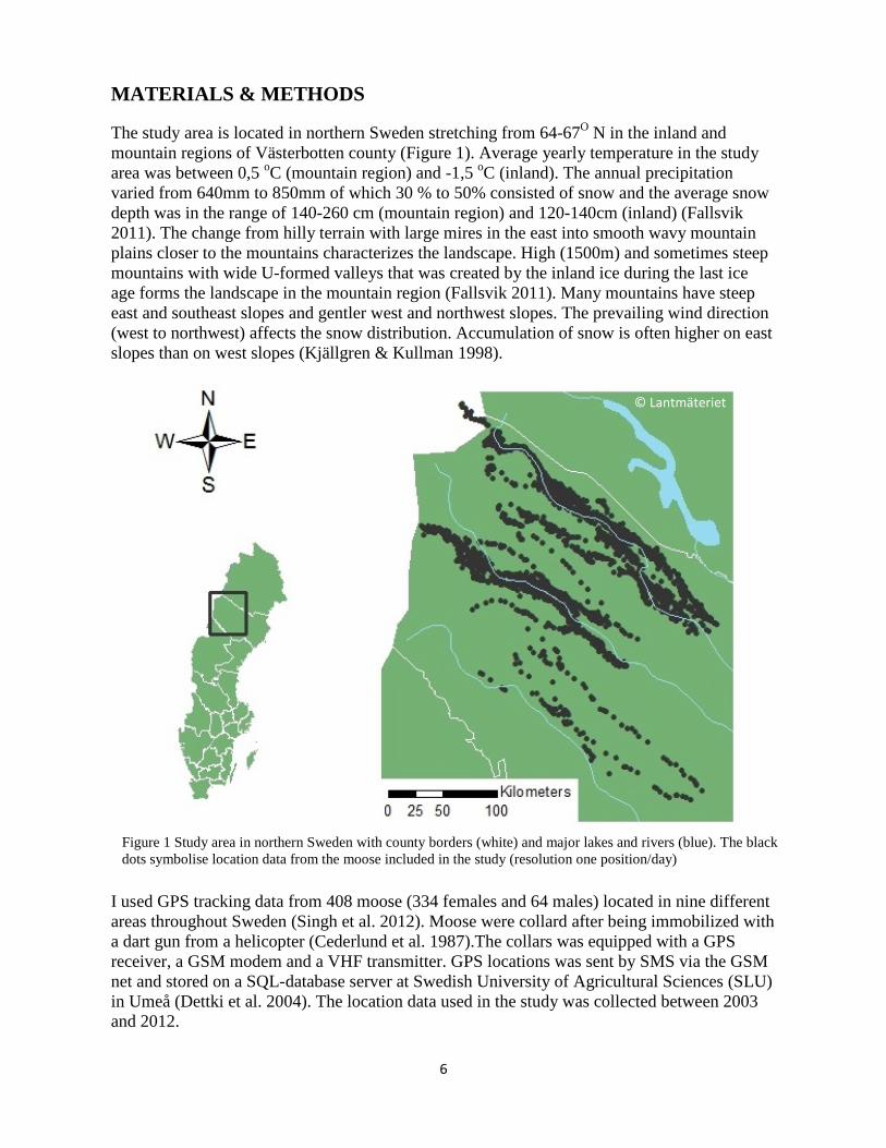
The study area is located in northern Sweden stretching from 64-67O N in the inland and mountain regions of Västerbotten county (Figure 1). Average yearly temperature in the study area was between 0,5 oC (mountain region) and -1,5 oC (inland). The annual precipitation varied from 640mm to 850mm of which 30 % to 50% consisted of snow and the average snow depth was in the range of 140-260 cm (mountain region) and 120-140cm (inland) (Fallsvik 2011). The change from hilly terrain with large mires in the east into smooth wavy mountain plains closer to the mountains characterizes the landscape. High (1500m) and sometimes steep mountains with wide U-formed valleys that was created by the inland ice during the last ice age forms the landscape in the mountain region (Fallsvik 2011). Many mountains have steep east and southeast slopes and gentler west and northwest slopes. The prevailing wind direction (west to northwest) affects the snow distribution. Accumulation of snow is often higher on east slopes than on west slopes (Kjällgren & Kullman 1998).

I used GPS tracking data from 408 moose (334 females and 64 males) located in nine different areas throughout Sweden (Singh et al. 2012). Moose were collard after being immobilized with a dart gun from a helicopter (Cederlund et al. 1987).The collars was equipped with a GPS receiver, a GSM modem and a VHF transmitter. GPS locations was sent by SMS via the GSM net and stored on a SQL-database server at Swedish University of Agricultural Sciences (SLU) in Umeå (Dettki et al. 2004). The location data used in the study was collected between 2003 and 2012.

Figure 1 Study area in northern Sweden with county borders (white) and major lakes and rivers (blue). The black dots symbolise location data from the moose included in the study (resolution one position/day)

© Lantmäteriet

7

In order to conduct the analysis all data was converted into moose-years with start date on March 21, when moose is located in its winter range. To be certain to include both summer and winter migration paths within the moose-year individual moose with a minimum of 330 days of data were selected. A full year (365 days) of data was not needed since moose spends more than one month at their winter home range (Singh et al. 2012).

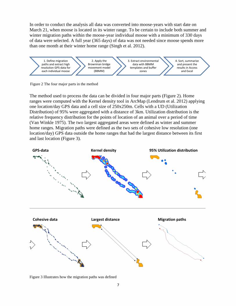
The method used to process the data can be divided in four major parts (Figure 2). Home ranges were computed with the Kernel density tool in ArcMap (Lendrum et al. 2012) applying one location/day GPS data and a cell size of 250x250m. Cells with a UD (Utilization Distribution) of 95% were aggregated with a distance of 3km. Utilization distribution is the relative frequency distribution for the points of location of an animal over a period of time (Van Winkle 1975). The two largest aggregated areas were defined as winter and summer home ranges. Migration paths were defined as the two sets of cohesive low resolution (one location/day) GPS data outside the home ranges that had the largest distance between its first and last location (Figure 3).

Figure 3 Illustrates how the migration paths was defined

1. Define migration paths and extract high resolution GPS-data for each individual moose

3. Extract environmental data with BBMM

templates and buffer zones

4. Sort, summarize and present the results in Access

and Excel

2. Apply the Browninan bridge movement model

(BBMM)

Figure 2 The four major parts in the method

GPS-data Kernel density 95% Utilization distribution

Cohesive data Largest distance Migration paths

8

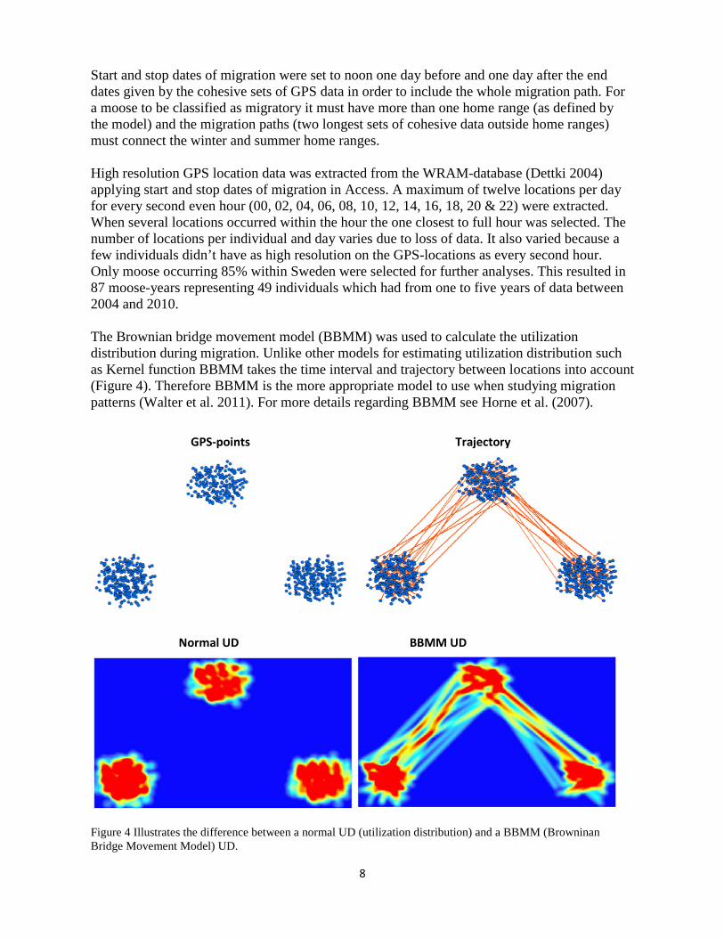
Start and stop dates of migration were set to noon one day before and one day after the end dates given by the cohesive sets of GPS data in order to include the whole migration path. For a moose to be classified as migratory it must have more than one home range (as defined by the model) and the migration paths (two longest sets of cohesive data outside home ranges) must connect the winter and summer home ranges. High resolution GPS location data was extracted from the WRAM-database (Dettki 2004) applying start and stop dates of migration in Access. A maximum of twelve locations per day for every second even hour (00, 02, 04, 06, 08, 10, 12, 14, 16, 18, 20 & 22) were extracted. When several locations occurred within the hour the one closest to full hour was selected. The number of locations per individual and day varies due to loss of data. It also varied because a few individuals didn’t have as high resolution on the GPS-locations as every second hour. Only moose occurring 85% within Sweden were selected for further analyses. This resulted in 87 moose-years representing 49 individuals which had from one to five years of data between 2004 and 2010. The Brownian bridge movement model (BBMM) was used to calculate the utilization distribution during migration. Unlike other models for estimating utilization distribution such as Kernel function BBMM takes the time interval and trajectory between locations into account (Figure 4). Therefore BBMM is the more appropriate model to use when studying migration patterns (Walter et al. 2011). For more details regarding BBMM see Horne et al. (2007).

Figure 4 Illustrates the difference between a normal UD (utilization distribution) and a BBMM (Browninan Bridge Movement Model) UD.

GPS-points Trajectory

Normal UD BBMM UD

9

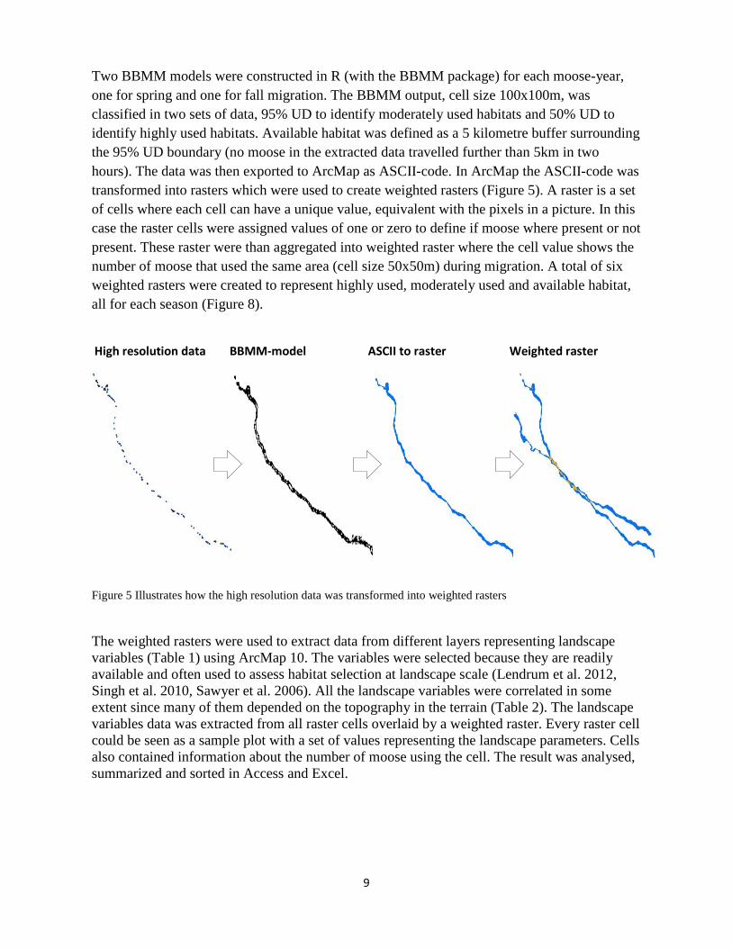
Two BBMM models were constructed in R (with the BBMM package) for each moose-year, one for spring and one for fall migration. The BBMM output, cell size 100x100m, was classified in two sets of data, 95% UD to identify moderately used habitats and 50% UD to identify highly used habitats. Available habitat was defined as a 5 kilometre buffer surrounding the 95% UD boundary (no moose in the extracted data travelled further than 5km in two hours). The data was then exported to ArcMap as ASCII-code. In ArcMap the ASCII-code was transformed into rasters which were used to create weighted rasters (Figure 5). A raster is a set of cells where each cell can have a unique value, equivalent with the pixels in a picture. In this case the raster cells were assigned values of one or zero to define if moose where present or not present. These raster were than aggregated into weighted raster where the cell value shows the number of moose that used the same area (cell size 50x50m) during migration. A total of six weighted rasters were created to represent highly used, moderately used and available habitat, all for each season (Figure 8).

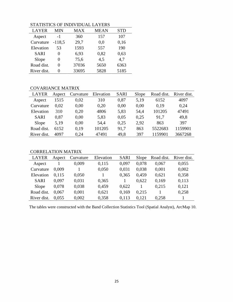
The weighted rasters were used to extract data from different layers representing landscape variables (Table 1) using ArcMap 10. The variables were selected because they are readily available and often used to assess habitat selection at landscape scale (Lendrum et al. 2012, Singh et al. 2010, Sawyer et al. 2006). All the landscape variables were correlated in some extent since many of them depended on the topography in the terrain (Table 2). The landscape variables data was extracted from all raster cells overlaid by a weighted raster. Every raster cell could be seen as a sample plot with a set of values representing the landscape parameters. Cells also contained information about the number of moose using the cell. The result was analysed, summarized and sorted in Access and Excel.

Figure 5 Illustrates how the high resolution data was transformed into weighted rasters

High resolution data BBMM-model ASCII to raster Weighted raster

10

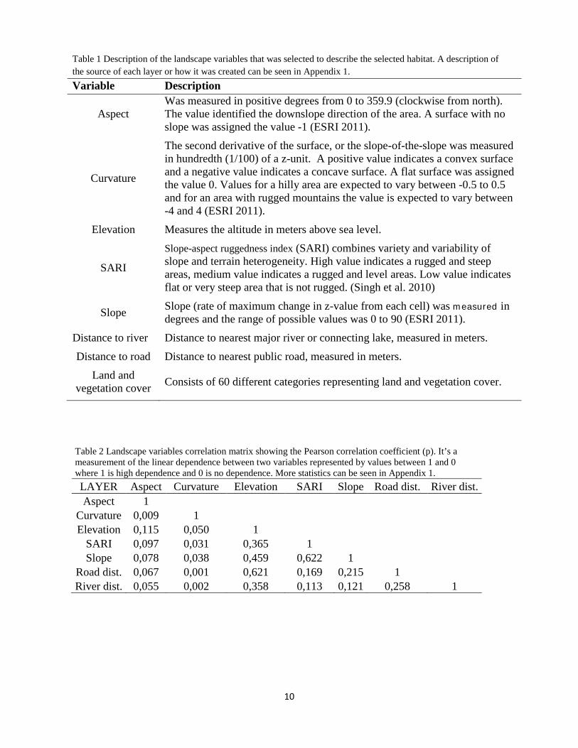
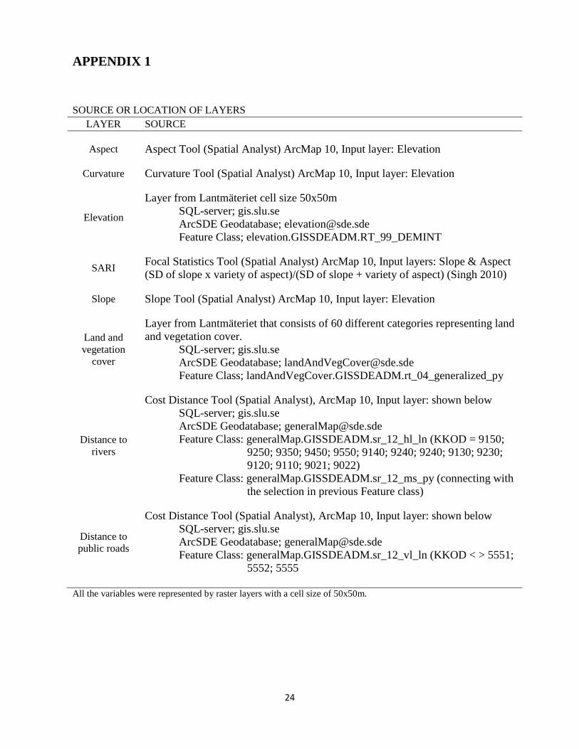
Table 1 Description of the landscape variables that was selected to describe the selected habitat. A description of the source of each layer or how it was created can be seen in Appendix 1. Variable Description

Aspect Was measured in positive degrees from 0 to 359.9 (clockwise from north). The value identified the downslope direction of the area. A surface with no slope was assigned the value -1 (ESRI 2011).

Curvature

The second derivative of the surface, or the slope-of-the-slope was measured in hundredth (1/100) of a z-unit. A positive value indicates a convex surface and a negative value indicates a concave surface. A flat surface was assigned the value 0. Values for a hilly area are expected to vary between -0.5 to 0.5 and for an area with rugged mountains the value is expected to vary between -4 and 4 (ESRI 2011).

Elevation Measures the altitude in meters above sea level.

SARI

Slope-aspect ruggedness index (SARI) combines variety and variability of slope and terrain heterogeneity. High value indicates a rugged and steep areas, medium value indicates a rugged and level areas. Low value indicates flat or very steep area that is not rugged. (Singh et al. 2010)

Slope Slope (rate of maximum change in z-value from each cell) was measured in degrees and the range of possible values was 0 to 90 (ESRI 2011).

Distance to river Distance to nearest major river or connecting lake, measured in meters.

Distance to road Distance to nearest public road, measured in meters.

Land and vegetation cover Consists of 60 different categories representing land and vegetation cover.

Table 2 Landscape variables correlation matrix showing the Pearson correlation coefficient (p). It’s a measurement of the linear dependence between two variables represented by values between 1 and 0 where 1 is high dependence and 0 is no dependence. More statistics can be seen in Appendix 1. LAYER Aspect Curvature Elevation SARI Slope Road dist. River dist. Aspect 1

Curvature 0,009 1 Elevation 0,115 0,050 1

SARI 0,097 0,031 0,365 1 Slope 0,078 0,038 0,459 0,622 1

Road dist. 0,067 0,001 0,621 0,169 0,215 1 River dist. 0,055 0,002 0,358 0,113 0,121 0,258 1

11

RESULTS

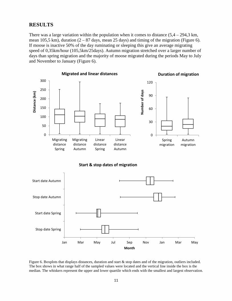
There was a large variation within the population when it comes to distance (5,4 – 294,3 km, mean 105,5 km), duration (2 – 87 days, mean 25 days) and timing of the migration (Figure 6). If moose is inactive 50% of the day ruminating or sleeping this give an average migrating speed of 0,35km/hour (105,5km/25days). Autumn migration stretched over a larger number of days than spring migration and the majority of moose migrated during the periods May to July and November to January (Figure 6).

Figure 6. Boxplots that displays distances, duration and start & stop dates and of the migration, outliers included. The box shows in what range half of the sampled values were located and the vertical line inside the box is the median. The whiskers represent the upper and lower quartile which ends with the smallest and largest observation.

0

50

100

150

200

250

300

MigratingdistanceSpring

MigratingdistanceAutumn

LineardistanceSpring

LineardistanceAutumn

Dist

ance

(km

)

Migrated and linear distances

0

30

60

90

120

Springmigration

Autumnmigration

Num

ber o

f day

s

Duration of migration

Jan Mar May Jul Sep Nov Jan Mar May

Stop date Spring

Start date Spring

Stop date Autumn

Start date Autumn

Month

Start & stop dates of migration

12

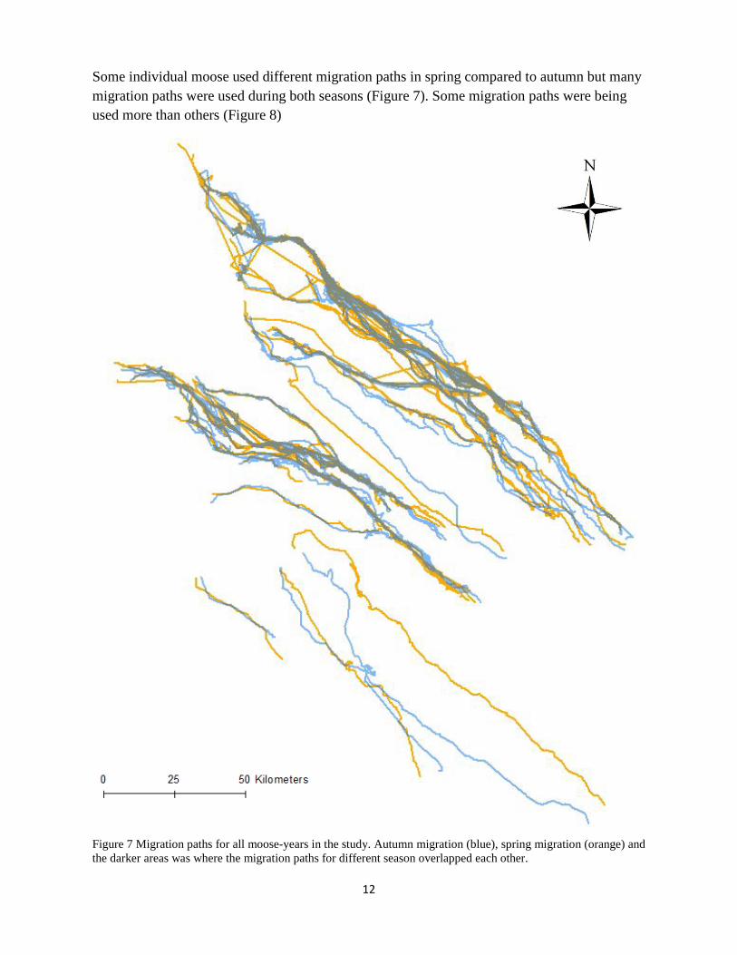
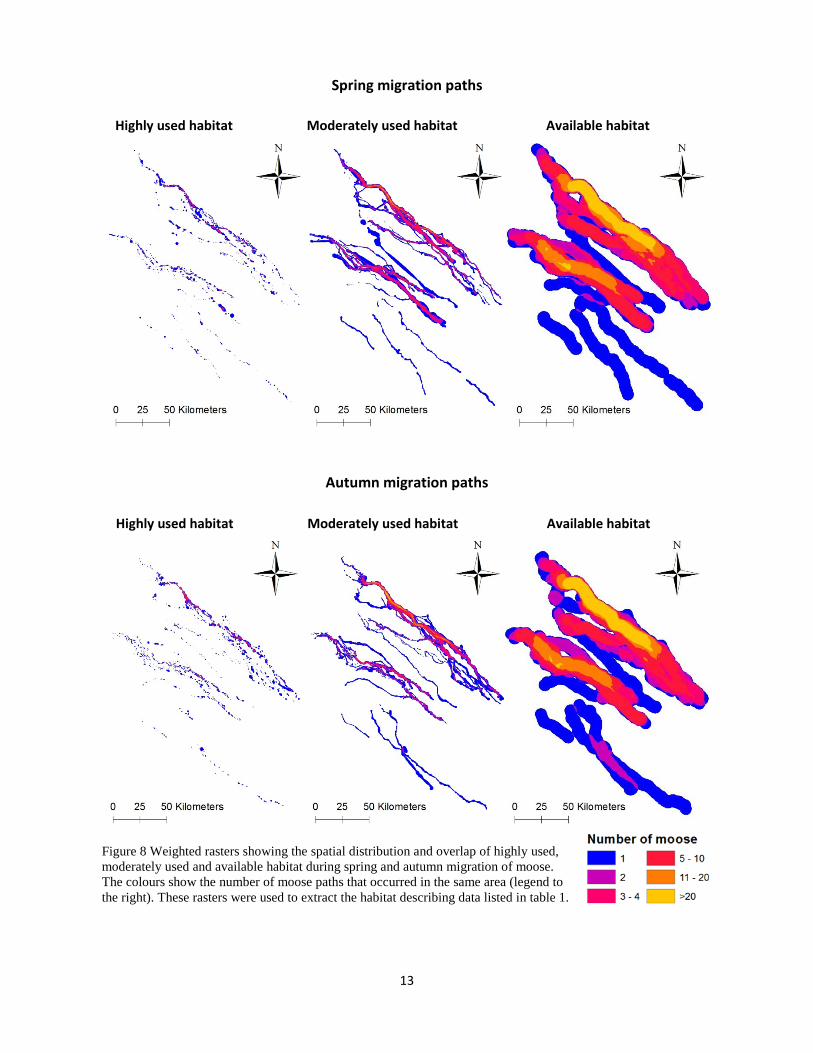
Some individual moose used different migration paths in spring compared to autumn but many migration paths were used during both seasons (Figure 7). Some migration paths were being used more than others (Figure 8)

Figure 7 Migration paths for all moose-years in the study. Autumn migration (blue), spring migration (orange) and the darker areas was where the migration paths for different season overlapped each other.

13

Spring migration paths

Autumn migration paths

Figure 8 Weighted rasters showing the spatial distribution and overlap of highly used, moderately used and available habitat during spring and autumn migration of moose. The colours show the number of moose paths that occurred in the same area (legend to the right). These rasters were used to extract the habitat describing data listed in table 1.

Highly used habitat Moderately used habitat Available habitat

Highly used habitat Moderately used habitat Available habitat

14

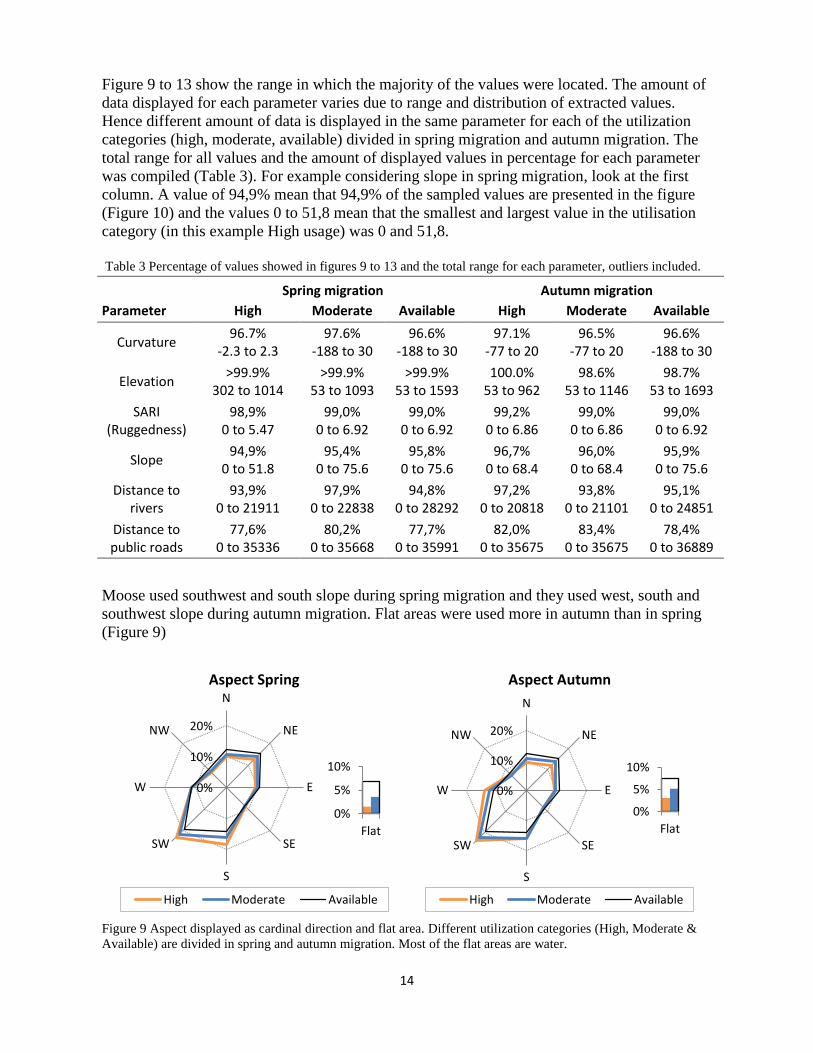
Figure 9 to 13 show the range in which the majority of the values were located. The amount of data displayed for each parameter varies due to range and distribution of extracted values. Hence different amount of data is displayed in the same parameter for each of the utilization categories (high, moderate, available) divided in spring migration and autumn migration. The total range for all values and the amount of displayed values in percentage for each parameter was compiled (Table 3). For example considering slope in spring migration, look at the first column. A value of 94,9% mean that 94,9% of the sampled values are presented in the figure (Figure 10) and the values 0 to 51,8 mean that the smallest and largest value in the utilisation category (in this example High usage) was 0 and 51,8. Table 3 Percentage of values showed in figures 9 to 13 and the total range for each parameter, outliers included.

Moose used southwest and south slope during spring migration and they used west, south and southwest slope during autumn migration. Flat areas were used more in autumn than in spring (Figure 9)

Figure 9 Aspect displayed as cardinal direction and flat area. Different utilization categories (High, Moderate & Available) are divided in spring and autumn migration. Most of the flat areas are water.

Spring migration Autumn migration Parameter High Moderate Available High Moderate Available

Curvature 96.7% 97.6% 96.6% 97.1% 96.5% 96.6% -2.3 to 2.3 -188 to 30 -188 to 30 -77 to 20 -77 to 20 -188 to 30

Elevation >99.9% >99.9% >99.9% 100.0% 98.6% 98.7% 302 to 1014 53 to 1093 53 to 1593 53 to 962 53 to 1146 53 to 1693

SARI (Ruggedness)

98,9% 99,0% 99,0% 99,2% 99,0% 99,0% 0 to 5.47 0 to 6.92 0 to 6.92 0 to 6.86 0 to 6.86 0 to 6.92

Slope 94,9% 95,4% 95,8% 96,7% 96,0% 95,9% 0 to 51.8 0 to 75.6 0 to 75.6 0 to 68.4 0 to 68.4 0 to 75.6

Distance to rivers

93,9% 97,9% 94,8% 97,2% 93,8% 95,1% 0 to 21911 0 to 22838 0 to 28292 0 to 20818 0 to 21101 0 to 24851

Distance to public roads

77,6% 80,2% 77,7% 82,0% 83,4% 78,4% 0 to 35336 0 to 35668 0 to 35991 0 to 35675 0 to 35675 0 to 36889

0%

10%

20%

N

NE

E

SE

S

SW

W

NW

Aspect Spring

High Moderate Available

0%

5%

10%

Flat

0%

10%

20%

N

NE

E

SE

S

SW

W

NW

Aspect Autumn

High Moderate Available

0%

5%

10%

Flat

15

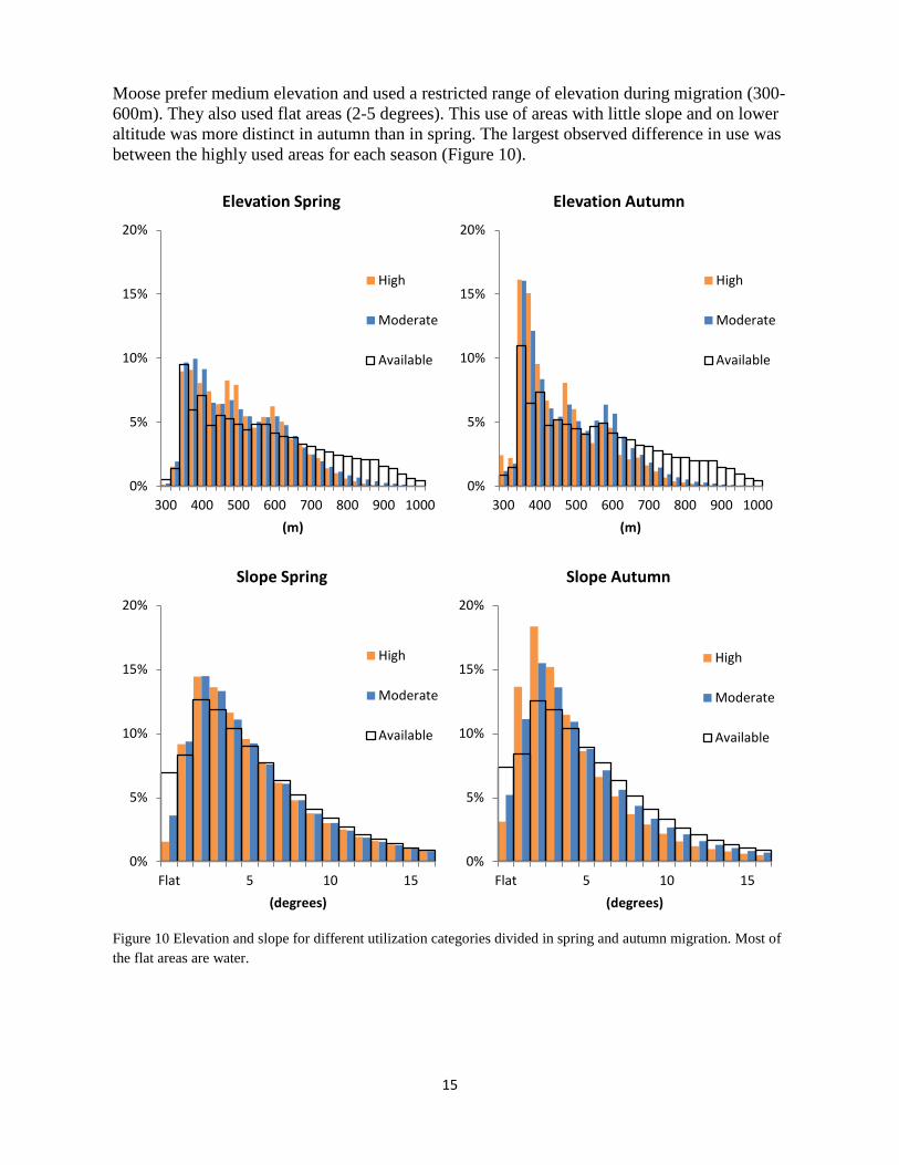
Moose prefer medium elevation and used a restricted range of elevation during migration (300-600m). They also used flat areas (2-5 degrees). This use of areas with little slope and on lower altitude was more distinct in autumn than in spring. The largest observed difference in use was between the highly used areas for each season (Figure 10).

Figure 10 Elevation and slope for different utilization categories divided in spring and autumn migration. Most of the flat areas are water.

0%

5%

10%

15%

20%

300 400 500 600 700 800 900 1000(m)

Elevation Spring

High

Moderate

Available

0%

5%

10%

15%

20%

300 400 500 600 700 800 900 1000(m)

Elevation Autumn

High

Moderate

Available

0%

5%

10%

15%

20%

Flat 5 10 15(degrees)

Slope Spring

High

Moderate

Available

0%

5%

10%

15%

20%

Flat 5 10 15(degrees)

Slope Autumn

High

Moderate

Available

16

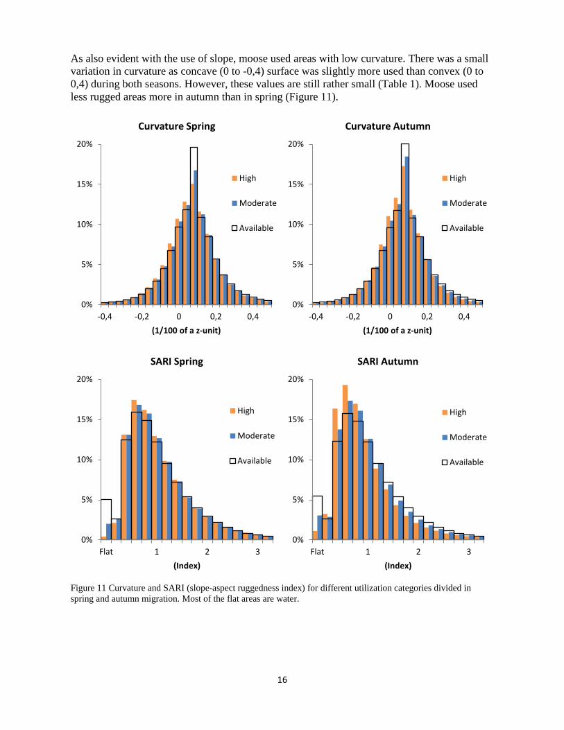
As also evident with the use of slope, moose used areas with low curvature. There was a small variation in curvature as concave (0 to -0,4) surface was slightly more used than convex (0 to 0,4) during both seasons. However, these values are still rather small (Table 1). Moose used less rugged areas more in autumn than in spring (Figure 11).

Figure 11 Curvature and SARI (slope-aspect ruggedness index) for different utilization categories divided in spring and autumn migration. Most of the flat areas are water.

0%

5%

10%

15%

20%

-0,4 -0,2 0 0,2 0,4(1/100 of a z-unit)

Curvature Spring

High

Moderate

Available

0%

5%

10%

15%

20%

-0,4 -0,2 0 0,2 0,4(1/100 of a z-unit)

Curvature Autumn

High

Moderate

Available

0%

5%

10%

15%

20%

Flat 1 2 3(Index)

SARI Autumn

High

Moderate

Available

0%

5%

10%

15%

20%

Flat 1 2 3(Index)

SARI Spring

High

Moderate

Available

17

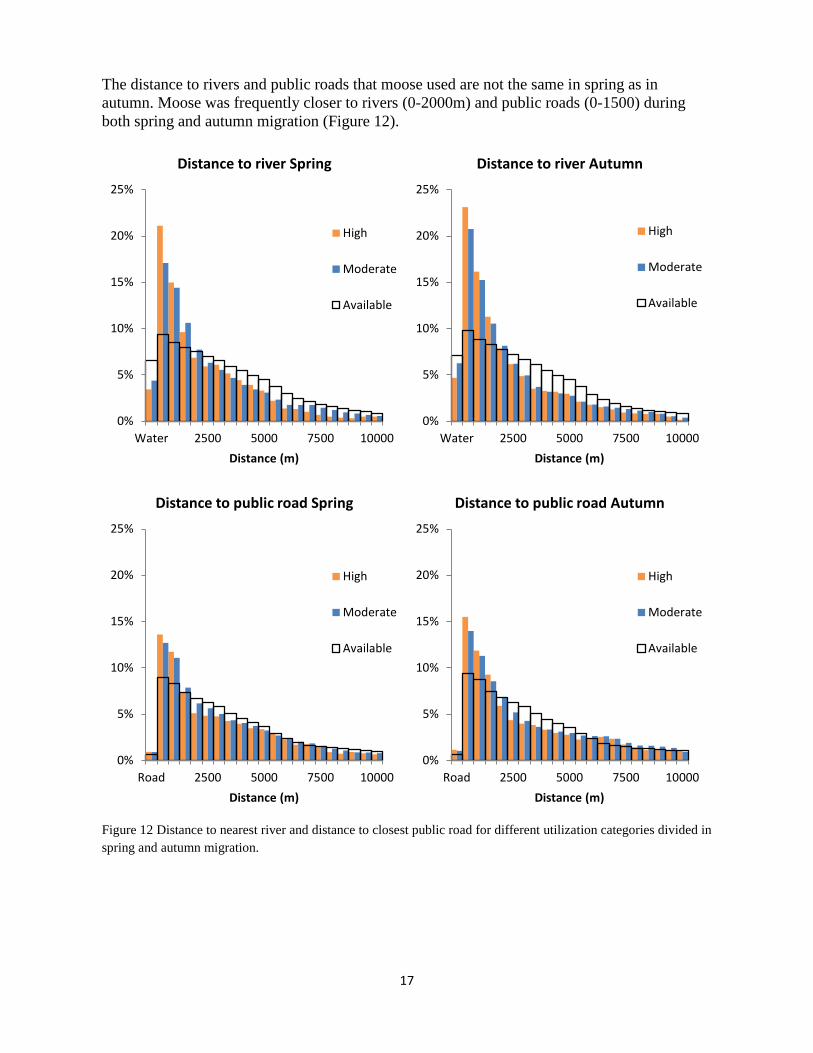
The distance to rivers and public roads that moose used are not the same in spring as in autumn. Moose was frequently closer to rivers (0-2000m) and public roads (0-1500) during both spring and autumn migration (Figure 12).

Figure 12 Distance to nearest river and distance to closest public road for different utilization categories divided in spring and autumn migration.

0%

5%

10%

15%

20%

25%

Water 2500 5000 7500 10000Distance (m)

Distance to river Spring

High

Moderate

Available

0%

5%

10%

15%

20%

25%

Water 2500 5000 7500 10000Distance (m)

Distance to river Autumn

High

Moderate

Available

0%

5%

10%

15%

20%

25%

Road 2500 5000 7500 10000Distance (m)

Distance to public road Spring

High

Moderate

Available

0%

5%

10%

15%

20%

25%

Road 2500 5000 7500 10000Distance (m)

Distance to public road Autumn

High

Moderate

Available

18

Open areas like clear cuts, young forest, heathland and mire were used more during autumn migration while coniferous forest, not located on lichen fields, were used during spring migrations. Grasslands were not used and lakes, ponds and rivers along with coniferous forest, on lichen fields were more used in autumn. Deciduous forests were used during both seasons (Figure 13).

Figure 13 Land and vegetation cover for different utilization categories divided in spring and autumn migration.

0%

5%

10%

15%

20%

25%Land & vegetation cover Spring

High

Moderate

Available

0%

5%

10%

15%

20%

25%Land & vegetation cover Autumn

High

Moderate

Available

19

DISCUSSION

I show that moose used some environmental attributes more than others during migration and that there are observed differences in habitat use between seasons and utilization categories. There are both spatial and habitat differences in selection between spring and autumn migration, however many migration paths are being used during both seasons. Moose generally used level areas in southwest slope on a low altitude not far from rivers and roads. Open areas is used more during autumn migration while coniferous forest is used in spring and deciduous forests is used both seasons. This is expected since moose use landscapes with a lot of wetland, lakes and young tree stands. They prefer dense undergrowth of deciduous trees and shrubs as forage but pine is also an important food source, especially during winters (Maier et al. 2005, Jensen 2004). Moose are known to use habitat close to major rivers (Safronov 2009, Maier et al. 2005, Ballard et al. 1991, Boyce 1991) and the population in this study seems to use that kind of habitat when migrating. Rivers and roads often go alongside each other in the study area and moose was located in closer proximity to rivers than to roads. This suggests that moose prefer to be close to rivers while trying to avoid roads. Lendrum et al. (2012) show that deer tries to avoid roads and human disturbance during migration without altering their routes substantially. Deer have a high fidelity towards their migration routes and assumed it’s hard to avoid disturbed area they might choose to pass swiftly through them (Lendrum et al. 2012). Moose generally show fidelity to their home ranges and calving sites (van Beest et al. 2010, Tremblay et al. 2007, Sweanor & Sandegren 1989) and may therefore respond in the same way as the deer. The use of low elevation, slope and ruggedness (SARI) is more distinct in autumn than in spring. Additionally lakes, ponds and rivers represent a larger part of the land & vegetation cover in autumn than in spring. This suggests that habitat use is more tied to river valleys during autumn migration compared to spring migration. Moose also use areas in a southwest slope during migration which can have many explanations. Snow melts earlier on southern slopes than on northern slopes (Morén & Perttu 1994). West slopes have less snow than east slopes due to wind direction and steepness (Kjällgren & Kullman 1998). The vegetation cover varies between different aspects (Holland & Steyn 1975) with more broadleaf trees in south slopes (Åström 2006). There was a large variation within the population when it comes to distance, duration and timing of the migration (Figure 5) which is consistent with previous research. Both Singh et al. (2012) and Ballard et al. (1991) observed large variations within populations regarding these variables. According to this study the migrating distance varies from 5,4 to 294,3 km with an average of 105,5 km. Corresponding results in Singh et al. (2012) is a variation from 5,4 to 217,0 km with an average of 103,1 km. When it comes to timing and duration of migration the differences are more substantial. The duration period presented by Singh et al. (2012) is one to two weeks shorter than the results of this study suggests. Singh et al. (2012) also show that the duration of autumn migration is shorter than in spring migration which contradicts the results of this study. These differences are probably due to the fact that different methods were used to define and extract the migration paths.

20

According to Bolger et al. (2008) migration routes used by ungulates often varies from season to season and some migration paths is used more than others (Sawyer et al. 2009). Figure 6 show that some individuals use different migration paths for each season. It also shows that some migration paths are used during both spring and autumn migration. The number of moose that use the same migration paths may in this case be affected by in what area most moose were collared and how many years of data each moose have. In this study the number of years for each individual moose varies from one to five. The lowest number of moose that use the same area is found in the category highly used habitat (Figure 7). This correlates with Lojander (2013) in the result that stopover site fidelity is low. Sometimes it’s unclear when a moose begin or end its migration and therefore problematic to delimit the whole migration path. The definition used in this study can possibly be improved by defining the home ranges in a different way. As they are defined now a slow starting moose may be assigned home ranges that cover some of the migration route. Perhaps it’s better to build the home ranges upon the areas with the highest kernel density instead of the largest areas with 95% kernel utilization distribution. However, the low speeds of migration observed here suggest that more precisely delineating the exact beginning and end of migration is unlikely to be really important in understanding migratory behaviour. The results may be slightly bias due the fact that some individuals are represented with more years of data than others. If the majority of moose in the study was collard in the same area the results may be affected. Furthermore, the data representing land and vegetation cover is from 2004 while the moose data is from 2004 to 2010. The change in land and vegetation cover occurring over the years is therefore not included. I show that there are differences in both spatial and habitat use for moose between seasons and different utilization categories. Some individuals select different paths in spring compared to autumn but many migration paths is being used during both seasons. Moose seems to select migration paths that results in a low cost of energy and where there is a good amount of high quality food. The results can be applied when deciding where to make wildlife passages and where to construct fences. Moose is not a threatened species but even huge population may face extinction due to habitat destruction and over harvest, like the passenger pigeon in the USA (Pollock 2003). The method applied in this study can be used on other species to determine and quantify the habitat that they use which is essential knowledge to possess when working with conservation. In order to do this high resolution GPS-data is needed which unfortunately takes much time and costs a lot of money to gather and store. Since different populations of moose have demonstrated dissimilar migratory behaviour (Singh et al. 2012, Safronov 2009) it would be interesting to analyse them in the same way as the population in this study and compare the results. Further analysis would be needed in order to understand if moose selects optimum migration routes. To do this the ratio between the different habitat variables and how they affect each other needs to be determined. If there is a road alongside a southwest slope of a river valley does moose chose the northeast slope on the other side of the valley in order to avoid the road? This is the kind of question that might be answered with further statistical analysis.

21

ACKNOWLEDGMENTS

I would like to thank my supervisor Dr. Navinder J Singh and assistant supervisor Prof. Göran Ericsson. A special thanks to Peter Lojander, my brother in arms during this thesis.

LITERATURE

Ball, J.P. & Dahlgren, J. 2002. Browsing damage on pine (Pinus sylvestris and P. contorta) by a migrating moose (Alces alces) population in winter: Relation to habitat composition and road barriers. Scandinavian Journal of Forest Research 17(5): 427-435. Ballard, W.B., Whitman, J.S. & Reed, D.J. 1991. Population dynamics of moose in south- central Alaska. Wildlife Monographs 114: 1-49. Berger, J. 2004. The last mile: How to sustain long-distance migration in mammals. Conservation Biology 18(2): 320-331. Berger, J., Cain, L.C. & Berger K.M. 2006. Connecting the dots: an invariant migration corridor links the Holocene to the present Biology Letters 2: 528-531. Bolger, D.T., Newmark, W.D., Morrison, T.A. & Doak, D.F. 2008. The need for integrative approaches to understand and conserve migratory ungulates. Ecology Letters 11: 63–77. Bowlin, M.S., Bisson, I.-A., Shamoun-Baranes, J., Reichard, J.D., Sapir, N., Marra, P.P., Kunz, T.H., Wilcove, D.S., Hedenström, A., Guglielmo, C.G., Kesson, S.A., Ramenofsky, M. & Wikelski, M. 2010. Grand challenges in migration biology. Integrative and comparative biology 50(3): 261-279. Boyce, M.S. 1991. Migration behavior and management of elk (Cervus elaphus). Applied Animal Behaviour Science 29: 239-250. Cederlund, G., Sandegren, F. & Larsson, K. 1987. Summer movements of female moose and dispersal of their offspring. The Journal of Wildlife Management 51(2): 342-352. Dettki, H., Ericsson, G. & Edenius, L. 2004. Real-time moose tracking: An internet based mapping application using GPS/GSM-collars in Sweden. Alces 40: 13-21. Dingle, H. & Drake, V.A. 2007. What is migration?. Bioscience 57(2): 113-121. ESRI (Environmental Systems Resource Institute). 2011. ArcMap 10. ESRI, Redlands, California. Fallsvik, J. 2011. Översiktlig klimat- och sårbarhetsanalys – Naturolyckor. Rapport SGI Diarienummer: 2-1005-0372. Linköping. Grovenburg, T.W., Jacques, C.N., Klaver, R.W., DePerno, C.S., Brinkman, T.J., Swanson, C.C. & Jenks, J.A. 2011. Influence of landscape characteristics on migration strategies of white-tailed deer. Journal of Mammalogy 92(3): 534-543. Harris, G., Thirgood, S., Hopcraft, J.G.C., Cromsigt, J.P.G.M. & Berger, J. 2009. Global decline in aggregated migrations of large terrestrial mammals. Endangered Species Research 7: 55-76. Hebblewhite, M., Merrill, E.H., Morgantini, L.E., White, C.A., Allen, J.R., Bruns, E., Thurston, L. & Hurd, T.E. 2006. Is the migratory behavior of Montane elk herds in peril? The case of Alberta's Ya Ha Tinda elk herd. Wildlife Society Bulletin 34(5): 1280-1294. Hebblewhite, M., Merrill, E.H. & McDermid, G. 2008. A multi-scale test of the forage maturation hypothesis in a partially migratory ungulate population. Ecological Monographs, 78(2): 141-166. Holland, P.G. & Steyn, D.G. 1975. Responses to latitudinal variations in slope angle and aspect. Journal of Biogeography 2(3): 179-183.

22

Horne, J.S., Garton, E.O., Krone, S.M. & Lewis, J.S. 2007. Analyzing animal movements using Brownian bridges. Ecology 88(9): 2354-2363. Houston, A.I., McNamara, J.M. & Hutchinson, J.M.C. 1993. General results concerning the trade-off between gaining energy and avoiding predation. Philosophical Transactions: Biological Sciences 341(1298): 375-397. Jensen, B. 2004. Nordens pattedyr 2nd edition. Gyldendalske boghandel. Köpenhamn. Kjällgren, L. & Kullman, L. 1998. Spatial patterns and structure of the mountain birch tree- limit in the southern Swedish Scandes - a regional perspective. Geografiska Annaler 80A(1): 1-16. Lavsund, S., Nygren, T. & Solberg, E.J. 2003. Status of moose populations and challenges to moose management in Fennoscandia. Alces 39: 109-130. Lendrum, P.E., Anderson, C.R.JR, Long, R.A., Kie, J.G. & Bowyer, R.T. (2012). Habitat selection by mule deer during migration: effects of landscape structure and natural-gas development. Ecosphere 3(9): 1-19. Lojander, P. 2013. Site fidelity of a migratory species of the northern hemisphere. Master thesis, Swedish University of Agricultural Sciences. Lundberg, J. & Moberg, F. 2003. Mobile link organisms and ecosystem functioning: implications for ecosystem resilience and management. Ecosystems 6(1): 87-98. Maier, J.A.K., Ver Hoef, J.M., McGuire, A.D., Bowyer, R.T., Saperstein, L. & Maier, H.A. 2005. Distribution and density of moose in relation to landscape characteristics: effects of scale. Canadian journal of forest research 35(9): 2233-2243. Morén, A.-S. & Perttu, K.L. 1994. Regional temperature and radiation indices and their adjustment to horizontal and inclined forest land. Studia Forestalia Suecica 194: 1-19. Neumann, W., Ericsson, G., Dettki, H., Bunnefeld, N., Keuler, N.S., Helmers, D.P. & Radeloff, V.C. 2011. Difference in spatiotemporal patterns of wildlife road-crossings and wildlife-vehicle collisions. Biological Conservation 145: 70-78. Pollock, C. 2003. The passenger pigeon. Journal of Avian Medicine and Surgery 17(2): 97-98. Safronov, V.M. 2009. Regional populations and migration of moose in northern yakutia, Russia. Alces 45: 17-20. Sawyer, H., Nielson, R.M., Lindzey, F. & McDonald, L.L. 2006. Winter habitat selection of mule deer before and during development of a natural gas field. The Journal of Wildlife Management 70(2): 396-403. Sawyer, H., Kauffman, M.J., Nielson, R.M. & Horne, J.S. 2009. Identifying and prioritizing ungulate migration routes for landscape-level conservation. Ecological Applications, 19(8): 2016–2025. Sawyer, H., Kauffman, M.J., Middleton, A.D., Morrison, T.A., Nielson, R.M. & Wyckoff, T.B. 2012 .A framework for understanding semi-permeable barrier effects on migratory ungulates. Journal of Applied Ecology 49(6): 1-11 Singh, N.J., Yoccoz, N.G., Lecomte, N., Côté, S.D. & Fox, J.L. 2010. Scale and selection of habitat and resources: Tibetan argali (Ovis ammon hodgsoni) in high-altitude rangelands. Canadian Journal of Zoology 88(5): 436-447. Singh, N.J. & Milner-Gulland, E.J. 2011. Conserving a moving target: planning protection for a migratory species as its distribution changes. Journal of Applied Ecology 48: 35-46. Singh, N.J., Börger, L., Dettki, H., Bunnefeld, N. & Ericsson, G. 2012. From migration to nomadism: movement variability in a northern ungulate across its latitudinal range. Ecological Applications 22(7): 2007-2020. Sweanor, P.Y. & Sandegren, F. 1988. Migratory behavior of related moose. Holarctic Ecology 11(3): 190-193.

23

Sweanor, P.Y. & Sandegren, F. 1989. Winter-range philopatry of seasonally migratory moose. Journal of Applied Ecology 26(1): 25-33. Tremblay, J.-P., Solberg, E.J., Saether, B.-E. & Heim, M. 2007. Calving site fidelity in moose (Alces alces) in the absence of large carnivores. Canadian Journal of Zoology 85(8): 902- 908. Walter, W.D., Fischer, J.W., Baruch-Mordo, S. & VerCauteren, K.C. 2011. What is the proper method to delineate home range of an animal using today’s advanced GPS telemetry systems: the initial step, in Krejcar, O. Modern Telemetry. InTech. Rijeka. 249-268. van Beest, F.M., Mysterud, A., Loe, L.E. & Milner, J.M. 2010. Forage quantity, quality and depletion as scale dependent mechanisms driving habitat selection of a larger browsing herbivore. Journal of Animal Ecology 79(4): 910-922. Van Winkle, W. 1975. Comparison of several probabilistic home-range models .The Journal of Wildlife Management. 39(1): 118-123. Wilcove, D.S. & Wikelski, M. 2008. Going, going, gone: Is animal migration disappearing?. PLoS Biology 6(7): 1361-1364. Åström, M. 2006. Aspects of heterogeneity: effects of clear-cutting and post-harvest extraction of bioenergy on plants in boreal forests. Doctoral Dissertation. ISBN: 91-7264-192-4

24

APPENDIX 1

SOURCE OR LOCATION OF LAYERS LAYER SOURCE

Aspect Aspect Tool (Spatial Analyst) ArcMap 10, Input layer: Elevation

Curvature Curvature Tool (Spatial Analyst) ArcMap 10, Input layer: Elevation

Elevation

Layer from Lantmäteriet cell size 50x50m SQL-server; gis.slu.se ArcSDE Geodatabase; elevation@sde.sde Feature Class; elevation.GISSDEADM.RT_99_DEMINT

SARI Focal Statistics Tool (Spatial Analyst) ArcMap 10, Input layers: Slope & Aspect (SD of slope x variety of aspect)/(SD of slope + variety of aspect) (Singh 2010)

Slope Slope Tool (Spatial Analyst) ArcMap 10, Input layer: Elevation

Land and vegetation

cover

Layer from Lantmäteriet that consists of 60 different categories representing land and vegetation cover.

SQL-server; gis.slu.se ArcSDE Geodatabase; landAndVegCover@sde.sde Feature Class; landAndVegCover.GISSDEADM.rt_04_generalized_py

Distance to rivers

Cost Distance Tool (Spatial Analyst), ArcMap 10, Input layer: shown below SQL-server; gis.slu.se ArcSDE Geodatabase; generalMap@sde.sde Feature Class: generalMap.GISSDEADM.sr_12_hl_ln (KKOD = 9150;

9250; 9350; 9450; 9550; 9140; 9240; 9240; 9130; 9230; 9120; 9110; 9021; 9022)

Feature Class: generalMap.GISSDEADM.sr_12_ms_py (connecting with the selection in previous Feature class)

Distance to public roads

Cost Distance Tool (Spatial Analyst), ArcMap 10, Input layer: shown below SQL-server; gis.slu.se ArcSDE Geodatabase; generalMap@sde.sde Feature Class: generalMap.GISSDEADM.sr_12_vl_ln (KKOD < > 5551;

5552; 5555

All the variables were represented by raster layers with a cell size of 50x50m.

25

STATISTICS OF INDIVIDUAL LAYERS LAYER MIN MAX MEAN STD

Aspect -1 360 157 107 Curvature -118,5 29,7 0,0 0,16 Elevation 53 1593 557 190 SARI 0 6,93 0,82 0,63 Slope 0 75,6 4,5 4,7 Road dist. 0 37036 5650 6363 River dist. 0 33695 5828 5185

COVARIANCE MATRIX

LAYER Aspect Curvature Elevation SARI Slope Road dist. River dist. Aspect 1515 0,02 310 0,87 5,19 6152 4097

Curvature 0,02 0,00 0,20 0,00 0,00 0,19 0,24 Elevation 310 0,20 4806 5,83 54,4 101205 47491

SARI 0,87 0,00 5,83 0,05 0,25 91,7 49,8 Slope 5,19 0,00 54,4 0,25 2,92 863 397

Road dist. 6152 0,19 101205 91,7 863 5522683 1159901 River dist. 4097 0,24 47491 49,8 397 1159901 3667268

CORRELATION MATRIX

LAYER Aspect Curvature Elevation SARI Slope Road dist. River dist. Aspect 1 0,009 0,115 0,097 0,078 0,067 0,055

Curvature 0,009 1 0,050 0,031 0,038 0,001 0,002 Elevation 0,115 0,050 1 0,365 0,459 0,621 0,358

SARI 0,097 0,031 0,365 1 0,622 0,169 0,113 Slope 0,078 0,038 0,459 0,622 1 0,215 0,121

Road dist. 0,067 0,001 0,621 0,169 0,215 1 0,258 River dist. 0,055 0,002 0,358 0,113 0,121 0,258 1

The tables were constructed with the Band Collection Statistics Tool (Spatial Analyst), ArcMap 10.

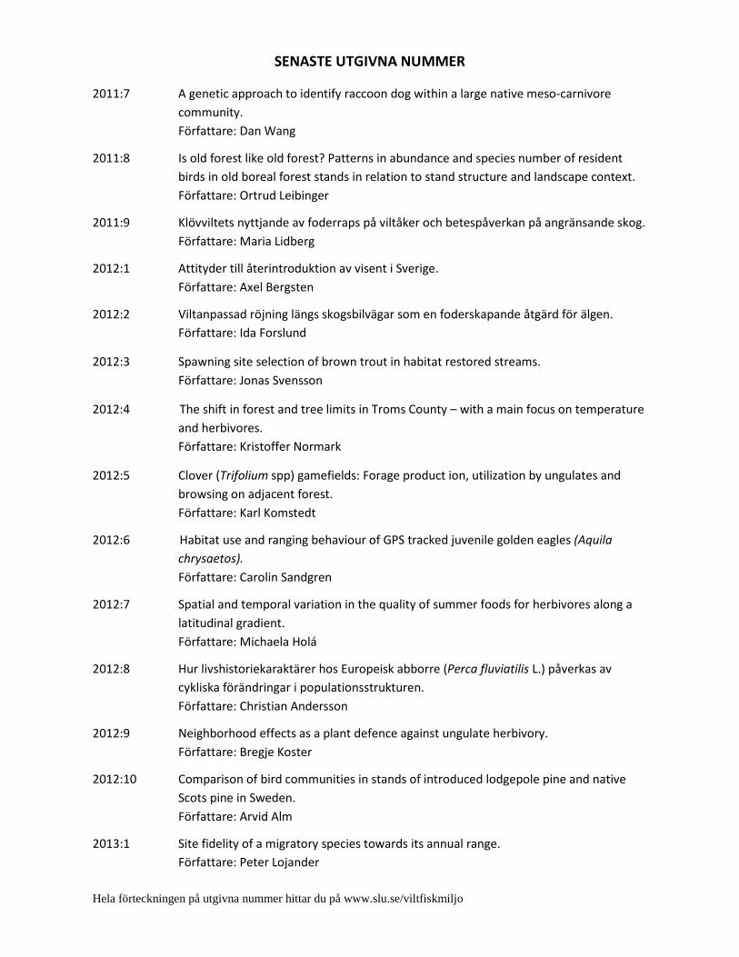
SENASTE UTGIVNA NUMMER

2011:7 A genetic approach to identify raccoon dog within a large native meso-carnivore community. Författare: Dan Wang

2011:8 Is old forest like old forest? Patterns in abundance and species number of resident birds in old boreal forest stands in relation to stand structure and landscape context. Författare: Ortrud Leibinger

2011:9 Klövviltets nyttjande av foderraps på viltåker och betespåverkan på angränsande skog. Författare: Maria Lidberg

2012:1 Attityder till återintroduktion av visent i Sverige. Författare: Axel Bergsten

2012:2 Viltanpassad röjning längs skogsbilvägar som en foderskapande åtgärd för älgen. Författare: Ida Forslund

2012:3 Spawning site selection of brown trout in habitat restored streams. Författare: Jonas Svensson

2012:4 The shift in forest and tree limits in Troms County – with a main focus on temperature and herbivores.

Författare: Kristoffer Normark

2012:5 Clover (Trifolium spp) gamefields: Forage product ion, utilization by ungulates and browsing on adjacent forest. Författare: Karl Komstedt

2012:6 Habitat use and ranging behaviour of GPS tracked juvenile golden eagles (Aquila chrysaetos). Författare: Carolin Sandgren

2012:7 Spatial and temporal variation in the quality of summer foods for herbivores along a latitudinal gradient. Författare: Michaela Holá

2012:8 Hur livshistoriekaraktärer hos Europeisk abborre (Perca fluviatilis L.) påverkas av cykliska förändringar i populationsstrukturen. Författare: Christian Andersson

2012:9 Neighborhood effects as a plant defence against ungulate herbivory. Författare: Bregje Koster

2012:10 Comparison of bird communities in stands of introduced lodgepole pine and native Scots pine in Sweden. Författare: Arvid Alm

2013:1 Site fidelity of a migratory species towards its annual range. Författare: Peter Lojander Hela förteckningen på utgivna nummer hittar du på www.slu.se/viltfiskmiljo