Embed Size (px)
Citation preview
University of PadovaDepartment of Information Engineering
Ph.D. course on Bioelectromagnetism and Electromagnetic CompatibilityXXI Cycle
Ph.D. Thesis
Evaluation of Uncertainty and Repeatability inMeasurement: two application studies in
Synchronization and EMC Testing
Supervisor: Ch.mo Prof. Claudio Narduzzi
Co-examiner: Dott. Ing. Alessandro Sona
Ph.D. candidate: Ing. Marco Stellini
January, 2009

Abstract
Efficient organization of measurement tasks requires the knowledge and characterization of theparameters and of the effects that may affect the measurement itself. Uncertainty analysis isan example of how measurement accuracy is often difficult to quantify. Repeatability also as-sumes a key role. This is the ability to replicate the tests and related measurements at differenttimes. The research was focused on this aspect of analysis of test repeatability. Some specificcase studies in the field of measurements relating to synchronization between network nodesand to measurements for Electromagnetic Compatibility have been considered.Synchronization between the components of a system is a particularly important requirementwhen considering distributed structures. The network nodes developed for this research arebased on both PCs with a Real Time operating system (RTAI) and Linux-based embedded sys-tems (FOX Acme Systems Board) interfaced to an auxiliary module with a field-programmablegate array (FPGA). The aim of the tests is to measure and classify the uncertainty due to jitterin the Time Stamping mechanism, and consequently to evaluate the resolution and repeatabil-ity of synchronization achieved in different traffic conditions using a standardized protocol forsynchronization (IEEE 1588-PTPd).The work in the Electromagnetic Compatibility has likewise focused on the repeatability ofmeasurements typical of some practical applications. Some experiments involving LISN cal-ibration have been carried out and some improvements are presented to reduce uncertainty.Theoretical and experimental uncertainty analysis associated with the ESD tests has been con-ducted and some possible solutions are proposed. A study on the performance of sites forradiated tests (Anechoic chambers, open-area test site) has been started using simulations andexperimental testing in order to assess the capability of different sites. Obtained results arecompared with different reference sources.Finally, the results of a research project carried out at the University of Houston for the propa-gation of electromagnetic fields are reported.

Sommario
Organizzare una efficiente campagna di misure richiede la conoscenza e la caratterizzazionedei parametri e degli effetti che possono influire sulla misura stessa. L’analisi dell’incertezza èun esempio di come l’accuratezza sia spesso difficile da quantificare. Oltre all’incertezza tut-tavia assume un ruolo chiave la ripetibilità, ovvero la possibilità di replicare il test e le relativemisure in momenti diversi. L’attività di ricerca ha riguardato proprio questo aspetto di analisidella ripetibilità dei test prendendo in considerazione alcuni casi di studio specifici sia in am-bito di Misure relative alla Sincronizzazione tra nodi di un sistema distribuito sia di Misure perla Compatibilità Elettromagnetica.La sincronizzazione è un’esigenza particolarmente sentita quando si considerano strutture dimisura distribuite. I nodi di rete sviluppati per queste ricerche sono basati sia su PC dotatidi sistema operativo Real Time (RTAI) sia su sistemi embedded Linux-based (Acme SystemsFOX Board) interfacciati ad un modulo ausiliario su cui si trova un field-programmable gatearray (FPGA). I test condotti hanno permesso di misurare e classificare l’incertezza dovutaal jitter nel meccanismo di Time Stamp, e conseguentemente di valutare la risoluzione e laripetibilità della sincronizzazione raggiunta in diverse condizioni di traffico utilizzando un pro-tocollo di sincronizzazione standardizzato secondo l’IEEE 1588 (PTPd).In ambito di compatibilità elettromagnetica, il lavoro svolto si è concentrato sull’analisi dellaripetibilità di misure tipiche di alcune applicazioni pratiche in ambito EMC. E’ stata svolta unaanalisi approfondita dei fenomeni parassiti legati alla taratura di una LISN e sono stati introdottialcuni miglioramenti costruttivi al fine di ridurre i contributi di incertezza. Si è condotta unaindagine teorico-sperimentale sull’incertezza associata alla misura di immunità con generatoredi scariche elettrostatiche e l’individuazione di possibili soluzioni. E’ stato avviato uno studiosulle prestazioni dei siti per le misure dei disturbi irradiati (camere anecoiche, open-area testsite) mediante simulazioni teoriche e prove ’in campo’ al fine di valutare i limiti di impiego deidiversi siti e comparare i risultati ottenuti con sorgenti di riferimento.Infine, vengono riportati i risultati di una ricerca svolta presso l’Università di Houston e relativaalla propagazione di campi elettromagnetici.

Contents
General Introduction 1
I Analysis of Accuracy in Time Synchronization 5
Introduction - Part I 7IEEE 1588 . . . . . . . . . . . . . . . . . . . . . . . . . . . . . . . . . . . . . . . . 9
1 Test Bed description 131.1 Timing accuracy of scheduled software tasks . . . . . . . . . . . . . . . . . . 13
1.1.1 RTAI Extension . . . . . . . . . . . . . . . . . . . . . . . . . . . . . . 151.1.2 Time response performance . . . . . . . . . . . . . . . . . . . . . . . 16
1.2 First Test Bed Implementation - PC nodes with background traffic . . . . . . . 181.3 Second Solution - Synchronization with emulated cross-traffic . . . . . . . . . 20
1.3.1 Embedded Systems . . . . . . . . . . . . . . . . . . . . . . . . . . . . 201.3.2 Test Bed . . . . . . . . . . . . . . . . . . . . . . . . . . . . . . . . . 211.3.3 Cross traffic generation . . . . . . . . . . . . . . . . . . . . . . . . . . 221.3.4 Implementation issues . . . . . . . . . . . . . . . . . . . . . . . . . . 231.3.5 Validation of the traffic generator . . . . . . . . . . . . . . . . . . . . 23
2 Synchronization Tests and Analysis 252.1 Preliminary Investigations . . . . . . . . . . . . . . . . . . . . . . . . . . . . 25
2.1.1 Single Clock Analysis . . . . . . . . . . . . . . . . . . . . . . . . . . 252.1.2 Performance limits . . . . . . . . . . . . . . . . . . . . . . . . . . . . 252.1.3 Network switch . . . . . . . . . . . . . . . . . . . . . . . . . . . . . . 272.1.4 Network traffic . . . . . . . . . . . . . . . . . . . . . . . . . . . . . . 282.1.5 Measurement Analysis . . . . . . . . . . . . . . . . . . . . . . . . . . 29
2.2 Further Generic Tests . . . . . . . . . . . . . . . . . . . . . . . . . . . . . . . 302.2.1 Synchronization analysis . . . . . . . . . . . . . . . . . . . . . . . . . 32
II Calibration and Repeatability in EMC Tests 37
Introduction - Part II 39EMI/EMC Test Lab . . . . . . . . . . . . . . . . . . . . . . . . . . . . . . . . . . . 40

viii Contents
Standards . . . . . . . . . . . . . . . . . . . . . . . . . . . . . . . . . . . . . . . . 41
3 Field propagation in SA-Chamber 433.1 Chamber Factors . . . . . . . . . . . . . . . . . . . . . . . . . . . . . . . . . 44
3.2 Characterization of the Investigated Test Site . . . . . . . . . . . . . . . . . . 45
3.2.1 NSA Characterization . . . . . . . . . . . . . . . . . . . . . . . . . . 46
3.2.2 CF Characterization . . . . . . . . . . . . . . . . . . . . . . . . . . . 46
3.2.3 OATS Characterization . . . . . . . . . . . . . . . . . . . . . . . . . . 46
3.3 Considerations about Radiated Emission Test in Anechoic Chambers . . . . . . 47
3.4 Simulation Analysis . . . . . . . . . . . . . . . . . . . . . . . . . . . . . . . . 48
3.4.1 Far Field Approximation . . . . . . . . . . . . . . . . . . . . . . . . . 49
3.4.2 Validation of the model . . . . . . . . . . . . . . . . . . . . . . . . . . 50
3.4.3 Full Analysis . . . . . . . . . . . . . . . . . . . . . . . . . . . . . . . 52
3.5 Experimental Results . . . . . . . . . . . . . . . . . . . . . . . . . . . . . . . 55
3.5.1 Equivalent Circuit . . . . . . . . . . . . . . . . . . . . . . . . . . . . 55
3.5.2 Realization and Calibration . . . . . . . . . . . . . . . . . . . . . . . . 56
3.5.3 Measurement setup . . . . . . . . . . . . . . . . . . . . . . . . . . . . 59
3.5.4 Theoretical Predictions . . . . . . . . . . . . . . . . . . . . . . . . . . 61
3.5.5 Grounding and parasite effects . . . . . . . . . . . . . . . . . . . . . . 61
3.6 Measurement analysis . . . . . . . . . . . . . . . . . . . . . . . . . . . . . . . 62
3.7 Electric Field Analysis . . . . . . . . . . . . . . . . . . . . . . . . . . . . . . 65
4 LISN Calibration 674.1 Parasitic phenomena on LISN input circuit . . . . . . . . . . . . . . . . . . . . 68
4.2 Adapters and External Connections . . . . . . . . . . . . . . . . . . . . . . . . 70
4.2.1 Type A adapter . . . . . . . . . . . . . . . . . . . . . . . . . . . . . . 70
4.2.2 Type B adapter . . . . . . . . . . . . . . . . . . . . . . . . . . . . . . 72
4.2.3 Type C adapter . . . . . . . . . . . . . . . . . . . . . . . . . . . . . . 72
4.3 Experimental Results . . . . . . . . . . . . . . . . . . . . . . . . . . . . . . . 74
5 Uncertainty Evaluation in ESD Tests 795.1 Measurement Setup . . . . . . . . . . . . . . . . . . . . . . . . . . . . . . . . 80
5.1.1 Test Repeatability . . . . . . . . . . . . . . . . . . . . . . . . . . . . . 80
5.1.2 Measurement System and Setup . . . . . . . . . . . . . . . . . . . . . 81
5.2 Experimental Results . . . . . . . . . . . . . . . . . . . . . . . . . . . . . . . 83
5.2.1 Gun speed effects . . . . . . . . . . . . . . . . . . . . . . . . . . . . . 83
5.2.2 Angle effects . . . . . . . . . . . . . . . . . . . . . . . . . . . . . . . 87
5.2.3 Humidity effects . . . . . . . . . . . . . . . . . . . . . . . . . . . . . 87
5.3 Simulation Analysis . . . . . . . . . . . . . . . . . . . . . . . . . . . . . . . . 88
5.4 Uncertainty Budget . . . . . . . . . . . . . . . . . . . . . . . . . . . . . . . . 90

Contents ix
6 TASER 936.1 Waveform Analysis . . . . . . . . . . . . . . . . . . . . . . . . . . . . . . . . 936.2 Field distribution . . . . . . . . . . . . . . . . . . . . . . . . . . . . . . . . . 976.3 Simulation Analysis . . . . . . . . . . . . . . . . . . . . . . . . . . . . . . . . 976.4 Experimental Results . . . . . . . . . . . . . . . . . . . . . . . . . . . . . . . 98
6.4.1 Probes calibrations . . . . . . . . . . . . . . . . . . . . . . . . . . . . 1006.4.2 Measurement Analysis . . . . . . . . . . . . . . . . . . . . . . . . . . 1026.4.3 Repeatability of Measurements . . . . . . . . . . . . . . . . . . . . . . 103
7 Conclusions 105
A Matlab code for theoretical fields evaluation 107

List of Figures
1 Accuracy . . . . . . . . . . . . . . . . . . . . . . . . . . . . . . . . . . . . . 32 drift . . . . . . . . . . . . . . . . . . . . . . . . . . . . . . . . . . . . . . . . 93 IEEE 1588 multicast communications . . . . . . . . . . . . . . . . . . . . . . 10
1.1 A layer structure showing where Operating System is located on generally usedsoftware systems on desktops . . . . . . . . . . . . . . . . . . . . . . . . . . . 14
1.2 Parallel-test . . . . . . . . . . . . . . . . . . . . . . . . . . . . . . . . . . . . 161.3 1.3(a) Normal s.o. response and 1.3(b) RTAI s.o. response . . . . . . . . . . . 171.4 RTAI histogram of 1000 responses . . . . . . . . . . . . . . . . . . . . . . . . 171.5 realized PTP test bed. . . . . . . . . . . . . . . . . . . . . . . . . . . . . . . . 181.6 Test environment. . . . . . . . . . . . . . . . . . . . . . . . . . . . . . . . . . 211.7 Hurst parameter estimation from measured data. . . . . . . . . . . . . . . . . . 24
2.1 single clock of PC1 and PC2 . . . . . . . . . . . . . . . . . . . . . . . . . . . 262.2 2.2(a): PTPd synchronization phases- 2.2(b): Test 1: PC1 and PC2 connected
by a cross cable . . . . . . . . . . . . . . . . . . . . . . . . . . . . . . . . . . 262.3 PC1 and PC2 connected by a 100Mb/s switch: 2.3(a) Test 2 - 2.3(b) Test 2a
with CPU-jam task running on both machines. . . . . . . . . . . . . . . . . . . 272.4 Test 2a: spikes caused by concurrent CPU activities. . . . . . . . . . . . . . . 272.5 2.5(a) Test 2b: same as test 2a with additional FTP data stream - 2.5(b) Test
2c: same as test 2a with disk-jam task runing. . . . . . . . . . . . . . . . . . . 282.6 Test 3 with 10Mbps switch. . . . . . . . . . . . . . . . . . . . . . . . . . . . . 292.7 Trend of distributions in ’linear response phase’ . . . . . . . . . . . . . . . . . 302.8 Differences between measured timestamp values and the reference time signal. 312.9 2.9(a): Histogram of clock increments - 2.9(b) Normal plot of clock increments 322.10 Contributions to the time measurements variability. . . . . . . . . . . . . . . . 332.11 Analysis done without cross-traffic. 2.11(a) Time behavior of the d(i). Zoom
on 10 minutes of measurement values - 2.11(b) Normal plot of d(i) done on 3hours of measurement values . . . . . . . . . . . . . . . . . . . . . . . . . . . 33
2.12 Analysis done with cross-traffic. 2.12(a) Time behavior of the d(i). Zoom on10 minutes of measurement values- 2.12(b) Normal plot of d(i) values for 3hours of measurement values . . . . . . . . . . . . . . . . . . . . . . . . . . . 34
2.13 Analysis done with cross-traffic. 2.13(a) Histogram of the d(i) values obtainedfor PC nodes- 2.13(b) Histogram of the d(i) values obtained for embedded nodes 34

xii List of Figures
3.1 cispr-OATS . . . . . . . . . . . . . . . . . . . . . . . . . . . . . . . . . . . . 433.2 Estimated values versus frequency: (a) NSA - (b) Chamber Factor . . . . . . . 473.3 (a) The employed OATS - (b) Difference between field estimates in the OATS
and in the chamber. . . . . . . . . . . . . . . . . . . . . . . . . . . . . . . . . 473.4 (a) Geometry for circular loop - (b) Propagation geometry for loop antenna . . 493.5 Elevation plane normalized amplitude pattern [dB] C=0.1 λ (blue) and C=0.27
λ (red) . . . . . . . . . . . . . . . . . . . . . . . . . . . . . . . . . . . . . . . 513.6 Loop antenna: H-Magnitude predictions. . . . . . . . . . . . . . . . . . . . . . 513.7 Loop antenna: Measurement results. . . . . . . . . . . . . . . . . . . . . . . . 523.8 Transmitting and receiving positions . . . . . . . . . . . . . . . . . . . . . . . 533.9 Images principle . . . . . . . . . . . . . . . . . . . . . . . . . . . . . . . . . . 543.10 Equivalent circuit of loop antenna: (a), in transmitting mode (b) in receiving
mode . . . . . . . . . . . . . . . . . . . . . . . . . . . . . . . . . . . . . . . 563.11 Transmitting loops . . . . . . . . . . . . . . . . . . . . . . . . . . . . . . . . 573.12 36 MHz loop impedance after the capacitor was applied . . . . . . . . . . . . . 573.13 60 MHz loop impedance after the capacitor was applied . . . . . . . . . . . . . 583.14 85 MHz loop impedance after the capacitor was applied . . . . . . . . . . . . . 583.15 Receiving loops . . . . . . . . . . . . . . . . . . . . . . . . . . . . . . . . . . 593.16 Connections between wires and shield . . . . . . . . . . . . . . . . . . . . . . 593.17 The OATS realized at the C.R.E.I. Ven facility and the sliding support on the
mast . . . . . . . . . . . . . . . . . . . . . . . . . . . . . . . . . . . . . . . . 603.18 The anechoic chamber setup . . . . . . . . . . . . . . . . . . . . . . . . . . . 603.19 Estimated H-field at 36, 60 and 85 MHz . . . . . . . . . . . . . . . . . . . . . 613.20 The equivalent scheme of a cable with parassite reception . . . . . . . . . . . . 623.21 36 MHz results . . . . . . . . . . . . . . . . . . . . . . . . . . . . . . . . . . 633.22 60 MHz results . . . . . . . . . . . . . . . . . . . . . . . . . . . . . . . . . . 643.23 85 MHz results . . . . . . . . . . . . . . . . . . . . . . . . . . . . . . . . . . 653.24 Folded Dipole: Measure and prediction . . . . . . . . . . . . . . . . . . . . . 66
4.1 Conducted Emission Test . . . . . . . . . . . . . . . . . . . . . . . . . . . . . 674.2 Comparison between the standard limits . . . . . . . . . . . . . . . . . . . . . 684.3 LISN input circuit at EUT side: a) without parasitic parameters, b) with para-
sitic parameters. . . . . . . . . . . . . . . . . . . . . . . . . . . . . . . . . . . 694.4 Effects of parasitic inductance L1 on magnitude and phase of ZIN . . . . . . . . 694.5 fig: (a) AND (b) . . . . . . . . . . . . . . . . . . . . . . . . . . . . . . . . . 704.6 Different LISN adapters: Type A, B and C. . . . . . . . . . . . . . . . . . . . 714.7 Type A adapter: a) description, b) equivalent circuit. . . . . . . . . . . . . . . 714.8 Type B proposed adapter for the calibration of LISN input impedance. . . . . . 724.9 Type B adapter: a) description, b) equivalent circuit. . . . . . . . . . . . . . . . 734.10 Type C adapter: a) description, b) equivalent circuit. . . . . . . . . . . . . . . . 734.11 Type C adapter: ZIN magnitude and phase simulations. . . . . . . . . . . . . 744.12 Digram and picture of employed set up . . . . . . . . . . . . . . . . . . . . . . 744.13 Measured values of |ZIN | with configurations a, d, e and f. . . . . . . . . . . . 76

List of Figures xiii
4.14 Measured values of ∠ZIN with configurations a, d, e and f. . . . . . . . . . . . 764.15 A couple of type C adapters (male - female). . . . . . . . . . . . . . . . . . . . 774.16 calibration of Type C adapter . . . . . . . . . . . . . . . . . . . . . . . . . . . 77
5.1 Fish diagram of IEC Standard . . . . . . . . . . . . . . . . . . . . . . . . . . 805.2 Description of the used measurement system . . . . . . . . . . . . . . . . . . . 815.3 Detail of the used test system . . . . . . . . . . . . . . . . . . . . . . . . . . . 825.4 Pictures of the used guns . . . . . . . . . . . . . . . . . . . . . . . . . . . . . 825.5 Typical waveform from an ESD generator output . . . . . . . . . . . . . . . . 835.6 Acquired current waveforms with a 4 kV voltage . . . . . . . . . . . . . . . . 845.7 Acquired current waveforms with a 6 kV voltage . . . . . . . . . . . . . . . . 845.8 Acquired current waveforms with a 8 kV voltage . . . . . . . . . . . . . . . . 855.9 Summary of values: (a) IP , (b) I30ns, (c) I60ns and (d) tr, . . . . . . . . . . . . 865.10 Effect of the angle between the gun and the target . . . . . . . . . . . . . . . . 875.11 Angle effects: 4 kV voltage, ’normal’ approach speed . . . . . . . . . . . . . . 885.12 ESD test into climatic chamber . . . . . . . . . . . . . . . . . . . . . . . . . . 895.13 Histogram of humidity ESD variation . . . . . . . . . . . . . . . . . . . . . . 895.14 Equivalent circuit used for simulations . . . . . . . . . . . . . . . . . . . . . . 905.15 Simulation results for different approach speed . . . . . . . . . . . . . . . . . 90
6.1 schematic of transducer . . . . . . . . . . . . . . . . . . . . . . . . . . . . . . 946.2 (a) target details - (b) and (c) pictures of target . . . . . . . . . . . . . . . . . . 956.3 Calibration of transducers . . . . . . . . . . . . . . . . . . . . . . . . . . . . . 956.4 Air-Gap in the used cartridge . . . . . . . . . . . . . . . . . . . . . . . . . . . 966.5 SetUp for waveform acquisition . . . . . . . . . . . . . . . . . . . . . . . . . 966.6 Cable dispositions . . . . . . . . . . . . . . . . . . . . . . . . . . . . . . . . . 966.7 Comparison between different measurement configurations: (a) R1 = 2.6Ω -
(b) R1 = 50.6Ω . . . . . . . . . . . . . . . . . . . . . . . . . . . . . . . . . . 976.8 (a) cuboid1 - (b) cuboid2 . . . . . . . . . . . . . . . . . . . . . . . . . . . . . 986.9 Employed model for the simulations . . . . . . . . . . . . . . . . . . . . . . . 986.10 Results of simulations analysis, Electric field . . . . . . . . . . . . . . . . . . 996.11 Results of simulations analysis, Magnetic field . . . . . . . . . . . . . . . . . . 996.12 Details of used Box and axis orientation . . . . . . . . . . . . . . . . . . . . . 1006.13 (a) Box Setup - (b) Emco probes - (c) Magnetic probe - (d) Electric stub . . . . 1016.14 Equivalent circuit of loop antenna in receiving mode . . . . . . . . . . . . . . 1016.15 |ZIN | of 6 cm H Loop . . . . . . . . . . . . . . . . . . . . . . . . . . . . . . 1026.16 |ZIN | of electric stub and omni directional ball . . . . . . . . . . . . . . . . . 1026.17 Magnetic Field Distribution [A/m] . . . . . . . . . . . . . . . . . . . . . . . . 1036.18 Electric Field Distribution [V/m] with directional probe . . . . . . . . . . . . . 1046.19 Electric Field Distribution [V/m] with omni-directional probe . . . . . . . . . . 1046.20 Variation in the measure, E and H . . . . . . . . . . . . . . . . . . . . . . . . 104


List of Tables
2.1 summary of time offset measurements . . . . . . . . . . . . . . . . . . . . . . 292.2 Convergence times in the ’non-linear response’ phase. . . . . . . . . . . . . . . 30
3.1 Loop Diameters . . . . . . . . . . . . . . . . . . . . . . . . . . . . . . . . . . 503.2 Transmitting loop impedances before applying the capacitor . . . . . . . . . . 56
4.1 Measurement results for different Type A adapter configurations . . . . . . . . 75
5.1 Results with a 4 kV voltage . . . . . . . . . . . . . . . . . . . . . . . . . . . . 855.2 Results with a 6 kV voltage . . . . . . . . . . . . . . . . . . . . . . . . . . . . 855.3 Results with a 8 kV voltage . . . . . . . . . . . . . . . . . . . . . . . . . . . . 865.4 Results with Humidity Variation . . . . . . . . . . . . . . . . . . . . . . . . . 885.5 Standard Deviation of IP . . . . . . . . . . . . . . . . . . . . . . . . . . . . . 915.6 Relative speed Uncertainty of IP . . . . . . . . . . . . . . . . . . . . . . . . . 91

General Introduction
The lower the accuracy and precision of a measurement instrument are,the larger the measurement uncertainty is.
My PhD thesis is based upon several different experiences regarding the set-ups and anal-ysis of synchronization protocols, EMC measurements and test bed calibrations. All of theseactivities were born out of well-defined industrial application problems. The analysis of syn-chronization accuracy was suggested as an interesting research topic by Tektronix, a leader intest, measurement and monitoring equipment. Starting from the problems of synchronizingdistributed network architectures, we realized specific test beds in the Electronic MeasurementLaboratory of Padova University.CREI-Ven, a licensed laboratory for EMC testing where I’ve worked during my PhD career,also played a large role in my studies. I participated in many activities concerning the repeata-bility of EMC tests and calibrations. It was a great experience that allowed me to view themany difficulties and problems that arise in a laboratory environment and the various solutionsfor these problems.The first part of the thesis discusses tests and analysis for synchronization solutions. Thesecond half typical problems regarding EMC measurements. Finally, a measurement projectcarried out in Houston University to deal with the evaluation of the inducted current for TASERapplication is described.The common thread that links these activities is the application of fundamental metrologicalconcepts in uncertainty and repeatability evaluation.
In general, the result of a measurement is only an approximation or estimate of the valueof the specific quantity subject to measurement, that is, the measurand, and thus the result iscomplete only when accompanied by a quantitative statement of its uncertainty. In metrology,measurement uncertainty describes a region about an observed value of a physical quantitywhich is likely to enclose the true value of that quantity. Assessing and reporting measure-ment uncertainty is fundamental in engineering and experimental sciences. Within the scopeof Legal Metrology and Calibration Services, measurement uncertainties are specified accord-ing to the ISO Guide to the Expression of Uncertainty in Measurement (abbreviated GUM) [1].
Two approaches are needed to estimating the sources of uncertainties: Type A and Type Bevaluations.
Type A uncertainties are caused by unpredictable fluctuations in the readings of a mea-surement apparatus, or in the experimenter’s interpretation of the instrumental reading; these

2 List of Tables
fluctuations may in part be due to interference of the environment with the measurement pro-cess. These effects are evaluated by statistical methods over repeated measurements.
Type B uncertainties are biases in measurement which lead to the situation where the meanof many separate measurements differs significantly from the actual value of the measured at-tribute and are estimated from any other information. This could be information from pastexperience of the measurements, from calibration certificates, manufacturer’s specifications,from calculations, from published information, and from common sense.
Measurement uncertainty is related with both the random and systematic errors of a mea-surement, and depends on both the accuracy and precision of the measurement instrument.Random are errors where repeating the measurement gives a randomly different result. Sys-tematic, where the same influence affects the result for each of the repeated measurements.All measurements are prone to systematic errors, often of several different types. Sources ofsystematic error may be imperfect calibration of measurement instruments, imperfect methodsof observation, or changes in the environment which interfere with the measurement process.Distance measured by radar will be systematically overestimated if the slight slowing down ofthe waves in air is not accounted for. Incorrect zeroing of an instrument leading to a zero erroris an example of systematic error in instrumentation. So is a clock running fast or slow.There is not always a simple correspondence between the classification of uncertainty com-ponents into categories ‘random’ Type A and ‘systematic’ Type B. In fact, the nature of anuncertainty component is conditioned by the use made of the corresponding quantity, that is,how that quantity appears in the mathematical model that describes the measurement process.When the corresponding quantity is used in a different way, a random component may becomea systematic component and vice versa. Thus the terms random uncertainty and systematicuncertainty can be misleading when generally applied.
Beyond the concept of uncertainty in the measure, the accuracy and repeatability of the testhave a significant importance and are interesting specially for accreditation tests.Accuracy is the degree of closeness of a measured or calculated quantity to its actual (true)value. Accuracy is closely related to precision, also called reproducibility or repeatability, thedegree to which further measurements or calculations show the same or similar results. In fact,repeatability is the variation in measurements taken by a single person or instrument on thesame item and under the same conditions. A measurement may be said to be repeatable whenthis variation is smaller than some agreed limit. According to the Guidelines for Evaluating andExpressing the Uncertainty of NIST Measurement Results [2], repeatability conditions include:
• the same measurement procedure;
• the same observer;
• the same measuring instrument, used under the same conditions;
• the same location;
• repetition over a short period of time.
List of Tables 3
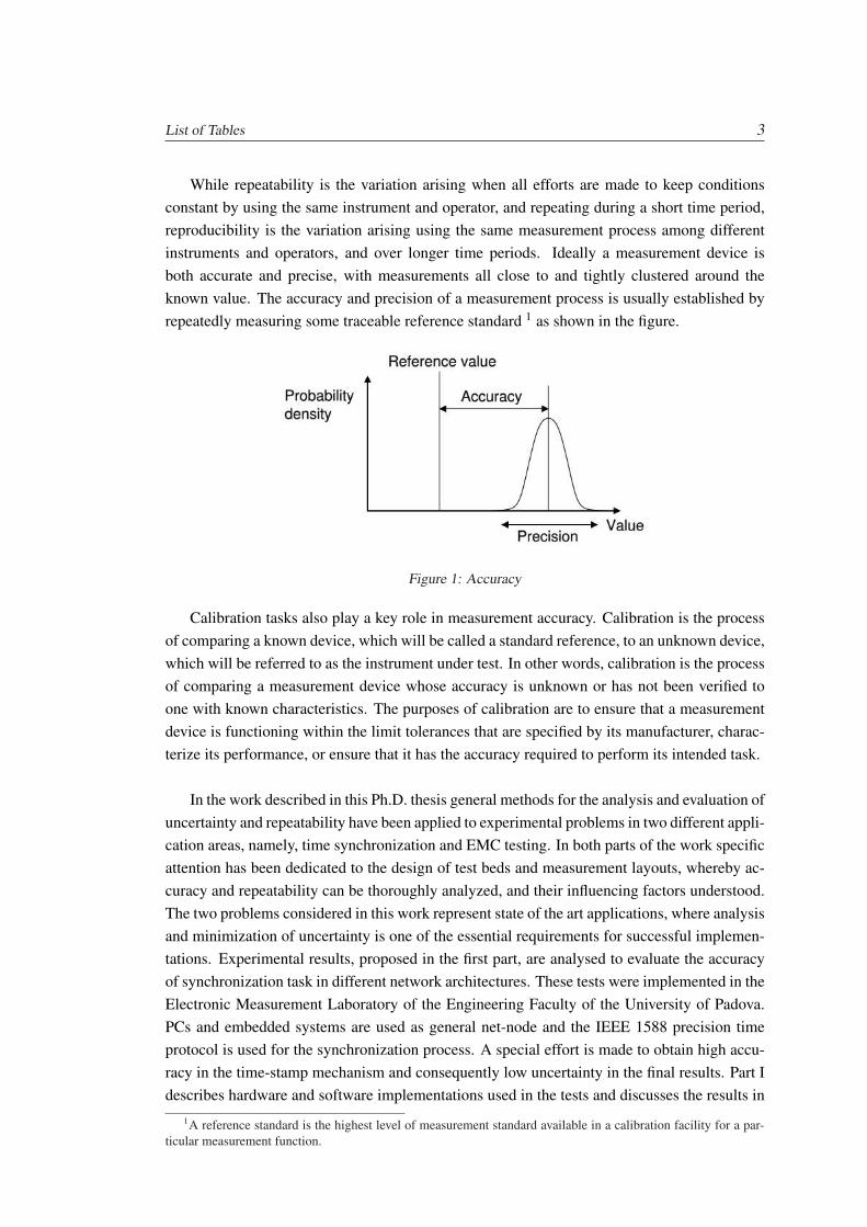
While repeatability is the variation arising when all efforts are made to keep conditionsconstant by using the same instrument and operator, and repeating during a short time period,reproducibility is the variation arising using the same measurement process among differentinstruments and operators, and over longer time periods. Ideally a measurement device isboth accurate and precise, with measurements all close to and tightly clustered around theknown value. The accuracy and precision of a measurement process is usually established byrepeatedly measuring some traceable reference standard 1 as shown in the figure.
Figure 1: Accuracy
Calibration tasks also play a key role in measurement accuracy. Calibration is the processof comparing a known device, which will be called a standard reference, to an unknown device,which will be referred to as the instrument under test. In other words, calibration is the processof comparing a measurement device whose accuracy is unknown or has not been verified toone with known characteristics. The purposes of calibration are to ensure that a measurementdevice is functioning within the limit tolerances that are specified by its manufacturer, charac-terize its performance, or ensure that it has the accuracy required to perform its intended task.
In the work described in this Ph.D. thesis general methods for the analysis and evaluation ofuncertainty and repeatability have been applied to experimental problems in two different appli-cation areas, namely, time synchronization and EMC testing. In both parts of the work specificattention has been dedicated to the design of test beds and measurement layouts, whereby ac-curacy and repeatability can be thoroughly analyzed, and their influencing factors understood.The two problems considered in this work represent state of the art applications, where analysisand minimization of uncertainty is one of the essential requirements for successful implemen-tations. Experimental results, proposed in the first part, are analysed to evaluate the accuracyof synchronization task in different network architectures. These tests were implemented in theElectronic Measurement Laboratory of the Engineering Faculty of the University of Padova.PCs and embedded systems are used as general net-node and the IEEE 1588 precision timeprotocol is used for the synchronization process. A special effort is made to obtain high accu-racy in the time-stamp mechanism and consequently low uncertainty in the final results. Part Idescribes hardware and software implementations used in the tests and discusses the results in
1A reference standard is the highest level of measurement standard available in a calibration facility for a par-ticular measurement function.

4 List of Tables
terms of maximum resolution of synchronization.Electromagnetic compatibility (EMC) tests and calibrations are instead investigated in the sec-ond part. Special devices like an anechoic chamber, open-area test site or climatic chamber arerequired for an accurate analysis, so all these tests were performed in an electronic researchcenter in Padova. Significant results presented in the chapters of Part II regard: (i) some issuesconcerning the measurement accuracy of radiated emission for products in the electromagneticcompatibility test stage, (ii) the accurate calibration of LISN (Line Impedance StabilizationNetwork) focusing on the effects of parasitic parameters, (iii) the analysis of uncertainty con-tributions and repeatability in electrostatic discharge tests.Finally, in chapter 6, experimental results of a research project regarding measurement of in-duced current for TASER application are reported. This project was carried out during a periodat the University of Houston, Department of Electrical and Computer Engineering.
Part I
Analysis of Accuracy in TimeSynchronization

Introduction - Part I
The first part of this thesis introduces the main concepts in time synchronization andpresents some test beds designed to evaluate synchronization performances and accuracy fora generic network environment in a variety of different conditions. The distribution of a timereference has long been a significant research topic in measurement. Over the years, tradi-tional methods based on radio broadcasting have been complemented by satellite-based ref-erence systems (namely, the Global Positioning System, GPS) and, lately, supplemented bynetwork-based time distribution. In fact, local area network (LAN) technology is increasingits importance in the field of instrumentation and measurement, following the adoption of LXI(LAN eXtensions for Instrumentation) as the main support for communication and data ex-change within a measuring system. LANs are also widely used for distributed measurementand control in industrial environments, where restrictive time-constraints must be considered.Analysis on synchronization when no dedicated hardware is present in a node, effects of net-work traffic, as well as the study of timestamping inaccuracies are presented. Tests show thecapabilities and limitations of different network synchronization approaches when a generic,heterogeneous network environment is considered.
Measurement and control systems are widely used in test and measurement, industrial au-tomation, communication systems, electrical power systems and many other areas of moderntechnology. The timing requirements placed on measurement and control systems are becom-ing increasingly stringent. Traditionally these systems have been implemented in a dedicatedarchitecture in which timing constraints are met by careful attention to programming combinedwith communication technologies with deterministic latency. In recent years an increasingnumber of such systems increasingly utilize a distributed architecture and networking tech-nologies. We here intend distributed topology like a system in which hardware componentsare located in geographically diverse areas, consequently networked nodes communicate andcoordinate their actions only by passing messages. When the instrument is part of a distributedmeasurement system, the localization, instrument calibration and time synchronization becomeneeded for accurate measure.Localization is a geographical problem that becomes complex when devices frequently changelocation. Instrument calibration is a more classical topic, some examples are proposed in thenext section of this thesis (Part II). Finally, timing requirements are investigated here, speciallyin term of synchronization among nodes. In systems where devices are located very near toeach other, typically a few meters, sharing a common timing signal is generally the easiest andmost accurate method of synchronization. Instead, sharing a common timing signal becomes

8
unfeasible when the distance between devices increase. Even at moderate distances, e.g. 50meters, a common timing signal may require significant costs for cabling and configuration.This has led to alternate means for enforcing the timing requirements in such systems. Onesuch technique is the use of wired Ethernet communications which are becoming more com-mon in measurement and control applications. In a general network environment the mostwidely used technique for synchronizing the clocks is the Network Time Protocol, NTP, or therelated SNTP.Measurement and control systems have a number of specific requirements that must be met bya clock synchronization technology. In particular:
• Timing accuracies are often in the sub-microsecond range,
• These technologies must be available on a range of networking technologies includingEthernet but also other technologies found in industrial automation and similar indus-tries,
• A minimum of administration is highly desirable,
• The technology must be capable of implementation on low cost and low-end devices,
• The required network and computing resources should be minimal.
The level of precision achievable depends heavily on time jitter (the variation in latency) inthe network also due to the topology. Point-to-point connections provide the highest precision.Hubs impose relatively little network jitter. Under very low or no network load, switches have avery low processing time, typically 2 to 10 µs plus packet reception time, and have low latencyjitter of about 0.4 µs. But with network switches, a single queued maximum length packet im-poses a delay for the following packet of about 122 µs, and under high load conditions, morethan one packet can be in the queue. Variable switch latency means that raw data sent fromtwo different data acquisition nodes to the same receiving node may be delayed differently.Prioritization of packets, eg: IEEE 802.1p, does not fully solve the problem, as at least onelong packet can be in front of a synchronization packet and so will impose up to 122 µs to thejitter of transmission.An effective way to reduce the effect of jitter in Ethernet networks is the use of dedicated sys-tem components that contain real-time clocks or transparent switches. However this solutionpresents some practical problems specially for the high costs. The commonly used switchedEthernet is a preferred solution for many applications due to the price decrease, high band-width, priority features (e.g. VoIP) and the ready availability of Ethernet switches and Ethernetenabled products fulfilling industrial environment requirements. In this case switch latency willvary depending on the switch load. This implies time jitter in synchronization mechanism thatcan be solved if the raw data are time stamped 2. The receiving node can resend the incomingraw data based on the time stamps, and raw data from several acquisitions can be correctlycompared. So, devices periodically exchange information and adjust their local timing sourcesto match each other.
2Time Stamp: is the operation for denoting the date and/or time at which a certain event occurred.
9
IEEE 1588
The timing accuracy that can be achieved in a LAN based on switched Ethernet, where timesynchronization data is distributed via general infrastructure, depends on two factors:
1. Time stamping of incoming and outgoing time packets. Time stamping shall preferablybe performed at the lowest possible level in the OSI protocol stack in order to avoid thevariable latency through the protocol stack.
2. Variable network latency. The switch latency depends on the network load, drop linkspeed, packet sizes and the switch architecture.
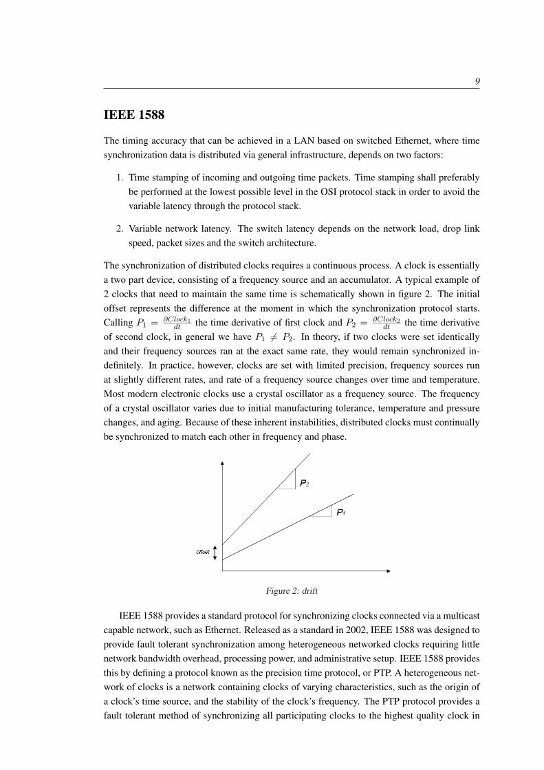
The synchronization of distributed clocks requires a continuous process. A clock is essentiallya two part device, consisting of a frequency source and an accumulator. A typical example of2 clocks that need to maintain the same time is schematically shown in figure 2. The initialoffset represents the difference at the moment in which the synchronization protocol starts.Calling P1 = ∂Clock1
dt the time derivative of first clock and P2 = ∂Clock2dt the time derivative
of second clock, in general we have P1 6= P2. In theory, if two clocks were set identicallyand their frequency sources ran at the exact same rate, they would remain synchronized in-definitely. In practice, however, clocks are set with limited precision, frequency sources runat slightly different rates, and rate of a frequency source changes over time and temperature.Most modern electronic clocks use a crystal oscillator as a frequency source. The frequencyof a crystal oscillator varies due to initial manufacturing tolerance, temperature and pressurechanges, and aging. Because of these inherent instabilities, distributed clocks must continuallybe synchronized to match each other in frequency and phase.
Figure 2: drift
IEEE 1588 provides a standard protocol for synchronizing clocks connected via a multicastcapable network, such as Ethernet. Released as a standard in 2002, IEEE 1588 was designed toprovide fault tolerant synchronization among heterogeneous networked clocks requiring littlenetwork bandwidth overhead, processing power, and administrative setup. IEEE 1588 providesthis by defining a protocol known as the precision time protocol, or PTP. A heterogeneous net-work of clocks is a network containing clocks of varying characteristics, such as the origin ofa clock’s time source, and the stability of the clock’s frequency. The PTP protocol provides afault tolerant method of synchronizing all participating clocks to the highest quality clock in
10
Sync
t1
t2
dm2s=t1-t2
Follow_Up
Delay_Req
t3
t4
ds2m=t3-t4
offset-from-master
Delay_Resp
one-way delay
SlaveMaster
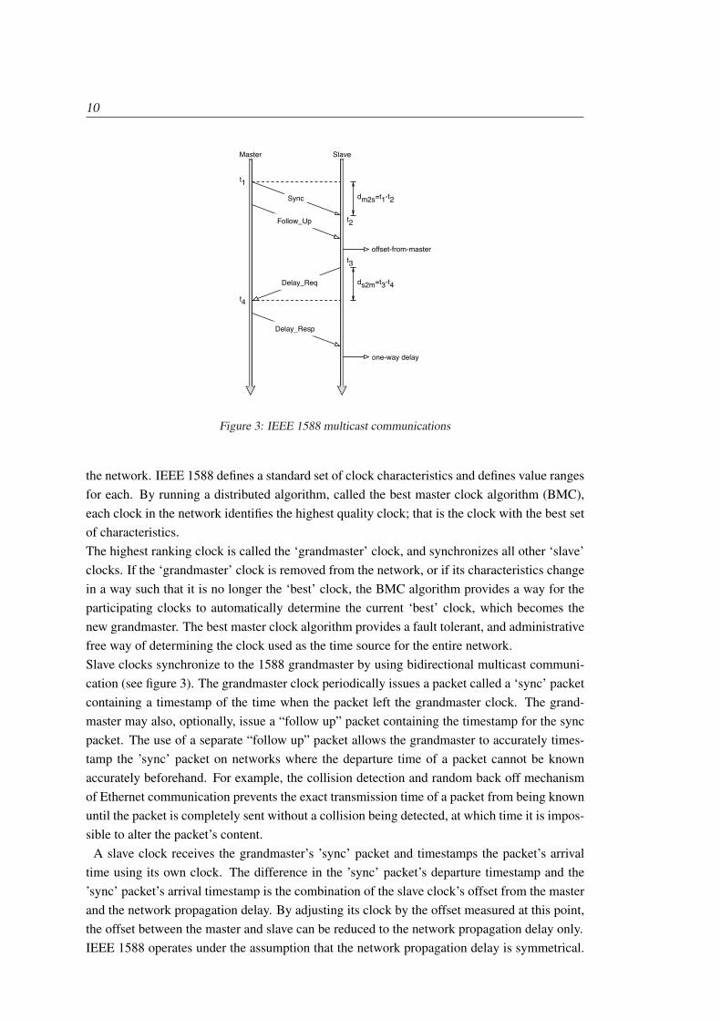
Figure 3: IEEE 1588 multicast communications
the network. IEEE 1588 defines a standard set of clock characteristics and defines value rangesfor each. By running a distributed algorithm, called the best master clock algorithm (BMC),each clock in the network identifies the highest quality clock; that is the clock with the best setof characteristics.The highest ranking clock is called the ‘grandmaster’ clock, and synchronizes all other ‘slave’clocks. If the ‘grandmaster’ clock is removed from the network, or if its characteristics changein a way such that it is no longer the ‘best’ clock, the BMC algorithm provides a way for theparticipating clocks to automatically determine the current ‘best’ clock, which becomes thenew grandmaster. The best master clock algorithm provides a fault tolerant, and administrativefree way of determining the clock used as the time source for the entire network.Slave clocks synchronize to the 1588 grandmaster by using bidirectional multicast communi-cation (see figure 3). The grandmaster clock periodically issues a packet called a ‘sync’ packetcontaining a timestamp of the time when the packet left the grandmaster clock. The grand-master may also, optionally, issue a “follow up” packet containing the timestamp for the syncpacket. The use of a separate “follow up” packet allows the grandmaster to accurately times-tamp the ’sync’ packet on networks where the departure time of a packet cannot be knownaccurately beforehand. For example, the collision detection and random back off mechanismof Ethernet communication prevents the exact transmission time of a packet from being knownuntil the packet is completely sent without a collision being detected, at which time it is impos-sible to alter the packet’s content.
A slave clock receives the grandmaster’s ’sync’ packet and timestamps the packet’s arrivaltime using its own clock. The difference in the ’sync’ packet’s departure timestamp and the’sync’ packet’s arrival timestamp is the combination of the slave clock’s offset from the masterand the network propagation delay. By adjusting its clock by the offset measured at this point,the offset between the master and slave can be reduced to the network propagation delay only.IEEE 1588 operates under the assumption that the network propagation delay is symmetrical.
11
That is, the delay of a packet sent from the master to the slave is the same as the delay of apacket sent from the slave to the master. By making this assumption, the slave can discover,and compensate for the propagation delay. It accomplishes this by issuing a ’delay request’packet which is time stamped on departure from the slave. The ’delay request’ message isreceived and time stamped by the master clock, and the arrival timestamp is sent back to theslave clock in a ’delay response’ packet. The difference in these two timestamps is the networkpropagation delay.By sending and receiving these synchronization packets, the slave clocks can accurately mea-sure the offset between their local clock and the master’s clock. The slaves can then adjusttheir clocks by this offset to match the time of the master. The IEEE 1588 specification doesnot include any standard implementation for adjusting a clock; it merely provides a standardprotocol for exchanging these messages, allowing devices from different manufacturers, andwith different implementations to interoperate.One of the most common implementation is PTPd (daemon) described in [13]. PTPd is a com-plete implementation of the IEEE 1588 specification and the source code is freely availableunder a BSD-style license.

Chapter 1
Test Bed description
In this chapter two different test beds for synchronization analysis are proposed. As recalled inthe introduction, PTP synchronization relies on the exchange of data packets containing times-tamps. In the net, timestamps are generated both by the node acting as time reference and bythe node which requires synchronization. The end result depends on two main factors: times-tamping accuracy and symmetry of packet propagation delays.The aim of the investigation is to understand how accurate a software implementation of PTPcan be. As noted before, dedicated hardware can be effective, but expensive solutions. Sincesoftware-only implementations of the PTP protocol have been proposed on the literature, it isinteresting to understand their potential as well as their limitations, in view of their much morelimited cost.Software timestamping is affected by many concurrent activities in a computer system, likekernel tasks, intensive disk IO or other traffic in the network interface. It is well known that,to achieve high accuracy, timestamping should be performed at the Media Access Control(MAC) level within the network interface card. If software-only implementations are consid-ered, packet time-stamping needs to be implemented as a real-time activity within the operatingsystem kernel and enjoy high priority. To this aim special solutions are used in the proposedtests: in the first case using a real-time operating system, in the second one using embeddedsystems.The PTP implementation employed for these works is the PTP daemon (PTPd) discussed inthe introduction.
1.1 Timing accuracy of scheduled software tasks
An operating system (commonly abbreviated OS) is the software component of a computersystem that is responsible for the management and coordination of activities and the sharingof computer resources. The operating system acts as a host for applications that are run on themachine. As a host, one of the purposes of an operating system is to handle the details of theoperation of the hardware. This relieves application programs from having to manage thesedetails and makes it easier to write applications. Almost all computers, including handheldcomputers, desktop computers, supercomputers, and even video game consoles, use an operat-

14 Chapter 1. Test Bed description
ing system of some type. Some of the oldest models may however use an embedded operatingsystem, that may be contained on a compact disk or other data storage device.Operating systems offer a number of services to application programs and users. Applicationsaccess these services through application programming interfaces (APIs) or system calls. Byinvoking these interfaces, the application can request a service from the operating system, passparameters, and receive the results of the operation (figure 1.1). Executing a program involves
Figure 1.1: A layer structure showing where Operating System is located on generally usedsoftware systems on desktops
the creation of a process by the operating system. The kernel creates a process by setting asideor allocating some memory, loading program code from a disk or another part of memory intothe newly allocated space, and starting it running.Interrupts are central to operating systems as they allow the operating system to deal with theunexpected activities of running programs and the world outside the computer. Interrupt-basedprogramming is one of the most basic forms of time-sharing, being directly supported by mostCPUs. Interrupts provide a computer with a way of automatically running specific code inresponse to events. Even very basic computers support hardware interrupts, and allow the pro-grammer to specify code which may be run when that event takes place.When an interrupt is received, the computer’s hardware automatically suspends whatever pro-gram is currently running by pushing the current state on a stack, and its registers and programcounter are also saved. This is analogous to placing a bookmark in a book when someone isinterrupted by a phone call. This task requires no operating system as such, but only that theinterrupt be configured at an earlier time.In modern operating systems, interrupts are handled by the operating system’s kernel. Inter-rupts may come from either the computer’s hardware, or from the running program. When ahardware device triggers an interrupt, the operating system’s kernel decides how to deal withthis event, generally by running some processing code, or ignoring it. The processing of hard-ware interrupts is a task that is usually delegated to software called device drivers, which maybe either part of the operating system’s kernel, part of another program, or both. Device driversmay then relay information to a running program by various means.A program may also trigger an interrupt to the operating system, which are very similar infunction. If a program wishes to access hardware for example, it may interrupt the operatingsystem’s kernel, which causes control to be passed back to the kernel. The kernel may thenprocess the request which may contain instructions to be passed onto hardware, or to a device
1.1. Timing accuracy of scheduled software tasks 15
driver. When a program wishes to allocate more memory, launch or communicate with anotherprogram, or signal that it no longer needs the CPU, it does so through interrupts.
Common contemporary operating systems include Microsoft Windows, Mac OS, Linuxand Solaris. Microsoft Windows has a significant majority of market share in the desktop andnotebook computer markets, however for applications where a hard layer access is requiredLinux systems represent the best solutions. Linux is a standard time-sharing operating systemwhich provides good average performance and highly sophisticated services. Linux suffersfrom a lack of real time support. To obtain a timing correctness behavior, it is necessary tomake some changes in the kernel sources, i.e. in the interrupt handling and scheduling poli-cies. In this way, you can have a real time platform, with low latency and high predictabilityrequirements, within full non real time Linux environment (access to TCP/IP, graphical displayand windowing systems, file and data base systems, etc.).
1.1.1 RTAI Extension
Accuracy in recording the interrupt time is essential. The operation should be implementedby a specific real-time software task within the operating system kernel; for this reason a real-time operating system (RTOS) is required, so that a deterministic time from event to systemresponse is ensured []. A real time system can be defined as a “system capable of guaranteeingtiming requirements of the processes under its control”. In fact, an RTOS does not necessarilyhave high throughput; rather, an RTOS provides facilities which, if used properly, guaranteedeadlines can be met generally (soft real-time) or deterministically (hard real-time). An RTOSwill typically use specialized scheduling algorithms in order to provide the real-time developerwith the tools necessary to produce deterministic behavior in the final system. An RTOS isvalued more for how quickly and/or predictably it can respond to a particular event than forthe given amount of work it can perform over time. Key factors in an RTOS are therefore aminimal interrupt latency and a minimal thread switching latency.Since an interrupt handler blocks the highest priority task from running, and since real timeoperating systems are designed to keep thread latency to a minimum, interrupt handlers are typ-ically kept as short as possible. The interrupt handler defers all interaction with the hardwareas long as possible; typically all that is necessary is to acknowledge or disable the interrupt (sothat it won’t occur again when the interrupt handler returns). The interrupt handler then queueswork to be done at a lower priority level, often by unblocking a driver task (through releasinga semaphore or sending a message). The scheduler often provides the ability to unblock a taskfrom interrupt handler context.
The choice for the RTOS used in the tests fell on RTAI (Real Time Application Interface[]). It is a real-time extension for the Linux kernel - which allows the implementation ofapplications with strict timing constraints. RTAI is a patch to the standard Linux kernel and alibrary which has a hardware abstraction layer, a real-time scheduler and real-time interprocesscommunication (IPC) services. RTAI offers the same services of the Linux kernel core, addingthe features of an industrial real time operating system. It consists basically of an interrupt
16 Chapter 1. Test Bed description
dispatcher: RTAI mainly traps the peripherals interrupts and if necessary re-routes them toLinux. It is not an intrusive modification of the kernel; it uses the concept of HAL (hardwareabstraction layer) to get information from Linux and to trap some fundamental functions. ThisHAL provides few dependencies to Linux Kernel. RTAI considers Linux as a backgroundtask running when no real time activity occurs. Since the documentations describe simpleand easy the adaptation in the Linux kernel, our experience in the RTAI installation was verycomplicated. In fact it requires a good knowledge in Linux systems and kernel configurations.
1.1.2 Time response performance
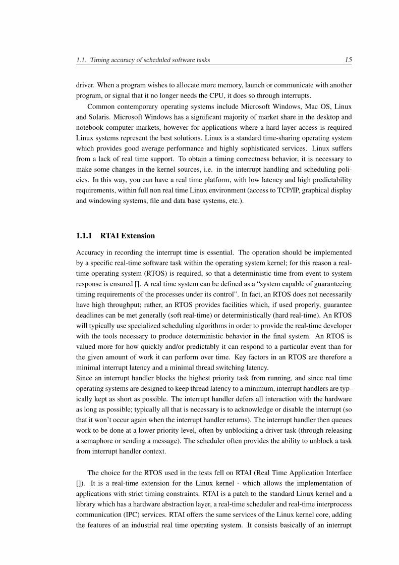
This paragraph shows the results obtained when measuring real-time behaviour of a RTAI-Linux operating system running on standard PC platforms. During this study, we’ve focusedon a comparison of the time response in the RTAI system with respect to a non real time system.In particular, we have measured the time elapsed between the interrupt signal activation andthe start of the interrupt routine, via counter values stored in a digital oscilloscope.The schematic representation of test bed is reported in figure 1.2. The signal generated by
Figure 1.2: Parallel-test
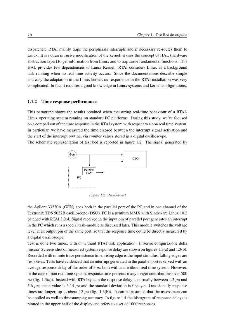
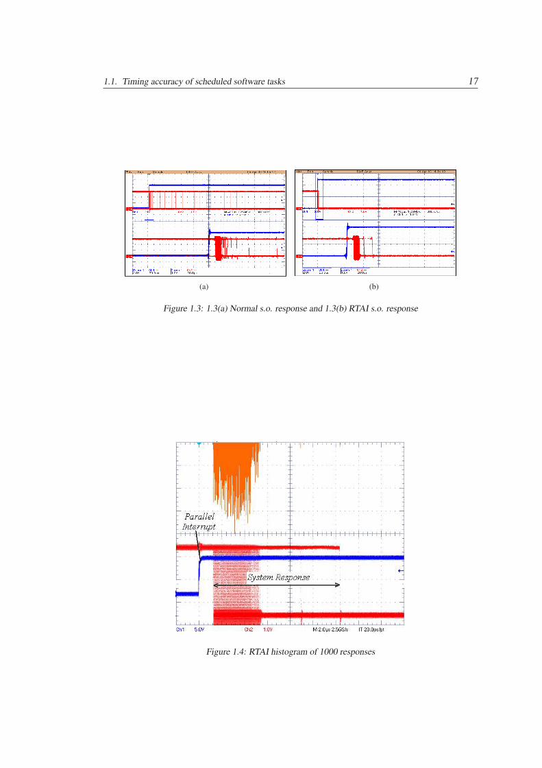
the Agilent 33220A (GEN) goes both in the parallel port of the PC and in one channel of theTektronix TDS 5032B oscilloscope (DSO). PC is a pentium MMX with Slackware Linux 10.2patched with RTAI 3.0r4. Signal received in the input pin of parallel port generates an interruptin the PC which runs a special task-module as discussed later. This module switches the voltagelevel at an output pin of the same port, so that the response time could be directly measured bya digital oscilloscope.Test is done two times, with or without RTAI task application. (inserire cofigurazione dellamisura) Screens shot of measured system response delay are shown on figures 1.3(a) and 1.3(b).Recorded with infinite trace persistence time, rising edge is the input stimulus, falling edges areresponses. Tests have evidenced that an interrupt generated in the parallel port is served with anaverage response delay of the order of 3 µs both with and without real time system. However,in the case of non real time system, response time presents many longer contributions over 500µs (fig. 1.3(a)). Instead with RTAI system the response delay is normally between 1.2 µs and5.6 µs; mean value is 3.14 µs and the standard deviation is 0.94 µs. Occasionally responsetimes are longer, up to about 12 µs (fig. 1.3(b)). It can be assumed that the assessment canbe applied as well to timestamping accuracy. In figure 1.4 the histogram of response delays isplotted in the upper half of the display and refers to a set of 1000 responses.
1.1. Timing accuracy of scheduled software tasks 17
(a) (b)
Figure 1.3: 1.3(a) Normal s.o. response and 1.3(b) RTAI s.o. response
Figure 1.4: RTAI histogram of 1000 responses
18 Chapter 1. Test Bed description
1.2 First Test Bed Implementation - PC nodes with backgroundtraffic
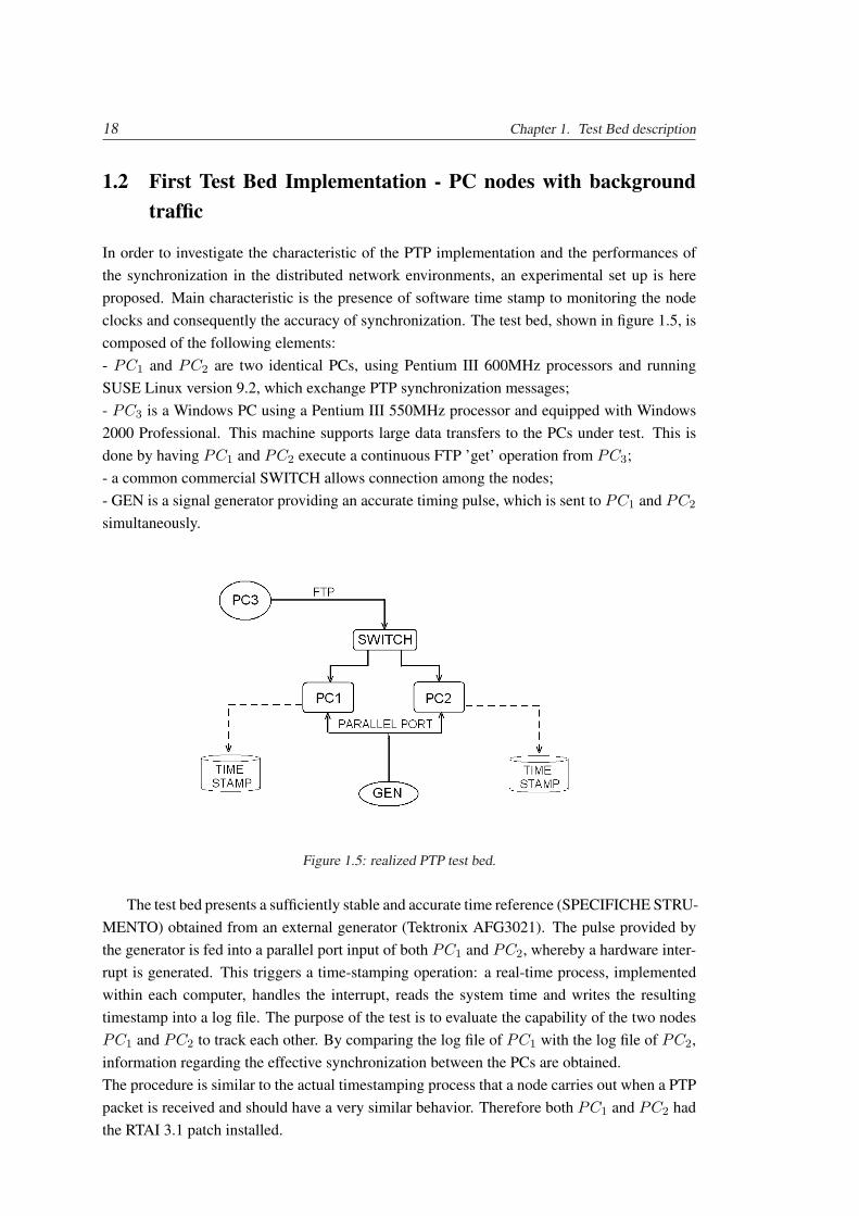
In order to investigate the characteristic of the PTP implementation and the performances ofthe synchronization in the distributed network environments, an experimental set up is hereproposed. Main characteristic is the presence of software time stamp to monitoring the nodeclocks and consequently the accuracy of synchronization. The test bed, shown in figure 1.5, iscomposed of the following elements:- PC1 and PC2 are two identical PCs, using Pentium III 600MHz processors and runningSUSE Linux version 9.2, which exchange PTP synchronization messages;- PC3 is a Windows PC using a Pentium III 550MHz processor and equipped with Windows2000 Professional. This machine supports large data transfers to the PCs under test. This isdone by having PC1 and PC2 execute a continuous FTP ’get’ operation from PC3;- a common commercial SWITCH allows connection among the nodes;- GEN is a signal generator providing an accurate timing pulse, which is sent to PC1 and PC2
simultaneously.
Figure 1.5: realized PTP test bed.
The test bed presents a sufficiently stable and accurate time reference (SPECIFICHE STRU-MENTO) obtained from an external generator (Tektronix AFG3021). The pulse provided bythe generator is fed into a parallel port input of both PC1 and PC2, whereby a hardware inter-rupt is generated. This triggers a time-stamping operation: a real-time process, implementedwithin each computer, handles the interrupt, reads the system time and writes the resultingtimestamp into a log file. The purpose of the test is to evaluate the capability of the two nodesPC1 and PC2 to track each other. By comparing the log file of PC1 with the log file of PC2,information regarding the effective synchronization between the PCs are obtained.The procedure is similar to the actual timestamping process that a node carries out when a PTPpacket is received and should have a very similar behavior. Therefore both PC1 and PC2 hadthe RTAI 3.1 patch installed.
1.2. First Test Bed Implementation - PC nodes with background traffic 19
The code used for software time stamp is reported below:
# i n c l u d e < l i n u x / module . h># i n c l u d e < r t a i . h># i n c l u d e < r t a i _ s c h e d . h>
# d e f i n e BASEPORT 0 x378
i n t c o u n t =0;s t r u c t t i m e v a l t v a l ;
s t a t i c vo id h a n d l e r ( void )
c o u n t ++;d o _ g e t t i m e o f d a y (& t v a l ) ;ou tb_p ( count , BASEPORT ) ;r t _ p r i n t k ( " >>> t imes t amp = %d \ t ; %d \ n " , t v a l . t v _ s e c , t v a l . t v _ u s e c ) ;r t _ a c k _ i r q ( 7 ) ;
i n t x i n i t _ m o d u l e ( void )
i n t r e t ;r e t = r t _ r e q u e s t _ g l o b a l _ i r q ( 7 , ( void ∗ ) h a n d l e r ) ;r t _ e n a b l e _ i r q ( 7 ) ;ou tb_p (0 x10 , BASEPORT + 2 ) ; / / s e t p o r t t o i n t e r r u p t mode ; p i n s are o u t p u td o _ g e t t i m e o f d a y (& t v a l ) ;r t _ p r i n t k ( " >>> i n i z i o = %d \ t ; %d \ n " , t v a l . t v _ s e c , t v a l . t v _ u s e c ) ;r t _ s e t _ o n e s h o t _ m o d e ( ) ;re turn 0 ;
void xc leanup_module ( void )
r t _ p r i n t k ( " Unload ing p a r a l l e l p o r t l a t e n c y t e s t \ n " ) ;r t _ d i s a b l e _ i r q ( 7 ) ;r t _ f r e e _ g l o b a l _ i r q ( 7 ) ;
m o d u l e _ i n i t ( x i n i t _ m o d u l e ) ;m o d u l e _ e x i t ( xc leanup_module ) ;MODULE_LICENSE( "GPL" ) ;
To simulate traffic into the LAN, another program can be run in the PCs under test, whichperforms continuous downloads from the FTP server with a speed of about 32 Mbps over FastEthernet for each PC (total: 64 Mbps). Inclusion of the FTP server PC3 in the architectureallows the assessment of PTP performances in a network carrying a significant and unbalancedtraffic load. It is also important to assess the effects of different degrees of activity in thenodes. To simulate computer activities in a controlled way, two programs were written; one(CPU-jam) keeps the CPU busy and another (disk-jam) forces the PC to continuously write dataon its hard disk. For most tests we used a normal 100Mb Ethernet switch without boundary
20 Chapter 1. Test Bed description
clock, while a 10Mb Ethernet switch was used to simulate a network bottleneck.
1.3 Second Solution - Synchronization with emulated cross-traffic
We now shall take a more general view of the synchronization problem and consider genericnetwork environments where distributed measurement may coexist with other network appli-cations. An example is provided by a system where instruments or sensor nodes exchange datawhile sharing the same network infrastructure with applications such as network printers, IPtelephony and so on. It should be remembered that timing protocols are only one facet of thesynchronization problem. In fact, the protocol has the task of assuring that accurate timinginformation are propagated to all nodes within a synchronization domain. The next step is theimplementation of a suitable procedure for regulating the local clock, ensuring that it tracks thereference to within desired bounds (this is sometimes called a clock servo). In generic networkenvironments it is also necessary to account for at least two other factors: one is the presenceof traffic, which causes the packets carrying timing information to suffer from variability inpropagation time; the other is the degree of accuracy with which time is recorded, by packettimestamping, at different nodes.In the next tests the network nodes are two embedded systems Linux based.
1.3.1 Embedded Systems
An embedded system is a special-purpose computer system designed to perform one or a fewdedicated functions,[!!] often with real-time computing constraints. It is usually embeddedas part of a complete device including hardware and mechanical parts. In contrast, a general-purpose computer, such as a personal computer, can do many different tasks depending onprogramming. Embedded systems control many of the common devices in use today.
Since the embedded system is dedicated to specific tasks, design engineers can optimize it,reducing the size and cost of the product, or increasing the reliability and performance. Someembedded systems are mass-produced, benefiting from economies of scale.
Physically, embedded systems range from portable devices such as digital watches andMP3 players, to large stationary installations like traffic lights, factory controllers, or the sys-tems controlling nuclear power plants. Complexity varies from low, with a single microcon-troller chip, to very high with multiple units, peripherals and networks mounted inside a largechassis or enclosure.
In general, ‘embedded system’ is not an exactly defined term, as many systems have someelement of programmability. For example, Handheld computers share some elements with em-bedded systems - such as the operating systems and microprocessors which power them - butare not truly embedded systems, because they allow different applications to be loaded andperipherals to be connected.
Embedded systems are interesting for this work because they typically allow lower levelaccess to system resources. It can be assumed that the system clock is among the accessible

1.3. Second Solution - Synchronization with emulated cross-traffic 21
resources which that modifications are faster and less affected by jitter.
The system chosen for the tests is the FOX Board [3]. The FOX Board is an EmbeddedLinux Core Engine with reduced size and low power requirements. This system has an ETRAX100LX microprocessor, a 100MIPS RISC CPU made by Axis Communications and 16MB ofRAM. Presents some interfaces like Ethernet 10/100Mb port, 2 USB host 1.1, slots for two20x2 pin strip step with 48 I/O lines, I2C bus, SPI, serial and parallel ports. Through the eth-ernet interface it is possible to have access to the internal Web server, FTP server, SSH, Telnetand the complete TCP/IP stack. Moreover, a free and Open Source Software Development Kitare available which enables a strong customization of Linux Kernel.
1.3.2 Test Bed
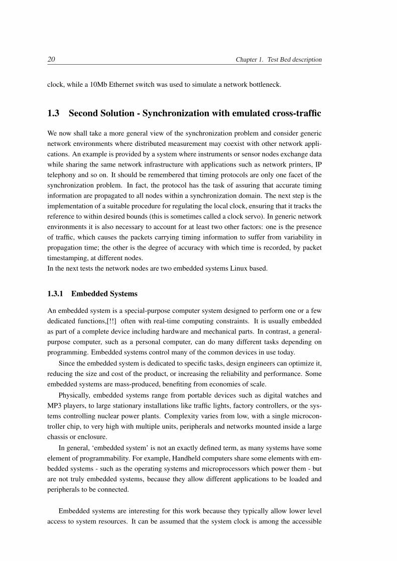
A schematic representation of the test bed is illustrated in figure 1.6. Node 1 and Node 2represent the systems that need to execute simultaneous operations at a given time. For thispurpose they must first be synchronized by a suitable protocol. The Source node generatescross-traffic with a given profile towards the Sink node, the latter simply destroying the receivedpackets. The Hub is used to allow communication among the nodes which, in real life, mightbe separated by a whole network. In a more complex test environment, its place could be takenby a network emulator (such as, for instance, NIST Net); however, for the aims of this worka hub is enough, since it fulfills the basic purpose of mixing the timing packets exchangedbetween the two nodes with an external packet flow designed to reproduce the desired trafficprofile. To monitoring the traffic, there is one measure point. It consist on one PC with DAGcard 1 which allows to capture all packets into the net.
Figure 1.6: Test environment.
The test bed configuration differs from the previously one, where a Source node interactswith either Node 1 or Node 2, causing it to carry out data transfers. The latter is representativeof the case when a remote measuring instrument needs to send significant amounts of data overthe network. This set up considers instead the more common case where accurate time refer-
1DAG network monitoring interface cards provide 100% packet or cell capture, regardless of interface type,packet size, or network loading.
22 Chapter 1. Test Bed description
encing is an important issue, but measuring nodes generate and exchange limited amounts ofdata. Cross-traffic then assumes a great importance when the performance of synchronizationprotocols must be evaluated in networks characterized by the convergence of different appli-cations. In this context it plays an important role and needs to be accurately modeled. Theemphasis of the tests is on the effects of cross-traffic on the one-way delay of packets contain-ing timing information.
1.3.3 Cross traffic generation
Different strategies can be adopted to emulate cross-traffic, however some constraints must betaken into account. First of all traffic models must reproduce real traffic properties, which arewell described in the literature [6], in a general way not limited to some specific situation. Thisis a very important feature since there is a rapid evolution in network applications and in theirbehavior, so the attention must not be focused on a particular scenario.
It is also desirable to handle models whose parameters have a physical meaning and thatcan be strictly controlled to evaluate synchronization issues under well defined test conditions.
We chose to model packet traffic using ON/OFF sources that can be modeled with chaoticmaps. This analytical model is able to accurately and concisely represent network traffic, inparticular its strong correlation at all the time scales of engineering interest. This property,usually known as long range dependence (LRD), leads to a self-similar model of traffic. TheHurst parameter H [6] provides a measure of traffic correlation degree and needs to be takeninto account since it strongly affects delays in network buffers.
Chaotic maps, proposed as traffic model in [7], are low dimensional nonlinear systemswhose time evolution is described by the knowledge of an initial state and a set of dynamicallaws. The traffic generator is an ON/OFF source that sends one packet when the source is inthe ON state, while no packets are transmitted when the source is in the OFF state. A one-dimensional chaotic map is used to describe state changes. This map has a state variable xnthat evolves over time according to the nonlinear system:
xn+1 = f1(xn), if: 0 < xn ≤ dthat is:yn = 0; (1.1)
xn+1 = f2(xn), if: d < xn < 1that is:yn = 1, (1.2)
where yn is the indicator variable, describing the state of the source during the n-th timeinterval [(n− 1) cotT, n · T ). If the indicator variable is zero the source is OFF, while if yn isequal to 1 the source is ON.
The functions f1(xn) and f2(xn) are respectively given by:
f1(xn) = xn + (1− d)(xn
d
)m1
(1.3)
f2(xn) = xn − d
(1− xn
1− d
)m2
(1.4)
where m1, m2 ∈ (1, 2) and d ∈ (0, 1) are the parameters of the map.
1.3. Second Solution - Synchronization with emulated cross-traffic 23
The average number of packets generated by the map represents the traffic load λ , whichis related to the probability that the source is in the ON region. Analytical approximations forcalculating the traffic load can be found in the literature and are out of the scope of this paper.However it is important to note that this traffic parameter is strongly dependent on the mapparameter d, which specifies the ratio between the ON and OFF region. In particular, the valueof λ is greater for d near to zero, while it becomes smaller as d tends to 1.
1.3.4 Implementation issues
The proposed ON-OFF chaotic traffic source has been implemented by using the client-serverparadigm. In this implementation the server represents the traffic Source of figure 1.6, whilethe client represents the traffic Sink. At the client side, the user sets the source parametersm1, m2, d and T . These parameters are successively sent to the server by using a controlchannel over TCP in order to obtain a reliable communication. After receiving the sourceparameters, the server starts to send UDP packets toward the client as specified by the chaoticmap described in this paragraph. We chose the UDP transport protocol to generate cross-trafficin order to avoid packet retransmissions and in general flow control, that otherwise wouldmodify the statistical traffic model. The control channel is finally used by the client to stoptraffic generation.
Some remarks need to be carefully considered in cross-traffic generation. In fact there isa strict relationship between the time step T of the packet generator at the source and the datarate R of the real system. Let Nb be the byte length of packets generated by the traffic source.This means that a packet takes a time equal to Tp = Nb/R to be transmitted over the wire. Theratio Tp/T provides the percentage of bandwidth occupied by the source.
The need to carry out tests with a realistic bandwidth occupation translates into a designrequirement for the test bed. At present, T is limited to a minimum value of 1 ms by the Javaimplementation. Then, for a 100 Mb/s network, if Nb = 500, the packet time is Tp = 40 µs
and Tp/T = 4%, which is too low for the presence of cross-traffic to have some effect onthe system. Since the actual implementation of traffic source cannot generate packets overshorter intervals, the other solution consists in slowing down the system rate by a time rescalingoperation. Therefore by choosing a 10 Mb/s network, Nb = 500 byte and T = 1 ms weobtain Tp = 400 µs and Tp/T = 40%. Finally, a bandwidth occupation equal to 100% can beobtained if the byte length of the packet is set to Nb = 1, 250 byte.
1.3.5 Validation of the traffic generator
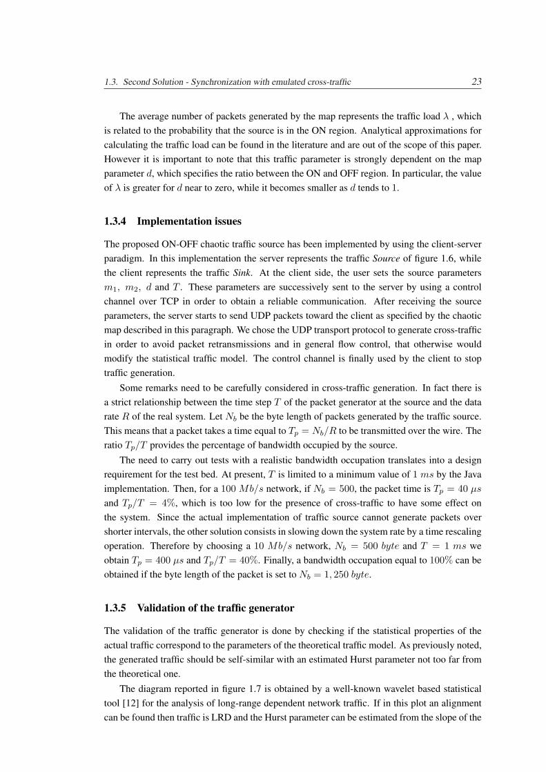
The validation of the traffic generator is done by checking if the statistical properties of theactual traffic correspond to the parameters of the theoretical traffic model. As previously noted,the generated traffic should be self-similar with an estimated Hurst parameter not too far fromthe theoretical one.
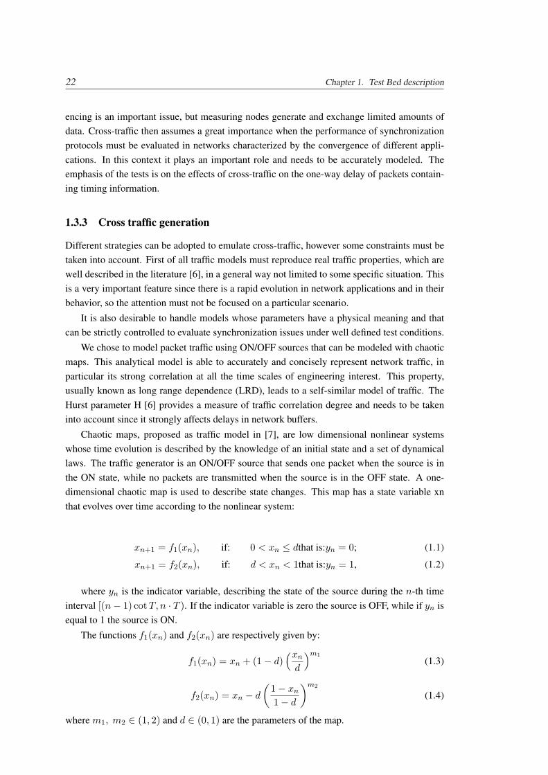
The diagram reported in figure 1.7 is obtained by a well-known wavelet based statisticaltool [12] for the analysis of long-range dependent network traffic. If in this plot an alignmentcan be found then traffic is LRD and the Hurst parameter can be estimated from the slope of the
24 Chapter 1. Test Bed description
2 4 6 8 10 12 14 164
6
8
10
12
14
Scale j
yj
H=0.766
Figure 1.7: Hurst parameter estimation from measured data.
regression line. In this case, that corresponds to traffic used in Sec. VI.B, the estimated Hurstparameter is equal to H = 0.77 that is in good agreement with the theoretical value H = 0.78.

Chapter 2
Synchronization Tests and Analysis
In this chapter tests carried out with different network setups are presented and discusses.Using the first test bed we observed: i) how long PTPd takes to achieve synchronization, towithin a specified tolerance, starting from a given time offset; ii) the effective tracking accuracythat can be reached; iii) possible anomalies and events requiring more detailed analysis; iv)critical conditions that can influence PTP synchronization. The aim of the second test bed is toexplore the capabilities and limitations of different network synchronization approaches whena generic, heterogeneous network environment is considered.
2.1 Preliminary Investigations
Using the first test bed proposed in 1.2 some tests have been conducted.
2.1.1 Single Clock Analysis
The two clocks of PC1 and PC2 were first measured separately. The generator was set toprovide a reference pulse every 30 s (30 PPS) and the two PCs were left running free withoutPTPd. Tests evidence that both clocks are skewed with respect to the reference: PC1 loses onaverage 33.4 µs/sec, while PC2 loses on average 41.1 µs/sec (figure 2.1). Variability is limitedto a range of ±0.12 µs/s; this agrees very well with the timing variability shown in figure1.4. Although the room where tests were carried out has no temperature control, conditionsremained reasonably stable, therefore it can be assumed that the skew between the clocks ofPC1 and PC2 has a constant value of about 7.8 µs/s. The PTP master sends a SYNC messageover the network once every 2 s; in this time interval the estimated offset between PC1 andPC2 in the test bed would be about 15 µs.
2.1.2 Performance limits
In the first test PC1 and PC2 were directly connected via a cross cable. No other activity wasundertaken and the link was free from other network traffic, allowing to assess the upper limitof synchronization performances. A reference timing pulse was generated every 30 s also inthis case.
26 Chapter 2. Synchronization Tests and Analysis
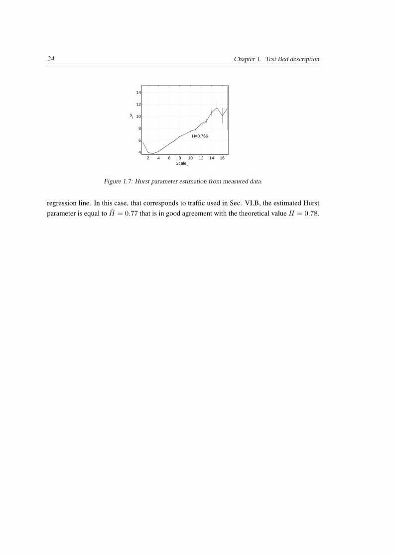
Figure 2.1: single clock of PC1 and PC2
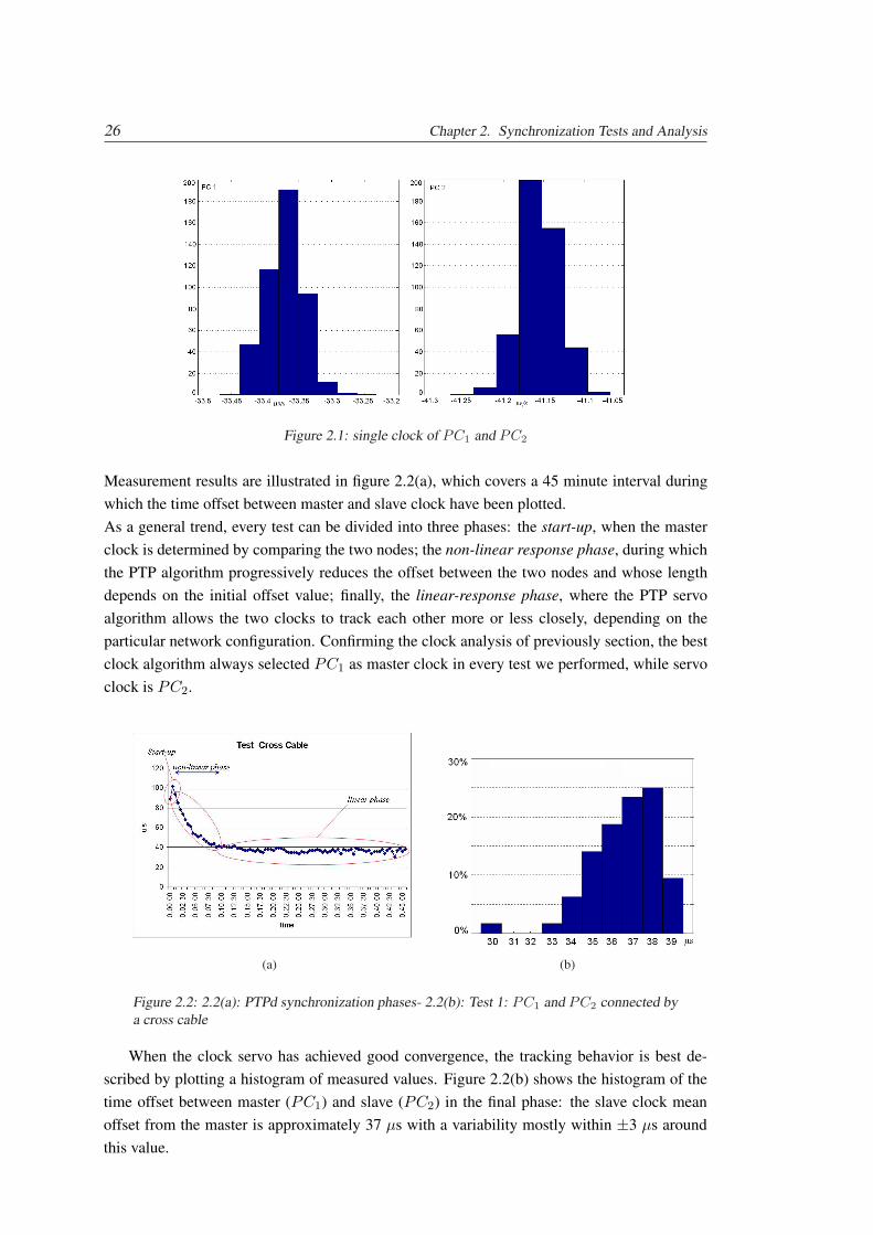
Measurement results are illustrated in figure 2.2(a), which covers a 45 minute interval duringwhich the time offset between master and slave clock have been plotted.As a general trend, every test can be divided into three phases: the start-up, when the masterclock is determined by comparing the two nodes; the non-linear response phase, during whichthe PTP algorithm progressively reduces the offset between the two nodes and whose lengthdepends on the initial offset value; finally, the linear-response phase, where the PTP servoalgorithm allows the two clocks to track each other more or less closely, depending on theparticular network configuration. Confirming the clock analysis of previously section, the bestclock algorithm always selected PC1 as master clock in every test we performed, while servoclock is PC2.
(a) (b)
Figure 2.2: 2.2(a): PTPd synchronization phases- 2.2(b): Test 1: PC1 and PC2 connected bya cross cable
When the clock servo has achieved good convergence, the tracking behavior is best de-scribed by plotting a histogram of measured values. Figure 2.2(b) shows the histogram of thetime offset between master (PC1) and slave (PC2) in the final phase: the slave clock meanoffset from the master is approximately 37 µs with a variability mostly within ±3 µs aroundthis value.
2.1. Preliminary Investigations 27
We did not analyze in detail the causes of the delay but, given the nature of the connection, itseems reasonable to assume that any possible path asymmetry would have to be related to thetransmit and receive operations within the nodes. On the other hand, the extent of variability isstill in good agreement with that of timestamping which, in this very simple configuration, isclearly the main factor of timing uncertainty.
2.1.3 Network switch
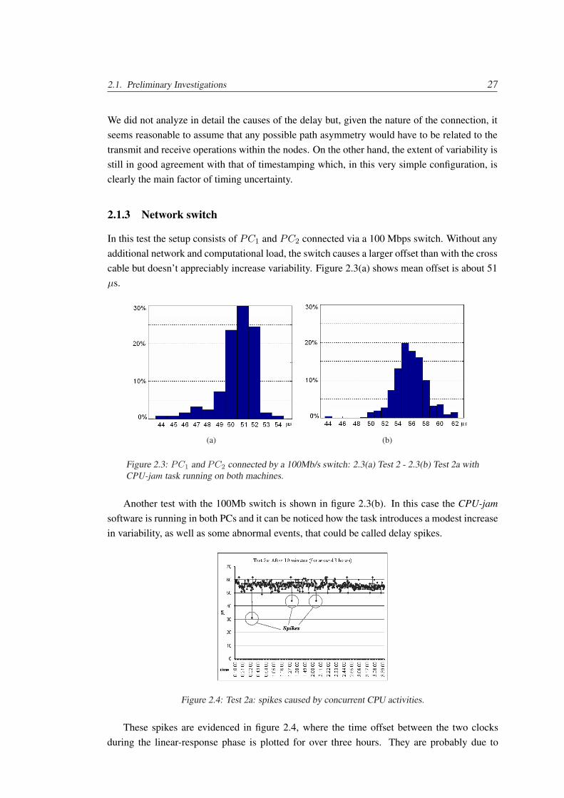
In this test the setup consists of PC1 and PC2 connected via a 100 Mbps switch. Without anyadditional network and computational load, the switch causes a larger offset than with the crosscable but doesn’t appreciably increase variability. Figure 2.3(a) shows mean offset is about 51µs.
(a) (b)
Figure 2.3: PC1 and PC2 connected by a 100Mb/s switch: 2.3(a) Test 2 - 2.3(b) Test 2a withCPU-jam task running on both machines.
Another test with the 100Mb switch is shown in figure 2.3(b). In this case the CPU-jamsoftware is running in both PCs and it can be noticed how the task introduces a modest increasein variability, as well as some abnormal events, that could be called delay spikes.
Figure 2.4: Test 2a: spikes caused by concurrent CPU activities.
These spikes are evidenced in figure 2.4, where the time offset between the two clocksduring the linear-response phase is plotted for over three hours. They are probably due to
28 Chapter 2. Synchronization Tests and Analysis
occasional situations where system resources for the real-time timestamping procedure cannotbe released immediately, resulting in incorrect timestamp values.
2.1.4 Network traffic
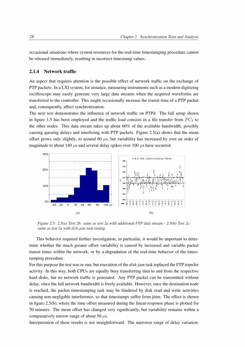
An aspect that requires attention is the possible effect of network traffic on the exchange ofPTP packets. In a LXI system, for instance, measuring instruments such as a modern digitizingoscilloscope may easily generate very large data streams when the acquired waveforms aretransferred to the controller. This might occasionally increase the transit time of a PTP packetand, consequently, affect synchronization.The next test demonstrates the influence of network traffic on PTPd. The full setup shownin figure 1.5 has been employed and the traffic load consists in a file transfer from PC3 tothe other nodes. This data stream takes up about 60% of the available bandwidth, possiblycausing queuing delays and interfering with PTP packets. Figure 2.5(a) shows that the meanoffset grows only slightly, to around 60 µs, but variability has increased by over an order ofmagnitude to about 140 µs and several delay spikes over 100 µs have occurred.
(a) (b)
Figure 2.5: 2.5(a) Test 2b: same as test 2a with additional FTP data stream - 2.5(b) Test 2c:same as test 2a with disk-jam task runing.
This behavior required further investigation; in particular, it would be important to deter-mine whether the much greater offset variability is caused by increased and variable packettransit times within the network, or by a degradation of the real-time behavior of the times-tamping procedure.For this purpose the test was re-run, but execution of the disk-jam task replaced the FTP transferactivity. In this way, both CPUs are equally busy transferring data to and from the respectivehard disks, but no network traffic is generated. Any PTP packet can be transmitted withoutdelay, since the full network bandwidth is freely available. However, once the destination nodeis reached, the packet timestamping task may be hindered by disk read and write activitiescausing non-negligible interference, so that timestamps suffer from jitter. The effect is shownin figure 2.5(b), where the time offset measured during the linear-response phase is plotted for50 minutes. The mean offset has changed very significantly, but variability remains within acomparatively narrow range of about 50 µs.Interpretation of these results is not straightforward. The narrower range of delay variation,
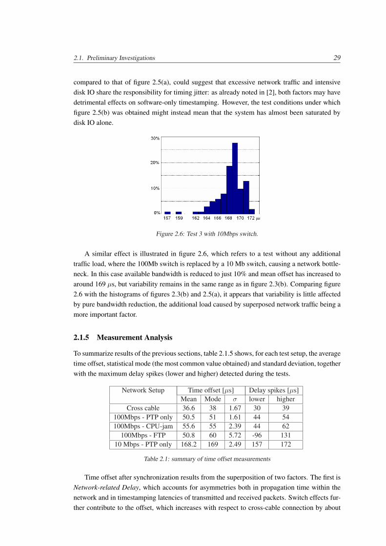
2.1. Preliminary Investigations 29
compared to that of figure 2.5(a), could suggest that excessive network traffic and intensivedisk IO share the responsibility for timing jitter: as already noted in [2], both factors may havedetrimental effects on software-only timestamping. However, the test conditions under whichfigure 2.5(b) was obtained might instead mean that the system has almost been saturated bydisk IO alone.
Figure 2.6: Test 3 with 10Mbps switch.
A similar effect is illustrated in figure 2.6, which refers to a test without any additionaltraffic load, where the 100Mb switch is replaced by a 10 Mb switch, causing a network bottle-neck. In this case available bandwidth is reduced to just 10% and mean offset has increased toaround 169 µs, but variability remains in the same range as in figure 2.3(b). Comparing figure2.6 with the histograms of figures 2.3(b) and 2.5(a), it appears that variability is little affectedby pure bandwidth reduction, the additional load caused by superposed network traffic being amore important factor.
2.1.5 Measurement Analysis
To summarize results of the previous sections, table 2.1.5 shows, for each test setup, the averagetime offset, statistical mode (the most common value obtained) and standard deviation, togetherwith the maximum delay spikes (lower and higher) detected during the tests.
Network Setup Time offset [µs] Delay spikes [µs]Mean Mode σ lower higher
Cross cable 36.6 38 1.67 30 39100Mbps - PTP only 50.5 51 1.61 44 54100Mbps - CPU-jam 55.6 55 2.39 44 62
100Mbps - FTP 50.8 60 5.72 -96 13110 Mbps - PTP only 168.2 169 2.49 157 172
Table 2.1: summary of time offset measurements
Time offset after synchronization results from the superposition of two factors. The first isNetwork-related Delay, which accounts for asymmetries both in propagation time within thenetwork and in timestamping latencies of transmitted and received packets. Switch effects fur-ther contribute to the offset, which increases with respect to cross-cable connection by about
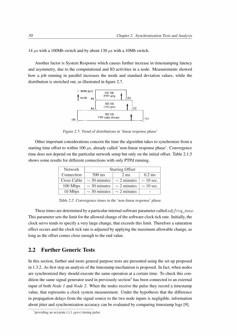
30 Chapter 2. Synchronization Tests and Analysis
14 µs with a 100Mb switch and by about 130 µs with a 10Mb switch.
Another factor is System Response which causes further increase in timestamping latencyand asymmetry, due to the computational and IO activities in a node. Measurements showedhow a job running in parallel increases the mode and standard deviation values, while thedistribution is stretched out, as illustrated in figure 2.7.
Figure 2.7: Trend of distributions in ’linear response phase’
Other important considerations concern the time the algorithm takes to synchronize from astarting time offset to within 100 µs, already called ’non-linear response phase’. Convergencetime does not depend on the particular network setup but only on the initial offset. Table 2.1.5shows some results for different connections with only PTPd running.
Network Starting OffsetConnection 500 ms 2 ms 0.2 msCross Cable ∼ 30 minutes ∼ 2 minutes ∼ 10 sec.100 Mbps ∼ 30 minutes ∼ 2 minutes ∼ 10 sec.10 Mbps ∼ 30 minutes ∼ 2 minutes -
Table 2.2: Convergence times in the ’non-linear response’ phase.
These times are determined by a particular internal software parameter called adjfreq_max.This parameter sets the limit for the allowed change of the software clock tick rate. Initially, theclock servo tends to specify a very large change, that exceeds this limit. Therefore a saturationeffect occurs and the clock tick rate is adjusted by applying the maximum allowable change, aslong as the offset comes close enough to the end value.
2.2 Further Generic Tests
In this section, further and more general purpose tests are presented using the set up proposedin 1.3.2. As first step an analysis of the timestamp mechanism is proposed. In fact, when nodesare synchronized they should execute the same operation at a certain time. To check this con-dition the same signal generator used in previously section1 has been connected to an externalinput of both Node 1 and Node 2. When the nodes receive the pulse they record a timestampvalue, that represents a clock system measurement. Under the hypothesis that the differencein propagation delays from the signal source to the two node inputs is negligible, informationabout jitter and synchronization accuracy can be evaluated by comparing timestamp logs [9].
1providing an accurate (±1 ppm) timing pulse
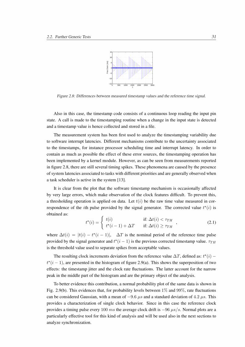
2.2. Further Generic Tests 31
0 500 1000 1500 2000 2500 3000−15
−10
−5
0
5
10
15
s
Fre
e C
lock
[m
s]
Figure 2.8: Differences between measured timestamp values and the reference time signal.
Also in this case, the timestamp code consists of a continuous loop reading the input pinstate. A call is made to the timestamping routine when a change in the input state is detectedand a timestamp value is hence collected and stored in a file.
The measurement system has been first used to analyze the timestamping variability dueto software interrupt latencies. Different mechanisms contribute to the uncertainty associatedto the timestamps, for instance processor scheduling time and interrupt latency. In order tocontain as much as possible the effect of these error sources, the timestamping operation hasbeen implemented by a kernel module. However, as can be seen from measurements reportedin figure 2.8, there are still several timing spikes. These phenomena are caused by the presenceof system latencies associated to tasks with different priorities and are generally observed whena task scheduler is active in the system [13].
It is clear from the plot that the software timestamp mechanism is occasionally affectedby very large errors, which make observation of the clock features difficult. To prevent this,a thresholding operation is applied on data. Let t(i) be the raw time value measured in cor-respondence of the ith pulse provided by the signal generator. The corrected value t?(i) isobtained as:
t?(i) =
t(i) if: ∆t(i) < τTH
t?(i− 1) + ∆T if: ∆t(i) ≥ τTH, (2.1)
where ∆t(i) = |t(i) − t?(i − 1)|, ∆T is the nominal period of the reference time pulseprovided by the signal generator and t?(i− 1) is the previous corrected timestamp value. τTH
is the threshold value used to separate spikes from acceptable values.
The resulting clock increments deviation from the reference value ∆T , defined as: t?(i)−t?(i− 1), are presented in the histogram of figure 2.9(a). This shows the superposition of twoeffects: the timestamp jitter and the clock rate fluctuations. The latter account for the narrowpeak in the middle part of the histogram and are the primary object of the analysis.
To better evidence this contribution, a normal probability plot of the same data is shown inFig. 2.9(b). This evidences that, for probability levels between 1% and 99%, rate fluctuationscan be considered Gaussian, with a mean of −9.6 µs and a standard deviation of 4.2 µs. Thisprovides a characterization of single clock behavior. Since in this case the reference clockprovides a timing pulse every 100 ms the average clock drift is −96 µs/s. Normal plots are aparticularly effective tool for this kind of analysis and will be used also in the next sections toanalyze synchronization.
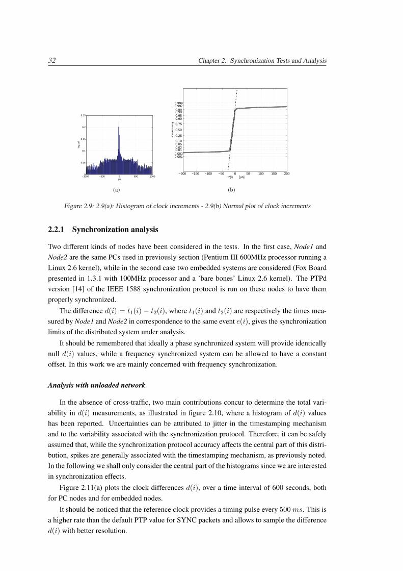
32 Chapter 2. Synchronization Tests and Analysis
−1000 −500 0 500 10000
0.05
0.1
0.15
0.2
0.25
µs
log
(a)
−200 −150 −100 −50 0 50 100 150 200
0.0010.0030.01 0.02 0.05 0.10
0.25
0.50
0.75
0.90 0.95 0.98 0.99 0.9970.999
t*(i) [µs]
Pro
babi
lity
(b)
Figure 2.9: 2.9(a): Histogram of clock increments - 2.9(b) Normal plot of clock increments
2.2.1 Synchronization analysis
Two different kinds of nodes have been considered in the tests. In the first case, Node1 andNode2 are the same PCs used in previously section (Pentium III 600MHz processor running aLinux 2.6 kernel), while in the second case two embedded systems are considered (Fox Boardpresented in 1.3.1 with 100MHz processor and a ’bare bones’ Linux 2.6 kernel). The PTPdversion [14] of the IEEE 1588 synchronization protocol is run on these nodes to have themproperly synchronized.
The difference d(i) = t1(i) − t2(i), where t1(i) and t2(i) are respectively the times mea-sured by Node1 and Node2 in correspondence to the same event e(i), gives the synchronizationlimits of the distributed system under analysis.
It should be remembered that ideally a phase synchronized system will provide identicallynull d(i) values, while a frequency synchronized system can be allowed to have a constantoffset. In this work we are mainly concerned with frequency synchronization.
Analysis with unloaded network
In the absence of cross-traffic, two main contributions concur to determine the total vari-ability in d(i) measurements, as illustrated in figure 2.10, where a histogram of d(i) valueshas been reported. Uncertainties can be attributed to jitter in the timestamping mechanismand to the variability associated with the synchronization protocol. Therefore, it can be safelyassumed that, while the synchronization protocol accuracy affects the central part of this distri-bution, spikes are generally associated with the timestamping mechanism, as previously noted.In the following we shall only consider the central part of the histograms since we are interestedin synchronization effects.
Figure 2.11(a) plots the clock differences d(i), over a time interval of 600 seconds, bothfor PC nodes and for embedded nodes.
It should be noticed that the reference clock provides a timing pulse every 500 ms. This isa higher rate than the default PTP value for SYNC packets and allows to sample the differenced(i) with better resolution.
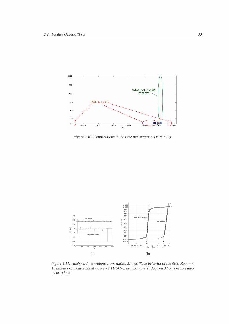
2.2. Further Generic Tests 33
Figure 2.10: Contributions to the time measurements variability.
0 100 200 300 400 500 600−400
−300
−200
−100
0
100
200
300
d(i)
[µs
]
s
PC nodes
Embedded nodes
(a)
−150 −100 −50 0 50 100 150 200
0.0010.0030.01 0.02 0.05 0.10
0.25
0.50
0.75
0.90 0.95 0.98 0.99 0.9970.999
t*(i) [µs]
Pro
babi
lity
Embedded nodes
PC nodes
(b)
Figure 2.11: Analysis done without cross-traffic. 2.11(a) Time behavior of the d(i). Zoom on10 minutes of measurement values - 2.11(b) Normal plot of d(i) done on 3 hours of measure-ment values
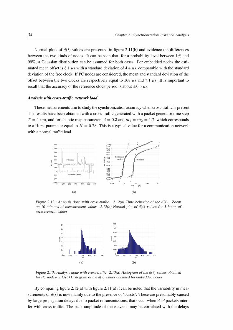
34 Chapter 2. Synchronization Tests and Analysis
Normal plots of d(i) values are presented in figure 2.11(b) and evidence the differencesbetween the two kinds of nodes. It can be seen that, for a probability level between 1% and99%, a Gaussian distribution can be assumed for both cases. For embedded nodes the esti-mated mean offset is 3.1 µs with a standard deviation of 4.4 µs, comparable with the standarddeviation of the free clock. If PC nodes are considered, the mean and standard deviation of theoffset between the two clocks are respectively equal to 168 µs and 7.1 µs. It is important torecall that the accuracy of the reference clock period is about ±0.5 µs.
Analysis with cross-traffic network load
These measurements aim to study the synchronization accuracy when cross-traffic is present.The results have been obtained with a cross-traffic generated with a packet generator time stepT = 1 ms, and for chaotic map parameters d = 0.3 and m1 = m2 = 1.7, which correspondsto a Hurst parameter equal to H = 0.78. This is a typical value for a communication networkwith a normal traffic load.
0 100 200 300 400 500 600−300
−200
−100
0
100
200
300
400
500
600
700
d(i)
[µs
]
s
PC nodes
Embedded nodes
(a)
−200 0 200 400 600
0.0010.0030.01 0.02 0.05 0.10
0.25
0.50
0.75
0.90 0.95 0.98 0.99 0.9970.999
t*(i) [µs]
Pro
babi
lity Embedded
nodes PC nodes
(b)
Figure 2.12: Analysis done with cross-traffic. 2.12(a) Time behavior of the d(i). Zoomon 10 minutes of measurement values- 2.12(b) Normal plot of d(i) values for 3 hours ofmeasurement values
−400 −200 0 200 400 600 8000
0.1
0.2
0.3
0.4
0.5
0.6
0.7
µs
log
(a)
−400 −200 0 200 400 600 8000
0.05
0.1
0.15
0.2
0.25
0.3
0.35
µs
log
(b)
Figure 2.13: Analysis done with cross-traffic. 2.13(a) Histogram of the d(i) values obtainedfor PC nodes- 2.13(b) Histogram of the d(i) values obtained for embedded nodes
By comparing figure 2.12(a) with figure 2.11(a) it can be noted that the variability in mea-surements of d(i) is now mainly due to the presence of ‘bursts’. These are presumably causedby large propagation delays due to packet retransmissions, that occur when PTP packets inter-fer with cross-traffic. The peak amplitude of these events may be correlated with the delays

2.2. Further Generic Tests 35
introduced by the medium-access control policy implemented by the physical layer. The timeduration instead depends on the impulse response of the PTP clock servo and on the clock driftcorrection mechanism. The latter effect can be noted by comparing the bursts obtained withthe two different kinds of nodes: the shape is the same for a given system set-up, independentlyfrom the amplitude, while it changes if another system is taken into account.
In figure 2.12(b) the normal probability plots of d(i) values have been reported. It canbe noted that the two distributions are quite similar, as can be seen also in the histograms offigures 2.13(a) and 2.13(b). Both largely differ from a Gaussian model, this makes no sense toestimate the mean and standard deviation from the normal probability plot.


Part II
Calibration and Repeatability in EMCTests


Introduction - Part II
Part II of the thesis, dealing with some specific problems related to uncertainty and re-peatability in Electromagnetic Compatibility (EMC) Tests, is organized as follows. In Chap-ter 3, some considerations about magnetic field propagation within an anechoic chamber arereported. Simulation analysis and experiments have been performed for magnetic radiatingcircuits (magnetic loop). In Chapter 4 an accurate calibration of Line Impedance StabilizationNetworks (LISN) is presented, focusing on the effects of parasitic parameters at the EquipmentUnder Test (EUT) port. Finally, in Chapter 5 the uncertainty contributions associated to themeasurement for air electrostatic discharge (ESD) immunity tests are analyzed. The effects ofdifferent type A uncertainty contributions are compared and the ESD repeatability is assessed.
Electromagnetic compatibility (EMC) is the branch of electrical sciences which studies theunintentional generation, propagation and reception of electromagnetic energy with referenceto the unwanted effects (Electromagnetic Interference, or EMI) that such energy may induce.
The effects of EMI are extremely variable in character and magnitude, ranging from simpleannoyance to catastrophe. Some examples of the potential effects of EMI are:
• interference to television and radio reception,
• loss of data in digital systems or in transmission of data,
• delay in production of equipment exhibiting intra-unit, subsystem, or system-level EMI,
• malfunction of medical electronic equipment, automotive control, navigation equipment.
The goal of EMC is the correct operation, in the same electromagnetic environment, of dif-ferent equipment which use electromagnetic phenomena, and the avoidance of any interferenceeffects.
In order to achieve this, EMC pursues two different kinds of issues. Emission issues are re-lated to the unwanted generation of electromagnetic energy, and to the countermeasures whichshould be taken in order to reduce such generation and to avoid the escape of any remainingenergy into the external environment. Susceptibility or immunity issues, in contrast, refer to thecorrect operation of electrical equipment in the presence of unplanned electromagnetic distur-bances.
Interference, or noise, mitigation and hence electromagnetic compatibility is achieved byaddressing both emission and susceptibility issues, i.e., attenuating the sources of interference,
40
making the coupling path between source and victim less efficient, and making the potentialvictim systems less vulnerable.In electromagnetic compatibility contexts measurement uncertainty estimation is a critical fac-tor, since it plays an essential role in the decision on the conformity/nonconformity of a productto applicable standards. Furthermore, the subject of measurement uncertainty in EMC test isvery complex because the equipment that is being tested was not designed specifically for thetest (i.e. there is no ’EMC’ connection port), the test method usually includes set-up factorsthat affect the measurement, the test equipment is often itself complex and includes severalseparated but interconnected components, and finally the variations between different test sitesmight compromise measurement reproducibility.
EMI/EMC Test Lab
EMI/EMC Laboratories test equipment can be configured to perform specific tests to investi-gate the limits of compliance in terms of electromagnetic interference and ensure that all thedesigned circuits meet the basic EMI standards in terms of electromagnetic emission and im-munity. The generic standards [15] [16] list a series of phenomena which should be tested, likeconducted and radiated emissions or ESD transient and surge immunity. Most product stan-dards cover the same phenomena, although there may be exceptions and additions, so often itis not necessary for all of the phenomena to be tested at all stages.EMC tests mainly concern two different specific types of tests: for pre-compliance or fullcompliance.
Pre-compliance. While a product is in development, the EMC effects of alternative designdecisions and of remedial measures will need to be checked. Different layouts, different filtersand different screening regimes need to be compared and this should be done as developmentprogresses rather than at its conclusion, as otherwise a design which is ineffective in EMCterms may have excessive development resources spent on it. Therefore there is a need for adiagnostic test facility - which needs not be truly equivalent to the compliance test set-up - tobe available throughout the development phase. Once a prototype is ready, this represents themodel which will be subject to full compliance testing and it is advisable to carry out somepreliminary tests to the same standards. This has several purposes:- to avoid unpleasant surprises. If a product is clearly well outside the required limits, it ispointless submitting it to the compliance test before remedial work has brought it to a point atwhich there is a reasonable chance of success;- to define the worst-case configuration and operating mode. For a complex product with manyoptions, modes and configurations, the worst case to submit for full compliance may not beimmediately obvious and finding it may take much longer than the test itself;- to define the criteria for immunity test failure. It may not be clear until this point exactly whathappens to the product when it is subjected to incoming transient or RF interference. It is themanufacturer’s responsibility to define what actually constitutes a test failure in the immunitycontext.
Full compliance. A full compliance test set-up must be capable of carrying out all those

41
tests that the manufacturer intends to do in-house, to the required standard setup. The choiceof which tests to do in-house and which at an external test house is affected by several factors,the most prominent being:- the available budget, skills and resources- the nature of the EUT(s)- the requirements of the applicable standards
Set-up for EMC tests are reported in the product standards with many technical details. How-ever, EMI measurements may significantly affect the parameter measured, resulting in error.For instance, the location of antennas may affect the calibration curve error also around 30dB in undamped shielded-room measurements of radiated emissions. A measurement with anoscilloscope may corrupt the measured signal as a result of either the additional ground connec-tion or by radiated pick up on the oscilloscope test leads. Moreover ground loop connections,cable route, attenuator mismatch, external environment conditions are some possible causes ofinaccurate measure. The next chapters describe some of these critical measurement conditions.
EMC measurements could be influenced by different setup conditions such as table posi-tioning [2] and table material [3], and conducted emissions could be influenced by factors suchas length [4], height, and manner of main cable meandering [5] as well as positioning of theequipment under test [6].
Standards
The level of immunity into equipment depends on how critical the correct functioning of theequipment is and on the electromagnetic environment in which it is designed to operate. ManyEMI requirements take the criticality and environment into account by classifying equipmentand by imposing different susceptibility test levels in the different classes.EMI can be considered a form of environmental pollution: in order to reduce the impact ofthis pollution, some control on the environmental level of conducted and radiated emissions ofnoise is necessary.Many countries impose commercial regulations on the emission from data-processing equip-ment; industrial, scientific, and medical (ISM) equipment; vehicles; appliances; etc. The ma-jority of military regulations and standards, and some commercial specifications, also requirethat equipment be demonstrated immune to susceptibility test levels.Commercial requirements are typically confined to limits on conducted and radiated emis-sions. However, with the advent of European Union (EU) EMC Directive, mandatory androutine immunity (susceptibility) test requirements were imposed for the first time on commer-cial equipment. The EMC requirements encompass equipment from RF ac welders to electricdrills, household equipment, and digital device.

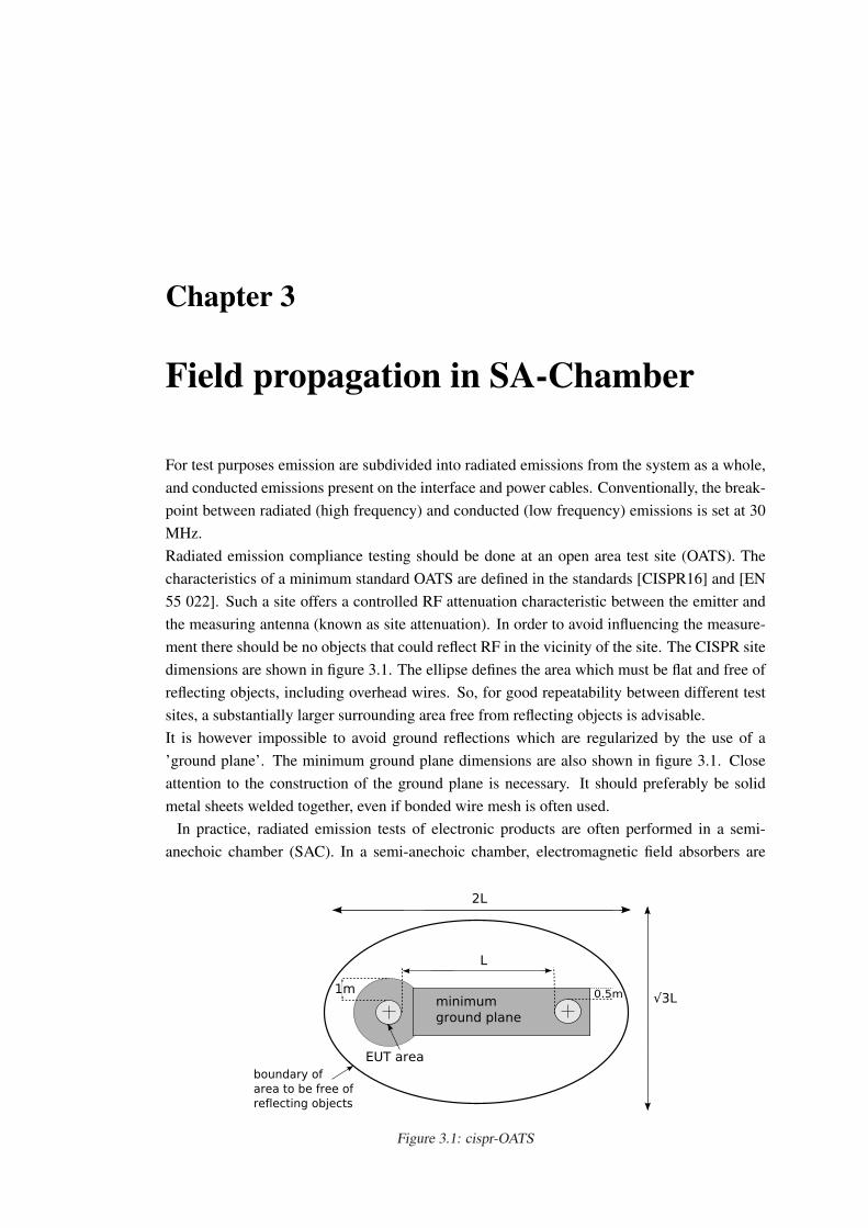
Chapter 3
Field propagation in SA-Chamber
For test purposes emission are subdivided into radiated emissions from the system as a whole,and conducted emissions present on the interface and power cables. Conventionally, the break-point between radiated (high frequency) and conducted (low frequency) emissions is set at 30MHz.Radiated emission compliance testing should be done at an open area test site (OATS). Thecharacteristics of a minimum standard OATS are defined in the standards [CISPR16] and [EN55 022]. Such a site offers a controlled RF attenuation characteristic between the emitter andthe measuring antenna (known as site attenuation). In order to avoid influencing the measure-ment there should be no objects that could reflect RF in the vicinity of the site. The CISPR sitedimensions are shown in figure 3.1. The ellipse defines the area which must be flat and free ofreflecting objects, including overhead wires. So, for good repeatability between different testsites, a substantially larger surrounding area free from reflecting objects is advisable.It is however impossible to avoid ground reflections which are regularized by the use of a’ground plane’. The minimum ground plane dimensions are also shown in figure 3.1. Closeattention to the construction of the ground plane is necessary. It should preferably be solidmetal sheets welded together, even if bonded wire mesh is often used.
In practice, radiated emission tests of electronic products are often performed in a semi-anechoic chamber (SAC). In a semi-anechoic chamber, electromagnetic field absorbers are
Figure 3.1: cispr-OATS
44 Chapter 3. Field propagation in SA-Chamber
placed at the chamber walls and ceiling to avoid reflections of the radiated waves and echoes atthe receiver input of the measurement apparatus. The only exception is for the ground plane,which must be a conducting metal plane, without absorbers.In order to reduce the costs due to the expensive absorbing materials and the large dimensionsof the chamber required by the standard, pre-compliance test sites are often realized and fre-quently used. In fact, the distance between EUT and receiving antenna determines the overalldimensions of the site and hence its cost. Three commonly specified distances are 3 m, 10 mand 30 m. Confidence checks can be carried out on a 3m range, on the assumption that levelsmeasured at 10 m will be 10 dB lower (field strength should be proportional to 1/d). This as-sumption is not entirely valid at the lower end of the frequency range where 3m separation isapproaching the near field.Standards define the requirements for screened anechoic enclosures for emission measurement[17]. The major requirement is to establish that the site attenuation is not significantly affectedby wall reflections. To this aim the concept of normalized site attenuation (NSA) is used toestimate the SAC response. NSA is defined in [ANSI C63.4] as the site attenuation divided bythe antenna factors (AFs) of the radiating and receiving antennas (all in linear units). The stan-dard requires NSA values within±4 dB from the theoretical NSA, and over the whole radiatedemission frequency range 30 MHz to 1 GHz. Due to the fact that semi anechoic chambers usu-ally do not satisfy the above recalled criteria in terms of NSA (especially in the lowest rangeof frequency), it is important to investigate the accuracy obtained from the measurements.In the past, several scientific researches have studied the correlation between measurementsperformed in an ideal test site and measurements carried out in some non-compliant sites. In[19], Garn introduced the concept of ’chamber factors’, through which the E field estimatesobtained in a non-compliant site can be corrected in order to achieve values that can be used todirectly verify the compliance of the product to the emission limits. The chamber factor wasalso introduced in [20] along with the concept of ’grey factor’. Despite its effectiveness, the useof correction factors has non-negligible practical drawbacks: it requires a complex handling ofthe general measurement results and, moreover, a number of preliminary reference measure-ments performed in an open area test site (OATS) are always needed.In this chapter a number of simulation analysis and experiments are reported to evaluate thelimits of radiated emission tests when performed within chambers that do not fulfil the NSArequirements. In fact, the repeatability of radiated emission tests and their uncertainty is di-rectly related to the radiating circuits present inside the EUT and even to the external coveragetype and dimensions.
3.1 Chamber Factors
The characterization of a test enclosure in terms of chamber factors requires several measure-ments at different test configurations, i.e. for different transmit antennae (dipole or loop),antenna positions and polarizations. For each configuration, the correction factor can be deter-mined as follows:
3.2. Characterization of the Investigated Test Site 45
CF [dB] = EREF [dBµV/m]−EENC [dBµV/m] (3.1)
where CF is the correction factor, EREF is the field strength measured at the reference site,and EENC is the field strength measured in the enclosure, i.e. the semi-anechoic chamber. Thereference site is a good OATS, i.e. having only very small deviations from the ideal values ofNSA. A dipole and a loop antenna are used as transmit antennae to provide fields with differentwave impedance. A biconical antenna is used as a receive antenna. When plotted in a graph,the values of CF typically appear with a superimposed spread. The upper envelope curve ob-tained is the worst-case chamber factor, while the mean between the upper and lower curve isthe mean chamber factor. The spread of the correction factors is the grey factor.Determined chamber factors can be used to adjust the field strength estimates obtained in ra-diated emission tests of the EUT. In particular, the chamber factors (in dB) are to be added tothe field strength estimates (in dBµV/m) measured in the semi-anechoic chamber in order toobtain the open-site equivalent values (in dBµV/m).Chamber factors are functions of frequency and polarization, and depend on EUT physical fea-tures, such as dimensions and radiating circuit type (loop or dipole-like). Indeed, the absorbersused in the chamber have properties that depend on the wave impedance, which is constantin the far field region, and may vary considerably in the near field one. On the other hand,the extension of near and far field regions is strongly related to the wave frequency and EUTdimensions. Approximately, the near field region includes the points whose distance fromthe EUT is lower than λ, while the far field region includes the points located far away fromthe EUT, by more than 2D2/λ , D being the largest dimension of the EUT. Therefore, uponvarying the frequency and D, the properties of the absorbers may considerably change, and,consequently, the chamber response too.In a pre-compliance analysis of radiated emissions, measurement of the chamber response as afunction of the frequency and EUT dimensions is very essential. To this aim, [18] requires theapplication of the so-called ’volume method’, which consists of measurements to be performedwith the transmit antenna placed at different locations within the volume that a EUT may oc-cupy. A limit of this method is that it does not consider the real effects of the EUT emissions,hence the effects of its possibly large dimensions, i.e. the parameter D. This fact could evenlead to relevant inaccuracy in the estimate of radiated emissions.
3.2 Characterization of the Investigated Test Site
A first set of preliminary experiments has been performed with the aim of characterizing asemi-anechoic chamber of size 7.94 m (L) x 3.74 m (W) x 3.34 m (H). For a good character-ization of this site, three specific investigations have been conducted. The first step consistsof computing the difference of site attenuation with respect to the theoretical reference (NSA).The second one is related to obtaining the chamber factors as described in the previous section.Finally a comparison between the SAC and a self made OATS is presented.
46 Chapter 3. Field propagation in SA-Chamber
3.2.1 NSA Characterization
NSA has been measured according to the approach defined in [18], in the frequency range 30MHz to 1 GHz and with variable step size (1 MHz for 30-100 MHz, 5 MHz for 100-500 MHz,and 10 MHz for 500-1000 MHz). In particular, a couple of biconical and log periodic antennas,one transmit and another receive, have been used in the range 30 - 200 MHz and 200 - 1000MHz, respectively. The antennas have been positioned in the chamber according to the volumemethod and with the transmit antenna located within a cylindrical test volume of 2 m diameter.For each considered frequency and transmit antenna position, a number of measurements havebeen repeated for the two polarizations. The worst-case values obtained are summarized infigure 3.2(a), where the difference (in dB) between the measured and reference NSA is plottedversus frequency. The plot clearly shows that the employed chamber does not satisfy the aboverecalled ±4 dB requirement. In particular, the highest differences are observed in the range 30- 200 MHz.
3.2.2 CF Characterization
Chamber factors have been determined as described in (3.1). In particular, EENC has beenassessed in the semi-anechoic chamber under test, while EREF has been evaluated in the openfield site of Seibersdorf at the Austrian Research Centre. A calibrated reference radiator (Re-fRad 1) has been used to generate the signal. Three antennas have been then connected: adipole of 65 cm length and a square loop of 30 cm side length, in the range 30 - 200 MHz,and a dipole of 20 cm length, in the range 200 - 1000 MHz. The measurement of field strengthhas been carried out by using a biconical antenna in the range 30 - 200 MHz, and a log peri-odic antenna in the range 200 - 1000 MHz. For measurements in the semi-anechoic chamberthe receive antenna has been moved at a scan range of 1 to 2 m above the floor and with ameasurement distance of 3 m. For each considered frequency, transmit antenna type and posi-tion, a number of measurements have been repeated for the two polarizations. The magnitudeof worst-case values obtained are summarized in figure 3.2(b), where the chamber factors areplotted for both horizontal and vertical polarization. The plot shows once again the limits ofthe chamber response, for which significant correction factors are needed.
3.2.3 OATS Characterization
Further NSA measurements have been conducted in an OATS reference site. The self-madeOATS consisted of a 6 m x 7 m conducting ground plane, positioned over a flat concrete groundplane free of obstacles. A picture of this OATS is shown in figure 3.3(a). The conductingground plane has been realized by using two metallic layers, each consisting of 30 cm widthaluminium2 stripes placed side by side with overlaps of about 3 cm. The stripes have been
1RefRad is a battery operated combo generator for producing a well defined field strength in the frequency rangeof 1 MHz to 1 GHz.
2thin aluminium cooking sheets
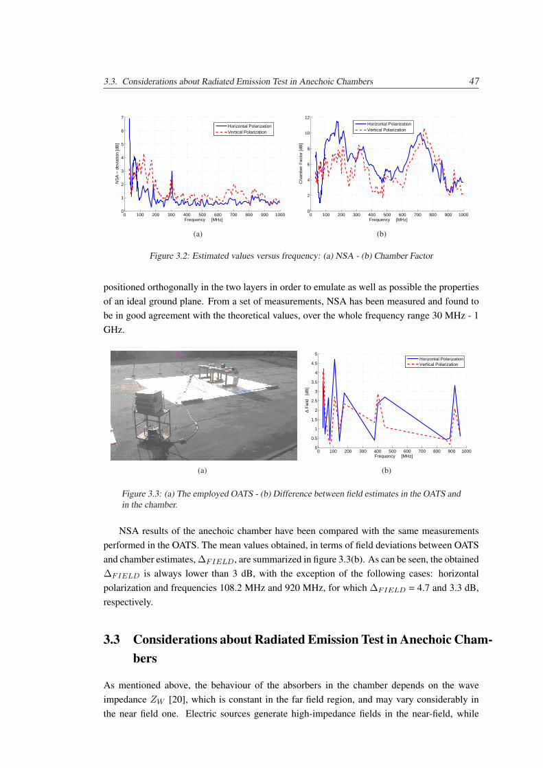
3.3. Considerations about Radiated Emission Test in Anechoic Chambers 47
0 100 200 300 400 500 600 700 800 900 10000
1
2
3
4
5
6
7
Frequency [MHz]
NS
A −
dev
iatio
n [d
B]
Horizontal PolarizationVertical Polarization
(a)
0 100 200 300 400 500 600 700 800 900 10000
2
4
6
8
10
12
Frequency [MHz]
Cha
mbe
r F
acto
r [d
B]
Horizontal PolarizationVertical Polarization
(b)
Figure 3.2: Estimated values versus frequency: (a) NSA - (b) Chamber Factor
positioned orthogonally in the two layers in order to emulate as well as possible the propertiesof an ideal ground plane. From a set of measurements, NSA has been measured and found tobe in good agreement with the theoretical values, over the whole frequency range 30 MHz - 1GHz.
(a)
0 100 200 300 400 500 600 700 800 900 10000
0.5
1
1.5
2
2.5
3
3.5
4
4.5
5
Frequency [MHz]
∆ F
ield
[d
B]
Horizontal PolarizationVertical Polarization
(b)
Figure 3.3: (a) The employed OATS - (b) Difference between field estimates in the OATS andin the chamber.
NSA results of the anechoic chamber have been compared with the same measurementsperformed in the OATS. The mean values obtained, in terms of field deviations between OATSand chamber estimates, ∆FIELD, are summarized in figure 3.3(b). As can be seen, the obtained∆FIELD is always lower than 3 dB, with the exception of the following cases: horizontalpolarization and frequencies 108.2 MHz and 920 MHz, for which ∆FIELD = 4.7 and 3.3 dB,respectively.
3.3 Considerations about Radiated Emission Test in Anechoic Cham-bers
As mentioned above, the behaviour of the absorbers in the chamber depends on the waveimpedance ZW [20], which is constant in the far field region, and may vary considerably inthe near field one. Electric sources generate high-impedance fields in the near-field, while
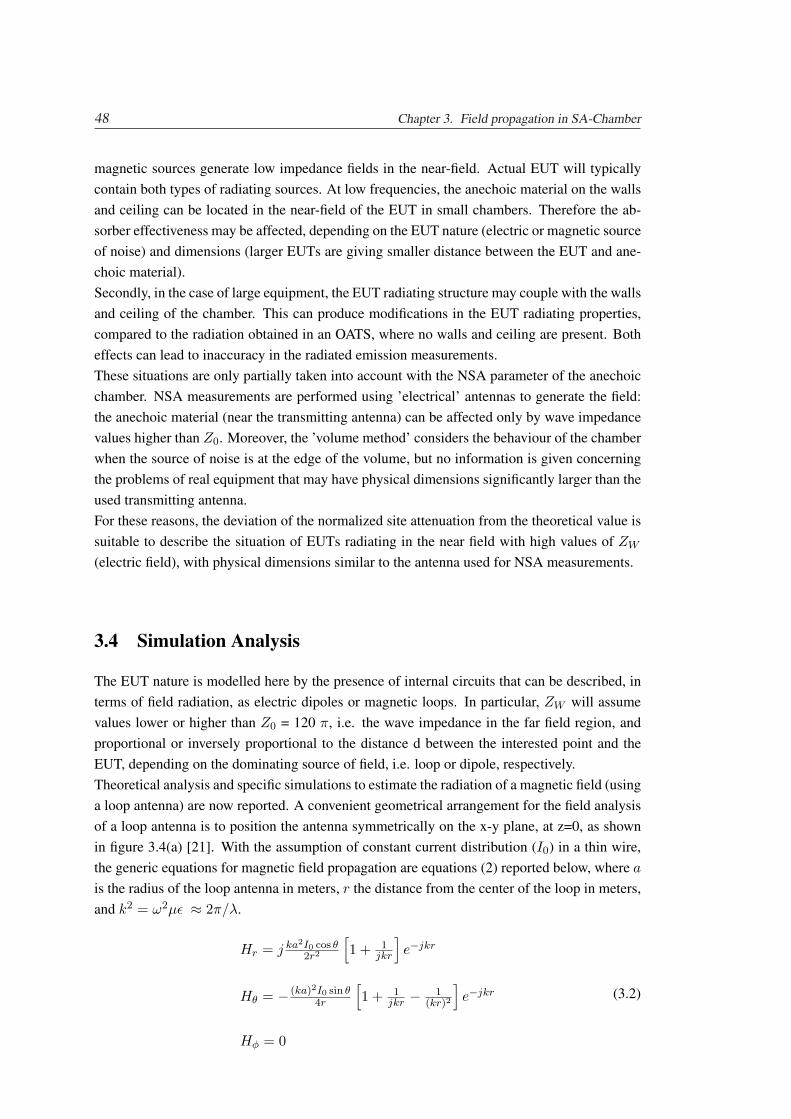
48 Chapter 3. Field propagation in SA-Chamber
magnetic sources generate low impedance fields in the near-field. Actual EUT will typicallycontain both types of radiating sources. At low frequencies, the anechoic material on the wallsand ceiling can be located in the near-field of the EUT in small chambers. Therefore the ab-sorber effectiveness may be affected, depending on the EUT nature (electric or magnetic sourceof noise) and dimensions (larger EUTs are giving smaller distance between the EUT and ane-choic material).Secondly, in the case of large equipment, the EUT radiating structure may couple with the wallsand ceiling of the chamber. This can produce modifications in the EUT radiating properties,compared to the radiation obtained in an OATS, where no walls and ceiling are present. Botheffects can lead to inaccuracy in the radiated emission measurements.These situations are only partially taken into account with the NSA parameter of the anechoicchamber. NSA measurements are performed using ’electrical’ antennas to generate the field:the anechoic material (near the transmitting antenna) can be affected only by wave impedancevalues higher than Z0. Moreover, the ’volume method’ considers the behaviour of the chamberwhen the source of noise is at the edge of the volume, but no information is given concerningthe problems of real equipment that may have physical dimensions significantly larger than theused transmitting antenna.For these reasons, the deviation of the normalized site attenuation from the theoretical value issuitable to describe the situation of EUTs radiating in the near field with high values of ZW
(electric field), with physical dimensions similar to the antenna used for NSA measurements.
3.4 Simulation Analysis
The EUT nature is modelled here by the presence of internal circuits that can be described, interms of field radiation, as electric dipoles or magnetic loops. In particular, ZW will assumevalues lower or higher than Z0 = 120 π, i.e. the wave impedance in the far field region, andproportional or inversely proportional to the distance d between the interested point and theEUT, depending on the dominating source of field, i.e. loop or dipole, respectively.Theoretical analysis and specific simulations to estimate the radiation of a magnetic field (usinga loop antenna) are now reported. A convenient geometrical arrangement for the field analysisof a loop antenna is to position the antenna symmetrically on the x-y plane, at z=0, as shownin figure 3.4(a) [21]. With the assumption of constant current distribution (I0) in a thin wire,the generic equations for magnetic field propagation are equations (2) reported below, where a
is the radius of the loop antenna in meters, r the distance from the center of the loop in meters,and k2 = ω2µε ≈ 2π/λ.
Hr = j ka2I0 cos θ2r2
[1 + 1
jkr
]e−jkr
Hθ = − (ka)2I0 sin θ4r
[1 + 1
jkr − 1(kr)2
]e−jkr
Hφ = 0
(3.2)
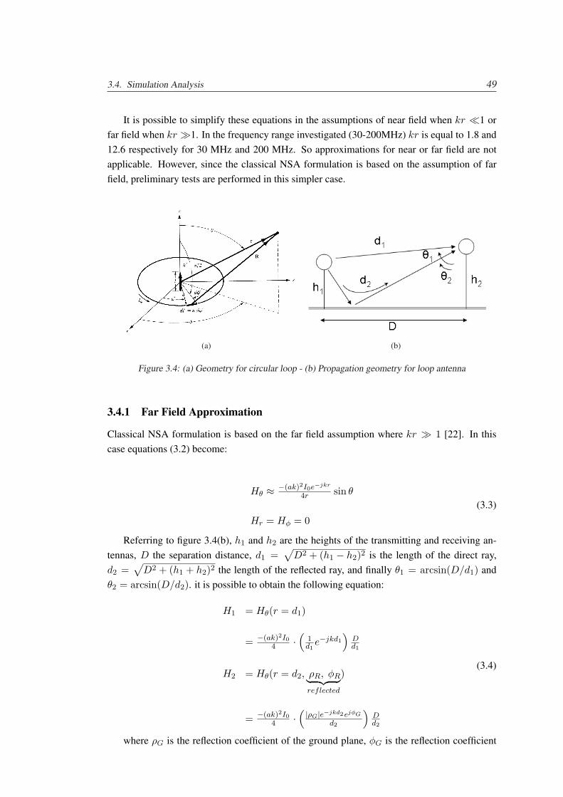
3.4. Simulation Analysis 49
It is possible to simplify these equations in the assumptions of near field when kr ¿1 orfar field when kr À1. In the frequency range investigated (30-200MHz) kr is equal to 1.8 and12.6 respectively for 30 MHz and 200 MHz. So approximations for near or far field are notapplicable. However, since the classical NSA formulation is based on the assumption of farfield, preliminary tests are performed in this simpler case.
(a) (b)
Figure 3.4: (a) Geometry for circular loop - (b) Propagation geometry for loop antenna
3.4.1 Far Field Approximation
Classical NSA formulation is based on the far field assumption where kr À 1 [22]. In thiscase equations (3.2) become:
Hθ ≈ −(ak)2I0e−jkr
4r sin θ
Hr = Hφ = 0
(3.3)
Referring to figure 3.4(b), h1 and h2 are the heights of the transmitting and receiving an-tennas, D the separation distance, d1 =
√D2 + (h1 − h2)2 is the length of the direct ray,
d2 =√
D2 + (h1 + h2)2 the length of the reflected ray, and finally θ1 = arcsin(D/d1) andθ2 = arcsin(D/d2). it is possible to obtain the following equation:
H1 = Hθ(r = d1)
= −(ak)2I04 ·
(1d1
e−jkd1
)Dd1
H2 = Hθ(r = d2, ρR, φR︸ ︷︷ ︸reflected
)
= −(ak)2I04 ·
( |ρG|e−jkd2ejφG
d2
)Dd2
(3.4)
where ρG is the reflection coefficient of the ground plane, φG is the reflection coefficient
50 Chapter 3. Field propagation in SA-Chamber
phase angle; in case of total reflection without phase displacement: ρ = 1 and φ = 0. The totalfield is the algebraic sum of H1 and H2 and final equation is:
HTOT =−(ak)2
4I0D ·
(e−jkd1
d21
+|ρG|e−j(kd2−φG)
d22
)(3.5)
The magnitude of (3.5) is:
|HTOT | = −(ak)2
4I0D ·
√d4
2 + d41|ρG|+ 2(d1d2)2|ρG| cos(φG − k(d2 − d1))
(d1d2)2(3.6)
The electrical size of loop (circumference) determines the efficiency of the loop antenna[21]. Loop antennas are usually classified as either electrically small or electrically large basedon the loop circumference (C). An electrically small loop circumference is less than λ/10,while for an electrically large loop the circumference is ≈ λ/10. For convenience we defineK = C/λ
To maintain a good ’match’ between the circumference of the loop and its working frequencyrange, three different antenna radii have been used: a1= 16 cm for the frequency range 30MHz to 80 MHz, a2= 6 cm for the frequency range 80 MHz to 140 MHz and a3= 3.4 cm forthe frequency range 140 MHz to 200 MHz. Such solutions are shown in table 3.1 where thevalues of K are reported for each antenna in the respective frequency range.
Radius [cm] fmin [MHz] fMAX [MHz] Kmin KMAX
16 30 80 0.1 0.276 80 140 0.1 0.18
3.4 140 200 0.1 0.14
Table 3.1: Loop Diameters
The effects of the variation in radiation patterns with respect to the value K are reportedin figure 3.5. Pictures show the radiation patterns for the best case with C = 0.1λ (K=0.1),assuming a uniform current distribution and for K=0.27. These patterns indicate that the fieldradiated by the loop along its axis (θ=0) is zero. The shape of the propagation is similar in bothcases. Unfortunately this propagation pattern regards the far field case and near field effectsare not accounted for. In the latter case, multiple lobes should appear.Using equation (3.6), predictions of H field radiation with I0 = 500µA, D = 3m, h1 = h2 =1m, are shown in figure 3.6 for the three loops.
3.4.2 Validation of the model
To evaluate the accuracy of the predictions obtained with the simplified equations and alsoto preliminarily investigate the effect of a magnetic field source, the loop antennas previouslydescribed are then used as transmitting devices in their respective working frequency ranges(D = 3 m, h1 = h2 = 1 m). The measurement of the field strength has been carried out by usinga calibrated biconical antenna, so electric field is obtained using the antenna factors. With
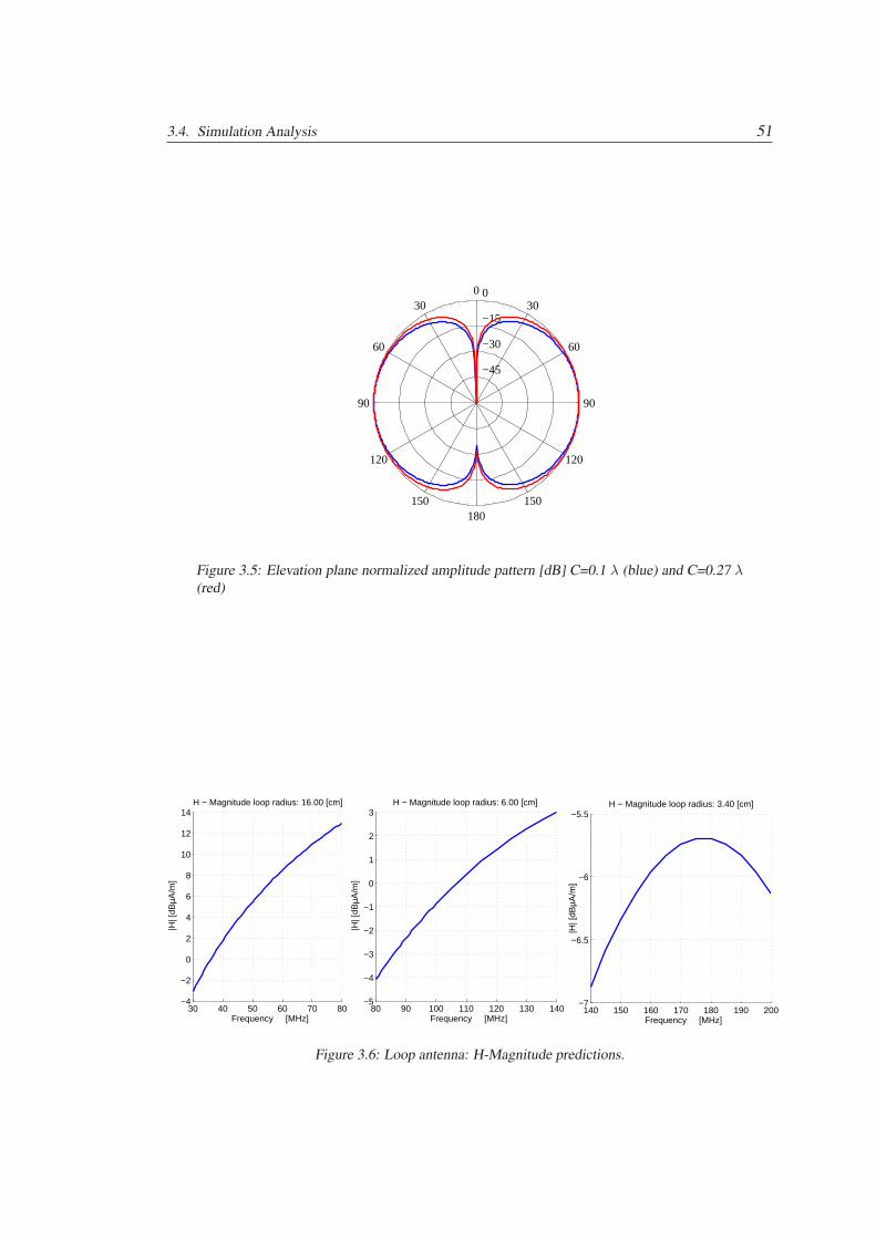
3.4. Simulation Analysis 51
−45
−30
−15
0
60
120
30
150
0
180
30
150
60
120
90 90
Figure 3.5: Elevation plane normalized amplitude pattern [dB] C=0.1 λ (blue) and C=0.27 λ(red)
30 40 50 60 70 80−4
−2
0
2
4
6
8
10
12
14H − Magnitude loop radius: 16.00 [cm]
Frequency [MHz]
|H| [
dBµA
/m]
80 90 100 110 120 130 140−5
−4
−3
−2
−1
0
1
2
3H − Magnitude loop radius: 6.00 [cm]
Frequency [MHz]
|H| [
dBµA
/m]
140 150 160 170 180 190 200−7
−6.5
−6
−5.5H − Magnitude loop radius: 3.40 [cm]
Frequency [MHz]
|H| [
dBµA
/m]
Figure 3.6: Loop antenna: H-Magnitude predictions.
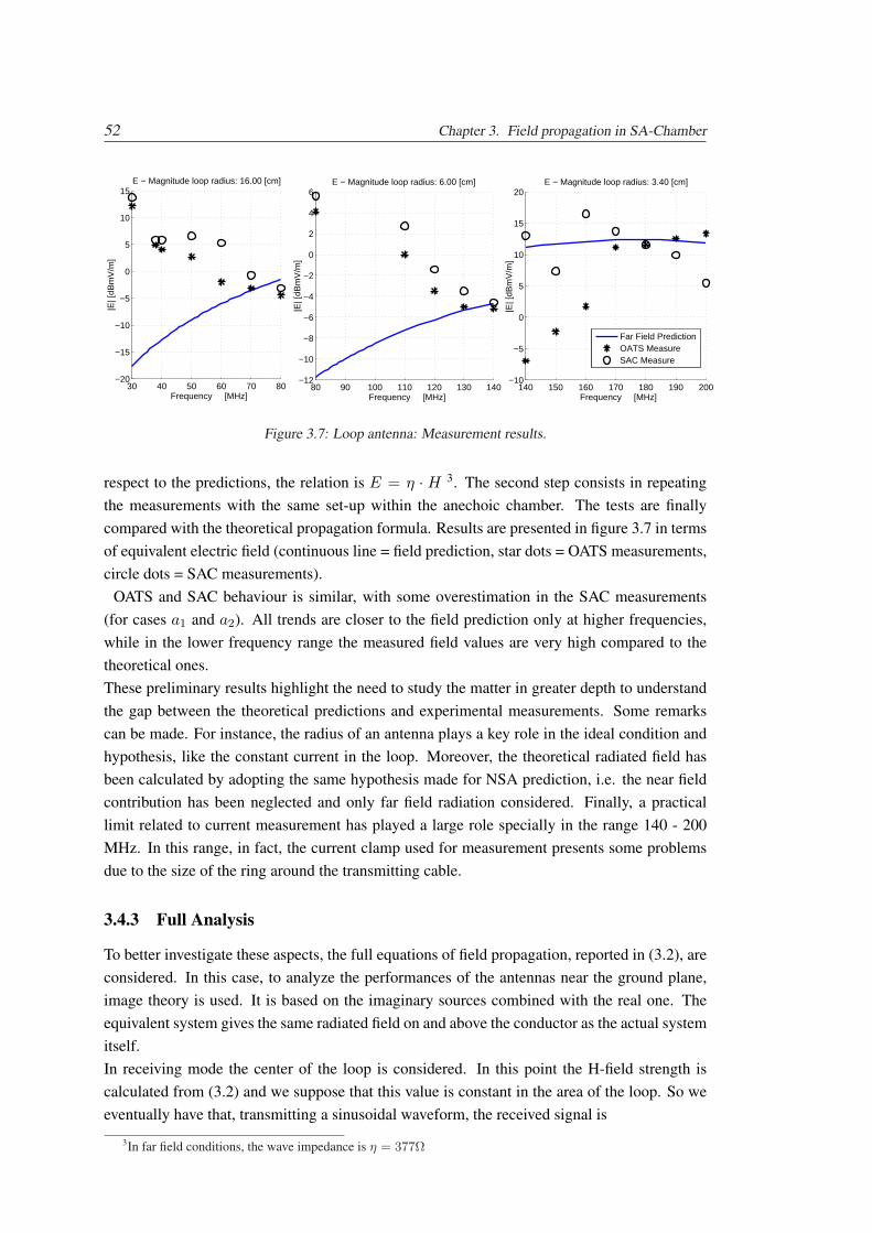
52 Chapter 3. Field propagation in SA-Chamber
30 40 50 60 70 80−20
−15
−10
−5
0
5
10
15E − Magnitude loop radius: 16.00 [cm]
Frequency [MHz]
|E| [
dBm
V/m
]
80 90 100 110 120 130 140−12
−10
−8
−6
−4
−2
0
2
4
6E − Magnitude loop radius: 6.00 [cm]
Frequency [MHz]
|E| [
dBm
V/m
]
140 150 160 170 180 190 200−10
−5
0
5
10
15
20E − Magnitude loop radius: 3.40 [cm]
Frequency [MHz]
|E| [
dBm
V/m
]
Far Field PredictionOATS MeasureSAC Measure
Figure 3.7: Loop antenna: Measurement results.
respect to the predictions, the relation is E = η · H 3. The second step consists in repeatingthe measurements with the same set-up within the anechoic chamber. The tests are finallycompared with the theoretical propagation formula. Results are presented in figure 3.7 in termsof equivalent electric field (continuous line = field prediction, star dots = OATS measurements,circle dots = SAC measurements).
OATS and SAC behaviour is similar, with some overestimation in the SAC measurements(for cases a1 and a2). All trends are closer to the field prediction only at higher frequencies,while in the lower frequency range the measured field values are very high compared to thetheoretical ones.These preliminary results highlight the need to study the matter in greater depth to understandthe gap between the theoretical predictions and experimental measurements. Some remarkscan be made. For instance, the radius of an antenna plays a key role in the ideal condition andhypothesis, like the constant current in the loop. Moreover, the theoretical radiated field hasbeen calculated by adopting the same hypothesis made for NSA prediction, i.e. the near fieldcontribution has been neglected and only far field radiation considered. Finally, a practicallimit related to current measurement has played a large role specially in the range 140 - 200MHz. In this range, in fact, the current clamp used for measurement presents some problemsdue to the size of the ring around the transmitting cable.
3.4.3 Full Analysis
To better investigate these aspects, the full equations of field propagation, reported in (3.2), areconsidered. In this case, to analyze the performances of the antennas near the ground plane,image theory is used. It is based on the imaginary sources combined with the real one. Theequivalent system gives the same radiated field on and above the conductor as the actual systemitself.In receiving mode the center of the loop is considered. In this point the H-field strength iscalculated from (3.2) and we suppose that this value is constant in the area of the loop. So weeventually have that, transmitting a sinusoidal waveform, the received signal is
3In far field conditions, the wave impedance is η = 377Ω
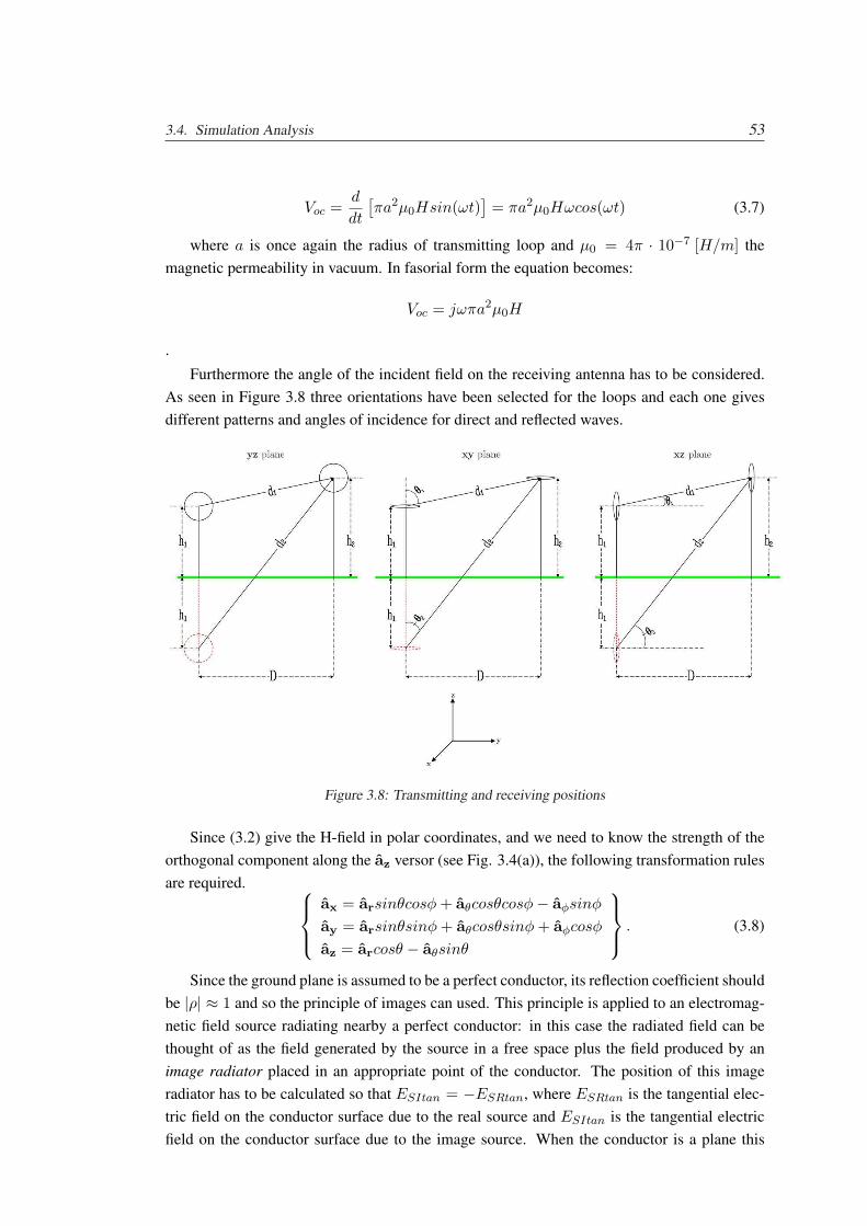
3.4. Simulation Analysis 53
Voc =d
dt
[πa2µ0Hsin(ωt)
]= πa2µ0Hωcos(ωt) (3.7)
where a is once again the radius of transmitting loop and µ0 = 4π · 10−7 [H/m] themagnetic permeability in vacuum. In fasorial form the equation becomes:
Voc = jωπa2µ0H
.
Furthermore the angle of the incident field on the receiving antenna has to be considered.As seen in Figure 3.8 three orientations have been selected for the loops and each one givesdifferent patterns and angles of incidence for direct and reflected waves.
Figure 3.8: Transmitting and receiving positions
Since (3.2) give the H-field in polar coordinates, and we need to know the strength of theorthogonal component along the az versor (see Fig. 3.4(a)), the following transformation rulesare required.
ax = arsinθcosφ + aθcosθcosφ− aφsinφ
ay = arsinθsinφ + aθcosθsinφ + aφcosφ
az = arcosθ − aθsinθ
. (3.8)
Since the ground plane is assumed to be a perfect conductor, its reflection coefficient shouldbe |ρ| ≈ 1 and so the principle of images can used. This principle is applied to an electromag-netic field source radiating nearby a perfect conductor: in this case the radiated field can bethought of as the field generated by the source in a free space plus the field produced by animage radiator placed in an appropriate point of the conductor. The position of this imageradiator has to be calculated so that ESItan = −ESRtan, where ESRtan is the tangential elec-tric field on the conductor surface due to the real source and ESItan is the tangential electricfield on the conductor surface due to the image source. When the conductor is a plane this
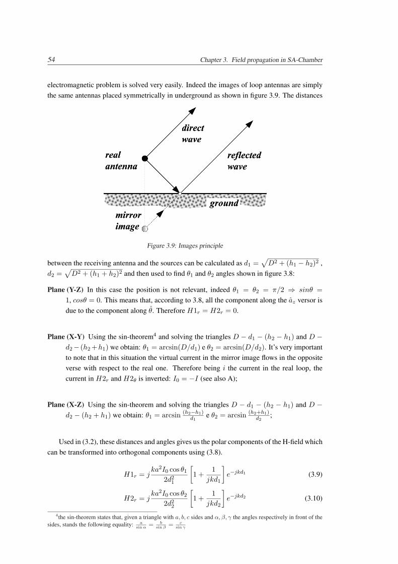
54 Chapter 3. Field propagation in SA-Chamber
electromagnetic problem is solved very easily. Indeed the images of loop antennas are simplythe same antennas placed symmetrically in underground as shown in figure 3.9. The distances
Figure 3.9: Images principle
between the receiving antenna and the sources can be calculated as d1 =√
D2 + (h1 − h2)2 ,d2 =
√D2 + (h1 + h2)2 and then used to find θ1 and θ2 angles shown in figure 3.8:
Plane (Y-Z) In this case the position is not relevant, indeed θ1 = θ2 = π/2 ⇒ sinθ =1, cosθ = 0. This means that, according to 3.8, all the component along the az versor isdue to the component along θ. Therefore H1r = H2r = 0.
Plane (X-Y) Using the sin-theorem4 and solving the triangles D − d1 − (h2 − h1) and D −d2− (h2 +h1) we obtain: θ1 = arcsin(D/d1) e θ2 = arcsin(D/d2). It’s very importantto note that in this situation the virtual current in the mirror image flows in the oppositeverse with respect to the real one. Therefore being i the current in the real loop, thecurrent in H2r and H2θ is inverted: I0 = −I (see also A);
Plane (X-Z) Using the sin-theorem and solving the triangles D − d1 − (h2 − h1) and D −d2 − (h2 + h1) we obtain: θ1 = arcsin (h2−h1)
d1e θ2 = arcsin (h2+h1)
d2;
Used in (3.2), these distances and angles gives us the polar components of the H-field whichcan be transformed into orthogonal components using (3.8).
H1r = jka2I0 cos θ1
2d21
[1 +
1jkd1
]e−jkd1 (3.9)
H2r = jka2I0 cos θ2
2d22
[1 +
1jkd2
]e−jkd2 (3.10)
4the sin-theorem states that, given a triangle with a, b, c sides and α, β, γ the angles respectively in front of thesides, stands the following equality: a
sin α= b
sin β= c
sin γ
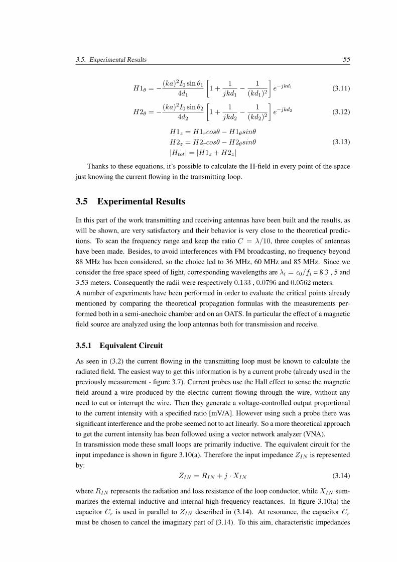
3.5. Experimental Results 55
H1θ = −(ka)2I0 sin θ1
4d1
[1 +
1jkd1
− 1(kd1)2
]e−jkd1 (3.11)
H2θ = −(ka)2I0 sin θ2
4d2
[1 +
1jkd2
− 1(kd2)2
]e−jkd2 (3.12)
H1z = H1rcosθ −H1θsinθ
H2z = H2rcosθ −H2θsinθ
|Htot| = |H1z + H2z|(3.13)
Thanks to these equations, it’s possible to calculate the H-field in every point of the spacejust knowing the current flowing in the transmitting loop.
3.5 Experimental Results
In this part of the work transmitting and receiving antennas have been built and the results, aswill be shown, are very satisfactory and their behavior is very close to the theoretical predic-tions. To scan the frequency range and keep the ratio C = λ/10, three couples of antennashave been made. Besides, to avoid interferences with FM broadcasting, no frequency beyond88 MHz has been considered, so the choice led to 36 MHz, 60 MHz and 85 MHz. Since weconsider the free space speed of light, corresponding wavelengths are λi = c0/fi = 8.3 , 5 and3.53 meters. Consequently the radii were respectively 0.133 , 0.0796 and 0.0562 meters.A number of experiments have been performed in order to evaluate the critical points alreadymentioned by comparing the theoretical propagation formulas with the measurements per-formed both in a semi-anechoic chamber and on an OATS. In particular the effect of a magneticfield source are analyzed using the loop antennas both for transmission and receive.
3.5.1 Equivalent Circuit
As seen in (3.2) the current flowing in the transmitting loop must be known to calculate theradiated field. The easiest way to get this information is by a current probe (already used in thepreviously measurement - figure 3.7). Current probes use the Hall effect to sense the magneticfield around a wire produced by the electric current flowing through the wire, without anyneed to cut or interrupt the wire. Then they generate a voltage-controlled output proportionalto the current intensity with a specified ratio [mV/A]. However using such a probe there wassignificant interference and the probe seemed not to act linearly. So a more theoretical approachto get the current intensity has been followed using a vector network analyzer (VNA).In transmission mode these small loops are primarily inductive. The equivalent circuit for theinput impedance is shown in figure 3.10(a). Therefore the input impedance ZIN is representedby:
ZIN = RIN + j ·XIN (3.14)
where RIN represents the radiation and loss resistance of the loop conductor, while XIN sum-marizes the external inductive and internal high-frequency reactances. In figure 3.10(a) thecapacitor Cr is used in parallel to ZIN described in (3.14). At resonance, the capacitor Cr
must be chosen to cancel the imaginary part of (3.14). To this aim, characteristic impedances
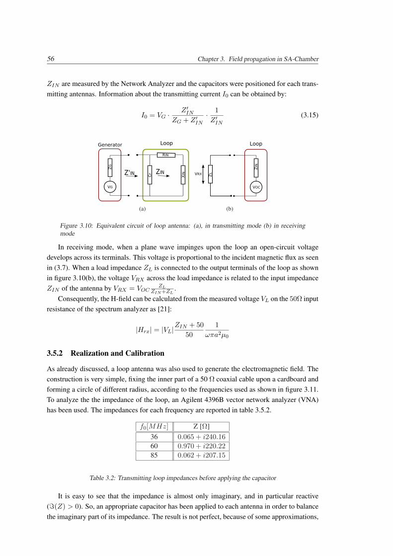
56 Chapter 3. Field propagation in SA-Chamber
ZIN are measured by the Network Analyzer and the capacitors were positioned for each trans-mitting antennas. Information about the transmitting current I0 can be obtained by:
I0 = VG · Z ′IN
ZG + Z ′IN
· 1Z ′IN
(3.15)
(a) (b)
Figure 3.10: Equivalent circuit of loop antenna: (a), in transmitting mode (b) in receivingmode
In receiving mode, when a plane wave impinges upon the loop an open-circuit voltagedevelops across its terminals. This voltage is proportional to the incident magnetic flux as seenin (3.7). When a load impedance ZL is connected to the output terminals of the loop as shownin figure 3.10(b), the voltage VRX across the load impedance is related to the input impedanceZIN of the antenna by VRX = VOC
ZLZIN+ZL
.Consequently, the H-field can be calculated from the measured voltage VL on the 50Ω input
resistance of the spectrum analyzer as [21]:
|Hrx| = |VL|ZIN + 5050
1ωπa2µ0
3.5.2 Realization and Calibration
As already discussed, a loop antenna was also used to generate the electromagnetic field. Theconstruction is very simple, fixing the inner part of a 50 Ω coaxial cable upon a cardboard andforming a circle of different radius, according to the frequencies used as shown in figure 3.11.To analyze the the impedance of the loop, an Agilent 4396B vector network analyzer (VNA)has been used. The impedances for each frequency are reported in table 3.5.2.
f0[MHz] Z [Ω]36 0.065 + i240.1660 0.970 + i220.2285 0.062 + i207.15
Table 3.2: Transmitting loop impedances before applying the capacitor
It is easy to see that the impedance is almost only imaginary, and in particular reactive(=(Z) > 0). So, an appropriate capacitor has been applied to each antenna in order to balancethe imaginary part of its impedance. The result is not perfect, because of some approximations,
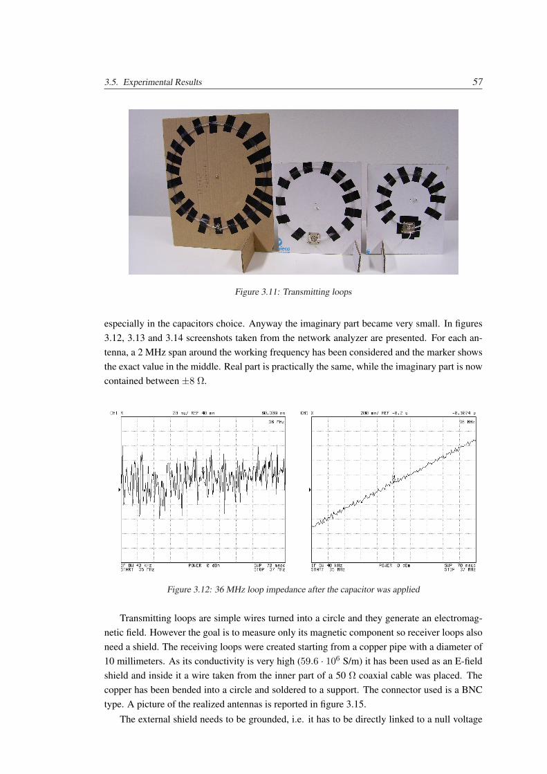
3.5. Experimental Results 57
Figure 3.11: Transmitting loops
especially in the capacitors choice. Anyway the imaginary part became very small. In figures3.12, 3.13 and 3.14 screenshots taken from the network analyzer are presented. For each an-tenna, a 2 MHz span around the working frequency has been considered and the marker showsthe exact value in the middle. Real part is practically the same, while the imaginary part is nowcontained between ±8 Ω.
Figure 3.12: 36 MHz loop impedance after the capacitor was applied
Transmitting loops are simple wires turned into a circle and they generate an electromag-netic field. However the goal is to measure only its magnetic component so receiver loops alsoneed a shield. The receiving loops were created starting from a copper pipe with a diameter of10 millimeters. As its conductivity is very high (59.6 · 106 S/m) it has been used as an E-fieldshield and inside it a wire taken from the inner part of a 50 Ω coaxial cable was placed. Thecopper has been bended into a circle and soldered to a support. The connector used is a BNCtype. A picture of the realized antennas is reported in figure 3.15.
The external shield needs to be grounded, i.e. it has to be directly linked to a null voltage
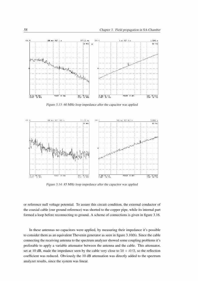
58 Chapter 3. Field propagation in SA-Chamber
Figure 3.13: 60 MHz loop impedance after the capacitor was applied
Figure 3.14: 85 MHz loop impedance after the capacitor was applied
or reference null voltage potential. To assure this circuit condition, the external conductor ofthe coaxial cable (our ground reference) was shorted to the copper pipe, while its internal partformed a loop before reconnecting to ground. A scheme of connections is given in figure 3.16.
In these antennas no capacitors were applied, by measuring their impedance it’s possibleto consider them as an equivalent Thevenin generator as seen in figure 3.10(b). Since the cableconnecting the receiving antenna to the spectrum analyzer showed some coupling problems it’spreferable to apply a variable attenuator between the antenna and the cable. This attenuator,set at 10 dB, made the impedance seen by the cable very close to 50 + i0 Ω, so the reflectioncoefficient was reduced. Obviously the 10 dB attenuation was directly added to the spectrumanalyzer results, since the system was linear.
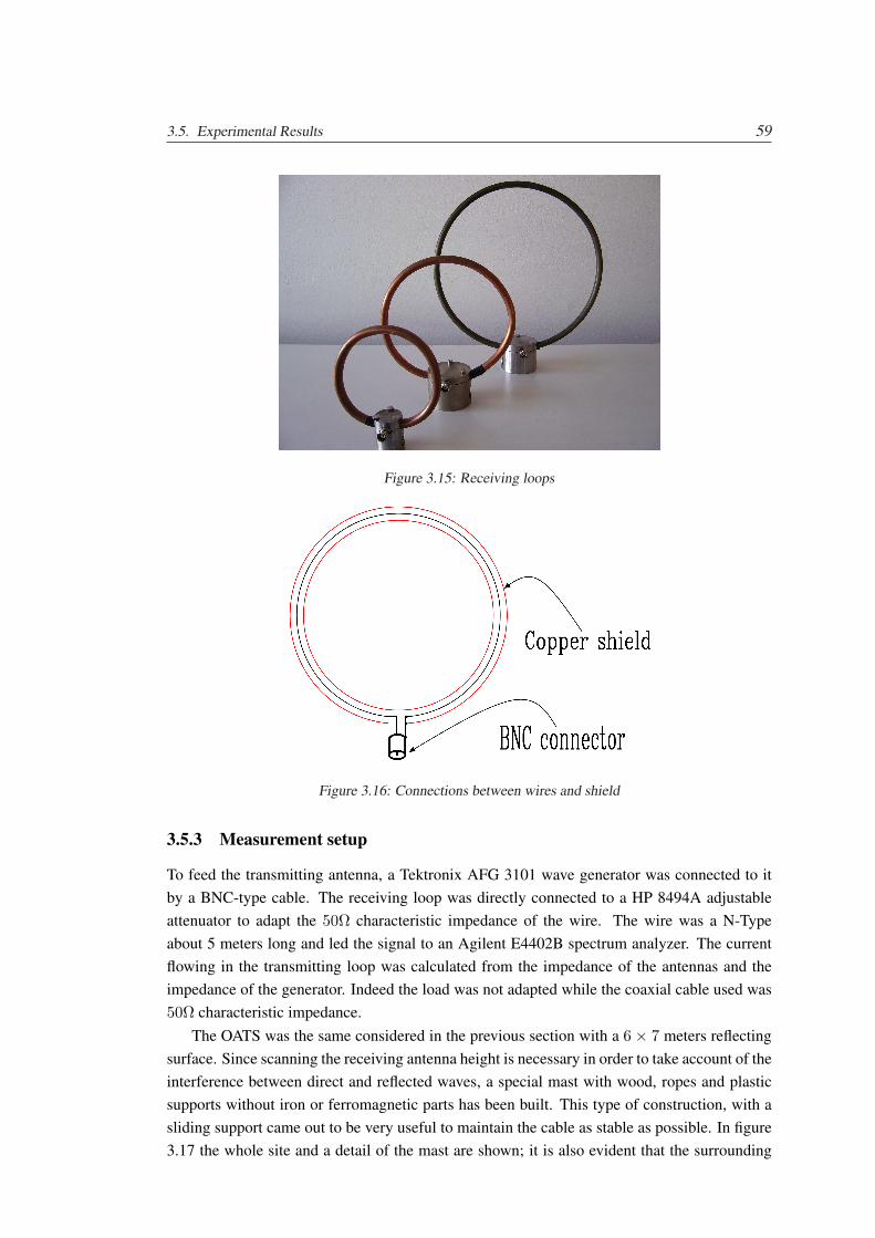
3.5. Experimental Results 59
Figure 3.15: Receiving loops
Figure 3.16: Connections between wires and shield
3.5.3 Measurement setup
To feed the transmitting antenna, a Tektronix AFG 3101 wave generator was connected to itby a BNC-type cable. The receiving loop was directly connected to a HP 8494A adjustableattenuator to adapt the 50Ω characteristic impedance of the wire. The wire was a N-Typeabout 5 meters long and led the signal to an Agilent E4402B spectrum analyzer. The currentflowing in the transmitting loop was calculated from the impedance of the antennas and theimpedance of the generator. Indeed the load was not adapted while the coaxial cable used was50Ω characteristic impedance.
The OATS was the same considered in the previous section with a 6 × 7 meters reflectingsurface. Since scanning the receiving antenna height is necessary in order to take account of theinterference between direct and reflected waves, a special mast with wood, ropes and plasticsupports without iron or ferromagnetic parts has been built. This type of construction, with asliding support came out to be very useful to maintain the cable as stable as possible. In figure3.17 the whole site and a detail of the mast are shown; it is also evident that the surrounding
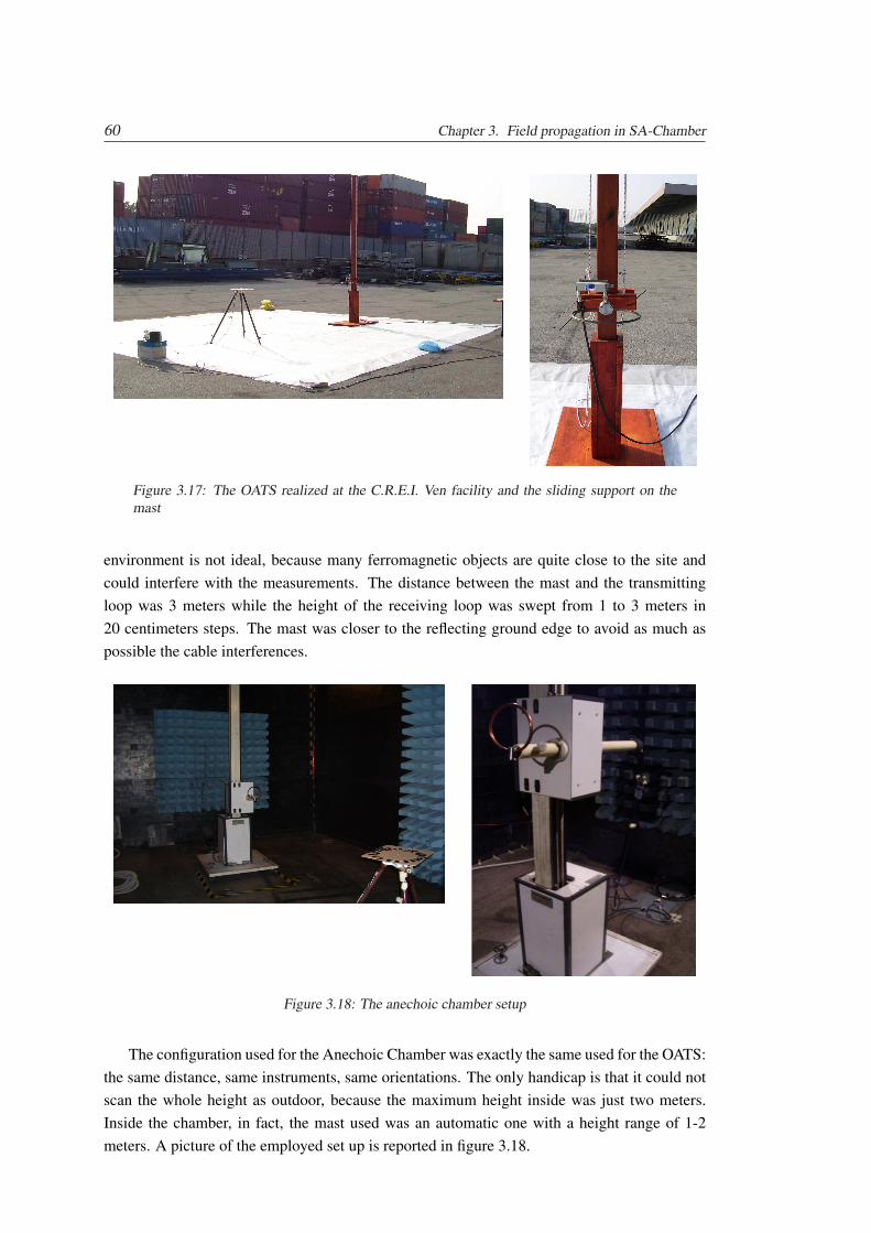
60 Chapter 3. Field propagation in SA-Chamber
Figure 3.17: The OATS realized at the C.R.E.I. Ven facility and the sliding support on themast
environment is not ideal, because many ferromagnetic objects are quite close to the site andcould interfere with the measurements. The distance between the mast and the transmittingloop was 3 meters while the height of the receiving loop was swept from 1 to 3 meters in20 centimeters steps. The mast was closer to the reflecting ground edge to avoid as much aspossible the cable interferences.
Figure 3.18: The anechoic chamber setup
The configuration used for the Anechoic Chamber was exactly the same used for the OATS:the same distance, same instruments, same orientations. The only handicap is that it could notscan the whole height as outdoor, because the maximum height inside was just two meters.Inside the chamber, in fact, the mast used was an automatic one with a height range of 1-2meters. A picture of the employed set up is reported in figure 3.18.
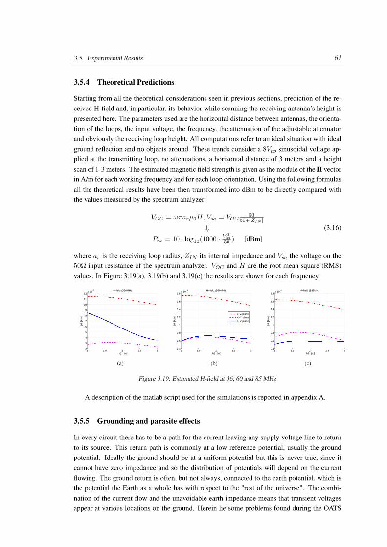
3.5. Experimental Results 61
3.5.4 Theoretical Predictions
Starting from all the theoretical considerations seen in previous sections, prediction of the re-ceived H-field and, in particular, its behavior while scanning the receiving antenna’s height ispresented here. The parameters used are the horizontal distance between antennas, the orienta-tion of the loops, the input voltage, the frequency, the attenuation of the adjustable attenuatorand obviously the receiving loop height. All computations refer to an ideal situation with idealground reflection and no objects around. These trends consider a 8Vpp sinusoidal voltage ap-plied at the transmitting loop, no attenuations, a horizontal distance of 3 meters and a heightscan of 1-3 meters. The estimated magnetic field strength is given as the module of the H vectorin A/m for each working frequency and for each loop orientation. Using the following formulasall the theoretical results have been then transformed into dBm to be directly compared withthe values measured by the spectrum analyzer:
VOC = ωπarµ0H , Vsa = VOC50
50+|ZIN |⇓
Prx = 10 · log10(1000 · V 2sa50 ) [dBm]
(3.16)
where ar is the receiving loop radius, ZIN its internal impedance and Vsa the voltage on the50Ω input resistance of the spectrum analyzer. VOC and H are the root mean square (RMS)values. In Figure 3.19(a), 3.19(b) and 3.19(c) the results are shown for each frequency.
1 1.5 2 2.5 32
3
4
5
6
7
8
9
10
11
12x 10
−5 H−field @36MHz
h2 [m]
|H| [
A/m
]
(a)
1 1.5 2 2.5 30.4
0.6
0.8
1
1.2
1.4
1.6
1.8x 10
−4 H−field @60MHz
h2 [m]
|H| [
A/m
]
Y−Z planeX−Y planeX−Z plane
(b)
1 1.5 2 2.5 30.4
0.6
0.8
1
1.2
1.4
1.6
1.8x 10
−4 H−field @85MHz
h2 [m]
|H| [
A/m
]
(c)
Figure 3.19: Estimated H-field at 36, 60 and 85 MHz
A description of the matlab script used for the simulations is reported in appendix A.
3.5.5 Grounding and parasite effects
In every circuit there has to be a path for the current leaving any supply voltage line to returnto its source. This return path is commonly at a low reference potential, usually the groundpotential. Ideally the ground should be at a uniform potential but this is never true, since itcannot have zero impedance and so the distribution of potentials will depend on the currentflowing. The ground return is often, but not always, connected to the earth potential, which isthe potential the Earth as a whole has with respect to the "rest of the universe". The combi-nation of the current flow and the unavoidable earth impedance means that transient voltagesappear at various locations on the ground. Herein lie some problems found during the OATS
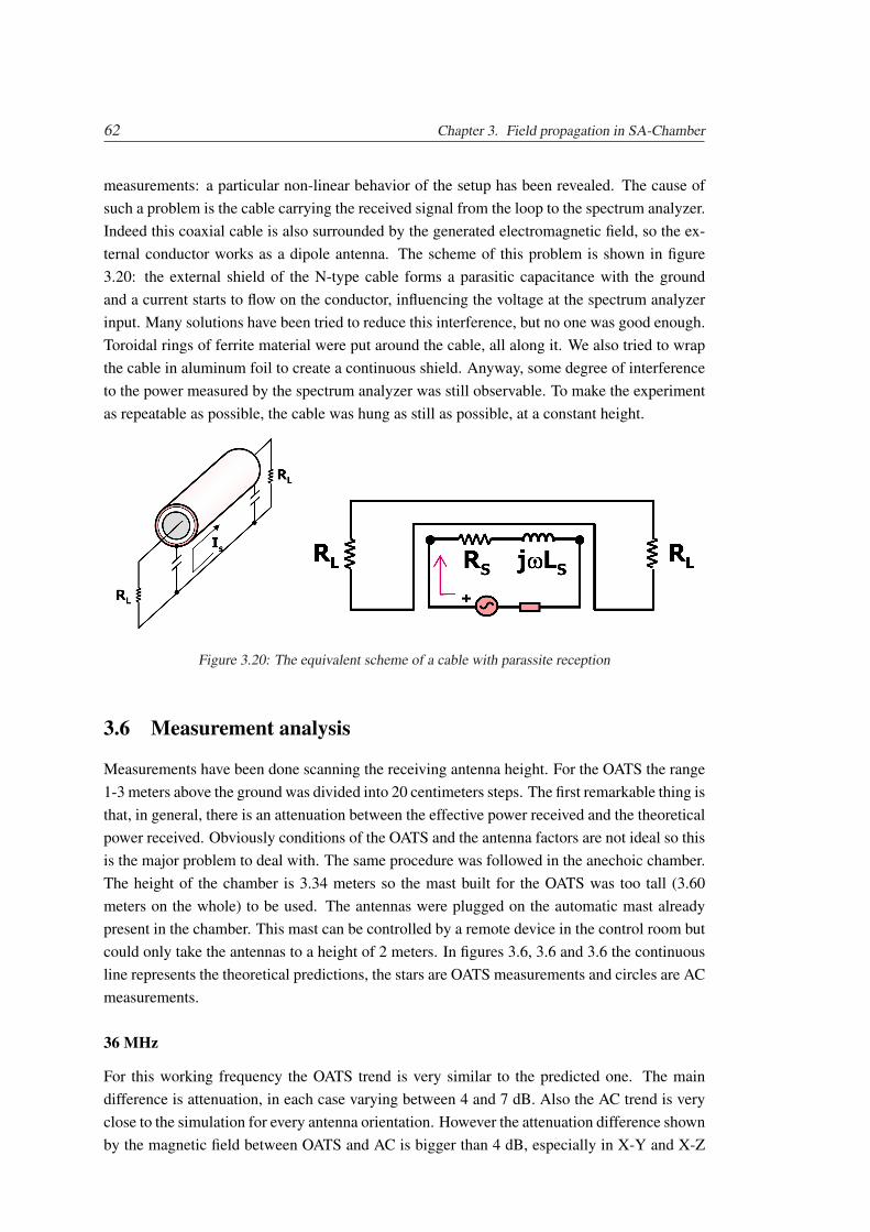
62 Chapter 3. Field propagation in SA-Chamber
measurements: a particular non-linear behavior of the setup has been revealed. The cause ofsuch a problem is the cable carrying the received signal from the loop to the spectrum analyzer.Indeed this coaxial cable is also surrounded by the generated electromagnetic field, so the ex-ternal conductor works as a dipole antenna. The scheme of this problem is shown in figure3.20: the external shield of the N-type cable forms a parasitic capacitance with the groundand a current starts to flow on the conductor, influencing the voltage at the spectrum analyzerinput. Many solutions have been tried to reduce this interference, but no one was good enough.Toroidal rings of ferrite material were put around the cable, all along it. We also tried to wrapthe cable in aluminum foil to create a continuous shield. Anyway, some degree of interferenceto the power measured by the spectrum analyzer was still observable. To make the experimentas repeatable as possible, the cable was hung as still as possible, at a constant height.
Figure 3.20: The equivalent scheme of a cable with parassite reception
3.6 Measurement analysis
Measurements have been done scanning the receiving antenna height. For the OATS the range1-3 meters above the ground was divided into 20 centimeters steps. The first remarkable thing isthat, in general, there is an attenuation between the effective power received and the theoreticalpower received. Obviously conditions of the OATS and the antenna factors are not ideal so thisis the major problem to deal with. The same procedure was followed in the anechoic chamber.The height of the chamber is 3.34 meters so the mast built for the OATS was too tall (3.60meters on the whole) to be used. The antennas were plugged on the automatic mast alreadypresent in the chamber. This mast can be controlled by a remote device in the control room butcould only take the antennas to a height of 2 meters. In figures 3.6, 3.6 and 3.6 the continuousline represents the theoretical predictions, the stars are OATS measurements and circles are ACmeasurements.
36 MHz
For this working frequency the OATS trend is very similar to the predicted one. The maindifference is attenuation, in each case varying between 4 and 7 dB. Also the AC trend is veryclose to the simulation for every antenna orientation. However the attenuation difference shownby the magnetic field between OATS and AC is bigger than 4 dB, especially in X-Y and X-Z
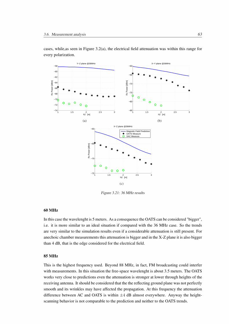
3.6. Measurement analysis 63
cases, while,as seen in Figure 3.2(a), the electrical field attenuation was within this range forevery polarization.
1 1.5 2 2.5 3−74
−72
−70
−68
−66
−64
−62
−60
−58Y−Z plane @36MHz
h2 [m]
Rx
Pow
er [d
Bm
]
(a)
1 1.5 2 2.5 3−85
−80
−75
−70
−65
−60X−Y plane @36MHz
h2 [m]
Rx
Pow
er [d
Bm
]
(b)
1 1.5 2 2.5 3−75
−70
−65
−60X−Z plane @36MHz
h2 [m]
Rx
Pow
er [d
Bm
]
Magnetic Field PredictionOATS MeasureSAC Measure
(c)
Figure 3.21: 36 MHz results
60 MHz
In this case the wavelenght is 5 meters. As a consequence the OATS can be considered "bigger",i.e. it is more similar to an ideal situation if compared with the 36 MHz case. So the trendsare very similar to the simulation results even if a considerable attenuation is still present. Foranechoic chamber measurements this attenuation is bigger and in the X-Z plane it is also biggerthan 4 dB, that is the edge considered for the electrical field.
85 MHz
This is the highest frequency used. Beyond 88 MHz, in fact, FM broadcasting could interferwith measurements. In this situation the free-space wavelenght is about 3.5 meters. The OATSworks very close to predictions even the attenuation is stronger at lower through heights of thereceiving antenna. It should be considered that the the reflecting ground plane was not perfectlysmooth and its wrinkles may have affected the propagation. At this frequency the attenuationdifference between AC and OATS is within ±4 dB almost everywhere. Anyway the height-scanning behavior is not comparable to the prediction and neither to the OATS trends.
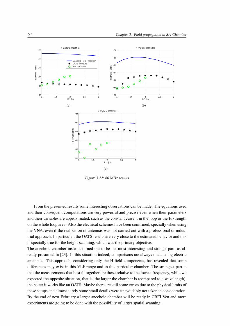
64 Chapter 3. Field propagation in SA-Chamber
1 1.5 2 2.5 3−75
−70
−65
−60
−55
−50Y−Z plane @60MHz
h2 [m]
Rx
Pow
er [d
Bm
]
Magnetic Field PredictionOATS MeasureSAC Measure
(a)
1 1.5 2 2.5 3−70
−68
−66
−64
−62
−60
−58X−Y plane @60MHz
h2 [m]
Rx
Pow
er [d
Bm
]
(b)
1 1.5 2 2.5 3−80
−75
−70
−65
−60
−55X−Z plane @60MHz
h2 [m]
Rx
Pow
er [d
Bm
]
(c)
Figure 3.22: 60 MHz results
From the presented results some interesting observations can be made. The equations usedand their consequent computations are very powerful and precise even when their parametersand their variables are approximated, such as the constant current in the loop or the H strengthon the whole loop area. Also the electrical schemes have been confirmed, specially when usingthe VNA, even if the realization of antennas was not carried out with a professional or indus-trial approach. In particular, the OATS results are very close to the estimated behavior and thisis specially true for the height-scanning, which was the primary objective.The anechoic chamber instead, turned out to be the most interesting and strange part, as al-ready presumed in [23]. In this situation indeed, comparisons are always made using electricantennas. This approach, considering only the H-field components, has revealed that somedifferences may exist in this VLF range and in this particular chamber. The strangest part isthat the measurements that best fit together are those relative to the lowest frequency, while weexpected the opposite situation, that is, the larger the chamber is (compared to a wavelength),the better it works like an OATS. Maybe there are still some errors due to the physical limits ofthese setups and almost surely some small details were unavoidably not taken in consideration.By the end of next February a larger anechoic chamber will be ready in CREI Ven and moreexperiments are going to be done with the possibility of larger spatial scanning.
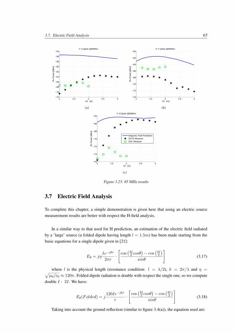
3.7. Electric Field Analysis 65
1 1.5 2 2.5 3−72
−70
−68
−66
−64
−62
−60
−58
−56
−54Y−Z plane @85MHz
h2 [m]
Rx
Pow
er [d
Bm
]
(a)
1 1.5 2 2.5 3−74
−72
−70
−68
−66
−64
−62
−60X−Y plane @85MHz
h2 [m]
Rx
Pow
er [d
Bm
]
(b)
1 1.5 2 2.5 3−76
−74
−72
−70
−68
−66
−64X−Z plane @85MHz
h2 [m]
Rx
Pow
er [d
Bm
]
Magnetic Field PredictionOATS MeasureSAC Measure
(c)
Figure 3.23: 85 MHz results
3.7 Electric Field Analysis
To complete this chapter, a simple demonstration is given here that using an electric sourcemeasurement results are better with respect the H-field analysis.
In a similar way to that used for H prediction, an estimation of the electric field radiatedby a ’large’ source (a folded dipole having length l = 1.5m) has been made starting from thebasic equations for a single dipole given in [21]:
Eθ = jηIe−jkr
2πr·[
cos(
kl2 cosθ
)− cos(
kl2
)
sinθ
](3.17)
where l is the physical length (resonance condition: l = λ/2), k = 2π/λ and η =√µ0/ε0 ≈ 120π. Folded dipole radiation is double with respect the single one, so we compute
double I : 2I . We have:
Eθ(Folded) = j120Ie−jkr
r·[
cos(
kl2 cosθ
)− cos(
kl2
)
sinθ
](3.18)
Taking into account the ground reflection (similar to figure 3.4(a)), the equation used are:
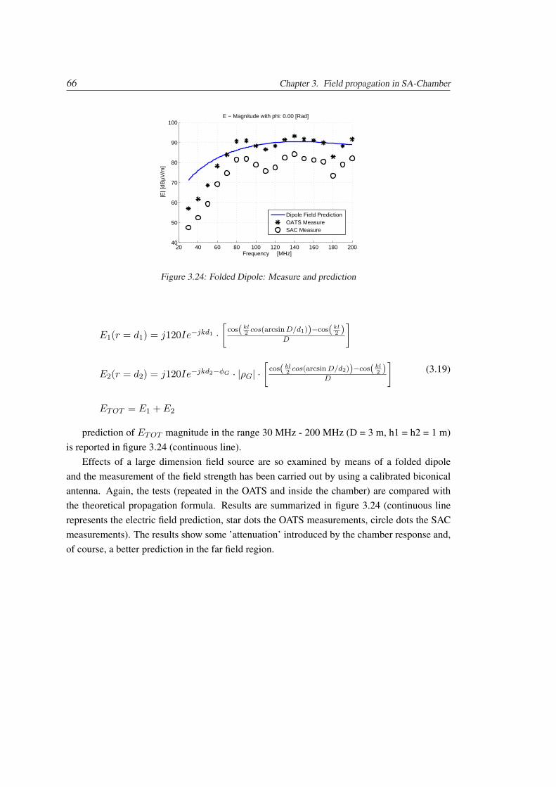
66 Chapter 3. Field propagation in SA-Chamber
20 40 60 80 100 120 140 160 180 20040
50
60
70
80
90
100E − Magnitude with phi: 0.00 [Rad]
Frequency [MHz]
|E| [
dBµV
/m]
Dipole Field PredictionOATS MeasureSAC Measure
Figure 3.24: Folded Dipole: Measure and prediction
E1(r = d1) = j120Ie−jkd1 ·[
cos( kl2
cos(arcsin D/d1))−cos( kl2 )
D
]
E2(r = d2) = j120Ie−jkd2−φG · |ρG| ·[
cos( kl2
cos(arcsin D/d2))−cos( kl2 )
D
]
ETOT = E1 + E2
(3.19)
prediction of ETOT magnitude in the range 30 MHz - 200 MHz (D = 3 m, h1 = h2 = 1 m)is reported in figure 3.24 (continuous line).
Effects of a large dimension field source are so examined by means of a folded dipoleand the measurement of the field strength has been carried out by using a calibrated biconicalantenna. Again, the tests (repeated in the OATS and inside the chamber) are compared withthe theoretical propagation formula. Results are summarized in figure 3.24 (continuous linerepresents the electric field prediction, star dots the OATS measurements, circle dots the SACmeasurements). The results show some ’attenuation’ introduced by the chamber response and,of course, a better prediction in the far field region.
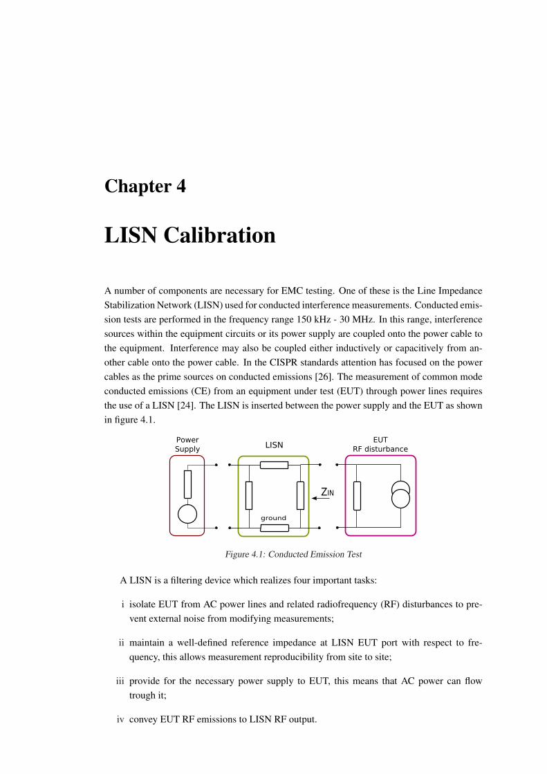
Chapter 4
LISN Calibration
A number of components are necessary for EMC testing. One of these is the Line ImpedanceStabilization Network (LISN) used for conducted interference measurements. Conducted emis-sion tests are performed in the frequency range 150 kHz - 30 MHz. In this range, interferencesources within the equipment circuits or its power supply are coupled onto the power cable tothe equipment. Interference may also be coupled either inductively or capacitively from an-other cable onto the power cable. In the CISPR standards attention has focused on the powercables as the prime sources on conducted emissions [26]. The measurement of common modeconducted emissions (CE) from an equipment under test (EUT) through power lines requiresthe use of a LISN [24]. The LISN is inserted between the power supply and the EUT as shownin figure 4.1.
Figure 4.1: Conducted Emission Test
A LISN is a filtering device which realizes four important tasks:
i isolate EUT from AC power lines and related radiofrequency (RF) disturbances to pre-vent external noise from modifying measurements;
ii maintain a well-defined reference impedance at LISN EUT port with respect to fre-quency, this allows measurement reproducibility from site to site;
iii provide for the necessary power supply to EUT, this means that AC power can flowtrough it;
iv convey EUT RF emissions to LISN RF output.
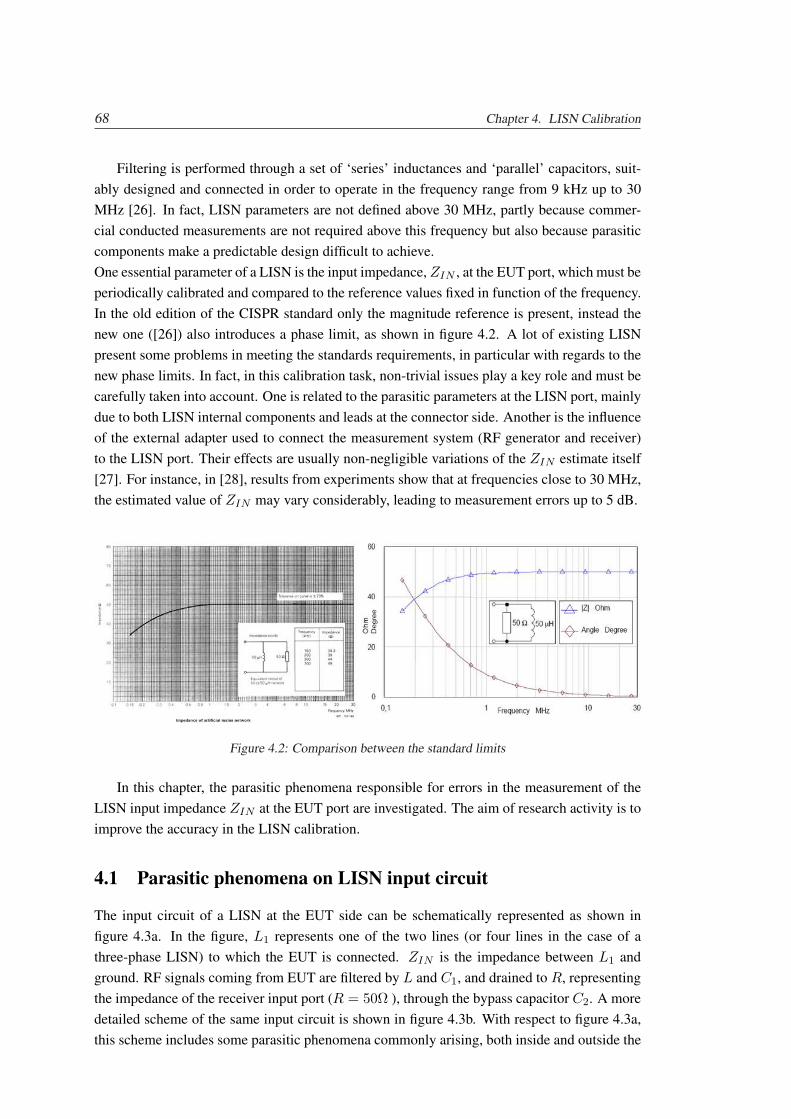
68 Chapter 4. LISN Calibration
Filtering is performed through a set of ‘series’ inductances and ‘parallel’ capacitors, suit-ably designed and connected in order to operate in the frequency range from 9 kHz up to 30MHz [26]. In fact, LISN parameters are not defined above 30 MHz, partly because commer-cial conducted measurements are not required above this frequency but also because parasiticcomponents make a predictable design difficult to achieve.One essential parameter of a LISN is the input impedance, ZIN , at the EUT port, which must beperiodically calibrated and compared to the reference values fixed in function of the frequency.In the old edition of the CISPR standard only the magnitude reference is present, instead thenew one ([26]) also introduces a phase limit, as shown in figure 4.2. A lot of existing LISNpresent some problems in meeting the standards requirements, in particular with regards to thenew phase limits. In fact, in this calibration task, non-trivial issues play a key role and must becarefully taken into account. One is related to the parasitic parameters at the LISN port, mainlydue to both LISN internal components and leads at the connector side. Another is the influenceof the external adapter used to connect the measurement system (RF generator and receiver)to the LISN port. Their effects are usually non-negligible variations of the ZIN estimate itself[27]. For instance, in [28], results from experiments show that at frequencies close to 30 MHz,the estimated value of ZIN may vary considerably, leading to measurement errors up to 5 dB.
Figure 4.2: Comparison between the standard limits
In this chapter, the parasitic phenomena responsible for errors in the measurement of theLISN input impedance ZIN at the EUT port are investigated. The aim of research activity is toimprove the accuracy in the LISN calibration.
4.1 Parasitic phenomena on LISN input circuit
The input circuit of a LISN at the EUT side can be schematically represented as shown infigure 4.3a. In the figure, L1 represents one of the two lines (or four lines in the case of athree-phase LISN) to which the EUT is connected. ZIN is the impedance between L1 andground. RF signals coming from EUT are filtered by L and C1, and drained to R, representingthe impedance of the receiver input port (R = 50Ω ), through the bypass capacitor C2. A moredetailed scheme of the same input circuit is shown in figure 4.3b. With respect to figure 4.3a,this scheme includes some parasitic phenomena commonly arising, both inside and outside the
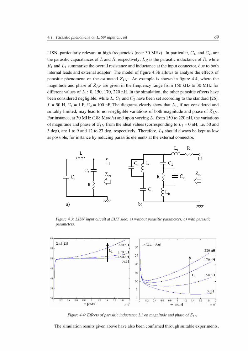
4.1. Parasitic phenomena on LISN input circuit 69
LISN, particularly relevant at high frequencies (near 30 MHz). In particular, CL and CR arethe parasitic capacitances of L and R, respectively; LR is the parasitic inductance of R, whileR1 and L1 summarize the overall resistance and inductance at the input connector, due to bothinternal leads and external adapter. The model of figure 4.3b allows to analyse the effects ofparasitic phenomena on the estimated ZIN . An example is shown in figure 4.4, where themagnitude and phase of ZIN are given in the frequency range from 150 kHz to 30 MHz fordifferent values of L1: 0, 150, 170, 220 nH. In the simulation, the other parasitic effects havebeen considered negligible, while L, C1 and C2 have been set according to the standard [26]:L = 50 H, C1 = 1 F, C2 = 100 nF. The diagrams clearly show that L1, if not considered andsuitably limited, may lead to non-negligible variations of both magnitude and phase of ZIN .For instance, at 30 MHz (188 Mrad/s) and upon varying L1 from 150 to 220 nH, the variationsof magnitude and phase of ZIN from the ideal values (corresponding to L1 = 0 nH, i.e. 50 and3 deg), are 1 to 9 and 12 to 27 deg, respectively. Therefore, L1 should always be kept as lowas possible, for instance by reducing parasitic elements at the external connector.
Figure 4.3: LISN input circuit at EUT side: a) without parasitic parameters, b) with parasiticparameters.
Figure 4.4: Effects of parasitic inductance L1 on magnitude and phase of ZIN .
The simulation results given above have also been confirmed through suitable experiments,
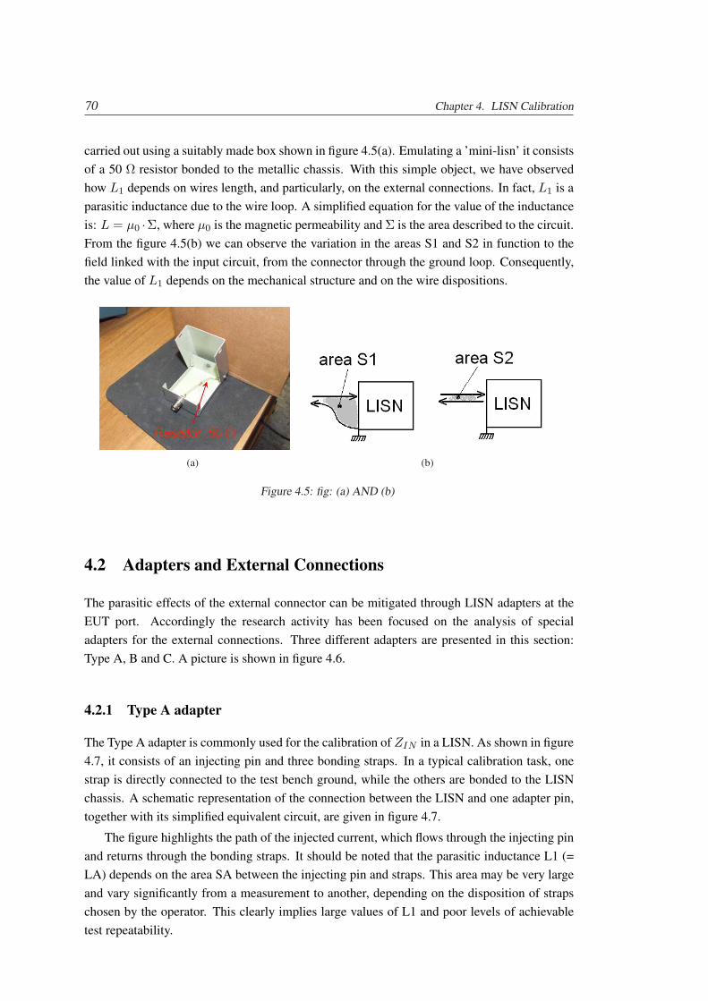
70 Chapter 4. LISN Calibration
carried out using a suitably made box shown in figure 4.5(a). Emulating a ’mini-lisn’ it consistsof a 50 Ω resistor bonded to the metallic chassis. With this simple object, we have observedhow L1 depends on wires length, and particularly, on the external connections. In fact, L1 is aparasitic inductance due to the wire loop. A simplified equation for the value of the inductanceis: L = µ0 ·Σ, where µ0 is the magnetic permeability and Σ is the area described to the circuit.From the figure 4.5(b) we can observe the variation in the areas S1 and S2 in function to thefield linked with the input circuit, from the connector through the ground loop. Consequently,the value of L1 depends on the mechanical structure and on the wire dispositions.
(a) (b)
Figure 4.5: fig: (a) AND (b)
4.2 Adapters and External Connections
The parasitic effects of the external connector can be mitigated through LISN adapters at theEUT port. Accordingly the research activity has been focused on the analysis of specialadapters for the external connections. Three different adapters are presented in this section:Type A, B and C. A picture is shown in figure 4.6.
4.2.1 Type A adapter
The Type A adapter is commonly used for the calibration of ZIN in a LISN. As shown in figure4.7, it consists of an injecting pin and three bonding straps. In a typical calibration task, onestrap is directly connected to the test bench ground, while the others are bonded to the LISNchassis. A schematic representation of the connection between the LISN and one adapter pin,together with its simplified equivalent circuit, are given in figure 4.7.
The figure highlights the path of the injected current, which flows through the injecting pinand returns through the bonding straps. It should be noted that the parasitic inductance L1 (=LA) depends on the area SA between the injecting pin and straps. This area may be very largeand vary significantly from a measurement to another, depending on the disposition of strapschosen by the operator. This clearly implies large values of L1 and poor levels of achievabletest repeatability.
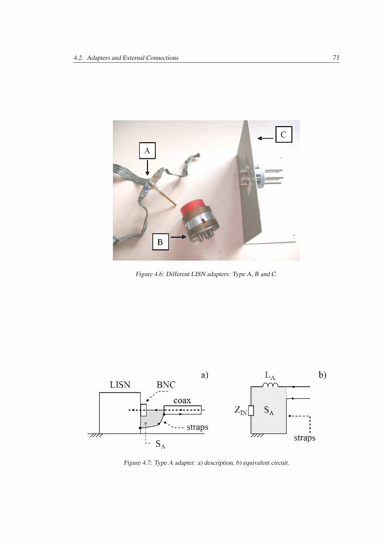
4.2. Adapters and External Connections 71
Figure 4.6: Different LISN adapters: Type A, B and C.
Figure 4.7: Type A adapter: a) description, b) equivalent circuit.
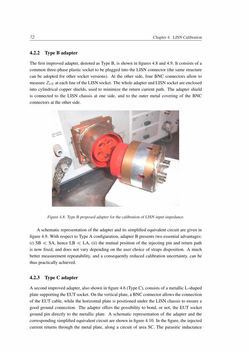
72 Chapter 4. LISN Calibration
4.2.2 Type B adapter
The first improved adapter, denoted as Type B, is shown in figures 4.8 and 4.9. It consists of acommon three-phase plastic socket to be plugged into the LISN connector (the same structurecan be adopted for other socket versions). At the other side, four BNC connectors allow tomeasure ZIN at each line of the LISN socket. The whole adapter and LISN socket are enclosedinto cylindrical copper shields, used to minimize the return current path. The adapter shieldis connected to the LISN chassis at one side, and to the outer metal covering of the BNCconnectors at the other side.
Figure 4.8: Type B proposed adapter for the calibration of LISN input impedance.
A schematic representation of the adapter and its simplified equivalent circuit are given infigure 4.9. With respect to Type A configuration, adapter B presents two essential advantages:(i) SB ¿ SA, hence LB ¿ LA, (ii) the mutual position of the injecting pin and return pathis now fixed, and does not vary depending on the user choice of straps disposition. A muchbetter measurement repeatability, and a consequently reduced calibration uncertainty, can bethus practically achieved.
4.2.3 Type C adapter
A second improved adapter, also shown in figure 4.6 (Type C), consists of a metallic L-shapedplate supporting the EUT socket. On the vertical plate, a BNC connector allows the connectionof the EUT cable, while the horizontal plate is positioned under the LISN chassis to ensure agood ground connection. The adapter offers the possibility to bond, or not, the EUT socketground pin directly to the metallic plate. A schematic representation of the adapter and thecorresponding simplified equivalent circuit are shown in figure 4.10. In the figure, the injectedcurrent returns through the metal plate, along a circuit of area SC. The parasitic inductance
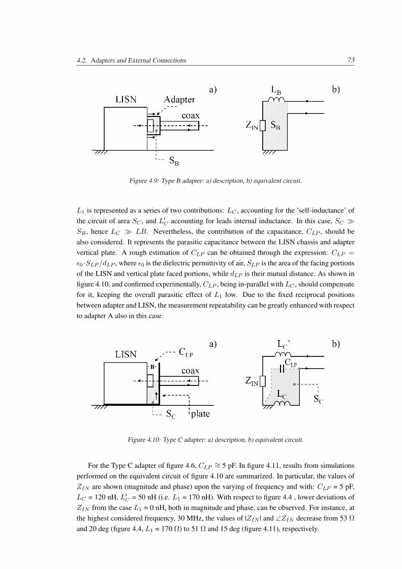
4.2. Adapters and External Connections 73
Figure 4.9: Type B adapter: a) description, b) equivalent circuit.
L1 is represented as a series of two contributions: LC , accounting for the ’self-inductance’ ofthe circuit of area SC , and L′C accounting for leads internal inductance. In this case, SC ÀSB , hence LC À LB. Nevertheless, the contribution of the capacitance, CLP , should bealso considered. It represents the parasitic capacitance between the LISN chassis and adaptervertical plate. A rough estimation of CLP can be obtained through the expression: CLP =ε0 ·SLP /dLP , where ε0 is the dielectric permittivity of air, SLP is the area of the facing portionsof the LISN and vertical plate faced portions, while dLP is their mutual distance. As shown infigure 4.10, and confirmed experimentally, CLP , being in-parallel with LC , should compensatefor it, keeping the overall parasitic effect of L1 low. Due to the fixed reciprocal positionsbetween adapter and LISN, the measurement repeatability can be greatly enhanced with respectto adapter A also in this case.
Figure 4.10: Type C adapter: a) description, b) equivalent circuit.
For the Type C adapter of figure 4.6, CLP∼= 5 pF. In figure 4.11, results from simulations
performed on the equivalent circuit of figure 4.10 are summarized. In particular, the values ofZIN are shown (magnitude and phase) upon the varying of frequency and with: CLP = 5 pF,LC = 120 nH, L′C = 50 nH (i.e. L1 = 170 nH). With respect to figure 4.4 , lower deviations ofZIN from the case L1 = 0 nH, both in magnitude and phase, can be observed. For instance, atthe highest considered frequency, 30 MHz, the values of |ZIN | and ∠ZIN decrease from 53 Ωand 20 deg (figure 4.4, L1 = 170 Ω) to 51 Ω and 15 deg (figure 4.11), respectively.
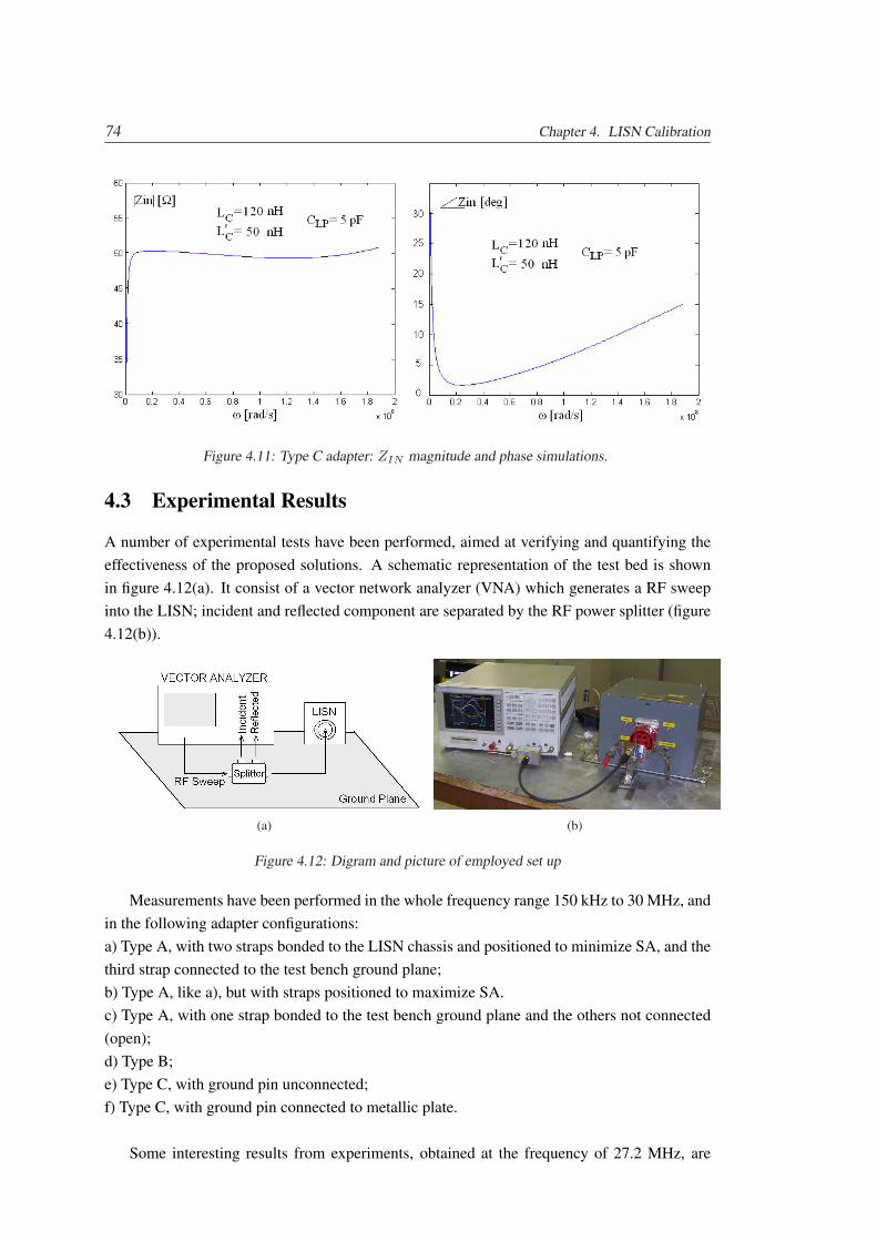
74 Chapter 4. LISN Calibration
Figure 4.11: Type C adapter: ZIN magnitude and phase simulations.
4.3 Experimental Results
A number of experimental tests have been performed, aimed at verifying and quantifying theeffectiveness of the proposed solutions. A schematic representation of the test bed is shownin figure 4.12(a). It consist of a vector network analyzer (VNA) which generates a RF sweepinto the LISN; incident and reflected component are separated by the RF power splitter (figure4.12(b)).
(a) (b)
Figure 4.12: Digram and picture of employed set up
Measurements have been performed in the whole frequency range 150 kHz to 30 MHz, andin the following adapter configurations:a) Type A, with two straps bonded to the LISN chassis and positioned to minimize SA, and thethird strap connected to the test bench ground plane;b) Type A, like a), but with straps positioned to maximize SA.c) Type A, with one strap bonded to the test bench ground plane and the others not connected(open);d) Type B;e) Type C, with ground pin unconnected;f) Type C, with ground pin connected to metallic plate.
Some interesting results from experiments, obtained at the frequency of 27.2 MHz, are
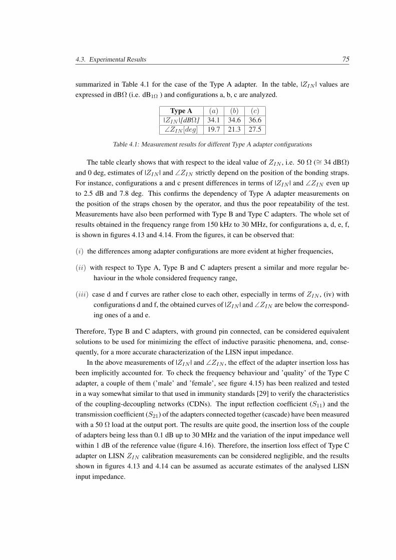
4.3. Experimental Results 75
summarized in Table 4.1 for the case of the Type A adapter. In the table, |ZIN | values areexpressed in dBΩ (i.e. dB1Ω ) and configurations a, b, c are analyzed.
Type A (a) (b) (c)|ZIN |[dBΩ] 34.1 34.6 36.6∠ZIN [deg] 19.7 21.3 27.5
Table 4.1: Measurement results for different Type A adapter configurations
The table clearly shows that with respect to the ideal value of ZIN , i.e. 50 Ω (∼= 34 dBΩ)and 0 deg, estimates of |ZIN | and ∠ZIN strictly depend on the position of the bonding straps.For instance, configurations a and c present differences in terms of |ZIN | and ∠ZIN even upto 2.5 dB and 7.8 deg. This confirms the dependency of Type A adapter measurements onthe position of the straps chosen by the operator, and thus the poor repeatability of the test.Measurements have also been performed with Type B and Type C adapters. The whole set ofresults obtained in the frequency range from 150 kHz to 30 MHz, for configurations a, d, e, f,is shown in figures 4.13 and 4.14. From the figures, it can be observed that:
(i) the differences among adapter configurations are more evident at higher frequencies,
(ii) with respect to Type A, Type B and C adapters present a similar and more regular be-haviour in the whole considered frequency range,
(iii) case d and f curves are rather close to each other, especially in terms of ZIN , (iv) withconfigurations d and f, the obtained curves of |ZIN | and ∠ZIN are below the correspond-ing ones of a and e.
Therefore, Type B and C adapters, with ground pin connected, can be considered equivalentsolutions to be used for minimizing the effect of inductive parasitic phenomena, and, conse-quently, for a more accurate characterization of the LISN input impedance.
In the above measurements of |ZIN | and ∠ZIN , the effect of the adapter insertion loss hasbeen implicitly accounted for. To check the frequency behaviour and ’quality’ of the Type Cadapter, a couple of them (’male’ and ’female’, see figure 4.15) has been realized and testedin a way somewhat similar to that used in immunity standards [29] to verify the characteristicsof the coupling-decoupling networks (CDNs). The input reflection coefficient (S11) and thetransmission coefficient (S21) of the adapters connected together (cascade) have been measuredwith a 50 Ω load at the output port. The results are quite good, the insertion loss of the coupleof adapters being less than 0.1 dB up to 30 MHz and the variation of the input impedance wellwithin 1 dB of the reference value (figure 4.16). Therefore, the insertion loss effect of Type Cadapter on LISN ZIN calibration measurements can be considered negligible, and the resultsshown in figures 4.13 and 4.14 can be assumed as accurate estimates of the analysed LISNinput impedance.
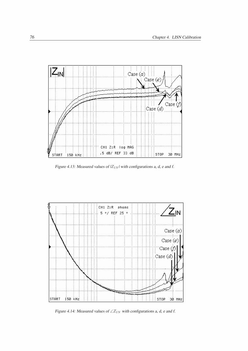
76 Chapter 4. LISN Calibration
Figure 4.13: Measured values of |ZIN | with configurations a, d, e and f.
Figure 4.14: Measured values of ∠ZIN with configurations a, d, e and f.
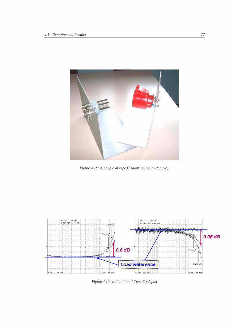
4.3. Experimental Results 77
Figure 4.15: A couple of type C adapters (male - female).
Figure 4.16: calibration of Type C adapter


Chapter 5
Uncertainty Evaluation in ESD Tests
When two non-conductive materials are rubbed together or separated, electrons from one ma-terial are transferred to the other. This results in the accumulation of triboelectric charge onthe surface of the material. The amount of charge caused by movement of the materials is afunction of the separation of the materials in the triboelectric series. Additional factors are thecloseness of contact, rate of separation and humidity [24]. The human body can be charged bytriboelectric induction to several kilovolt.When the body approaches a conductive object, the charge is transferred to that object nor-mally via a spark, when the potential gradient across the narrowing air gap is high enoughto cause breakdown. Electrostatic discharges (ESDs) represent a well-known phenomenon inelectronics The effects of such phenomena can be rather critical for electronic devices, and mayprovoke system failures or even permanent damages. In order to assess the immunity level ofan equipment under test (EUT) to ESD, specific standards can be followed [30], [31]. In thesestandards, the immunity requirements and the test methods are defined for both contact and airdischarge. The characteristics of the ESD discharges are also provided. Standard prescriptionsare used in the setup stage of the ESD generator (also known as "gun") in order to providedischarges similar to those generated by the human body.One important issue of ESD tests is the evaluation of the test uncertainty, and in particularthe uncertainty contribution associated to repeatability. In these tests, in fact, repeatability isusually very low and the corresponding uncertainty contribution is typically rather high. Inthe literature, the repeatability of ESD tests is investigated in-depth in a number of specificcontributions. For instance, [32] provides interesting results from an international comparisonamong ESD-generator calibration tasks. The results reported in this paper confirm the highvariability of ESD test outputs and underline the importance of the measurement setup, which,in the comparison, was different from one laboratory to another. In [33], the uncertainty bud-get of an ESD test is discussed, with special regard to some specific uncertainty factors likemeasurement repeatability, cable and adaptor loss and time resolution. The uncertainty contri-butions in an ESD test are also dealt with in [30]. This standard suggests the diagram shownin figure 5.1 to take into account the influence on the test of parameters like the position andorientation of the ESD gun.
Unfortunately, in most such contributions attention is paid to the only case of contact dis-
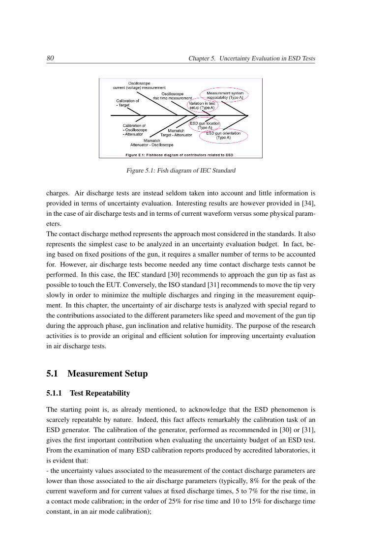
80 Chapter 5. Uncertainty Evaluation in ESD Tests
Figure 5.1: Fish diagram of IEC Standard
charges. Air discharge tests are instead seldom taken into account and little information isprovided in terms of uncertainty evaluation. Interesting results are however provided in [34],in the case of air discharge tests and in terms of current waveform versus some physical param-eters.The contact discharge method represents the approach most considered in the standards. It alsorepresents the simplest case to be analyzed in an uncertainty evaluation budget. In fact, be-ing based on fixed positions of the gun, it requires a smaller number of terms to be accountedfor. However, air discharge tests become needed any time contact discharge tests cannot beperformed. In this case, the IEC standard [30] recommends to approach the gun tip as fast aspossible to touch the EUT. Conversely, the ISO standard [31] recommends to move the tip veryslowly in order to minimize the multiple discharges and ringing in the measurement equip-ment. In this chapter, the uncertainty of air discharge tests is analyzed with special regard tothe contributions associated to the different parameters like speed and movement of the gun tipduring the approach phase, gun inclination and relative humidity. The purpose of the researchactivities is to provide an original and efficient solution for improving uncertainty evaluationin air discharge tests.
5.1 Measurement Setup
5.1.1 Test Repeatability
The starting point is, as already mentioned, to acknowledge that the ESD phenomenon isscarcely repeatable by nature. Indeed, this fact affects remarkably the calibration task of anESD generator. The calibration of the generator, performed as recommended in [30] or [31],gives the first important contribution when evaluating the uncertainty budget of an ESD test.From the examination of many ESD calibration reports produced by accredited laboratories, itis evident that:- the uncertainty values associated to the measurement of the contact discharge parameters arelower than those associated to the air discharge parameters (typically, 8% for the peak of thecurrent waveform and for current values at fixed discharge times, 5 to 7% for the rise time, ina contact mode calibration; in the order of 25% for rise time and 10 to 15% for discharge timeconstant, in an air mode calibration);
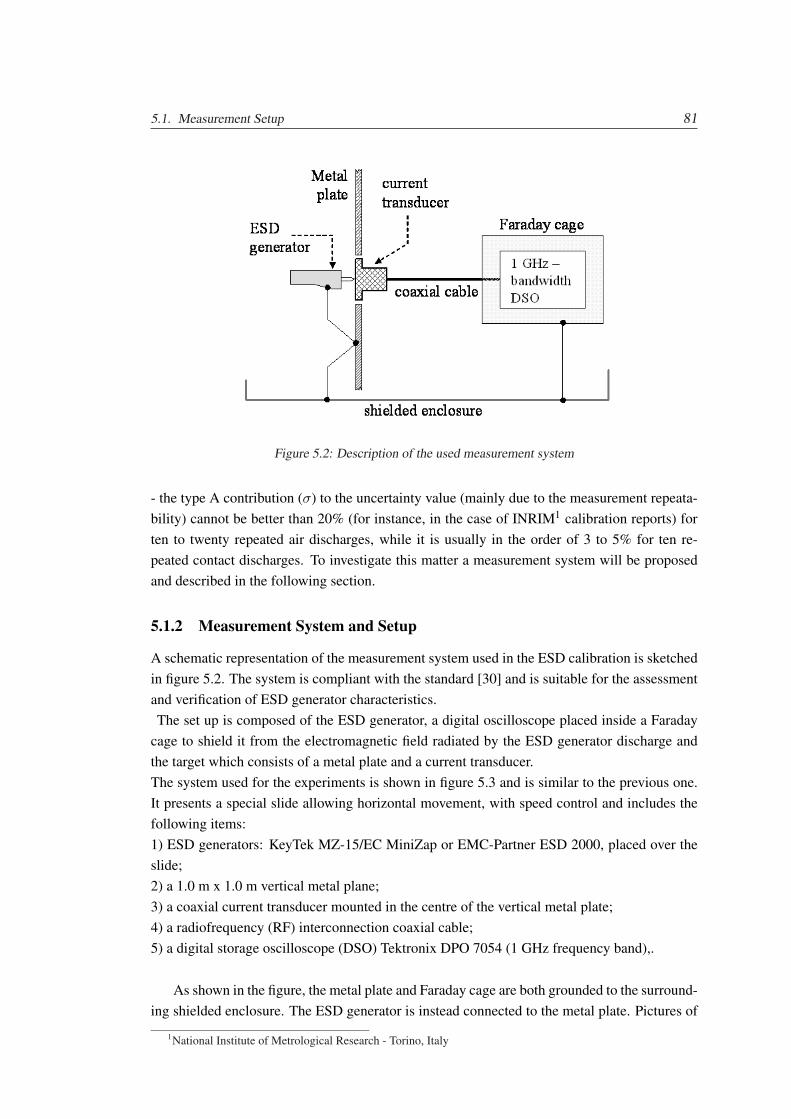
5.1. Measurement Setup 81
Figure 5.2: Description of the used measurement system
- the type A contribution (σ) to the uncertainty value (mainly due to the measurement repeata-bility) cannot be better than 20% (for instance, in the case of INRIM1 calibration reports) forten to twenty repeated air discharges, while it is usually in the order of 3 to 5% for ten re-peated contact discharges. To investigate this matter a measurement system will be proposedand described in the following section.
5.1.2 Measurement System and Setup
A schematic representation of the measurement system used in the ESD calibration is sketchedin figure 5.2. The system is compliant with the standard [30] and is suitable for the assessmentand verification of ESD generator characteristics.The set up is composed of the ESD generator, a digital oscilloscope placed inside a Faraday
cage to shield it from the electromagnetic field radiated by the ESD generator discharge andthe target which consists of a metal plate and a current transducer.The system used for the experiments is shown in figure 5.3 and is similar to the previous one.It presents a special slide allowing horizontal movement, with speed control and includes thefollowing items:1) ESD generators: KeyTek MZ-15/EC MiniZap or EMC-Partner ESD 2000, placed over theslide;2) a 1.0 m x 1.0 m vertical metal plane;3) a coaxial current transducer mounted in the centre of the vertical metal plate;4) a radiofrequency (RF) interconnection coaxial cable;5) a digital storage oscilloscope (DSO) Tektronix DPO 7054 (1 GHz frequency band),.
As shown in the figure, the metal plate and Faraday cage are both grounded to the surround-ing shielded enclosure. The ESD generator is instead connected to the metal plate. Pictures of
1National Institute of Metrological Research - Torino, Italy
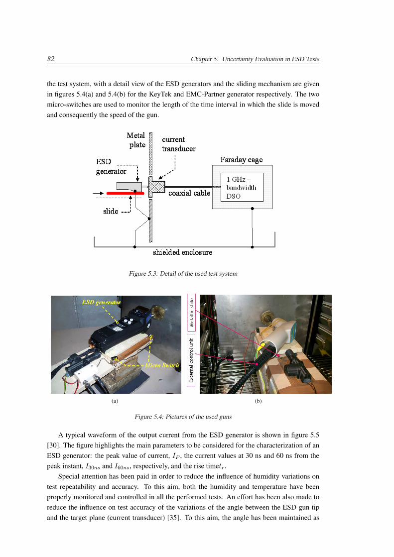
82 Chapter 5. Uncertainty Evaluation in ESD Tests
the test system, with a detail view of the ESD generators and the sliding mechanism are givenin figures 5.4(a) and 5.4(b) for the KeyTek and EMC-Partner generator respectively. The twomicro-switches are used to monitor the length of the time interval in which the slide is movedand consequently the speed of the gun.
Figure 5.3: Detail of the used test system
(a) (b)
Figure 5.4: Pictures of the used guns
A typical waveform of the output current from the ESD generator is shown in figure 5.5[30]. The figure highlights the main parameters to be considered for the characterization of anESD generator: the peak value of current, IP , the current values at 30 ns and 60 ns from thepeak instant, I30ns and I60ns, respectively, and the rise timetr.
Special attention has been paid in order to reduce the influence of humidity variations ontest repeatability and accuracy. To this aim, both the humidity and temperature have beenproperly monitored and controlled in all the performed tests. An effort has been also made toreduce the influence on test accuracy of the variations of the angle between the ESD gun tipand the target plane (current transducer) [35]. To this aim, the angle has been maintained as
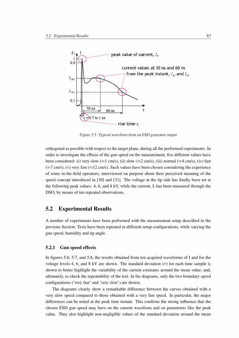
5.2. Experimental Results 83
Figure 5.5: Typical waveform from an ESD generator output
orthogonal as possible with respect to the target plane, during all the performed experiments. Inorder to investigate the effects of the gun speed on the measurement, five different values havebeen considered: (i) very slow (≈1 cm/s), (ii) slow (≈2 cm/s), (iii) normal (≈4 cm/s), (iv) fast(≈7 cm/s), (v) very fast (≈12 cm/s). Such values have been chosen considering the experienceof some in-the-field operators, interviewed on purpose about their perceived meaning of thespeed concept introduced in [30] and [31]. The voltage at the tip side has finally been set atthe following peak values: 4, 6, and 8 kV, while the current, I, has been measured through theDSO, by means of ten repeated observations.
5.2 Experimental Results
A number of experiments have been performed with the measurement setup described in theprevious Section. Tests have been repeated in different setup configurations, while varying thegun speed, humidity and tip angle.
5.2.1 Gun speed effects
In figures 5.6, 5.7, and 5.8, the results obtained from ten acquired waveforms of I and for thevoltage levels 4, 6, and 8 kV are shown. The standard deviation (σ) for each time sample isshown to better highlight the variability of the current estimates around the mean value, and,ultimately, to check the repeatability of the test. In the diagrams, only the two boundary speedconfigurations (’very fast’ and ’very slow’) are shown.
The diagrams clearly show a remarkable difference between the curves obtained with avery slow speed compared to those obtained with a very fast speed. In particular, the majordifferences can be noted at the peak time instant. This confirms the strong influence that thechosen ESD gun speed may have on the current waveform and on parameters like the peakvalue. They also highlight non-negligible values of the standard deviation around the mean
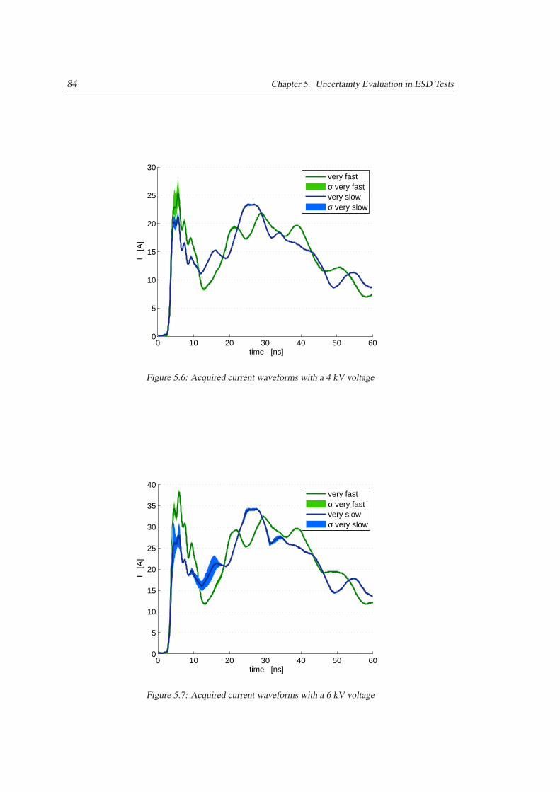
84 Chapter 5. Uncertainty Evaluation in ESD Tests
0 10 20 30 40 50 600
5
10
15
20
25
30
time [ns]
I [
A]
very fastσ very fastvery slowσ very slow
Figure 5.6: Acquired current waveforms with a 4 kV voltage
0 10 20 30 40 50 600
5
10
15
20
25
30
35
40
time [ns]
I [
A]
very fastσ very fastvery slowσ very slow
Figure 5.7: Acquired current waveforms with a 6 kV voltage
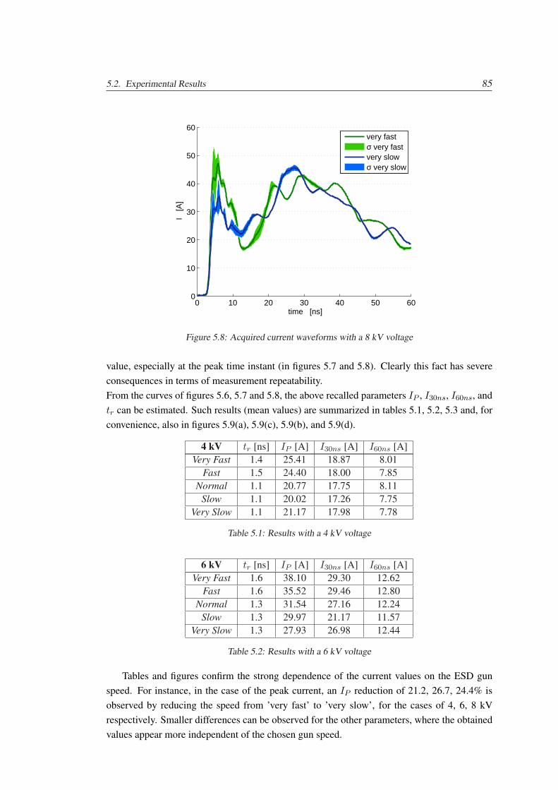
5.2. Experimental Results 85
0 10 20 30 40 50 600
10
20
30
40
50
60
time [ns]
I [
A]
very fastσ very fastvery slowσ very slow
Figure 5.8: Acquired current waveforms with a 8 kV voltage
value, especially at the peak time instant (in figures 5.7 and 5.8). Clearly this fact has severeconsequences in terms of measurement repeatability.From the curves of figures 5.6, 5.7 and 5.8, the above recalled parameters IP , I30ns, I60ns, andtr can be estimated. Such results (mean values) are summarized in tables 5.1, 5.2, 5.3 and, forconvenience, also in figures 5.9(a), 5.9(c), 5.9(b), and 5.9(d).
4 kV tr [ns] IP [A] I30ns [A] I60ns [A]Very Fast 1.4 25.41 18.87 8.01
Fast 1.5 24.40 18.00 7.85Normal 1.1 20.77 17.75 8.11
Slow 1.1 20.02 17.26 7.75Very Slow 1.1 21.17 17.98 7.78
Table 5.1: Results with a 4 kV voltage
6 kV tr [ns] IP [A] I30ns [A] I60ns [A]Very Fast 1.6 38.10 29.30 12.62
Fast 1.6 35.52 29.46 12.80Normal 1.3 31.54 27.16 12.24
Slow 1.3 29.97 21.17 11.57Very Slow 1.3 27.93 26.98 12.44
Table 5.2: Results with a 6 kV voltage
Tables and figures confirm the strong dependence of the current values on the ESD gunspeed. For instance, in the case of the peak current, an IP reduction of 21.2, 26.7, 24.4% isobserved by reducing the speed from ’very fast’ to ’very slow’, for the cases of 4, 6, 8 kVrespectively. Smaller differences can be observed for the other parameters, where the obtainedvalues appear more independent of the chosen gun speed.
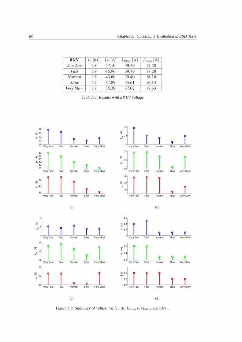
86 Chapter 5. Uncertainty Evaluation in ESD Tests
8 kV tr [ns] IP [A] I30ns [A] I60ns [A]Very Fast 1.8 47.10 39.59 17.28
Fast 1.8 46.96 39.76 17.28Normal 1.8 43.60 39.40 16.16
Slow 1.7 37.89 35.61 16.15Very Slow 1.7 35.39 37.02 17.33
Table 5.3: Results with a 8 kV voltage
Very Fast Fast Normal Slow Very Slow18
20
22
24
26
Ip
[A]
Very Fast Fast Normal Slow Very Slow283032343638
Ip
[A]
Very Fast Fast Normal Slow Very Slow35
40
45
Ip
[A]
(a)
Very Fast Fast Normal Slow Very Slow17
18
19
I 30
[A]
Very Fast Fast Normal Slow Very Slow20
25
30
I 30
[A]
Very Fast Fast Normal Slow Very Slow
36
38
40
I 30
[A]
(b)
Very Fast Fast Normal Slow Very Slow7
8
9
I 60
[A]
Very Fast Fast Normal Slow Very Slow11
12
13
I 60
[A]
Very Fast Fast Normal Slow Very Slow16
17
18
I 60
[A]
(c)
Very Fast Fast Normal Slow Very Slow1
1.2
1.4
1.6
tr
[ns]
Very Fast Fast Normal Slow Very Slow1.2
1.4
1.6
tr
[ns]
Very Fast Fast Normal Slow Very Slow1.6
1.7
1.8
tr
[ns]
(d)
Figure 5.9: Summary of values: (a) IP , (b) I30ns, (c) I60ns and (d) tr,
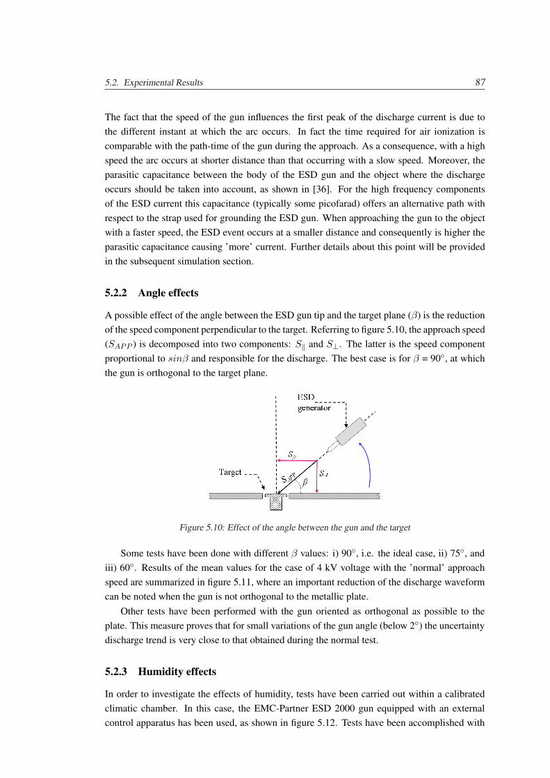
5.2. Experimental Results 87
The fact that the speed of the gun influences the first peak of the discharge current is due tothe different instant at which the arc occurs. In fact the time required for air ionization iscomparable with the path-time of the gun during the approach. As a consequence, with a highspeed the arc occurs at shorter distance than that occurring with a slow speed. Moreover, theparasitic capacitance between the body of the ESD gun and the object where the dischargeoccurs should be taken into account, as shown in [36]. For the high frequency componentsof the ESD current this capacitance (typically some picofarad) offers an alternative path withrespect to the strap used for grounding the ESD gun. When approaching the gun to the objectwith a faster speed, the ESD event occurs at a smaller distance and consequently is higher theparasitic capacitance causing ’more’ current. Further details about this point will be providedin the subsequent simulation section.
5.2.2 Angle effects
A possible effect of the angle between the ESD gun tip and the target plane (β) is the reductionof the speed component perpendicular to the target. Referring to figure 5.10, the approach speed(SAPP ) is decomposed into two components: S‖ and S⊥. The latter is the speed componentproportional to sinβ and responsible for the discharge. The best case is for β = 90, at whichthe gun is orthogonal to the target plane.
Figure 5.10: Effect of the angle between the gun and the target
Some tests have been done with different β values: i) 90, i.e. the ideal case, ii) 75, andiii) 60. Results of the mean values for the case of 4 kV voltage with the ’normal’ approachspeed are summarized in figure 5.11, where an important reduction of the discharge waveformcan be noted when the gun is not orthogonal to the metallic plate.
Other tests have been performed with the gun oriented as orthogonal as possible to theplate. This measure proves that for small variations of the gun angle (below 2) the uncertaintydischarge trend is very close to that obtained during the normal test.
5.2.3 Humidity effects
In order to investigate the effects of humidity, tests have been carried out within a calibratedclimatic chamber. In this case, the EMC-Partner ESD 2000 gun equipped with an externalcontrol apparatus has been used, as shown in figure 5.12. Tests have been accomplished with
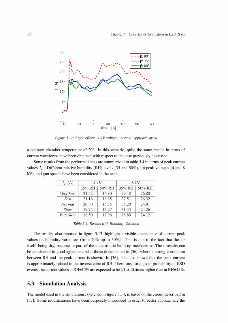
88 Chapter 5. Uncertainty Evaluation in ESD Tests
0 10 20 30 40 50 60−5
0
5
10
15
20
25
30
time [ns]
I [
A]
β: 90°β: 75°β: 60°
Figure 5.11: Angle effects: 4 kV voltage, ’normal’ approach speed
a constant chamber temperature of 20. In this scenario, quite the same results in terms ofcurrent waveforms have been obtained with respect to the case previously discussed.
Some results from the performed tests are summarized in table 5.4 in terms of peak currentvalues IP . Different relative humidity (RH) levels (35 and 50%), tip peak voltages (4 and 8kV), and gun speeds have been considered in the tests.
IP [A] 4 kV 8 kV35% RH 50% RH 35% RH 50% RH
Very Fast 21.52 16.80 39.48 26.80Fast 21.16 16.35 37.51 26.32
Normal 20.80 15.75 35.20 24.91Slow 19.75 15.27 31.33 24.26
Very Slow 18.50 12.96 28.85 24.12
Table 5.4: Results with Humidity Variation
The results, also reported in figure 5.13, highlight a visible dependence of current peakvalues on humidity variations (from 20% up to 30%). This is due to the fact that the airitself, being dry, becomes a part of the electrostatic build-up mechanism. These results canbe considered in good agreement with those documented in [36], where a strong correlationbetween RH and the peak current is shown. In [36], it is also shown that the peak currentis approximately related to the inverse cube of RH. Therefore, for a given probability of ESDevents, the current values at RH=15% are expected to be 20 to 40 times higher than at RH=45%.
5.3 Simulation Analysis
The model used in the simulations, sketched in figure 5.14, is based on the circuit described in[37]. Some modifications have been purposely introduced in order to better approximate the
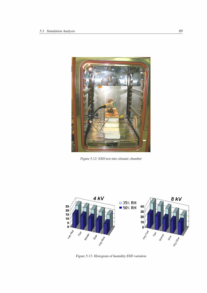
5.3. Simulation Analysis 89
Figure 5.12: ESD test into climatic chamber
Figure 5.13: Histogram of humidity ESD variation
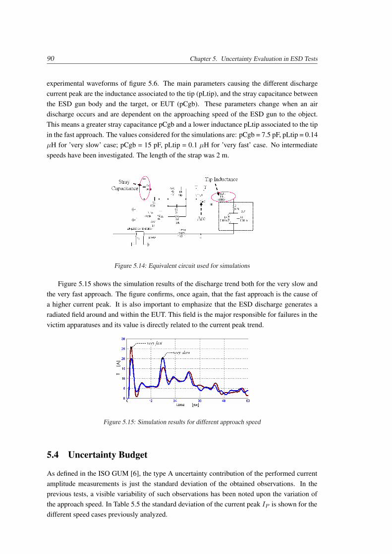
90 Chapter 5. Uncertainty Evaluation in ESD Tests
experimental waveforms of figure 5.6. The main parameters causing the different dischargecurrent peak are the inductance associated to the tip (pLtip), and the stray capacitance betweenthe ESD gun body and the target, or EUT (pCgb). These parameters change when an airdischarge occurs and are dependent on the approaching speed of the ESD gun to the object.This means a greater stray capacitance pCgb and a lower inductance pLtip associated to the tipin the fast approach. The values considered for the simulations are: pCgb = 7.5 pF, pLtip = 0.14µH for ’very slow’ case; pCgb = 15 pF, pLtip = 0.1 µH for ’very fast’ case. No intermediatespeeds have been investigated. The length of the strap was 2 m.
Figure 5.14: Equivalent circuit used for simulations
Figure 5.15 shows the simulation results of the discharge trend both for the very slow andthe very fast approach. The figure confirms, once again, that the fast approach is the cause ofa higher current peak. It is also important to emphasize that the ESD discharge generates aradiated field around and within the EUT. This field is the major responsible for failures in thevictim apparatuses and its value is directly related to the current peak trend.
Figure 5.15: Simulation results for different approach speed
5.4 Uncertainty Budget
As defined in the ISO GUM [6], the type A uncertainty contribution of the performed currentamplitude measurements is just the standard deviation of the obtained observations. In theprevious tests, a visible variability of such observations has been noted upon the variation ofthe approach speed. In Table 5.5 the standard deviation of the current peak IP is shown for thedifferent speed cases previously analyzed.
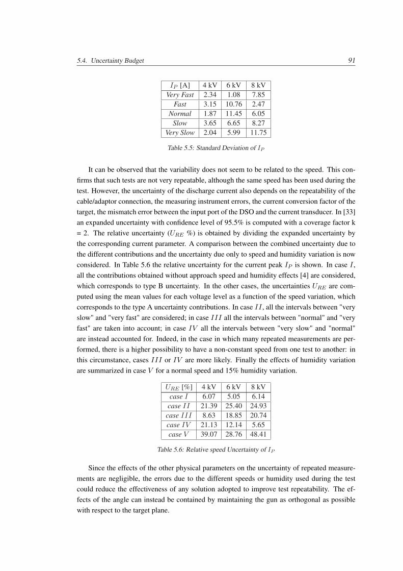
5.4. Uncertainty Budget 91
IP [A] 4 kV 6 kV 8 kVVery Fast 2.34 1.08 7.85
Fast 3.15 10.76 2.47Normal 1.87 11.45 6.05
Slow 3.65 6.65 8.27Very Slow 2.04 5.99 11.75
Table 5.5: Standard Deviation of IP
It can be observed that the variability does not seem to be related to the speed. This con-firms that such tests are not very repeatable, although the same speed has been used during thetest. However, the uncertainty of the discharge current also depends on the repeatability of thecable/adaptor connection, the measuring instrument errors, the current conversion factor of thetarget, the mismatch error between the input port of the DSO and the current transducer. In [33]an expanded uncertainty with confidence level of 95.5% is computed with a coverage factor k= 2. The relative uncertainty (URE %) is obtained by dividing the expanded uncertainty bythe corresponding current parameter. A comparison between the combined uncertainty due tothe different contributions and the uncertainty due only to speed and humidity variation is nowconsidered. In Table 5.6 the relative uncertainty for the current peak IP is shown. In case I ,all the contributions obtained without approach speed and humidity effects [4] are considered,which corresponds to type B uncertainty. In the other cases, the uncertainties URE are com-puted using the mean values for each voltage level as a function of the speed variation, whichcorresponds to the type A uncertainty contributions. In case II , all the intervals between "veryslow" and "very fast" are considered; in case III all the intervals between "normal" and "veryfast" are taken into account; in case IV all the intervals between "very slow" and "normal"are instead accounted for. Indeed, in the case in which many repeated measurements are per-formed, there is a higher possibility to have a non-constant speed from one test to another: inthis circumstance, cases III or IV are more likely. Finally the effects of humidity variationare summarized in case V for a normal speed and 15% humidity variation.
URE [%] 4 kV 6 kV 8 kVcase I 6.07 5.05 6.14
case II 21.39 25.40 24.93case III 8.63 18.85 20.74case IV 21.13 12.14 5.65case V 39.07 28.76 48.41
Table 5.6: Relative speed Uncertainty of IP
Since the effects of the other physical parameters on the uncertainty of repeated measure-ments are negligible, the errors due to the different speeds or humidity used during the testcould reduce the effectiveness of any solution adopted to improve test repeatability. The ef-fects of the angle can instead be contained by maintaining the gun as orthogonal as possiblewith respect to the target plane.

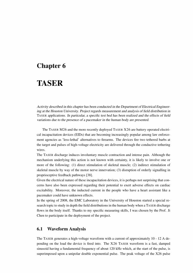
Chapter 6
TASER
Activity described in this chapter has been conducted in the Department of Electrical Engineer-ing at the Houston University. Project regards measurement and analysis of field distribution inTASER applications. In particular, a specific test bed has been realized and the effects of fieldvariations due to the presence of a pacemaker in the human body are presented.
The TASER M26 and the more recently deployed TASER X26 are battery operated electri-cal incapacitation devices (EIDs) that are becoming increasingly popular among law enforce-ment agencies as ’less-lethal’ alternatives to firearms. The devices fire two tethered barbs atthe target and pulses of high-voltage electricity are delivered through the conductive tetheringwires.The TASER discharge induces involuntary muscle contraction and intense pain. Although themechanism underlying this action is not known with certainty, it is likely to involve one ormore of the following: (1) direct stimulation of skeletal muscle; (2) indirect stimulation ofskeletal muscle by way of the motor nerve innervation; (3) disruption of orderly signalling inproprioceptive feedback pathways [38].Given the electrical nature of these incapacitation devices, it is perhaps not surprising that con-cerns have also been expressed regarding their potential to exert adverse effects on cardiacexcitability. Moreover, the inducted current in the people who have a heart assistant like apacemaker could have unknown effects.In the spring of 2008, the EMC Laboratory in the University of Houston started a special re-search topic to study in depth the field distributions in the human body when a TASER dischargeflows in the body itself. Thanks to my specific measuring skills, I was chosen by the Prof. JiChen to participate in the deployment of the project.
6.1 Waveform Analysis
The TASER generates a high-voltage waveform with a current of approximately 10 - 12 A de-pending on the load the device is fired into. The X26 TASER waveform is a fast, dampedsinusoid having a fundamental frequency of about 120 kHz which, at the start of the pulse, issuperimposed upon a unipolar double exponential pulse. The peak voltage of the X26 pulse
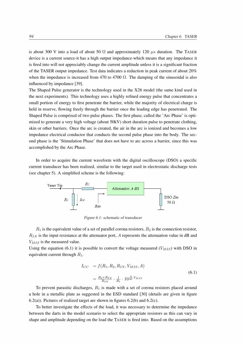
94 Chapter 6. TASER
is about 300 V into a load of about 50 Ω and approximately 120 µs duration. The TASER
device is a current source-it has a high output impedance-which means that any impedance itis fired into will not appreciably change the current amplitude unless it is a significant fractionof the TASER output impedance. Test data indicates a reduction in peak current of about 20%when the impedance is increased from 470 to 4700 Ω. The damping of the sinusoidal is alsoinfluenced by impedance [39].The Shaped Pulse generator is the technology used in the X26 model (the same kind used inthe next experiments). This technology uses a highly refined energy pulse that concentrates asmall portion of energy to first penetrate the barrier, while the majority of electrical charge isheld in reserve, flowing freely through the barrier once the leading edge has penetrated. TheShaped Pulse is comprised of two pulse phases. The first phase, called the ’Arc Phase’ is opti-mized to generate a very high voltage (about 50kV) short duration pulse to penetrate clothing,skin or other barriers. Once the arc is created, the air in the arc is ionized and becomes a lowimpedance electrical conductor that conducts the second pulse phase into the body. The sec-ond phase is the ’Stimulation Phase’ that does not have to arc across a barrier, since this wasaccomplished by the Arc Phase.
In order to acquire the current waveform with the digital oscilloscope (DSO) a specificcurrent transducer has been realized, similar to the target used in electrostatic discharge tests(see chapter 5). A simplified scheme is the following:
Figure 6.1: schematic of transducer
R1 is the equivalent value of a set of parallel corona resistors, R2 is the connection resistor,RIN is the input resistance at the attenuator port, A represents the attenuation value in dB andVMIS is the measured value.Using the equation (6.1) it is possible to convert the voltage measured (VMIS) with DSO inequivalent current through R1.
ICC = f(R1, R2, RIN , VMIS , A)
= R2+RINRIN
· 1R1· 10
A20·VMIS
(6.1)
To prevent parasitic discharges, R1 is made with a set of corona resistors placed arounda hole in a metallic plate as suggested in the ESD standard [30] (details are given in figure6.2(a)). Pictures of realized target are shown in figures 6.2(b) and 6.2(c).
To better investigate the effects of the load, it was necessary to determine the impedancebetween the darts in the model scenario to select the appropriate resistors as this can vary inshape and amplitude depending on the load the TASER is fired into. Based on the assumptions
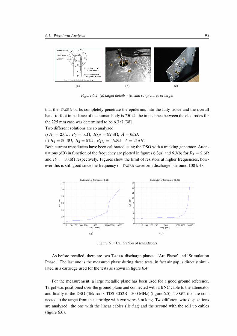
6.1. Waveform Analysis 95
(a) (b) (c)
Figure 6.2: (a) target details - (b) and (c) pictures of target
that the TASER barbs completely penetrate the epidermis into the fatty tissue and the overallhand-to-foot impedance of the human body is 750 Ω, the impedance between the electrodes forthe 225 mm case was determined to be 6.3 Ω [38].Two different solutions are so analyzed:i) R1 = 2.6Ω, R2 = 51Ω, RIN = 92.8Ω, A = 6dB;ii) R1 = 50.6Ω, R2 = 51Ω, RIN = 45.8Ω, A = 21dB.Both current transducers have been calibrated using the DSO with a tracking generator. Atten-uations (dB) in function of the frequency are plotted in figures 6.3(a) and 6.3(b) for R1 = 2.6Ωand R1 = 50.6Ω respectively. Figures show the limit of resistors at higher frequencies, how-ever this is still good since the frequency of TASER waveform discharge is around 100 kHz.
1 10 50 100 200 500 10005000 100005
10
15
20
25
30
35 Calibration of Transducer 2.6 Ω
freq [kHz]
Att
[dB
]
(a)
1 10 50 100 200 500 10005000 100005
6
7
8
9
10
11
12
13 Calibration of Transducer 50.6 Ω
freq [kHz]
Att
[dB
]
(b)
Figure 6.3: Calibration of transducers
As before recalled, there are two TASER discharge phases: ’Arc Phase’ and ’StimulationPhase’. The last one is the measured phase during these tests, in fact air gap is directly simu-lated in a cartridge used for the tests as shown in figure 6.4.
For the measurement, a large metallic plane has been used for a good ground reference.Target was positioned over the ground plane and connected with a BNC cable to the attenuatorand finally to the DSO (Tektronix TDS 3052B - 500 MHz) (figure 6.5). TASER tips are con-nected to the target from the cartridge with two wires 3 m long. Two different wire dispositionsare analyzed: the one with the linear cables (lie flat) and the second with the roll up cables(figure 6.6).
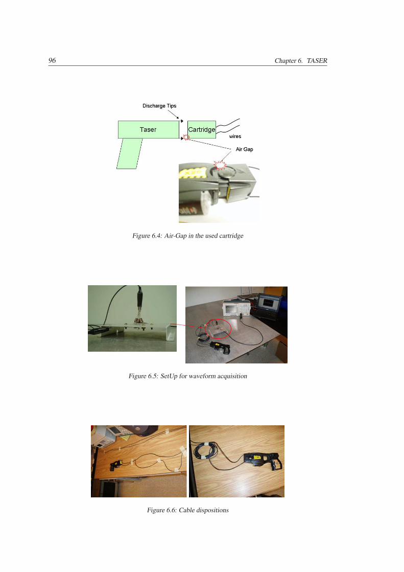
96 Chapter 6. TASER
Figure 6.4: Air-Gap in the used cartridge
Figure 6.5: SetUp for waveform acquisition
Figure 6.6: Cable dispositions
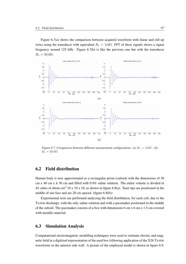
6.2. Field distribution 97
Figure 6.7(a) shows the comparison between acquired waveform with linear and roll upwires using the transducer with equivalent R1 = 2.6Ω. FFT of these signals shows a signalfrequency around 125 kHz. Figure 6.7(b) is like the previous one but with the transducerR1 = 50.6Ω.
−20 0 20 40 60 80 100 120 140 160 180 200−2
−1.5
−1
−0.5
0
0.5
1
1.5
2
Linear Cable with R1=2.6 Ω
time [µs]
I [
A]
−20 0 20 40 60 80 100 120 140 160 180 200−2
−1.5
−1
−0.5
0
0.5
1
1.5
2
RollUp Cable with R1=2.6 Ω
time [µs]
I [
A]
(a)
−20 0 20 40 60 80 100 120 140 160 180 200−2
−1.5
−1
−0.5
0
0.5
1
1.5
2
Linear Cable with R1=50.6 Ω
time [µs]
I [
A]
−20 0 20 40 60 80 100 120 140 160 180 200−2
−1.5
−1
−0.5
0
0.5
1
1.5
2
RollUp Cable with R1=50.6 Ω
time [µs]
I [
A]
(b)
Figure 6.7: Comparison between different measurement configurations: (a) R1 = 2.6Ω - (b)R1 = 50.6Ω
6.2 Field distribution
Human body is now approximated as a rectangular prism (cuboid) with the dimensions of 30cm x 48 cm x h 30 cm and filled with 0.9% saline solution. The entire volume is divided in45 cubes of about cm3 10 x 10 x 10, as shown in figure 6.8(a). Taser tips are positioned in themiddle of one face and are 20 cm spaced. (figure 6.8(b))
Experimental tests are performed analyzing the field distribution, for each cell, due to theTASER discharge, with the only saline solution and with a pacemaker positioned in the middleof the cuboid. The pacemaker consists of a box with dimensions 6 cm x 6 cm x 1.5 cm coveredwith metallic material.
6.3 Simulation Analysis
Computational electromagnetic modelling techniques were used to estimate electric and mag-netic field in a digitized representation of the used box following application of the X26 TASER
waveforms to the anterior side wall. A picture of the employed model is shown in figure 6.9.
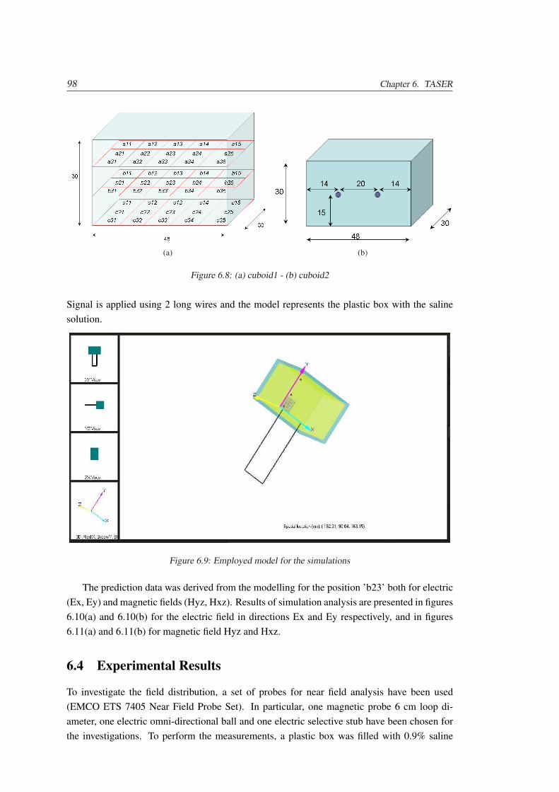
98 Chapter 6. TASER
(a) (b)
Figure 6.8: (a) cuboid1 - (b) cuboid2
Signal is applied using 2 long wires and the model represents the plastic box with the salinesolution.
Figure 6.9: Employed model for the simulations
The prediction data was derived from the modelling for the position ’b23’ both for electric(Ex, Ey) and magnetic fields (Hyz, Hxz). Results of simulation analysis are presented in figures6.10(a) and 6.10(b) for the electric field in directions Ex and Ey respectively, and in figures6.11(a) and 6.11(b) for magnetic field Hyz and Hxz.
6.4 Experimental Results
To investigate the field distribution, a set of probes for near field analysis have been used(EMCO ETS 7405 Near Field Probe Set). In particular, one magnetic probe 6 cm loop di-ameter, one electric omni-directional ball and one electric selective stub have been chosen forthe investigations. To perform the measurements, a plastic box was filled with 0.9% saline
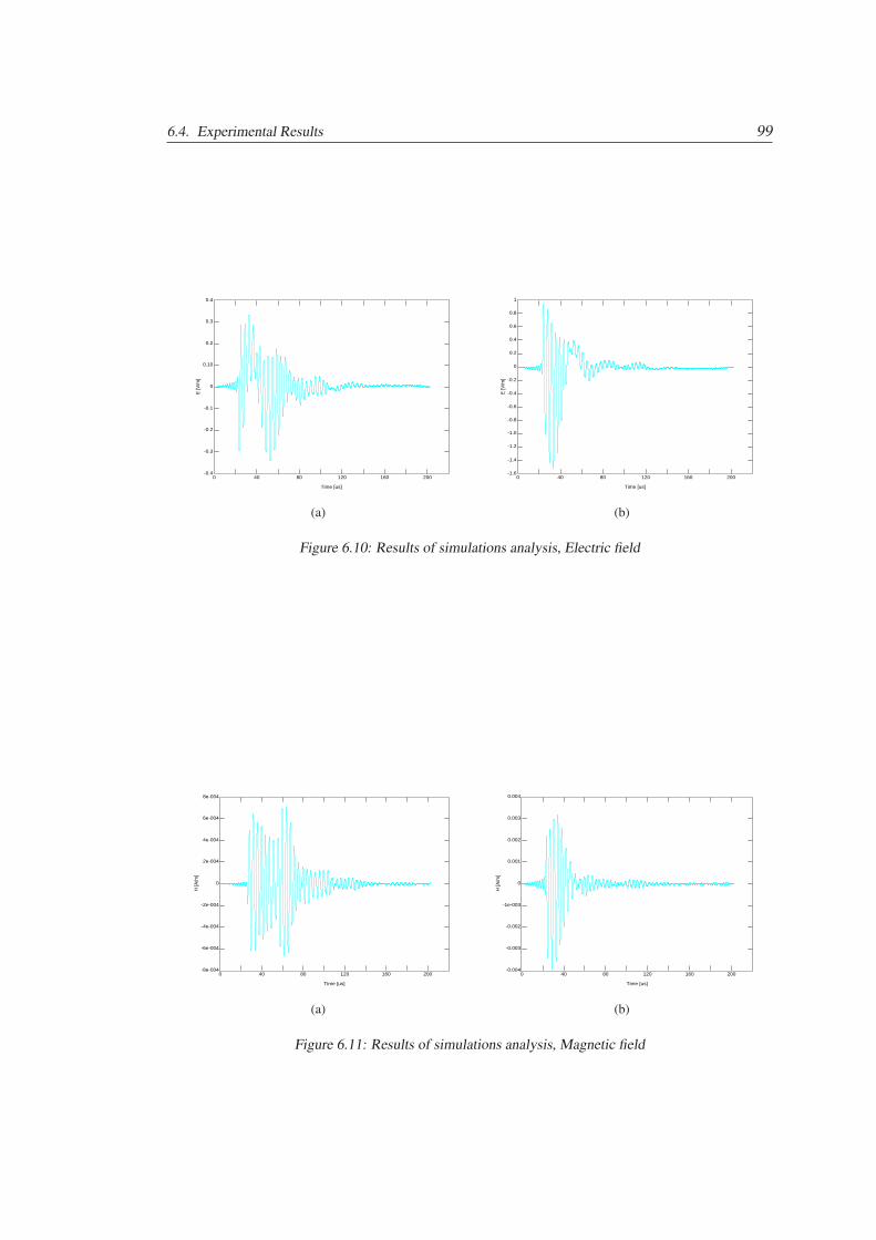
6.4. Experimental Results 99
0 40 80 120 160 200-0.4
-0.3
-0.2
-0.1
0
0.10
0.2
0.3
0.4
Time [us]
E [V
/m]
(a)
0 40 80 120 160 200-1.6
-1.4
-1.2
-1.0
-0.8
-0.6
-0.4
-0.2
0
0.2
0.4
0.6
0.8
1
Time [us]
E [V
/m]
(b)
Figure 6.10: Results of simulations analysis, Electric field
0 40 80 120 160 200-8e-004
-6e-004
-4e-004
-2e-004
0
2e-004
4e-004
6e-004
8e-004
Time [us]
H [A
/m]
(a)
0 40 80 120 160 200-0.004
-0.003
-0.002
-1e-003
0
0.001
0.002
0.003
0.004
Time [us]
H [A
/m]
(b)
Figure 6.11: Results of simulations analysis, Magnetic field
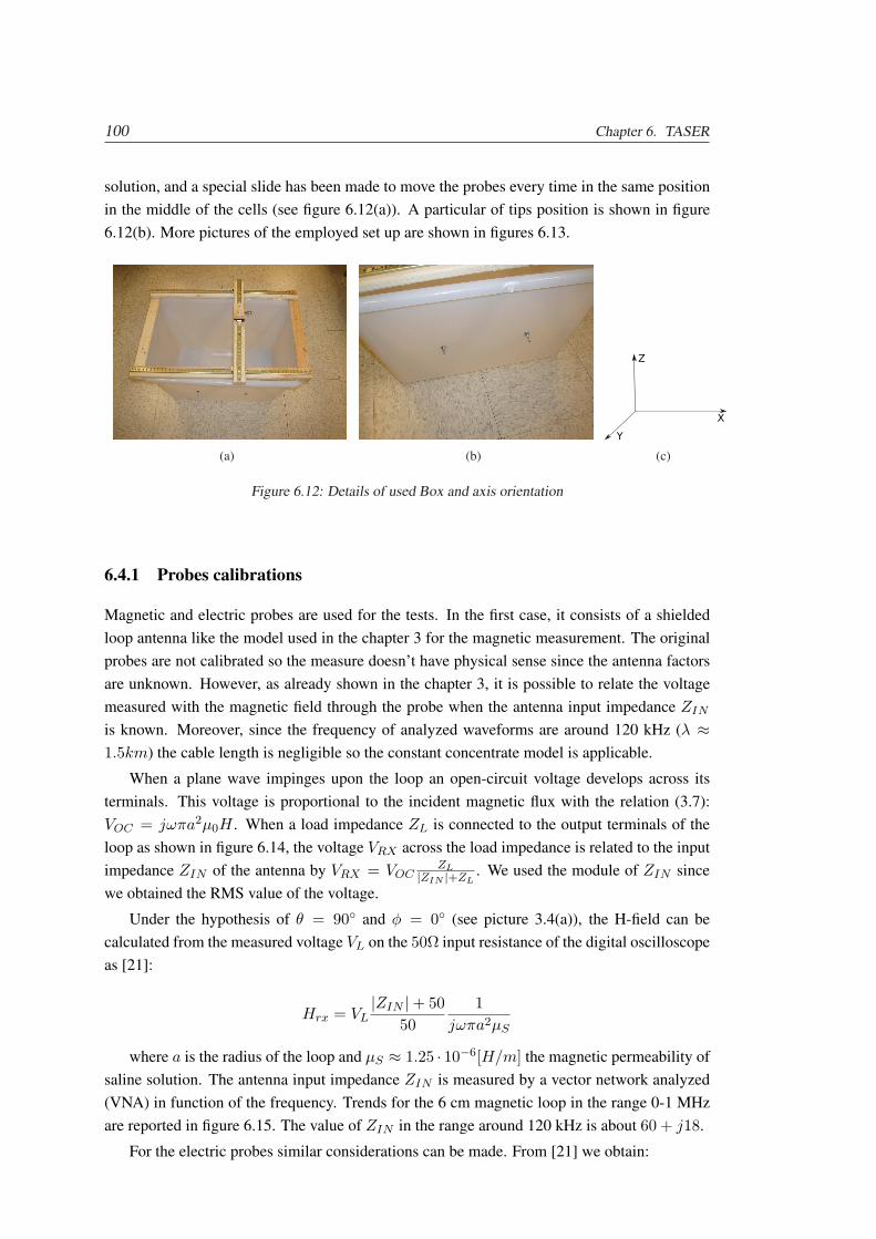
100 Chapter 6. TASER
solution, and a special slide has been made to move the probes every time in the same positionin the middle of the cells (see figure 6.12(a)). A particular of tips position is shown in figure6.12(b). More pictures of the employed set up are shown in figures 6.13.
(a) (b) (c)
Figure 6.12: Details of used Box and axis orientation
6.4.1 Probes calibrations
Magnetic and electric probes are used for the tests. In the first case, it consists of a shieldedloop antenna like the model used in the chapter 3 for the magnetic measurement. The originalprobes are not calibrated so the measure doesn’t have physical sense since the antenna factorsare unknown. However, as already shown in the chapter 3, it is possible to relate the voltagemeasured with the magnetic field through the probe when the antenna input impedance ZIN
is known. Moreover, since the frequency of analyzed waveforms are around 120 kHz (λ ≈1.5km) the cable length is negligible so the constant concentrate model is applicable.
When a plane wave impinges upon the loop an open-circuit voltage develops across itsterminals. This voltage is proportional to the incident magnetic flux with the relation (3.7):VOC = jωπa2µ0H . When a load impedance ZL is connected to the output terminals of theloop as shown in figure 6.14, the voltage VRX across the load impedance is related to the inputimpedance ZIN of the antenna by VRX = VOC
ZL|ZIN |+ZL
. We used the module of ZIN sincewe obtained the RMS value of the voltage.
Under the hypothesis of θ = 90 and φ = 0 (see picture 3.4(a)), the H-field can becalculated from the measured voltage VL on the 50Ω input resistance of the digital oscilloscopeas [21]:
Hrx = VL|ZIN |+ 50
501
jωπa2µS
where a is the radius of the loop and µS ≈ 1.25 · 10−6[H/m] the magnetic permeability ofsaline solution. The antenna input impedance ZIN is measured by a vector network analyzed(VNA) in function of the frequency. Trends for the 6 cm magnetic loop in the range 0-1 MHzare reported in figure 6.15. The value of ZIN in the range around 120 kHz is about 60 + j18.
For the electric probes similar considerations can be made. From [21] we obtain:
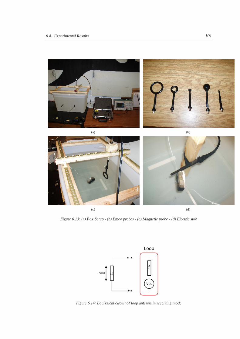
6.4. Experimental Results 101
(a) (b)
(c) (d)
Figure 6.13: (a) Box Setup - (b) Emco probes - (c) Magnetic probe - (d) Electric stub
Figure 6.14: Equivalent circuit of loop antenna in receiving mode
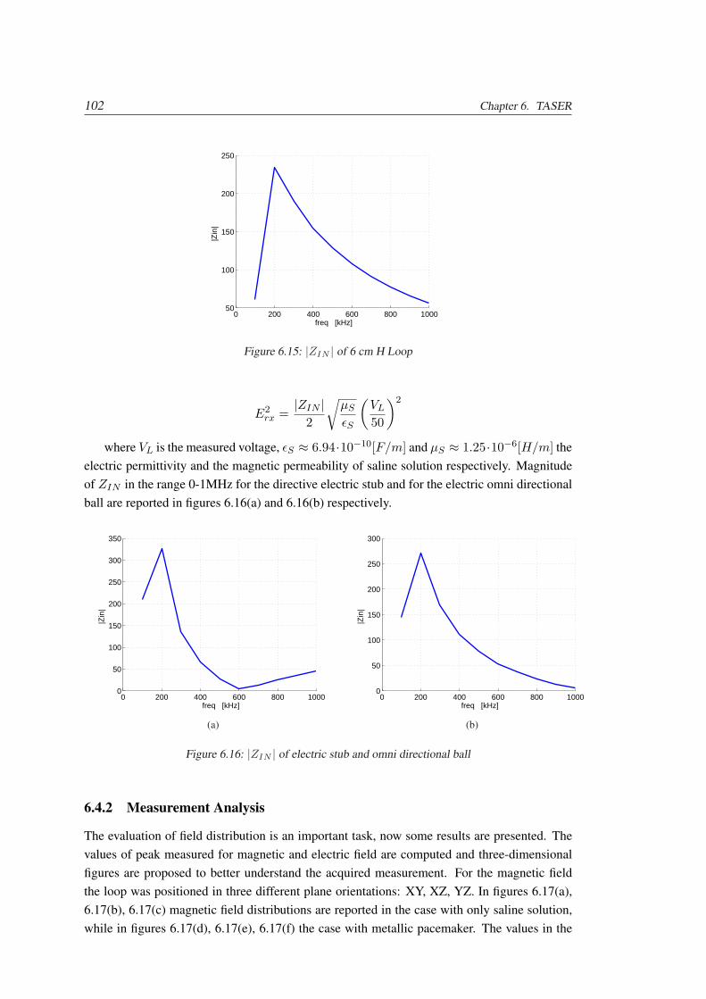
102 Chapter 6. TASER
0 200 400 600 800 100050
100
150
200
250
freq [kHz]
|Zin
|
Figure 6.15: |ZIN | of 6 cm H Loop
E2rx =
|ZIN |2
õS
εS
(VL
50
)2
where VL is the measured voltage, εS ≈ 6.94·10−10[F/m] and µS ≈ 1.25·10−6[H/m] theelectric permittivity and the magnetic permeability of saline solution respectively. Magnitudeof ZIN in the range 0-1MHz for the directive electric stub and for the electric omni directionalball are reported in figures 6.16(a) and 6.16(b) respectively.
0 200 400 600 800 10000
50
100
150
200
250
300
350
freq [kHz]
|Zin
|
(a)
0 200 400 600 800 10000
50
100
150
200
250
300
freq [kHz]
|Zin
|
(b)
Figure 6.16: |ZIN | of electric stub and omni directional ball
6.4.2 Measurement Analysis
The evaluation of field distribution is an important task, now some results are presented. Thevalues of peak measured for magnetic and electric field are computed and three-dimensionalfigures are proposed to better understand the acquired measurement. For the magnetic fieldthe loop was positioned in three different plane orientations: XY, XZ, YZ. In figures 6.17(a),6.17(b), 6.17(c) magnetic field distributions are reported in the case with only saline solution,while in figures 6.17(d), 6.17(e), 6.17(f) the case with metallic pacemaker. The values in the
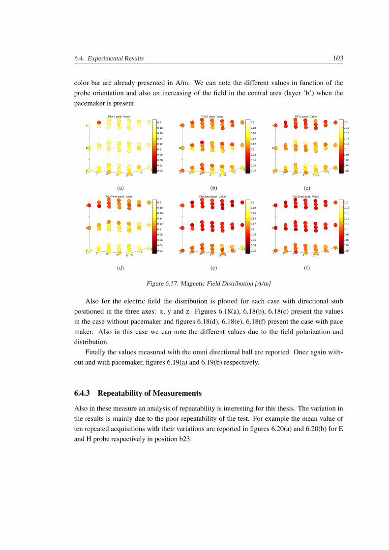
6.4. Experimental Results 103
color bar are already presented in A/m. We can note the different values in function of theprobe orientation and also an increasing of the field in the central area (layer ’b’) when thepacemaker is present.
12
31 2 3 4 5
c
b
a
P6XY peak Value
0.02
0.04
0.06
0.08
0.1
0.12
0.14
0.16
0.18
0.2
(a)
12
31 2 3 4 5
c
b
a
P6XZ peak Value
0.02
0.04
0.06
0.08
0.1
0.12
0.14
0.16
0.18
0.2
(b)
12
31 2 3 4 5
c
b
a
P6YZ peak Value
0.02
0.04
0.06
0.08
0.1
0.12
0.14
0.16
0.18
0.2
(c)
12
31 2 3 4 5
c
b
a
P6XYmet peak Value
0.02
0.04
0.06
0.08
0.1
0.12
0.14
0.16
0.18
0.2
(d)
12
31 2 3 4 5
c
b
a
P6XZmet peak Value
0.02
0.04
0.06
0.08
0.1
0.12
0.14
0.16
0.18
0.2
(e)
12
31 2 3 4 5
c
b
a
P6YZmet peak Value
0.02
0.04
0.06
0.08
0.1
0.12
0.14
0.16
0.18
0.2
(f)
Figure 6.17: Magnetic Field Distribution [A/m]
Also for the electric field the distribution is plotted for each case with directional stubpositioned in the three axes: x, y and z. Figures 6.18(a), 6.18(b), 6.18(c) present the valuesin the case without pacemaker and figures 6.18(d), 6.18(e), 6.18(f) present the case with pacemaker. Also in this case we can note the different values due to the field polarization anddistribution.
Finally the values measured with the omni directional ball are reported. Once again with-out and with pacemaker, figures 6.19(a) and 6.19(b) respectively.
6.4.3 Repeatability of Measurements
Also in these measure an analysis of repeatability is interesting for this thesis. The variation inthe results is mainly due to the poor repeatability of the test. For example the mean value often repeated acquisitions with their variations are reported in figures 6.20(a) and 6.20(b) for Eand H probe respectively in position b23.
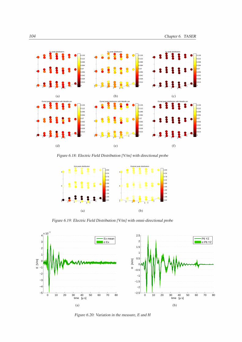
104 Chapter 6. TASER
12
31 2 3 4 5
c
b
a
Ex peak distribution
0
0.014
0.028
0.042
0.056
0.07
0.084
0.098
0.112
0.126
(a)
12
31 2 3 4 5
c
b
a
Ey peak distribution
0
0.014
0.028
0.042
0.056
0.07
0.084
0.098
0.112
0.126
(b)
12
31 2 3 4 5
c
b
a
Ez peak distribution
0
0.014
0.028
0.042
0.056
0.07
0.084
0.098
0.112
0.126
(c)
12
31 2 3 4 5
c
b
a
Exmet peak distribution with Metallic pm
0
0.014
0.028
0.042
0.056
0.07
0.084
0.098
0.112
0.126
(d)
12
31 2 3 4 5
c
b
a
Eymet peak distribution with Metallic pm
0
0.014
0.028
0.042
0.056
0.07
0.084
0.098
0.112
0.126
(e)
12
31 2 3 4 5
c
b
a
Ezmet peak distribution with Metallic pm
0
0.014
0.028
0.042
0.056
0.07
0.084
0.098
0.112
0.126
(f)
Figure 6.18: Electric Field Distribution [V/m] with directional probe
12
31 2 3 4 5
c
b
a
Etot peak distribution
0.64
1.09
1.54
1.99
2.44
2.89
3.34
3.79
4.24
4.69
(a)
12
31 2 3 4 5
c
b
a
Etotmet peak distribution
0.64
1.09
1.54
1.99
2.44
2.89
3.34
3.79
4.24
4.69
(b)
Figure 6.19: Electric Field Distribution [V/m] with omni-directional probe
0 10 20 30 40 50 60 70 80−5
−4
−3
−2
−1
0
1
2
3
4x 10
−3
time [µ s]
E [
V/m
]
Ex meanσ Ex
(a)
0 10 20 30 40 50 60 70 80−2.5
−2
−1.5
−1
−0.5
0
0.5
1
1.5
2
2.5
time [µ s]
H
[A/m
]
P6 YZσ P6 YZ
(b)
Figure 6.20: Variation in the measure, E and H
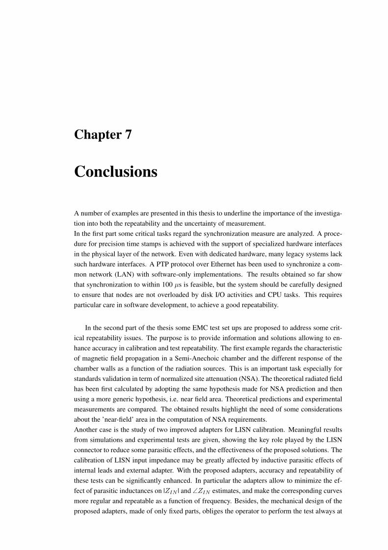
Chapter 7
Conclusions
A number of examples are presented in this thesis to underline the importance of the investiga-tion into both the repeatability and the uncertainty of measurement.In the first part some critical tasks regard the synchronization measure are analyzed. A proce-dure for precision time stamps is achieved with the support of specialized hardware interfacesin the physical layer of the network. Even with dedicated hardware, many legacy systems lacksuch hardware interfaces. A PTP protocol over Ethernet has been used to synchronize a com-mon network (LAN) with software-only implementations. The results obtained so far showthat synchronization to within 100 µs is feasible, but the system should be carefully designedto ensure that nodes are not overloaded by disk I/O activities and CPU tasks. This requiresparticular care in software development, to achieve a good repeatability.
In the second part of the thesis some EMC test set ups are proposed to address some crit-ical repeatability issues. The purpose is to provide information and solutions allowing to en-hance accuracy in calibration and test repeatability. The first example regards the characteristicof magnetic field propagation in a Semi-Anechoic chamber and the different response of thechamber walls as a function of the radiation sources. This is an important task especially forstandards validation in term of normalized site attenuation (NSA). The theoretical radiated fieldhas been first calculated by adopting the same hypothesis made for NSA prediction and thenusing a more generic hypothesis, i.e. near field area. Theoretical predictions and experimentalmeasurements are compared. The obtained results highlight the need of some considerationsabout the ’near-field’ area in the computation of NSA requirements.Another case is the study of two improved adapters for LISN calibration. Meaningful resultsfrom simulations and experimental tests are given, showing the key role played by the LISNconnector to reduce some parasitic effects, and the effectiveness of the proposed solutions. Thecalibration of LISN input impedance may be greatly affected by inductive parasitic effects ofinternal leads and external adapter. With the proposed adapters, accuracy and repeatability ofthese tests can be significantly enhanced. In particular the adapters allow to minimize the ef-fect of parasitic inductances on |ZIN | and ∠ZIN estimates, and make the corresponding curvesmore regular and repeatable as a function of frequency. Besides, the mechanical design of theproposed adapters, made of only fixed parts, obliges the operator to perform the test always at

106 Chapter 7. Conclusions
the same physical conditions of test bench components.The repeatability contribution on the evaluation of uncertainty has also been analyzed for theair discharge tests. It has been shown that the type A uncertainty, which is not so importantfor contact ESD tests, becomes essential in the case of air ESD tests. In fact, if not adequatelycontrolled, it may lead to a relevant degradation of the test repeatability in an ESD generator.Conflicting requirements are provided about this issue in the available standards. This meansthat lab technicians might interpret such requirements in different ways, to the detriment ofthe test repeatability. To this aim, a proposal has been reported based on a specific device, tobe used for the control of the gun speed in air discharge tests. The uncertainty contributionassociated to the humidity variation during the tests performed within the climatic chamber isalso significant. It has been found that it must be below 2% with humidity variations lowerthan 1%.Finally, a set of measurements aimed to understand the field distribution when a TASER dis-charge affects a human body is presented. Selected results from proper simulations and exper-iments are proposed to confer reliability and generality to the research activity. Details con-cerning the test bed, which includes a purposely-developed system, measurement procedureand experiment are also provided.
Appendix A
Matlab code for theoretical fieldsevaluation
c l e a r a l lc l o s e a l l
% DATA INPUTa = 0 . 0 7 9 6 ; % r a d i u s o f Tx loop [m]b = 0 . 0 7 9 6 ; % r a d i u s o f Rx an tenna [m]f r e q =60; % MHzI = 1 6 / ( 5 2 . 1 8∗ s q r t ( 2 ) ∗ 2 ) ; % c u r r e n t [A RMS]D=3; % a n t e n n a s ’ d i s t a n c e [ mt ]h2 = [ 1 : 0 . 2 : 3 ] ; % Rx an tenna h e i g h t 1−3 mtZrx = 9 3 . 7 7 5 ; %| Z | Rx an tennaa t t = 1 0 ; % a t t e n u a t i o n a t Rx o u t [ dB ]measureyz =[−78.10 ,−78.54 ,−78.66 ,−78.90 ,−78.99 ,−79.05 ,
−79.18 ,−79.33 ,−79.56 ,−79.91 ,−80.30] ;measurexy =[−78.31 ,−77.00 ,−75.43 ,−75.20 ,−74.88 ,−74.82 ,
−74.80 ,−74.82 ,−75.29 ,−75.70 ,−76.40] ;measurexz =[−76.32 ,−75.53 ,−74.74 ,−74.35 ,−73.84 ,−73.65 ,
−73.88 ,−73.68 ,−74.02 ,−74.56 ,−75.05] ;
l ung =300/ f r e q ; % w a v e l e n g h t [m]k=2∗ pi / l ung ; % wave number
% ( Y−Z ) Planemeasureyz = measureyz + a t t ;h1 = 1 . 1 ; % Tx an tenna h e i g h td1 =(D^2+( h1−h2 ) . ^ 2 ) . ^ 0 . 5 ; % d i s t a n c e f o r d i r e c t wavesd2 =(D^2+( h1+h2 ) . ^ 2 ) . ^ 0 . 5 ; % d i s t a n c e f o r r e f l e c t e d wavesQ1= pi / 2 ; % t h e t a 1Q2= pi / 2 ; % t h e t a 2
H1r= j ∗ ( k∗a ^2∗ I ∗ cos ( Q1 ) ) . / ( 2 ∗ d1 . ^ 2 ) . ∗ ( 1 + 1 . / ( j ∗k .∗ d1 ) ) . ∗ exp(− j ∗k .∗ d1 ) ;H2r= j ∗ ( k∗a ^2∗ I ∗ cos ( Q2 ) ) . / ( 2 ∗ d2 . ^ 2 ) . ∗ ( 1 + 1 . / ( j ∗k .∗ d2 ) ) . ∗ exp(− j ∗k .∗ d2 ) ;
H1Q=−((k∗a )^2∗ I ∗ s i n ( Q1 ) ) . / ( 4 ∗ d1 ) . ∗ ( 1 + 1 . / ( j ∗k .∗ d1 ) −1 . / ( k .∗ d1 ) . ^ 2 )
108 Appendix A. Matlab code for theoretical fields evaluation
.∗ exp(− j ∗k .∗ d1 ) ;H2Q=−((k∗a )^2∗ I ∗ s i n ( Q2 ) ) . / ( 4 ∗ d2 ) . ∗ ( 1 + 1 . / ( j ∗k .∗ d2 ) −1 . / ( k .∗ d2 ) . ^ 2 )
.∗ exp(− j ∗k .∗ d2 ) ;
Hr=H1r+H2r ;HQ=H1Q+H1Q;
Hto t =abs ( Hr+HQ) ; % t h e o r i c a l H− f i e l d r e c e i v e dVoc= s q r t ( ( ( 1 0 . ^ ( measureyz . / 1 0 ) ) . / 1 0 0 0 ) . ∗ 5 0 ) ; % v o l t a g e a t Rx loo p t e r m i n a lHmeas=Voc . / ( ( b∗b∗pi )∗ ( 4∗ pi ∗0 . 0000 001 )
∗ (2∗ pi ∗ f r e q ∗1 0 0 0 0 0 0 ) ) ; % H− f i e l d i m p i n g i n g upon t h e loope r r =Htot−Hmeas ; % e r r o r be tween t h e o r i c a l and p r a c t i c a l r e s u l t s
f i g u r e ( ’ name ’ , ’ | H | ’ ) ;s e t ( gca , ’ F o n t S i z e ’ , 1 2 ) ;t i t l e ( ’Y−Z p l a n e @ 60MHz’ ) ;hold on ;gr id ;p l o t ( h2 , Htot , h2 , Hmeas , ’ o ’ ) ;x l a b e l ( ’ \ f o n t s i z e 12 h2 [m] ’ ) ;y l a b e l ( ’ \ f o n t s i z e 12 | H | [A/m] ’ ) ;hold o f fpause ;
f i g u r e ( ’ name ’ , ’ measured | H | ’ ) ;s e t ( gca , ’ F o n t S i z e ’ , 1 2 ) ;t i t l e ( ’Y−Z p l a n e @ 60MHz’ ) ;hold on ;gr id ;p l o t ( h2 , Hmeas ) ;x l a b e l ( ’ \ f o n t s i z e 12 h2 [m] ’ ) ;y l a b e l ( ’ \ f o n t s i z e 12 | H | Rx ’ ) ;hold o f fpause ;
f i g u r e ( ’ name ’ , ’ E r r o r Y−Z ’ ) ;s e t ( gca , ’ F o n t S i z e ’ , 1 2 ) ;t i t l e ( ’Y−Z P l a n e @ 60MHz’ ) ;hold on ;gr id ;p l o t ( h2 , e r r ) ;x l a b e l ( ’ \ f o n t s i z e 12 h2 [m] ’ ) ;y l a b e l ( ’ \ f o n t s i z e 12 gap [dBm] ’ ) ;hold o f fpause ;
% ( X−Y ) Planemeasurexy=measurexy+ a t t ;h1 = 0 . 9 8 5 ; % Tx an tenna h e i g h td1 =(D^2+( h1−h2 ) . ^ 2 ) . ^ 0 . 5 ; % d i s t a n c e f o r d i r e c t wavesd2 =(D^2+( h1+h2 ) . ^ 2 ) . ^ 0 . 5 ; % d i s t a n c e f o r r e f l e c t e d waves
109
Q1= a s i n (D . / d1 ) ; % t e t a 1Q2= a s i n (D . / d2 ) ; % t e t a 2
H1r= j ∗ ( k∗a ^2∗ I ∗ cos ( Q1 ) ) . / ( 2 ∗ d1 . ^ 2 ) . ∗ ( 1 + 1 . / ( j ∗k .∗ d1 ) ) . ∗ exp(− j ∗k .∗ d1 ) ;H2r= j ∗ ( k∗a ^2∗(− I )∗ cos (Q2 ) ) . / ( 2 ∗ d2 . ^ 2 ) . ∗ ( 1 + 1 . / ( j ∗k .∗ d2 ) ) . ∗ exp(− j ∗k .∗ d2 ) ;
H1Q=−((k∗a )^2∗ I ∗ s i n ( Q1 ) ) . / ( 4 ∗ d1 ) . ∗ ( 1 + 1 . / ( j ∗k .∗ d1 ) −1 . / ( k .∗ d1 ) . ^ 2 ).∗ exp(− j ∗k .∗ d1 ) ;
H2Q=−((k∗a )^2∗(− I )∗ s i n (Q2 ) ) . / ( 4 ∗ d2 ) . ∗ ( 1 + 1 . / ( j ∗k .∗ d2 ) −1 . / ( k .∗ d2 ) . ^ 2 ).∗ exp(− j ∗k .∗ d2 ) ;
H1z=H1r .∗ cos ( Q1)−H1Q.∗ s i n ( Q1 ) ;H2z=H2r .∗ cos ( Q1)−H2Q.∗ s i n ( Q2 ) ;
H to t =abs ( Hr+HQ) ; % t h e o r i c a l H− f i e l d r e c e i v e dVoc= s q r t ( ( ( 1 0 . ^ ( measureyz . / 1 0 ) ) . / 1 0 0 0 ) . ∗ 5 0 ) ; % v o l t a g e a t Rx loo p t e r m i n a lHmeas=Voc . / ( ( b∗b∗pi )∗ ( 4∗ pi ∗0.0000001
)∗ ( 2∗ pi ∗ f r e q ∗1 0 0 0 0 0 0 ) ) ; % H− f i e l d i m p i n g i n g upon t h e lo ope r r =Htot−Hmeas ; % e r r o r be tween t h e o r i c a l and p r a c t i c a l r e s u l t s
f i g u r e ( ’ name ’ , ’ | H | ’ ) ;s e t ( gca , ’ F o n t S i z e ’ , 1 2 ) ;t i t l e ( ’X−Y p l a n e @ 60MHz’ ) ;hold on ;gr id ;p l o t ( h2 , Htot , h2 , Hmeas , ’ o ’ ) ;x l a b e l ( ’ \ f o n t s i z e 12 h2 [m] ’ ) ;y l a b e l ( ’ \ f o n t s i z e 12 | H | [A/m] ’ ) ;hold o f fpause ;
f i g u r e ( ’ name ’ , ’ measured | H | ’ ) ;s e t ( gca , ’ F o n t S i z e ’ , 1 2 ) ;t i t l e ( ’X−Y p l a n e @ 60MHz’ ) ;hold on ;gr id ;p l o t ( h2 , Hmeas ) ;x l a b e l ( ’ \ f o n t s i z e 12 h2 [m] ’ ) ;y l a b e l ( ’ \ f o n t s i z e 12 | H | Rx ’ ) ;hold o f fpause ;
f i g u r e ( ’ name ’ , ’ E r r o r X−Y’ ) ;s e t ( gca , ’ F o n t S i z e ’ , 1 2 ) ;t i t l e ( ’X−Y P l a n e @ 60MHz’ ) ;hold on ;gr id ;p l o t ( h2 , e r r ) ;x l a b e l ( ’ \ f o n t s i z e 12 h2 [m] ’ ) ;y l a b e l ( ’ \ f o n t s i z e 12 gap [dBm] ’ ) ;hold o f fpause ;
110 Appendix A. Matlab code for theoretical fields evaluation
%( X−Z ) Planemeasurexz = measurexz + a t t ;h1 = 1 . 1 ; %Tx an tenna h e i g h td1 =(D^2+( h1−h2 ) . ^ 2 ) . ^ 0 . 5 ; %d i s t a n c e f o r d i r e c t wavesd2 =(D^2+( h1+h2 ) . ^ 2 ) . ^ 0 . 5 ; %d i s t a n c e f o r r e f l e c t e d wavesQ1= a s i n ( ( h2−h1 ) . / d1 ) ; %t e t a 1Q2= a s i n ( ( h2+h1 ) . / d2 ) ; %t e t a 2
H1r= j ∗ ( k∗a ^2∗ I ∗ cos ( Q1 ) ) . / ( 2 ∗ d1 . ^ 2 ) . ∗ ( 1 + 1 . / ( j ∗k .∗ d1 ) ) . ∗ exp(− j ∗k .∗ d1 ) ;H2r= j ∗ ( k∗a ^2∗ I ∗ cos ( Q2 ) ) . / ( 2 ∗ d2 . ^ 2 ) . ∗ ( 1 + 1 . / ( j ∗k .∗ d2 ) ) . ∗ exp(− j ∗k .∗ d2 ) ;
H1Q=−((k∗a )^2∗ I ∗ s i n ( Q1 ) ) . / ( 4 ∗ d1 ) . ∗ ( 1 + 1 . / ( j ∗k .∗ d1 ) −1 . / ( k .∗ d1 ) . ^ 2 ).∗ exp(− j ∗k .∗ d1 ) ;
H2Q=−((k∗a )^2∗ I ∗ s i n ( Q2 ) ) . / ( 4 ∗ d2 ) . ∗ ( 1 + 1 . / ( j ∗k .∗ d2 ) −1 . / ( k .∗ d2 ) . ^ 2 ).∗ exp(− j ∗k .∗ d2 ) ;
H1z=H1r .∗ cos ( Q1)−H1Q.∗ s i n ( Q1 ) ;H2z=H2r .∗ cos ( Q1)−H2Q.∗ s i n ( Q2 ) ;
H to t =abs ( Hr+HQ) ; %t h e o r i c a l H− f i e l d r e c e i v e dVoc= s q r t ( ( ( 1 0 . ^ ( measureyz . / 1 0 ) ) . / 1 0 0 0 ) . ∗ 5 0 ) ; % v o l t a g e a t Rx loo p t e r m i n a lHmeas=Voc . / ( ( b∗b∗pi )∗ ( 4∗ pi ∗0 . 0000 001 )
∗ (2∗ pi ∗ f r e q ∗1 0 0 0 0 0 0 ) ) ; %H− f i e l d i m p i n g i n g upon t h e loope r r =Htot−Hmeas ; %e r r o r be tween t h e o r i c a l and p r a c t i c a l r e s u l t s
f i g u r e ( ’ name ’ , ’ | H | ’ ) ;s e t ( gca , ’ F o n t S i z e ’ , 1 2 ) ;t i t l e ( ’X−Z p l a n e @ 60MHz’ ) ;hold on ;gr id ;p l o t ( h2 , Htot , h2 , Hmeas , ’ o ’ ) ;x l a b e l ( ’ \ f o n t s i z e 12 h2 [m] ’ ) ;y l a b e l ( ’ \ f o n t s i z e 12 | H | [A/m] ’ ) ;hold o f fpause ;
f i g u r e ( ’ name ’ , ’ measured | H | ’ ) ;s e t ( gca , ’ F o n t S i z e ’ , 1 2 ) ;t i t l e ( ’X−Z p l a n e @ 60MHz’ ) ;hold on ;gr id ;p l o t ( h2 , Hmeas ) ;x l a b e l ( ’ \ f o n t s i z e 12 h2 [m] ’ ) ;y l a b e l ( ’ \ f o n t s i z e 12 | H | Rx ’ ) ;hold o f fpause ;
f i g u r e ( ’ name ’ , ’ E r r o r X−Z ’ ) ;s e t ( gca , ’ F o n t S i z e ’ , 1 2 ) ;t i t l e ( ’X−Z P l a n e @ 60MHz’ ) ;hold on ;

111
gr id ;p l o t ( h2 , e r r ) ;x l a b e l ( ’ \ f o n t s i z e 12 h2 [m] ’ ) ;y l a b e l ( ’ \ f o n t s i z e 12 gap [dBm] ’ ) ;hold o f fpause ;


Bibliography
[1] ISO GUM, Guide to the Expression of Uncertainty in Measurement, Ed. 1, 1995. Interna-tional Organisation for Standardisation, Geneva (Switzerland).
[2] Barry N. Taylor, Chris E. Kuyatt Guidelines for Evaluating and Expressing the Uncertaintyof NIST Measurement Results, NIST First Ed.
[3] www.acmesystems.it
[4] D.L. Mills, “Network Time Protocol (Version 3) Specification, Implementation and Anal-ysis”, RFC 1305, Internet Engineering Task Force Network Working Group.
[5] N. M. Freris, P. R. Kumar, “Fundamental Limits on synchronization of Affine clocks inNetworks”, Proc. of the 46th IEEE Conference on Decision and Control, New Orleans,USA, Dec. 12-14, 2007.
[6] IEEE 1588TM 2002, “Standard for a Precision Clock Synchronization Protocol for Net-worked Measurement and control Systems”.
[7] G. Giorgi, C. Narduzzi, “Modeling and Simulation Analysis of PTP Clock Servo”, Proc.of ISPCS2007 Symposium, Vienna, austria, October 1-3, 2007, pp. 155-161.
[8] Endace: http://www.endace.com.
[9] L. Benetazzo, C. Narduzzi, M. Stellini, “Analysis of clock tracking performances for asoftware-only IEEE 1588 implemetation”, Proc. of the Instr. Meas. Tech. Conf. IMTC2007,Warsaw, Poland, May 1-3, 2007.
[10] W. Leland, M. Taqqu, W. Willinger, D. Wilson, “On the Self-Similar Nature of EthernetTraffic”, IEEE/ACM Transaction on Networking, vol. 2, February 1994, pp. 1-15.
[11] A. Erramilli, R. P. Singh, P. Pruthi, “Chaotic maps as models of packet traffic”, Proc. ITC14. the Fundamental Role of Teletraffic in the Evolution of Telecommunication Networks,1994, pp. 329-338.
[12] P. Abry, D. Veitch, “Wavelet analysis of long-range-dependent traffic”, IEEE Transac-tions on Information Theory, vol. 44. n. 1, 1998, pp. 2-15.
[13] D. L. Mills, P. H. Kamp, “The Nanokernel”, Proc. of the Precision Time and Time Interval(PTTI) Applications and Planning Meeting, 2000.

114 Bibliography
[14] K. Correll, N. Barendt, M. Branicky, “Design Considerations for Software Only Imple-mentations of the IEEE 1588 Precision Time Protocol”, Proc. of the 2005 Conference onIEEE 1588, Zurich, Switzerland, October 10-12, 2005.
[15] EN 50081-1:1992 and -2:1993, Electromagnetic compatibility - Generic emission stan-dard, BSI, 1992
[16] EN 50081-1:1997 (second edition) and -2:1995, Electromagnetic compatibility - Genericimmunity standard, BSI, 1997
[17] CISPR 16-2-3 (edition 2.0), Specification for radio disturbance and immunity measuringapparatus and methods - Part 2-3: Methods of measurement of disturbances and immunity- Radiated disturbance measurements, July 2006
[18] CISPR 16-1-4 (edition 2.0) Specification for radio disturbance and immunity measuringapparatus and methods - Part 1-4: Radio disturbance and immunity measuring apparatus -Ancillary equipment - Radiated disturbances, Oct. 2007
[19] H.F. Garn, E. Zink, W. Mullwer, R. Kremser, A new Instrument for the Determinationof Product-Specific Chamber Factors for Radiated-Emissions Tests, EMC Zurich 1993, pp.93-98.
[20] CENELEC Technical Report R210-003, Guidelines on how to use anechoic enclosurethat do not fulfil the requirements regarding normalized site attenuation for pre-compliancetests of products, Nov. 1995.
[21] Constantine A. Balanis, Antenna Theory, -analysis and desing- - Wiley- Interscince, 3thed.
[22] A.A. Smith, Jr., R.F. German, and J.B. Pate, Calculation of site attenuation from antennafactors, IEEE Trans. Electr. Comp. vol. EMC-24, pp. 301-316, 1982.
[23] Michele Borsero, Andrea Dalla Chiara, Claudio Pravato, Alessandro Sona, MarcoStellini, Alessandro Zuccato. Cosiderations about Radiated Emission Tests in AnechoicChamber that do not fullfill the NSA Requirements, IMEKO TC4 Symposium, 2008.
[24] Tim Williams: EMC for product designer, (second edition) BH NewNes, 1996.
[25] Clayton R. Paul: Introduction to Electromagnetic Compatibility, John Wiley & Sons,1992.
[26] CISPR 16-1-2: 2006, Specification for radio disturbance and immunity measuring ap-paratus and methods. Part 1.2: Radio disturbance and immunity measuring apparatus -Ancillary equipment - Conducted disturbances, IEC, Ginevra.
[27] Bronaugh E. L., Mains Simulation Network (LISN or AMN) Uncertainty - How Goodare Your Conducted Emission Measurements ?, EMC International Zurich Symposium onEMC, Zurich, February 1999, pp. 521 - 526.

Bibliography 115
[28] Zuccato A., Tomasin P., Florean D., Undesired Uncertainty in Conducted Full-Compliance Measurement: A Proposal for Verification of Conformity of LISN ParametersAccording to Requirements of CISPR16-1. IEEE International Symposium on EMC, Mon-treal, August 2001. Volume 1, pp. 7-12.
[29] International Standard - IEC 61000-4-6 Electromagnetic compatibility (EMC) - Testingand measurement techniques - Immunity to conducted disturbances, induced by radio-frequency fields Basic EMC publication (Ed. 2000).
[30] IEC, Std 61000-4-2, Electromagnetic Compatibility (EMC), Part 4: Testing and measure-ment techniques - Section 2: Electrostatic discharge immuty test, Ed. 1.2, 2001.
[31] ISO, Std 10605, Road vehicles - Test methods for electrical disturbances from electro-static discharge, 2001.
[32] K. Hilty, H. Ryser, U. Herrmann, Calibration of Electrostaic Dischareg Generators andresults of an International Comparison, IEEE Trans. on Instrumentation and Measurement,vol. 50, no. 2, Apr. 2001, pp. 414-418.
[33] K. Tae-Weon, C. Yeon-Choon, W. Sung-Ho, K. Hyo-Tae, On the Uncertainty in the Cur-rent Waveform Measurement of an ESD Generator, IEEE Trans. on EMC, vol. 42, no. 4,Nov. 2000, pp. 405-413.
[34] P. Richman, Classification of ESD hand/metal current waves versus approach speed, volt-age, electrode geometry and humidity, Proc. IEEE Int. Symp. EMC, 1986, pp. 451-460.
[35] J.S. Maas and D.J. Pratt, A study of the repeatability of electrostatic discharge simulator,Proc. IEEE Int. Symp. EMC, 1990, pp. 265-269.
[36] M. Mardiguian, Electrostatic Discharge, Interference Control Technologies, Gainsville,Virginia, 1986.
[37] S.Caniggia, F. Maradei, Circuit and Numerical Modeling of Electrostatic Discharge Gen-erators, IEEE Trans. On Industry Application, Vol.42, No.6, November/December 2006.
[38] S.J. Holden, R.D. Sheridan, T.J. Coffey, R.A. Scaramuzza and P. Diamantopoulos, Elec-tromagnetic modelling of current flow in the heart from TASER devices and the risk of car-diac dysrhythmias, Phys. Med. Biol. 52 (2007) 7193-7209.
[39] Taser official web site, www.taser.com