Evaluating the Effectiveness of Regression Testing

Master of Science Thesis Software Engineering and Technology

MEHVISH RASHID

Chalmers University of TechnologyUniversity of GothenburgDepartment of Computer Science and EngineeringGöteborg, Sweden, February 2011

The Author grants to Chalmers University of Technology and University of Gothenburg the non-exclusive right to publish the Work electronically and in a non-commercial purpose make it accessible on the Internet.The Author warrants that he/she is the author to the Work, and warrants that the Work does not contain text, pictures or other material that violates copyright law.

The Author shall, when transferring the rights of the Work to a third party (for example a publisher or a company), acknowledge the third party about this agreement. If the Author has signed a copyright agreement with a third party regarding the Work, the Author warrants hereby that he/she has obtained any necessary permission from this third party to let Chalmers University of Technology and University of Gothenburg store the Work electronically and make it accessible on the Internet.

Evaluation of Regression Test Effectiveness , Industry based Master Thesis

© Mehvish Rashid, 2011.

Examiner: Robert Feldt

Chalmers University of TechnologyUniversity of GothenburgDepartment of Computer Science and EngineeringSE-412 96 GöteborgSwedenTelephone + 46 (0)31-772 1000

Cover: Figure 6: Test case i and j in a pair wise matrix each with pass denoted by 1 and fail by -1 and possible combinations of schemes derivation.

Department of Computer Science and EngineeringGöteborg, Sweden February 2011

Abstract

Regression testing is the retesting of a software to check its reliability against the new functionality that is implemented or changes are made to the software. Regression testing plays a significant role to assess the quality of a product that is changed frequently in functionality as expected by the end user of the software. There has been a number of studies on various regression testing techniques as mentioned by Yoo and Harman in their survey but a very few are dedicated to the evaluating regression testing techniques.

In this study various methods or schemes are suggested to measure the uniqueness of a test case. The uniqueness measure of a test case is a tool that is utilized to make decision on the effectiveness of various regression test techniques.

Finally, building blocks for the construction of a framework are provided in the form of various schemes classified by their level of complexity involved. Concepts and methods that are utilized are already proven by academia and literature that help to devise the schemes or methods in the conducted industrial study. The formulated schemes can be applied to the extracted information in the form of 0, 1's and -1's. The solution given here can be considered as a generalized one for a wide range of industry and academia to facilitate in the decision making with various kind of existing data situations.

Acknowledgment

The study was conducted with the cooperation of Ericsson AB, Karlskrona. I would like to thank Ericsson for their extended cooperation and guidance throughout the duration of the project. The purpose of the study conducted would have not been accomplished without the supervision of Dr. Robert Feldt from Chalmers University of Technology, I thank him with the depth of my heart.

Mehvish Rashid

Evaluating the Effectiveness of Regression Testing

Mehvish RashidChalmers University of Technology, Goteborg.

mehvish@student.chalmers.se, rmehvish@gmail.com

Abstract

Regression testing is the retesting of a software to check its reliability against the new functionality that is implemented or changes are made to the software. Regression testing plays a significant role to assess the quality of a product that is changed frequently in functionality as expected by the end user of the software. There has been a number of studies on various regression testing techniques as mentioned by Yoo and Harman in their survey but a very few are dedicated to the evaluating regression testing techniques.

In this study various methods or schemes are suggested to measure the uniqueness of a test case. The uniqueness measure of a test case is a tool that is utilized to make decision on the effectiveness of various regression test techniques.

Finally, building blocks for the construction of a framework are provided in the form of various schemes classified by their level of complexity involved. Concepts and methods that are utilized are already proven by academia and literature that help to devise the schemes or methods in the conducted industrial study. The formulated schemes can be applied to the extracted information in the form of 0, 1's and -1's. The solution given here can be considered as a generalized one for a wide range of industry and academia to facilitate in the decision making with various kind of existing data situations.

1. Introduction

Ericsson has been a world leader in Telecom Industry since 1876 providing telecommunication equipment, and related services to the mobile and fixed networks operators. The systems developed are to facilitate the mobile operators in more than 175 countries and more than 40 percent of the world’s mobile traffic passes through Ericsson networks. The systems are consistently tested for their quality standards while performing the regression testing.Regression testing is the process of retesting of a system or component to verify that changes made to the system code have not caused unintended effects and that the system is still compliant with the specified requirements [1]. Several techniques have been suggested in the literature such as Prioritization of Requirements for Test (PORT). PORT can be used to prioritize system-level black box test when traceability between requirements, test case, and test field failures is maintained by the development team [2]. Another technique given, is not based on any selection criteria but cuts down on the number of obsolete and redundant test cases. It works by an association between the test cases and the testing requirements to find a subset of test suite but still provides the desired test coverage [3]. Further a version specific regression test and incorporation of fault proneness into prioritization techniques was studied in [4]. A new equation is proposed in [5] to compute the priority of test cases in each session of regression testing that incorporates three factors: historical effectiveness in fault detection, test case execution history and last priority assigned to test case.

Yoo and Harman [6] conducted a survey based on 159 papers that consists of four categories on the trends of regression test. Three of the categories relate to the test suite minimization, regression test selection and test case prioritization. The fourth category is considered to be more concerned with the empirical evaluation methodologies of regression testing techniques. Korel et al. compared different prioritization techniques while taking the average of detected faults for each technique by changing the ordering of test cases in initial test suite. Elbaum et al. studied the variance in APFD (Average Percentage of Fault Detection) by performing the statistical analysis. Rothermal and Harrold gave a framework to compare different regression test selection technique. The metrics provided in the framework such as rate of reduction in size and rate of fault detection is used as a de-facto standard to evaluate test suite minimization techniques. Further evaluation of technique effectiveness by cutting the cost in the form of time is given by Rothermal and others.From the sources of literature discussed above empirical evaluation methodologies of regression testing techniques are confined to be compared on the basis of their quality attributes such as cost and test suite size reduction. In a situation where there is limited information on test cases in a test suite, a different mechanism is required to compare test cases. Current academic literature does not present such example where we can compare the effectiveness of regression testing technique by first establishing a value for each test case in the test pool with limited information and then find an accumulative value for a test suite.

The focus of this industrial project will be on establishing the mechanism to evaluate the effectiveness of regression testing techniques. The technique that reveals the most unique defects is the most effective one. Uniqueness measure of a defect is of an importance since

it refers to the overall relation of a defect with all existing defects in the product. Evaluation of regression testing techniques as studied in this paper are suggested to be conducted through building blocks identified in the form of evaluation schemes. The details on the formulation of the evaluation schemes are given in the section 5.

2. Background

A considerable amount of academic work exists in the area of regressions testing. According to the findings of survey by Yoo and Harman [1] Meta - Empirical Studies has emerged as a separate area of study. There is limited work present in the area of empirical and comparative studies. The trend of study topics in regression testing is given in the Figure 1 [6]. In the four categories identified the major work is done in the area of selection techniques in regression. An increase in number as shown in Figure 1 for first three category of regression testing indicates advancement and innovation in this area. The increasing number in development and innovations of regression testing techniques requires a mechanism to evaluate them for their effectiveness. The main purpose of regression testing is to find defects pertaining to the changes brought in the application; still the underlying objective is to find the unknown defects in the system.

Each regression technique functions differently according to the criteria defined i.e. finding the minimized test suite or prioritizing test cases in a test suite based on the coverage criteria for the product. When it comes to the evaluation of the regression testing techniques one of the main concerns is to find maximum number of unique defects in minimum duration of time. Time is of value to perform testing of system to gain higher level of confidence in its functioning but not at the risk of an unidentified or unknown defect present when the product is

shipped to the customer. If a defect remains unknown until the later stage of software development it becomes more costly to fix it later on. There is a need of mechanism that identifies each of the defect with some value assigned to it in relation to its presence among other test cases in a test pool. The measure of uniqueness of a test case will give its worth in the test pool.

Evaluation of regression testing can be well understood if it is based on the real situations faced by current software industry. Acquiring knowledge on settings of the organization and testing process being followed constantly is of significance to researchers in order to suggest asolution that can be utilized in long term.The ultimate goal is to formulate a generalized

Figure 1: Trend of Study Topics in Regression Testing classified in four categories Minimization, Selection, Prioritization and Empirical/ Comparative [6].

solution from a study based on software industry that can be easily adapted to other diverse systems.

The objective of this work is to measure the uniqueness of defects in a product in relation to with other test cases. Uniqueness here is defined in the terms of difference in behavior or relation of the found defect as compared to the other defects present in the product. Presence of a defect in a product is marked

by the failure of a test case. Utilizing pass fail information against test cases in the test runs and applying already present methods in academia on the information the uniqueness of a test case can be measured.

3. Method

In Ericsson automated regression testing is performed on regular basis to constantly maintain the quality of the system. The organization follows an agile approach for software development therefore the regression testing is scheduled on regular intervals to update the status of defects induced due to ongoing changes in the application. Regression testing was studied on two of the main telecommunication products referred here as product A and product B. Details of the process utilized for regression testing and how the data is stored in the database can be seen in Appendix 1.

Automated regression testing is scheduled within the organization in which test cases are executed on the most updated versions of systems. The results of the test runs are stored in a database in the form of sessions corresponding to each run. Failing of a test case indicates a defect in the system. In this study the reason (evaluated only through manual efforts) behind the test case failure is ignored i.e. the product fault or unidentified fault. Hence the failure of a test case irrespective of reason is considered as a presence of a defect in the system. All failures in the system are considered equally important and have similar concerns when the quality of the system is monitored.

3.1 Missing Information

The project specific information is retrieved from the database containing the executed runs in the form of 1’s and -1 representing the pass and fail status of a test case respectively. Test cases are scheduled for

automated run in the form referred to as “Group” here. Sometimes not all the groups are scheduled for regression run but only selected ones. As shown in Figure 2 there are ten test cases that are divided in five groups. The rightmost column indicates the sessions or test runs in ascending order with the most recent run at the end. Besides pass and fail status of test cases information is also present in the form of 0’s. For instance Group 3 of test cases is not executed for session 2,3,6,8 and 10, therefore no information is available for these sessions. Similarly information can be missing in a situation where a test case is newly added i.e. test case 7 and 8 are newly added in the recent session 9 and 10 and therefore preceding sessions are marked with 0. There could be unknown situations where test cases are not executed and hence the information is again found to be missing i.e. test case 3 is obsolete. The information in database that is indicated by presence of 0 in the test runs and for which the reason is unknown is said to be “missing information”.

Figure 2: The data representation as retrieved from the database in the form of 0’s and 1’s and -1’s

Information in three different form has been observed after test case data is retrieval from the organization’s database. 1 indicates that the test case passes for the session or test run,

-1 is the indication of defect found by failing test case and 0 where information is missing.

Missing information is a special kind of time based information that has to be dealt with in a specific way. The idea is to add value to the calculated uniqueness of a testcase as described in more detail in section 5.3.

3.2 Pre-processing

The method adopted for this study is developed in three phases. The first phase is the pre-processing step that facilitates to transform the data in the form suitable for further computations. Transformation of data is followed by finding the relation of test cases in the test pool by applying a set of suitable steps to perform the computations. The final phase conducts the evaluation of the calculations performed on the transformed data. More formally the term for each phase is defined as Pre-processing, Uniqueness and Evaluation.

Pre-processing is not the pre-requisite for finding the uniqueness. Uniqueness can be found without utilizing the pre-processing step. Pre-processing, as will become clearer in the later sections, is the mandatory step in presence of 0s (as missing information). In this situation pre-processing becomes an important step realizing the importance of missing information in uniqueness calculations.

4. Validity Threats

The study is conducted for industry based project with the time constraint to implement it on real time industrial environment. It requires a thoughtful strategic approach and resources to implement the suggested schemes. The most appropriate mechanism is to first do implementation on a smaller project and then move on to a large scale projects. A considerable planning and efforts

are required before proceeding with implementation so that daily work routine in the organization is not affected. Results of calculations performed on scheme are dependent on the kind of data selected. The data representation can vary and therefore some advance techniques are required to highlight the data variation patterns. The study of variation patterns is not in the scope of this project since main goal is to give building blocks that helps in decision making while evaluating the regression test techniques.

How many test runs data is required for reliable results is related to the regression testing technique that is applied as given by classification into three areas in [6]; Test Suite Minimization, Test Case Selection and Test Case Prioritization. Each of the Regression Test Techniques is devised on different definitions [6]. In order to state that which techniques gives best result with the suggested numbers of test runs experiments have to be conducted with some candidate techniques for the organization. In this study we experiment with simple techniques in the evaluation phase but do not intend to generalize results due to diverse nature of regression testing techniques.

Finally the study is conducted to give schemes or methods to measure the uniqueness of test case as a tool for the evaluation of regression test techniques. The calculations were performed on industrial data. It is difficult to generalize the results as each of the regression testing technique vary in nature.

5. Construction of Evaluation Schemes

The question now is how to deal with data in the form of 1, -1 and 0 to analyze the pattern of test cases in regards of their behavior with other test cases in the test pool. How can we

measure the value of a test case in the test pool based on the available information? What can be the basis of comparison of one test case with another? The design of tool that measures the value of a test case should be flexible enough to incorporate the details of changes in the software on time basis.

.1 Formalizing (Uniqueness)

To analyze the behavior of the test cases with the available information as 1, -1 and 0 described above, a limited number of sessions are selected. In each session a test case either passes or fails. In the consequent test runs changing status of test cases from fails to pass and vice versa can be a way to identify similar behavior in a group of test cases. For a number of test cases that pass and fail together this can suggest some kind of relation or association among them. Similar kind of work was done by Sherriff et. el in [7], where association clusters were built based on the changing files structures during software development. Each of the code file that changed with the developing artifact was compared with other files to count the number of times change in one file effect the code in the other file.

To develop the relation among test cases based on the above suggested approach, the smallest possible subset that can be utilized to study the test case behavior can be in a set of two. The subset of two test cases when compared for the possible outcome results in pair wise matrix. Figure 3 below describes a pairwise matrix structure.

Since each test case can have two possible status Pass or Fail, a 2 x 2 pairwise matrix is created to calculate four possible outcomes for two test cases i and j. The test cases i and j can either pass together or fail together. There is a possibility that one of them fails while other passes and reverse can be true as well.

Figure 3: Test case i and j in a pair wise matrix each with two possible statuses Pi and Fi and four possible combinations PiPj, FiPj, PiFj and FiFj.

All these four possibilities are expressed by A, B, C and D in Figure 3. The behavior of the test cases in A and D depicts the same outcome that both test cases either pass or fail together. The value in B and C shows that one of the test case is passing while other is failing. The value in cell D shows when the two test cases in the subset are failing together.

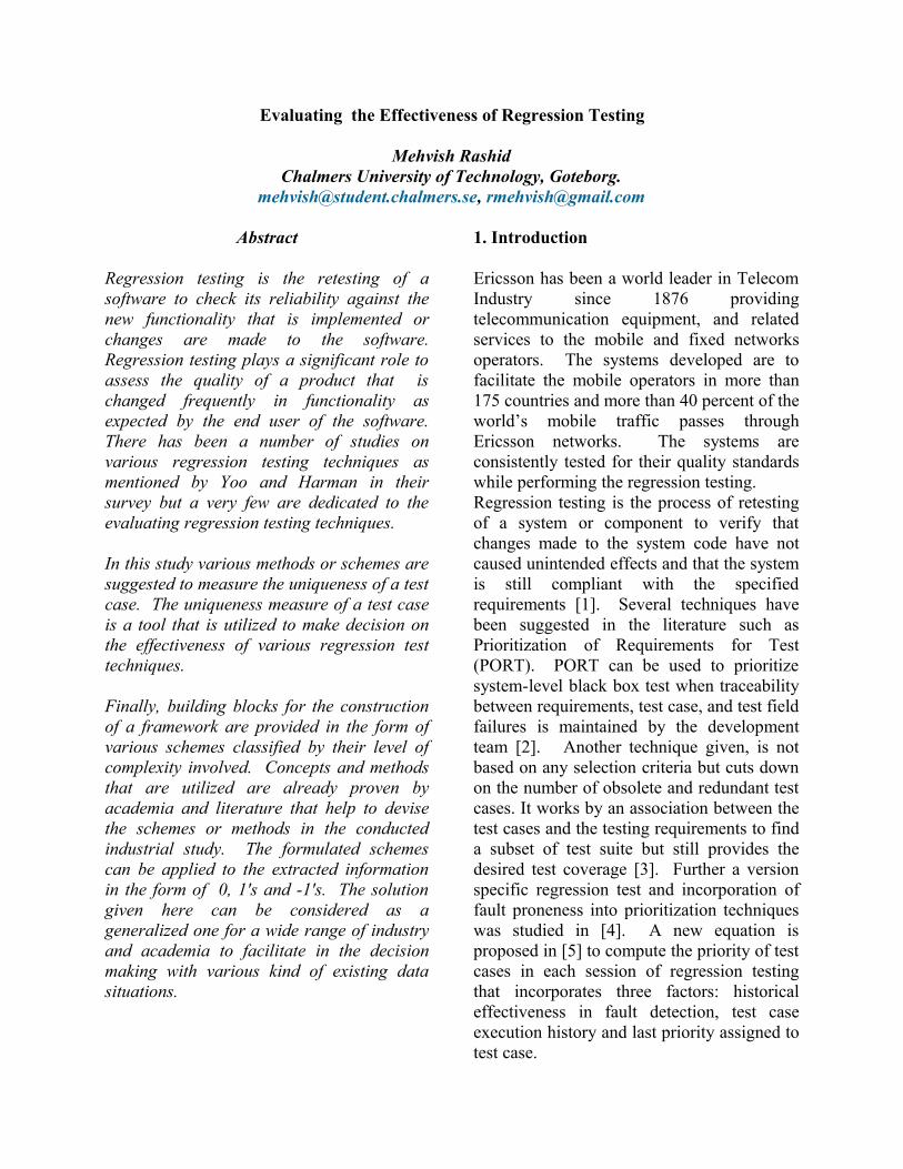
The similarity behavior of subset of test cases can be predicted by comparing the probability of pass and fail from the cells A and D in pair wise matrix. The dissimilarity behavior of test case can be identified by comparing the values in the cell B and C. Similarly the value in cell D depicts the behavior of test case in a subset that fail together. This can be a representation of Co-Fail behavior of the test cases in a subset. How often each test case behaves differently from the other test case within the same system is predicted in the outcome in the form of pass and fail. If two test case test the same functionality in a system they are expected to pass or fail together, the only situation one passes and other fails is when they are testing different functionality. Figure 4 represents the behavior of test cases in a test pool with A, B and C different types of functionality in the system. Test case 2, 3 and 4 test the same functionality so it is believed that they pass and fail together.

Figure 4: A, B and C three areas of test subject. tc1, tc2 and tc3 test the same area

Understanding the behavior of the test cases in subsets of two test cases with all possible combinations and repeating the process for all selected test runs can give an insight into the test case behavior.

In Figure 5 each cell of the matrix is populated with a value that describes the behavior of the pairwise comparison. The value of the similar behavior can be represented by 1 and dissimilar behavior by -1. Here the idea is to evaluate the two test cases based on their behavior when they are executed together in a test run. The number of test runs for which test cases are run is denoted by N. For each N number of test run n x n matrix is calculated for n number of test cases. The populated values in the upper half of the triangle and the lower half of the triangle will be same (separated by the highlighted diagonal). Therefore comparison of subsets performed in a n x n matrix for the possible combinations for one diagonal is given by,

Where n is the number of test cases.

5.2 Derivation of Schemes

The four box matrix described in Figure 3 is redrawn in Figure 6 by replacing pass and fail by 1 and -1 respectively. The value 1 is assigned to the cell A that indicates the scenario where both test cases are passing.

Figure 5: The structure of matrix for test case pair-wise comparison for similar/ dissimilar behavior for one test run.

5.2 Derivation of Schemes

The four box matrix described in Figure 3 is redrawn in Figure 6 by replacing pass and fail by 1 and -1 respectively. The value 1 is assigned to the cell A that indicates the scenario where both test cases are passing. The values in the other cells B,C and D are marked by -1. Analyzing Figure 6 three out of all possible combinations are identified in which test case behavior is measured. Each combination of cells is referred to as Scheme. There are three schemes as highlighted in Figure 6 that are used to perform calculations on test case data.

Figure 6: Test case i and j in a pair wise matrix each with pass denoted by 1 and fail by -1 and possible combinations of schemes derivation.

Dissimilar: The scheme is called Dissimilar, since the subset of test cases is analyzed for dissimilar behavior across N sessions. Each cell of matrix is marked by 1 if both test cases have same value or by -1 if they have dissimilar values Figure 7.

Ti,j 1 -1

1 1A

-1B

-1 -1C

1D

Figure 7: Dissimilar Scheme: Test case i and j in a pair wise matrix each subset with same values of test cases are denoted by 1 and dissimilar by -1.

Dissimilar scheme is defined by the value of test case subset by the following:

Rule:If value of two test case is in disagreement i.e. -1 and 1 mark -1- '-1' Here means reverse behaviorIf value of two test case is in agreement i.e. 1 and 1 mark 1- '1' Here means similar behavior

Similar: Similar scheme is the inverse of dissimilar so if the total value for dissimilar is subtracted from 1, result is for the similar scheme as depicted in Figure 8.

Ti,j 1 -1

1 -1A

1B

-1 1C

-1D

Figure 8: Similar Scheme: Test case i and j in a pair wise matrix each subset with same values of test cases are denoted by -1 and dissimilar by 1.

Rule:If value of two test case is in agreement i.e. 1 and 1 mark -1-1 Here means similar behaviorIf value of two test case in disagreement i.e. -1 and 1 mark 11 Here means dissimilar Behavior

Co-Fail: The Scheme highlights the behavior of test cases in a subset that fail together. Figure 9 depicts the values in the cell A,B, C and D of matrix, where -1 in D indicates that both test case fail together.

Rule:If value of two test case is in Agreement i.e. 1 and 1 mark 1If value of two test case in disagreement i.e. -1 and 1 mark 1If value of two test case in disagreement i.e. -1 and -1 mark -1- Here '-1' is the Co-Fail behavior of test cases.

Ti,j 1 -1

1 1A

1B

-1 1C

-1D

Figure 9: Co-Fail Scheme: Test case i and j in a pair wise matrix each subset with same values of test cases are denoted by 1, dissimilar by 1 and Co-Fail by -1.

In order to understand the behavior of the subset in the matrix the cell value of each combination is compared across all selected test runs (sessions) for the times it appears as -1. The percentage of count of behavior (-1) for a single subset across N session is calculated by the following:

In the Figure 5 the vertical column highlighted by a lighter color represents the column vector for the test case in the matrix. The value of dissimilar behavior that is calculated for each subset using the equation above can be added in the order of subsets presented in the column vector for each test case. The sum of the values of subsets in the order of column vector and further calculating the percentage of dissimilar behavior gives the uniqueness value of the test case.

Here i is the number of subsets in the vector for a test case and n is the number of session.

5.3 Pre-processing

The schemes devised in the last section only incorporate data in the form of 1 and -1. In the data presented, 0 indicates missing information as discussed earlier in section 3. However the presence of missing information in the form of 0’s has to be handled to add value to the final calculations. The schemes presented so far do not deal with the missing information. Missing information cannot be ignored since it is important form of information. Section 3.1 gives the reason for the missing information. There can be three alternatives to the missing information.

1. Non-faulty: Consider the reason for missing information for a test case as a non- failure. For instance “Non-faulty” variation is more valid for a situation where a break occurred in the

normal execution of regression test due to the instability of the environment.

2. Most-recent-info: Missing information for a test case can be replaced with the value (pass or fail) for most recent run before the information appeared as a zero. For Instance if there is a newly added test case against functionality.

3. Failure-frequency: For the missing information a value is assigned by calculating the frequency of failures given by the average of total passes and fails. The “Failure Frequency” is given by frequency formula:

The process of transforming the missing information to a more suitable form of information is called Pre-Processing. It is a Pre-Requisite for applying the above suggested schemes containing 0 as missing information.

Dynamic Scheme: Failure frequency given as a third alternative for handling the missing information results in data not in the form of 0’s and 1’s. The data consists of values other than 1 and -1 i.e. 0.7, 0.8,-0.33. The simple comparison of -1 and 1 is not possible now. To measure the uniqueness of a data with varying frequencies another method is required that can facilitate the calculations. Since for each subset of test cases we have two variables in the form Tci and Tcj. The method that is suitable to perform calculations on such variant data is Spearman correlation coefficient. Spearman correlation coefficient makes no assumptions on the distribution of data and therefore can be used here to calculate uniqueness of test cases with

different frequencies. The method is purely statistical and already present to be used for calculations. There are few steps to the formula:

- Rank the data for two variable- Calculate the distance of a subset- Take the square of the distance- Apply the following formula

The formula above gives the value of a subset (i,j), the average of vector for each test case is calculated similar to other schemes.Spearman Correlation coefficient is only applied on data that results from the application of failure frequency alternative for pre-processing. Since the value of frequencies calculated varies due to changing status of test cases in test runs the scheme is referred to as “Dynamic” form of uniqueness.

Average Fault Detection Reduction (AFDR):

Average Fault Detection Reduction (AFDR) is different from the other schemes since no pair wise comparison of test cases or pre-processing step is required and can be applied on any kind of data. The uniqueness of a test case is measured by taking the percentage of a test case failure 'a' across N sessions. Therefore it is denoted by,

The scheme assumes the priori knowledge of the defects from a test run [6] and evaluates regression testing techniques on the basis of finding the maximum number of faults. AFDR is evaluated on the basis of detected

faults in a test suite found by a technique across the n number of test runs. The technique that has a higher average value across all sessions is prioritized. AFDR is given by,

n here is the number of sessions for which the regression test technique is evaluated using AFDR.

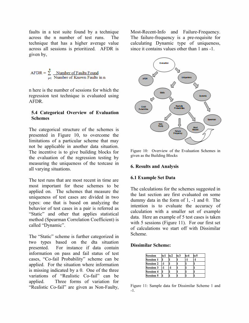
5.4 Categorical Overview of Evaluation Schemes

The categorical structure of the schemes is presented in Figure 10, to overcome the limitations of a particular scheme that may not be applicable in another data situation. The incentive is to give building blocks for the evaluation of the regression testing by measuring the uniqueness of the testcase in all varying situations.

The test runs that are most recent in time are most important for these schemes to be applied on. The schemes that measure the uniqueness of test cases are divided in two types: one that is based on analyzing the behavior of test cases in a pair is referred as “Static” and other that applies statistical method (Spearman Correlation Coefficient) is called “Dynamic”.

The “Static” scheme is further categorized in two types based on the dta situation presented. For instance if data contain information on pass and fail status of test cases, “Co-fail Probability” scheme can be applied. For the situation where information is missing indicated by a 0. One of the three variations of “Realistic Co-fail” can be applied. Three forms of variation for “Realistic Co-fail” are given as Non-Faulty,

Most-Recent-Info and Failure-Frequency. The failure-frequency is a pre-requisite for calculating Dynamic type of uniqueness, since it contains values other than 1 ans -1.

Figure 10: Overview of the Evaluation Schemes in given as the Building Blocks

6. Results and Analysis

6.1 Example Set Data

The calculations for the schemes suggested in the last section are first evaluated on some dummy data in the form of 1, -1 and 0. The intention is to evaluate the accuracy of calculation with a smaller set of example data. Here an example of 5 test cases is taken with 5 sessions (Figure 11). For our first set of calculations we start off with Dissimilar Scheme.

Dissimilar Scheme:

Session tc1 tc2 tc3 tc4 tc5Session 1 1 1 1 -1 -1Session 2 -1 1 1 1 1Session 3 -1 -1 1 1 1Session 4 1 1 1 1 1Session 5 1 1 1 1 1

Figure 11: Sample data for Dissimilar Scheme 1 and -1.

The first step is to make combinations by using the formula below:

Comparison step is followed by the comparison of test cases with in each subset resulting from the combination. Column S1, S2 to S5 show the number of sessions that each subset is compared for, which in itself is a two dimensional matrix. The test cases having reverse behavior are marked by -1 and with similar behavior as 1 in Figure 12. The percentage of dissimilar behavior is calculated across all (five sessions).

Comp S 1 S 2 S 3 S 4 S 5 %1,2 1 -1 1 1 1 0,21,3 1 -1 -1 1 1 0,41,4 -1 -1 -1 1 1 0,61,5 -1 -1 -1 1 1 0,62,3 1 1 -1 1 1 0,22,4 -1 1 -1 1 1 0,42,5 -1 1 -1 1 1 0,43,4 -1 1 1 1 1 0,23,5 -1 1 1 1 1 0,24,5 1 1 1 1 1 0

Figure 12: Comparison of n x n matrix populating each cell with its pair-wise dissimilar behavior.

Finally the uniqueness of each test case is calculated by taking the average of the column vector for each test case as shown in Figure 13.

Figure 13: Taking the average of Column Vector of test cases to give measure of uniqueness.

The uniqueness measure calculated in Figure 13 shows that test case 3 is most unique and test case 1 is least unique. If we compare the values of uniqueness with the example data in Figure 11, the results of uniqueness are in accordance to it since the dissimilar behavior of test case 1 is evident in Figure 11. Test case 3 does not display any dissimilar behavior still a uniqueness measure is given by a value of 0.0020. The value of uniqueness measure is calculated on the basis of test cases interaction in test pool with other test cases. Test case 3 displays dissimilar value when uniqueness measure is calculated, that is there due to its interaction with other test cases in the form of column vector. Taking the average value of column vector against a test case incorporates the interaction of test cases in the test pool. Co-Fail Scheme

Co-Fail Scheme percentage calculations for dissimilar behavior are shown in Figure 14. Test case 1, 2, 4, and five Co-Fail with each other as seen in the Example data. The calculated value for uniqueness measure (Figure 15) after taking the average of vector for each test case verifies the situation in the example data. Test case 3 does not co-fail with any of the other test cases therefore the value for uniqueness measure is 0.

Combination S1 S2 S3 S4 S5 %1,2 1 1 -1 1 1 0,21,3 1 1 1 1 1 0,41,4 1 1 1 1 1 0,61,5 1 1 1 1 1 0,62,3 1 1 1 1 1 0,22,4 1 1 1 1 1 0,42,5 1 1 1 1 1 0,43,4 1 1 1 1 1 0,23,5 1 1 1 1 1 0,24,5 -1 1 1 1 1 0

Figure 14: Percentage of Co-Fail behavior for each pair of comparison.

Testcase 1

Testcase 2

Testcase 3

Testcase 4

Testcase 5

1,2 1,2 1,3 1,4 1,5

1,3 2,3 2,3 2,4 2,5

1,4 2,4 3,4 3,4 3,5

1,5 2,5 3,5 4,5 4,5

Uniqueness 0,25 0,25 0 0,25 0,25

Figure 15: Uniqueness Measure for Co-Fail for test case 1, 2, 4 and 5.

Pre-processing Calculations

0 with 1 (Non- Faulty)

The data where information is missing by the indication of 0 (Figure 16), a pre-processing step (discussed in section 5.3) is performed shown in Figure 17 to replace 0 with 1 (Non-Faulty). Further calculations can be done by measuring uniqueness with dissimilar behavior or Co-fail behavior (Figure 18 in Appendix 3 ) and Figure 19.

Figure 16: 0’s in the Example Data Set

Figure 17: 0’s replaced with 1’s in the Example Data Set

Figure 19: Uniqueness Measure of Dissimilar Behavior in Non-Faulty.

0 with -1 (Most-Recent-Info)

In this example the 0’s are replaced with -1 or 1 whichever is the status of test case in the most recent test run similar to as shown in Figure 17. The calculations are performed similar to using dissimilar behavior as shown in Figure 18 (Appendix 3) and 19.

Failure Frequency with Dynamic Spear man Co-relation Coefficient

The third form of handling missing information proposed in this study is the average of pass and fail status of test cases using frequency formula given in section 5.3 and replace 0 with that number. As shown in Figure 20 (appendix 3), the failure frequency is calculated for test case 1 (column tc 1) for sessions 6 and 7 with resulting value -0.2. The frequency is again updated for sessions 9 and 10 since another 1 appears in session 8. The data is now in the form of fractional or decimal numbers. Dynamic Scheme is used here to perform calculations to find the uniqueness of test cases. The calculations are based on three steps of spearman correlation coefficient such as ranking, distance, Square of distance and finally the application of formula (Figure 22 Appendix 3). After the value of Rho is known for a subset of test cases in comparison within n sessions, the average of vector value is calculated for each test case (Figure 23).

Figure 23: Calculation for Uniqueness Measure for Dynamic Scheme

AFDR

Average Fault Detection Reduction (AFDR) requires less computation as compared to other schemes presented so far. The Uniqueness is measured by taking the average of test case failure across n number of sessions (Figure 24).

Sessions tc1 tc2 tc3 tc4 Tc5Session 1 1 1 1 -1 -1Session 2 -1 1 1 1 1Session 3 -1 1 1 1 1Session 4 -1 1 1 1 1Session 5 1 1 -1 -1 1Session 6 1 -1 -1 1 1Session 7 -1 -1 -1 1 1Session 8 1 1 -1 1 1Session 9 1 -1 1 1 1Session 10 1 1 -1 1 1a/NUniqueness 0,4 0,3 0,5 0,2 0,1

Figure 24: Calculation for Uniqueness Measure in AFDR for individual Test cases.

For each session selected regression testing techniques are evaluated by the number of known faults it finds. The average of uniqueness measure is taken for all test cases detected as faults by the selected techniques for n sessions. The final results are shown in Figure 25 in Appendix 3.

Weighting Schemes with AFDR

Time is an important factor since the information of a test run is directly related to the specific instance of time it was executed

during a product development. The test runs back in time are not that valuable as the recent ones. Recent test runs give the current status of a defects found in software. The information found for defects relating to farther back in time is not as valuable. To incorporate the details of time factor weighting schemes are multiplied with the AFDR values. Calculation for two weighting schemes: Exponential Moving Average (EMA) and Modified Moving Average (MMA) are given in Figure 27 and 28 (details Appendix 2). It appears from Figure 28 that MMA gives better results in comparison to Figure 26 when the recent test runs are prioritized in time.

Figure 26: Graph of AFDR with Technique A and Technique B.

Figure 27: Graph of AFDR with Technique A and Technique B using EMA.

Figure 28: Graph of AFDR with Technique A and Technique B using MMA .

6.2 Choice of Scheme for Finding Uniqueness

The calculations performed so far by applying different schemes based on varying situation of data facilitates to refine the abstract categorical classification in Figure 10 into a more detailed one given in Figure 29. AFDR appears on the top since it can be performed on any kind of data. In case the information is not missing and intention is to do pair wise comparison for finding uniqueness, the choice can be either co fail or dissimilar scheme. Conversely for missing information one of pre-processing step is performed. pre-processing based on failure frequency that results into decimal data, uniqueness of test case is calculated by applying dynamic scheme. pre-processing step based on non-failure or most-recent-info gives the choice of either applying co-fail or dissimilar behavior. Similar scheme can be applied as well but not shown in this study since it is reverse of dissimilar. Collectively (excluding similar) eight different schemes can be derived by following the decision tree as shown in Figure 29.

6.3 Empirical Evaluation

In section 6.2 based on Figure 29 eight schemes for calculating the uniqueness

measure are highlighted. Two main telecommunication projects A and B are selected to evaluate the suggested schemes in section 3.3 on the previous regression test executions. The overall estimated size of product A and B is about 1,250 and 110 thousands Line of Code.

Figure 29: Choice of Scheme for Calculating Uniqueness Measure (enlarged Appendix 3)

As explained in section 3 of Appendix 2, a product is constituted from projects developed in version branches. To evaluate the schemes suggested in the preceding section two version branches were selected within two products. Each branch's development progress varies with time as shown in Figure 30 below.

In order to analyze the behavior of test cases if we consider them in multiple version branches then the results will not be valid since each of the branch progress is different in time as is the nature of implemented functionality. Here the branch versions

selected for the empirical evaluations are referred as A1 and B1.

Out of most recent test runs 50 are selected for A1 and A2 with 25 test cases to perform the calculations. Evaluation of eight schemes on two different regression test techniques with most recent test runs of 20, 25 and 50 are shown in the Figure 31 (Appendix 3).

Figure 30: Comparison of Progress of version branches at an instance. Each branch progress varies with time

Since the main aim of this study is not concerned with the design of regression test selection techniques, two test suites are selected based on even and odd number of test cases and then taking the average of their uniqueness measure. The test suites are referred as TA and TB for even and odd respectively.

The value of uniqueness measure is observed to vary with the number of sessions. Overall the value of uniqueness measure depends upon the existing behavior measured across n sessions. For instance scheme 4 in Figure 31 (Appendix 3) dissimilar 0 to latest uniqueness measure decreases with added number of test runs. In case of Spearman the value of uniqueness increases comparatively in 50 sessions than in 25 sessions. Uniqueness Measure varies with the data representation in the across test runs and the extent to which behavior is quantified in computations.

For the TA and TB evaluated with eight different schemes the technique that gives the

higher value of uniqueness measure is valued the most.

7. Discussion

In Figure 31 (Appendix 3) calculations are performed on eight schemes with different data situations. The first situation of data is without missing information given by 1 and 2 under schemes in Figure 31. The value of dissimilar behavior is higher than Co fail behavior. The values from calculation may vary and much dependent upon the representation of specific behavior of the data used. For instance, if the data had higher display of co-fail behavior than dissimilar behavior the results would have been different. From Scheme 3 to 6 the calculations are performed using the pre-processing step. Pre-processing by non-failure (replacing by 1) does not give high value for dissimilar and co fail behavior. On the other hand most recent info pre-processing where the test case is considered to fail in most recent test run effects the calculations in Scheme 4 and 6. In Scheme 7 and 8 two different ways of computations are employed one is by applying spearman correlation and other by comparing the number of faults found.

In all eight schemes the calculations were performed with 20, 25 and 50 test runs. At times with increased number of test runs the computations gave lower value of uniqueness for test cases and therefore the resulting test suite. In case of Scheme 8 the uniqueness value seems to get better with the increasing number of test runs but this is also dependent on variation in data. Therefore, for the evaluation of regression technique an average of calculations with varying numbers of test runs can be considered as in column “Average TA” and “Average TB” in Figure 31 (Appendix 3).

The variation in data and difference in the mechanism of test suite selection by employing diverse regression test techniques does not provide a generalize way of knowing which schemes always gives better result for a particular regression test technique. Experimentation and evaluation of specific regression test techniques is required with the presented schemes to establish that a specific technique gives better evaluation with a particular regression test technique.

The application of the schemes devised is more about providing different methods to measure the uniqueness of a test case with varying situations of data. Situation depends on the kind of events that occur during the execution of regression test i.e. break in the execution session or skipping a particular test case for execution. In order to weight the significance of a single test case all factors affecting its value are considered. In this study the quality attributes of the test cases are not mapped at test case level therefore the computations for finding the uniqueness of a test case are solely based on the calculations presented by different schemes. The schemes or methods for calculation can act as the building blocks for the construction of a framework that provide a uniqueness measure for test cases with various form of information presented from executions of test runs.

Uniqueness measure of a test case is the measurement instrument for finding whether a test case should be included in a test suite for regression test or not. In a test pool of test cases uniqueness measure can serve as an indication of behavior for grouping them together. Once the uniqueness measure of each test case is known it is easier to segregate effective regression testing techniques that select test cases with similar behavior. Here since the details of the quality attributes were not incorporated at test

case level the evaluation of regression testing technique is simply by taking the average of the uniqueness measure of test cases in test suite. Even after the incorporation of quality attributes the main calculations for measuring uniqueness of a test case would remain same as presented in the given schemes. Quality attribute information can be introduced as a pre-processing step linked through the database containing information on each test case or can be linked to the final value of uniqueness measure found by applying a scheme. The linking of quality attributes to a test case can be a candidate topic for future study.

Statistical method adopted for calculations are already present in academia and literature. For instance, spearman correlation is used to find the relation between two variables. Since the comparison of test cases is in pairs we get two different variables to perform calculations on. Also different number of test runs constitutes multiple row data for each set of variable and finally a single value for correlation is given. The method suffices the goal of finding uniqueness for data with fractional values or other than 1 and -1. Time is an important factor when regression testing is conducted. The defects resultant of change in the software gives the current status of software functionality. The number of defects found in the recent time is important than the previous ones. Therefore the test runs from the most recent regression runs are more valued since they give the developers and testers the insight into the further efforts required for an acceptable quality standardized software. In the Schemes presented the data is selected from the most recent regression test runs and then a value for uniqueness measure is calculated across test runs. Time based information gives updated calculations so that if a test case becomes less important with time the details are incorporated in the calculations.

In the schemes presented so far the least efforts and resources are involved in performing calculations using Average Fault Detection Reduction (AFDR). AFDR is the simplest kind of calculations than the pair-wise comparison and can be performed easily in all varying situations of data. This is why AFDR is kept in a separate branch in the categorical classification of uniqueness measure schemes. Main ideas from the discussion are summarized below:

Handling Different Situations with Data without Generalization: Different Regression test selection techniques may give different results with the presented schemes.Framework: The Schemes can be used as the building blocks for finding the uniqueness of test cases in different situations of data.Measurement Instrument: Finding the uniqueness of a test case in the test pool is the main tool to measure a test case.

Adoption of Statistical Methods: Methods applied for calculation already exist and are used with variation according to the current need in the organization

Time Variance: Calculations are dynamic that incorporate the details of changing state of software development with time, i.e. more failure when application is under development.

8. Conclusion

Uniqueness for a test case is a measure of its relation or association with other test cases in the test pool. Once this uniqueness measure is established it ha been utilized to evaluate the test suite found by a specific regression technique. In this study an overview of different schemes is given that can be used for the evaluation of regression testing. The two main categories of uniqueness are identified as static co-fail and realistic co-fail. In static co-fail the missing information for test cases in the form of 0 is not handled and therefore a variation of realistic co-fail is applied. Finally a scheme is given AFDR that does not measure the uniqueness of test cases but evaluates the two regression testing techniques on the average percentage of defects found. Some weighting schemes applied give a better view of the defects found while prioritizing the most recent test run in time than the old one.

The schemes suggested in this study can be used as the building blocks for the evaluation of regression testing techniques. The study is evaluated empirically on the real situation in software industry and therefore can be considered as a potential candidate for the implementation on large sized industry projects in the future.

References

[1] IEEE, “IEEE Standard 610.12-1990, IEEE Standard Glossary of Software Engineering Terminology,” 1990.

[2] Srikanth, H. Williams, L. Osborne, J. “System test case prioritization of new and regression test cases”, Empirical Software Engineering, page 10, 2005.

[3] Harrold, M.J., Gupta, R., Soffa, M.L., “A methodology for controlling the size of a test suite, ”Software Maintenance, 1990., Proceedings., pages 302 – 310, 2002.

[4] Elbaum, S., Malishevsky, A.G., Rothermel, G., “Test case prioritization: a family of empirical studies”, Software Engineering, IEEE Transactions, pages 158-182, 2002.

[5] Fazlalizadeh, Y.; Khalilian, A.; Azgomi, M.A.; Parsa, S., “Prioritizing test cases for resource constraint environments using historical test case performance data”, pages 190- 195, 2009.

[6] Yoo S., Harman M., “Regression Testing Minimization, Selection and Prioritization: A Survey”, Software Testing, Verification and Reliability, John Wiley & Sons, Ltd., 2010.

[7] Mark Sherriff, Mike Lake, and Laurie Williams. “ Prioritization of Regression Tests using Singular Value Decomposition with Empirical Change Records”. In Proceedings of the The 18th IEEE International Symposium on Software Reliability (ISSRE '07). IEEE Computer Society, Washington, DC, USA, 2007, pp 81-90.

Appendix 1: Regression Testing Process and Data

1. Overview of the Testing Process

Testing is conducted in three forms:

Smoke: It is performed first by developers and then by testers. The testers write the test case against the code to test it. Few of the selected test cases are run in smoke and then all the written test cases are added to Regression base test pool.

Daily: Only applies to one product.

Weekly: All test cases are run at the weekend with the jobs scheduled in the form of ready files that contains a selection of the number of test cases. The ready files are executable to be run on scheduler used for the organization.

Defect Fix and Rechecking

TR: A Trouble Report (TR) is written based on PMR (Customer Requirements), defect from the testers or any found defect that results in the TR writing. TR is sent to development team, who after reproducing the defect resolve the problem. The defect is then fixed and is tagged with some defined labels to identify the reason at developments end. Pictorial depiction of Latest Software Version (LSV) cycle just few weeks before the product is shipped to the customer is given below.

Test case: Test case are written against the code developed by the developers

Test Groups: Test cases are grouped into test objects according to main functionality to cover as many positive and negative testing scenarios.

Test execution session / test run: Each test run is maintained in a dedicated session and is stored in MySql Database.

Pass/ Fail: Each test case is assigned pass (indicated by green) and fail (indicated by red)

Outcome of running test runs: The Test cases that fail are assigned a Priority level A, B, C. The stability of a node can be seen by the test runs based on the failed test cases. Failing test case could be because of environment factor or some crucial product defect. Test case failing does not say anything about the quality of the defect. From the organization point of view all failed test case are important because they have potential to find a defect.

2. Database Structure

There are various tables in the database used to store the information on the test runs. The most important tables are Test Groups, Test Runs and StreamSession. The main fields of tables are described below in table 1, 2 and 3.

The test cases are grouped in testobject. Each testobject contains various number of test cases testing the functionality of a feature. It may constitute upon multiple features in a module. These testobjects are contained in a ready file scheduled to be run on automatic Scheduler for the regression test.

TestGroups table contains test object specific details such as unique id, and test object. Two different test cases can be given the same number two different test objects. For instance test case 5 in testobject 1 and testobject 2 indicate different test cases. Therefore, a unique test case is identified with a combination of test object, test case number and a test case slogan.

StreamSessions maintains the details on the session that are run as a part of testing activities. The information of most interest to us is the pass and fail status of the test cases. The pass and fail information in the streamline table is saved in the form of 0’s and 1’s. To retrieve the status of the test cases for a specific number of runs the database can be queried with SQL.

TestRuns gives an overview on the runs of the testing activities. The details are maintained under a session Id with a count of test cases passed and failed.

TestGroups

Field Description

toSeqNr autoincremented unique id for a testobject record

testobject testobject name, used in the streamline table (and others as well)

isRemoved true if testobject is 'deleted' (test objects are never deleted just hidden)

TestRuns table:

Field Description

ruSeqNr auto_increment | autoincremented unique id

Project project identifier, e.g. Project A,B.

dr drop identifier, e.g. daily/weekly

Pass number of passed testcases for this session

fail |number of failed testcases for this session

Nap number of nap testcases for this session

Running true if the session is still running

sessionId session id for the whole testcase execution

StreamSession

Code maintenance for versioning at the Development:

Development approach that is followed is agile. Code is always changing; change mechanism is detected and maintained using ClearCase IBM tool. The subversions trace back to the main delivery branch and give an overview of the progress of application development. TRs written by the testers against a defect are not mapped with the testcases. The information is not stored in the database where one can find TR and related test case against it. There is a missing link in ClearCase tool when it comes to the mapping of test cases and TRs written against them.

Field Description

tcSeqNr auto_increment | autoincremented unique id

tcNumber test case number, unique in combination with testgroups

tcSlogan test case slogan, as displayed on the testing website

tcTimestamp testcase execution timestamp

Project project identifier, e.g. Project A, B.

dr drop identifier, e.g. daily/weekly

testgroup test object name As seen on testing website

tcStatus status, e.g. pass, fail or nap (not applicable)

nap Not Applicable

tcSessionId session id for the whole testcase execution (all testcases in all testobjects)

tcFailCount number of times a testcase have failed in a row

tcRunNumber for testcase history, the highest number is the latest version of the testcase

tcDeleted Is the test case deleted? (we never really delete anything, just hide by using this flag)

tcIsLatestRun True if this row holds the results from the latest testcase execution

errorCategory The error category

assignedTo The team assignment

ClearCase keeps the information on the TR written against code but within the database there is no link between the test cases and the run for specific TR.

Cost of getting other information:

A dummy mapping can be done by tagging TR with test cases in Database to find effective test suite while comparing different techniques for finding a test suite for regression testing. One field can be added to the table containing test cases to tag relevant TR against them. It can useful for decreasing the number of test cases for regression testing in the resultant test suite.

3. Setting Filter for information Retrieval

Within the product there are different projects. The data that is retrieved is from weekly Regression runs. Since there are multiple branch projects within a product, data from a project with in the same version branch is considered for consistency reasons. Since the changes implemented in each branch can vary in functionality, data combination from across all branches will make it inconsistent. As shown in Figure 1 if data for test cases is considered across the branches it would not be appropriate since we want to study the pass and fail behavior of test cases all together. For instance to analyze the behavior of test cases if we consider them across branches then the results will not be valid since each of the branch progress is different in time as is the nature of implemented functionality.

Figure 1: Comparison of Progress of version branches at an instance. Each branch progress varies with time

Product A

Version Branches

Progress at one instance on time line

Appendix 2: Average Fault Detection Reduction and Weighting Schemes

Fault Detection Reduction

1. Calculate the Uniqueness of each test case across n sessions by counting the number of failures. a/n

2. Select two different sets of test cases as a result of Technique X. 3. For each session in the original data see how many faults are present.4. Assumption that each session i contain unique set of faults. Divide the total number of

Faults found by Technique (A) in session i with the total number of faults in session i. The result is FDR(A) and FDR(B).

5. Repeat step 6 for n number of sessions and for each Technique X1 and X2.6. Find the Average of FDR(A) and FDR(B).

Applying Weights

The information from the recent session is the most important. We assign weighting by time. Simplest weighting linear can be used. By looking at the number of sessions spread out the weights so that the later weight are higher and they all sum to 1.

Exponential Moving Average = S t = α * yt +(1-α) *S t-1

Where S t is the MVA for current observation, α is the coefficient value calculated as α= 1/ (N), N is the number of current session,yt is the value of the observation (here FDR),S t-1 is the MVA for last observation.

Modified Moving AverageAnother weighting scheme Modified Moving Average (MMA) that is applied gives a better overview of the trend of uniqueness measure according to the value in time as given below:

α= 1/(N)

Where α is the value of the coefficient applied and N the number of the current session.

Applying Severity

Multiply FDR in session i with the sum of the severities in found faults.Rate the higher severity with higher integer value.

Faults found *Sum of severities of faults found / sum of total faults found.

Adding Cost

Cost can be added if the time for running a test case is known. Then for selected test suite by a technique we can say that we have time to run this many test cases. i.e. a technique selects 80% but due to time limit can only run 40 test cases.

- Data does not have variability, most of the data have similar pattern. Fault Detection Reduction assumes that all faults in each session are unique. By identifying the number of faults found by each technique during each session and taking an average over all sessions we can compare two techniques. Fault Detection Reduction (FDR) is similar to Average Percentage of Fault Detection (APFD) but in APFD the prior knowledge about the number of faults is known.

Appendix 3: Figures

Figure 18: Percentage of Dissimilar Behavior for Non-Faulty

Figure 20: Calculation for Failure-Frequency

Figure 22: Calculation for Distance, Distance Square and Rho for each Pair-Wise Comparison.

Figure 25: Calculation of AFDR on two techniques with Weighting Schemes EMA and MMA.

Figure 29: Choice of Scheme for Calculating Uniqueness Measure

Figure 31: Empirical Evaluation of Eight Schemes with two test suites TA and TB

S c h e m e s T e c h n i q u e A T e c h n i q u e B A v e r g a g e T A A v e r g a g e T B

5

2 0 S e s s i o n s 0 . 0 0 0 2 2 0 . 0 0 0 2 4 0 . 0 0 0 2 8 0 . 0 0 0 3 0

0 . 0 0 0 3 6 0 . 0 0 0 3 8

5 0 S e s s i o n s 0 . 0 0 0 2 7 0 . 0 0 0 2 9

2 C o - F a i l 6

0 . 0 0 0 0 4 0 . 0 0 0 0 3 0 . 0 0 0 2 2 0 . 0 0 0 2 3

2 5 S e s s i o n 0 . 0 0 0 3 5 0 . 0 0 0 3 8

5 0 S e s s i o n 0 . 0 0 0 2 7 0 . 0 0 0 2 8

3 . D i s s i m i l a r ( 0 t o 1 ) 7

2 0 S e s s i o n s 0 . 0 0 0 0 0 0 . 0 0 0 0 0 0 . 0 0 0 1 0 0 . 0 0 0 1 1

2 5 S e s s i o n s 0 . 0 0 0 1 4 0 . 0 0 0 1 5

5 0 S e s s i o n s 0 . 0 0 0 1 6 0 . 0 0 0 1 7

4 . D i s s i m i l a r ( 0 t o l a t e s t ) 3

2 0 S e s s i o n s 0 . 0 0 2 6 2 0 . 0 0 2 7 7 0 . 0 0 2 1 1 0 . 0 0 2 2 9

2 5 S e s s i o n s 0 . 0 0 2 0 5 0 . 0 0 2 3 5

5 0 S e s s i o n s 0 . 0 0 1 6 5 0 . 0 0 1 7 5

5 . C o - f a i l ( 0 t o 1 ) 8

2 0 S e s s i o n s 0 . 0 0 0 0 4 0 . 0 0 0 0 3 0 . 0 0 0 0 5 0 . 0 0 0 0 4

2 5 S e s s i o n s 0 . 0 0 0 0 6 0 . 0 0 0 0 5

0 . 0 0 0 0 5 0 . 0 0 0 0 3

6 . C o - f a i l ( 0 t o l a t e s t ) 4

2 0 S e s s i o n s 0 . 0 0 1 1 5 0 . 0 0 1 0 3 0 . 0 0 1 0 3 0 . 0 0 0 9 5

2 5 S e s s i o n s 0 . 0 0 1 2 1 0 . 0 0 1 1 0

5 0 S e s s i o n s 0 . 0 0 0 7 3 0 . 0 0 0 7 1

7 . S p e a r m a n ( F a i l u r e F r e q u e n c y ) 1

2 0 S e s s i o n s 0 . 4 6 6 3 5 0 . 4 8 3 8 2 0 . 4 8 6 1 3 0 . 4 9 1 2 8

2 5 S e s s i o n s 0 . 4 9 4 6 7 0 . 4 9 2 2 7

5 0 S e s s i o n s 0 . 4 9 7 3 6 0 . 4 9 7 7 5

8 . A F D R 2

2 5 S e s s i o n s 0 . 0 7 5 6 0 . 0 8 0 0 0 . 0 7 5 6 0 . 0 8 0 0

1 . D i s s i m i l a r

2 5 S e s s i o n s

2 0 S e s s i o n s

5 0 S e s s i o n