Evaluating the Consumer Response to Fuel Economy: A

Review of the Literature

Gloria Helfand and Ann Wolverton

Working Paper Series

Working Paper # 09-04 August, 2009

U.S. Environmental Protection Agency National Center for Environmental Economics 1200 Pennsylvania Avenue, NW (MC 1809) Washington, DC 20460 http://www.epa.gov/economics

Evaluating the Consumer Response to Fuel Economy: A Review of the Literature

Gloria Helfand and Ann Wolverton

NCEE Working Paper Series Working Paper # 09-04

August, 2009

DISCLAIMER The views expressed in this paper are those of the author(s) and do not necessarily represent those of the U.S. Environmental Protection Agency. In addition, although the research described in this paper may have been funded entirely or in part by the U.S. Environmental Protection Agency, it has not been subjected to the Agency's required peer and policy review. No official Agency endorsement should be inferred.

1

Evaluating the Consumer Response to Fuel Economy: A Review of the Literature

By Gloria Helfand and Ann Wolverton1

U.S Environmental Protection Agency

Abstract

How consumers evaluate trade-offs between the cost of buying additional fuel economy

and the expected fuel savings that result is an important underlying determinant of the

overall cost of national fuel economy standards. Models of vehicle choice are a means to

predict the change in consumers’ vehicle purchase patterns, as well as the effects of these

changes on compliance costs and consumer surplus. This paper surveys the literature on

vehicle choice models and finds a wide range in methods and results. A large puzzle

raised is whether automakers build into their vehicles as much fuel economy as

consumers are willing to purchase. This paper examines possible reasons why there may

be a gap between the amount consumers are willing to pay for fuel economy and the

amount that automakers provide, though there is insufficient evidence on the relative

roles of these various hypotheses. Further research on the role of fuel economy in

consumer vehicle purchases is needed to assist in understanding the welfare effects of

fuel economy regulation.

Key Words: Consumer behavior, vehicle purchase decisions, fuel economy, energy

paradox, vehicle choice

JEL Codes: D11, D12, D22, R41

1 Authors can be contacted via email at helfand.gloria@epa.gov and wolverton.ann@epa.gov. The views expressed in this paper are those of the authors and do not necessarily represent those of the U.S. Environmental Protection Agency. This paper has not been subjected to EPA’s formal review process and therefore does not represent official policy or views. We are very grateful for the suggestions and contributions of Matt Massey, Chris Moore, two anonymous reviewers, and participants at our presentation at the World Congress of Environmental and Resource Economics.

2

1. Introduction

On April 1, 2010, the U.S. Environmental Protection Agency (EPA) and the

Department of Transportation (2010a) issued regulations to reduce greenhouse gas

(GHG) emissions from vehicles and increase the stringency of Corporate Average Fuel

Economy (CAFE) standards.2

In analyses of the potential economic impacts of fuel economy and GHG

standards for cars and trucks, U.S. Federal agencies have commonly assumed that the

market shares of the vehicle fleet stay constant. For rules that lead to small changes in

vehicle attributes and prices, this may not be a bad approximation, since we would not

expect consumers to make large changes in vehicle purchase patterns in response.

Proposals to increase fuel economy substantially, on the other hand, may cause producers

to change both vehicle attributes and the price of vehicles enough that consumers

noticeably alter their decisions about what vehicles to purchase.

A key analytic question that was discussed in the

evaluation of the standards was the role that fuel economy plays in consumers’ vehicle

purchases. Do consumers properly account for the fuel savings from more fuel-efficient

vehicles when making purchase decisions? Will the requirement of additional fuel

economy increase or reduce consumer and producer welfare? This topic is also likely to

be highly relevant in other countries as they contemplate setting or tightening their own

fuel efficiency and/or GHG tailpipe standards. For instance, the International Council on

Clean Transportation (ICCT) finds that a number of countries are contemplating

increasingly stringent mandatory GHG standards for vehicles (ICCT 2010).

2 Because the primary source of GHG emissions from vehicles is burning fuel, reducing fuel consumption will reduce emissions. CAFE standards require the sales-weighted fuel economy of a manufacturer’s fleet to achieve minimum levels.

3

In addition, whether consumers accurately evaluate trade-offs between the costs

of consuming more fuel economy and the expected fuel savings is a matter of some

debate in the literature. Government intervention in markets is commonly justified by the

existence of one or more market failures, such as environmental externalities associated

with a private market transaction or behavior. For instance, vehicle tailpipe emissions

contribute to climate change, an impact not priced into consumer purchase or driving

decisions. If significant numbers of consumers and/or producers also routinely make

mistakes when factoring fuel economy into vehicle purchase decisions, then regulation

may save consumers money in addition to reducing externalities.3

Consumers should be interested in the fuel economy of the vehicles they purchase

apart from what is induced by government regulation: An increase in fuel economy

reduces the private cost of driving. Empirical studies of the effects of higher fuel prices

indicate that higher fuel costs do seem to trigger efforts on the part of consumers to

reduce their gasoline consumption through changes in driving behavior and vehicle

purchase decisions. However, simple present value calculations comparing upfront costs

to future fuel savings indicate that there appear to be many low cost opportunities to

reduce fuel consumption that are not undertaken, even when they could pay off over

relatively short time periods. This observation is commonly termed the “Energy

Paradox.” It is unclear, however, whether such a paradox by itself justifies additional

fuel economy requirements. Some vehicle purchasers may derive pure financial gains

from the additional fuel savings if, for instance, they made mistakes in calculating fuel

savings or relied on rule of thumb calculations at the time of purchase. Other consumers

3 The effect of fuel economy regulations on consumer and producer surplus would need to be combined with these external effects to estimate the total benefits and costs of fuel economy regulation.

4

may be made worse off in their vehicle purchase decision if, for instance, they incur

additional costs for an attribute that they view as uncertain or risky or that they were

unwilling to buy.

This paper reviews the large but inconclusive literature on the role of fuel

economy in consumers’ vehicle purchase decisions. A primary objective of this review is

to highlight key gaps in the existing research that make accurate modeling and

quantification of the welfare effects associated with raising CAFE standards difficult.

Section 2 reviews the state of the art in vehicle choice modeling, with a focus on the role

of fuel economy in these models. Section 3 examines the various explanations posited in

the literature for why consumers appear to undervalue fuel economy. Section 4 discusses

the few studies that focus on the producer side of the equation: why, even if consumers

actually would buy vehicles with greater fuel economy, automakers may not supply

vehicles with the mix of attributes consumers want. Section 5 concludes.

2. State of the Art in Vehicle Choice Modeling

There are a variety of tools available to examine consumers’ valuation of different

vehicle attributes. Hedonic models, for instance, regress vehicle model attributes, such as

fuel economy and horsepower, on the market price of the vehicle to estimate consumers’

implicit willingness-to-pay for each individual feature (e.g., Court 1939, Arguea et al.

1994, Espey and Nair 2005).4

4 Freeman (2003) is a classic reference on nonmarket valuation, including hedonic models.

Because a simple hedonic regression is a reduced-form

equation where market price and quantity are jointly determined by supply and demand,

separately identifying the demand function requires additional modeling. Papers that use

a two-stage approach can examine how changes in external conditions affect demand for

5

a particular attribute. For instance, Ohta and Griliches (1986) examine how changes in

gasoline prices affect the shadow price for particular vehicle characteristics, including

fuel economy, power, and weight. Fan and Rubin (2010) estimate consumers’

willingness-to-pay for fuel economy while accounting for demographic differences such

as age and education. Agarwal and Ratchford (1980) estimate a hedonic price function as

the first step to predicting how consumers would rank order different makes and models.

When evaluating the potential impacts of fuel efficiency or GHG standards, it is

important to understand how changes in stringency could affect the number and types of

vehicles purchased based on their new (post-policy) mix of attributes. Investigating this

empirical question requires the use of models that examine consumers’ choices of

vehicles. For instance, many studies econometrically estimate vehicle choice as a

function of prices, consumer characteristics (such as income, family size, and age), and

vehicle attributes (such as a vehicle’s power and fuel economy). Once estimated, these

models are often used to examine how consumers’ vehicle purchase decisions are

affected by marginal changes in vehicle or personal characteristics. While the focus is on

the consumer in these papers, many also model production decisions in recognition that it

is the interaction between producers and consumers that leads to observed market

outcomes. Other papers evaluate large-scale policy changes by simulating how

consumers and producers in the vehicle market would respond to policies such as an

emissions tax or substantially tighter fuel economy standards. These models often do not

uniquely estimate their own parameters, instead borrowing from the vehicle choice

literature. While we discuss both types of models in this paper, we focus mainly on issues

related to the econometric estimation of vehicle choice models.

6

Reflecting the complexity of consumers’ decisions, models of vehicle choice vary

widely. This section begins with a discussion of the range of research questions explored

by the literature to set the stage for the issues that arise in the models. Next, we discuss

the modeling frameworks that have been developed to examine vehicle choice in the

context of these questions. In particular, we review the modeling approaches, data

sources, and individual buyer and vehicle characteristics included in the models. Vehicle

choice is a rich area of research both because of its direct policy relevance – for instance,

the importance of the auto industry in the U.S. economy, the increasing attention to the

contributions of vehicles to greenhouse gas emissions, and large fluctuations in fuel

prices over time - as well as a multitude of technical challenges. The reader also will note

the large number of working papers referenced throughout the document. Reliance on

only published work for this discussion would neglect a large portion of the literature that

offers innovative new estimation techniques and intriguing results. With or without the

inclusion of these new papers, a review of the literature suggests that the models vary

greatly on a number of dimensions. In particular, and of special interest for policy

analysis, they continue to produce widely varying estimates of the role of fuel economy

in consumers’ purchase decisions.

2a. Research Questions

The auto market has attracted a great deal of research interest because of its size,

its market structure, the availability of data, and its role in a number of significant policy

areas, including international trade and environmental quality. Vehicle choice models

have been developed to analyze many of these research and policy questions. These

models have also served to advance the state of economic modeling: the work of Berry et

7

al. (1995), for instance, is often cited outside the motor vehicle context for its

incorporation of multiple new modeling issues into its framework.5 In the public policy

arena, topics have included the effects of voluntary export restraints on Japanese vehicles

compared to tariffs and quotas (e.g., Goldberg 1995), the market acceptability of

alternative-fuel vehicles (e.g., Brownstone et al. 1996; Brownstone and Train 1999;

Brownstone et al. 2000; Greene 2001; Greene et al. 2004), the effects of introducing and

removing vehicles from markets (e.g., Petrin 2002; Berry et al. 2004), causes of the

decline in market shares of U.S. automakers (e.g., Train and Winston 2007), and the

effects of gasoline taxes (e.g., Austin and Dinan 2005; Bento et al. 2005, Feng et al.

2005), “feebates”6

The research question of interest often affects the structure of the model used to

investigate the choices consumers make in the vehicle market. For instance, some studies

consider only the market shares of new vehicles (e.g., Train and Winston 2007), while

others include the choice between new vehicles and a generic outside good (e.g., Berry et

al. 1995; Klier and Linn 2010a; Whitefoot et al. 2011), and some explicitly consider the

relationship between the new and used vehicle markets (e.g., Bento et al. 2005, 2009;

Busse et al. 2010; Allcott and Wozny 2010). Focusing on market share is sufficient, for

instance, to examine the decline in market shares of domestic U.S. auto producers, but it

would not be appropriate for estimating the effect of a gasoline tax on total vehicle sales.

(e.g., Greene et al. 2005b; Feng et al. 2005; Greene 2009), and fuel

economy standards (e.g., Goldberg 1998; Austin and Dinan 2005; Klier and Linn 2010a,

2010b; Jacobson 2010; Whitefoot et al. 2011).

5 For instance, Bresnahan et al. (1997) apply the Berry et al. approach to analyze personal computer purchases, and Nevo (2001) uses it to evaluate ready-to-eat cereals purchases. 6 A feebate system subsidizes fuel-efficient cars with revenue collected by taxing fuel-inefficient vehicles.

8

Including a generic outside good allows estimation of total market size, but it cannot look

at the effect of changed new vehicle sales on the used vehicle market.

Some studies focus on estimating the role of a specific vehicle attribute in

consumer purchase decisions (e.g., Alcott and Wozny 2010, Busse et al. 2010, Sallee et

al. 2010, Kilian and Sims 2006, Sawhill 2008, Langer and Miller 2011). For instance,

several of these papers examine how vehicle markets adjust in response to changes in

gasoline prices. These studies often rely on panel data approaches and highly

disaggregated data on individual consumer vehicle purchases but do not analyze them in

the context of the alternatives not chosen.

Studies that seek to evaluate a consumer’s choice of a particular vehicle over

other available alternatives often use discrete choice models (e.g., Goldberg 1995, 1998;

Berry et al. 1995, 2004; Train and Winston 2007). These models allow the researcher to

evaluate the relative roles of price, vehicle attributes, and - at times – consumer

characteristics in the vehicle purchase decision. While some discrete choice studies

include only consumer behavior (e.g., Brownstone et al. 1996, 2000; Mohammedian and

Miller 2003; Train and Winston 2007), many jointly estimate demand and supply (Berry

et al. 1995, 2004; Bento et al. 2005, 2009; Whitefoot et al. 2011), and others jointly

model vehicle purchase decisions and vehicle miles traveled (e.g., Goldberg 1998; Bhat

and Sen 2006; Bento et al. 2005, 2009; Feng et al. 2005; Spissu et al. 2009). Empirical

strategies, estimation challenges, and the relative importance of fuel economy in discrete

choice modeling are the main focus of the remainder of Section 2.

As previously mentioned, studies that examine the overall welfare implications of

a new approach or policy (e.g. such as a gasoline tax) often use a market equilibrium

9

model to simulate the effects of the policy on vehicle demand and supply (e.g. Austin and

Dinan 2005; Goldberg 1998; Bento et al. 2005, 2009). These models may involve

original estimation of the demand side, the supply side, or both, or they may be wholly or

partially constructed using parameters borrowed from the literature regarding the

relationship between changes in price and shifts in the demand and supply for different

vehicle attributes.

2b. Empirical Estimation Methods

In models that empirically investigate vehicle purchase behavior, choices are

typically unordered and discrete (e.g., whether to purchase a vehicle; which type of

vehicle to purchase). Underlying the theory of discrete choice modeling is the

assumption that a consumer’s choice will result in higher utility relative to other available

options. Using this theoretic construct, the analyst can build an empirical model that

estimates what factors influence the probability that a consumer will purchase a particular

vehicle. A minor variant estimates the market share for each vehicle type based on

aggregate market data instead of micro-level data. Because market share is based on the

same underlying utility theory, the estimated equations can also be interpreted as

predicting the probability that consumers will purchase a specific vehicle.

The primary methods used in the literature to model discrete vehicle choices,

nested logit and mixed logit, were developed to avoid a pitfall of the simple multinomial

or conditional logit. A simple multinomial logit has the embedded assumption of

“independence of irrelevant alternatives” (IIA): a change in one choice does not affect

the relative preferences for other choices. For instance, under IIA, if the price of a large

truck goes up, the consumer’s preference for switching to another alternative is governed

10

by market shares, not by similarity across vehicles. Thus, the model might predict that

the consumer switches to a mid-size car that sells well instead of to another large truck.

The IIA assumption is generally not considered plausible in the vehicle market.

The nested logit structures consumer choices into “nests” or layers. For instance,

the first layer may be the choice of whether to buy a new vehicle or some other good,

including a used vehicle; given that the person chooses a new vehicle, the second layer

may be whether to buy a car or a truck; given that the person chooses a car, the third layer

may be the choice among an economy, midsize, or luxury car. Within a nest IIA holds,

but the assumption does not apply across nests. In other words, the nested logit accounts

for the fact that some vehicles are closer substitutes than others. If a consumer has sorted

into the midsize nest and the price of her chosen vehicles goes up, she is more likely to

choose another midsize vehicle (which is in the same nest) than an economy car (which is

in a different nest), though her relative preferences among midsize cars remain

unchanged. There is no definitive way to test whether one nesting structure is superior to

another, however, which means that the question of how best to model consumer

decisions may remain unsettled even when alternative nesting structures result in

significant differences in results (Greene 2008).7

7 The sequence of choices made by the consumer at the time of purchase often dictates an intuitive nesting structure (e.g., first a consumer decides whether to buy a vehicle, then what type of vehicle to buy). Some advocate the use of likelihood dominance criterion to choose between models with alternative nesting structures. If the difference between log-likelihood functions is large, then the test allows one to determine the superior nesting structure. If the difference is small, then the test cannot be used to distinguish between two possible nesting structures. See Haab and McConnell (2002) for a more detailed discussion.

It is also important to keep in mind that

the complexity of the model increases rapidly with the number of nests, which can make

it challenging to achieve model convergence to a unique solution. Examples of nested

logit models used to examine vehicle choice decisions include Goldberg (1995, 1998),

11

Mohammadian and Miller (2003), Greene et al. (2005b), Eftec (2008), Gramlich (2010),

Allcott and Wozny (2010), and Klier and Linn (2010a).8

A mixed logit model (also known as a random coefficients logit) relaxes the IIA

assumption by allowing for a more general substitution pattern among alternatives. The

relative importance and even the direction of a vehicle attribute's influence on purchase

decisions is allowed to vary over consumers. As with the nested logit model, the mixed

logit captures average preferences for particular vehicle attributes. However, the mixed

logit also estimates a distribution of preferences over observed vehicle attributes (which

can also be interacted with consumer characteristics). For example, the mixed logit

allows the influence of income on the probability of purchasing a luxury car to vary,

characterizing this heterogeneity by estimating a distribution for that coefficient. The

mixed logit also allows for random variation in preferences for particular vehicle

characteristics that influence the purchase decision but are unobserved by the researcher.

For example, some consumers may have a range of preferences for luxury apart from any

associations with observable characteristics such as income.

9

8 Brenkers and Verboven (2006) examine the effects of liberalizing the European market on competitiveness in the vehicle market using a nested logit and panel data on sales and vehicle characteristics from five European countries.

It also is worth noting that

vehicle price is often correlated with the unobserved vehicle or consumer attributes (since

they influence the purchase decision, they also likely influence price) in these type of

models, presenting identification problems. Examples of mixed logit models of consumer

vehicle choice decisions include Berry et al. (1995, 2004), Bento et al. (2005, 2009),

9 Because the mixed logit does not produce a closed form solution, the probability of purchasing a particular vehicle cannot be directly estimated by maximizing the likelihood function. Instead it must be simulated. Knittel and Metaxoglou (2008) find that the results of mixed logit models appear to be sensitive to the solution algorithm and start values: in other words, there may not be a well defined set of results from the model. Their study uses data from Berry et al. (1995) and Nevo (2000).

12

Train and Winston (2007), Cambridge Econometrics (2008), Sawhill (2008), and

Whitefoot et al. (2011).10

While discrete choice models appears to be the primary method for modeling

vehicle choice, some (e.g., Kleit 2004, Austin and Dinan 2005, McManus and Kleinbaum

2009) have used a matrix of demand elasticities to simulate the effects of changes in

vehicle cost on behavior. At times, these are borrowed from other studies that have

estimated them using discrete choice models (e.g., Berry et al. (1995) report a number of

elasticities). In addition, Bordley (1993) proposes a method for calculating cross-price

elasticities using own-price elasticities combined with information on the vehicles people

would have bought if their first-choice vehicle was not available; the second-choice

information provides specific evidence on the substitutions that people would have made.

General Motors (GM) has collected information on second choices in surveys to vehicle

buyers for a number of years. Kleit (2004) uses GM data and an approach similar to

Bordley to estimate elasticities that he then uses in model simulations; Austin and Dinan

(2005) base their consumer model on Kleit’s elasticities.

What is assumed about how manufacturers respond to changes in fuel costs also

affects consumers’ choices of what vehicles to buy. Langer and Miller (2011) find that

discrete choice models that do not consider the supply side result in inconsistent

predictions of consumer demand response and that this problem is particularly acute for

nested logit approaches. Berry et al. (1995) and Goldberg (1995, 1998) were among the

first to incorporate oligopolistic behavior on the part of automakers into econometrically-

10 It is worth noting that interacting choice-invariant characteristics with product attributes is a common way to avoid dropping relevant information about the consumer from a logit regression. It is also worth noting that the mixed logit reduces to a simple multinomial logit when particular assumptions are imposed on consumer preferences. Train (2009) is one source for further explanation of these methods.

13

estimated models, though this is now relatively common (e.g., Berry et al. 2004; Bento et

al. 2005; Allcott and Muehlegger 2008; Klier and Linn 2010a; Jacobsen 2010; Gramlich

2010; Langer and Miller 2011; Whitefoot et al. 2011). These papers often pair a discrete

choice model on the demand side with a supply-side model that assumes auto makers

have market power but compete on the basis of price (e.g. Bertrand competition).11 12

2c. Methodological Challenges

In

addition, because many improvements in the efficiency of engine technology have led,

not to increases in fuel economy, but to increases in power and vehicle weight, several

papers (e.g., Klier and Linn 2010a; Allcott and Muehlegger 2008; Whitefoot et al. 2011)

have built these tradeoffs into the supply side and found that results are sensitive to the

way that tradeoffs are incorporated.

Several methodological issues arise in the context of vehicle choice modeling.

One problem is the possible endogeneity of some explanatory variables, especially

vehicle price. If consumers’ choices of vehicles affect the price charged for the vehicle,

or if the price of a vehicle is correlated with characteristics that are not observable to the

11 In spite of the popularity of this assumption, it is possible that firms successfully differentiate their product to set a price that is greater than marginal cost or that steep barriers to entry allow firms to maintain significant market power. For example, Langer and Miller (2011) find that manufacturers respond to gasoline price shocks by changing the rebates and incentives offered to consumers to favor less fuel efficient vehicles. They point out that this could effectively dampen the price signal that gets passed onto consumers: fuel costs have risen but vehicle costs for the most fuel inefficient vehicles have fallen. Busse et al. (2010) also find evidence that the new vehicle market adjusts to changes in fuel prices on the basis of market share rather than price (e.g., higher gasoline prices result in a shift by consumers toward buying more fuel efficient vehicles), while the used vehicle market competes on the basis of price with little change in market share. 12 Fischer (2004) examines the policy implications of assuming imperfect competition by suppliers. She constructs a case where producers offer consumers with a preference for low-end appliances too little energy efficiency, so that they can charge higher prices to consumers that prefer higher-end (and more energy efficient) appliances. She shows that minimum energy efficiency standards could be welfare improving under this theoretical construct. Energy efficiency standards limit the ability of the firm to extract rents from high-end users (thus lowering the price these users pay), making these consumers better off. And, low-end consumers have choices that more closely align with their preferences for greater energy efficiency, though they also have to pay more, making them no worse off than before.

14

researcher, then the analysis may produce biased estimates of the role of price in

consumers’ purchase decisions. As a result, some studies (e.g., Berry et al. 1995,

Goldberg 1995, Klier and Linn 2010a, Allcott and Muehlegger 2008) use instrumental

variable methods to correct for endogeneity.13

More recent literature addresses endogeneity in vehicle choice and technology

decisions in novel ways. Bento et al. (2005) and Jacobsen (2010) incorporate not only

the decision of what new vehicle to purchase, but also the decision on how long to hold

and whether to buy a used vehicle, and how many miles to drive a vehicle each year.

Market prices for the vehicles are also treated as endogenous variables in these models.

In Klier and Linn (2010a) the fact that a manufacturer often uses the same engine

platform across different vehicle models is used to develop an instrument for fuel

economy, since vehicles in different classes that use the same engine tend to exhibit

similar power and fuel economy characteristics. Likewise, Allcott and Muehlegger

The results in these papers indicate that

ignoring endogeneity leads to different results than in the full models. In Berry et al.

(1995), for instance, the effect of miles per dollar (miles per gallon divided by fuel price)

on vehicle purchase is smaller once the model is corrected for endogeneity. The full

model (including random coefficients) also finds that variation around miles per dollar is

an important factor: that is, some people find high miles per dollar a desirable factor in

their vehicle purchase decision, while others find it a disincentive for purchase (i.e., the

standard deviation for miles per dollar is wide and encompasses both positive and

negative numbers). Thus, model specification can affect the results and their

interpretations.

13 For instance, Berry et al. (1995) use instruments based on own-vehicle characteristics, the characteristics of other vehicles produced by the same manufacturer, and the characteristics of vehicles produced by other manufacturers.

15

(2008) combine macro- and micro-level data to resolve the problem of endogenous fuel

economy, prices, power, and weight. In their model, vehicle manufacturers adjust

vehicle characteristics in response to both consumer demand and other manufacturers’

vehicle plans.14

Omitted variable bias also has the potential to play a significant role in models of

vehicle purchase behavior. Many vehicle characteristics are or have historically been

strongly correlated with each other: vehicle size and fuel economy, or fuel economy and

vehicle power, for instance, are negatively correlated. Because of these strong

associations, including all measurable vehicle characteristics in the regression may result

in inefficient results due to collinearity, but omitting some may bias coefficients. In

consequence, the results from vehicle choice models may be difficult to interpret. For

example, Gramlich (2010) includes variables for both dollars per mile and miles per

gallon (mpg) in his regression. The coefficient on dollars per mile is negative, indicating

that people are less likely to choose a vehicle that is expensive to drive per mile, all else

equal; this result is expected. However, he also finds that the coefficient on mpg is

negative: all else equal, people prefer low-mpg vehicles. He interprets this finding as an

indication that miles per gallon measures some omitted vehicle characteristics: for

instance, perhaps high-mpg vehicles are, on average, not as well made or not as luxurious

Whitefoot et al. (2011) instruments for price, fuel economy, and

acceleration by using vehicle attributes that are fixed in the medium run, such as vehicle

dimensions, power train architecture, and drive type.

14 Related papers on vehicle demand that do not use discrete choice models also grapple with endogeneity issues. For instance, Allcott and Wozny (2010), in their model of new and used vehicles, expect more fuel-efficient new cars to be sold in years when gasoline prices are high; the larger number of these vehicles as well as their fuel economy affects their prices in the future as used vehicles. To separate the effect of the vehicle’s fuel economy from the numbers of the vehicles originally sold, they use the expected lifetime fuel costs of the vehicle when it was new as an instrument. Sallee et al. (2010) examine differences in the expected future cost of the vehicle by utilizing individual vehicle transaction prices, the predicted odometer reading based on age and type of vehicle, and the price of fuel at the time a vehicle is sold.

16

as low-mpg vehicles. In practice, because it is impossible to identify all the factors that

influence people’s vehicle choices, researchers try to capture the key variables, and hope

that omitted variables do not bias other coefficients by a substantial amount. It also has

become increasingly common for researchers to rely on high-frequency panel data of

vehicle sales in order to include fixed effects in the regression (e.g. Busse et al. 2010).

Because fuel economy is correlated with other vehicle attributes (such as power), some

researchers (e.g., Berry et al. 1995, Allcott and Wozny 2010) use variation in gasoline

prices to identify preferences for fuel economy, since sales and/or prices of higher miles-

per-gallon vehicles should increase when gasoline prices are higher.

Errors in variables may arise in models of vehicle choice if the attributes that are

included in the regression are only approximations of the attributes truly of interest to

consumers at the time of vehicle purchase. For instance, horsepower may only be a

proxy for acceleration or towing capacity or some other feature that a consumer seeks.

Because the error in the independent variable may be correlated with the error term for

the regression, the coefficient may be biased on the inaccurately measured variable.

Using instruments for the regressors, as in Berry et al. (1995), is one method to address

this problem.

A possible additional complication in modeling vehicle choices is that fuel

economy is regulated: auto makers have been subject to corporate average fuel economy

(CAFE) standards for several decades. The presence of these regulations has influenced

the technology, production, and pricing strategy of auto makers; as a result vehicle fuel

economy is not the same as it would be in an unregulated market. It is possible that

models that do not account for this restriction may produce biased results. Some models

17

(e.g., Goldberg 1998; Bento et al. 2005, 2009; Gramlich 2010; Klier and Linn 2010a;

Whitefoot et al. 2011) explicitly account for fuel economy standards; others (e.g., Berry

et al. 1995; Petrin 2002) do not.

2d. Data Sources

Models of how consumers choose a vehicle for purchase commonly rely on

detailed information about the consumer, vehicle purchased, and - in a discrete choice

setting - other vehicles available to the consumer at the time of purchase that were not

chosen. As already mentioned, the parameters in these models can be developed either

from estimations based on original data sources (estimated models) or borrowed from

other studies (calibrated simulation models).

Estimated models use datasets on consumer purchase patterns, consumer

characteristics, and vehicle characteristics to develop original sets of parameters. The

datasets used in these studies sometimes come from surveys of individuals’ behaviors

(e.g., Mohammadian and Miller 2003; Bento et al. 2005; Train and Winston 2007;

Whitefoot et al. 2011). Micro-level data drawing on the behavior of individual

households can be very valuable because of the high level of detail about households’

traits that may be relevant to vehicle purchase decisions. Other studies estimate market

shares instead of discrete purchase decisions using aggregated data (e.g., Berry et al.

1995; Vance and Mehlin 2009). Aggregate data tend to be more easily accessible than

micro-level data, which often rely on surveys that may not be publicly available. In

addition, aggregate data are often available over longer time periods, thus allowing for

the examination of trends or changes in tastes. It is also possible to combine micro-level

data with aggregate data (e.g., Berry et al. 2004, Allcott and Muehlegger 2008). The

18

quality of the results depends on the quality of the underlying data and the appropriate

use of statistical methods. Finally, a recent set of papers rely on detailed vehicle

registration or transaction-level data (e.g., Allcott and Wozny 2010; Sallee et al. 2010;

Busse et al. 2010). These papers do not model vehicle purchase decisions explicitly, but

rather use other approaches to examine the role of fuel economy in consumer decisions.

Information on the purchaser is generally not available in these data sets, though some

researchers (e.g., Sallee et al. 2010) attempt to account for differences in driving behavior

(for example, through predicted odometer readings) within vehicle type.

Calibrated models largely rely on existing studies for their parameters.

Researchers may draw on results from estimated models or other research to select the

parameters for the models. For instance, Austin and Dinan (2005) use elasticities in their

analysis that were developed by Kleit (2004) based on survey data that included

information on purchasers’ second choices as well as their actual choices.. The Fuel

Economy Regulatory Analysis Model developed for the Energy Information

Administration (Greene et al. 2005a) and the New Vehicle Market Model developed by

NERA Economic Consulting (2008) are other examples of calibrated models. The

quality of calibrated models depends on the parameter estimates they use. The advantage

of calibrated models is that they can use best estimates from the range of existing studies,

though they do not themselves provide new estimates of the parameters.

2e. Results from Vehicle Choice Models on Fuel Economy

In vehicle choice models, the effect of fuel economy on vehicle purchase

decisions can appear in various forms. Some models (e.g., Austin and Dinan 2005)

incorporate fuel economy through its effects on the cost of owning a vehicle. With

19

assumptions on the number of miles traveled per year and the cost of fuel, it is possible to

estimate the fuel savings (and perhaps other operating costs) associated with a more fuel-

efficient vehicle. In practice, those savings are incorporated as a reduction in the

purchase price. This approach relies on the assumption that, when purchasing vehicles,

consumers can estimate the fuel savings that they expect to receive from a more fuel-

efficient vehicle and consider the savings equivalent to a reduction in purchase price.

Turrentine and Kurani (2007) question this assumption; they find that consumers do not

make this calculation when they purchase a vehicle. The question then remains of how or

whether consumers take fuel economy into account when they purchase their vehicles.

See Section 3 of this paper for further discussion.

Instead of making assumptions about how consumers incorporate fuel economy

into their decisions, a number of econometric studies use data on consumer behavior to

identify this effect. In some models, a vehicle’s miles per gallon are included to explain

purchase decisions. Other models (e.g., Espey and Nair 2005; Train and Winston 2007)

use fuel consumption per mile, the inverse of miles per gallon, as a measure: because

consumers pay for gallons of fuel, this measure can assess fuel savings relatively directly

(Larrick and Soll 2008). Yet other models multiply fuel consumption per mile by the

cost of fuel to get the price of driving a mile (e.g., Goldberg 1995), or they divide fuel

economy by the price of gasoline to get miles per dollar (e.g., Berry et al. 1995; Petrin

2002). It is worth noting that these last two measures assume that consumers respond the

same way to an increase in fuel economy as they do to a decrease in the price of fuel

when each has the same effect on cost per mile driven: in other words, it assumes that

consumers are indifferent to the source of fuel savings.

20

Greene and Liu (1988) review 10 papers using vehicle choice models and

estimate for each one how much consumers would be willing to pay at time of purchase

to reduce vehicle operating costs by $1 per year. This translates to roughly $9-$12 in

present-value savings for a vehicle with a 15-year lifespan and discount rates of 7 percent

and 3 percent, respectively. They find that people are willing to pay between $0.74 and

$25.97 for that $1 decrease in annual operating costs. This is clearly a very wide range:

the lowest estimate suggests that people are not willing to pay $1 up front to reduce the

costs of operating their vehicle by $1 in each subsequent year; the maximum suggests a

willingness to pay 35 times as much, more than twice as much as the undiscounted fuel

savings over the typical 15-year lifetime of a vehicle. While this study is quite old, it

suggests that vehicle choice models produced widely varying estimates of the value of

reduced vehicle operating costs.

A recent review by Greene (2010) suggests continued disagreement over the

value of increased fuel economy to consumers, in spite of access to larger, more

disaggregated data sets and sophisticated empirical techniques. Table 1 summarizes

Greene’s categorization of the results of these studies with regard to how consumers

value fuel economy. It is interesting to note that the heterogeneity of results is not limited

to studies of the U.S. vehicle market. For instance, of two studies of the British vehicle

market included in his survey, one finds evidence of overvaluation (Cambridge

Econometrics 2008) and the other of undervaluation of fuel economy on the part of

consumers (Eftec 2008).15

15 Greene also includes Vance and Mehlin (2009) in his 2010 survey. This study examines the new vehicle market in Germany using a nested logit framework. Mohammadian and Miller (2003), which is not included in Greene’s survey, examines new vehicle purchases in Toronto, Canada.

21

There is also disagreement regarding the relationship between fuel cost and other

vehicle attributes. For instance, some papers (e.g., Goldberg 1995; Berry et al. 1995) find

that the role of fuel cost (price per gallon divided by miles per gallon, or the cost of

driving one mile) in purchase decisions is lower for larger vehicles, while Gramlich

(2010) finds that owners of large, fuel-inefficient vehicles have the greatest willingness to

pay for improved fuel economy. Part of the difficulty may be, as these papers note, that

fuel economy is correlated (either positively or negatively) with other vehicle attributes,

such as size, power, or quality, not all of which may be included in the analyses; as a

result, “fuel economy” may in fact represent several characteristics at the same time.

Indeed, as noted above, Gramlich includes both fuel cost (dollars per mile) and miles per

gallon in his analysis, with the argument that miles per gallon is positively correlated

with unobserved attributes, while fuel cost picks up the consumer’s demand for improved

fuel economy.

Research suggests that consumers pay attention to the fuel economy of the

vehicles that they purchase, both in the new and used vehicle markets, even if the two

markets respond in different ways. Busse et al. (2010) focus on the relationship between

changes in the price of gasoline and the fuel economy of vehicles sold, and find a very

strong correlation. This result is consistent with consumers basing their expectation of

future fuel price on the current fuel price (known as a random walk expectation). They

find that the new and used vehicle markets adjust differently. With new vehicles, prices

of vehicles change relatively little when fuel prices rise, but high fuel prices lead to much

higher market shares for more fuel-efficient vehicles.16

16 Berry et al. (1995), Allcott and Wozny (2010), and Sallee et al. (2010) attempt to model expectations about future fuel prices.

Manufacturers have some ability

22

to adjust the vehicles they produce, rather than the price, in the new vehicle market. In

the used vehicle market, on the other hand, where there is less ability to change quantity,

prices of high miles-per-gallon (mpg) vehicles rise, and those of low-mpg vehicles fall,

when fuel prices rise. Langer and Miller (2011) find that increases in gasoline prices lead

to higher new vehicle incentives (reduced suggested retail price for consumers), and that

these incentives are higher for fuel-inefficient vehicles; indeed, a few especially fuel-

efficient vehicles actually see price increases. Li et al. (2009) find that high gasoline

prices lead people to buy more fuel-efficient vehicles, keep more fuel-efficient used

vehicles in operation, and encourage them to scrap older, fuel-inefficient vehicles. The

Congressional Budget Office (2008) also finds that higher gasoline prices increase fuel

economy, in part by decreasing the market share of light trucks (which are in general less

fuel-efficient than cars). Preliminary results from West (2008) suggest that consumers

pay more attention to past gasoline prices than they do to present prices when making

vehicle purchase decisions, suggesting that accounting for medium or long term

behavioral response may matter for the accurate modeling of vehicle purchase decisions.

Not many studies in this literature directly report willingness to pay for fuel

economy.17

17 The willingness to pay for fuel economy in a simple logit is the ratio of the marginal utility of fuel economy to the marginal utility of income. In a mixed logit, the inclusion of a random variable associated with consumer characteristics requires the use of Monte Carlo methods to calculate the willingness to pay. When the fuel economy variable is inverted, or interacted with gasoline price, the calculation develops additional sources of uncertainty.

For some of the methods utilized – nested and mixed logit – these values are

difficult to back out of the models without having direct access to the detailed results. A

few studies, including some hedonic price studies, report their findings on this parameter.

Espey and Nair (2005) find, using data from model year 2001, that consumers are willing

to pay roughly $500 for a 1-mpg increase in city driving, approximately $250 for a 1-mpg

23

increase in highway driving, or approximately $600 for an increase in combined fuel

economy; they argue that these values approximately correspond to the fuel savings that

consumers might expect over the lifetime of the vehicle at low discount rates. McManus

(2006) finds, in 2005, that consumers are willing to pay $578 for a 1-mpg increase in fuel

economy.18 Fan and Rubin (2009) estimate that consumers are only willing to pay $208

for an additional mpg for a car, and $233 per additional mpg for a light truck, much less

than the expected fuel savings from the fuel economy improvement.19

2f. Assumptions of Market Efficiency in Vehicle Choice Models

Allcott and

Wozny (2010) estimate that consumers consider about 60 percent of fuel savings when

they consider fuel economy at the time of vehicle purchase, though initial results from

Sallee et al. (2010) suggest that, in the used vehicle market, wholesale prices reflects 80

percent (or more) of the fuel cost differences among vehicles. It is worth noting the role

of discount rate assumptions: Allcott and Wozny use a discount rate of 9 percent, while

Sallee et al. use a discount rate of 5 percent (in a sensitivity analysis, they find that the

market fully accounts for fuel savings at a discount rate of 10 percent). See Section 3a for

a more detailed discussion on the role of discount rates.

Most vehicle choice models assume that consumers are the best judges of how to

improve their own welfare. If consumers want more fuel economy, they will seek it in

the vehicles they buy; automakers, sensitive to consumer desires, will provide more fuel

18 Gramlich (2010) reports estimates of willingness to pay for a 20 percent improvement in a vehicle segment’s average fuel economy (mpg) that range between zero for luxury cars and $7,000 for SUVs when gasoline costs $3.50 per gallon. Because Gramlich focuses on a fairly large change in mpg, it is difficult to compare his results with those from other papers that examine marginal changes, though Greene (2010) characterizes Gramlich’s results as evidence of overvaluation of fuel economy (See Table 1). 19 Fan and Rubin (2010) examine demand for fuel economy in Maine. A number of studies have focused on the California vehicle market including Brownstone, et al. (1996), Brownstone et al. (2000), Bhat and Sen (2006), and Dasgupta et al. (2007).

24

economy in their vehicles if the cost of the additional fuel economy is less than or equal

to what consumers are willing to pay for it. Consider the following example.

Improved fuel economy reduces operating costs per mile. To minimize the costs

of owning and operating a vehicle, a person can calculate the expected fuel savings per

year from a more fuel-efficient vehicle and compare it to the additional cost of that

vehicle. For instance, consider a vehicle that gets 20 miles per gallon (mpg), and an

otherwise identical vehicle that gets 25 mpg. If a person drives 12,000 miles per year, the

first vehicle uses 600 gallons per year (12,000 divided by 20), while the latter uses 480

gallons per year (12,000 divided by 25), a savings of 120 gallons. At a gasoline price of

$2.50 per gallon, those savings are worth $300 per year. Over the 14-year median

lifespan of a vehicle, the present value of those savings is $3,388 with a 3% discount rate;

at a 7% discount rate, they are worth $2,624. In principle, then, a consumer should be

willing to spend at least $2,600 to buy a 25 mpg vehicle instead of an otherwise identical

20 mpg vehicle. If the costs of improving the fuel economy in the vehicle cost less than

$2,600, the automakers should be willing to include it in the vehicle.

As previously mentioned, it is fairly common for vehicle choice models (e.g.,

Kleit 2004; Austin and Dinan 2005; Klier and Linn 2010a; Jacobsen 2010) to start with

the assumption that the market for fuel economy works efficiently, absent an accounting

for externalities. If this assumption is true, then consumers are not willing to pay for

additional fuel economy, and new requirements will make them worse off. A few papers

(e.g., Gramlich 2010; McManus 2006; McManus and Kleinbaum 2009) find that both

automakers and consumers would be better off with increased fuel economy; and Austin

and Dinan note that they have to adjust their model to eliminate such gains. If the amount

25

that consumers are willing to pay to get additional fuel economy exceeds the costs to

automakers of that addition, then both would be better off with more fuel-efficient

vehicles. In these studies, consumers appear not to buy fuel economy for which savings

in gasoline expenses would easily cover the costs. Possible reasons why this could occur

are discussed in Section 3.

2g. Potential contributions of vehicle choice modeling to regulatory analysis

As noted earlier, in modeling the impacts of vehicle regulation, Federal agencies

in the United States have typically assumed that the fleet mix – the market shares of

specific vehicles – stays constant. However, recently discussed increases in fuel

economy standards and the costs associated with them may be significant enough to lead

to more substantial effects on the fleet mix.

Vehicle choice models allow for the possibility that the fleet mix will respond to

changes in vehicle prices and attributes. When coupled with a supply-side model, models

of vehicle choice can illustrate the mechanisms through which the market will respond to

new fleet-wide fuel economy requirements. For example, automakers may sell more

existing high-mpg vehicles -- by increasing the prices of low-mpg vehicles and lowering

those of high-mpg vehicles – or they can add technology to their vehicles that will

improve fuel economy standards.20

20 Available evidence suggests that automakers respond to new standards largely by adding technology to the vehicles rather than changing prices to influence the vehicles consumers purchase. For instance, in the context of feebates, Greene et al. (2005b) found that 95 percent of fuel economy improvements were accomplished by adding technology, while in the context of fuel economy standards Whitefoot et al. (2011) found that vehicle redesign accounted for 62 percent of required fuel economy improvements.

Automakers are expected to pursue the combination

of changes in vehicle prices and additions of technologies that maximize their profits

once consumer preferences are taken into account. If inducing consumers to buy a

26

different vehicle is cheaper than applying a given technology, then manufacturers should

do so; not accounting for such a response could overstate the costs of the rule.

An additional output from vehicle choice modeling of particular relevance to

regulatory analyses conducted by government agencies is the effect that a particular

policy is expected to have on consumer and producer surplus. U.S. Federal agencies

estimate the effects of fuel economy standards ex-ante, by calculating the technology

costs of additional fuel economy and comparing these to the social benefits and fuel

savings (U.S. EPA and Department of Transportation 2010a). This approach does not

take into account changes in consumer satisfaction as they trade off higher prices with

better fuel economy and potentially buy a vehicle with a different set of attributes (or no

vehicle) compared to what they would have purchased in the absence of higher standards.

It also does not account for changes in profits to producers due to changes in total vehicle

sales and changes in the fleet mix. Consumer plus producer surplus, which could be

estimated from consumer choice models with a producer component, could measure these

combined effects and provide a more encompassing benefits estimation.

Because vehicle choice models – and econometric models in general – rely on

historical data to predict responses, they are most useful for evaluating the effects of

small changes. They are not necessarily well suited to predicting larger scale

compositional changes in the vehicle fleet. Berry et al. (1995) note, for instance, that

their model predicted fuel economy changes reasonably well after the oil shock of 1973,

but that its predictive ability declined markedly starting in 1976, due to wide introduction

of new vehicles into the market. Given that vehicle models and characteristics may

change substantially within a few years’ time -- in response to changing market

27

conditions or new legal settings -- vehicle choice models used to predict responses

several years into the future may be more useful when makes and models are aggregated

by class of vehicle than when they are treated individually. Of course, even classes of

vehicles can change over time: the introduction of the minivan, for instance, led to

significant increases in consumer welfare in the mid-1980s (Petrin 2002).

In summary, vehicle choice models are a continuing area of research and

development. Existing models vary in a number of dimensions, in part because of

different research intentions behind the models and in part because different methods can

be used to analyze similar questions. Table 2 summarizes the main methodological

sources of variation. There has been relatively little systematic comparison of vehicle

choice models: while Greene (2010) updates the summary provided by Greene and Liu

(1988), researchers rarely conduct a given experiment across models in a consistent

matter to facilitate comparisons. It also appears that the studies conducted since Greene

and Liu, many of which are reviewed in Greene (2010), continue to show notable

disparities in results. In particular, there are significant differences across models in

predicting whether consumers and automakers will benefit from additional fuel economy

improvements to their vehicles. The lack of consensus makes it difficult to determine the

effects of new fuel economy regulations. The following section reviews the evidence on

why consumers, at the time of vehicle purchase, may not spend as much on fuel economy

as present value calculations of the resulting savings would suggest.

3. Do Consumers Value Fuel Economy “Correctly?”

U.S. Environmental Protection Agency and the Department of Transportation

(2010a) analyses of increasing the fuel economy standard for light duty vehicles find that

28

there are a myriad of relatively low-cost technologies available, and that these

technologies are expected to result in fuel savings to consumers that more than make up

for the upfront cost of the technology over the lifetime of the vehicle. The quandary,

then, is why does the market not already take advantage of these low cost technologies?

Why aren’t consumers demanding these vehicle improvements and manufacturers

supplying them when they appear to pay for themselves even in the absence of

regulation? This disconnect between net present value estimates of energy-conserving

cost savings and what consumers actually spend on energy conservation is often referred

to as the Energy Paradox (e.g., IEA 2007; Jaffe et al. 2001; Metcalf and Hassett 1999;

Tietenberg 2009), since consumers appear to routinely undervalue a wide range of

investments in energy conservation. Possible explanations for the paradox cited in the

literature include: consumers who put little weight on the future; consumer disinterest in

fuel economy; bundling of fuel economy with other attributes; consumer difficulty

calculating expected fuel savings; uncertain fuel savings contrasted with certain and

immediate increased costs; consumer heterogeneity; and the role of vehicles and fuel

economy in signaling a consumer’s social status. These explanations range from those

that suggest the absence of a genuine paradox – e.g, that if costs or other factors that are

omitted when analysts calculate energy savings are properly accounted for, they may

make the apparent paradox disappear - to those that point to the existence of a gap

between savings and valuation - for instance, due to widespread behavioral failures on the

part of consumers. While the empirical evidence in support of some of these

explanations is relatively thin, the attention they receive in the literature – and sometimes,

in the popular press - leads us to discuss each of these in turn.

29

3a. The Private Discount Rate

A key challenge in quantifying the possible welfare effects of proposed regulation

is estimating the rate at which consumers make trade-offs across time (i.e., the private

discount rate). Recognizing that consumers do not buy as much energy conservation as a

simple present value calculation would suggest, government agencies have at times

assumed consumers have very high discount rates absent government intervention. For

instance, when modeling consumers’ choices of appliances, the U.S. Department of

Energy’s Energy Information Administration (1996) used discount rates as high as 111

percent for water heaters and 120 percent for electric clothes dryers. Kubik (2006) offers

some evidence for the notion that consumers are impatient or myopic (e.g., use a high

discount rate) when it comes to fuel saving returns from automobile purchases. On

average, consumers from the Kubik survey indicate that fuel savings would have to pay

back the additional cost in 2.9 years to persuade them to buy a higher fuel-economy

vehicle, even when evidence shows that consumers tend to hold onto their vehicles for

longer (on average, 5 years).21 22 Dreyfus and Viscusi (1995) estimate rates of time

preference of 11-17 percent for vehicle purchases in the United States.23

21 Dasgupta et al. (2007) find that consumers are also myopic when it comes to the decision of whether to lease or buy a new vehicle, preferring contracts with lower payment streams even when they imply an overall higher cost.

Attanasio et al.

(2008), using data from the Consumer Expenditure Survey, find that consumers who

financed the purchase of a vehicle took out a loan with an average real interest rate of

22 Whether the consumer values higher fuel economy beyond the 5 year timeframe depends on whether fuel economy is valued appropriately in the resale market. A well-recognized phenomenon in the used vehicle market is the “lemons” problem – quality is uncertain because of lack of information on the part of the buyer relative to the seller (Akerloff 1970). Since the buyer cannot observe the seller’s maintenance record or her driving style, both of which can affect fuel economy, it is possible that the reported fuel economy for a used vehicle is not a good predictor of its actual fuel economy. 23 Cambridge Econometrics (2008) finds evidence that the private discount rate ranges from 6 to 19 percent for U.K. car buyers.

30

about 9 percent. Those buying new cars tended to have a lower interest rate (on average,

7.6 percent), while those buying a used car tended to have a slightly higher interest rate

(on average, 10.1 percent).

As the discussion in Section 2e indicates, researchers’ attempts to estimate the

relative importance of fuel economy in consumer vehicle purchase decisions lead to

markedly different conclusions regarding how consumers trade off upfront costs and

future fuel savings, and often are predicated on particular assumptions about driving

behavior, gasoline price expectations, and the private discount rate.24

If purchase decisions represent optimal consumer choices, high observed private

discount rates can reflect factors such as credit constraints, the irreversibility of

investment, or uncertainty about the future. However, mistakes due to imperfect

Use of a high

implicit discount rate may capture variation across consumers in these other factors that

are embedded in a calculation of expected lifetime operating costs. For instance, as

mentioned in Section 2e, with a real discount rate of 9 percent, Allcott and Wozny (2010)

estimate that consumers of new and used vehicles consider about 61 percent of fuel

savings at the time of vehicle purchase. However, their results are sensitive to the choice

of discount rate: they find that a discount rate between 18 and 27 percent would lead to a

finding that consumers fully account for fuel savings in their purchase decisions. Initial

results from Sallee et al. (2010), using a discount rate of 5 percent, suggest that used

vehicle purchase prices reflect 79 percent of the fuel cost differences among vehicles.

When they use a discount rate of 10 percent, consumers appear to fully account for fuel

savings in their purchase decisions.

24 Recent work by Anderson et al. (2011a) suggests that the gasoline price expectations that consumers report appear to follow a random walk. Note also that preliminary work by Anderson et al. (2011b) suggests that consumers do a reasonable job projecting future gasoline prices over a five year time period.

31

information or bounded rationality can also be modeled as higher implicit private

discount rates. Studies that back out implicit discount rates based on consumer decisions

generally conflate all of these factors, making it difficult to identify from the empirical

literature the driving factors underlying the “energy efficiency paradox.” Thus, while the

literature proposes various explanations for the seeming reluctance of the private market

to invest in energy efficiency, little empirical evidence exists to support one hypothesis

over another.25

3b. Fuel Economy Ranks below Other Vehicle Attributes in Preference

One hypothesis for why consumers may be reluctant to invest in fuel economy is

that they are well informed but relatively indifferent to increased fuel savings compared

to improvements in other vehicle attributes they may purchase. For instance, consumers

may care more about the vehicle type and only then make comparisons on the basis of

fuel economy, or they may care more about carrying capacity or power than fuel

economy. If so, then they may not be willing to purchase seemingly low cost

opportunities to improve fuel economy; and, if consumers do not seek those

opportunities, then auto makers have little incentive to provide them. In other words,

there may not be an energy paradox if we accurately account for these trade-offs between

vehicle attributes. The American Council for an Energy-Efficient Economy (ACEEE)

(2007) offers some anecdotal support for this hypothesis in interviews with consumers

that, while fuel economy is mentioned as a concern when making a vehicle purchase, it

25 Fischer et al. (2007) integrate the question of whether consumers are short or long-sighted directly into a theoretical vehicle choice model as a parameter that can be adjusted up or down to reflect the analyst’s priors in this regard and then can be used to inform intuition on when fuel efficiency standards are likely to be welfare improving. In simulations, they find that, as expected, consumers with short time horizons or low discount rates tend to benefit from tightening fuel economy standards, while those with long time horizons or high discount rates do not.

32

ranks below reliability, price, features, and safety in order of importance. This also leads

to the possibility that, given fuel economy’s relative unimportance in purchasing

decisions, consumers may be using rules of thumb or gathering only enough information

to assess whether a given vehicle has a sufficient level of fuel economy (also known as

“satisficing,” a term coined in Simon 1955), instead of maximizing utility.

Even if we take as given the relative unimportance of fuel economy, a number of

recent studies (e.g., Busse et al. 2010; Klier and Linn 2010b) provide evidence that fuel

economy plays some role in people’s vehicle purchases, particularly when fuel prices

increase (as economic theory would predict). As discussed in Section 2e, Busse et al.

find that high fuel prices mainly lead to increased market share for high-mpg new

vehicles and higher relative prices for high-mpg used vehicles. Klier and Linn find

evidence that almost half of the decline in market share for large SUVs in the United

States from 2002 to 2007 can be explained by the increase in the price of gasoline. West

(2008) offers preliminary evidence that consumers pay more attention to past gasoline

prices than present ones when making vehicle purchase decisions.26

As mentioned above, the same technology that can be used to improve fuel

economy can alternatively be used to improve vehicle performance or increase vehicle

size.

27

26 A strand of literature also has investigated whether the response to gasoline prices is asymmetric. Kilian and Sims (2006) find evidence of asymmetric responses to real gasoline price changes in the used vehicle market - consumers are much more responsive to increases in gasoline prices than they are to decreases - though Sallee et al. (2010) find no evidence for asymmetry.

If consumers value these other attributes more highly than they do fuel economy,

then it makes sense that these technologies are applied to that end. Historical trends point

to the market’s emphasis on characteristics other than fuel economy in passenger cars.

27 Arguea et al. (1994) find that horsepower and fuel economy appear to be substitutes, whereas comfort and horsepower appear to be complements.

33

Fuel economy standards for these vehicles were constant over a roughly 20-year time

period. Over the same time period, almost all technology was applied for the purposes of

increasing acceleration, weight, and automatic transmission instead of for improving

vehicle fuel economy. Greene et al. (2009) calculate that the average 2006 passenger car

would have achieved 38 miles per gallon instead of 29 miles per gallon had these

technologies been applied exclusively toward fuel economy improvements. Knittel

(forthcoming) finds that fuel economy for passenger cars and light trucks could have

increased by nearly 50 percent between 1980 and 2006, instead of the 15 percent that

occurred, if technological progress had been applied to fuel economy instead of weight,

horsepower, and torque. That said, the relative preference for performance over fuel

economy still does not explain the seeming paradox that fuel savings appears to exceed

the cost of adding additional fuel economy to the vehicle. One would expect from

economic theory that consumers would continue to demand fuel economy improvements

until the benefits of a marginal improvement just meets the cost. Only if there are limits

on the total amount of efficiency that can go in a vehicle does economic theory predict

that the marginal benefit of fuel economy should not equal its marginal cost.

3c. Bundling of Vehicle Attributes

Another reason why consumers may appear relatively indifferent to fuel economy

compared to other attributes is that a vehicle is actually a bundle of attributes sold

together. While it is common for consumers to have a menu of options for some vehicle

attributes when contemplating the purchase of a particular vehicle – for instance, a

consumer can often choose between manual and automatic transmission for the same

34

make and model -- fuel economy is not usually one of them (Greene 2011).28

3d. Misunderstanding Fuel Economy

There is

rarely an ability, for instance, to spend an additional $500 to improve the fuel economy

on a particular vehicle. Instead, consumers must trade off between fuel economy and

other attributes included in the bundle, several of which are likely to differ

simultaneously across automakers and models in the same vehicle class (Greene et al.

2009). In fact, there is some evidence that consumers associate better gas mileage with

smaller, lighter cars, and that, as a result, they expect to pay less, not more, for such a

vehicle (PRR 2005; Teisl et al. 2009). This result is consistent with Gramlich’s (2010)

finding that increasing mpg, holding cost of travel per mile constant, decreases the

likelihood that a consumer will buy a particular vehicle. He attributes this to mpg

representing more than just fuel economy.

Recent evidence suggests that consumers may not understand how to calculate

fuel savings correctly when making vehicle purchases and thus are not making well

informed decisions. Sanstad and Howarth (1994) explain this phenomenon with the

concept of “bounded rationality,” that consumers resort to imprecise but convenient rules

of thumb when making decisions. This allows for the possibility that consumers may

make mistakes when evaluating fuel economy relative to other vehicle attributes

available for purchase.29

28 For 6-cylinder minivans in 2010, for instance, the full range of combined fuel economy is 18-20 mpg (www.fueleconomy.gov). On the other hand, it is possible to purchase a hybrid or non-hybrid version of the Honda Civic. Whether consumers consider these to be otherwise identical vehicles with different fuel economy is as yet unstudied.

For repeated purchases, one might expect that consumers will,

on average, approximate the more sophisticated calculation as they learn and correct for

29 Note that the idea of bounded rationality is also consistent with utility satisficing due to the relative unimportance of fuel economy in vehicle purchasing decisions (Simon 1955). See section 3b.

35

past mistakes. In the case of vehicles, learning may be hindered by the relative

infrequency of purchase and large fluctuations in fuel prices that make it difficult to

predict returns very far into the future.

Turrentine and Kurani (2007) present the results of a survey of 57 households in

northern California, asking a variety of questions related to the role of fuel economy in

their vehicle purchasing decisions. They find no evidence that households track and

analyze fuel costs related to automobile or gasoline purchases over time. Households

appear aware of the cost of gasoline today but do not incorporate this cost into their

budgets. As a result, when asked to consider how much they would be willing to pay for

their preferred vehicle with a 50 percent improvement in fuel economy, the majority of

households could not answer, seemed to guess at a number, or made basic errors in

estimating gasoline savings over time when constructing an answer. Larrick and Soll

(2008) argue that measuring fuel economy in mpg is one source of consumer

miscalculations. Potential fuel savings are non-linearly associated with mpg but linearly

associated with gallons per mile (the inverse of mpg). Thus, while reducing fuel use by

one gallon per hundred miles is independent of the efficiency of a vehicle – one gallon is

one gallon – improving a 10 mpg vehicle by 1 mpg results in more than ten times higher

fuel savings than improving a 35 mpg vehicle by 1 mpg. Through a series of surveys,

they find that consumers regularly and incorrectly assume that mpg is directly associated

with the amount of gasoline consumed.30

30 Every new vehicle has a label with information on estimated annual fuel costs and miles per gallon. While, in principle, this information should reduce consumer misinformation, the problem seems to persist. One explanation is the nonlinearity of mpg; another may be that the assumptions embedded in the fuel cost calculation – for instance, the prevailing gasoline price and vehicle miles – do not reflect driver experience. EPA and DOT (2010b) are currently revising the vehicle label and proposing to add fuel economy information in gallons per mile.

As a result, participants appeared to

36

substantially undervalue improvements in fuel efficiency for relatively fuel-inefficient

vehicles and to overvalue those improvements for relatively fuel-efficient vehicles.

Allcott (2010) combines revealed choice data with self-reported information on

consumer’s perceived fuel savings associated with varying fuel economy from a

nationally representative survey to test the extent of consumer misperception.

Preliminary results suggest that there is a substantial difference between actual and

perceived cost savings, consistent with the misinterpretation of the relationship between

mpg and fuel savings observed by Larrick and Soll. However, the welfare implications of

these miscalculations are relatively small.

3e. Irreversibility of Investment, Uncertainty, and Loss Aversion

Another potential explanation for the apparent Energy Paradox is that consumers

are rationally incorporating uncertainty in future returns and irreversibility in investment

into their decisions (Metcalf and Rosenthal 1995). The argument is as follows:

• Energy conservation requires additional upfront capital investments that are

“sunk” and therefore essentially irreversible – they have a low salvage value if

the return for investing in energy efficiency never materializes.

• The return (e.g. the reduction in operating costs) occurs in the future and is

uncertain due to fluctuations in (and an inability to anticipate) energy prices.

• Purchasers have flexibility with regard to when they invest in energy

efficiency.

If the energy efficient alternative is more expensive (all other attributes equal),

then the difference in price between two alternatives can be interpreted as the

37

“investment,” while the return is dependent on future fuel prices. If the consumer

chooses to invest in energy efficiency, she will recoup her investment in fuel savings if

gasoline prices are high, but she may lose money if they turn out to be low. If the

consumer forgoes this investment and instead purchases the less energy-efficient

alternative, she does not benefit when gasoline prices are high but also risks nothing

additional upfront if they turn out to be low. These characteristics imply that the

consumer has good reason to pursue a more cautious approach than what is implied when

the additional upfront cost and future returns are calculated with certainty: to avoid the

outcome in which the additional cost of investing in energy efficiency does not pay for

itself. This implies that the required rate of return for investing in energy efficiency is

often substantially higher than the underlying discount rate applied by consumers.

Specifically, Metcalf and Rosenthal argue that it is incorrect to interpret high discount

rates as evidence of an Energy Paradox due to consumer myopia when they can be

partially explained by the effects of uncertainty and irreversibility on investment

decisions.

Looking specifically at the automotive market, Greene et al. (2009, 2011) put

forward a theory related to that of Metcalf and Rosenthal (1995). They argue for

uncertainty with regard to fuel savings and upfront costs combined with loss aversion as

the main explanation for why consumers do not adopt energy efficiency improvements in

this market. Loss aversion means that consumers are more sensitive to losses than to

gains.31

31 Empirical evidence points to a general loss aversion of 2: “the disutility of giving something up is twice as great as the utility of acquiring it” (Benartzi and Thaler 1995; Tversky and Kahneman 1991).

Because consumers evaluate decisions in terms of potential changes from

present, known wealth rather than in terms of their impact on uncertain future wealth,

38

they have a preference for maintaining the status quo -- avoiding increased vehicle costs

in the present. This preference for the status quo means that consumers would have to be

offered a premium over the expected value of fuel savings to invest in the new vehicle

technology.32 When taking these aspects of consumer decision-making into account,

Greene et al. (2009, 2011) find that the expected net present value of increasing the fuel

economy of a passenger car from 28 to 35 miles per gallon falls from $405 when

calculated using standard methods to very close to zero. In their results, uncertainty

about the actual fuel economy consumers achieve is most important, followed by

uncertainty about the upfront cost, vehicle lifetime, and the price of gasoline.33 34

Bernatzi and Thaler (1995) also point out that the willingness of an investor to

take on a risk is related to the time horizon of the investor. The shorter the time horizon,

the less likely they are to invest in the risky asset. This argument could apply in the

context of vehicle purchases, given the short payback period and uncertainty with regard

to vehicle lifetime.

35

32 An open question in the literature is to what extent loss aversion is context dependent (see Greene 2011 for a brief discussion). In other words, do consumers revise their status quo after making a purchase decision? If this is the case, then, while they initially had to be offered a premium to invest in a more energy efficient vehicle, now that they have purchased the vehicle they value the net fuel savings without regard to the premium.

Dasgupta et al. (2007) provide evidence that consumers are aware

of differences in relative risk across vehicles: they find that consumers are more likely to

lease than buy a vehicle with higher maintenance costs because it provides them with the

option to return it before those costs become too high.

33 It is worth noting that these results are based on Monte Carlo simulations and as such are dependent on the assumed probability distributions for a variety of factors. 34 Studies talked about in section 2 illustrate that accounting for uncertainty in future fuel prices does not resolve the question of whether consumers undervalue fuel economy. For example, Sallee et al. (2010) suggest that consumers largely value fuel economy as theory would predict, while Allcott and Wozny (2010) suggest some degree of undervaluation is present. 35 Bernatzi and Thaler (1995) examine myopic loss aversion in the context of the “equity premium puzzle”: relatively risky stocks have outperformed bonds by a far larger margin than expected, even though investors have relatively low values of relative risk aversion.

39

Another significant source of uncertainty is the fuel economy that consumers will

actually achieve. If consumers believe that the fuel economy that they will get is lower

than the vehicle’s rated value, then their future gains are overestimated. Engineering

returns estimated in a controlled or lab setting often do not materialize – and are not

expected – in a household context (Metcalf and Hassett 1999). For instance, actual fuel

economy is likely to vary with maintenance and use: households that drive with

underinflated tires or in a particularly aggressive manner would not get the same fuel

savings as those predicted in a lab setting. Greene et al. (2006) find, using self-reported

data, that EPA fuel economy estimates listed on labels at the time of purchase are

unbiased, but that they are also highly inaccurate indicators of the actual fuel economy

achieved.

3f. Consumer Heterogeneity

Another possible reason for the appearance of an Energy Paradox is that analysts

may fail to account for variation in tastes across consumers when examining vehicle

purchase decisions. Consumers may vary across many dimensions, including their

discount rate, risk preferences, liquidity constraints, expected use of the product, lifespan

of the investment, purchase price, and other costs, which can lead to differences in the

expected value that individual purchasers attach to energy-efficient products. For

instance, a survey by the Energy Information Administration (2001) found that vehicles

were driven on average about 12,000 miles per year. However, miles traveled for rural

vehicles were 9 percent higher than for urban vehicles, and vehicles driven by households

with children were driven 24 percent more miles than those in households without

children. It may not make sense for people who drive less to spend more money on

40

energy-efficient models: they will not recoup their investment through energy savings.

On the other hand, for people who put many more miles on their car than the average, the

additional fuel savings on energy-efficient models may be worth the initial investment.

Mixed logit estimation allows for both observed and unobserved heterogeneity in

tatses across consumers. Papers that use this estimation technique find that controlling for

heterogeneity matters (e.g., Berry et al. 2004; Train and Winston 2007; Bento et al. 2005,

2009; Sawhill 2008; Whitefoot et al. 2011). For example, Sawhill (2008) demonstrates

that vehicle buyers tend to undervalue future fuel costs in purchase decisions when he

uses a simplified model, but once he accounts for uncertainty in future gasoline prices

and heterogeneity in tastes and driving patterns, he finds no evidence for undervaluation

by the average buyer. Fifer and Bunn (2009) distinguish the marginal value of fuel

economy by vehicle type, and compare this value to the distribution for miles driven.

They find that the average car and SUV owner underpays for fuel economy, but that the

average van and truck buyer overpays.

3g. Vehicles as Positional Goods

Finally, people may buy vehicles for reasons unrelated to their use as a means of

transportation, such as status. If a consumer seeks to invest in status, goods or attributes

that are observable become more important than goods or attributes that are not

observable (Frank 1985). Carlsson et al. (2007), in a stated preference survey in Sweden,

find that what vehicle someone owns, which is easily observable to others, conveys social

status more effectively than vehicle safety, a less visible characteristic. Likewise, fuel

economy is a less visible attribute, though how a consumer’s focus on vehicle status will

affect the demand for fuel economy depends on whether they are positively or negatively

41

correlated, which may vary by region, income class, and other household characteristics.

To the extent that bigger, more powerful vehicles signal status, consumers may under-

invest in fuel economy relative to what they would have done absent the ability to signal

position via their vehicle purchase. And because there is nothing to prevent someone else

from buying the same vehicle, the consumer never captures the expected welfare gain –

the positional good loses its value over time due to the inability to exclude others from

making the same purchase. Frank (1985) and Frank and Sunstein (2001) argue that

regulation of goods used to convey status may improve social welfare as it can correct for

underinvestment in attributes such as safety or fuel economy while maintaining relative

economic position.36

The Energy Paradox asks why consumers do not buy as much energy

conservation as a simple present value calculation would suggest. Possible explanations

for the appearance of a paradox include: consumers who put little weight on the future;

consumer disinterest in fuel economy when buying a vehicle; bundling of fuel economy

with other attributes; difficulty in calculating expected fuel savings or bounded

rationality; uncertainty and irreversibility of energy efficiency investments; loss aversion;

variation in consumer benefits from improved fuel economy; and the role of vehicles in

signaling social status. These widely varying hypotheses have not been rigorously

examined in tandem to determine which, if any, can be rejected. It is also worth noting,

as discussed above, that the empirical evidence from econometrically estimated vehicle

36 Many of the studies cited above (e.g., Alcott and Wozny 2010; Sallee et al. 2010; Langer and Miller 2011; Whitefoot et al. 2011) use panel-data approaches that control for time-invariant or fixed effects which could include status, in their estimation. These models cannot be used, however, to independently verify the role that status may play in vehicle purchasing decisions.

42

choice models varies widely regarding the existence of an Energy Paradox in fuel

economy. This wide variation in results suggests that the value of increased fuel

economy to consumers is an area deserving of attention by the research community.

Another question arising from this discussion is its implications for policy. Price

volatility and uncertainty about the future are natural occurrences in markets, and

consumers regularly face decisions under these circumstances. Does a requirement for

improved fuel economy that pays for itself under reasonable conditions, but that

consumers might not buy in the absence of that requirement, make consumers better off?

On the one hand, if it is likely to give consumers actual savings in costs that they did not

fully consider at the time of purchase, the requirement may compensate for a boundedly

rational or otherwise suboptimal decision. On the other hand, the government is

mandating increased consumption of an attribute that many consumers appear not to

want, potentially imposing additional welfare costs on those consumers. It is also

important to keep in mind that there are usually other policy justifications -- not discussed

here -- for decreasing fuel consumption, such as reduced air pollution, that form the basis

for regulation.

4. Why producers may not provide as much fuel efficiency as consumers

want to buy

The empirical literature has spent relatively little time investigating the efficiency

of the producer side of the new vehicle market; it is typically assumed that automakers

are taking advantage of all profit-making opportunities. However, the seeming

disconnect between the existence of low cost opportunities to improve fuel economy and

the failure of the market to invest in such improvements may not be entirely due to errors

43

in consumer decision making. Manufacturers also play a role, particularly in how they

perceive what consumers would be willing to pay for various attributes. The following

discussion posits several hypotheses for why automakers may not supply the expected

level of fuel economy to consumers, including uncertainty, attribute bundling, and the

vehicle design process. Little research has been done to date to investigate their relative

merits.

As previously mentioned, several recent analyses (Greene et al. 2009; Klier and

Linn 2010a; Knittel, forthcoming) argue that improvements in engine efficiency have

been channeled into other vehicle characteristics, such as power and acceleration, rather

than fuel economy (with the exception of when CAFE was first introduced). If producers

are maximizing profits, then they should add improvements in efficiency to both fuel

economy and to other vehicle characteristics until the cost of additional energy efficiency

just equals the amount that consumers are willing to pay for it. If producers have been

channeling the increased engine efficiency into acceleration and power rather than fuel

economy, then they must expect that consumers are willing to pay more for increased

acceleration and power than they are for increased fuel economy. As previously noted in

Section 3a, this argument does not explain why auto makers do not add more fuel-saving

technology when it continues to be cost-effective to do so.

One possible explanation for seemingly suboptimal behavior on the part of

automakers is analogous to the effect of uncertainty on consumers. If large auto

manufacturers are risk averse, then investments with inherently more uncertain returns

are less likely to be undertaken due to irreversibility of investment. If consumers are

somewhat less likely to invest in fuel savings because in the future they are uncertain, it

44

follows that automakers also will invest less in fuel economy (Greene et al. 2009) and

more in attributes for which consumers have shown a strong and consistent preference

and from which consumers will get more immediate and certain benefits, such as

performance and weight.

As we mentioned earlier, automakers also bundle attributes. To control the

number of variations of any given make and model, they only provide consumers with

choices over particular vehicle attributes, those for which they believe consumer

preferences are highest and heterogeneous. These choices may include, for instance,

manual vs. automatic transmissions or different body styles. Different fuel economy

options for a given make and model is not typically offered as a choice. Automakers may

consider choices in other attributes to be more salient to consumers at the time of vehicle

purchase than the choice of additional fuel economy. Thus, consumers may not have the

opportunity to select a particular model with additional fuel economy due to producers’

desire to control the number of variations of models that they build (which may well be

optimal from the producer’s perspective). Fifer and Bunn (2009) hypothesize that

attribute bundling may explain their results for pickup trucks and vans, where they find

that consumers are willing to overpay for fuel economy. They point out that this form of

“irrationality” may actually reflect lack of choice: consumers are not able to purchase

more fuel economy without giving up some other essential attribute such as the hauling

capacity.

Vehicle design and development can take several years. In response to market

conditions and to regulations, automakers may want to change the attributes of the

vehicles that they sell, but those changes cannot happen as quickly as fluctuations in fuel

45

price. As a result, the fuel economy that automakers include in their vehicles may lag

unexpected changes in the market by several years.37

Train and Winston (2007) argue that U.S. manufacturers may have been slow to

respond to changes in consumer preferences. This is a key reason why they have seen

their market share consistently decline since the 1970s. The authors reject alternative

hypotheses, such as brand loyalty, dealership networks, and health care and other legacy

costs. According to their results, U.S. manufacturers had not provided as much value

A period of relatively stable and

low gasoline prices, such as the 1990s, did not encourage development of new high-mpg

vehicles; when prices rose sharply in 2008, vehicle manufacturers could not suddenly

improve the fuel economy of the vehicles that they offered. In addition, because it takes

time and significant cost to change the vehicle that a manufacturing facility produces,

many automakers struggled to increase the capacity to produce their existing high-mpg

vehicles. Gramlich (2010) attempts to explicitly account for this disconnect between the

timing of an automaker’s production decision and the market conditions at the time of

sale. He models the supply decision in two distinct stages. In the first stage, the

automaker decides on vehicle characteristics based on current gasoline prices, costs, and

demand information. However, sales do not occur until the second stage (in his model,

this occurs one year later). Gasoline prices are allowed to change between the first and

second stages, but automakers are already committed to producing a vehicle with the set

of characteristics decided upon in the first stage. Automakers can only adjust the prices

of the vehicles they sell to consumers based on the new information.

37 EPA and DOT assume that automakers redesign a vehicle platform every five years. This is the point at which substantial changes can be made to the vehicles (U.S. EPA 2010a). Prior to a major redesign, it is assumed that automakers can only make relatively small adjustments, such as improving the aerodynamics of a vehicle.

46

relative to the cost of fuel consumption, horsepower, and other attributes, compared to

Japanese manufacturers. The general slowness of U.S. manufacturers to respond to

consumer desires may have contributed to the slow response to changes in consumer

demand brought about by much higher fuel prices.

McManus and Kleinbaum (2009) argue that U.S. manufacturers have

underestimated the value of fuel economy to consumers; in particular, they argue that

GM regularly applied a lower value to the willingness to pay for fuel economy than was

estimated by its own researchers. Given what may have been the sub-optimal nature of

decision-making among U.S. manufacturers, they find that tightening fuel economy

standards could result in increased profits for U.S. automakers: consumers may be willing

to pay for additional fuel economy improvements, and the sales for those vehicles could

actually increase relative to those of Japanese automakers. This result is somewhat

sensitive to the value that consumers place on fuel economy; if consumers value fuel

economy at half of what is deemed “rational,” then profits for U.S. manufacturers could

decline. Automakers’ possible underestimation of consumers’ valuation of fuel economy

may be partially explained by a variety of factors, including that U.S. manufacturers may

have made a deliberate decision to specialize in larger, less fuel efficient vehicles. This

degree of specialization has become a large disadvantage as fuel prices increased, given

their inability to quickly change the vehicles that they produce.

In sum, the possibility that auto manufacturers provide less fuel economy to

consumers than what seems mutually advantageous has received far less attention in the

literature than the existence of an Energy Paradox on the demand side. Possible reasons

for the appearance of an Energy Paradox that could be driven by producer behavior

47

include uncertainty and irreversibility of investment; the decision to focus on

characteristics other than fuel economy when designing model variations; time lags

inherent in the production process; and internal decision-making processes that have not

been responsive to changes in consumer preferences. As with the consumer side of the

market, some of the reasons listed above and the way producers respond to them may be

sound business strategy – for instance, avoiding inherently more uncertain investments or

bundling attributes to minimize design costs – while others may suggest poor decision-

making. Economic theory predicts that manufacturers have strong incentives to

undertake all profitable product development; the market is expected to reward

companies that make correct predictions and punish producers whose products do not

adequately measure up to consumers’ desires. Major changes in the auto industry in

2009 were due both to short-term shocks due to high gasoline prices in 2007 and 2008

and the subsequent recession, and to longer-lasting market forces that led to industry

restructuring. The relative proportions of these changes are clearly a topic of great

debate.

In the same way that the implications of how consumers evaluate tradeoffs when

making vehicle choices are unclear, it is difficult to reach clear policy conclusions based

on how producers make vehicle production decisions. It is possible that manufacturers

are accurately assessing consumers’ willingness-to-pay for fuel economy and other

vehicle attributes, but that government involvement (commonly motivated by

externalities) may help alleviate errors in decision-making on the demand side. On the

other hand, if consumers do not substantially undervalue fuel economy but some

automakers, who have a profit motive to make vehicles that people want, have trouble

48

finding the best set of attributes to offer to consumers, are government agencies likely to

have better insights?

5. Conclusion

Government mandates that are intended to increase fuel economy substantially in

the next few years may change both vehicle attributes and the price of vehicles

substantially. This may, in turn, affect consumers’ choices regarding the type of vehicles

they purchase. Vehicle choice models are one way to estimate changes in fleet mix. In

addition, these types of models can be used to estimate changes in consumer surplus

associated with new regulation.

As this review has shown, vehicle choice models vary along a number of

dimensions, including analytical methods, data sources, and research questions evaluated.

Vehicle choice modeling estimation must also overcome a variety of challenges,

including omitted variable bias, collinearity, endogeneity, and measurement issues.

Despite increasingly sophisticated methods and access to highly disaggregated panel

data, the models appear to produce widely varying estimates of the value that consumers

place on fuel economy. This value plays a major role in how analysts estimate the

impacts of fuel economy and greenhouse gas emission standards for vehicles: its

magnitude affects the estimates of consumer surplus and informs assessments of the

efficiency of the market for vehicle fuel economy. Policymakers would benefit from

additional research to estimate with greater precision the direction and magnitude of this

effect. This review has not examined variation in estimates of the values for other

parameters; it is possible that values for power, safety, and other vehicle attributes are

also not yet robustly estimated.

49

Even with the ability to model vehicle choice, the literature still leaves open the

question of how consumers value fuel economy, and why their willingness to pay for

more of it may not equal the expected value of the fuel savings. From a public policy

perspective, it is an open question whether these problems justify additional fuel

economy requirements. Consumers may receive additional fuel savings even if they did

not account for them at the time of purchase: this could result in a welfare gain. On the

other hand, consumers may incur the additional costs for an attribute of little interest to

them or view fuel savings as inherently uncertain: this could result in a welfare loss.

Shogren and Taylor (2008) point to a need to evaluate potential behavioral failures using

evidence-based and testable hypotheses to identify when rational choice theory may fail

to fully explain observable behavior. The literature in the area of vehicle choice is still

relatively thin, making this an area ripe for future research.

Another area where researchers could help shed light is whether or why producers

may provide less fuel economy than consumers are willing to buy. This may merely be a

market response to the “energy paradox” observed in the consumer market. However, it

is possible that suppliers provide less than what consumers would buy. Economic theory

argues that markets should discipline companies that do not provide the products people

want at suitable prices; it is an open question whether government intervention is

warranted if auto companies consistently make mistakes.

Consumer decisions regarding vehicle purchases involve complex tradeoffs along

many dimensions. For environmental and energy policy, the dimension of most interest

is fuel economy of vehicles because of its direct relationship to greenhouse gas emissions

and other air pollution. This review has shown that consumers pay attention to the fuel

50

economy of the vehicles that they buy, but that there is still much to be learned about how

to model the role of fuel economy in consumers’ and producers’ decisions.

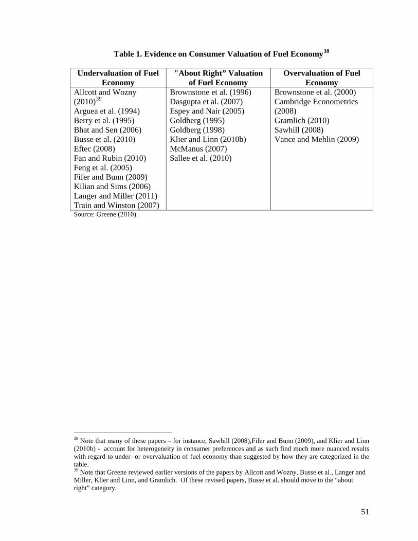
51

Table 1. Evidence on Consumer Valuation of Fuel Economy38

Undervaluation of Fuel Economy

"About Right” Valuation of Fuel Economy

Overvaluation of Fuel Economy

Allcott and Wozny (2010)39

Arguea et al. (1994)

Berry et al. (1995) Bhat and Sen (2006) Busse et al. (2010) Eftec (2008) Fan and Rubin (2010) Feng et al. (2005) Fifer and Bunn (2009) Kilian and Sims (2006) Langer and Miller (2011) Train and Winston (2007)

Brownstone et al. (1996) Dasgupta et al. (2007) Espey and Nair (2005) Goldberg (1995) Goldberg (1998) Klier and Linn (2010b) McManus (2007) Sallee et al. (2010)

Brownstone et al. (2000) Cambridge Econometrics (2008) Gramlich (2010) Sawhill (2008) Vance and Mehlin (2009)

Source: Greene (2010).

38 Note that many of these papers – for instance, Sawhill (2008),Fifer and Bunn (2009), and Klier and Linn (2010b) - account for heterogeneity in consumer preferences and as such find much more nuanced results with regard to under- or overvaluation of fuel economy than suggested by how they are categorized in the table. 39 Note that Greene reviewed earlier versions of the papers by Allcott and Wozny, Busse et al., Langer and Miller, Klier and Linn, and Gramlich. Of these revised papers, Busse et al. should move to the “about right” category.

52

Table 2. Summary of Main Sources of Variation in Vehicle Choice Models

Model Characteristics Methods

Estimated models Nested Logit Mixed Logit Two-stage methods to address endogeneity

Calibrated models Consumer Data

Individual purchaser (micro) data Vehicle sales data Aggregate (macro) data Combined micro and aggregate data

Choices included in model * Only market shares New vehicle sales Used vehicle sales Vehicle miles traveled

Market Assumptions Supply side market structure

Competitive Oligopoly

Fuel economy market structure Equilibrium in fuel economy choice Possible disequilibrium in fuel economy choice

Inclusion of Fuel Economy in Regression Fuel economy as explanatory variable Fuel cost (price per mile or miles per dollar) as explanatory variable Vehicle purchase price less exogenously calculated fuel costs (both in either present value or annualized terms) as explanatory variable Tradeoffs with other attributes explicitly modeled

* Note: There is wide variation in other included and excluded variables.

53

References ACEEE (2007). “Environmental Performance Labels for Vehicles: Context and Findings of Market Research for the U.S. Environmental Protection Agency.” Report T071. Agarwal, M. and B. Ratchford (1980). “Estimating Demand Functions for Product Characteristics: The Case of Automobiles,” Journal of Consumer Research: 249-62. Akerloff, G. (1970). “The Market for ‘Lemons:’ Quality Uncertainty and the Market Mechanisms,” Quarterly Journal of Economics 84 (3): 488-500. Allcott, H. (2010). “Beliefs and Consumer Choice.” Working Paper, Massachusetts Institute of Technology. Accessed 3/30/11. Allcott, H., and E. Muehlegger (2008). “Refining Equilibria in Counterfactual Simulations: An Application to Corporate Average Fuel Economy Standards.” Working Paper. Accessed 7/24/09. Allcott, H., and N. Wozny (2010). “Gasoline Prices, Fuel Economy, and the Energy Paradox.” Center for Energy and Environmental Policy Research Working Paper 10-003, Massachusetts Institute of Technology. Accessed 3/23/11. Anderson, S., R. Kellogg, and J. Sallee (2011a). “What Do Consumers Believe About Future Gasoline Prices?” American Economic Review: Papers and Proceedings 101 (2). Anderson, S., R. Kellogg, J. Sallee, and R. Curtin (2011b). “Forecasting Gasoline Prices Using Consumer Surveys.” Working Paper, University of Chicago. Accessed 03/01/11. Arguea, N., C. Hsiao, and G. Taylor (1994). “Estimating Consumer Preferences Using Market Data--An Application to U.S. Automobile Demand,” Journal of Applied Econometrics 9 (1): 1-18 Attanasio, O., P. Goldberg, and E. Kyriazidou (2008). “Credit Constraints in the Markets for Consumer Durables: Evidence from Micro Data on Car Loans,” International Economic Review 49 (2): 401-436. Austin, D., and T. Dinan (2005). “Clearing the Air: The Costs and Consequences of Higher CAFE Standards and Increased Gasoline Taxes,” Journal of Environmental Economics and Management 50: 562-582. Bento, A., L. Goulder, E. Henry, M. Jacobsen, and R. von Haefen (2005). “Distributional and Efficiency Impacts of Gasoline Taxes: An Econometrically Based Multi-Market Study,” American Economic Review 95(2): 282-287.

54

Bento, A., L. Goulder, M. Jacobsen, and R. von Haefen (2009). “Distributional and Efficiency Impacts of Increased U.S. Gasoline Taxes,” American Economic Review 99(3): 667-699. Benartzi, S. and R. Thaler (1995). “Myopic Loss Aversion and the Equity Premium Puzzle,” Quarterly Journal of Economics 110(1): 73-92. Berry, S., J. Levinsohn, and A. Pakes (1995). “Automobile Prices in Market Equilibrium,” Econometrica 63(4): 841-940. Berry, S., J. Levinsohn, and A. Pakes (2004). “Differentiated Products Demand Systems from a Combination of Micro and Macro Data: The New Car Market,” Journal of Political Economy 112(1): 68-105. Bhat, C., and S. Sen (2006). “Household Vehicle Type Holdings and Usage: An Application of the Multiple Distrete Continuous Extreme Value (MDCEV) Model,” Transportation Research Part B 40: 35-53. Bordley, R. (1993). “Estimating Automotive Elasticities from Segment Elasticities and First Choice/Second Choice Data,” Review of Economics and Statistics 75(3): 455-462. Brenkers, R., and F. Verboven (2006). “Liberalizing a Distribution System: The European Car Market,” Journal of the European Economic Association 4, 1: 216-251. Bresnahan T., S. Stern, and M. Trajtenberg (1997). “Market Segmentation and the Sources of Rents from Innovation: Personal Computers in the Late 1980s,” Rand Journal of Economics 28: S17-S44. Brownstone, D., D. Bunch, T. Golob, and W. Ren (1996). “A Transactions Choice Model for Forecasting Demand for Alternative-Fuel Vehicles,” Research in Transportation Economics, 4: 87-129. Brownstone, D., D. Bunch, and K. Train (2000). “Joint Mixed Logit Models of Stated and Revealed Preferences for Alternative-Fuel Vehicles,” Transportation Research Part B 34: 315-338 Brownstone, D., and K. Train (1999). “Forecasting New Product Penetration with Flexible Substitution Patterns,” Journal of Econometrics 89: 109-129. Busse, M., C. Knittel, and F. Zettelmeyer (2010). “Pain at the Pump: The Effect of Gasoline Prices on New and Used Automobile Markets,” Working Paper, University of California at Davis. Accessed 3/23/11. Cambridge Econometrics (2008). Demand for Cars and Their Attributes. Final Report. Prepared for the Department of Transport, U.K.

55

Carlsson, F., O. Johansson-Stenman and P. Martinsson (2007). “Do You Enjoy Having More than Others? Survey Evidence of Positional Goods,” Economica 74: 586-598. Congressional Budget Office (2008). Effects of Gasoline Prices on Driving Behavior and Vehicle Markets. Court, A. (1939). “Hedonic Price Indexes with Automotive Examples,” in The Dynamics of Automobile Demand, General Motors Corporation, New York: 99-117. Dasgupta, S., S. Siddarth, and J. Silva-Risso (2007). “To Lease or to Buy? A Structural Model of a Consumer’s Vehicle and Contract Choice Decisions,” Journal of Marketing Research 44: 490 – 502. Dreyfus, M., and W. Viscusi (1995). “Rates of Time Preference and Consumer Valuations of Automobile Safety and Fuel Efficiency,” Journal of Law and Economics 38 (1): 79-105 Eftec (2008). Demand for Cars and Their Attributes. Final Report. Prepared for the Department of Transport. U.K. Energy Information Administration (1996). Issues in Midterm Analysis and Forecasting 1996, DOE/EIA-0607(96). U.S. Department of Energy (DOE), Washington, D.C. Energy Information Administration (2001). Transportation Energy Consumption Survey. U.S. Department of Energy (DOE), Washington, D.C. Espey, M., and S. Nair (2005). “Automobile Fuel Economy: What is it Worth?” Contemporary Economic Policy 23(3): 317-323. Fan, Q., and J. Rubin (2010). “Two-Stage Hedonic Price Model for Light-Duty Vehicles: Consumers Valuations of Automotive Fuel Economy in Maine,” Transportation Research Record 2157: 119-128. Feng, Y., D. Fullerton, and L. Gan (2005), “Vehicle Choices, Miles Driven and Pollution Policies,” National Bureau of Economic Research Working Paper 11553. Fifer, D., and N. Bunn (2009). “Assessing Consumer Valuation of Fuel Economy in Auto Markets.” Undergraduate thesis, Duke University. Accessed 9/29/10. Fischer, C. (2004). “Who Pays for Energy Efficiency Standards?” Resources for the Future Discussion Paper, 04-11 Fischer, C., W. Harrington, and I. Parry (2007). “Should Automobile Fuel Economy Standards Be Tightened?” Energy Journal 28 (4): 1 – 29.

56

Frank, R. (1985). “The Demand for Unobservable and Other Nonpositional Goods,” American Economic Review 75(1): 101-116. Frank, R., and C. Sunstein (2001). “Cost-Benefit Analysis and Relative Position,” The University of Chicago Law Review 68(2): 323-374. Freeman III, A.M. (2003). The Measurement of Environmental and Resource Values: Theory and Methods. Washington, D.C.: Resources for the Future. Goldberg, P. (1995). “Product Differentiation and Oligopoly in International Markets: The Case of the U.S. Automobile Industry,” Econometrica 63(4): 891-951. Goldberg, P. (1998). “The Effects of the Corporate Average Fuel Efficiency Standards in the U.S.” Journal of Industrial Economics 46(1): 1-33. Gramlich, J. (2010). “Gas Prices, Fuel Efficiency, and Endogenous Product Choice in the U.S. Automobile Industry,” Working Paper, Yale University. Accessed 3/23/11. Greene D. (2001). “TAFV Alternative Fuels and Vehicles Choice Model Documentation,” prepared by the Oak Ridge National Laboratory for the U.S. Department of Energy. Greene, D. (2009a). “Feebates, Footprints and Highway Safety,” Transportation Research Part D 14: 375-384. Greene, D. (2010). “How Consumers Value Fuel Economy: A Literature Review.” Office of Transportation and Air Quality, U.S. Environmental Protection Agency, Report EPA-420-R-10-008. Greene, D. (2011). “Uncertainty, Loss Aversion, and Markets for Energy Efficiency,” Energy Economics, forthcoming. Greene, D., K. Duleep, D. Elliott, and S. Ahmad (2005a). “A Fuel Economy Regulatory Analysis Model (FERAM) For the Energy Information Administration,” prepared by Oak Ridge National Laboratory for U.S. Department of Energy. Greene, D., K. Duleep, and W. McManus (2004). “Future Potential of Hybrid and Diesel Powertrains in the U.S. Light-Duty Vehicle Market,” prepared by the Oak Ridge National Laboratory for the U.S. Department of Energy. Greene, D., J. German, and M. Delucchi (2009b). “Fuel Economy: The Case for Market Failure” in Reducing Climate Impacts in the Transportation Sector, Sperling, D., and J. Cannon, eds. Springer Science. Greene, D., L. Goeltz, J. Hopson, and E. Tworek (2006). “Analysis of In-Use Fuel Economy Shortfall by Means of Voluntarily Reported Fuel Economy Estimates.” Transportation Research 1983. Transportation Research Board, Washington, DC.

57

Greene, D., and J. Liu (1988). “Automotive Fuel Economy Improvements and Consumers’ Surplus,” Transportation Research Part A 22A(3): 203-218. Greene, D., P. Patterson, M. Singh, and J. Li (2005b). “Feebates, Rebates, and Gas-Guzzler Taxes: A Study of Incentives for Increased Fuel Economy,” Energy Policy 33: 757-775. Greene, William (2008). Econometric Analysis. Sixth Edition. Prentice Hall. Haab, T., and K. McConnell (2002). Valuing Environmental and Natural Resources: The Econometrics of Non-Market Valuation. Northampton, MA: Edward Elgar. International Council on Clean Transportation (2010). “Global Passenger Car Fuel Economy and/or Greenhouse Gas Emissions Standards, April 2010 Update.” Accessed 9/28/10. IEA (2007). Mind the Gap: Quantifying Principal-Agent Problems in Energy Efficiency. Paris, France: International Energy Agency. Jacobsen, M. (2010). “Evaluating U.S. Fuel Economy Standards in a Model with Producer and Household Heterogeneity,” Working Paper, University of California, San Diego. Accessed 3/23/11. Jaffe, A, R. Newell, and R. Stavins (2001). "Energy Efficient Technologies and Climate Change Policies: Issues and Evidence." In Climate Change Economics and Policy, Toman, Michael A., ed., Washington, D.C.: Resources for the Future. p.171 - 181. Kilian, L., and E. Sims (2006). “The Effects of Real Gasoline Prices on Automobile Demand: A Structural Analysis Using Micro Data.” Working Paper, Notre Dame. Accessed 09/30/10. Kleit, A. (2004). “Impacts of Long-Range Increases in the Fuel Economy (CAFE) Standard,” Economic Inquiry 42(2): 279-294. Klier, T., and J. Linn (2010a). “New Vehicle Characteristics and the Cost of the Corporate Average Fuel Economy Standard,” Resources for the Future Discussion Paper 10-50. Klier, T., and J. Linn (2010b). “The Price of Gasoline and New Vehicle Fuel Economy: Evidence from Monthly Sales Data,” American Economic Journal: Economic Policy 2(3): 134-153. Knittel, C. (forthcoming). “Automobiles on Steroids: Product Attribute Trade-Offs and Technological Progress in the Automobile Sector,” American Economic Review.

58

Knittel, C., and K. Metaxoglou (2008). “Estimation of Random Coefficient Demand Models: Challenges, Difficulties and Warnings.” National Bureau of Economic Research Working Paper 14080. Kubik, M. (2006). Consumer Views on Transportation and Energy. Second Edition. Technical Report: National Renewable Energy Laboratory. Langer, A., and N. Miller (2011). “Automakers’ Short Run Responses to Changing Gasoline Prices and the Implications for Energy Policy.” Working Paper, University of Michigan. Accessed 3/23/11. Larrick, R., and J. Soll (2008). “The MPG Illusion,” Science 320: 1593-1594. Li, S., C. Timmins, and R. von Haefen (2009). “How Do Gasoline Prices Affect Fleet Fuel Economy?” American Economic Journal: Economic Policy 1(2): 113-137. McManus, W. (2006). “Can Proactive Fuel Economy Strategies Help Automakers Mitigate Fuel-Price Risks?” Working Paper, University of Michigan Transportation Research Institute. McManus, W. (2007). “The Impact of Attribute-Based Corporate Average Fuel Economy (CAFE) Standards: Preliminary Findings.” University of Michigan Transportation Research Institute Paper UMTRI-2007-31. McManus, W. and R. Kleinbaum (2009). “Fixing Detroit: How Far, How Fast, How Fuel Efficient.” Working Paper, Transportation Research Institute, University of Michigan. Metcalf, G., and K. Hassett (1999). "Measuring the Energy Savings From Home Improvement Investments: Evidence From Monthly Billing Data," The Review of Economics and Statistics 81(3): 516-528. Metcalf, G., and D. Rosenthal (1995). "The ‘New’ View of Investment Decisions and Public Policy Analysis: An Application to Green Lights and Cold Refrigerators,” Journal of Policy Analysis and Management 14: 517–531. Mohammadian, A., and E. Miller (2003). “Empirical Investigation of Household Vehicle Type Choice Decisions,” Transportation Research Record 1854: 99-106. NERA Economic Consulting (2008). “Evaluation of NHTSA’s Benefit-Cost Analysis of 2011-2015 CAFE Standards.” Nevo, A. (2000). ”A Practitioner’s Guide to Estimation of Random Coefficients Logit Models of Demand,” .Journal of Economics & Management Strategy 9(4): 513-548. Nevo, A. (2001). “Measuring Market Power in the Ready-to-Eat Cereal Industry,” Econometrica 69 (2): 307-342.

59

Ohta, M., and Z. Griliches (1986). “Automobile Prices and Quality: Did the Gasoline Price Increases Change Consumer Tastes in the U.S.?” Journal of Business and Economic Statistics 4: 187-98. Petrin, A. (2002). “Quantifying the Benefits of New Products: The Case of the Minivan,” Journal of Political Economy 110: 705-729. PRR, Inc. (2005), “EPA Fuel Economy Label Focus Groups: Report of Findings,” Prepared for the USEPA. Sallee, J., S. West, and W. Fan (2010). “The Effect of Gasoline Prices on the Demand for Fuel Economy in Used Vehicles: Empirical Evidence and Policy Implications,” Working Paper Version 1.2, University of Chicago. Sanstad, A., and R. Howarth (1994). “’Normal’ Markets, Market Imperfections, and Energy Efficiency,” Energy Policy 22(10): 811-818. Sawhill, J. (2008). “Are Capital and Operating Costs Weighted Equally in Durable Good Purchases? Evidence from the U.S. Automobile Market.” Discussion Paper, University of California at Berkeley. April. Shogren, J., and L. Taylor (2008). “On Behavioral-Environmental Economics,” Review of Environmental Economics and Policy 2, 1: 26 – 44. Simon, H. (1955). “A Behavioral Model of Rational Choice,” Quarterly Journal of Economics 69(1): 99-118. Spissu, E., A. Pinjari, R. Pendyala, and C. Bhat (2009). “A Copula-Based Joint Multinomial Discrete-Continuous Model of Vehicle Type Choice and Miles of Travel,” Transportation 36(4): 403-422. Teisl, M., C. Noblet, and J. Rubin (2009). “Can Environmental Promotion Backfire? Evidence from the Vehicle Market,” Social Marketing Quarterly 15(3): 2-32. Tietenberg, T. (2009). “Reflections – Energy Efficiency Policy: Pipe Dream or Pipeline to the Future?” Review of Environmental Economics and Policy 3 (2): 304 -320. Train, K. (2009). Discrete Choice Methods with Simulation, Second Edition. New York: Cambridge University Press. Train, K., and Clifford Winston (2007). “Vehicle Choice Behavior and the Declining Market Share of U.S. Automakers,” International Economic Review 48: 1469-1496. Turrentine, T., and K. Kurani (2007). “Car Buyers and Fuel Economy?” Energy Policy 35: 1213-1223.

60

Tversky, A., and D. Kahneman (1991). “Loss Aversion in Riskless Choice: A Reference Dependent Model,” The Quarterly Journal of Economics 106, 4: 1039 – 61. Vance, C., and M. Mehlin (2009). “Tax Policy and CO2 Emissions: An Econometric Analysis of the German Automobile Market.” Ruhr Economic Papers #89, RWi Essen, Germany. U.S. Environmental Protection Agency and Department of Transportation (2010a). “Light-Duty Vehicle Greenhouse Gas Emission Standards and Corporate Average Fuel Economy Standards; Final Rule.” Federal Register 75(88): 25323-25728. U.S. Environmental Protection Agency and Department of Transportation (2010b). “Revisions and Additions to Motor Vehicle Fuel Economy Label; Proposed Rule.” Federal Register 75(184): 58078-58202. West, S. (2008). “The Effect of Gasoline Prices on the Demand for Sport Utility Vehicles.” Working Paper, Macalester College, Whitefoot, K., M. Fowlie, and S. Skerlos (2011). “Product Design Response to Industrial Policy: Evaluating Fuel Economy Standards Using an Engineering Model of Endogenous Product Design.” Working Paper, University of Michigan. Accessed 3/23/11.