Evaluating an active learning approach to teaching introductory

Journal of Statistics Education, Volume 19, Number 1 (2011)

1

Evaluating an active learning approach to teaching introductory

statistics: A classroom workbook approach

Kieth A. Carlson

Jennifer R. Winquist

Valparaiso University

Journal of Statistics Education Volume 19, Number 1 (2011),

www.amstat.org/publications/jse/v19n1/carlson.pdf

Copyright © 2011 by Kieth A. Carlson and Jennifer R. Winquist all rights reserved. This text

may be freely shared among individuals, but it may not be republished in any medium without

express written consent from the authors and advance notification of the editor.

Key Words: Active learning; Student attitudes; Curriculum assessment; Course evaluation;

Instructor immediacy.

Abstract

The study evaluates a semester-long workbook curriculum approach to teaching a college level

introductory statistics course. The workbook curriculum required students to read content before

and during class and then work in groups to complete problems and answer conceptual questions

pertaining to the material they read. Instructors spent class time answering students’ questions.

The 59 students who experienced the workbook curriculum completed the Survey of Attitudes

Toward Statistics (SATS) on the first and last day of the course. These students’ post course

ratings on the subscales of cognitive competence, affect and difficulty were all significantly

higher than their pre course ratings. Additionally, the 59 students’ post course ratings for these 3

subscales were also significantly higher than those provided by a comparison group of statistics

students (sample size 235). The results indicated that the students experiencing the workbook

curriculum (1) had more confidence in their ability to perform and understand statistics, (2) liked

statistics more, and (3) thought statistics was more difficult than the comparison group.

Additionally, these students’ attitude scores were positively correlated with both GPA and

performance on a comprehensive final exam. We discuss the various methodological problems

faced by classroom researchers and suggest that, in some cases, assessing students’ attitudes can

be an effective solution to these methodological problems. We conclude that the workbook

approach holds promise for teaching introductory statistics courses.


2

1. Introduction

1.1 Student attitudes and course evaluation

Measuring students’ attitudes toward statistics both before and after completing a course is one

way to assess a statistics curriculum’s effectiveness (Harlow, Buckholder and Marrow, 2002;

Manning, Zachar, Ray and Lo Bello, 2006; Sizemore and Lewandowski, 2009). Not only is

attitude change an important outcome in its own right, but student attitudes toward statistics

before and/or after taking a statistics course are also associated with other outcome variables.

Specifically, more positive attitudes are associated with better performance in the course (Chiesi

and Primi, 2009; Elmore, Lewis and Bay, 1993; Finney and Schraw, 2003; Roberts and Saxe,

1982; Schau, 2003, Schutz, Drogosz, White, and Distefano, 1998; Sorge and Schau, 2002) as

well as increased future enrollment in additional statistics courses (Finney and Schraw, 2003).

The published classroom research that measures the change in students’ attitudes toward

statistics across a semester is mixed. Harlow et al. (2002) reported that their participants had

significantly more positive attitudes about statistics after completing a statistics course.

Specifically, their students had greater quantitative self-efficacy and significantly less

quantitative anxiety. DeVaney (2010) found that students who took a graduate course online

reported a decrease in statistics class anxiety and an increase in affect toward statistics but

students who took the same course on campus did not report less anxiety or greater affect at the

end of the course. It is noteworthy that the positive changes in attitude were small and only

occurred in the online course in which initial anxiety was higher. Other researchers have also

found mixed results. In their validation study, Cashin and Elmore (2005) used the Survey of

Attitudes Toward Statistics Scale (SATS), the Attitude Toward Statistics Scale (ATS), and the

Statistics Attitude Survey (SAS) to measure 342 students’ attitudes toward statistics both before

and after completing a statistics course. The SATS and the ATS each have subscales that

measure different kinds of attitudes towards statistics (e.g., Affect, Cognitive Competence,

Difficulty, Value, Effort, Course, and Field). Considering the subscales as distinct metrics the

validation study actually measured seven different student attitudes both before and after a

course. Only two of the seven attitudes were more positive after the course. Specifically, the

students showed a positive attitude change on the ATS Course subscale which contained items

like “I would like to continue my statistical training in an advanced course.” Students also

scored more positively on the SATS Affect scale which contained items like “I like statistics”

and “I feel insecure when I have to do statistics problems,” (reverse-keyed). The remaining five

attitude measures showed no change. Further, the effect sizes for the two observed changes were

both small.

It is clear that the statistics courses evaluated in the literature had different effects on students’

attitudes toward statistics. Further, given the diversity of the results it is not possible to say what

impact taking a statistics course has on students’ attitudes. Knowing details about how these

courses were taught (i.e., their respective course structures) might help explain these divergent

results. [See Finney and Schraw (2003) for a detailed discussion of how using general versus

task specific measures of self efficacy might also explain some of these divergent results].


3

1.2 Evaluating active learning approaches

Just as there are divergent results with respect to how a statistics course impacts students’

attitudes toward statistics there are also divergent results with respect to the effectiveness of

“active learning approaches” when teaching statistics. Some instructors/researchers have

presented anecdotal evidence suggesting that active learning is effective (e.g., Knypstra, 2009;

Bates Prins, 2009) and others have presented evidence that students’ exam scores are higher

when taught with an active learning approach than when taught with more traditional approaches

(e.g., Christopher and Marek, 2009; Steinhorst and Keeler, 1995; Ryan, 2006; Yoder and

Hochevar, 2005). Although numerous studies have found active learning to be effective, others

have found it to have no effect (e.g., Pfaff and Weinberg, 2009) or even to hinder student

performance (e.g., Weltman and Whiteside, 2010).

One of the reasons for the inconsistent results in the active learning literature is the enormous

diversity of approaches that are referred to as “active learning.” The only unifying characteristic

seems to be that students are asked to “do something” (Page, 1990). We suspect that most

advocates of active learning would not suggest that educators can have students “do anything”

and expect positive results. Certainly, what students do and how they think about what they did

determines whether a given active learning approach will be successful. For example, Pfaff and

Weinberg (2009) held the view that actively generating data (and then analyzing that data) would

increase students’ understanding of the statistical concepts that underlie the statistical

computations. They created clever hands-on data generation activities in which their students

used cards to illustrate the central limit theorem as well as rolled dice and drew chips to compute

confidence intervals. During each of these activities their students were asked some

computational and/or conceptual questions but the primary focus was on generating data for the

computations not on explaining underlying statistical concepts. After the hands-on data

collection activities students’ understanding of the underlying statistical concepts was assessed.

Despite the fact that their students actively generated data, their students’ post activity

assessment performance was not better than their pre activity performance. We believe that Pfaff

and Weinberg (2009) were correct to conclude that the physical act of generating data was not

sufficient to produce learning. However, we do not think it is correct to conclude from their

study that active learning approaches in general are ineffective.

In our view, active learning activities are effective to the degree that they encourage students to

think about the underlying statistical concepts. If we are correct in this assertion, Pfaff and

Weinberg’s (2009) activities may have been ineffective because the data collection exercises

were not used to explain underlying statistical concepts. Pfaff and Weinberg (2009) recognized

this possibility in their discussion when they stated, “. . .when we use the modules in the future,

we plan on giving students follow-up activities that have them spend more time describing key

aspects of the concepts.” If these same data collection activities included narratives that

explained how the cards, dice, and chips illustrated key statistical concepts and students were

required to answer questions about each concept as they performed each operation, it is possible

that the activities would be more effective. We suspect that the key components of successful

active learning approaches are using activities to explain concepts and requiring students to

demonstrate that they understand these concepts by having them answer very specific rather than

general questions.


4

Weltman and Whiteside (2010) were even more critical of active learning approaches than Pfaff

and Weinberg (2009). They recently reported evidence that two active learning approaches were

not only ineffective but also detrimental to some students. These divergent results might also be

explained by analyzing the details of their study. Weltman and Whiteside (2010) compared three

different ways of teaching binomial distributions, sampling distributions and calculating p-values

in hypothesis testing. Seven sections of undergraduate business students were taught each of the

above course topics with a traditional lecture, a hybrid presentation method, or an experiential

learning method. The traditional method involved instructors presenting slides to students

verbally. The hybrid method involved instructors presenting the same lecture slides in the same

manner but with pauses after 15 minutes of lecture in which students were asked to answer

questions pertaining to the previous 15 minute lecture. The active learning method involved

students working in groups of two or three using “documentation . . . developed by the

researcher.” For example, pairs of students used “software that interactively display[ed]

sampling distributions from different population distributions for selected sample sizes.” After

experiencing one of these teaching methods all students took a common 20 minute multiple

choice quiz to measure what they learned.

Weltman and Whiteside (2010) reported an interaction between teaching method and student

GPA. When the lecture method was used the performance of high, medium and low GPA

students was significantly different as would be expected. However when the hybrid and “fully

active” approaches were used, students with high, medium and low GPAs performed equally. In

both conditions the performance of the high GPA students was significantly less than their

performance under the lecture method.

The authors concluded, “that active learning is not universally effective and, in fact, it may

inhibit learning for certain types of students.” Further, they concluded, “It is possible that

students with a high grade point average achieve a deeper level of learning when experiencing

exposure to the maximum amount of instructor expertise and direction.” Weltman and

Whiteside’s (2010) results clearly illustrate their high GPA students performed worse under their

hybrid and “fully active” conditions. Obviously, these results challenge much of the anecdotal

evidence used to support the effectiveness of “active learning” approaches to education. While

the “active learning” methods evaluated by Weltman and Whiteside (2010) were not effective for

all students, even detrimental to some, it is possible that other active learning methods are

effective for all students.

Our study had three purposes: (1) to evaluate the effectiveness of a semester-long active learning

statistics curriculum that differed significantly from the single day activities found ineffective by

Weltman and Whiteside (2010), (2) to evaluate this active learning curriculum’s impact on

students’ attitudes toward statistics, and (3) to determine if this active learning curriculum had a

detrimental effect on the performance of high GPA students.


5

2. Research Design

2.1 Survey of Attitudes Toward Statistics (SATS-36)

We used the SATS-36 (Schau, Stevens, Dauphinee, and Del Vecchio, 1995) to measure students’

attitudes toward statistics. Students completed the SATS on the first and last day of class. The

SATS-36 is a 36 item scale with six subscales. Cronbach’s alphas (α) were computed for each

subscale using the pre test and post test data. Scales are generally considered reliable if α is at

least .7 (Field, 2009). The six item affect subscale assessed students’ feelings toward statistics

(e.g., I will like statistics; I am scared by statistics) (pre test α = .88, post test α = .87). The six

item cognitive competence subscale assessed students’ beliefs about their ability to understand

statistics (e.g., I can learn statistics; I will have trouble understanding statistics because of how I

think) (pre test α = .93, post test α = .86.). The seven item difficulty subscale assessed students’

beliefs about the difficulty of statistics (e.g., Statistics formulas are easy to understand; Statistics

is a complicated subject) (pre test α = .91, post test α = .81). The four item interest subscale

assessed students’ interest in statistics (e.g., I am interested in being able to communicate

statistical information to others; I am interested in using statistics) (pre test α = .89, post test α =

.84). The four item effort subscale assessed students’ beliefs about the amount of effort they

would/did put in to the class (e.g., I plan to complete all of my statistics assignments; I plan to

work hard in my statistics course) (pre test α = .83, post test α = .71). The nine item value

subscale assessed students’ beliefs about the usefulness of statistics in their lives (e.g., Statistics

is worthless; Statistics should be a required part of my professional training) (pre test α = .85,

post test α = .58). Although our reliability coefficient for the value subscale on the post test is

low in our data, the scale has been shown to have adequate internal reliability in previous

research (Cashin and Elmore, 2005; Hilton, Schau, and Olsen, 2004). All 36 SATS items use a

7-point likert scale (e.g., 1 = Strongly disagree to 7 = Strongly agree). Higher SATS scores

indicate more positive attitudes toward statistics.

2.2 Students

Of the 86 students who enrolled in four sections of an introductory statistics course 59 completed

both the pre SATS and post SATS. Sixteen students completed only the pre test, six completed

only the post test, and five did not complete either test. Students who completed both surveys did

not have significantly different GPAs than students who did not complete both surveys, t(71) =

.83, p = .40, η2 = .01, nor did they have significantly different scores on the final exam, t (83) =

.57, p = .57, η2 = .004. The 16 students who completed only the pre SATS were not significantly

different from those 59 students who completed both on any pre SATS subscale nor did they

differ on the final exam (all test statistics < 1 and p-values > .36).

Of the 59 students included in subsequent analyses, 15 were nursing majors, 11 were psychology

majors, 11 were sociology/social work majors, 6 were pre med, 5 were biology majors, 3 were

physical education, 2 were chemistry majors, 2 were Arts/Humanities majors, 1 was an education

major and 3 students did not yet have a major. The mean age was 21.3 (SD = 5.4, median = 20,

mode = 20). Thirteen students were male and 46 were female.


6

2.3 Class Structure

Four sections of approximately 22 students each were taught by two instructors. One instructor

taught 3 sections of the course. The course covered the topics typically covered in a

behavioral/social sciences statistics course. Specifically, the course included units on frequency

distributions, central tendency, variability, z scores, z-tests, t-tests, oneway ANOVAs, factorial

ANOVAs and correlations. All computations were performed using a calculator and/or a

computer software package (i.e., PASW/SPSS).

Prior to class students read a short chapter (approximately five pages, single spaced) introducing

the topic. These chapters were written specifically for this course and included a conceptual

explanation of the topic, a completed computational example problem and an example of how to

summarize the results of the analysis. After reading this information students were required to

answer questions about the reading, to complete a computational problem, and to summarize the

results of their computations. These questions were intended to be relatively simple and did not

require application of the material. Answers to these problems were submitted prior to class via

an online course management system. Students received feedback about their performance prior

to class and were allowed to correct errors on homework questions. These homework

assignments collectively accounted for approximately 17% of students’ course grades.

The class period began with the instructor answering questions about the homework assignment,

giving a brief lecture that reviewed the information in the reading, and introducing the activity

for that day. The length of the lecture varied depending on student questions and the difficulty of

the activity, but was typically 15-20 minutes. Class sessions were 75 minutes long occurring

twice a week.

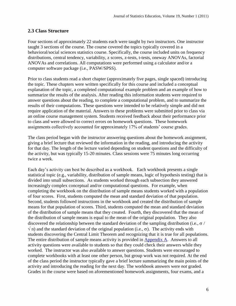
Each day’s activity can best be described as a workbook. Each workbook presents a single

statistical topic (e.g., variability, distribution of sample means, logic of hypothesis testing) that is

divided into small subsections. As students worked through each subsection they answered

increasingly complex conceptual and/or computational questions. For example, when

completing the workbook on the distribution of sample means students worked with a population

of four scores. First, students computed the mean and standard deviation of that population.

Second, students followed instructions in the workbook and created the distribution of sample

means for that population of scores. Third, students computed the mean and standard deviation

of the distribution of sample means that they created. Fourth, they discovered that the mean of

the distribution of sample means is equal to the mean of the original population. They also

discovered the relationship between the standard deviation of the sampling distribution (i.e., /

n) and the standard deviation of the original population (i.e., ). The activity ends with

students discovering the Central Limit Theorem and recognizing that it is true for all populations.

The entire distribution of sample means activity is provided in Appendix A. Answers to all

activity questions were available to students so that they could check their answers while they

worked. The instructor was also available to answer questions. Students were encouraged to

complete workbooks with at least one other person, but group work was not required. At the end

of the class period the instructor typically gave a brief lecture summarizing the main points of the

activity and introducing the reading for the next day. The workbook answers were not graded.

Grades in the course were based on aforementioned homework assignments, four exams, and a


7

cumulative final exam. All exam questions were novel, meaning no items had occurred

previously in any homework or exam.

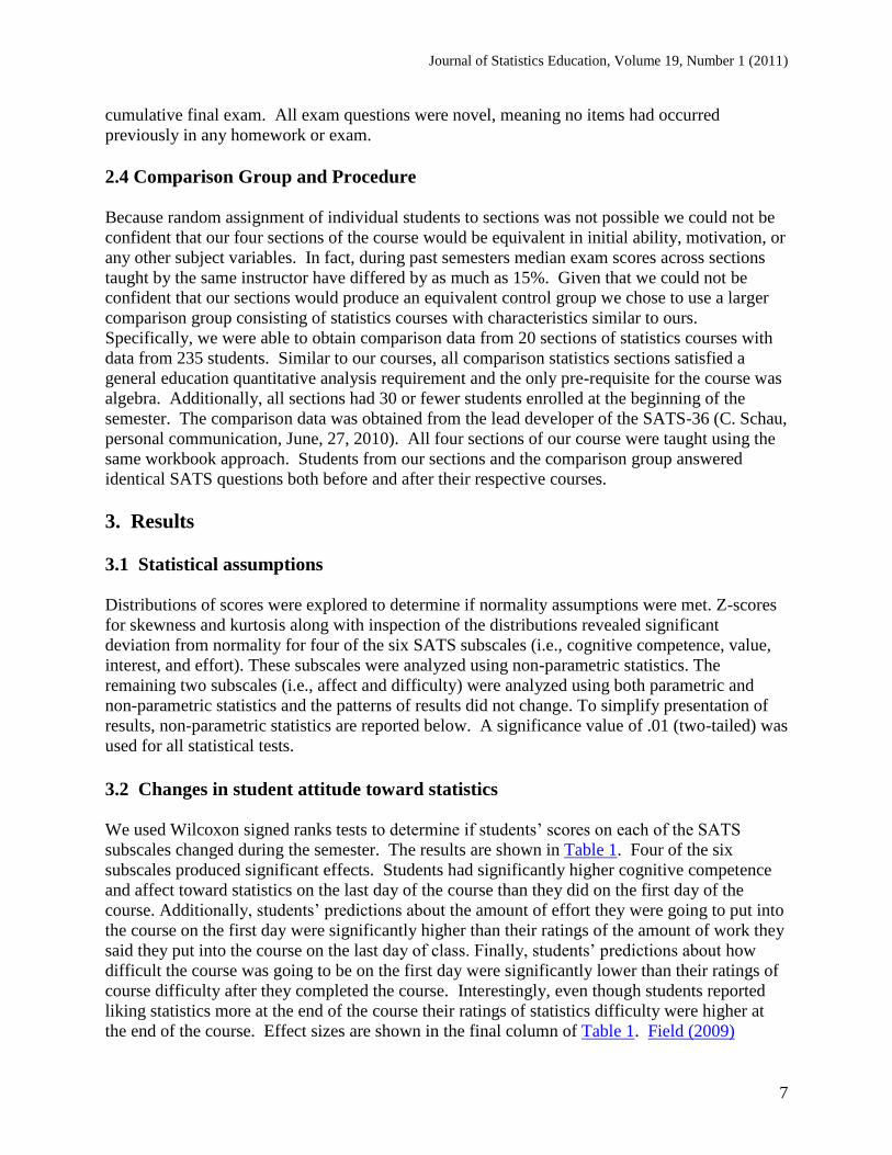
2.4 Comparison Group and Procedure

Because random assignment of individual students to sections was not possible we could not be

confident that our four sections of the course would be equivalent in initial ability, motivation, or

any other subject variables. In fact, during past semesters median exam scores across sections

taught by the same instructor have differed by as much as 15%. Given that we could not be

confident that our sections would produce an equivalent control group we chose to use a larger

comparison group consisting of statistics courses with characteristics similar to ours.

Specifically, we were able to obtain comparison data from 20 sections of statistics courses with

data from 235 students. Similar to our courses, all comparison statistics sections satisfied a

general education quantitative analysis requirement and the only pre-requisite for the course was

algebra. Additionally, all sections had 30 or fewer students enrolled at the beginning of the

semester. The comparison data was obtained from the lead developer of the SATS-36 (C. Schau,

personal communication, June, 27, 2010). All four sections of our course were taught using the

same workbook approach. Students from our sections and the comparison group answered

identical SATS questions both before and after their respective courses.

3. Results

3.1 Statistical assumptions

Distributions of scores were explored to determine if normality assumptions were met. Z-scores

for skewness and kurtosis along with inspection of the distributions revealed significant

deviation from normality for four of the six SATS subscales (i.e., cognitive competence, value,

interest, and effort). These subscales were analyzed using non-parametric statistics. The

remaining two subscales (i.e., affect and difficulty) were analyzed using both parametric and

non-parametric statistics and the patterns of results did not change. To simplify presentation of

results, non-parametric statistics are reported below. A significance value of .01 (two-tailed) was

used for all statistical tests.

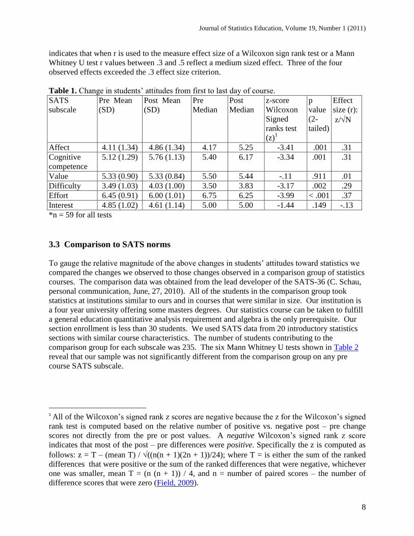
3.2 Changes in student attitude toward statistics

We used Wilcoxon signed ranks tests to determine if students’ scores on each of the SATS

subscales changed during the semester. The results are shown in Table 1. Four of the six

subscales produced significant effects. Students had significantly higher cognitive competence

and affect toward statistics on the last day of the course than they did on the first day of the

course. Additionally, students’ predictions about the amount of effort they were going to put into

the course on the first day were significantly higher than their ratings of the amount of work they

said they put into the course on the last day of class. Finally, students’ predictions about how

difficult the course was going to be on the first day were significantly lower than their ratings of

course difficulty after they completed the course. Interestingly, even though students reported

liking statistics more at the end of the course their ratings of statistics difficulty were higher at

the end of the course. Effect sizes are shown in the final column of Table 1. Field (2009)


8

indicates that when r is used to the measure effect size of a Wilcoxon sign rank test or a Mann

Whitney U test r values between .3 and .5 reflect a medium sized effect. Three of the four

observed effects exceeded the .3 effect size criterion.

Table 1. Change in students’ attitudes from first to last day of course.

SATS

subscale

Pre Mean

(SD)

Post Mean

(SD)

Pre

Median

Post

Median

z-score

Wilcoxon

Signed

ranks test

(z)1

p

value

(2-

tailed)

Effect

size (r):

z/N

Affect 4.11 (1.34) 4.86 (1.34) 4.17 5.25 -3.41 .001 .31

Cognitive

competence

5.12 (1.29) 5.76 (1.13) 5.40 6.17 -3.34 .001 .31

Value 5.33 (0.90) 5.33 (0.84) 5.50 5.44 -.11 .911 .01

Difficulty 3.49 (1.03) 4.03 (1.00) 3.50 3.83 -3.17 .002 .29

Effort 6.45 (0.91) 6.00 (1.01) 6.75 6.25 -3.99 < .001 .37

Interest 4.85 (1.02) 4.61 (1.14) 5.00 5.00 -1.44 .149 -.13

*n = 59 for all tests

3.3 Comparison to SATS norms

To gauge the relative magnitude of the above changes in students’ attitudes toward statistics we

compared the changes we observed to those changes observed in a comparison group of statistics

courses. The comparison data was obtained from the lead developer of the SATS-36 (C. Schau,

personal communication, June, 27, 2010). All of the students in the comparison group took

statistics at institutions similar to ours and in courses that were similar in size. Our institution is

a four year university offering some masters degrees. Our statistics course can be taken to fulfill

a general education quantitative analysis requirement and algebra is the only prerequisite. Our

section enrollment is less than 30 students. We used SATS data from 20 introductory statistics

sections with similar course characteristics. The number of students contributing to the

comparison group for each subscale was 235. The six Mann Whitney U tests shown in Table 2

reveal that our sample was not significantly different from the comparison group on any pre

course SATS subscale.

1 All of the Wilcoxon’s signed rank z scores are negative because the z for the Wilcoxon’s signed

rank test is computed based on the relative number of positive vs. negative post – pre change

scores not directly from the pre or post values. A negative Wilcoxon’s signed rank z score

indicates that most of the post – pre differences were positive. Specifically the z is computed as

follows: z = T – (mean T) / ((n(n + 1)(2n + 1))/24); where T = is either the sum of the ranked

differences that were positive or the sum of the ranked differences that were negative, whichever

one was smaller, mean T = (n (n + 1)) / 4, and n = number of paired scores – the number of

difference scores that were zero (Field, 2009).


9

Table 2. Comparison of pre course attitudes

SATS

subscale

Sample

Pretest

Mean (SD)

Comparison

group pretest

Mean (SD)

Sample

Pretest

Median

Comparison

group

Pretest

Median

Mann

Whitney

(z)

p

value

(2-

tailed)

Effect

size (r):

z/N

Affect 4.11 (1.34) 4.34 (1.14) 4.17 4.33 -1.14 .25 .07

Cognitive

competence

5.12 (1.29) 5.04 (.96) 5.40 5.00 -1.11 .27 .06

Value 5.33 (0.90) 5.28 (0.92) 5.50 5.33 -.81 .42 .05

Difficulty 3.49 (1.03) 3.65 (0.71) 3.50 3.71 -0.98 .33 .06

Effort 6.45 (0.91) 6.43 (0.86) 6.75 6.75 -1.02 .31 .06

Interest 4.85 (1.02) 4.90 (1.22) 5.00 5.00 -.23 .82 .01

*N = 294; our n = 59; comparison n = 235.

However, the tests shown in Table 3 reveal that our sample was significantly different from the

comparison group on 3 of the 6 post course SATS subscales (when using a significance level of

.01, two-tailed). Specifically, our sections reported liking statistics significantly more than the

comparison group did (i.e., more positive affect scores). Our students also reported significantly

higher statistical cognitive competence (i.e., confidence in their ability to understand and

perform statistical procedures) than the comparison group. While students in our sections

thought statistics was harder than the comparison group they also liked statistics more than the

comparison group.

Table 3. Comparison of post course attitudes

SATS

subscale

Sample

Posttest

Mean (SD)

Comparison

group

Posttest Mean

(SD)

Sample

Posttest

Median

Comparison

group

Posttest

Median

Mann

Whitney

(z)

p

value

(2-

tailed)

Effect

size (r):

z/N

Affect 4.86 (1.34) 4.16 (1.41) 5.25 4.17 -3.60 <.001 .21

Cognitive

Competence

5.76 (1.13) 4.93 (1.15) 6.17 5.00 -5.04 <.001 .29

Value 5.33 (0.84) 4.94 (1.20) 5.44 4.89 -2.18 .03 .13

Difficulty 4.03 (1.00) 3.63 (0.86) 3.83 3.57 -3.01 .003 .18

Effort 6.00 (1.01) 6.08 (0.96) 6.25 6.25 -.40 .62 .02

Interest 4.61 (1.14) 4.36 (1.52) 5.00 4.50 -1.01 .28 .06


The results in Table 4 revealed that our sample experienced significantly larger change scores

(i.e., post – pre) than the comparison group on three of the six SATS subscales (when using a

significance level of .01, two-tailed). Our sample experienced a greater increase in how much

they liked statistics (i.e., affect) and their confidence in their ability to perform statistics (i.e.,

cognitive competence). Interestingly, while our sample had more improved affect and cognitive

competence ratings, they also produced a greater increase in statistics difficulty ratings.


10

Table 4. Comparison of change scores

SATS

subscale

Sample

Mean

Difference

(SD)

Comparison

group Mean

Difference

(SD)

Sample

Median

Difference

Comparison

group

Median

Difference

Mann

Whitney

(z)

p

value

(2-

tailed)

Effect

size (r):

z/N

Affect .75 (1.49) -.18 (1.33) .70 -.16 -3.96 <.001 .23

Cognitive

Competence

.64 (1.39) -.12 (1.06) .50 .00 -3.79 <.001 .22

Value .00 (0.88) -.34 (1.07) .08 -.22 -1.87 .06 .11

Difficulty .53 (1.11) -.03 (0.79) .33 .00 -3.52 <.001 .21

Effort -.45 (1.13) -.35 (1.14) -.25 -.25 -.98 .33 .06

Interest -.23 (1.27) -.54 (1.27) -.25 -.50 -1.54 .12 .09


3.4 Students’ cognitive competence and performance

The students in our statistics sections reported significantly higher confidence in their ability to

perform statistics after completing the course and this increase in confidence was significantly

greater than those produced in the comparison group. An important question is whether our

students’ higher confidence with statistics is associated with better performance. We correlated

students’ pre and post cognitive competence scores with their performance on the comprehensive

final exam to address this question. The Spearman correlation between students’ pre cognitive

competence scores (i.e., students’ reported confidence with statistics on the first day of class) and

their score on the final exam explained 15% of the variance in exam performance, rS (57) = .39,

p = .002. Post cognitive competence (i.e., students’ reported confidence approximately 3 to 5

days before the final exam) explained 30% of the variance in final exam performance, rS (57) =

.55, p < .001. Clearly, our students’ self assessment of their statistics knowledge is positively

associated with their actual performance.

3.5 GPA, Student attitudes and Performance

Weltman and Whiteside (2010) found that using an activity instructional method helped the

performance of lower GPA students (GPA of 1.75 or lower) but hindered the performance of

higher GPA students (GPA of 3.75 or higher). Although Weltman and Whiteside (2010) did not

measure students’ attitudes, given that students’ level of achievement in statistics courses is

frequently positively correlated with students’ post course attitudes toward statistics (Chiesi and

Primi, 2009; Elmore, et al., 1993; Finney and Schraw, 2003; Roberts and Saxe, 1982; Schau,

2003; Schutz, Drogosz, White, and Distefano, 1998; Sorge and Schau, 2002) it would not be

surprising if a variable impacting students’ performance in a course also impacted student’s

attitudes in a similar manner. Therefore, if our active learning approaches help the performance

of lower GPA students and hinder the performance of higher GPA students one would expect a

zero or negative correlation between GPA and post course attitudes (i.e., post SATS scores).

However, we found 3 positive Spearman correlations. Specifically, after experiencing a semester

of activity based instruction, higher GPA students liked statistics more, rS (57) = .32, p = .02,


11

thought statistics were more difficult, rS (57) = .44, p = .001, and were more confident in their

ability to understand and perform statistics, rS (57) = .39, p = .003, than lower GPA students. It

is worth noting that the Spearman correlations between affect, difficulty, and cognitive

competence and GPA before the course were not significant; they produced rS of -.06, .17, and

.13, respectively. In contrast to what would be expected given Weltman and Whiteside’s (2010)

conclusions, after experiencing an active learning workbook approach higher GPA students had

more positive attitudes toward statistics than lower GPA students.

Finally, as a more direct test of the impact of the active learning workbook approach on the

performance of students with differing GPA’s we correlated our students’ GPAs with their final

exam performance. As would be expected, higher GPA students tended to perform better on the

final exam, r (57) = .58, p < .001. Weltman and Whiteside (2010) found that after experiencing

an active learning approach the performance of their high GPA students was suppressed to the

achievement level of their medium GPA students. Contrary to their results, our higher GPA

students performed better than our lower GPA students. It is also worth noting that the

correlation between post course cognitive competence scores and final exam performance, rS

(57) = .55, p < .001, was approximately as large as the correlation between GPA and final exam

performance, rS (57) = .58, p < .001.

4. Discussion

4.1 Conclusions regarding the Workbook Approach and Active Learning

The activity based curriculum evaluated here produced significant positive changes in students’

attitudes toward statistics. Specifically, after experiencing the workbook curriculum students

liked statistics more and were more confident in their ability to perform and understand statistics.

Interestingly, these same students gave higher difficulty ratings for statistics after taking the

course than before. While some readers may assume that it is commonplace for statistics

students to feel more confident about their statistical abilities after taking a course, the SATS

data from 20 statistics sections with similar characteristics to ours suggest otherwise. In fact,

none of the median SATS change scores (i.e., post – pre) for the comparison group were

positive. When we compared our students’ change in attitudes to the change in attitudes of

students in the comparison group our students reported significantly larger positive changes in

affect, cognitive competence, and statistics difficulty ratings.

We suspect that most statistics instructors would want their students to report that they like and

understand statistics; however, we also suspect that most instructors are more concerned with

their students’ actual ability to perform and understand statistics. Therefore, it is important to

illustrate that the students’ more positive attitudes are associated with high performance. In our

course the SATS cognitive competence scale was positively associated with performance on our

comprehensive final exam. The strength of the association was approximately as strong as that

between GPA and final exam performance.

We also found that the active learning approach used in our sections did not produce the

detrimental learning effects for higher GPA students found by Weltman and Whiteside (2010).

The differences in our findings may be attributed to procedural differences between our study


12

and the Weltman and Whiteside (2010) study. One of the most obvious differences between the

designs was that our students engaged in active learning exercises (i.e., workbooks) every day in

a semester long course whereas their students engaged in an active learning exercise once and a

hybrid exercise once during the semester. If Weltman and Whiteside’s students are similar to our

students, their students would be more accustomed to being taught by lecture and therefore it

seems reasonable that they might need some initial exposure to active learning exercises before

the two methods could be fairly compared. Initially, some of our students resisted our workbook

approach stating that they did not like having to “teach themselves.” However, as our students

became more accustomed to the workbook approach their resistance to the teaching method

subsided. If Weltman and Whiteside’s students were similar to ours, it is perhaps not surprising

that they did not perform well after very limited experience with active learning exercises.

Another possible explanation for the differing results could be the activities themselves. The

specific active learning approach evaluated here, a workbook approach, exposed students to

course content by having them work through workbooks. Before class students were required to

read short chapters, answer reading questions and to complete a short, “easy” homework.

Requiring students to prepare before class was an important component of our workbook

approach. During class, students were required to read the workbooks and then to demonstrate

their understanding by working problems and/or by answering conceptual questions. Because

students worked in the classroom, the instructor was able to provide quick assistance when it was

needed. This educational approach enabled students to work on harder material when an expert

was nearby and easier material outside of class. It also enabled students to work at their own

pace. Additionally, instructors spent less time answering definitional or formulaic questions

because students could look this information up in the workbook. Consequently, instructors

spent more time answering conceptual questions and/or relating the material to “real world”

situations that might be of interest to college students (e.g., evaluating the dangers of cell phone

use while driving).

Anecdotally, one of the benefits of the workbook approach for our teaching was that it enabled

us to interact with individual students more frequently than was possible when we taught via

lecturing. It seemed to us that we more frequently called individual students by their names, we

more frequently answered questions, and we more frequently encouraged individual’s effort and

progress. Recent educational research on “instructor immediacy” suggests that these kinds of

instructor behaviors can increase student affect toward instructors as well as the specific course

(Creasey, Jarvis, and Gadke, 2009; Mottet, Parker-Raley, Beebe, and Cunningham, 2007).

Therefore, it is possible that some of our students’ increase on the affect subscale of the SATS

(i.e., how much our students like the general topic of statistics) was influenced by our “instructor

immediacy behaviors” if you assume that a positive affect toward an instructor or a specific

course can carry over to an overall area of study. However, we believe that it is a mistake to

dismiss instructor immediacy effects as “procedural artifacts” or somehow less than real.

Creasey, et al. (2009) point out that simply “smiling at students or responding effectively to their

comments” is probably not sufficiently potent to turn them “into confident, self-directed

learners” (p. 354). Instructor immediacy behaviors almost certainly interact with how the course

material is organized and presented to produce outcomes. Likewise, in our view, our instructor

immediacy behaviors are not likely to be sufficiently potent in and of themselves to make

students like the general topic of statistics. We suspect that instructor immediacy behaviors


13

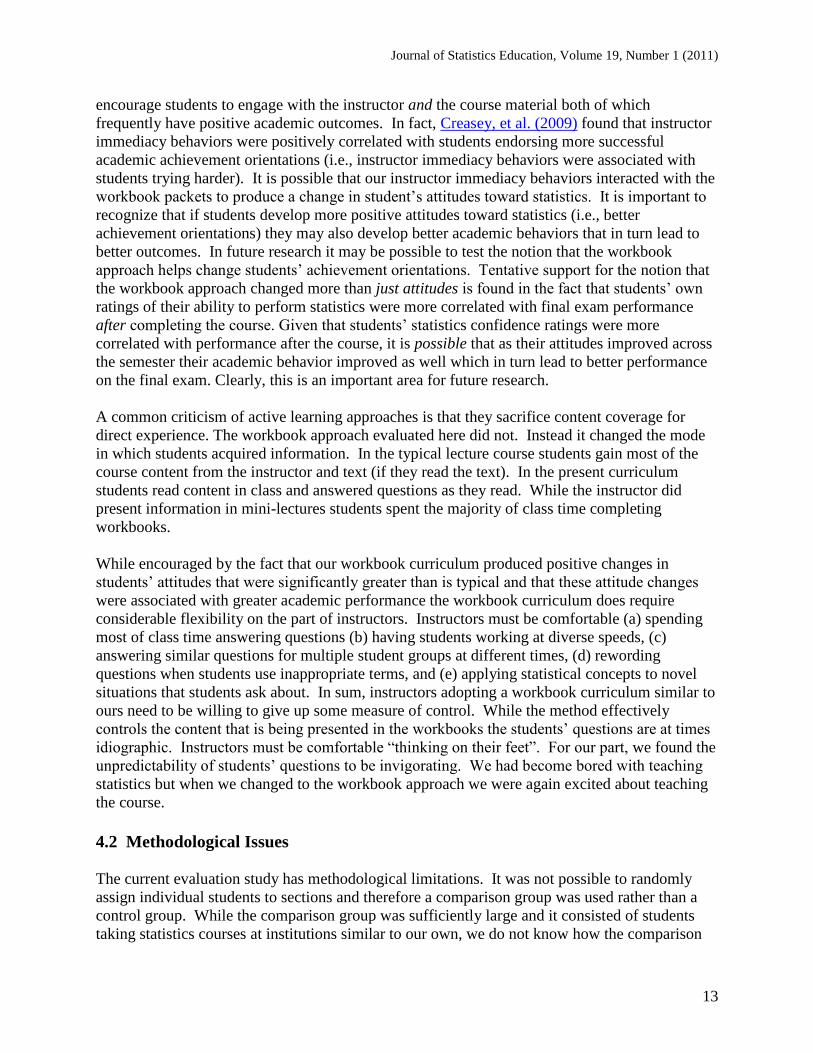
encourage students to engage with the instructor and the course material both of which

frequently have positive academic outcomes. In fact, Creasey, et al. (2009) found that instructor

immediacy behaviors were positively correlated with students endorsing more successful

academic achievement orientations (i.e., instructor immediacy behaviors were associated with

students trying harder). It is possible that our instructor immediacy behaviors interacted with the

workbook packets to produce a change in student’s attitudes toward statistics. It is important to

recognize that if students develop more positive attitudes toward statistics (i.e., better

achievement orientations) they may also develop better academic behaviors that in turn lead to

better outcomes. In future research it may be possible to test the notion that the workbook

approach helps change students’ achievement orientations. Tentative support for the notion that

the workbook approach changed more than just attitudes is found in the fact that students’ own

ratings of their ability to perform statistics were more correlated with final exam performance

after completing the course. Given that students’ statistics confidence ratings were more

correlated with performance after the course, it is possible that as their attitudes improved across

the semester their academic behavior improved as well which in turn lead to better performance

on the final exam. Clearly, this is an important area for future research.

A common criticism of active learning approaches is that they sacrifice content coverage for

direct experience. The workbook approach evaluated here did not. Instead it changed the mode

in which students acquired information. In the typical lecture course students gain most of the

course content from the instructor and text (if they read the text). In the present curriculum

students read content in class and answered questions as they read. While the instructor did

present information in mini-lectures students spent the majority of class time completing

workbooks.

While encouraged by the fact that our workbook curriculum produced positive changes in

students’ attitudes that were significantly greater than is typical and that these attitude changes

were associated with greater academic performance the workbook curriculum does require

considerable flexibility on the part of instructors. Instructors must be comfortable (a) spending

most of class time answering questions (b) having students working at diverse speeds, (c)

answering similar questions for multiple student groups at different times, (d) rewording

questions when students use inappropriate terms, and (e) applying statistical concepts to novel

situations that students ask about. In sum, instructors adopting a workbook curriculum similar to

ours need to be willing to give up some measure of control. While the method effectively

controls the content that is being presented in the workbooks the students’ questions are at times

idiographic. Instructors must be comfortable “thinking on their feet”. For our part, we found the

unpredictability of students’ questions to be invigorating. We had become bored with teaching

statistics but when we changed to the workbook approach we were again excited about teaching

the course.

4.2 Methodological Issues

The current evaluation study has methodological limitations. It was not possible to randomly

assign individual students to sections and therefore a comparison group was used rather than a

control group. While the comparison group was sufficiently large and it consisted of students

taking statistics courses at institutions similar to our own, we do not know how the comparison


14

courses were structured and therefore we do not know to what degree these courses used active

learning or lecture approaches. It is possible that the effects in this study resulted from an

instructor effect (i.e., that both of us are such stellar instructors that any method we try would

lead to these results). While a possibility, we hasten to mention that we have tried many things

in our statistics classes that have not worked as well as the workbook approach evaluated here.

Additionally, the present evaluation is limited because it focused on students’ attitudes toward

statistics rather than directly comparing students’ actual performance. In classroom settings it is

difficult to directly compare students’ performance across courses because exams are frequently

very different. In the present study, we did not have access to the exams used in any of the 20

comparison sections. Therefore, a more direct comparison of our students’ statistical

performance relative to that of other students was not possible.

While assessing students’ actual performance seems the most obvious way to assess a

curriculum’s success, the reality is that comparing student performance across different

curriculums creates many methodological problems. For example, it is easiest to compare

students’ performance when alternative curricula (i.e., teaching methods) cover identical content.

However, to reliably measure what students have learned in a curriculum, instructors create

items that are specific to that curriculum. To the extent that two curricula differ the tests used to

assess each curriculum’s impact should differ. When instructors/researchers emphasize easy

curricula comparison by using a common test they often sacrifice some assessment accuracy.

Ironically, if the teaching methods being evaluated are quite different a common test may not be

a “fair” comparison. This was the case in this study. Our previous lecture course emphasized

computation more and conceptual understanding less than our workbook approach. This

difference in emphasis made comparing these two curricula via identical exams

methodologically problematic.

Another challenging aspect of evaluating curricula arises from instructor and student differences

across course sections. Even if the same instructor taught two sections of a course during the

same semester using an “old” curriculum in one section and a “new” curriculum in the other

wide differences in students’ GPAs across course sections could still make direct comparisons of

students’ performance across sections problematic. Even if instructors could statistically correct

for GPA it is possible that instructors expected their innovation to be beneficial and it was their

expectation that boosted students’ performance rather than the innovation. Alternatively, if an

experimental section did not perform better, it is possible that the instructors were less familiar

with the new curriculum which suppressed students’ performance. It is important to recognize

that even when researchers hold instructor and tests constant comparing students’ performance

across sections is problematic.

We are not trying to induce hopelessness in classroom researchers; rather our point is that direct

measures of students’ performance are not without their methodological limitations. While

researchers should do their best to obtain direct measures of students’ performance when

evaluating their curricular changes, using standardized measures of students’ attitudes can

provide researchers with a common metric with which to compare curricula. Given that direct

measures of performance are often difficult to interpret methodologically we argue that assessing

students’ attitudes can be valuable to classroom researchers. This argument is bolstered by the

fact that student attitude measures are often correlated with performance (Chiesi and Primi,


15

2009; Elmore, et al., 1993; Finney and Schraw, 2003; Roberts and Saxe, 1982; Schau, 2003;

Schutz, Drogosz, White, and Distefano, 1998; Sorge and Schau, 2002) and future enrollment

choices (Finney and Schraw, 2003).

In sum, there are times when instructors cannot compare students’ actual performance and/or

times when doing so is less than optimal. In these situations comparing students’ attitudes about

course material may provide a solution to the curriculum evaluation problem, namely, a useful

metric for assessing an individual curriculum’s impact as well as a common measure for

comparing the relative impacts of different curricula. In these situations student attitudes can be

used instead of, or in addition to, measures of students’ actual performance.

4.3 General Conclusion In conclusion, the present study found that students who experienced the workbook approach had

positive changes in their attitudes toward statistics. Further these positive changes were

positively correlated with both students’ final exam performance and their GPA. Collectively,

these results suggest that the workbook approach shows promise as an educational approach in

college statistics courses.


16

Appendix A

CHAPTER 7-1: DISTRIBUTION OF SAMPLE MEANS

LEARNING OBJECTIVES

After reading the chapter, completing the homework and this activity you should be able to do the following:

o Explain what a distribution of sample means is.

o Explain how a distribution of raw scores is different from a distribution of sample means

that is created from those raw scores.

o Find the mean and the standard deviation of a distribution of sample means.

o Explain what the standard error of the mean measures.

o Compute sampling error.

o Describe how the standard error of the mean can be decreased.

o Explain why you would want the standard error of the mean to be minimized.

THE DISTRIBUTION OF SAMPLE MEANS AND SAMPLING ERROR

1. Why are researchers frequently forced to work with samples when they are really interested in populations?

2. When researchers work with samples, there is always the risk of large amounts of sampling error (i.e., getting a sample the does not represent the population accurately). Why is sampling error a problem for researchers?

If a study has too much sampling error it is not useful to researchers. In your last activity you learned that increasing sample size decreases sampling error. In this activity you will learn why increasing sample size decreases sampling error. You must understand the distribution of sample means if you hope to understand more advanced topics presented later in this course. A distribution of sample means is defined as all possible random sample means of a given size (n) from a particular population. In this activity you are going to “build” a distribution of sample means and then use it to calculate the average amount of sampling error researchers should expect to have in their study. Working with a very small population is probably the easiest way to start. Thus, you are going to work with a population of just four people. Researchers are usually interested in much larger populations, but it is much easier to illustrate what a distribution of sample means is by working with a very small population. Suppose there is a very small population of 4 billionaires who live in Norway. Further suppose that the data below represents the number of years of college/grad school each billionaire completed:


17

2, 4, 6, 8 (*note--this data is completely made up) 3. What is the mean for this population? µ = _______

4. What is the standard deviation for this population? σ = ________

Because there is just one of each score, the frequency distribution bar graph would be quite simple:

To create a distribution of sample means we need to obtain ALL possible RANDOM samples of a given size from this population. For this example, we are going to use a sample size of n = 2. Because the samples must be random we must be sure to sample with replacement. Thus, you would choose one score at random, put it back in the population, and then choose again at random. All possible random samples with n = 2 are listed below. The 16 samples below are ALL of the possible combinations of two scores from the population of 4 billionaires in Norway. Some of these samples represent the population much better than other samples. Which sample means represent the population well and which sample means do not? To answer this question compute the mean years of education for each of the 16 samples. Then determine which samples represent the population well and which do not.

5. Complete the table by finding the mean for each sample.

Sample First Score Second Score Mean

1 2 2

2 2 4

3 2 6

4 2 8

5 4 2

6 4 4

7 4 6

8 4 8

9 6 2

10 6 4

11 6 6

12 6 8

13 8 2

14 8 4

15 8 6

16 8 8

0

1

2

3

1 2 3 4 5 6 7 8

freq

uen

cy

Years of Education


18

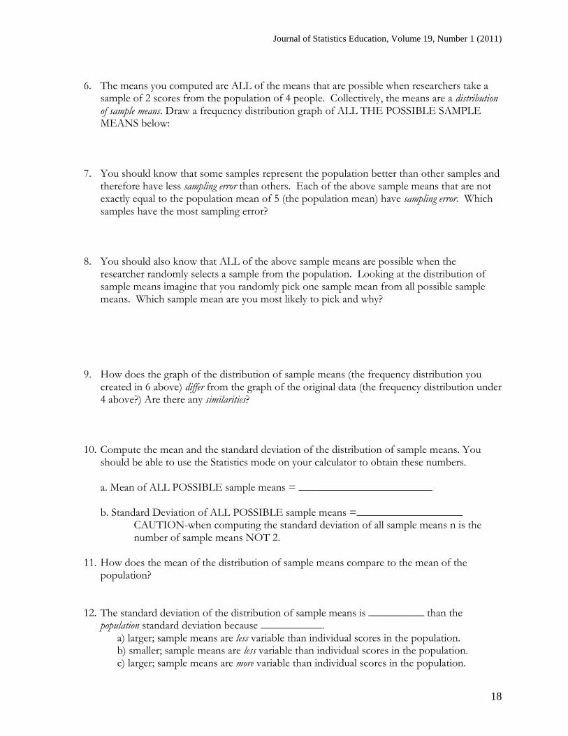
6. The means you computed are ALL of the means that are possible when researchers take a

sample of 2 scores from the population of 4 people. Collectively, the means are a distribution of sample means. Draw a frequency distribution graph of ALL THE POSSIBLE SAMPLE MEANS below:

7. You should know that some samples represent the population better than other samples and therefore have less sampling error than others. Each of the above sample means that are not exactly equal to the population mean of 5 (the population mean) have sampling error. Which samples have the most sampling error?

8. You should also know that ALL of the above sample means are possible when the researcher randomly selects a sample from the population. Looking at the distribution of sample means imagine that you randomly pick one sample mean from all possible sample means. Which sample mean are you most likely to pick and why?

9. How does the graph of the distribution of sample means (the frequency distribution you created in 6 above) differ from the graph of the original data (the frequency distribution under 4 above?) Are there any similarities?

10. Compute the mean and the standard deviation of the distribution of sample means. You should be able to use the Statistics mode on your calculator to obtain these numbers.

a. Mean of ALL POSSIBLE sample means = ________________________ b. Standard Deviation of ALL POSSIBLE sample means =___________________

CAUTION-when computing the standard deviation of all sample means n is the number of sample means NOT 2.

11. How does the mean of the distribution of sample means compare to the mean of the

population? 12. The standard deviation of the distribution of sample means is __________ than the

population standard deviation because ___________. a) larger; sample means are less variable than individual scores in the population. b) smaller; sample means are less variable than individual scores in the population. c) larger; sample means are more variable than individual scores in the population.


19

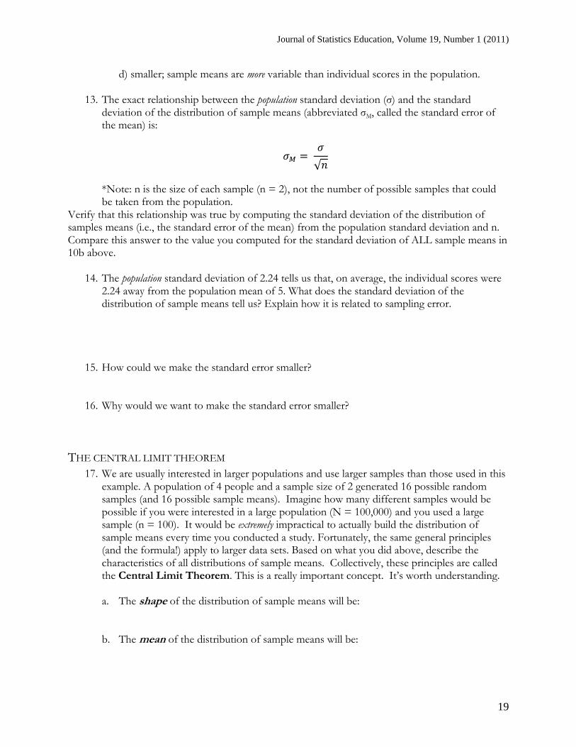
d) smaller; sample means are more variable than individual scores in the population.

13. The exact relationship between the population standard deviation (σ) and the standard deviation of the distribution of sample means (abbreviated σM, called the standard error of the mean) is:

*Note: n is the size of each sample (n = 2), not the number of possible samples that could be taken from the population.

Verify that this relationship was true by computing the standard deviation of the distribution of samples means (i.e., the standard error of the mean) from the population standard deviation and n. Compare this answer to the value you computed for the standard deviation of ALL sample means in 10b above.

14. The population standard deviation of 2.24 tells us that, on average, the individual scores were 2.24 away from the population mean of 5. What does the standard deviation of the distribution of sample means tell us? Explain how it is related to sampling error.

15. How could we make the standard error smaller? 16. Why would we want to make the standard error smaller?

THE CENTRAL LIMIT THEOREM

17. We are usually interested in larger populations and use larger samples than those used in this example. A population of 4 people and a sample size of 2 generated 16 possible random samples (and 16 possible sample means). Imagine how many different samples would be possible if you were interested in a large population (N = 100,000) and you used a large sample (n = 100). It would be extremely impractical to actually build the distribution of sample means every time you conducted a study. Fortunately, the same general principles (and the formula!) apply to larger data sets. Based on what you did above, describe the characteristics of all distributions of sample means. Collectively, these principles are called the Central Limit Theorem. This is a really important concept. It’s worth understanding.

a. The shape of the distribution of sample means will be:

b. The mean of the distribution of sample means will be:


20

c. The standard deviation of the distribution of sample means will be:

18. Explain how you can use the Central Limit Theorem to compute the expected amount of sampling error in a given study before the study is conducted.

Note: The basis of this activity (i.e., generating an entire distribution of sample means from a population of four numbers) was adapted from Gravetter and Wallnau (2007).

Acknowledgement

We are indebted to Candance Schau and Margorie Bond for providing us with normative SATS

data.

References

Bates Prins, S. C. (2009), “Student-Centered Instruction In A Theoretical Statistics Course,”

Journal of Statistics Education, 13(3).

http://www.amstat.org/publications/jse/v17n3/batesprins.html

Cashin, S. E., and Elmore, P. B. (2005), “The Survey of Attitudes Toward Statistics scale: A

construct validity study,” Educational and Psychological Measurement, 65(3), 509-524.

Chiesi, F. and Primi, C. (2009), “Assessing statistics attitudes among college students:

Psychometric properties of the Italian version of the Survey of Attitudes toward Statistics

(SATS),” Learning and Individual Differences, 2, 309-313.

Christopher, A. and Marek, P. (2009), “A palatable introduction to and demonstration of

statistical main effects and interactions,” Teaching of Psychology, 36(2), 130-133.

Creasey, G., Jarvis, P. and Gadke, D. (2009), “Student attachment stances, instructor immediacy,

and student-instructor relationships as predictors of achievement expectancies in college

students,” Journal of College Student Development, 50(4), 353-372.

http://www.amstat.org/publications/jse/v17n3/batesprins.html


21

DeVaney, T. A. (2010), “Anxiety and Attitude of Graduate Students in On-Campus vs. Online

Statistics Courses,” Journal of Statistics Education, 18(1).

http://www.amstat.org/publications/jse/v18n1/devaney.pdf

Elmore, P. B., Lewis, E. L., and Bay, M. L. G. (1993), "Statistics achievement: A function of

attitudes and related experience," Paper presented at the annual meeting of the American

Educational Research Association, Atlanta, GA.

Field, A. (2009), Discovering Statistics Using SPSS (3rd

ed.), London: Sage Publications Ltd.

Finney, S. J., & Schraw, G. (2003), “Self-efficacy beliefs in college statistics courses,”

Contemporary Educational Psychology, 28, 161-186.

Harlow, L. L., Burkholder, G. J., and Morrow, J. A. (2002), “Evaluating attitudes, skill, and

performance in a learning-enchanced quantitative methods course: A structural modeling

approach,” Structural Equation Modeling, 9, 413-430.

Hilton, S., Schau, C., and Olsen, J. (2004), “Survey of Attitudes Toward Statistics: Factor

structure invariance by gender and by administration time,” Structural Equation Modeling, 11(1),

92-109.

Knypstra, S. (2009), “Teaching Statistics in an Activity Encouraging Format,” Journal of

Statistics Education, 17(2). http://www.amstat.org/publications/jse/v17n2/knypstra.html

Manning, K., Zachar, P., Ray, G., and LoBello, S. (2006), “Research methods courses and the

scientist and practitioner interests of psychology majors,” Teaching of Psychology, 33(3), 194-

196.

Mottet, T. P., Parker-Raley, J., Beebe, S. A., Cunningham, C. (2007). “Instructors who resist

“College Lite”: The neutralizing effect of instructor immediacy on students’ course-workload

violations and perceptions of instructor credibility and affective learning,” Communication

Education, 56(2), 145-167.

Page, M. (1990), “Active learning: Historical and contemporary perspectives,” unpublished Ph.

D. dissertation, University of Massachusetts, Dept of Education.

Pfaff, T. P., and Weinberg, A. (2009), “Do hands-on activities increase student understanding?:

A case study,” Journal of Statistics Education, 17(3).

http://www.amstat.org/publications/jse/v17n3/pfaff.html

Roberts, D., and Saxe, J. (1982), “Validity of a statistics attitude survey: A follow-up study,”

Educational and Psychological Measurement, 42(3), 907-912.

Ryan, R. S. (2006), “A hands-on exercise improves understanding of the standard error of the

mean,” Teaching of Psychology, 33(3), 180-183.

http://www.amstat.org/publications/jse/v18n1/devaney.pdf

http://www.amstat.org/publications/jse/v17n2/knypstra.html

http://www.amstat.org/publications/jse/v17n3/pfaff.html


22

Sizemore, O. J. and Lewandowski, G W. (2009), “Learning might not equal liking: Research

methods course changes knowledge but not attitudes.,” Teaching of Psychology, 36(2), 90-95.

Schau, C. (2003, August). Students' attitudes: The "other" important outcome in statistics

education. Joint Statistical Meetings, San Francisco, CA.

Schau, C., Stevens, J., Dauphinee, T. L., and Del Vecchio, A. (1995), “The development and

validation of the Survey of Attitudes Toward Statistics,” Educational and Psychological

Measurement. 55, 868-875.

Schutz, P., Drogosz, L., White, V., and DiStefano, C. (1998), “Prior knowledge, attitude, and

strategy use in an introduction to statistics course,” Learning and Individual Differences, 10(4),

291-308.

Sorge, C., and Schau, C. (2002, April). Impact of engineering students' attitudes on achievement

in statistics. American Educational Research Association, New Orleans, AERA 2002.

Steinhorst, R. K. and Keeler, C. M. (1995), “Using Small Groups to Promote Active Learning in

the Introductory Statistics Course: A Report from the Field,” Journal of Statistics Education,

3(2). http://www.amstat.org/publications/jse/v3n3/steinhorst.html

Weltman, D. and Whiteside, M. (2010), "Comparing the Effectiveness of Traditional and Active

Learning Methods in Business Statistics: Convergence to the Mean," Journal of Statistics

Education [Online], 18(1), www.amstat.org/publications/jse/v18n1/weltman.pdf

Yoder, J., and Hochevar, C. (2005), “Encouraging active learning can improve students’

performance on examinations.” Teaching of Psychology, 32(2), 91-95.

Kieth A. Carlson


1001 Campus Drive

Valparaiso, IN 46383

[email protected]

(219) 464-5442

Jennifer Winquist


1001 Campus Drive

Valparaiso, IN 46383

[email protected]

(219) 464-5841

http://evaluationandstatistics.com/AERA2002.pdf

http://www.amstat.org/publications/jse/v3n3/steinhorst.html

http://www.amstat.org/publications/jse/v18n1/weltman.pdf

mailto:[email protected]



23

Volume 19 (2011) | Archive | Index | Data Archive | Resources | Editorial Board |

Guidelines for Authors | Guidelines for Data Contributors | Guidelines for Readers/Data Users | Home Page | Contact JSE | ASA Publications

http://www.amstat.org/publications/jse/contents_2011.htm

http://www.amstat.org/publications/jse/jse_archive.htm

http://www.amstat.org/publications/jse/jse_index.htm

http://www.amstat.org/publications/jse/jse_data_archive.htm

http://www.amstat.org/publications/jse/jse_info_service.htm

http://www.amstat.org/publications/jse/jse_board.htm

http://www.amstat.org/publications/jse/jse_author_info.htm

http://www.amstat.org/publications/jse/jse_data_contributor_info.htm

http://www.amstat.org/publications/jse/jse_users.htm

http://www.amstat.org/publications/jse/jse_users.htm

http://www.amstat.org/publications/jse/


http://www.amstat.org/publications/

Documents

Evaluating an active learning approach to teaching introductory