Estimation of the Transition Probabilities in Multi-state

Estimation of the Transition Probabilities in Multi-state SurvivalData: New Developments and Practical Recommendations

GUSTAVO SOUTINHOEPIUnit

University of PortoRua das Taipas 135, 4050-600 Porto

PORTUGAL

LUIS MEIRA-MACHADOUniversity of Minho

Department of MathematicsCampus de Azurem - 4800-058 Guimaraes

PORTUGAL

Abstract: Multi-state models can be successfully used for describing complicated event history data, for example,describing stages in the disease progression of a patient. In these models one important goal is the estimation ofthe transition probabilities since they allow for long term prediction of the process. Traditionally these quantitieshave been estimated by the Aalen-Johansen estimator which is consistent if the process is Markovian. Recently,estimators have been proposed that outperform the Aalen-Johansen estimators in non-Markov situations. Thispaper considers a new proposal for the estimation of the transition probabilities in a multi-state system that is notnecessarily Markovian. The proposed product-limit nonparametric estimator is defined in the form of a countingprocess, counting the number of transitions between states and the risk sets for leaving each state with an inverseprobability of censoring weighted form. Advantages and limitations of the different methods and some practicalrecommendations are presented. We also introduce a graphical local test for the Markov assumption. Severalsimulation studies were conducted under different data scenarios. The proposed methods are illustrated with a realdata set on colon cancer.

Key–Words: Markov assumption, Multi-state models, Nonparametric estimation, Transition probabilities, SurvivalAnalysisReceived: January 4, 2020. Revised: May 11, 2020. Re-revised: June 2, 2020. Accepted: June 18, 2020. Published: July 2, 2020.

1 IntroductionMulti-state models ([1], [2], [3], [4]) are models for astochastic process, which at any time occupies one ofa set of discrete states. These models provide a rele-vant modeling framework to deal with complex longi-tudinal survival data in which individuals may experi-ence more than one single event type. In such survivalstudies, besides overall survival, more than one end-point can be observed making the use of multi-statemodels preferable over traditional survival methods(e.g., the Cox model and the Kaplan-Meier estimatorof survival). A wide range of biomedical situationshave been modeled using multi-state methods, for ex-ample, HIV infection and AIDS [5], liver cirrhosis [6],breast cancer ([7]; [8]) and problems following hearttransplantation [3]. The states are usually based onclinical symptoms (e.g., bleeding episodes), biolog-ical markers (CD4 T-lymphocyte cell counts, serumimmunoglobulin levels), some scale of the disease(e.g., stages of cancer or VIH infection) or a non-fatalcomplication in the course of the illness (e.g., hearttransplantation). In cancer studies, besides death otherendpoints such as locoregional recurrence and distantmetastasis are often observed. A change of state is

called a transition, or an event. States can be transientor absorbing. An absorbing state is a process to whichone will never leave once it enters.

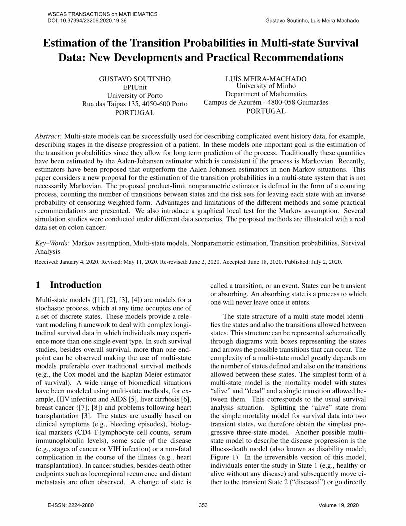
The state structure of a multi-state model identi-fies the states and also the transitions allowed betweenstates. This structure can be represented schematicallythrough diagrams with boxes representing the statesand arrows the possible transitions that can occur. Thecomplexity of a multi-state model greatly depends onthe number of states defined and also on the transitionsallowed between these states. The simplest form of amulti-state model is the mortality model with states“alive” and “dead” and a single transition allowed be-tween them. This corresponds to the usual survivalanalysis situation. Splitting the “alive” state fromthe simple mortality model for survival data into twotransient states, we therefore obtain the simplest pro-gressive three-state model. Another possible multi-state model to describe the disease progression is theillness-death model (also known as disability model;Figure 1). In the irreversible version of this model,individuals enter the study in State 1 (e.g., healthy oralive without any disease) and subsequently move ei-ther to the transient State 2 (“diseased”) or go directly

WSEAS TRANSACTIONS on MATHEMATICS DOI: 10.37394/23206.2020.19.36 Gustavo Soutinho, Luis Meira-Machado

E-ISSN: 2224-2880 353 Volume 19, 2020

to the absorbing “dead” state. Individuals in State 2will eventually move to the absorbing state withoutany possibility of recovery. Many time-to-event datasets from medical studies with multiple end points canbe reduced to this generic structure.

The multi-state process can be fully character-ized through its transition intensities or by its tran-sition probabilities. The transition intensities are theinstantaneous hazards for movement from one stateto another. These functions can used to obtain esti-mates of the mean sojourn time in a given state andto determine the number of individuals in differentstates at a certain moment. Covariates may be in-corporated in models through transition intensities toexplain differences among individuals in the courseof the illness. The transition probabilities representthe conditional probabilities that can be used to ob-tain predictions of the clinical prognosis of a patientat a certain point in his/her recovery or illness process.Various aspects of the model dynamics can be cap-tured by the transition probabilities. The usual non-parametric method to estimate the transition probabil-ity matrix for non-homogeneous Markov processes isthe Aalen-Johansen estimator [9]. Recently, [10] pro-pose a modification of the Aalen-Johansen estimatorin the illness-death model based on presmoothing. Al-though both approaches may be used to consistentlyestimate the occupation probabilities for non-Markovprocesses ([11], [12], [13]), in general they providebiased estimators for the transition probabilities if theprocess is not Markovian [14].

Substitute estimators for the Aalen-Johansen esti-mator for a non-Markov illness-death process withoutrecovery were introduced by [14]. They showed thatthe alternative estimators may behave more efficientlythan the Aalen-Johansen when the Markov assump-tion is strongly violated. Recently, [15] recovered theapproach by [14] and proposed a closely related non-Markov estimator too. Both proposals ([14] and [15])have the drawback of requiring the support of the cen-soring distribution to contain the support of the life-time distribution, otherwise they only report valid esti-mators for truncated transition probabilities. To over-come this problem this issue was recently revisitedby [16] and [17] who propose alternative estimatorsbased on subsampling (also known as landmarking)which does not require the censoring support condi-tion.

In this paper we revisit the topic of the nonpara-metric estimation of the transition probabilities, by in-troducing competing estimators in a multi-state sys-tem that is not necessarily Markovian and that over-comes the referred assumption on the censoring sup-port. The new set of estimators are constructed usingthe cumulative hazard of the total time given a first

time but where each observation has been weightedusing the information of the first duration. One of theproposed estimator is equivalent to the estimators re-cently proposed by [16]. To evaluate the performanceof all estimators, several simulation studies were con-ducted under different data scenarios. Based on theseresults recommendations are given as to which esti-mators to use. We also revisit the problem of checkingthe Markov assumption. However, unlike the usualtests, we are interested in a more reliable test whichis used for a particular transition probability. To thisend, we introduce a graphical test for the Markovassumption based on the discrepancies between thenew Markov-free estimators and the so-called Aalen-Johansen estimator (Markovian).

1. Healthy 2. Diseased

3. Dead

1. Healthy 2. Diseased

3. Dead

Figure 1: Illness-death model.

The organization of the paper is as follows. Theestimators are introduced in Section 2. The finite sam-ple performance of the proposed estimators for thetransition probabilities is investigated via simulationsin Section 3. In Section 4 we analyze data from acolon cancer study with the proposed methods. Mainconclusions and specific recommendations are givenin Section 5.

2 Nonparametric Estimators

2.1 Notation

A multi-state model is a stochastic process (Xt, t ∈T ) with a finite state space, where X(t) representsthe state occupied by the process at time t. In thispaper we consider the progressive illness-death modeldepicted in Figure 1 and we assume that all subjectsare in State 1 at time t = 0. Individuals may passfrom the healthy state (State 1), to the disease state(State 2) and then to the absorbing dead state (State 3).Individuals are at risk of death in each transient state(States 1 and 2). This means that one individual mayvisit State 2 or go directly to State 3 without visitingState 2.

Let Z denote the sojourn time in State 1, T thetotal survival time of the process and ρ = I(Z < T )the indicator of visiting State 2 at some time. For thismodel the transitions allowed are 1 → 2, 1 → 3 and


E-ISSN: 2224-2880 354 Volume 19, 2020

2 → 3. As usual with survival data, individuals aregenerally followed over a certain period of time, pro-viding right-censored observations. Let C denote theright-censoring variable, assumed to be independentof (Z, T ) (C⊥(Z, T )). Due to censoring, rather than(Z, T ) we observe (Z, T ,∆1,∆2) where Z = Z ∧ Cand T = T ∧ C are the censored versions of Z andT , and ∆1 = I(Z ≤ C) and ∆ = I(T ≤ C) therespective censoring indicators. Let{(

Zi, Ti,∆1i,∆i, ρi

), 1 ≤ i ≤ n

}be a random sample of the vector

(Z, T ,∆1,∆, ρ

).

For two states h, j and two time points s < t,introduce the so-called transition probabilities

phj(s, t) = P (X(t) = j|X(s) = h).

In the illness-death model we have five dif-ferent transition probabilities to estimate: p11(s, t),p12(s, t), p13(s, t), p22(s, t) and p23(s, t). Using theintroduced notation, the transition probabilities can bewritten as

p11(s, t) = P (Z > t | Z > s) ,

p12(s, t) = P (Z ≤ t, T > t | Z > s) ,

p13(s, t) = P (T ≤ t | Z > s) ,

p22(s, t) = P (Z ≤ t, T > t | Z ≤ s, T > s) ,

p23(s, t) = P (T ≤ t | Z ≤ s, T > s) .

from which it follows

p11(s, t) =P (Z > t)

P (Z > s),

p12(s, t) =P (s < Z ≤ t, T > t)

P (Z > s),

p13(s, t) =P (Z > s, T ≤ t)

P (Z > s),

p22(s, t) =P (Z ≤ s, T > t)

P (Z ≤ s, T > s),

p23(s, t) =P (Z ≤ s, s < T ≤ t)P (Z ≤ s, T > s)

.

Since we have two obvious relations p12(s, t) =1− p11(s, t)− p13(s, t) and p23(s, t) = 1− p22(s, t)this means that in practice we only need to estimatethree transition probabilities.

The inference in multi-state models is tradition-ally performed under the Markov assumption, whichstates that the relevant information for the future evo-lution of the process is provided by its current state,

independently of the states previously visited and thetransition times among them. Under this assumption,the transition probabilities can be estimated nonpara-metrically using Aalen-Johansen estimators [9]. Theirestimation method extends the time-honored Kaplan-Meier estimator to Markov chains. The Kaplan-Meierestimator is the standard method to estimate the sur-vival function from time-to-event data that are subjectto right censoring. It is a step function with jumps atevent times. The size of the steps depends on the num-ber of events and the number of individuals at riskat the corresponding time. Explicit formulae of theAalen-Johansen estimators (AJ) for the illness-deathmodel are available [18]. In the following sections weintroduce alternative non-Markov estimators for thesame target.

2.2 Kaplan-Meier weighted estimators

For a general non-Markov illness-death process with-out recovery, [14] derived estimators for the transitionprobabilities defined in terms of multivariate “Kaplan-Meier integrals” with respect to the marginal distribu-tion of the total time T . In particular, the estimatorsof p12(s, t) and p22(s, t) were proposed as an alterna-tive to the Aalen-Johansen estimators in non-Markovsituations. The transition probability p11(s, t) is de-fined as the ratio of observed survival distributions(and they can be estimated by the ordinary Kaplan-Meier estimator of survival [19] of the sojourn time inState 1, which we denote by S0). The denominator ofp12(s, t) can be estimated in the same way. The re-maining quantities involve expectations of particulartransformations of the pair (Z, T ),E [ϕ (Z, T )] whichcan not be estimated so simply

p LIDA12 (s, t) =

E(ϕs,t(Z, T ))

S0(s)(1)

and

p LIDA22 (s, t) =

E(ϕs,t(Z, T ))

E(ϕs,s(Z, T ))(2)

where ϕs,t(u, v) = I(s < u ≤ t, v > t) andϕs,t(u, v) = I(u ≤ s, v > t) and E(ϕs,t(Z, T )) isthe “Kaplan-Meier integral”

E(ϕs,t(Z, T )) =∑i

Wiϕs,t(Zi, Ti)

here Wi is the Kaplan-Meier weight attached to Tiwhen estimating the marginal distribution of T from


E-ISSN: 2224-2880 355 Volume 19, 2020

the(Ti,∆i

)’s (equal to minus the jump at Ti of the

Kaplan-Meier estimator of survival of the total timeS). See [14] for more details.

The methods proposed by [14] have the drawbackof requiring that the support of the censoring distribu-tion contains the support of the lifetime distribution.An assumption that is often not fulfilled in medical ap-plications due to limitations in the patient’s following-up. To avoid this potential problem, corrected estima-tors were proposed by [16] for p12(s, t) and p22(s, t):

pcLIDA12 (s, t) =S0(s)− S0(t)− E(γs,t(Z, T ))

S0(s)(3)

and

pcLIDA22 (s, t) = 1− E(γs,t(Z, T ))

S(t)− S0(s)(4)

where γs,t(u, v) = I(u > s, v ≤ t) and γs,t(u, v) =I(u ≤ s, s < v ≤ t).

All these quantities can be estimated nonparamet-rically using Kaplan-Meier weights.

2.3 Landmark Estimators

In this section we revisit the estimators proposed by[16] who propose alternative nonparametric estima-tors based on landmarking. The idea behind land-mark estimation is to use the information given by thestate occupied by the individual at a landmark timeprior to time t to estimate the conditional probabilitiespij(s, t) (being s the landmark time). In practice, non-parametric estimators for the transition probabilitiescan be introduced by considering specific subsamplesor portions of the data. In our case, to estimate thetransition probabilities p1j(s, t), for j = 1, 2, 3, theanalysis can be restricted to the individuals observedin State 1 at time s. As explained in [16], as long as Cis independent of Z, a subject in S1 =

{i : Zi > s

}is representative of those individuals for which Z ex-ceeds s. On the other hand, for the subpopulationZ > s, the censoring time C is still independent ofthe pair (Z, T ) and, therefore, Kaplan-Meier-basedestimation will be consistent. The same applies tothe analysis restricted to the individuals observed inState 2 at time s, say S2 =

{i : Zi ≤ s < Ti

}, which

serves to introduce landmark estimators for p2j(s, t),j = 2, 3. Accordingly, the following landmark esti-mators (LM) can be introduced,

pLM11 (s, t) = S(s)0 (t), (5)

pLM13 (s, t) = S(s)(t), (6)

where S(s)0 is the Kaplan-Meier estimator of survival

of the sojourn time in State 1 computed in the sub-sample S1; and S(s) is the Kaplan-Meier estimator ofsurvival of the total time computed in the same sub-sample. The formal relation p12(s, t) = 1−p11(s, t)−p13(s, t) can be used to estimate p12. Finally,

pLM23 (s, t) = S[s](t), (7)

where S[s] is the Kaplan-Meier estimator of survivalof the total time computed in the subsample S2.

It is worth mention that [17] also introduced anestimator based on subsampling which they termedas a landmark Aalen-Johansen estimator of the tran-sition probabilities. The idea behind the proposed es-timator is to use the Aalen-Johansen estimator of thestate occupation probabilities derived from those sub-sets (consisting of subjects occupying a given stateat a particular time). Simulation studies publishedin the paper by [17] show that the landmark Aalen-Johansen estimator (LMAJ) and the landmark estima-tor (LM) perform similarly. In fact, the two landmarkestimators (LM and LMAJ) of the transition probabili-ties p11(s, t), p22(s, t) and p23(s, t) are equivalent.

As a weakness, the landmark estimators [16] and[17] may provide large standard errors in estimation insome circumstances. This may occur for small sam-ple sizes and/or large proportion of censored data. Insuch cases the estimators based on a landmark ap-proach may result in a wiggly estimator with fewerjump points. A valid approach that can be used to re-duce the variability of these estimators is to consider amodification of the landmark estimator based on pres-moothing [20], [21].

2.4 Weighted Cumulative Hazard Estima-tors

In this section we propose new estimators for the tran-sition probabilities p11(s, t), p13(s, t) and p22(s, t).The estimators are constructed using the cumulativehazard of the total time given a first time but whereeach observation has been weighted using the infor-mation of the first duration. The proposed estimator(WCH - weighted cumulative hazard) for the transi-tion probability p11(s, t) is given by

p WCH11 (s, t) = P (Z > t | Z > s) ,

=∏v∈R1

{1− Λ11(dv)}, (8)


E-ISSN: 2224-2880 356 Volume 19, 2020

where Λ11(dv) is the cumulative conditional hazardof Z given Z > s. Assuming that Z⊥C, Λ11(dv) canbe estimated by

Λ11(dv) =

∑ni=1 I(Zi > s, Zi = v,∆1i = 1)∑n

i=1 I(Zi > s, Zi ≥ v)

and where R1 = {Zi : Zi ≤ t}.Estimator (8) is equivalent to the estimator pro-

posed by [14], [16] and the so-called Aalen-Johansenestimator [9].

Similar ideas can be used to obtain estimators forp13(s, t) and p22(s, t). Note that p13(s, t) = P (T ≤t | Z > s) = 1− P (T > t | Z > s). Then,

pWCH

13 (s, t) = 1− P (T > t | Z > s) ,

= 1−∏

v∈R13

{1− Λ13(dv)}∏

v∈R123

{1− Λ123(dv)}, (9)

where Λ13(dv) is the cumulative conditional hazardof T given Z > s for those individuals going directlyinto State 3 without visiting State 2; and Λ123(dv) isthe cumulative conditional hazard of T given Z > sfor those visiting State 2. Assuming that (Z, T )⊥C,Λ13(dv) can be estimated by

Λ13(dv) =

∑ni=1 I(Zi > s, Zi = Ti, Ti = v,∆2i = 1)∑n

i=1 I(Zi > s, Ti ≥ v)

and where R13 = {Ti : Ti ≤ t}; whereas Λ123(dv)can be estimated by

Λ123(dv) =

∑ni=1 I(Zi > s, Zi < Ti, Ti = v,∆2i = 1)∑n

i=1 I(Zi > s, Ti ≥ v)

and where R123 = {Ti : Ti ≤ t}.Then, p12(s, t) can be estimated by p WCH

12 (s, t) =1− p WCH

11 (s, t)− p WCH13 (s, t). Note that estimators of

p WCH1j (s, t) , j = 1, 2 are equivalent to the landmark

estimators proposed by [16].

Since p22(s, t) = P (Z<s,T>t)P (Z<s,T>s) = P (T>t|Z<s)

P (T>s|Z<s) .The key to estimating p22(s, t) is to estimate P (T >u | Z < s) for u ∈ {s, t}. These quantities can beestimated by

P (T > u | Z < s) =∏

v∈R23

{1− Λ23(dv)},(10)

where R23 = {T23i : T23i ≤ u − Zi, Zi < Ti}; andΛ23(dv) can be estimated by

Λ23(∆v) =

∑ni=1 I(Zi ≤ s, Zi < Ti, T23i = v,∆2i = 1)/G(Zi + v)∑ni=1 I(Zi ≤ s, Zi < Ti, T23i ≥ v,∆1i = 1)/G(Zi + v)

.

The resultant estimator is labeled as pWCH22 (s, t).Since p22(s, t) = P (T > t|Z < s, T > s), an

alternative estimator is given by

pWCH22 (s, t) = P (T > u | Z < s, T > s) =

∏v∈R?

23

{1− Λ?23(dv)}, (11)

where R?23 = {Ti : Ti ≤ t} and where Λ?

23(dv) canbe estimated by

Λ?23(∆v) =

∑ni=1 I(Zi ≤ s, Ti > s, Ti = v,∆2i = 1)/G(v)∑n

i=1 I(Zi ≤ s, Ti > s, Ti ≥ v,∆1i = 1)/G(max(Zi, v)).

The estimator pWCH22 (s, t) is equivalent to the land-mark estimator pLM22 (s, t) proposed by [16].

The estimation of the variance is important forinference purposes. Resampling techniques such asthe bootstrap provides here a practical solution to theproblem of variance estimation and inference. Thesemethods can be used to construct confidence limitsbased on the percentile bootstrap.

3 Simulation Study

In this section we investigate the performance ofthe proposed estimators through simulations. Morespecifically, the estimators introduced in Section 2 areconsidered. In particular we aim to compare the per-formance of the Aalen-Johansen estimator which ben-efits from the assumption of Markovianity on the un-derlying stochastic process, with alternative estima-tors which are free of the Markov condition. The sim-ulation addresses also the question about the more ef-ficient estimator in different scenarios.

To simulate the data in the irreversible illness-death model, we separately consider the subjects pass-ing through State 2 at some time (that is, those caseswith ρ = 1), and those who directly go to the absorb-ing State 3 (ρ = 0). For the second subgroup of indi-viduals (ρ = 0), times to death without illness are gen-erated from the hazard function h13(t) = 0.024 × t.For the first subgroup of individuals (ρ = 1), thesuccessive gap times (Z, T − Z) are simulated us-ing two cause-specific hazard functions, h12 and h23for each of the events (illness and death). The cause-specific hazard for the intermediate event was definedas h12(t) = 0.29

t+1 . For the individuals that experiencedthe disease, times to death after the disease were gen-erated using three different hazards:


E-ISSN: 2224-2880 357 Volume 19, 2020

h123(t, t12) = 0.05

h223(t, t12) =1

0.25(t12 + 1)0.8

h323(t, t12) = 0.04× log(t+ 1)

where t > 0, denotes the time since the start point,and t12 is the transition time from State 1 to State 2.

The use of these three different hazard functionsprovides three different scenarios. The first scenariocan be considered Markovian since the hazard ofdeath after the disease was set constant being indepen-dent of t and t12. In the two remaining scenarios, thehazard for death after disease depended on the thesetimes. The second scenario is semi-Markovian sincethe process depend not only the current state, but alsohow long it has been in the current state (time refers totime since entering the intermediate state). The thirdscenario is non-Markov since the hazard for death af-ter disease depended on the time since entry in study.

An independent uniform censoring timeC is gen-erated, according to models U [0, 40] and U [0, 30].For the Markovian scenario, the first model, presents19% of censoring on the first gap time Z, 40% cen-soring on the total time T and 42% on the secondgap time T − Z, for those individuals who enteredin state 2. The second model changes these censor-ing levels to 33%, 58% and about 36%, respectively.The first model in the semi-Markovian scenario, re-veals 23% of censoring for Z, 40% for T and 41%for T − Z. Second model increases these censoringlevels to 36%, 49% and 41%, respectively. Finally, inthe non-Markovian scenario, the model U [0, 40] pro-vides 25% of censoring on the first gap time, 43% onthe total time and 41% on the second gap time. Underthe model U [0, 30] censoring increases to 26%, 44%and about 42%, respectively.

For each simulated scenario we consider severaldifferent points (s, t) pairs, corresponding to combi-nations of times 2, 4, 8 and 12 representing the differ-ences between closer and distant times. Sample sizesn = 100 and n = 250 are considered. In each simula-tion, 1000 samples are generated. From these sampleswe obtained the mean for all generated data sets. Asa measure of efficiency, we took the Mean SquaredError (MSE) but we also computed the standard devi-ations (SD) and the Bias.

Tables 1 (Markov scenario), 2 (semi-Markov sce-nario) and 3 (non-Markov scenario) report the resultsfor transition probability p13(s, t). When one is confi-dent of the Markov assumption, the Aalen-Johansenis preferred over non-Markovian estimators since it

reports a smaller variance in estimation. This is in

agreeing with results reported in Table 1. Results re-ported in the Tables 2 and 3 also reveal that the Aalen-Johansen estimator (labeled as AJ) might still perform

reasonably well in situations where the process showsonly mild deviations from Markovianity. However,when there is strong evidence that the process is notMarkov the use of a non-Markov estimator is prefer-able due to their greater accuracy. This can be ob-served from results reported in Tables 2 and 3.

All three simulation scenarios reveal that the per-formance of the methods is poorer at the right tail.This was expected because for larger values of s and t,the censoring effects are stronger. The SD decreaseswith an increase of the sample size and with the de-crease of the censoring percentage, which was alsoexpected.

Results in Tables 1, 2 and 3 reveal a poor perfor-mance of the original non-Markov estimators by [14],referred to as LIDA estimators. The two methods al-ternative non-Markov methods (the corrected LIDA,labeled as cLIDA, and the Weighted Cumulative Haz-ard method WCH) obtain in all settings a negligiblebias (decreasing as the sample size increases), whilethe LIDA estimator show a systematic bias.

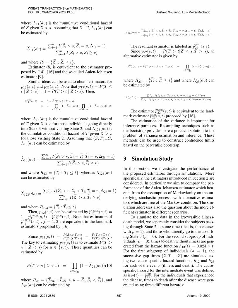
Tables 2 and 3 show that the Markov-free esti-mators cLIDA and WCH may behave much more ef-ficiently than the Aalen-Johansen. This is because ofthe failure of the Markov assumption from which theAalen-Johansen estimator is built. This is more ev-ident in the semi-Markov scenario, with higher lagtimes t − s. In these cases, the Aalen-Johansen showa systematic bias which does not decrease with an in-creasing sample size. In these cases the applicationof the Aalen-Johansen method is not recommendedhere, due to possible biases. The poor behavior of theAalen-Johansen estimator can also be seen in Figure2, in which we show the boxplots of the estimates ofthe transition probabilities based on the 1000 MonteCarlo replicates for the four estimators, with differentsample sizes. From these plots it can be seen that thecLIDA and WCHmethods are unbiased estimators andconfirm the less variability of the Aalen-Johansen es-timator. The WCH method (which in this case is equiv-alent to the LM method) is the preferred since is theunbiased method reporting less variability.

Tables 4, 5 and 6 report the results for five differ-ent estimators for the transition probability p22(s, t).Results reported in Table 4 reveal that the Aalen-Johansen estimator is the preferred since it reports un-biased estimates with smaller variance in estimation.This was expected since the process is Markovian inthis scenario. Again, it is important mentioning thatthis estimator which assumes the process to be Marko-vian still perform reasonably well in situations where


E-ISSN: 2224-2880 358 Volume 19, 2020

Tabl

e1:

Bia

san

dst

anda

rdde

viat

ion

(SD

)for

the

thre

ees

timat

ors

ofp13(s,t

).M

arko

vsc

enar

iow

ithtw

osa

mpl

esi

zes

and

two

cens

orin

gle

vels

.pAJ

13(s

,t)

pLIDA

13

(s,t)

pcLIDA

13

(s,t)

pWCH

13

(s,t)

bias

SDbi

asSD

bias

SDbi

asSD

(s,t)

=(2

,4)

n=10

0C∼

U[0,30]

<0.

0001

0029

90.

0345

0.05

33<

0.00

010.

0316

<0.

0001

0.03

16C∼

U[0,20]

<0.

0001

0.03

000.

0600

0.05

52<

0.00

010.

0312

<0.

0001

0.03

11n=

250

C∼

U[0,30]

<0.

0001

0.01

870.

0335

0.03

68<

0.00

010.

0197

<0.

0001

0.01

97C∼

U[0,20]

<0.

0001

0.01

930.

0584

0.03

83<

0.00

010.

0204

<0.

0001

0.02

04(s

,t)=

(2,8

)n=

100

C∼

U[0,30]

0.00

240.

0527

0.06

590.

0926

0.00

210.

0567

0.00

250.

0563

C∼

U[0,20]

0.00

140.

0594

0.11

80.

0907

0.00

100.

0630

<0.

0001

0.06

27n=

250

C∼

U[0,30]

<0.

0001

0.03

400.

0677

0.06

26<

0.00

010.

0363

<0.

0001

0.03

6C∼

U[0,20]

<0.

0001

0.03

750.

1147

0.06

07<

0.00

010.

0406

<0.

0001

0.04

01(s

,t)=

(4,1

2)n=

100

C∼

U[0,30]

-0.0

039

0.07

360.

0669

0.10

34-0

.002

90.

0791

-0.0

038

0.07

67C∼

U[0,20]

-0.0

024

0.08

240.

1084

0.11

81-0

.001

30.

0911

-0.0

014

0.08

93n=

250

C∼

U[0,30]

0.00

110.

0462

0.06

710.

0733

0.00

180.

0508

0.00

170.

0496

C∼

U[0,20]

<0.

0001

0.05

030.

1132

0.07

08<

0.00

010.

0541

<0.

0001

0.05

33(s

,t)=

(8,1

2)n=

100

C∼

U[0,30]

-0.0

015

0.08

160.

0424

0.10

3-0

.003

10.

0844

-0.0

029

0.08

39C∼

U[0,20]

-0.0

019

0.09

90.

0645

0.11

7-0

.001

60.

1034

-0.0

027

0.10

12n=

250

C∼

U[0,30]

<0.

0001

0.05

290.

0412

0.06

58<

0.00

010.

0551

<0.

0001

0.05

46C∼

U[0,20]

<0.

0001

0.06

210.

0615

0.07

85<

0.00

010.

0652

<0.

0001

.0.

0639

Tabl

e2:

Bia

san

dst

anda

rdde

viat

ion

(SD

)for

the

thre

ees

timat

ors

ofp13(s,t

).Se

mi-

Mar

kov

scen

ario

with

two

sam

ple

size

san

dtw

oce

nsor

ing

leve

ls.

pAJ

13(s

,t)

pLIDA

13

(s,t)

pcLIDA

13

(s,t)

pWCH

13

(s,t)

bias

SDbi

asSD

bias

SDbi

asSD

(s,t)

=(2

,4)

n=10

0C∼

U[0,30]

0.00

850.

0312

0.01

810.

0488

0.00

150.

0323

0.00

160.

0323

C∼

U[0,20]

0.00

570.

0311

0.03

330.

0534

<0.

0001

0.03

31<

0.00

010.

0331

n=25

0C∼

U[0,30]

0.00

710.

0197

0.01

580.

0337

<0.

0001

0.02

02<

0.00

010.

0202

C∼

U[0,20]

0.00

650.

0201

0.03

330.

0378

<0.

0001

0.02

08<

0.00

010.

0208

(s,t)

=(2

,8)

n=10

0C∼

U[0,30]

0.02

730.

0579

0.04

980.

087

0.00

140.

0617

0.00

140.

0610

C∼

U[0,20]

0.02

540.

0596

0.08

630.

0932

<0.

0001

0.06

39<

0.00

010.

0634

n=25

0C∼

U[0,30]

0.02

760.

0353

0.04

740.

0590

0.00

190.

0369

0.00

220.

0370

C∼

U[0,20]

0.02

570.

0354

0.08

400.

0629

<0.

0001

0.03

83<

0.00

010.

0378

(s,t)

=(4

,12)

n=10

0C∼

U[0,30]

0.03

280.

0757

0.07

610.

1059

0.00

350.

0798

0.00

350.

0783

C∼

U[0,20]

0.03

080.

0841

0.11

930.

1079

0,00

280.

0902

0.00

220.

0883

n=25

0C∼

U[0,30]

0.02

700.

0459

0.06

720.

0727

-0.0

024

0.04

98-0

.002

40.

0486

C∼

U[0,20]

0.02

710.

0530

0.11

060.

0744

-0.0

027

0.05

73-0

.002

00.

0562

(s,t)

=(8

,12)

n=10

0C∼

U[0,30]

0.00

850.

0842

0.05

050.

1056

<0.

0001

0.08

72-0

.001

20.

0861

C∼

U[0,20]

0.00

770.

0987

0.07

380.

1216

0.00

130.

1040

-0.0

013

0.10

04n=

250

C∼

U[0,30]

0.00

950.

0530

0.05

080.

0673

<0.

0001

0.05

50<

0.00

010.

0542

C∼

U[0,20]

0.00

850.

0596

0.07

200.

0750

-0.0

010

0.06

20-0

.001

10.

0608


E-ISSN: 2224-2880 359 Volume 19, 2020

Tabl

e3:

Bia

san

dst

anda

rdde

viat

ion

(SD

)for

the

thre

ees

timat

ors

ofp13(s,t

).N

on-M

arko

vsc

enar

iow

ithth

ree

sam

ple

size

san

dtw

oce

nsor

ing

leve

ls.

pAJ

13(s

,t)

pLIDA

13

(s,t)

pcLIDA

13

(s,t)

pWCH

13

(s,t)

bias

SDbi

asSD

bias

SDbi

asSD

(s,t)

=(2

,4)

n=10

0C∼

U[0,30]

0.00

180.

0282

0.01

470.

0488

-0.0

019

0.02

86-0

.001

90.

0285

C∼

U[0,20]

0.00

350.

0318

0.03

760.

0563

<0.

0001

0.03

25<

0.00

010.

0325

n=25

0C∼

U[0,30]

0.00

340.

0185

0.01

230.

0345

<0.

0001

0.01

88<

0.00

010.

0188

C∼

U[0,20]

0.00

300.

0191

0.03

090.

0413

<0.

0001

0.01

94<

0.00

010.

0194

(s,t)

=(2

,8)

n=10

0C∼

U[0,30]

0.01

310.

0563

0.02

520.

0936

-0.0

017

0.05

88-0

.001

40.

0586

C∼

U[0,20]

0.01

190.

0567

0.07

920.

0925

<0.

0001

0.06

03<

0.00

010.

0596

n=25

0C∼

U[0,30]

0.01

640.

0349

0.02

570.

0584

0.00

270.

0367

0.00

280.

0364

C∼

U[0,20]

0.01

400.

0365

0.06

860.

0711

<0.

0001

0.03

92<

0.00

010.

0390

(s,t)

=(4

,12)

n=10

0C∼

U[0,30]

0.01

760.

0749

0.03

160.

1103

<0.

0001

0.08

01-0

.001

50.

0786

C∼

U[0,20]

0.02

120.

0832

0.09

000.

1197

0.00

450.

0906

0.00

340.

0869

n=25

0C∼

U[0,30]

0.02

040.

0468

0.02

400.

0783

<0.

0001

0.05

06<

0.00

010.

0498

C∼

U[0,20]

0.01

790.

0527

0.08

150.

0841

-0.0

017

0.05

83-0

.001

50.

0567

(s,t)

=(8

,12)

n=10

0C∼

U[0,30]

0.01

450.

0814

0.02

590.

1077

0.00

390.

0842

0.00

380.

0835

C∼

U[0,20]

0.00

600.

1005

0.06

100.

1246

-0.0

038

0.10

32-0

.003

40.

1031

n=25

0C∼

U[0,30]

0.00

870.

0527

0.01

890.

0709

<0.

0001

0.05

41<

0.00

010.

0539

C∼

U[0,20]

0.01

140.

0619

0.05

960.

0815

0.00

160.

0645

0.00

170,

0636

●

●

●●

●

●

●

●●

●

●

●

●

●

●

●

●●

●

●

●

●

●●

●

●

●

●

●

●

●●●

●

●

●●

●

●●●●●

●

●●●●

●

●

●

●

●

●

●

●

●

●

●

●

●●

●

●●

●●

●

●

●

●●●

●

●●●

●

●

●

●

●

●

●

●

●

●

●

●

●

●

●

●

●

AJ LIDA cLIDA WCH AJ LIDA cLIDA WCH

0.0

0.1

0.2

0.3

0.4

0.5

0.6

p12(

2,12

)

n = 100 n = 250

Figure 2: Boxplots of the M = 1000 estimates ofthe transition probabilities of the pAJ12 , pLIDA12 , pcLIDA12

and pWCH12 with two different samples sizes for semi-Markovian scenario. Censoring times were generatedfrom an uniform distribution on [0, 30].

the process shows only mild deviations from Marko-vianity. This occurs for example in the semi-Markovscenario with small lag times t − s. In these cases,the Aalen-Johansen reports estimates with small biasbut less variability and therefore low mean squarederrors. As the lag times t − s increase so the biasresulting in a clear biased estimator. This behavioris also present in the non-Markov scenario (Table 6).Results shown in Tables 5 and 6 reveals that whenthere is strong evidence that the process is not Markovthat the use of a non-Markov estimator is preferable.With the exception of the LIDA method all the re-maining non-Markov methods (cLIDA, LM and WCH)are valid alternative estimators due to their greater ac-curacy. Again, the performance of the LIDA methodis poorer even worst than the Aalen-Johansen estima-tor. Simulation results reveal that the LIDA estima-tor is systematically (downward) biased whereas thethree non-Markov methods cLIDA, LM and WCH areasymptotically unbiased. The best performance is at-tained by the non-Markov methods (cLIDA, LM andWCH) which lead to more efficient estimation of thetransition probabilities. This can be seen in all mea-sures (bias, standard deviation and mean square er-ror). However, when considering all scenarios andall pairs (s, t) neither of the two methods seems tobe uniformly best for estimating p22(s, t). However,


E-ISSN: 2224-2880 360 Volume 19, 2020

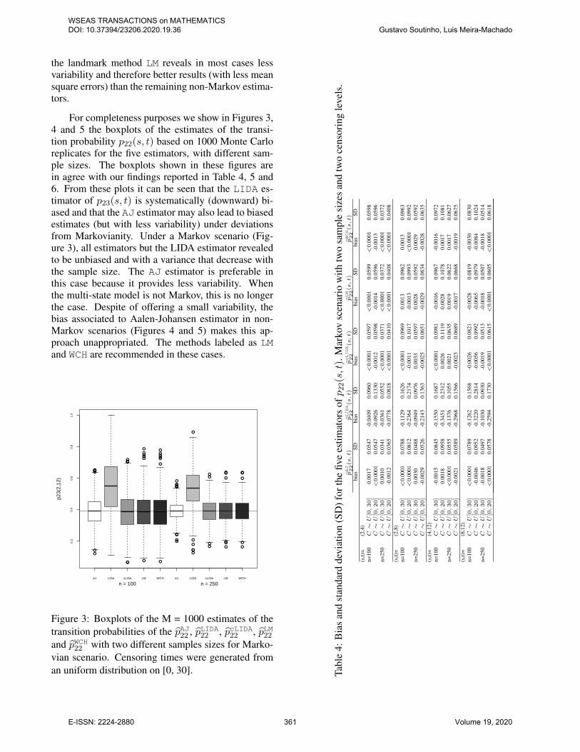
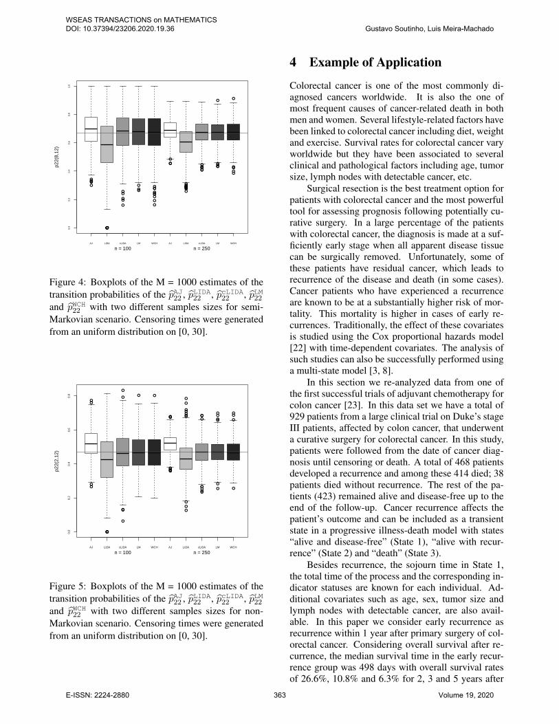
the landmark method LM reveals in most cases lessvariability and therefore better results (with less meansquare errors) than the remaining non-Markov estima-tors.

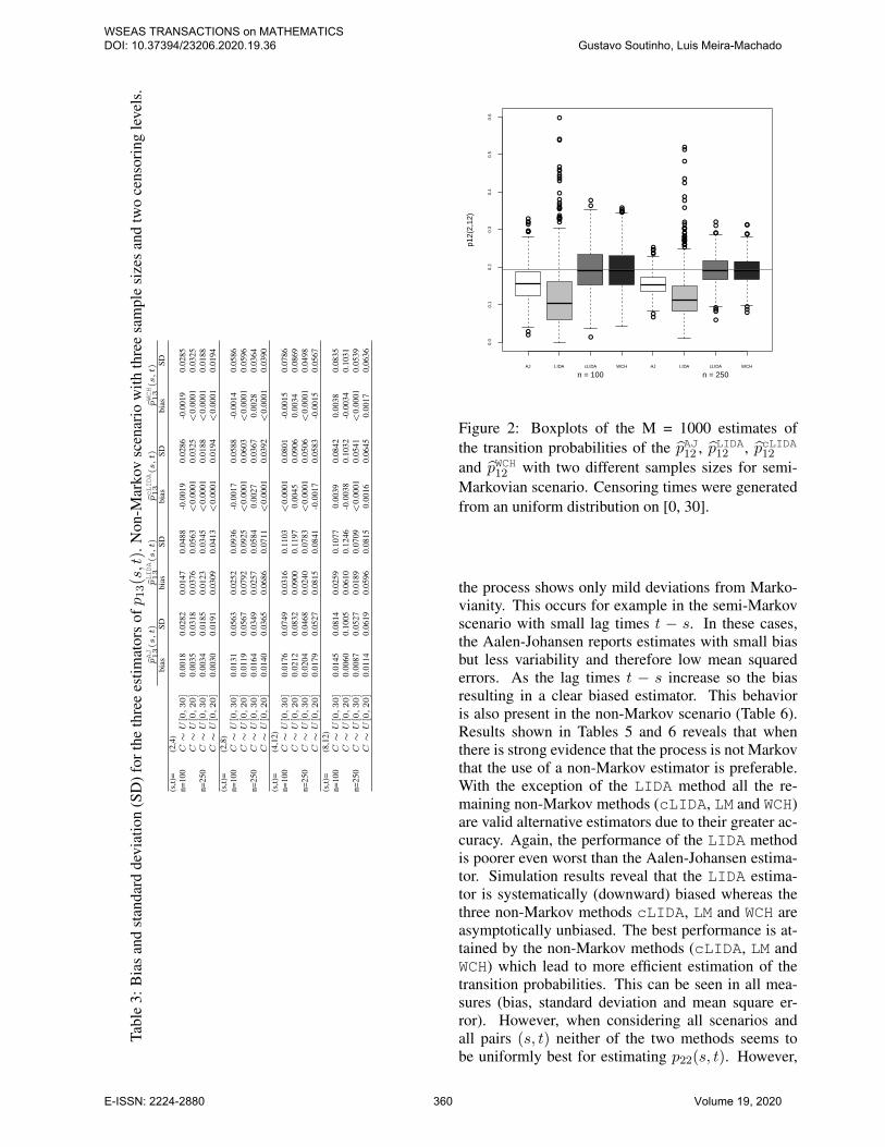
For completeness purposes we show in Figures 3,4 and 5 the boxplots of the estimates of the transi-tion probability p22(s, t) based on 1000 Monte Carloreplicates for the five estimators, with different sam-ple sizes. The boxplots shown in these figures arein agree with our findings reported in Table 4, 5 and6. From these plots it can be seen that the LIDA es-timator of p23(s, t) is systematically (downward) bi-ased and that the AJ estimator may also lead to biasedestimates (but with less variability) under deviationsfrom Markovianity. Under a Markov scenario (Fig-ure 3), all estimators but the LIDA estimator revealedto be unbiased and with a variance that decrease withthe sample size. The AJ estimator is preferable inthis case because it provides less variability. Whenthe multi-state model is not Markov, this is no longerthe case. Despite of offering a small variability, thebias associated to Aalen-Johansen estimator in non-Markov scenarios (Figures 4 and 5) makes this ap-proach unappropriated. The methods labeled as LMand WCH are recommended in these cases.

●●●●

●●

●

●●●

●

●

●

●

●●●

●

●

●

●●●

●

●

●

●

●

●

●

●●●●

●

●

●

●●

●

●

●

●

●●

● ●

●

●

●

●

● ●

●

●

●

●

AJ LIDA cLIDA LM WCH AJ LIDA cLIDA LM WCH

0.2

0.4

0.6

0.8

1.0

p23(

2,12

)

n = 100 n = 250

Figure 3: Boxplots of the M = 1000 estimates of thetransition probabilities of the pAJ22 , pLIDA22 , pcLIDA22 , pLM22and pWCH22 with two different samples sizes for Marko-vian scenario. Censoring times were generated froman uniform distribution on [0, 30]. Ta

ble

4:B

ias

and

stan

dard

devi

atio

n(S

D)f

orth

efiv

ees

timat

ors

ofp22(s,t

).M

arko

vsc

enar

iow

ithtw

osa

mpl

esi

zes

and

two

cens

orin

gle

vels

.pAJ

22(s

,t)

pLIDA

22

(s,t)

pcLIDA

22

(s,t)

pLM

22(s

,t)

pWCH

22

(s,t)

bias

SDbi

asSD

bias

SDbi

asSD

bias

SD(s

,t)=

(2,4

)n=

100

C∼

U[0,30]

0.00

170.

0547

-0.0

409

0.09

60<

0.00

010.

0597

<0.

0001

0.05

99<

0.00

010.

0598

C∼

U[0,20]

<0.

0001

0.05

47-0

.092

60.

1330

-0.0

012

0.05

98-0

.001

40.

0596

-0.0

013

0.05

96n=

250

C∼

U[0,30]

0.00

100.

0341

-0.0

361

0.05

52<

0.00

010.

0371

<0.

0001

0.03

72<

0.00

010.

0372

C∼

U[0,20]

-0.0

012

0.03

65-0

.077

80.

0818

<0.

0001

0.04

10<

0.00

010.

0408

<0.

0001

0.04

08(s

,t)=

(2,8

)n=

100

C∼

U[0,30]

<0.

0001

0.07

88-0

.112

90.

1626

<0.

0001

0.09

690.

0013

0.09

620.

0013

0.09

63C∼

U[0,20]

<0.

0001

0.08

12-0

.236

40.

2174

-0.0

011

0.10

17-0

.001

30.

0993

<0.

0001

0.09

92n=

250

C∼

U[0,30]

0.00

300.

0488

-0.0

949

0.09

760.

0033

0.05

970.

0028

0.05

920.

0029

0.05

92C∼

U[0,20]

-0.0

029

0.05

26-0

.214

30.

1363

-0.0

025

0.06

51-0

.002

90.

0634

-0.0

028

0.06

35(s

,t)=

(4,1

2)n=

100

C∼

U[0,30]

-0.0

015

0.08

45-0

.155

00.

1687

<0.

0001

0.09

81-0

.001

60.

0967

-0.0

016

0.09

72C∼

U[0,20]

0.00

180.

0958

-0.3

451

0.23

120.

0026

0.11

190.

0028

0.10

780.

0017

0.10

81n=

250

C∼

U[0,30]

<0.

0001

0.05

55-0

.137

60.

1055

0.00

210.

0635

0.00

190.

0622

0.00

170.

0627

C∼

U[0,20]

-0.0

021

0.05

89-0

.296

80.

1566

-0.0

023

0.06

89-0

.001

70.

0668

-0.0

019

0.06

75(s

,t)=

(8,1

2)n=

100

C∼

U[0,30]

<0.

0001

0.07

89-0

.126

20.

1568

-0.0

026

0.08

21-0

.002

80.

0819

-0.0

030

0.08

30C∼

U[0,20]

-0.0

046

0.09

52-0

.322

00.

2814

-0.0

056

0.09

92-0

.006

50.

0979

-0.0

084

0.10

24n=

250

C∼

U[0,30]

-0.0

018

0.04

97-0

.103

00.

0930

-0.0

019

0.05

13-0

.001

80.

0507

-0.0

018

0.05

14C∼

U[0,20]

<0.

0001

0.05

78-0

.259

40.

1730

<0.

0001

0.06

15<

0.00

010.

0605

<0.

0001

0.06

18


E-ISSN: 2224-2880 361 Volume 19, 2020

Tabl

e5:

Bia

san

dst

anda

rdde

viat

ion

(SD

)for

the

five

estim

ator

sofp22(s,t

).Se

mi-

Mar

kov

scen

ario

with

two

sam

ple

size

san

dtw

oce

nsor

ing

leve

ls.

pAJ

22(s

,t)

pLIDA

22

(s,t)

pcLIDA

22

(s,t)

pLM

22(s

,t)

pWCH

22

(s,t)

bias

SDbi

asSD

bias

SDbi

asSD

bias

SD(s

,t)=

(2,4

)n=

100

C∼

U[0,30]

0.02

070.

0842

-0.0

105

0.10

81-0

.001

30.

0989

<0.

0001

0.09

76<

0.00

010.

098

C∼

U[0,20]

0.01

910.

0908

-0.0

333

0.12

66<

0.00

010.

1047

<0.

0001

0.10

40<

0.00

010,

1048

n=25

0C∼

U[0,30]

0.02

300.

0538

-0.0

039

0.06

680.

0027

0.06

250.

0033

0.06

140.

0034

0.06

20C∼

U[0,20]

0.01

860.

0576

-0.0

279

0.08

13-0

.003

80.

0677

-0.0

037

0.06

64-0

.003

60.

0668

(s,t)

=(2

,8)

n=10

0C∼

U[0,30]

0.08

050.

0901

-0.0

182

0.13

88<

0.00

010.

1280

0.00

220.

1207

0.00

270.

1208

C∼

U[0,20]

0.07

760.

0948

-0.0

704

0.16

06-0

.001

10.

1318

0.00

000.

1225

<0.

0001

0.12

50n=

250

C∼

U[0,30]

0.07

990.

0544

-0.0

122

0.08

580.

0025

0.07

490.

0042

0.07

040.

0041

0.07

12C∼

U[0,20]

0.07

940.

0590

-0.0

524

0.10

75<

0.00

010.

0839

-0.0

010

0.07

61-0

.001

00.

0773

(s,t)

=(4

,12)

n=10

0C∼

U[0,30]

0.06

650.

1004

-0.0

626

0.14

98-0

.001

70.

1269

-0.0

024

0.11

79-0

.003

40.

1216

C∼

U[0,20]

0.07

320.

1115

-0.1

436

0.18

470.

004

0.14

810.

0058

0.13

37<

0.00

010.

1414

n=25

0C∼

U[0,30]

0.07

030.

0612

-0.0

442

0.10

000.

0026

0.08

220.

0026

0.07

360.

0027

0.07

59C∼

U[0,20]

0.07

140.

0691

-0.1

196

0.12

850.

0011

0.09

410.

0043

0.08

220.

0049

0.08

60(s

,t)=

(8,1

2)n=

100

C∼

U[0,30]

0.02

070.

1201

-0.0

949

0.18

450.

0017

0.13

760.

0027

0.13

08<

0.00

010.

1382

C∼

U[0,20]

0.01

380.

1381

-0.2

551

0.27

22-0

.003

70.

1572

-0.0

056

0.14

84-0

.013

60.

1712

n=25

0C∼

U[0,30]

0.01

890.

0742

-0.0

693

0.11

170.

0018

0.08

250.

0027

0.07

910.

0028

0.08

23C∼

U[0,20]

0.01

970.

0893

-0.1

973

0.17

480.

0016

0.10

310.

0025

0.09

62-0

.001

60.

1052

Tabl

e6:

Bia

san

dst

anda

rdde

viat

ion

(SD

)for

the

five

estim

ator

sofp22(s,t

).N

on-M

arko

vsc

enar

iow

ithth

ree

sam

ple

size

san

dtw

oce

nsor

ing

leve

ls.

pAJ

22(s

,t)

pLIDA

22

(s,t)

pcLIDA

22

(s,t)

pLM

22(s

,t)

pWCH

22

(s,t)

bias

SDbi

asSD

bias

SDbi

asSD

bias

SD(s

,t)=

(2,4

)n=

100

C∼

U[0,30]

0.00

930.

0492

-0.0

074

0.06

61<

0.00

010.

0573

<0.

0001

0.05

71<

0.00

010.

0576

C∼

U[0,20]

0.00

580.

0512

-0.0

322

0.08

57-0

.001

60.

0586

-0.0

018

0.05

84-0

.002

20.

0588

n=25

0C∼

U[0,30]

0.00

710.

0308

-0.0

078

0.04

08-0

.001

10.

0362

-0.0

011

0.03

60-0

.001

40.

0362

C∼

U[0,20]

0.00

820.

0318

-0.0

262

0.05

13<

0.00

010.

0373

<0.

0001

0.03

70<

0.00

010.

0372

(s,t)

=(2

,8)

n=10

0C∼

U[0,30]

0.03

470.

0797

-0.0

300

0.12

60-0

.002

60.

1000

-0.0

017

0.09

92-0

.002

30.

0996

C∼

U[0,20]

0.03

340.

0843

-0.1

050

0.16

800.

0033

0.10

580.

0017

0.10

500.

0014

0.10

51n=

250

C∼

U[0,30]

0.03

090.

0490

-0.0

268

0.07

81-0

.003

00.

0629

-0.0

028

0.06

21-0

.003

50.

0624

C∼

U[0,20]

0.03

070.

0523

-0.0

992

0.10

37-0

.004

60.

0663

-0.0

045

0.06

42-0

.005

20.

0646

(s,t)

=(4

,12)

n=10

0C∼

U[0,30]

0.03

230.

0890

-0.0

511

0.13

400.

0015

0.10

65<

0.00

010.

1026

-0.0

025

0.10

42C∼

U[0,20]

0.03

250.

1027

-0.1

729

0.19

220.

0019

0.12

590.

0021

0.12

13-0

.001

50.

1240

n=25

0C∼

U[0,30]

0.03

220.

0552

-0.0

410

0.08

71<

0.00

010.

0668

-0.0

010

0.06

43-0

.003

60.

0648

C∼

U[0,20]

0.03

870.

0626

-0.1

504

0.12

860.

0064

0.07

930.

0068

0.07

460.

0041

0.07

60(s

,t)=

(8,1

2)n=

100

C∼

U[0,30]

0.00

850.

0934

-0.0

463

0.12

70-0

.003

50.

1015

-0.0

040

0.09

99-0

.009

70.

1030

C∼

U[0,20]

0.01

450.

1061

-0.1

854

0.22

190.

0032

0.11

570.

0041

0.11

25-0

.004

60.

1220

n=25

0C∼

U[0,30]

0.01

150.

0575

-0.0

340

0.07

83<

0.00

010.

0619

<0.

0001

0.06

06-0

.005

40.

0639

C∼

U[0,20]

0.01

110.

0689

-0.1

534

0.13

66<

0.00

010.

0740

<0.

0001

0.07

27-0

.006

70.

0766


E-ISSN: 2224-2880 362 Volume 19, 2020

●●●●●

●●●●●●●●●●●

●●

●●

●

●●

●

●

●

●●●

●

●●●

●

●

●

●●●

●●

●●●●●●

●●●●

●● ●

●

●●●

●

●

●●●


0.0

0.2

0.4

0.6

0.8

1.0

p22(

8,12

)

n = 100 n = 250

Figure 4: Boxplots of the M = 1000 estimates of thetransition probabilities of the pAJ22 , pLIDA22 , pcLIDA22 , pLM22and pWCH22 with two different samples sizes for semi-Markovian scenario. Censoring times were generatedfrom an uniform distribution on [0, 30].

●●

●●

●●●●●

●

●

●

●●

● ●

●

●●

●●

●

●●

●

●

●

●

●

●

●

●

●●

●●●●

●

●●●

●●

●

●

●●

●

●

●●


0.0

0.2

0.4

0.6

0.8

p22(

2,12

)

n = 100 n = 250

Figure 5: Boxplots of the M = 1000 estimates of thetransition probabilities of the pAJ22 , pLIDA22 , pcLIDA22 , pLM22and pWCH22 with two different samples sizes for non-Markovian scenario. Censoring times were generatedfrom an uniform distribution on [0, 30].

4 Example of Application

Colorectal cancer is one of the most commonly di-agnosed cancers worldwide. It is also the one ofmost frequent causes of cancer-related death in bothmen and women. Several lifestyle-related factors havebeen linked to colorectal cancer including diet, weightand exercise. Survival rates for colorectal cancer varyworldwide but they have been associated to severalclinical and pathological factors including age, tumorsize, lymph nodes with detectable cancer, etc.

Surgical resection is the best treatment option forpatients with colorectal cancer and the most powerfultool for assessing prognosis following potentially cu-rative surgery. In a large percentage of the patientswith colorectal cancer, the diagnosis is made at a suf-ficiently early stage when all apparent disease tissuecan be surgically removed. Unfortunately, some ofthese patients have residual cancer, which leads torecurrence of the disease and death (in some cases).Cancer patients who have experienced a recurrenceare known to be at a substantially higher risk of mor-tality. This mortality is higher in cases of early re-currences. Traditionally, the effect of these covariatesis studied using the Cox proportional hazards model[22] with time-dependent covariates. The analysis ofsuch studies can also be successfully performed usinga multi-state model [3, 8].

In this section we re-analyzed data from one ofthe first successful trials of adjuvant chemotherapy forcolon cancer [23]. In this data set we have a total of929 patients from a large clinical trial on Duke’s stageIII patients, affected by colon cancer, that underwenta curative surgery for colorectal cancer. In this study,patients were followed from the date of cancer diag-nosis until censoring or death. A total of 468 patientsdeveloped a recurrence and among these 414 died; 38patients died without recurrence. The rest of the pa-tients (423) remained alive and disease-free up to theend of the follow-up. Cancer recurrence affects thepatient’s outcome and can be included as a transientstate in a progressive illness-death model with states“alive and disease-free” (State 1), “alive with recur-rence” (State 2) and “death” (State 3).

Besides recurrence, the sojourn time in State 1,the total time of the process and the corresponding in-dicator statuses are known for each individual. Ad-ditional covariates such as age, sex, tumor size andlymph nodes with detectable cancer, are also avail-able. In this paper we consider early recurrence asrecurrence within 1 year after primary surgery of col-orectal cancer. Considering overall survival after re-currence, the median survival time in the early recur-rence group was 498 days with overall survival ratesof 26.6%, 10.8% and 6.3% for 2, 3 and 5 years after


E-ISSN: 2224-2880 363 Volume 19, 2020

surgery. As expected, better results (P-value < 0.001)were obtained for patients in the late recurrence group(i.e., with a time to recurrence greater than 1 year aftersurgery). The median survival time in this group was1292 days with overall survival rates of 86.7%, 65.4%and 31.3% for 2, 3 and 5 years after surgery. Theseresults confirm that recurrence has a negative impactin the prognosis.

Statistical methods for analyzing data in anillness-death multi-state model depend on the Markovassumption, which states that past and future are in-dependent given the present state. By ignoring thedisease history behavior (e.g., states previously vis-ited and the transition times among them), these mod-els may carry severe limitations which can make themodel inappropriate. It is a fact that the future healthof individuals with an early recurrence may be dif-ferent from those who have been healthy for a longtime. In addition, the risk of death is known to in-crease shortly after the recurrence, which reveals thatthe length of stay in the recurrence state is relevant forprognosis, thus invalidating the memoryless propertyof Markov processes. Accordingly, the Markov as-sumption can be checked by including covariates de-pending on the history. This ‘global’ test for Marko-vianity based on the Cox model (using time to recur-rence as a covariate) reported a coefficient of negativesign for the recurrence time, according to an increasedrisk of death shortly after relapse (P-value = 0.154).

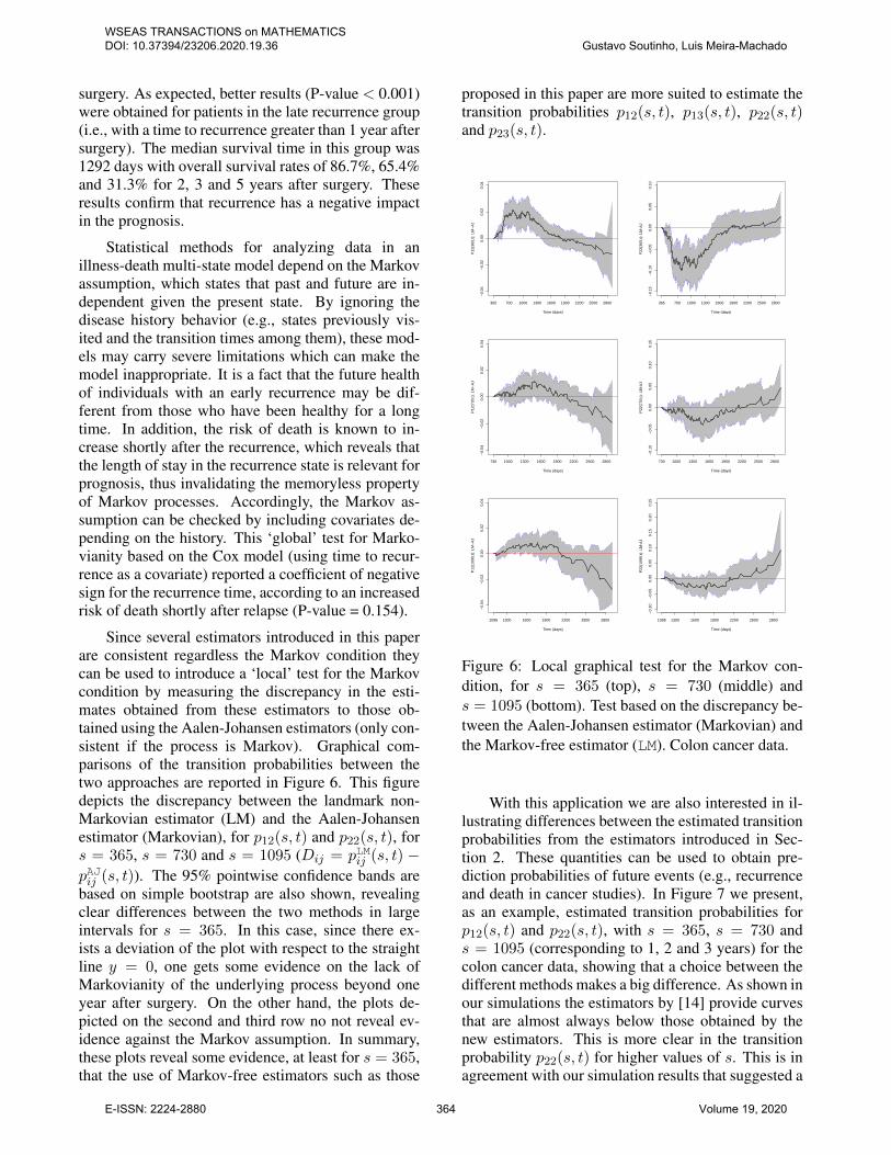
Since several estimators introduced in this paperare consistent regardless the Markov condition theycan be used to introduce a ‘local’ test for the Markovcondition by measuring the discrepancy in the esti-mates obtained from these estimators to those ob-tained using the Aalen-Johansen estimators (only con-sistent if the process is Markov). Graphical com-parisons of the transition probabilities between thetwo approaches are reported in Figure 6. This figuredepicts the discrepancy between the landmark non-Markovian estimator (LM) and the Aalen-Johansenestimator (Markovian), for p12(s, t) and p22(s, t), fors = 365, s = 730 and s = 1095 (Dij = pLMij (s, t) −pAJij (s, t)). The 95% pointwise confidence bands arebased on simple bootstrap are also shown, revealingclear differences between the two methods in largeintervals for s = 365. In this case, since there ex-ists a deviation of the plot with respect to the straightline y = 0, one gets some evidence on the lack ofMarkovianity of the underlying process beyond oneyear after surgery. On the other hand, the plots de-picted on the second and third row no not reveal ev-idence against the Markov assumption. In summary,these plots reveal some evidence, at least for s = 365,that the use of Markov-free estimators such as those

proposed in this paper are more suited to estimate thetransition probabilities p12(s, t), p13(s, t), p22(s, t)and p23(s, t).

−0.

04−

0.02

0.00

0.02

0.04

Time (days)

P12

(365

,t): L

M−

AJ

365 700 1000 1300 1600 1900 2200 2500 2800

−0.

15−

0.10

−0.

050.

000.

050.

10

Time (days)

P22

(365

,t): LM-A

J

365 700 1000 1300 1600 1900 2200 2500 2800

−0.

04−

0.02

0.00

0.02

0.04

Time (days)P

12(7

30,t)

: LM

−A

J

730 1000 1300 1600 1900 2200 2500 2800

−0.

10−

0.05

0.00

0.05

0.10

0.15

Time (days)

P22

(730

,t): LM-A

J

730 1000 1300 1600 1900 2200 2500 2800

−0.

04−

0.02

0.00

0.02

0.04

Time (days)

P12

(109

5,t)

: LM

−A

J

1095 1300 1600 1900 2200 2500 2800

−0.

10−

0.05

0.00

0.05

0.10

0.15

0.20

0.25

Time (days)

P22

(109

5,t)

: LM-A

J

1095 1300 1600 1900 2200 2500 2800

Figure 6: Local graphical test for the Markov con-dition, for s = 365 (top), s = 730 (middle) ands = 1095 (bottom). Test based on the discrepancy be-tween the Aalen-Johansen estimator (Markovian) andthe Markov-free estimator (LM). Colon cancer data.

With this application we are also interested in il-lustrating differences between the estimated transitionprobabilities from the estimators introduced in Sec-tion 2. These quantities can be used to obtain pre-diction probabilities of future events (e.g., recurrenceand death in cancer studies). In Figure 7 we present,as an example, estimated transition probabilities forp12(s, t) and p22(s, t), with s = 365, s = 730 ands = 1095 (corresponding to 1, 2 and 3 years) for thecolon cancer data, showing that a choice between thedifferent methods makes a big difference. As shown inour simulations the estimators by [14] provide curvesthat are almost always below those obtained by thenew estimators. This is more clear in the transitionprobability p22(s, t) for higher values of s. This is inagreement with our simulation results that suggested a


E-ISSN: 2224-2880 364 Volume 19, 2020

systematic negative bias for the estimator by [14] (i.e.a downward biased estimator).

500 1000 1500 2500 3000

0.00

0.05

0.10

0.15

2000

p12(

365,

t)

AJLIDAcLIDAWCH

500 1000 1500 2500 3000

0.0

0.2

0.4

0.6

0.8

1.0

2000

p22(

365,

t)

AJLIDAcLIDALMWCH

1000 1500 2000 2500 3000

0.00

0.02

0.04

0.06

0.08

p12(

730,

t)

AJLIDAcLIDAWCH

1000 1500 2000 2500 3000

0.0

0.2

0.4

0.6

0.8

1.0

p22(

730,

t)

AJLIDAcLIDALMWCH

1500 2000 2500 3000

0.00

0.02

0.04

0.06

0.08

p12(

1095

,t)

AJLIDAcLIDAWCH

1500 2000 2500 3000

0.0

0.2

0.4

0.6

0.8

1.0

p22(

1095

,t)

AJLIDAcLIDALMWCH

Figure 7: Estimated transition probabilities forp12(s, t) and p22(s, t), s = 365 (top), s = 730 (mid-dle) and s = 1095 (bottom). Colon cancer data.

Since few events (‘death’) are observed at highertime values, consistency problems are expected at theright tail of the distribution when using the estima-tor by [14]. These features can be seen in all plotsbut especially in the figures of the transition probabil-ity p22(s, t). While both LM and WCH estimators de-crease smoothly with time the estimator by [14] showsa sharp decrease to zero.

All plots depicted in right hand side of Figure 7reveal a similar behavior of the LM and WCH estima-tors of the transition probability p22(s, t). These plotsreport the survival fraction along time, among the in-dividuals in the recurrence state 1 year (Figure 7, top),and 2 years (Figure 7, middle) and 3 years (Figure 7,bottom) after surgery. They reveal that patients withan early recurrence have lower survival probabilities.When comparing the two Markov-free methods withthe Aalen-Johansen estimator (AJ) one can observesome differences for s = 365 which are less evident ass increases. These discrepancies can be explained by

the failure of the Markov assumption as shown in Fig-ure 6. Similarly, differences can also be observed be-tween AJ and WCH estimators for the transition prob-ability p12(s, t). Summarizing, it becomes clear fromthis application that, at least for s = 365, the use ofMarkov-free estimators such as LM and WCH are pre-ferred over the Aalen-Johansen estimator.

5 Discussion

There has been a remarkable surge of activity latelyon the topic of nonparametric estimation of transi-tion probabilities in multi-state models. Most recentcontributions on this topic are in the context of non-Markov multi-state models since the Aalen-Johansenestimator is still the preferred and standard estimatorwhen one is confident of the Markov assumption. Onerecent paper has used the idea of subsampling to in-troduce estimators that are consistent regardless theMarkov condition. In this paper we propose new es-timators which are constructed using the cumulativehazard of the total time given a first time but whereeach observation has been weighted using the infor-mation of the first duration. Results obtained fromseveral simulation studies conducted under differentdata scenarios show that the new method and the pro-posals introduced by [16] are quite similar providingaccurate estimates.

The comparison between estimated transitionprobabilities is the basis to introduce a graphical lo-cal test for the Markov assumption. The new meth-ods are based on measuring the discrepancy of theAalen-Johansen estimator which gives consistent es-timators in Markov processes, and recent approachesthat do not rely on this assumption. Our simulation re-sults indicated that the Aalen-Johansen estimator pro-vides biased estimates if the Markov assumption doesnot hold. In most of these cases the use of a non-Markov estimator is preferable due to their greater ac-curacy. Therefore, one important issue is how to testthe Markov assumption. Results reported in our dataillustration reveal that the use of a local graphical testcan lead to more reliable conclusions than those ob-tained by a global test such as the one studying Marko-vianity through covariates depending on history.

Acknowledgements: This research was financed byPortuguese Funds through FCT “Fundacao para aCiencia e a Tecnologia”, within the research grantPD/BD/142887/2018.


E-ISSN: 2224-2880 365 Volume 19, 2020

References:

[1] P. K. Andersen and Ø. Borgan and R. D. Gill and N.Keiding, Statistical Models Based on Counting Pro-cesses, Statistics in Medicine, Springer-Verlag, NewYork, 1993.

[2] Hougaard, P., Multi-state Models: a Review, LifetimeData Analysis, 5, pp. 239–264, 1999.

[3] Meira-Machado, L. and de Una-Alvarez, J. andCadarso-Suarez, C. and Andersen, P.K., Multi-statemodels for the analysis of time to event data, Statis-tical Methods in Medical Research, 18, pp. 195–222,2009.

[4] Meira-Machado, L. and Sestelo, M., Estimation in theprogressive illness-death model: A nonexhaustive re-view, Biometrical Journal, 18, pp. 195–222, 2018.

[5] Gentleman, R.C. and Lawless, F.F. and Lindsey, J.C.and Yan, P., Multi-state Markov models for analysingincomplete disease history data with illustrations forHIV disease, Statistics in Medicine, 13, pp. 805-821,1994.

[6] Andersen, P.K. and Esbjerj, S. and Sorensen, T.I.A.,Multistate models for bleeding episodes and mortalityin liver cirrhosi, Statistics in Medicine, 19, pp. 587–599, 2000.

[7] Perez-Ocon, R. and Ruiz-Castro, J.E. and Gamiz-Perez, M.L., Non-homogeneous Markov models inthe analysis of survival after breast cancer, Journal ofthe Royal Statistical Society: Series C, 50, pp. 111–124, 2001.

[8] Putter, H. and Fiocco, M. and Geskus, R. B., Non-homogeneous Markov models in the analysis of sur-vival after breast cancer, Tutorial in biostatistics:Competing risks and multi-state models, 26, 2007.

[9] Aalen, O. and Johansen, S., An Empirical transi-tion matrix for non homogeneous Markov and chainsbased on censored observations, Scandinavian Jour-nal of Statistics, 5, 141–150, 1978.

[10] Moreira, A. and de Una-Alvarez, J. and Meira-Machado, L., Presmoothing the Aalen-Johansen esti-mator in the illness-death model, Electronical Journalof Statistics, 7, 1491–1516, 2013.

[11] Datta, S. and Satten, G.A., Validity of the Aalen-Johansen estimators of stage occupation probabili-ties and Nelson Aalen integrated transition hazardsfor non-Markov models, Statistics & Probability Let-ters, 55, 403–411, 2001.

[12] Datta, S. and Satten, G. A., Estimation of integratedtransition hazards and stage occupation probabilitiesfor non-Markov systems under dependent censoring,Biometrics, 58, 792–802, 2002.

[13] Glidden, D., Robust inference for event probabilitieswith non-Markov event data, Biometrics, 58, 361–368, 2002.

[14] Meira-Machado, L. and de Una-Alvarez, J. andCadarso-Suarez, C., Nonparametric Estimation ofTransition Probabilities in a Non-Markov Illness-Death Model, Lifetime Data Analysis, 12, 325–344,2006.

[15] Allignol, A. and Beyersmann, J. and Gerds, T. andLatouche, A., Nonparametric Estimation of Tran-sition Probabilities in a Non-Markov Illness-DeathModel, Lifetime data analysis, 20, 495–513, 2014.

[16] de Una-Alvarez, J. and Meira-Machado, L., Non-parametric estimation of transition probabilities inthe non-Markov illness-death model: A comparativestudy, Biometrics, 2, 364–375, 2015.

[17] Putter, H. and Spitoni, C., Non-parametric estima-tion of transition probabilities in non-Markov multi-state models: The landmark Aalen-Johansen esti-mator, Statistical Methods in Medical Research, 27,2081–2092, 2018.

[18] Borgan Ø., Aalen-Johansen Estimator, Encyclopediaof Biostatistics, 1, 5–10, 1988.

[19] Kaplan, E.L. and Meier, P., Nonparametric estima-tion from incomplete observations, Journal of theAmerican Statistical Association, 53, 457–481, 1958.

[20] Meira-Machado, L., Smoothed landmark estima-tors of the transition probabilities. SORT-Statisticsand Operations Research Transactions, 40, 375–398,2016.

[21] Soutinho, G., Meira-Machado, L. Oliveira, P.,

A

comparison of presmoothing methods in the estima-tion of transition probabilities, Communications inStatistics - Simulation and Computation, 2020. DOI:10.1080/03610918.2020.1762895

[22] Cox, D.R., Regression models and life tables, Journalof the Royal Statistical Society Series B, 34, 187–220,1972.

[23] Moertel , C. G. and Fleming , Thomas R. and Mac-donald , J. S. and Haller , D. G. and Laurie, J. A. andGoodman , P. J. and Ungerleider , J. S. and Emer

-

son , W. A. and Tormey , D. C. and Glick , J. H. andVeeder , M. H. and Mailliard , J. A., Levamisole andFluorouracil for Adjuvant Therapy of Resected ColonCarcinoma, New England Journal of Medicine, 322,352-358, 1990


E-ISSN: 2224-2880 366 Volume 19, 2020

Documents

Estimation of the Transition Probabilities in Multi-state