Remote Sensing of Environment 119 (2012) 148–157

Contents lists available at SciVerse ScienceDirect

Remote Sensing of Environment

j ourna l homepage: www.e lsev ie r .com/ locate / rse

Estimation of forest resources from a country wide laser scanning survey and nationalforest inventory data

Thomas Nord-Larsen ⁎, Johannes SchumacherUniversity of Copenhagen, Forest and Landscape, 23 Rolighedsvej, DK-1958 Frederiksberg C, Denmark

⁎ Corresponding author. Tel.: +45 35331758.E-mail address: tnl@life.ku.dk (T. Nord-Larsen).

0034-4257/$ – see front matter © 2012 Elsevier Inc. Alldoi:10.1016/j.rse.2011.12.022

a b s t r a c t

a r t i c l e i n f o

Article history:Received 2 September 2011Received in revised form 20 December 2011Accepted 23 December 2011Available online 26 January 2012

Keywords:LiDARModelBasal areaVolumeBiomass

The demand for renewable energy has raised a need for efficient mapping of forest fuel resources in Denmark.Airborne laser scanning may provide a means for assessing local forest biomass resources. In this study, na-tional forest inventory (NFI) data was used as reference data for modeling forest basal area, volume, above-ground biomass, and total biomass from laser scanning data obtained in a countrywide scanning survey. Datacovered a wide range of forest ecotypes, stand treatments, tree species, and tree species mixtures. The fourforest characteristics were modeled using nonlinear regression and generalized method-of-moments estima-tion to avoid biased and inefficient estimates. The coefficient of determination was 68% for the basal areamodel and 77–78% for the volume and biomass models. Despite the wide range of forest types model accu-racy was comparable to similar studies. Model predictions were unbiased across the range of predicted valuesand crown cover percentages but positively biased for deciduous forest and negatively biased for coniferousforest. Species type specific (coniferous, deciduous, or mixed forest) models reduced root mean squared errorby 3–12% and removed the bias. In application, model predictions will be improved by stratification into de-ciduous and coniferous forest using e.g. infrared orthophotos or satellite images.

© 2012 Elsevier Inc. All rights reserved.

1. Introduction

The commitment to the Kyoto Protocol has spurred a widespreadconversion to renewable sources of energy as a means of reducing an-thropogenic emissions of carbon dioxide. In Denmark, this has resultedin an increase in primary energy production in Denmark from forest bio-mass from 18 PJ in 1990 to 41 PJ in 2008 (Danish Energy Agency, 2009).The increase in the use of forest biomass for energy has created a concernthat the resources may not be sufficient to meet the demand and a needfor efficient location–allocation of conversion facilities and forest fuel re-sources. The dispersed nature of the forest fuel resource in Denmark hasraised an interest in mapping of local forest resources in relation to thebiomass supply problem. The Danish National Forest Inventory (NFI,Nord-Larsen et al., 2008) may be used for estimating regional availabilityof forest biomass, but the sampling design does not allow accurate esti-mation of the local potential for procurement of forest biomass forenergy.

Several studies have focused on the assessment of forest resourcesusing airborne laser scanning (ALS). ALS used in forest inventory cap-tures the three-dimensional forest canopy structure and makes use ofthe relationship between canopy structure and other forest proper-ties. A number of studies have shown that mapping of forest volumeand biomass using ALS may yield a satisfactory level of precision and

rights reserved.

accuracy at the forest stand level (e.g. Holmgren & Jonsson, 2004;Lefsky et al., 1999; Lim & Treitz, 2004; Lim et al., 2003; Næsset,1997, 2004b; Patenaude et al., 2004). In a number of Nordic studiesthe reported RMSE of basal area and volume was 8.6–13.2% and8.4–42.7% of the mean, respectively (Næsset, 2007; Næsset et al.,2004).

The notion that sufficient accuracy may be obtained from estimat-ing local forest resources using ALS has motivated applications inlarge scale forest inventory. In a first attempt to apply ALS in forest in-ventory, Næsset, (2002) used a two-stage procedure in a 10 km2

study area and obtained a high level of precision. Since then ALS hasbeen used operationally to estimate forest resources in areas rangingfrom 50 to 2000 km2 (Næsset, 2007; Næsset et al., 2009). These stud-ies have proven ALS to be a cost effective method for obtaining bio-physical forest properties such as forest volume or biomass (Eidet al., 2004). However, complete scanning of larger regions may notbe economically feasible using the hitherto used procedures due tothe costs of acquisition and processing the large amounts of data as-sociated with this technique.

In recent studies, laser technology has been expanded to entire re-gions, using airborne laser scanning and/or laser profiling as samplingtools. Boudreau et al. (2008, 2009) combined several sources of infor-mation including small footprint airborne profiling laser data andlarge footprint spaceborne laser to estimate above ground dry bio-mass in Québec covering 1.3 M km2. In this study, data from the pro-filing laser was used as auxiliary data for developing equationsrelating spaceborne laser pulse data to biomass and carbon pools.

Table 1Summary of the laser scanner and flight data.

System Optech ALTM 3100Flying altitude 1600 mPulse repetition frequency 70 kHzScanning angle ±24∘

Average point density 0.5 pulse/m2

Footprint size 50 cmHorizontal accuracy 80 cm (1σ)Vertical accuracy 10 cm (1σ)

149T. Nord-Larsen, J. Schumacher / Remote Sensing of Environment 119 (2012) 148–157

Gregoire et al. (2011) and Ståhl et al. (2011) compared the use ofboth a profiling laser and ALS as a strip sampling tool for inventoryingtimber volume and biomass in large areas.

Rather than reducing the area covered by the laser scanner (i.e. byusing profiling laser or strip sampling with a laser scanner), the costsof data acquisition and handling may be reduced by increasing flyingaltitude (Næsset, 2004a; Yu et al., 2004) and/or the scanning angle(Holmgren et al., 2003) hereby increasing the average point spacing(Thomas et al., 2006). Also, costs may be reduced by using dataobtained in relation to other surveys, such as mapping terrain orother geographical features. In this study we hypothesize that ALSdata obtained in a large regional survey for obtaining a digital terrainmodel (DTM) in combination with national forest inventory (NFI)data may be used for developing remote sensing tools for estimationof forest basal area, volume, above ground biomass, and total bio-mass. The overreaching objective of the study concerns the use ofwall-to-wall ALS data for assessing biofuel resources in Denmark.More specifically, the objectives of the study are to combine wall-to-wall ALS data with NFI data for 1) developing regression modelsto predict forest basal area, volume and biomass, 2) assessing thegoodness of the parameterized models, and 3) evaluating model per-formance on an independent data.

2. Materials and methods

2.1. Laser scanning data

The entire Danish land surface was scanned in 2006–2007 withthe aim to improve existing DTM's (COWI, 2007a). The scanningwas conducted in two surveys during leaf-off conditions in spring2006 and fall 2006/spring 2007. First and last return pulses wererecorded by the scanner. A summary of the laser scanner and flightdata is provided in Table 1.

The resulting point cloud was tested for geometrical accuracyusing ground based data and a DTM was generated from the pointcloud using TerraScan software. The generation of the DTM and test-ing of the point cloud data was carried out by COWI A/S (COWI,2007b). Based on the DTM, the elevation above ground (Dz) was cal-culated for each point in the point cloud.

The first and last return pulses were spatially assigned to the sam-ple plots of the national forest inventory. For each individual plot, a

Table 2Laser scanning data statistics for first and last return pulses from all plots used in model es

Variable First return

Mean Std. dev.

Returns 452.1 161.1Returns (>1 m) 248.6 165.4Average return pulse height 6.6 5.7Average return pulse height (>1 m) 9.9 5.8Max return pulse height 15.6 8.0Canopy interception ratio 56.3 31.2Average return pulse intensity 18.7 7.9Average return pulse intensity (>1 m) 11.8 7.2Max return pulse intensity 42.0 12.7

large number of metrics were derived from the pulse height aboveground distributions as potential variables for modeling aboveground volume and biomass. The metrics were calculated on boththe first (r=1) and last return pulse data (r=2), and both with(Dz≥0 m; q=1) and without ground hits (Dz>1 m; q=2).

The metrics include: 1) Mean, maximum and minimum pulseheight above ground (Dzmean, r, q, Dzmax, r, q, and Dzmin, r, q), 2) variance,standard deviation, and coefficient of variation (Dzvar, r, q, Dzstd, r, q,and Dzcv, r, q), 3) skewness and kurtosis (Dzskew, r, q and Dzkur, r, q), 4)distribution percentiles (Dzp, r, q; p=10, 25, 50, 75, 90, 95, 99), 5) rel-ative mean and median height (the mean and median pulse heightabove ground relative to maximum pulse height; Dzrelmean, r,q and Dz-relmed, r,q), and 6) canopy interception ratio (the number of pulsesreflected from above ground (Dz>1 m) relative to the total numberof pulses; IRr).

Additionally, the vertical space betweenDzmax and the groundwas di-vided into 10 strata where {Dzh|Dzmax/10⋅h≥Dzh>Dzmax/10⋅(h−1)},h=1,2,⋯10. For each stratum we calculated 7) the interception ratio(the number of pulses reflected from stratum h relative to the total num-ber of pulses; IR(h), r) and 8) variance and distribution form parameters(Dzcv(h), r,q, Dzskew(h), r,q, and Dzkurt(h), r,q). Further, similar statistics werederived for the intensity of the reflections from the canopy, labeled IN.In this study we used the uncalibrated return pulse intensities asrecorded by the scanning equipment. Such intensities have beenreported to be noisy and varying with the range to the reflecting object(Höfle & Pfeifer, 2007; Kaasalainen et al., 2005). It is possible to correctthe raw pulse intensities using range normalization (Korpela et al.,2010) but we lacked sufficient information to make such adjustments.However, the Danish terrain is quite flat and consequently the range var-iation and thus the possible corrections are likely to be relatively small(b10%).

The resulting ALS meta data includes metrics from a total of 2265national forest inventory plots selected for inventory during the peri-od 2006–2007, corresponding to the time of the laser scanning sur-vey. In a study using the same data for modeling canopy heightfrom laser scanning data (Nord-Larsen & Riis-Nielsen, 2010), outlierswere identified that resulted from crowns of neighboring trees reach-ing into and dominating the sample plots and logging that had hap-pened between the time of the laser scanning and the time ofground data collection. A total of 87 outliers were identified and re-moved from the calibration data. Further, in 48 plots more than 10%of return pulses were erroneously recorded from below ground andthese plots were removed from the calibration data. The resultingdataset contains data from 2130 plots inventoried in the field andtheir corresponding laser scanning data (Table 2).

2.2. Forest inventory data

The Danish NFI is based on a 2×2 km grid placed over the Danishland surface. In each grid cell, a cluster of four circular plots for mea-suring forest factors (e.g. growing stock, biomass, or carbon stock) is

timation (N=2130). ‘Returns’ are the number of returns per plot.

Last return

Range Mean Std. dev. Range

27–1536 460.6 145.3 96–14090–1281 125.0 140.3 0–829

0.0–30.1 2.8 3.9 0.0–27.51.0–31.7 8.3 5.5 1.0–29.20.0–42.1 13.3 8.3 0.0–40.20.0–100.0 27.0 27.1 0.0–97.72.8–48.4 206.9 72.2 28.5–511.61.4–40.2 156.6 66.7 10.0–402.1

14.0–260.0 421.9 130.6 140.0–2600.0

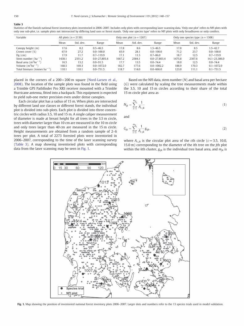
Table 3Statistics of the Danish national forest inventory plots inventoried in 2006–2007. Includes only plots with corresponding laser scanning data. ‘Only one plot’ refers to NFI plots withonly one sub-plot, i.e. sample plots not intersected by differing land uses or forest stands. ‘Only one species type’ refers to NFI plots with only broadleaves or only conifers.

Variable All plots (n=2130) Only one plot (n=1267) Only one species type (n=1308)

Mean Std. dev. Range Mean Std. dev. Range Mean Std. dev. Range

Canopy height (m) 17.6 8.2 0.5–46.5 17.8 8.6 1.5–46.5 17.8 8.5 1.5–42.7Crown cover (%) 67.9 27.2 0.0–100.0 65.9 28.1 0.0–100.0 71.2 23.7 0.0–100.0Dg (cm) 17.9 11.7 0.7–119.9 17.1 11.5 0.7–86.0 18.7 12.5 0.7–119.9Stem number (ha−1) 1438.1 2351.2 0.0–27,803.4 1667.2 2584.1 0.0–27,803.4 1475.8 2307.6 14.1–23,386.0Basal area (m2ha−1) 16.5 13.2 0.0–91.5 17.7 13.5 0.0–74.4 18.0 12.5 0.0–74.4Volume (m3ha−1) 168.5 169.3 0.0–1072.0 182.7 177.6 0.0–1002.2 188.9 170.3 0.1–1072.0Total biomass (tonnes ha−1) 110.1 110.1 0.0–751.5 118.7 114.0 0.0–666.0 123.0 111.1 0.1–751.5

150 T. Nord-Larsen, J. Schumacher / Remote Sensing of Environment 119 (2012) 148–157

placed in the corners of a 200×200 m square (Nord-Larsen et al.,2008). The location of the sample plots was found in the field usinga Trimble GPS Pathfinder Pro XRS receiver mounted with a TrimbleHurricane antenna, fitted into a backpack. This equipment is expectedto yield sub-one meter precision even under dense canopies.

Each circular plot has a radius of 15 m. When plots are intersectedby different land use classes or different forest stands, the individualplot is divided into sub-plots. Each plot is divided into three concen-tric circles with radius 3.5, 10 and 15 m. A single caliper measurementof diameter is made at breast height for all trees in the 3.5 m circle,trees with diameter larger than 10 cm are measured in the 10 m circleand only trees larger than 40 cm are measured in the 15 m circle.Height measurements are obtained from a random sample of 2–6trees per plot. A total of 2273 forested plots were inventoried in2006–2007, corresponding to the time of the laser scanning survey(Table 3). A map showing inventoried plots with correspondingdata from the laser scanning may be seen in Fig. 1.

Fig. 1. Map showing the position of inventoried national forest inventory plots 2006–20

Based on the NFI data, stem number (N) and basal area per hectare(G) were calculated by scaling the tree measurements made withinthe 3.5, 10 and 15 m circles according to their share of the total15 m circle plot area as

Njk ¼Xmjk

i¼1

1Ac; jk

ð1Þ

and

Gjk ¼Xmjk

i¼1

1Ac; jk

gijk; ð2Þ

where Ac, jk is the circular plot area of the cth circle (c=3.5, 10.0,15.0 m) corresponding to the diameter of the ith tree on the jth plotwithin the kth cluster, gijk is the individual tree basal area, and mjk is

07. Larger dots and numbers refer to the 13 species trials used in model validation.

151T. Nord-Larsen, J. Schumacher / Remote Sensing of Environment 119 (2012) 148–157

the total number of sampled trees within the plot. Quadratic mean di-ameter was subsequently estimated as

Dg; jk ¼4πGjk

Njk: ð3Þ

Based on the sample tree height measurements, generalized, spe-cies wise dh-regressions were estimated using the approach sug-gested by Sloboda et al. (1993):

hijk ¼ 13þ �hjk−13� �

⋅exp a1 1þ�djk

dijk

!þ a2

1�djk

− 1dijk

! !; ð4Þ

where dijk and hijk are diameter (in mm) and height (in cm) of the ithtree within the jth plot and kth cluster, �djk and �hjk are mean diameterand height, and a1 and a2 are parameters to be estimated. The heightof trees not measured is subsequently estimated using Eq. (4), wherespecies-specific parameters were estimated using data from all treesmeasured for height in the NFI during 2002–2010 (23,645 trees).

Individual tree above ground volume of broadleaves and stem vol-umes of conifers (vijk) were estimated from d, (estimated) h, and Dg,using volume equations developed by Madsen, (1987) and Madsenand Heusérr, (1993). Tree biomass was subsequently estimatedusing species specific wood densities reported by Moltesen, (1988).Above-ground (bag, ijk) and total tree (btotal, ijk) biomass for individualbroadleaf trees was estimated using expansion factors derived forbeech (Skovsgaard & Nord-Larsen, 2011) whereas biomass for conif-erous trees were estimated using expansion factors developed forNorway spruce (Skovsgaard et al., 2011). For both broadleaves andconifers, above ground biomass includes the branches (without fo-liage), stem and above-ground stump. Entire tree biomass further in-cludes the below-ground stump and root system down to anapproximate diameter of 2 mm. Above ground volume (Vjk), above-ground biomass (Bag, jk) and total biomass (Btotal, jk) were finally esti-mated by scaling the tree measurements made within the 3.5, 10.0,and 15.0 m circles according to their share of the total 15 m circleplot area as

Vjk ¼Xmjk

i¼1

1Ac; jk

vijk; ð5Þ

Bag;jk ¼Xmjk

i¼1

1Ac;jk

bag;ijk; ð6Þ

and

Btotal; jk ¼Xmjk

i¼1

1Ac; jk

btotal;ijk; ð7Þ

where symbols are as defined above.

2.3. Permanent sample plot data

Data from permanent sample plots was used for validation of thedeveloped models. Measurements in a forest tree species trial estab-lished in 1965 were carried out in the fall of 2007, almost correspond-ing to the time of acquisition of the laser scanning data. The speciestrial consists of 13 different experimental sites covering the majorgrowth regions in Denmark (Fig. 1) and 156 individual plots. Netplot sizes are about 0.15 ha. The tree species trial includes 12 differentspecies at each site (totaling 15 different tree species) which includethe 13 most commonly grown conifers (Norway spruce (Picea abies(L.) Karst.), Sitka spruce (Picea sitchensis (Bong.) Carr.), Serbianspruce (Picea omorika (Panv cić) Purk.), silver fir (Abies alba Mill.),grand fir (Abies grandis (Douglas ex D. Don) Lindley), noble fir

(Abies procera Rehder), Douglas fir (Pseudotsuga menziesii (Mirb.)Franco), western red cedar (Thuja plicata Donn ex D. Don), Scotspine (Pinus sylvestris L.), French mountain pine (Pinus mugo Turra),lodgepole pine (Pinus contorta Douglas), cypress (Chamaecyparis law-soniana (A. Murray) Parl.), and Japanese larch (Larix kaempferi(Lamb.) Carr.) and the two most commonly grown deciduous species(beech (Fagus sylvatica L.) and oak (Quercus robur L.)).

In the fall of 2007, the species trial included 91 different plots andall the above mentioned species. Remaining plots were lost duringstand establishment or due to catastrophic wind throws. In eachplot all trees were uniquely identified and cross-calipered at breastheight. Height was obtained for a subsample of 30 randomlyselected trees from each plot. Calculations of stand variables weresimilar to those of the NFI data. To obtain an estimate of standvariables at the time of the laser scanning (spring 2007 for allplots), a linear interpolation was made between the state afterthinning in the previous measurement (fall 2001) and the statebefore thinning in the fall 2007.

2.4. Model development

In the first step of selecting predictor variables derived from thelaser scanning data, a correlation matrix (Spearman's rank) of re-sponse variables (stand basal area, volume, or biomass) and potentialpredictor variables was calculated using data from NFI plots with onlyone sub-plot to exclude plots dominated by other land uses. Subse-quently, a cluster analysis was conducted on the correlation matrixto identify groups of variables showing similar correlation structurewith the response variable and among the predictor variables. Thecluster analysis was based on least-squares minimization of the Eu-clidean distances to the cluster centers (k-means model) where thenumber of potential clusters were set at 5 (PROC FASTCLUS, SASInstitute, 2009).

Based on the cluster analysis, the potential predictor variable showingthe highest correlation with the specific response variable within eachcluster was selected, while excluding variables having a similar correla-tion structure. This was done to avoid over-parametrization of themodel. The overall procedure for selecting potential predictor variableswas similar to the method in Nord-Larsen and Riis-Nielsen, (2010).

In the next step of model development we assessed the perfor-mance of a large number of basic model forms in predicting standbasal area, volume, and biomass based on the previously selectedlaser metrics. The tested model forms included several forms of expo-nential and power functions previously used in similar studies. Usingthe procedure described above we found that the multiplicativemodel (Y=α0X1

α1X2α2…Xm

αm, where m is the number of model param-eters) was well suited to predict basal area, volume, above-groundbiomass, and total biomass. Model parameters were estimated usingnonlinear regression of the MODEL procedure in SAS Institute,(2009). As the variance of untransformed data was heteroscedastic,estimates are expected to be unbiased but inefficient. To improve ef-ficiency of the parameter estimation we applied generalized method-of-moments estimation (GMM, Hansen, 1982) as the variance rela-tionship was unknown.

In the final model estimation we initially included all potentialpredictor variables selected from the cluster analysis, and selectedthe final predictor variables using backward elimination of non-significant parameters (P>0.05). Model development was based ondata from plots not divided into subplots (One plot only). This wasdone to capture generic properties of the relationship between vari-ables derived from the laser scanning point cloud and forest biophys-ical properties. Such relationships are likely to be clouded when plotscovering several forest types or even different land uses are included.The parameters of the final model formulations were estimated usingdata from both plots not divided into subplots and from all availableplots to allow for assessment of the effect of including plots covering

152 T. Nord-Larsen, J. Schumacher / Remote Sensing of Environment 119 (2012) 148–157

more than one forest type or different types of land use. Further, apreliminary study revealed that the relationship between laser scan-ning variables and forest properties differed between coniferous anddeciduous forest. Consequently, we estimated models using all dataas well as for individual strata including only coniferous, deciduousor mixed forests. The latter allows for improving model estimateswhen tree species composition is known from forest maps or otherremote sensing efforts.

2.5. Model evaluation

Model errors were first characterized in terms of magnitude anddistribution by plotting residuals against predicted values of basalarea, volume, above-ground biomass, and total biomass per hectare.Furthermore, residuals were plotted against observed values ofother stand variables to expose any obvious trends. Spatial trendswere evaluated by plots of residuals against natural-geographical re-gions of Denmark according to Jacobsen, (1976).

In addition to the visual appraisal of the errors a number of sum-mary statistics were calculated for the entire data set as well as fordifferent strata of the model subject. The summary statistics includeaverage error (AB), average absolute error (AAB), root mean squarederror (RMSE), and coefficient of determination (R2).

Statistical tests ofmodel assumptions on patterns and distribution ofthe residuals as well as model bias and stability, were carried out. Vari-ance homogeneity was tested using a White-test and normality wastested using Andersson–Darling goodness-of-fit test. Model bias wastested using a simultaneous F-tests for unit slope and zero intercept ofthe linear regression of observed versus predicted data (Dent &Blackie, 1979). Predictive performance and stability of the parameterestimateswere evaluated by leave-one-out cross validation inwhich in-dividual NFI plots were left out of the estimation data one at a time andsubsequently the estimated model was applied to the left-out plot.

The models were further evaluated using permanent plot datafrom the species trial established in 1965. When constructing valida-tion data, a square moving window with a size identical to the NFIsample plots (706 m2) was repeatedly sampled among the laser scan-ning data 100 times within each plot and stand variables were esti-mated using the developed models. The average stand variables ofthe 100 estimates were compared with the measured values usingsimilar methods as described above. The method implies that the100 estimates are highly correlated as they are sampled within thesame plot and the samples are partially overlapping. Hence the meth-od yield unbiased mean values but biased estimates of variance.

3. Results

Many of the potential predictor variables were highly correlatedwith the four response variables. For all response variables, the firstreturn mean pulse height above ground (Dzmean, 1, 1 ; j) had the highestcoefficient of correlation (Spearman rank-order) ranging from 0.85(basal area) to 0.93 (volume, above-ground biomass, and total bio-mass). Other variables showing high levels of correlation with thepredictor variables included the relative mean first pulse height(Dzrelmean, 1, 1 ; j), the first pulse interception rate (IR1 ; j), and the 50'th,75'th, and 95'th percentiles of first return pulse heights (Dzp, 1, 1).

The models for predicting basal area, volume, and biomass includ-ed only metrics derived from the first return pulse data. The finalmodel for basal area (G) included the mean pulse height of all first re-turn pulses (Dzmean, 1, 1 ; j), the relative mean height of the laser pulsedistribution (Dzrelmean, 1, 1 ; j), the first pulse interception rate (IR1 ; j),and the coefficient of variation of first return pulse intensities(Incv, 1, 1 ; j):

Gj ¼ γ0⋅Dzγ1mean;1;1; j⋅Dz

γ2relmean;1;1; j⋅IR

γ31; j⋅In

γ4cv;1;1; j þ εG; j; ð8Þ

where εG, j is the random error of the jth plot and γ0−γ4 are param-eters to be estimated.

The volume (V), above ground biomass (Bag), and total biomass(Btotal) models all included the mean height of the first return laserpulse distribution and the 95 percentile of above ground first returnpulses (Dz95, 1, 2 ; j). The volume model included also the first pulse in-terception rate, whereas the two biomass models included the coeffi-cient of variation of first return pulse intensities:

Vj ¼ ν0⋅Dzν1mean;1;1;j⋅Dz

ν295;1;2;j⋅IR

ν31;j þ εV ;j; ð9Þ

Bag;j ¼ α0⋅Dzα1mean;1;1;j⋅Dz

α295;1;2;j⋅In

α3cv;1;1;j þ εBag ;j; ð10Þ

and

Btotal;j ¼ β0⋅Dzβ1mean;1;1;j⋅Dz

β295;1;2;j⋅In

β3cv;1;1;j þ εBtotal ;j: ð11Þ

where εV, j, εBag, j, and εBtotal, j are the random errors of the jth plot andν0−ν3, α0−α3, and β0−β3 are parameters to be estimated. Parameterestimates are provided in Table 4.

Using data from NFI plots with only one sub-plot, the coefficient ofdetermination was 68% for the basal area model and 78% for the vol-ume and biomass models, respectively (Table 5). Scatter plots of re-siduals across predicted values, species groups and observed crowncover revealed no obvious trends (Fig. 2). The distribution of residualsdiffered significantly from normality (Pb0.001) and homogeneityacross predicted values (Pb0.001).

Predictions were unbiased across all observations (P≥0.05), butthe basal area, volume, above ground biomass, and total biomasswere overestimated for deciduous species and underestimated for co-nifers (Pb0.05). Residuals of the three models were generally unbi-ased for different growth regions except for the island of Funen,where basal area, volume and biomass were generally overestimated.We have no explanation for this behavior that was unrelated to spe-cies composition but may be related to forest structure as the forestson Funen are generally small and scattered. Fit statistics were gener-ally little affected when using all plots (i.e. including NFI plots withmore than one sub-plot). The leave-one-out cross validation lead toonly a minor increase in RMSE (−0.8, 0.5, 0.6 and 0.6% for the basalarea, volume, above ground biomass, and total biomass models, re-spectively.) The reason for the small decrease in RMSE of the crossvalidation for the basal area model may be due to failure to convergein 6 cases of the 1267 iterations of the procedure.

The observed bias for different species types (broadleaves, coni-fers, and mixed forest) indicate that models could be improved by es-timation of species type specific models. Such models could beemployed when additional information on species is available e.g.from stand inventories or different types of remote sensing. Wethus estimated the models in Eqs. (8), (9), (10), and (11) for the indi-vidual tree species types using the one-plot only data. Using the spe-cies specific estimates reduced overall RMSE of the basal area,volume, above ground biomass, and total biomass models by 12, 7,4, and 3%, respectively and the previously observed bias was unobser-vable (Table 6).

The models were validated using data from the species trials andcorresponding laser scanning data. When applying the generalmodels (Table 4), the coefficient of determination was 0.61, 0.75,0.58, and 0.59 for the basal area, volume, above ground biomass andtotal biomass respectively, and the previously mentioned bias forbroadleaves and conifers was very pronounced (not shown). Whenapplying the species specific models (Table 6), the coefficient of de-termination was 0.77, 0.77, 0.66, and 0.69 for the basal area, volume,above ground biomass and total biomass respectively. Models for vol-ume and biomass were largely unbiased, whereas the model overes-timated basal area (Fig. 3). For some plots with a very large growing

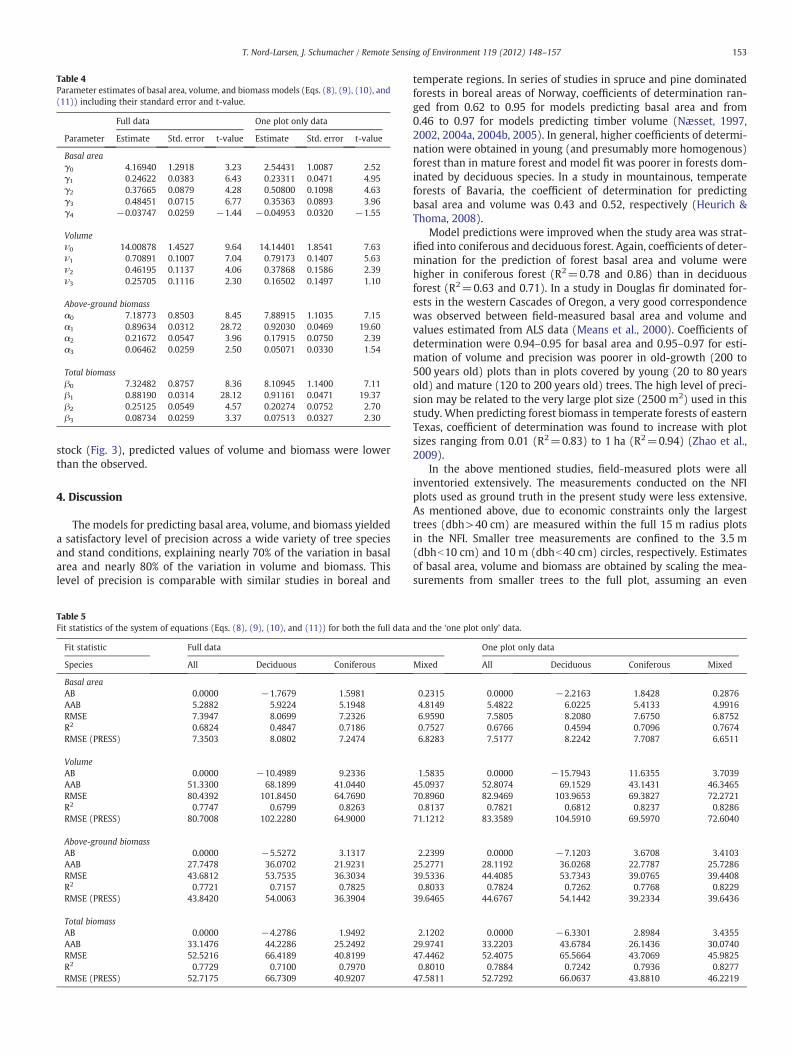
Table 4Parameter estimates of basal area, volume, and biomass models (Eqs. (8), (9), (10), and(11)) including their standard error and t-value.

Full data One plot only data

Parameter Estimate Std. error t-value Estimate Std. error t-value

Basal areaγ0 4.16940 1.2918 3.23 2.54431 1.0087 2.52γ1 0.24622 0.0383 6.43 0.23311 0.0471 4.95γ2 0.37665 0.0879 4.28 0.50800 0.1098 4.63γ3 0.48451 0.0715 6.77 0.35363 0.0893 3.96γ4 −0.03747 0.0259 −1.44 −0.04953 0.0320 −1.55

Volumeν0 14.00878 1.4527 9.64 14.14401 1.8541 7.63ν1 0.70891 0.1007 7.04 0.79173 0.1407 5.63ν2 0.46195 0.1137 4.06 0.37868 0.1586 2.39ν3 0.25705 0.1116 2.30 0.16502 0.1497 1.10

Above-ground biomassα0 7.18773 0.8503 8.45 7.88915 1.1035 7.15α1 0.89634 0.0312 28.72 0.92030 0.0469 19.60α2 0.21672 0.0547 3.96 0.17915 0.0750 2.39α3 0.06462 0.0259 2.50 0.05071 0.0330 1.54

Total biomassβ0 7.32482 0.8757 8.36 8.10945 1.1400 7.11β1 0.88190 0.0314 28.12 0.91161 0.0471 19.37β2 0.25125 0.0549 4.57 0.20274 0.0752 2.70β3 0.08734 0.0259 3.37 0.07513 0.0327 2.30

153T. Nord-Larsen, J. Schumacher / Remote Sensing of Environment 119 (2012) 148–157

stock (Fig. 3), predicted values of volume and biomass were lowerthan the observed.

4. Discussion

The models for predicting basal area, volume, and biomass yieldeda satisfactory level of precision across a wide variety of tree speciesand stand conditions, explaining nearly 70% of the variation in basalarea and nearly 80% of the variation in volume and biomass. Thislevel of precision is comparable with similar studies in boreal and

Table 5Fit statistics of the system of equations (Eqs. (8), (9), (10), and (11)) for both the full data

Fit statistic Full data

Species All Deciduous Coniferous

Basal areaAB 0.0000 −1.7679 1.5981AAB 5.2882 5.9224 5.1948RMSE 7.3947 8.0699 7.2326R2 0.6824 0.4847 0.7186RMSE (PRESS) 7.3503 8.0802 7.2474

VolumeAB 0.0000 −10.4989 9.2336AAB 51.3300 68.1899 41.0440RMSE 80.4392 101.8450 64.7690R2 0.7747 0.6799 0.8263RMSE (PRESS) 80.7008 102.2280 64.9000

Above-ground biomassAB 0.0000 −5.5272 3.1317AAB 27.7478 36.0702 21.9231RMSE 43.6812 53.7535 36.3034R2 0.7721 0.7157 0.7825RMSE (PRESS) 43.8420 54.0063 36.3904

Total biomassAB 0.0000 −4.2786 1.9492AAB 33.1476 44.2286 25.2492RMSE 52.5216 66.4189 40.8199R2 0.7729 0.7100 0.7970RMSE (PRESS) 52.7175 66.7309 40.9207

temperate regions. In series of studies in spruce and pine dominatedforests in boreal areas of Norway, coefficients of determination ran-ged from 0.62 to 0.95 for models predicting basal area and from0.46 to 0.97 for models predicting timber volume (Næsset, 1997,2002, 2004a, 2004b, 2005). In general, higher coefficients of determi-nation were obtained in young (and presumably more homogenous)forest than in mature forest and model fit was poorer in forests dom-inated by deciduous species. In a study in mountainous, temperateforests of Bavaria, the coefficient of determination for predictingbasal area and volume was 0.43 and 0.52, respectively (Heurich &Thoma, 2008).

Model predictions were improved when the study area was strat-ified into coniferous and deciduous forest. Again, coefficients of deter-mination for the prediction of forest basal area and volume werehigher in coniferous forest (R2=0.78 and 0.86) than in deciduousforest (R2=0.63 and 0.71). In a study in Douglas fir dominated for-ests in the western Cascades of Oregon, a very good correspondencewas observed between field-measured basal area and volume andvalues estimated from ALS data (Means et al., 2000). Coefficients ofdetermination were 0.94–0.95 for basal area and 0.95–0.97 for esti-mation of volume and precision was poorer in old-growth (200 to500 years old) plots than in plots covered by young (20 to 80 yearsold) and mature (120 to 200 years old) trees. The high level of preci-sion may be related to the very large plot size (2500 m2) used in thisstudy. When predicting forest biomass in temperate forests of easternTexas, coefficient of determination was found to increase with plotsizes ranging from 0.01 (R2=0.83) to 1 ha (R2=0.94) (Zhao et al.,2009).

In the above mentioned studies, field-measured plots were allinventoried extensively. The measurements conducted on the NFIplots used as ground truth in the present study were less extensive.As mentioned above, due to economic constraints only the largesttrees (dbh>40 cm) are measured within the full 15 m radius plotsin the NFI. Smaller tree measurements are confined to the 3.5 m(dbhb10 cm) and 10 m (dbhb40 cm) circles, respectively. Estimatesof basal area, volume and biomass are obtained by scaling the mea-surements from smaller trees to the full plot, assuming an even

and the ‘one plot only’ data.

One plot only data

Mixed All Deciduous Coniferous Mixed

0.2315 0.0000 −2.2163 1.8428 0.28764.8149 5.4822 6.0225 5.4133 4.99166.9590 7.5805 8.2080 7.6750 6.87520.7527 0.6766 0.4594 0.7096 0.76746.8283 7.5177 8.2242 7.7087 6.6511

1.5835 0.0000 −15.7943 11.6355 3.703945.0937 52.8074 69.1529 43.1431 46.346570.8960 82.9469 103.9653 69.3827 72.27210.8137 0.7821 0.6812 0.8237 0.8286

71.1212 83.3589 104.5910 69.5970 72.6040

2.2399 0.0000 −7.1203 3.6708 3.410325.2771 28.1192 36.0268 22.7787 25.728639.5336 44.4085 53.7343 39.0765 39.44080.8033 0.7824 0.7262 0.7768 0.8229

39.6465 44.6767 54.1442 39.2334 39.6436

2.1202 0.0000 −6.3301 2.8984 3.435529.9741 33.2203 43.6784 26.1436 30.074047.4462 52.4075 65.5664 43.7069 45.98250.8010 0.7884 0.7242 0.7936 0.8277

47.5811 52.7292 66.0637 43.8810 46.2219

Fig. 2. Residuals of the basal area, volume and biomass models. Based on the one plot only data (1345 observations).

154 T. Nord-Larsen, J. Schumacher / Remote Sensing of Environment 119 (2012) 148–157

distribution across the plot. This stratification of measurements in theNFI introduces additional error to the dependent variables affectingthe observed model precision negatively. We therefore expect thatactual model precision may be even higher than estimated.

Compared to similar studies, the variability of the study object wasquite large. The data covered a wide ecological gradient from sandyoutwash planes in western Jutland, to fertile tills in the eastern partof the country. The sample plots used in the analysis included atotal of 56 different forest tree species, about 73% of the plots con-tained mixtures of different species and 39% of the plots had mixturesof broadleaves and conifers. The majority of forest stands included inthis study had fully closed canopies (25% had a crown cover of morethan 90%), but 20% had a crown cover of less than 50%.

Although the model yielded a satisfactory level of precision acrossthe entire data, predictions were positively biased for broadleavesand negatively biased for conifers. This bias is possibly caused by dif-ferences in morphology of the different tree species, which was ac-centuated by the capture of laser scanning data during leaf-offconditions and is similar to the findings of other authors (Næsset,2005; Næsset & Gobakken, 2008). Rigorous analysis did not reveal pa-rameters suited for capturing the inter-species differences such as forindividual trees in Brandtberg, (2007), Brandtberg et al., (2003),Holmgren and Persson, (2004), Holmgren et al., (2008), Korpela etal., (2010), Örka et al., (2009), Reitberger et al., (2008) and indicatea potential for stratifying measurements according to species typeas also done by some authors (Heurich & Thoma, 2008; Næsset &

Table 6Species specific parameter estimates of basal area, volume, and biomass models(Eqs. (8), (9), (10), and (11)) including their standard error. Models were estimatedwith the one-plot-only data. Fit statistics are provided for the full data set and forthe individual species types.

Broadleaves Conifers Mixtures

Parameter Estimate Std. error Estimate Std. error Estimate Std. error

Basal area (AB=0.0000, AAB=4.7931, RMSE=6.6995, R2=0.7474)γ0 1.22817 0.7027 1.64305 1.0451 2.40998 1.5943γ1 0.31337 0.0672 0.46101 0.0704 0.38049 0.0798γ2 0.29510 0.1546 0.67545 0.1486 0.48636 0.1724γ3 0.18779 0.1456 −0.11357 0.1023 0.33665 0.1723γ4 0.22497 0.0437 −0.23295 0.0753 −0.08839 0.0635AB 0.0000 0.0000 0.0000AAB 4.9356 4.7181 4.7265RMSE 6.8185 6.6944 6.6841R2 0.6269 0.7791 0.7801

Volume (AB=0.0000, AAB=48.7216, RMSE=77.4627, R2=0.8099)ν0 10.82550 2.2564 19.68917 3.4980 15.40511 4.0804ν1 0.66846 0.1775 1.92446 0.1442 1.34476 0.2707ν2 0.53376 0.1959 −0.71557 0.1637 −0.12397 0.3013ν3 0.00756 0.2057 −0.89276 0.1120 −0.26717 0.2883AB 0.0000 0.0000 0.0000AAB 65.0859 38.1463 43.2479RMSE 98.6859 60.8475 69.1138R2 0.7127 0.8644 0.8433

Above-ground biomass (AB=0.0000, AAB=27.2572, RMSE=42.7447, R2=0.7984)α0 2.75662 0.7882 17.61783 5.3287 11.07974 3.3571α1 0.80103 0.0658 1.10166 0.0846 1.10137 0.1002α2 0.39316 0.1107 0.00597 0.1337 0.05088 0.1642α3 0.19563 0.0470 −0.12862 0.1088 −0.03363 0.0682AB 0.0000 0.0000 0.0000AAB 34.6985 22.5133 24.6963RMSE 51.5663 37.6862 38.1034R2 0.7478 0.7924 0.8347

Total biomass (AB=0.0000, AAB=32.3332, RMSE=50.7500, R2=0.8016)β0 3.52007 1.0183 20.23273 5.8492 11.80632 3.5527β1 0.78434 0.0657 1.09759 0.0825 1.09657 0.1000β2 0.39255 0.1114 0.03838 0.1295 0.05904 0.1646β3 0.19566 0.0475 −0.14571 0.1027 −0.01087 0.0673AB 0.0000 0.0000 0.0000AAB 42.6714 25.5764 28.9591RMSE 63.7448 41.9969 44.4936R2 0.7393 0.8095 0.8387

155T. Nord-Larsen, J. Schumacher / Remote Sensing of Environment 119 (2012) 148–157

Gobakken, 2008). Estimating equations for the two species types indi-vidually led to a reduction in RMSE of 3–17% for broadleaves and4–13% for conifers, depending on the dependent variable.

The model bias across tree species types (broadleaves or conifers)was also apparent when validating the models based on data from thespecies trials. Basal area, volume, above ground biomass and total bio-mass were generally underestimated at the conifer plots and overes-timated for plots with broadleaves. When applying the speciesspecific models, predictions were largely unbiased across all sitesand species. The exception is an apparent underestimation of thefour stand values for a small number of very dense stands of grandfir (experiments 1010, 1011 and 1012) and western red cedar (exper-iment 1006) grown on fertile sites in eastern Denmark. One possibleexplanation for this observation is that such dense stands are notoften observed in the NFI and thus the models are extrapolatedfrom the data. Another reason may be that the point cloud becomessaturated, i.e. that very few pulses are reflected from the groundand thus that the ground level is poorly determined. Across the ALSdata extracted from the NFI plots the average proportion of groundhits were 18.4%. On 2% of the NFI plots, the proportion of groundhits were less than 5% and only on 0.5%, the proportion of groundhits were less than 1%. Hence, problems with saturation of the pointcloud are possibly small.

Most authors (e.g. Heurich & Thoma, 2008; Lim & Treitz, 2004; Limet al., 2003; Næsset, 1997; Næsset & Gobakken, 2008) have estimatedmodel parameters using the linearized form of the multiplicativemodel (i.e., ln(Y)= ln(α0)+α1lnX1+α2lnX2+…+αmlnXm). It iswell known that the log-linearized model introduces logarithmicbias when back-transformed and should be corrected for this biaswhen used for prediction (e.g. Sprugel, 1982). The standard factorfor correcting for this bias (exp(SEE2/2)) is unbiased under assump-tion of normality of model residuals. For comparison, we linearizedthe models presented in Eqs. (8)–(11) using logarithmic transforma-tion i.e. using the same predictor variables as in the nonlinear models.Subsequently we estimated model parameters using multiple linearregression (REG procedure of SAS 9.2). Predictions in the originalscale were made by back-transformation of model predictions,while correcting for logarithmic bias using the standard correctionfactor cited above. We observed excess variance heteroscedasticityand non-normality of the transformed model which could not easilybe mended using a weighing procedure. Consequently, predictionsof the linearized model were biased as much as 10% of the dependentvariable in the original scale even after correction for logarithmic bias.Instead of linearizing the non-linear model we estimated model pa-rameters using non-linear regression analysis and generalizedmethod-of-moments estimation (GMM) to avoid problems with bi-ased and inconsistent estimates. The model did not include possiblespatial correlations. However, a subsequent analysis of empirical var-iograms revealed no residual spatial correlations.

When selecting parameters for the linearized form of themultiplica-tivemodelmost authors have applied various standardmethods for pa-rameter selection such as stepwise, backward or forward selection (e.g.Gobakken & Næsset, 2004; Lefsky et al., 1999; Means et al., 2000;Næsset, 2002, 2004a, b; Næsset et al., 2005). However, in this study po-tential predictor variables were highly correlated, and the resultingmodels often became over-parameterized. Further, the large numberof observations in this study resulted in selection of a large number ofsignificant parameters (>10), when applying the automated selectionprocedures. In comparison, the applied parameter selection methodresulted in parsimoniousmodelswithmoderate internal correlation be-tween parameters and a larger or similar coefficient of determination.

The study reveals that airborne laser scanning may be a suitablemeans for mapping forest biomass resources, even when data isobtained at a relatively low density using a large scanning angle acrossa wide range of forest types. The forest resources estimated in thisstudy represent the overall theoretical potentials availablewithin funda-mental bio-physical limits, and do not take into account issues related totechnical or economical constraints on the exploitation of the resource.Resource potentials may be categorized as theoretical, technical, eco-nomic or sustainable (Rettenmaier et al., 2010). The technically availablepotential is a fraction of theoretical potential limited by technological orstructural conditions such as land accessibility, harvest and transporta-tion technologies. The economic potential is a fraction of technical po-tential limited by economic constraints i.e. profitability of procuringthe resource. Sustainable potential is a fraction of one of the above po-tentials, where various dimensions of sustainability are included e.g. nu-trient depletion or leaching, green house gas emissions etc. Assessmentof technically, economically or sustainably available potentials from thetheoretical resources would require additional analyses using availableinformation on terrain, infrastructure and socioeconomic parameters.

Although laser scanning is suitable for characterizing the physicalproperties of forest crops, the method appeared less suitable for dis-tinguishing different tree species. The different metrics derived fromthe laser point cloud, including both metrics based on the aboveground height and intensity of the reflections, were tested for theirability to distinguish broadleaves from conifers. Although the coeffi-cient of variation of first return pulse intensities (Incv, 1, 1 ; j) includedin the biomass models (Eqs. 10 and 11) differed between the two spe-cies types (Pb0.001) inclusion of this or other variables did not

Basal area (m2ha−1)

Pre

dict

ed b

asal

are

a (m

2 ha−1

)

10 20 30 40 50 60 70 80

1020

3040

5060

7080 Basal Area

Volume (m3ha−1)

Pre

dict

ed v

olum

e (m

3 ha−1

)

200 400 600 800 1000

200

400

600

800

1000

Volume

Above ground biomass (tonnes ha−1)

Pre

dict

ed a

bove

gro

und

biom

ass

(ton

nes

ha−1

)

100 300 500 700

100

300

500

700 Above ground biomass

Total biomass (tonnes ha−1)

Pre

dict

ed to

tal b

iom

ass

(ton

nes

ha−1

)

100 300 500 700

100

300

500

700

Total biomass

Fig. 3. Observed basal area, volume, above ground biomass and total biomass of the species trial versus the corresponding predicted values using laser scanning data and the speciestype specific models (Table 6). Conifers are represented by triangles and broadleaves by dots.

156 T. Nord-Larsen, J. Schumacher / Remote Sensing of Environment 119 (2012) 148–157

satisfactorily account for differences in tree species types. One reasonmay be the lack of range calibration of the return pulse intensities,which added a random error to the recorded intensity, dependingon the plot distance to nadir. This random error affected the magni-tude of absolute measures of intensity derived from the ALS data(e.g. mean, median, maximum or various percentiles of the returnpulse intensity). Consequently, such variables may have lost predic-tive power due to the lack of range calibration. However, the relativemeasures of return pulse intensity (e.g. cv of the intensities includedin Eqs. 10 and 11) are generally unaffected by the range calibration.This may in turn explain why parameter selection procedures select-ed a relative measure of return pulse intensity for the final model.

Due to differences in phenology and in chlorophyllic activity, differ-ent forest tree species may be distinguished based on infrared photosobtained during leaf-on conditions (e.g. Stephens et al., 2008). Combin-ing laser scanning data with infrared aerial photos would allow forstratification according to species types and allow for expedient andcost effective assessment of forest biomasswith unprecedented accura-cy (Erdody &Moskal, 2010). Such a systemwould increase efficiency inplanning of local and regional initiatives regarding e.g. energy conver-sion facilities and monitoring carbon sequestration in forest biomass.

Acknowledgments

We wish to thank Michael Schultz Rasmussen and Johnny KoustRasmussen from COWI A/S for providing laser scanning data and

technical support during the project. The project was financed byThe Forest Product Development Fund (The Danish Forest and NatureAgency) and the SINKS project (The Ministry of Climate and Energy).The Danish NFI, which supplies the reference data in this study, is fi-nanced by The Danish Forest and Nature Agency, The Ministry ofEnvironment.

References

Boudreau, R. N. J., Gregoire, T. G., Margolis, H., Næsset, E., Gobakken, T., & Ståhl, G.(2009). Estimating Quebec provincial forest resources using ICESat/GLAS. CanadianJournal of Forest Research, 39, 862–881.

Boudreau, J., Nelson, R. F., Margolis, H. A., Beaudoin, A., Guindon, L., & Kimes, D. S.(2008). Regional above ground forest biomass using airborne and spaceborneLiDAR in Québec. Remote sensing of environment, 112, 3876–3890.

Brandtberg, T. (2007). Classifying individual tree species under leaf-off and leaf-onconditions using airborne LiDAR. Journal of Photogrammetry and Remote Sensing,61, 325–340.

Brandtberg, T., Warner, T. A., Landenberger, R. E., & McGraw, J. B. (2003). Detection andanalysis of individual leaf-off tree crowns in small footprint, high sampling densityLiDAR data from the eastern deciduous forest in North America. Remote Sensing ofEnvironment, 85, 290–303.

COWI (2007). Cowi når nye højder. Technical report. Lyngby, Denmark: COWI 8 pp..COWI (2007). Kvalitetsbeskrivelse af laserscanningsdata. Technical report. Lyngby, Den-

mark: COWI 7 pp..Danish Energy Agency (2009). Energy statistics and indicators for energy efficiency.

http://www.ens.dk/en-US/Info/FactsAndFigures/Energy_statistics_and_indicators/Sider/Forside.aspx World Wide Web page

Dent, J. B., & Blackie, M. J. (1979). Systems simulation in agriculture. London: AppliedScience Publishers ltd. 180 p..

157T. Nord-Larsen, J. Schumacher / Remote Sensing of Environment 119 (2012) 148–157

Eid, T., Gobakken, T., & Næsset, E. (2004). Comparing stand inventories for large areasbased on photo-interpretation and laser scanning by means of cost-plus-loss ana-lyses. Scandinavian Journal of Forest Research, 19, 512–523.

Erdody, T. L., & Moskal, L. M. (2010). Fusion of LiDAR and imagery for estimating forestcanopy fuels. Remote Sensing of Environment, 114, 725–737.

Gobakken, T., & Næsset, E. (2004). Estimation of diameter and basal area distributionsin coniferous forest by means of airborne laser scanner data. Scan. J. For. Res., 19,529–542.

Gregoire, T. G., Ståhl, G., Næsset, E., Gobakken, T., Nelson, R., & Holm, S. (2011). Model-assisted estimation of biomass in a LiDAR sample survey in Hedmark County, Nor-way. Canadian Journal of Forest Research, 41, 83–95.

Hansen, L. P. (1982). Large sample properties of generalized method of moments esti-mators. Econometrica, 50, 1029–1054.

Heurich, M., & Thoma, F. (2008). Estimation of forestry stand parameters using laserscanning data in temperate, structurally rich natural European beech Fagus sylva-tica and Norway spruce Picea abies forests. Forestry, 81, 645–661.

Höfle, B., & Pfeifer, N. (2007). Correction of laser scanning intensity data: Data andmodel-driven approaches. Journal of Photogrammetry and Remote Sensing, 62,415–433.

Holmgren, J., & Jonsson, T. (2004). Large scale airborne laser scanning of forest re-sources in Sweden. In M. Thies, B. Koch, H. Spiecker, & H. Weinacker (Eds.), Pro-ceedings of the ISPRS working group VIII/2 ‘Laser-Scanners for Forest and LandscapeAssessment’, volume XXXVI, PART 8/W2 of International Archives of Photogrammetry,Remote Sensing and Spatial Information Sciences (pp. 157–160). : ISPRS, Internation-al Society of Photogrammetry and Remote Sensing.

Holmgren, J., Nilsson, M., & Olsson, H. (2003). Simulating the effects of LiDAR scanningangle for estimation of mean tree height and canopy closure. Canadian Journal ofRemote Sensing, 29, 623–632.

Holmgren, J., & Persson, Å. (2004). Identifying species of individual trees using airbornelaser scanner. Remote sensing of environment, 90, 415–423.

Holmgren, J., Persson, Å., & Söderman, U. (2008). Species identification of individualtrees by combining high resolution LiDAR data with multispectral images. Interna-tional Journal of Remote Sensing, 29, 1537–1552.

Jacobsen, N. K. (1976). Natural-geographical regions of Denmark. Geografisk Tidsskrift,75, 1–7.

Kaasalainen, S., Ahokas, E., Hyyppä, J., & Suomalainen, J. (2005). Study of surface bright-ness from backscattered laser intensity: Calibration of laser data. IEEE Geoscienceand Remote Sensing Letters, 2, 255–259.

Korpela, I., Ørkela, H. O., Maltamo, M., Tokola, T., & Hyyppä, J. (2010). Tree species clas-sification using airborne LiDAR — Effects of stand and tree parameters, downsizingof training set, intensity normalization, and sensor type. Silva Fennica, 44, 319–339.

Lefsky, M. A., Harding, D., Cohen, W. B., Parker, G., & Shugart, H. H. (1999). Surface lidarremote sensing of basal area and biomass in deciduous forests of Eastern Maryland,USA. Remote Sensing of Environment, 67, 83–98.

Lim, K. S., Paul, M., Treitz, K. B., Morrison, I., & Green, J. (2003). Lidar remote sensing ofbiophysical properties of tolerant northern hardwood forests. Canadian Journal ofRemote Sensing, 29, 658–678.

Lim, K. S., & Treitz, P. M. (2004). Estimation of above ground forest biomass from air-borne discrete return laser scanner data using canopy-based quantile estimators.Scan. J. For. Res., 19, 558–570.

Madsen, S. F. (1987). Volume equations for some important Danish forest tree species.Det Forstlige Forsøgsvæsen, 40, 47–242.

Madsen, S. F., & Heusérr, M. (1993). Volume and stem-taper functions for Norwayspruce in Denmark. Forest and Landscape Research, 1, 51–78.

Means, J. E., Acker, S. A., Fitt, B. J., Renslow, M., Emerson, L., & Hendrix, C. J. (2000). Pre-dicting forest stand characteristics with airborne scanning lidar. PhotogrammetricEngineering and Remote Sensing, 66, 1367–1371.

Moltesen, P. (1988). Skovtræernes ved og dets anvendelse [Forest tree wood and its use].Frederiksberg: Skovteknisk institut 132 pp. (in Danish)..

Næsset, E. (1997). Estimating timber volume of forest stands using airborne laser scan-ner data. Remote Sensing of Environment, 61, 246–253.

Næsset, E. (2002). Predicting forest stand characteristics with airborne scanning laserusing a practical two-stage procedure and field data. Remote Sensing of Environ-ment, 80, 88–99.

Næsset, E. (2004). Effects of different flying altitudes on biophysical stand propertiesestimated from canopy height and density measured with a small-footprint airbornescanning laser. Remote sensing of environment, 91, 243–255.

Næsset, E. (2004). Practical large-scale forest stand inventory using small footprintairborne scanning laser. Scandinavian Journal of Forest Research, 19, 164–179.

Næsset, E. (2005). Assessing sensor effects and effects of leaf-off and leaf-on canopyconditions on biophysical stand properties derived from small-footprint laserdata. Remote sensing of environment, 98, 356–370.

Næsset, E. (2007). Airborne laser scanning as a method in operational forest inventory:Status of accuracy assessments accomplished in Scandinavia. Scandinavian Journalof Forest Research, 22, 433–442.

Næsset, E., Bollandsås, O. M., & Gobakken, T. (2005). Comparing regression methods inestimation of biophysical properties of forest stands from two different inventoriesusing laser scanner data. Remote Sensing of Environment, 96, 541–553.

Næsset, E., & Gobakken, T. (2008). Estimation of above- and below-ground biomassacross regions of the boreal forest zone using airborne laser. Remote Sensing of En-vironment, 112, 3079–3090.

Næsset, E., Gobakken, T., Holmgren, J., Hyyppä, H., Hyyppä, J., Maltamo, M., et al.(2004). Laser scanning of forest resources: The Nordic experience. ScandinavianJournal of Forest Research, 19, 482–499.

Næsset, E., Gobakken, T., & Nelson, R. (2009). Sampling and mapping forest volume andbiomass using airborne LiDARs. In R. E. McRoberts, G. A. Reams, P. C. V. Deusen, &W. H.McWilliams (Eds.), Proceedings of the Eighth Annual Forest Inventory and AnalysisSymposium, volume 79 of Gen. Tech. report (pp. 297–301). : USDA Forest Service.

Nord-Larsen, T., Johannsen, V. K., Jørgensen, B. B., & Bastrup-Birk, A. (2008). Skove ogplantager 2006. Hørsholm: Forest and Landscape, LIFE, University of Copenhagen185 pp.

Nord-Larsen, T., & Riis-Nielsen, T. (2010). Developing an airborne laser scanning dom-inant height model from a countrywide scanning survey and national forest inven-tory data. Scandinavian Journal of Forest Research, 25, 262–272.

Örka, H. O., Næsset, E., & Bollandsås, O. M. (2009). Classifying species of individual treesby intensity and structure features derived from airborne laser scanner data. Re-mote Sensing of Environment, 113, 1163–1174.

Patenaude, G., Hill, R. A., Milne, R., Gaveau, D. L. A., Briggs, B. B. J., & Dawson, T. P.(2004). Quantifying forest above ground content using LIDAR remote sensing. Re-mote Sensing of Environment, 95, 368–380.

Reitberger, J., Krzystek, P., & Stilla, U. (2008). Analysis of full waveform LIDAR data forthe classification of deciduous and coniferous trees. International Journal of RemoteSensing, 29, 1407–1431.

Rettenmaier, N., Schorb, A., Köppen, S., Berndes, G., Christou, M., Dees, M., et al. (2010).Status of biomass resource assessments, version 3. Department of Remote sensingand Landscape Information Systems. Freiburg: University of Freiburg 205 pp..

SAS Institute (2009). SAS 9.1.3, Service pack 4. Cary, NC, USA: SAS Institute Inc..Skovsgaard, J. P., Bald, C., & Nord-Larsen, T. (2011). Functions for biomass and basic

density of stem, crown and root system of Norway spruce (Picea abies (L.) Karst.)in Denmark. Scandinavian Journal of Forest Research, 26, 3–20.

Skovsgaard, J. P. and Nord-Larsen, T. (2011). Biomass, basic density and biomass ex-pansion factor functions for European beech (Fagus sylvatica L.) in Denmark. Euro-pean Journal of Forest Research, page in press.

Sloboda, B., Gaffrey, D., & Matsummura, N. (1993). Regionale und lokale Systeme vonHöhenkurven für glechaltrige Waldbestände. Allgemeine Forst- und Jagdzeitung,164, 225–228.

Sprugel, D. G. (1982). Correcting for bias in log-transformed allometric equations. Ecol-ogy, 64, 209–210.

Ståhl, G., Holm, S., Gregoire, T. G., Gobakken, T., Næsset, E., & Nelson, R. (2011). Model-based inference for biomass estimation in a LiDAR sample survey in HedmarkCounty, Norway. Canadian Journal of Forest Research, 41, 96–107.

Stephens, J., Dimov, L., Schweitzer, C., & Taedesse, W. (2008). Using lidar and color in-frared imagery to successfully measure stand characteristics on the William Bank-head National Forest, Alabama. In D. F. Jacobs, & C. H. Michler (Eds.), Proceedings ofthe 16th central hardwoods forest conference (pp. 366–372). : U.S. Forest Service,Northern Research Station.

Thomas, V., Tritz, P., McCaughey, J. H., & Morrison, I. (2006). Mapping stand-level forestbiophysical variables for a mixed wood boreal forest using LiDAR: An examinationof scanning density. Canadian Journal of Forest Research, 36, 34–47.

Yu, X., Hyyppä, H., Hyyppä, J., & Maltamo, M. (2004). Effects of flying altitude on treeheight estimation using airborne laser scanning. In M. Thies, B. Koch, H. Spiecker, &H. Weinacker (Eds.), Proceedings of the ISPRS working group VIII/2 ‘Laser-Scanners forForest and Landscape Assessment’, volume XXXVI, PART 8/W2 of International Archivesof Photogrammetry, Remote Sensing and Spatial Information Sciences (pp. 96–101). :ISPRS, International Society of Photogrammetry and Remote Sensing.

Zhao, K., Popescu, S., & Nelson, R. (2009). Lidar remote sensing of forest biomass: Ascale-invariant estimation approach using airborne lasers. Remote Sensing of Envi-ronment, 113, 182–196.