i

Estimating Total Cost of Bridge Construction Using ABC and Conventional Methods of Construction

Final Report

Submitted by

Mohammed Hadi, Ph.D., PE Wallied Orabi, Ph.D Yan Xiao, Ph.D., PE

Mohamed Ibrahim, Ph.D. Jianmin Jia, Ph.D.

Department of Civil and Environmental Engineering

Florida International University, Miami, Florida

Submitted to

Atorod Azizinamimi Director, ABC-UTC

August 2017

ii

TABLE OF CONTENTS

LIST OF FIGURES ...................................................................................................................... iv

LIST OF TABLES ........................................................................................................................ vi

1. INTRODUCTION ....................................................................................................................1

1.1. Motivation ............................................................................................................................1

1.2. Goal and Objectives ............................................................................................................3

1.3. Organization of Document .................................................................................................4

2. LITERATURE REVIEW .........................................................................................................6

2.1. Review of Current ABC Decision-Making Tools .............................................................6

2.1.1. Qualitative Tools ...........................................................................................................6

2.1.2. AHP-Based Tools ..........................................................................................................8

2.1.3. Current DOTs’ Tools ..................................................................................................12

2.1.4. Analysis of the Different Decision-Making Tools .....................................................21

2.2. Review of Road User Costs ..............................................................................................23

2.2.1 Critical Components of Road User Costs (RUC) ........................................................23

2.2.2. Estimation of Driver’s Diversion Behaviors ..............................................................32

2.2.3. Microscopic Behavior at Work Zones ........................................................................39

2.2.4. Available Traffic Analysis Tools for Road User Cost ................................................43

2.3. Multi-Criteria Decision Making Process ........................................................................45

3. SURVEY OF CURRENT ABC DECISION-MAKING PRACTICES .................................48

4. ABC PARAMETRIC CONSTRUCTION COST ESTIMATION .........................................49

4.1. Parametric Cost Estimation Tool ....................................................................................49

4.1.1. Data Collection ............................................................................................................49

4.1.2. Data Analysis...............................................................................................................51

4.2. ABC vs. Conventional Bridges ........................................................................................53

4.2.1. Data Collection ............................................................................................................53

5. ABC DETAILED CONSTRUCTION COST ESTIMATION ...............................................55

5.1. Detailed Cost Estimation Tool .........................................................................................55

5.2. ABC vs. Conventional .......................................................................................................55

iii

6. METHODOLOGY FOR DEVELOPING A MULTI-CRITERIA EVALUATION

FRAMEWORK..............................................................................................................................58

6.1. Data Collection and Model Preparation .........................................................................60

6.2. DTA Model Preparation and Performance Measures Estimation ...............................61

6.2.1. Estimation of Work Zone Capacity ............................................................................62

6.2.2. Estimation of Mobility Impacts ..................................................................................65

6.2.3. Estimation of Safety Impacts ......................................................................................67

6.2.4. Estimation of Diversion Impacts ................................................................................68

6.2.5. Estimation of Reliability Impacts ...............................................................................69

6.2.6. Estimation of Emission Impacts .................................................................................70

6.3. Microscopic Simulation Model Preparation ..................................................................71

6.3. Monetary and Non-Monetary Evaluation ......................................................................73

7. APPLICATION OF MULTI-CRITERIA EVALULATION FRAMEWORK ......................77

7.1. I-4 at Graves Avenue Interchange Case Study ..............................................................77

7.2. I-595 Corridor Case Study ...............................................................................................83

7.2.1 Traffic Diversion Analysis ...........................................................................................83

7.2.2. Microscopic Lane Merging Behavior.........................................................................88

7.2.3. Implementation of Evaluation Framework ...............................................................98

7.3. Summary ..........................................................................................................................107

8. CONCLUSIONS ..................................................................................................................109

REFERENCES ............................................................................................................................112

APPENDIX A SURVEY .............................................................................................................119

APPENDIX B ABC METHODS’ ACTIVITIES LISTS ............................................................126

iv

LIST OF FIGURES

Figure 2-1 Flowchart for PBES Decision Making .......................................................................... 7

Figure 2-2 ABC Decision Criteria and Sub-criteria ....................................................................... 9

Figure 2-3 ODOT AHP Software ................................................................................................. 10

Figure 2-4 UDOT ABC Decision Flowchart ................................................................................ 13

Figure 2-5 CDOT ABC Decision Workflow ................................................................................ 15

Figure 2-6 CDOT ABC Decision Flowchart ................................................................................ 16

Figure 2-7 ABC Construction Matrix ........................................................................................... 17

Figure 2-8 WisDOT ABC Decision Flowchart ............................................................................ 18

Figure 2-9 IDOT ABC Decision Making Process ........................................................................ 19

Figure 2-10 IDOT ABC Decision Flowchart................................................................................ 20

Figure 2-11 Work Zone ITS Evaluation of Framework (Edara, 2013) ...................................... 25

Figure 2-12 Late Merge Traffic Control Plan .............................................................................. 40

Figure 2-13 Early Merge Control Plan ......................................................................................... 41

Figure 4-1 Data from Nationwide ABC Projects .......................................................................... 49

Figure 4-2 Characteristics of the Collected Data .......................................................................... 51

Figure 6-1 Flow Chart of Developed Multi-Criteria Evaluation Framework ............................... 59

Figure 6-2 Port Everglades Network in ArcGIS ........................................................................... 61

Figure 6-3 Port Everglades Network in NEXTA .......................................................................... 62

Figure 6-4 Comparison of Travel Delay ....................................................................................... 66

Figure 6-5 Comparison of Travel Delay with Extended Upstream Link ...................................... 67

Figure 6-6 Original Route and Alternative Route of Work Zone Used by DTALite Assignment for

an O-D Pair ................................................................................................................................... 69

Figure 6-7 Emission Rates of Pollutants ....................................................................................... 71

Figure 7-1 Location of Study Bridge Construction Project .......................................................... 77

Figure 7-2 Comparison of Construction Costs ............................................................................. 80

Figure 7-3 Comparison of the Construction Costs When Mobility Costs is Added .................... 80

Figure 7-4 Comparison of the Total Costs of Different Alternatives .......................................... 81

Figure 7-5 Location of Work Zone and Alternative Route ........................................................... 84

Figure 7-6 Comparison of Diversion Percentage Estimates Using Different Approaches ........... 87

Figure 7-7 Comparison of Diversion Percentage Estimates Using Different Approaches ........... 88

v

Figure 7-8 I-595 Work Zone in VISSIM ..................................................................................... 89

Figure 7-9 Average Travel Delay ................................................................................................. 91

Figure 7-10 Average Queue Length ............................................................................................. 91

Figure 7-11 Average Number of Conflicts ................................................................................... 92

Figure 7-12 Average Work Zone Throughput .............................................................................. 92

Figure 7-13 Parts of the T-test Results ......................................................................................... 93

Figure 7-14 Parts of the T-test Results ......................................................................................... 94

Figure 7-15 Parts of the T-test Results ......................................................................................... 95

Figure 7-16 Parts of the T-test Results ......................................................................................... 96

Figure 7-17 Ranking of Group Means .......................................................................................... 97

Figure 7-18 Lane Distribution Ahead of Work Zone ................................................................... 98

Figure 7-19 Case Study Corridor ................................................................................................. 98

Figure 7-20 VISSIM Mobility Estimation Results ..................................................................... 101

Figure 7-21 Total Costs Comparison Utilizing the Operation Level of Analysis ...................... 104

Figure 7-22 Total Costs Comparison Utilizing the Planning Level of Analysis ........................ 106

vi

LIST OF TABLES

Table 2-1 FHWA PBES Decision Making Matrix ......................................................................... 8

Table 2-2 MiABCD Decision Parameters and Sub-parameters ................................................... 11

Table 2-3 WSDOT ABC Decision Making Matrix ...................................................................... 14

Table 2-4 Decision Criteria of Qualitative Decision Making Tools ............................................. 21

Table 2-5 Decision Criteria of Quantitative Decision Making Tools ........................................... 23

Table 2-6 Crash Rates Table ......................................................................................................... 27

Table 2-7 Summary of Empirical Diversion Rates in Rural Areas (Song and Yin, 2008) .......... 33

Table 2-8 List of Variables for Statistical Modeling ................................................................... 36

Table 2-9 Results of the Multiple Linear Regression Model for the Diversion Rate .................. 37

Table 2-10 Summary of Merging Strategies Performance .......................................................... 43

Table 4-1 Construction Cost Data................................................................................................ 50

Table 4-2 C&RT Results ............................................................................................................. 52

Table 4-3 AADT Input Intervals.................................................................................................. 52

Table 4-4 Final Cost Ranges ........................................................................................................ 53

Table 4-5 Comparison between ABC and Conventional Direct Cost per Square Feet ............... 54

Table 4-6 Comparison between ABC and Conventional Indirect Cost ....................................... 54

Table 5-1 ABC vs. Conventional Bridges Statistical Analysis ..................................................... 56

Table 5-2 ABC vs. Conventional Bridges Averages Analysis ..................................................... 56

Table 5-3 ABC vs. Conventional Bridges Statistical Analysis ..................................................... 57

Table 6-1 Inputs for Different Tools Utilized in this Study .......................................................... 60

Table 6-2 Variation of Work Zone Capacity across States (vphpl) .............................................. 63

Table 6-3 Estimation of Work Zone Capacity (vphpl) ................................................................. 65

Table 6-4 Crash Rates Table ......................................................................................................... 67

Table 6-5 Value of Parameter ρ .................................................................................................... 69

Table 6-6 Parameter Range and Default Value ........................................................................... 71

Table 6-7 Selection of Parameter .................................................................................................. 72

Table 6-8 Linguistic Variables for the Importance Weight of Each Criteria ............................... 74

Table 6-9 Linguistic Variable for Rating ...................................................................................... 74

Table 6-10 Criteria Importance Table........................................................................................... 75

Table 6-11 Rating of the Performance of ABC with Respect to Conventional Construction ...... 75

vii

Table 7-1 Basic Information for I-4/Graves Bridge .................................................................... 77

Table 7-2 Total Costs for Different Alternatives ......................................................................... 79

Table 7-3 Comparison of Different Alternatives ........................................................................ 81

Table 7-4 Rating Results for Alternatives .................................................................................... 82

Table 7-5 Fuzzy Evaluation Results ............................................................................................. 82

Table 7-6 Basic Information of Travelling Paths in the Case Study ............................................ 84

Table 7-7 DTALite Results for Diversion Analysis .................................................................... 85

Table 7-8 Parameter Estimates ..................................................................................................... 86

Table 7-9 Parameter Estimates ..................................................................................................... 87

Table 7-10 Basic Information of I-595 Work Zone ..................................................................... 88

Table 7-11 Performance of Each Work Zone Scenario ................................................................ 89

Table 7-12 T Statistics and P-value for Travel delay .................................................................. 93

Table 7-13 T Statistics and P-value for Queue Length ................................................................ 94

Table 7-14 T Statistics and P-value for Number of Conflicts ..................................................... 96

Table 7-15 T Statistics and P-value for Work Zone Throughputs ................................................ 97

Table 7-16 Travel Demand with and without Traffic Diversion Obtained from DTALite ........ 100

Table 7-17 VISSIM Queue Length and Number of Stops Results ............................................. 101

Table 7-18 Performance Measures Assessment of Construction Alternatives Utilizing the

Operation Level of Analysis ....................................................................................................... 102

Table 7-19 linguistic Ratings for Alternatives Utilizing the Operation Level of Analysis ........ 102

Table 7-20 Fuzzy Evaluation Results Utilizing the Operation Level of Analysis ...................... 103

Table 7-21 Present Worth of Construction Alternatives Utilizing the Operation Level of Analysis

..................................................................................................................................................... 103

Table 7-22 Performance Measures Comparison of Construction Alternatives Utilizing the

Planning Level of Analysis ......................................................................................................... 104

Table 7-23 linguistic Ratings for Alternatives in Planning Level .............................................. 105

Table 7-24 Fuzzy Evaluation Results Utilizing the Planning Level of Analysis ....................... 105

Table 7-25 Present Worth of Construction Alternatives Utilizing the Planning Level of Analysis

..................................................................................................................................................... 106

Table B-1 Modular Construction Activities Checklist ............................................................... 126

Table B-2 SPMT Construction Activities Checklists ............................................................. 128

viii

Table B-3 Lateral Sliding Construction Activities Checklist ................................................ 130

1

1. INTRODUCTION 1.1. Motivation The US interstate and highway systems are integral parts of the daily lives of the American public and a crucial component of the overall U.S. economy. Nevertheless, due to the extensive use of these systems and their long serving lives, several components of these systems were subjected to a great extent of deterioration and often require emergency maintenance and rehabilitation works. One of the major components of these systems is the highway bridges. According to the U.S. Department of Transportation’s 2013 status report, 25.9% of the total bridges in the United States are either considered structurally deficient or functionally obsolete; hence, requiring significant maintenance and repair works (DOT 2013). Nevertheless, these projects created a new challenge for all Departments of Transportation (DOTs) across the country as they have to try and minimize the traffic disruptions associated with them in a safe way while preserving the quality of the work and fulfilling the budgetary constraints. In an effort to combat this new challenge, the Federal Highway Administration (FHWA) started adopting and promoting the implementation of accelerated bridge construction techniques (ABC) through the “Every Day Counts” initiative to expedite the projects’ delivery and minimize their impacts on the transportation network (FHWA 2012). “ABC is [a] bridge construction [technique] that uses innovative planning, design, materials, and construction methods in a safe and cost-effective manner to reduce the onsite construction time that occurs when building new bridges or replacing and rehabilitating existing [ones]” (Culmo 2011). One of the most commonly used ABC construction methods is the prefabrication of bridge elements or systems (PBES), near or off-site, and installing them using innovative equipment and techniques (TRB 2013). Several benefits can be achieved through the use of PBES among which are: reduced onsite construction time, minimized traffic disruption, and improved work zone safety; among others (Triandafilou 2011). Hence, a number of DOTs started implementing ABC techniques and achieved positive results on a number of bridge replacement or rehabilitation projects; for example, the State Highway Bridge 86 over Mitchell Gulch in Colorado in which a new prefabricated single span bridge was installed and opened for vehicle travel after only 46 hours of weekend closure, and Belt Parkway Bridge over Ocean Parkway in New York City in which a complete replacement of the bridge was conducted using prefabricated components including piles and superstructure in 14 months with a cost savings of 8% (FHWA 2006). Nevertheless, ABC techniques are often associated with high initial costs and require capable and specialized contractors to perform them which in return deter some state highway agencies from taking the initiative and implementing these techniques (TRB 2013). Therefore, the need to provide decision makers with a decision making tool that has the capability to assess all the possible bridge construction alternatives became a necessity. Nevertheless, this decision making process is not a simple process as it involves a multi-objective process to identify the optimum strategy for the construction of bridges (Salem et al. 2013). This

2

process involves the evaluation of both qualitative and quantitative factors, including but not limited to: construction costs, user costs, impact on traffic, quality of work, safety of motorists and construction workers and the impact on surrounding communities and businesses (Salem & Miller 2006). One of the most important factors that the decision-makers consider when deciding on whether using ABC or not is the total construction cost of the project using these methods versus the conventional methods. The total construction cost includes both direct costs such as the material, labor, and equipment costs needed during construction and indirect costs associated with preliminary engineering, right-of-way, construction engineering, and inspection. However, there is a lack of tools that can help decision-makers in accurately estimating the construction cost of the ABC projects which, in some cases, might yield to an unsuitable decision. Therefore, this type of cost needs to be analyzed and estimated to support better decisions in selecting ABC versus conventional bridge construction methods. Another important factor that needs to be considered during decision-making process is road user cost. Construction projects can result in significant mobility, reliability, environmental, and safety impacts to roadway users. Work zones can often reduce roadway capacity, causing congestion and traveler delays, and can create irregular traffic flow. These factors, as well as the changing lane configurations and other factors in work zones, can lead to safety hazards. There are more than 500 fatalities and 37,000 injuries in work zones every year (FHWA, 2010). Construction projects can also cause inconveniences to local businesses and communities, and can create noise and environmental impacts. The FHWA Federal Highway Administration’s (FHWA’s) Road User Cost Manual (FHWA, 2011) provides a high-level framework to estimate the components of user costs, including mobility, vehicle operating cost (VOC), safety and emission. However, the report does not specifically address the tools and methods needed to perform the actual assessments of these parameters at different levels of the analysis (planning versus operations) and how these parameters can be best used in a multi-criteria decision making process. With the increasing need to analyze and evaluate road user costs in transportation projects, several traffic analysis tools are available to assist traffic engineers, planners, and traffic operations professionals to perform the analysis. These tools can be categorized into multiple levels or multiple resolutions, including a sketch planning level, travel demand model post-processers, freeway and urban street facility analysis procedures of the Highway Capacity Manual (HCM), traffic simulation, and dynamic traffic assignment tools, according to the Traffic Analysis Toolbox Volume I (FHWA, 2004). However, these tools mainly focus on mobility impacts, including delay and queueing analysis. Estimation of other road user elements, such as reliability, mobility, worker safety, environmental, and business impacts, and integrating these estimates in a comprehensive decision making process at different analysis levels have not been investigated in the analysis. In addition, the impacts of using different levels of analysis have not been identified to compare the

3

conclusions reached when different levels of analysis are used to produce the inputs to the decision making process. There are a number of analysis components, including the capacity impacts as a function of construction zone, lane-changing behavior impacts, and the diversions to alternative routes that have not been well integrated in the decision making process. Strategic and microscopic Driver behavior is an important consideration in the traffic analysis of work zones. Due to the adverse traffic impacts from construction activities on freeways, a proportion of travelers are likely to choose detours close to work zones. Existing practice when using traffic analysis tools is that demands are user inputs and in most cases diversion is either not considered or based on engineering judgment. To estimate accuracy behavioral models and/or dynamic traffic assignment should be used. However, the applications of such models have to consider the day-to-day learning associated with work zones. Microscopic traffic behavior including car following and lane-changing impacts capacity drops at the work zones. Although there are various traffic analysis tools that can assist decision makers with a better understanding of highway construction projects, there is a need to combine both construction and user impacts into final decision-making process. This can be accomplished by present worth analysis, Multi-Criteria Decision Making (MCDM) analysis, or a combination of the two. Present worth analysis is used to assist decision makers when evaluating and comparing one or more alternatives to a “base case” of construction projects. A major limitation of present worth analysis is that several components of the total costs are difficult to convert or cannot be converted into monetary terms. In addition, agency preferences and priorities cannot be accounted for with the present worth analysis approach. This is the reason the MCDM process is suggested as an alternative analysis. It should be mentioned that the life-cycle cost can be considered a component of the MCDM. This document will recommend and compare a combined present worth analysis and MCDM framework. 1.2. Goal and Objectives The goal of this research is to develop a framework that can be used to support the decision-making process of highway construction projects for application at the planning and operation levels. The framework will allow selections between construction alternatives based on a combination of direct construction costs, indirect construction cost, and user costs. Tools will be developed in this study to estimate direct and indirect costs. The user cost parameters required as inputs to the framework will be estimated utilizing a multi-resolution modeling that ranges from a sketch planning level to microscopic simulation, as appropriate for the project at hand. The specific objectives are as follows:

4

In order to address this gap in both the body of knowledge and current construction practice, especially ABC method-based constructions, the objectives of this project are to: (1) explore the current decision-making practices and the way construction costs are calculated by the decision makers; 2) provide a parametric estimation tool for the construction cost per feet for the ABC bridges; and 3) provide a detailed cost estimation tool for the ABC construction cost. These objectives will be fulfilled through the three main tasks: 1) reviewing current ABC decision making tools; 2) develop a parametric estimation tool for the construction cost per feet; and 3) develop an ABC detailed construction cost estimation tool.

1) Recommend a present worth analysis and an MCDM approaches for the utilization in construction alternative selection decision-making processes. These approaches will combine road user costs and construction costs to assist agencies in their decisions.

2) Explore the current decision-making practices and the way construction costs are calculated by the decision makers.

3) Provide a parametric estimation tool for the construction cost per feet for the ABC bridges. 4) Provide a detailed cost estimation tool for the ABC construction cost. 5) Identify multi-resolution tools, methods and procedures based on existing modeling tools

and procedures to estimate all user cost components for use as inputs to the present worth analysis and MCDM, including mobility, reliability, motorist safety, and environmental impacts for different analysis levels.

6) Develop a method to estimate the impacts of driver behaviors, including route diversion and lane merging, under different traffic conditions resulting from construction activities.

7) Compare the alternative analysis results when using the present worth analysis and the MCDM method and different levels of cost estimation methods and tools.

1.3. Organization of Document This report is organized into eight chapters. Chapter 1 introduce the background of this research, describes the problems to be solved, and sets the goal and objectives to be achieved. Chapter 2 presents an extensive literature review of the existing ABC decision-making tools, previous studies on the road user costs, including mobility, safety, reliability, emission, business and freight commodity impacts, as well as driver’s diversion behaviors and lane-merging behaviors at work zones. The main purpose of this review is to understand the current practice related to decision support of ABC, road user cost estimation and work zone modeling. Chapter 3 explains the survey of current ABC decision-making practices conducted in this study. Chapter 4 discusses the development of a parametric estimation tool for the construction cost per feet, while Chapter 5 presents an ABC detailed construction estimation tool.

5

Chapter 6 describes the methodology developed in this research for the proposed multi-criteria evaluation framework in support of the decision-making process in highway construction projects, which includes model and data preparation, performance measure estimation, and monetary and non-monetary evaluation. Chapter 7 details the implementation of the developed framework to assess the I-4/Graves Interchange and I-595 work zone alternatives, which are used as the two case studies in this research, followed by an evaluation of the framework’s performance. Chapter 8 summarizes the findings from this research and provides recommendations for future studies.

6

2. LITERATURE REVIEW 2.1. Review of Current ABC Decision-Making Tools In an effort to analyze the current ABC decision criteria and the decision parameters considered by the decision makers in their decision of whether to use ABC or not, a literature review of the different decision making tools was performed. Based on this review, the current ABC decision-making tools can be grouped into three main categories: 1) qualitative tools; 2) Analytical Hierarchy Process (AHP)-based tools; and 3) DOTs’ tools. 2.1.1. Qualitative Tools 2.1.1.1. FHWA Framework In an effort of assist decision makers, FHWA developed a decision making manual entitled “Framework for Prefabricated Bridge Elements and Systems Decision Making” that provides frameworks and guidelines for decision makers when exploring the use of ABC for their individual projects (FHWA 2005). This framework is presented in three formats, namely: a flowchart, a matrix, and a set of considerations, which can either be used separately or in conjunction with each other. These three formats will be explored in details in the following sections. 2.1.1.2. FHWA Flowchart The flowchart developed by FHWA aims at assisting decision makers in determining whether the use of a prefabricated bridge is suitable for their project or not. As seen in Figure 2-1, the flowchart starts with questions about the major factors that trigger the use of PBES, namely, if the bridge has high average daily traffic, whether this bridge is an emergency replacement or not, whether it is on an evacuation route or not, if the project requires peak hour lane closures and detours, and if the construction of the bridge is on the critical path of the whole project’s schedule. If the answers to all of these questions are “no”, then the decision maker should only consider PBES if it justifiably improves safety and/or if its construction cost is less than that of the conventional construction; otherwise, they should use conventional construction. On the other hand, if the answer to any one of the above five questions is “yes”, then the decision maker should consider PBES after examining the bridge’s need for rapid construction, and its safety and costs impacts as discussed above.

7

Figure 2-1 Flowchart for PBES Decision Making

Although the flowchart helps in determining the suitability of PBES to an individual project, it only assesses this suitability in a qualitative way without an in-depth analysis of the factors considered. 2.1.1.3. FHWA Matrix The FHWA’s matrix form is shown in Table 2-1. With the use of this tool, decision makers answer a set of 21 questions related to their project with a simple “yes”, “no” or “maybe” answer, and if the majority of the answers is “yes”, then the project should be constructed using PBES; although a one or two “yes” answers may warrant the use of PBES depending on each project’s nature. This tool provides more detailed analysis than the flowchart as it examines more factors that impact the project’s construction such as its impact on local businesses, its impact on the surrounding environment, and the nature of the bridge’s design, among others. In spite of this increased level of details, the matrix tool assesses the suitability of PBES in a qualitative rather than a quantitative way which makes it subject to judgment and a certain degree of uncertainty.

8

Table 2-1 FHWA PBES Decision Making Matrix

2.1.1.4. FHWA Set of Considerations The third form of the PBES decision making tools developed by FHWA is a set of considerations in the form of questions and their detailed answers which helps guide the decision maker through the decision making process. This set of questions is divided under three major categories which are: rapid onsite construction, costs, and other factors. The costs category is then further divided into three subcategories which are traffic maintenance costs, contractor’s costs, and owner’s costs; while the other factors are subcategorized into: safety issues, environmental issues, site issues and standardization issues. These set of considerations provide a more detailed analysis and guidelines for the PBES decision making process, albeit still in a qualitative form which are difficult to quantify. 2.1.2. AHP-Based Tools Recognizing the need for a more quantitative approach that can provide the decision makers with a tool to decide on the optimum construction strategy for their bridge projects, several studies

9

developed decision making tools using the AHP technique. AHP is a decision making tool that utilizes multilevel hierarchal structure of criteria, sub-criteria, and alternatives to find out the best alternative that suits the decision maker’s goals by performing pair-wise comparisons of the alternatives based on their relative performance in each evaluation criterion using a numerical scale from 1-9 (Doolen et al. 2011a). The pair-wise comparison is done over two steps. First, a pair-wise comparison between the criteria and between the sub-criteria is conducted to determine their relative importance. Second, each decision alternative is assessed relative to each sub-criteria to determine its final score (Doolen et al. 2011b). Furthermore, what makes AHP more suitable for the use during the ABC decision making process is that the factors that impact the decision are both qualitative and quantitative which need to be integrated (Doolen et al. 2011a). In the next sections, two of the AHP decision making tools aimed at determining the suitability of ABC for individual bridge projects will be explored. 2.1.2.1. Oregon Department of Transportation (ODOT) AHP Tool ODOT, with the collaboration of seven other DOTs, developed an ABC decision making tool using AHP (Doolen et al. 2011b). In this tool, the research team identified five main decision criteria through brainstorming sessions between all the team members. These criteria are direct cost, indirect cost, schedule constraints, site constraints, and customer service. Furthermore, a set of sub-criteria was developed for each of these five criteria as shown in Figure 2-2; however, it is worth noting that due to the flexibility of the AHP technique, any criteria/sub-criteria can be added or dropped if deemed necessary by the decision maker (Doolen et al. 2011b).

Figure 2-2 ABC Decision Criteria and Sub-criteria

10

Having set these criteria, the study team developed a software (Figure 2-3) by which the decision makers can perform the two-step pair-wise comparison for their projects and their construction alternatives based on their goals and priorities. The software was developed using Microsoft Visual Studio .Net adopting both modular and object oriented designs (FHWA 2012). Moreover, the software interface has four different tabs: the first for the decision hierarchy in which the user can select the criteria and sub-criteria relevant for his/her project, the second for pair-wise comparisons in which the user conduct the pair-wise comparison between each pair of sub-criteria and criteria, the third shows the results, while the fourth is for additional cost weighted analysis (FHWA 2012).

Figure 2-3 ODOT AHP Software

2.1.2.2. MRUTC AHP Tool Salem and Miller (2006) developed a decision making tool for ABC using the AHP technique. In their study, the researchers identified six non-technical criteria that help in realizing the goals of most bridge projects through a survey sent to all 50 DOTs and five Canadian DOTs. These factors are: safety, impact on local economy, cost, impact on traffic flow, impact on environment, and the social impact on the communities. Furthermore, another follow-up survey related to the above criteria and their sub-criteria was sent to 25 DOTs for the purpose of weighing the relative importance of these criteria and sub-criteria. By analyzing these responses and conducting t-tests on the results with 95% confidence interval, the mean weights for each of these criteria and sub-criteria and their pair-wise comparison were determined. Finally, each construction alternative will be scored on the basis of achieving each sub-criteria and criteria and then the total weighted score

11

for each alternative will be calculated and, consequently, the highest scoring alternative will be the most suitable alternative for the project under consideration. The major advantages of this tool are: the development of hierarchy of project priorities and analysis of the construction plan’s performance using both qualitative and quantitative criteria (Salem et al. 2013). Nevertheless, unlike the ODOT tool, the calculations for this decision making process have to be done manually by the decision makers. 2.1.2.2. MDOT Hybrid AHP Tool Aktan & Attanayake (2006) developed an ABC decision making tool for Michigan DOT (MDOT) called MiABCD. This decision making tool was aiming at avoiding the shortcomings of the ones based on AHP by creating a hybrid AHP model that used ordinal scale ratings (OSR) of the decision parameters and integrates them with site-specific data, traffic data, and life-cycle cost data. (Mohammed et al. 2014). In this tool, the decision is based on six decision-making parameters which are: 1) Site and structure considerations, (2) Cost, (3) Work zone mobility, (4) Technical feasibility and risk, (5) Environmental considerations, and (6) Seasonal constraints and project schedule. These parameters are further sub-divided into 26 sub-parameters which can be expanded to 36 sub-parameters as shown in the below table: Table 2-2 MiABCD Decision Parameters and Sub-parameters

12

In an effort to best utilize the experts’ experience and avoid the potential bias and subjectiveness of the pair-wise comparison used in the AHP process, the user must specify whether each parameter and sub-parameter favors conventional construction or ABC and then give a score for each alternative in each parameter/sub-parameter on a scale of 1-9 without direct comparison between alternative, where “1” represents low significance and “9” high significance. The model includes tables that define the relationships among the project data, ordinal scale ratings, and the AHP pair-wise comparison ratings which cannot be modified. Having set the process, Aktan & Attanayake (2006) developed a software by which the decision makers can perform this process. The software is developed using Microsoft Excel and Visual Basic where the former executes the procedures and the later provides the user’s graphical interface (Aktan et al. 2013). The software has two types of users, advanced and basic. The advanced user is responsible for entering the project details, site-specific data, traffic data, life-cycle cost data, and then performs the preference rating, while the basic user can only performs preference ratings. After the users complete their tasks, the system calculates the scores for both ABC and conventional construction and presents the results in four formats, which are (Aktan et al. 2013): 1) Two pie charts showing the Upper Bound and Lower Bound construction alternative preferences for ABC and conventional construction. 2) A chart showing the distribution of Major-Parameter Preferences from Multiple Users. 3) A chart showing the distribution of Construction Alternative Preferences from Multiple Users 4) A table showing the contribution (in percentage) of each major-parameter towards the Overall Preference for ABC and CC. 2.1.3. Current DOTs’ Tools In addition to the previously mentioned decision making tools and with the expansion in the adoption of ABC techniques, several DOTs developed their own guidelines and decision making practices either through utilizing their own experiences or modifying a previously developed tool to suit their special needs and goals. In the following sections, some of these guidelines and practices will be explored in details. 2.1.3.1. Utah DOT One of the first DOTs to expand on the use of ABC techniques, as a standard practice, for its bridge construction and rehabilitation projects was Utah DOT (UDOT). To assist its decision makers in assessing the suitability of ABC for their projects, UDOT developed its own approach for the decision making process (UDOT 2010). The new approach is based on assessing the project under consideration against eight main factors which are average daily traffic, delay/detour time, bridge classification, user costs, economy of scale, use of typical details, safety, and railroad impacts. These factors are weighed against each other in a way that coincide with UDOT’s current project

13

priorities and cannot be changed for individual projects. The decision making process, itself, involves a number of steps. First, the decision maker gives the project under consideration a measured response relative to its performance to each of the above factors. Second, an ABC rating score that accounts for all the factors is calculated as the ratio of the weighted score to the maximum score. These two steps can be performed using a UDOT developed worksheet in which the decision maker enters the project’s scores under each criterion and then the ABC rating is calculated automatically. Finally, based on its ABC rating score, the project is then categorized in one of three categories. Each category leads to a different entry point in a decision flowchart (Figure 2-4). As seen in the flowchart, if the project’s ABC rating is between 0 and 20, then it is up to the regional director to decide if ABC has any indirect benefits or not that merit its use for the project. If the project’s ABC rating is above 50, then ABC should be used if the site conditions support it. Finally, if the project’s rating is between 20 and 50, then the decision maker has to further examine another set of questions before deciding if ABC is suitable for the project or not. These questions are: if ABC will accelerate the overall project delivery, if it will mitigate any critical environmental issue, and if it provides the lowest cost. If the answer to any of these questions is “yes”, then ABC should be used if the site conditions support it.

Figure 2-4 UDOT ABC Decision Flowchart

2.1.3.2. Massachusetts DOT Massachusetts DOT (massDOT) did not develop an ABC decision making approach per say, instead in 2011 it selected the bridges to be included in its accelerated bridge program (ABP) in a

14

two-step process (massDOT n.d.). First all bridges that falls into the following six categories are selected. These categories are: structurally deficient, have weight restrictions, are closed due to significant structural issues, in danger of falling into structurally deficient status, not expected to see repairs till the end of 2011, and are significant to the DCR system. After all these bridges were selected, they were then further prioritized based upon four factors which are: average daily traffic, fracture critical issues, scour issues, and the district’s priorities (massDOT n.d.). 2.1.3.3. Washington State DOT Washington State DOT (WSDOT) uses a qualitative framework similar to the matrix form developed by FHWA to assist in its ABC decision making process. WSDOT matrix consists of 21 items (see Table 2-3) that the decision maker has to answer with “yes”, “no”, or “maybe” and if the majority of the answers are “yes”, then the project under consideration will be a good ABC candidate (WSDOT 2009). Table 2-3 WSDOT ABC Decision Making Matrix

2.1.3.4. Colorado DOT Colorado DOT (CDOT) has one of the most extensive ABC decision making process that combines both qualitative and quantitative decision making tools to reach two types of decisions:

15

first whether to utilize ABC or not, and second to determine which ABC method to be used (Far and Chomsrimake 2013). This decision making process is a multi-step process as shown in Figure 2-5.

Figure 2-5 CDOT ABC Decision Workflow

The first step in this process is to develop an ABC rating for the project in a similar way as utilized by UDOT based on the following eight decision factors: average daily traffic, delay/detour time, bridge classification, user costs, economy of scale, safety, railroad impacts, and site conditions. Next, based on its ABC rating score, the project is then categorized in one of three categories. Each category leads to a different entry point in a decision flowchart similar to one of UDOT with some minor differences (Figure 2-6). If the project’s ABC rating is between 0 and 20, then it is up to the regional director to decide if ABC has any indirect benefits or not that merit its use for the project only in case it provides lower project total cost. If the project’s ABC rating is above 50, then ABC should be used if it leads to a lower project cost. Finally, if the project’s rating is between 20 and 50, then the decision maker has to further examine another set of questions before deciding if ABC is suitable for the project or not. These questions are: if ABC will accelerate the overall project delivery, if it will mitigate any critical environmental issue, if the bridge construction is on the critical path, and if the site conditions support its use. If the answer to any of these questions is “yes”, then ABC should be used if it provides lower total project cost.

16

Figure 2-6 CDOT ABC Decision Flowchart

Finally, if it was decided to use ABC for this particular project, two tools are used by CDOT to help the decision maker determine which ABC method to use. First, an ABC construction matrix (Figure 2-7) provides suggestions on accelerated methods that can be applied based on the complexity of the project. Then, after narrowing down the alternatives, the decision maker uses the AHP tool developed by ODOT to select the best alternative i.e. the best ABC construction method.

17

Figure 2-7 ABC Construction Matrix

2.1.3.5. Wisconsin DOT Wisconsin DOT (WisDOT) uses a two-step decision making process in order to reach a decision of whether to implement ABC or not and also on deciding which ABC method to best suitable for the project; these two steps are in the form of a matrix and a flowchart (WisDOT 2014). The first task required by the decision maker is to use the decision matrix in order to obtain a weighted total score for the project which will then be used in the decision flowchart. This matrix is based on eight main decision criteria, namely, disruptions, urgency, user costs, construction time, environment, construction cost, risk management, and others (which includes: economy of scale, weather, and use of typical details). These eight criteria are then further divided into 18 sub-criteria each with a preset weight. The decision maker rates his/her project relative to each of these sub-criteria on a predefined numerical scale, and then the total weighted score is calculated. Based on this calculated total score, the project is then categorized in one of three categories. Each of these categories leads to a different entry point in a decision flowchart similar to one of UDOT (Figure 2-8). If the project’s score is between 0 and 20, then ABC should only be used if this project is a program initiative and the site conditions support ABC. If the project’s score is above 50, then ABC should be used if site conditions support it. Finally, if the project’s score is between 21 and 49, then the decision maker has to further examine another set of questions before deciding if ABC is suitable for the project or not. These questions are: if ABC will accelerate the overall project delivery, if the benefits outweigh the additional costs, and if the site conditions support its use.

18

Furthermore, if it is decided that ABC will be used for that project, the flowchart helps the decision maker in choosing the best ABC method. First, the flowchart asks if the ultimate goal is to minimize the bridge out-of-service time or the total construction time. If it is the former and there is a location to build the bridge off-site and a window of time to close the bridge, then slide or SPMT should be used; if it is the latter and PBES or GRS-IBS should be used if the site conditions support either. If the above conditions are not fulfilled, then the decision maker should consider another ABC alternative.

Figure 2-8 WisDOT ABC Decision Flowchart

19

2.1.3.6. Iowa DOT Iowa DOT (IDOT) uses a two-stage decision making process in order to reach a decision of whether to implement ABC or not (IDOT 2012). As seen in Figure 2-9, the process of ABC decision making starts with an ABC rating for the project and based on this rating, the project enters a two-stage filtering phase using a decision flowchart and ODOT AHP ABC decision making tool.

Figure 2-9 IDOT ABC Decision Making Process

20

The first stage consists of developing an ABC rating for the project in a similar way as utilized by UDOT based on four decision criteria, namely, average annual daily traffic, out of distance travel, daily road user cost, economy of scale. Each of these criteria has a preset weight and a predefined scoring scale. Next, based on its ABC rating score, the project is then categorized in one of two categories. Each leads to a different entry point in a decision flowchart (Figure 2-10). If the project’s ABC rating is less than 50, then the project will only be further evaluated at the request of the district as they may be aware of some unique circumstances for that particular project. If the project’s ABC rating is above 50 and the site conditions and project delivery support ABC, then the project will be further evaluated for ABC using the second decision making phase.

Figure 2-10 IDOT ABC Decision Flowchart

The second stage of the decision making process involves further analysis of the projects that passed the first stage using ODOT AHP tool which is based on five main criteria as discussed in previous sections. In this stage, several ABC alternatives as well as the traditional construction method are evaluated against each other to decide whether ABC is best suited for this project or not. Finally, after passing through the two-stage filtering process, the advisory team will have to obtain the bureau director approval, determine the required tier of acceleration based on the

21

project’s impact on traffic, recommend an ABC option, develop the concept, and estimate the project costs. 2.1.4. Analysis of the Different Decision-Making Tools By grouping the different tools into qualitative and quantitative, the following analysis can be drawn: 2.1.4.1. Qualitative Tools This type of tools is characterized by helping the decision makers in assessing their projects suitability for ABC using qualitative measure based solely on his/her experience. Most of these tools are in the form of flowchart or matrices that require the decision maker to answer some questions and based on these answers, a decision is reached. Several examples of these tools are: FHWA flowchart and matrix, the matrix-based decision support tool, UDOT matrix and ranking system (hybrid), CDOT decision making system (hybrid), and WSDOT matrix. These tools have some common features and differences in terms of the factors being assessed and the final scoring of the project. Regarding the latter, both FHWA and WSDOT matrices require a simple count of the “yes”, “no”, or “maybe” answers and based on this count, the project’s suitability is determined. On the other hand, the UDOT and CDOT ranking system allows the user to answer the questions on a scale of 1 to 5 and then calculate the final ranking as the ratio of the weighted score to the maximum score. Finally, the matrix-based decision making system uses a different approach in selecting the project’s strategy which is based on three developed matrices that shows how each bridge construction alternative satisfies certain project goals. Regarding the flowcharts, both UDOT and CDOT have entry points based on the ABC ranking then through a set of questions, the decision is reached. These two tools almost share all the questions being asked with the exception that CDOT adds a criterion about whether the bridge is on the critical path of the project or not when assessing the suitability of ABC. With regards to the factors and decision criteria being assessed by these tools, there are some common ones as well as differences. Table 2-4 below summarizes the common and different decision criteria between used by these tools. Table 2-4 Decision Criteria of Qualitative Decision Making Tools

Factor FHWA Flowchart

FHWA Matrix

Matrix-based Tool

UDOT System

CDOT System

WSDOT Matrix

WisDOT System

IDOT System

1 Daily Traffic Volume √ √ √ √ √ √ √

2 Impact on Critical Path √ √ √ √

3 Construction Cost √ √ √ √ √ √ √

22

Factor FHWA Flowchart

FHWA Matrix

Matrix-based Tool

UDOT System

CDOT System

WSDOT Matrix

WisDOT System

IDOT System

4 Emergency/Evacuation √ √ √ √ √

5 Impact on Traffic √ √ √ √ √ √ √ 6 Economic Impact √ √ 7 Safety √ √ √ √ √ √

8 Environmental Impact √ √ √ √ √

9 User Cost √ √ √ √ √ √ 10 Economy of Scale √ √ √ √ √ √ √ 11 Bridge Geometry √ √ 12 Railroad Impact √ √

13 Project Time Acceleration √ √ √ √ √

14 Site Conditions √ √ √ √

15 Traffic Control Cost √ √

16 Weather Constraints √ √ √

17 Quality √ 18 Social Impact √ √ 19 Detour Distance √ √ √ √ √

As seen from the above table, the factors that are considered by all these tools are daily traffic volume, impact on traffic, and safety, while the other frequently used factors include cost, environmental impact and economy of scale. In contrast, quality, economic and social impacts are only being considered in the matrix-based tool and the bridge geometry only in UDOT system, while weather conditions and traffic control costs are only being regarded as a decision factor in both FHWA and WSDOT matrices and railroad impact in UDOT and CDOT systems.

2.1.4.2. Quantitative Tools: This type of tools is characterized by helping the decision makers in assessing their projects’ suitability using quantitative measures based on both the decision maker’s experience and weighing technique that leads to a numerical value for each alternative assessed. Examples of these tools are: ODOT tool, MRUTC tool, Mi-ABCD tool, and the model for evaluating bridge construction plans (BCPs). The first three tools are based on the AHP decision making technique in which the decision criteria are given weights according to their importance and then the decision maker conduct a pair-wise comparison between each pair of alternatives with regards to each decision criteria on a scale from 1-9 to reach a weighted score for each alternative; however, in the Mi-ABCD tool, the decision maker rates each alternative relative to the decision criteria without pair-wise comparison, albeit each criteria has to be set by the decision maker as whether it favors ABC or conventional construction. Nevertheless, the model for evaluating bridge construction

23

plans is based on weighing the decision criteria and scoring each alternative against them without any comparison between alternatives. With regards to the factors and decision criteria being considered by these tools, there are some common ones as well as differences. Table 2-5 below summarizes the common and different decision criteria between these tools. Table 2-5 Decision Criteria of Quantitative Decision Making Tools

Factor ODOT Tool MRUTC Tool Mi-ABCD Tool BCP Model

1 Direct Cost √ √ √ √ 2 Indirect Cost √ 3 Safety √ √

4 Impact on Local Communities √

5 Schedule Constraints √ √ 6 Site Constraints √ √ 7 Customer Service √ 8 Impact on Environment √ √ 9 Work Zone Mobility √

10 Technical Feasibility √ 11 Impact on Traffic Flow √

12 Impact on Local Economy √

13 Accessibility √ 14 Carrying Capacity √

As seen from the above table, the only factor that is considered by all of these tools is the cost while the other frequently used factors include schedule, site constraints, and environmental impact. Furthermore, in each of these tools, the decision criteria are further subdivided into sub criteria totaling: 25, 15, 26, and 22 sub-criteria, respectively. 2.2. Review of Road User Costs This section provides a detailed review of critical components of road user costs, influential factors, and available tools for road user costs. 2.2.1 Critical Components of Road User Costs (RUC) 2.2.1.1. Mobility According to the Work Zone Safety and Mobility Rule (FHWA, 2004), mobility can be defined as the ability to move from one place to another and is significantly dependent on the availability of transportation facilities and on system operating conditions. Traveling through or around work

24

zone areas tend to take more time due to the reduction in facility capacity. A number of traffic mobility performance measures are commonly used in traffic analysis, including travel delay, speed, travel time, number of stops, vehicle miles traveled and queue lengths. According to the FHWA’s “Work Zone Road User Cost: Concepts and Applications” report (FHWA, 2011), mobility impacts are to be assessed based on travel delay, which is convenient when converting to monetary values. In order to compute travel delay, the speed change delays and the stopping delay and queue delay are defined in the report, and corresponding computing procedures are also provided. The United States Department of Transportation’s (USDOT) Office of the Secretary of Transportation (OST) provides guidelines and procedures for calculating the value of travel time saved or lost by the road users (USDOT, 2003). The hourly dollar value of road users’ personal travel time is estimated based on their wages. The New Jersey Department of Transportation also released a Road User Costs Manual (NJDOT, 2001) containing the calculation of mobility costs. This manual explains the characteristics of work zones and addresses the road user cost components associated with different traffic conditions, including unrestricted flow, forced flow, circuity and crash. Under unrestricted conditions, three components should be considered in the analysis: speed change vehicle operating costs (VOC), speed change delay and work zone delay. Under forced flow condition, that is, traffic demand exceeds work zone capacity, four components are recommended: stopping VOC, stopping delay, queue delay and queue idling VOC. Circuity VOC and circuity delay are the two components under circuity condition, that is, driver travels for additional mileage at detour. Thus, it is necessary to determine the traffic conditions resulting from the work zone before computing the specific user cost components. In an earlier report titled “Work Zone Performance Measures Pilot Test” (FHWA, 2011), a pilot test was conducted at five project sites that assisted state DOTs in identifying methods to collect field data and compute performance measures. In order to measure queuing impacts, several indicators were identified, including the duration in queue, average length of queue and maximum length of queue. The collected data included travel time and queue length data, in addition to field crew and truck transponder data. Jiang (2001) pointed out that traffic delays at a work zone include delays caused by deceleration of vehicles while approaching the work zone, reduced vehicle speed through the work zone, time needed for vehicles to resume freeway speed after exiting the work zone, and vehicle queues at the work zone. Delay equations were developed for conditions when the arrival traffic flows above the work zone capacity and below it. Under uncongested conditions, the total traffic delay at a work zone can be defined as:

"#$%& = ()(+, + +. + +) + +/) (2-1)

25

Where, V2 is the hourly arrival traffic volume, d4 is the traffic delay caused by deceleration before entering the work zone, d5 is the traffic delay due to reduced speed through the work zone, d2 is the traffic delay caused by acceleration after the existing work zone, d6 is the waiting time that an arrival vehicle spends before entering a work zone. Under a congested condition, the total traffic delay at a work zone can be defined as,

"#$%& = ()(+, + +. + +) + (1 − 9:)+/) + ": (2-2)

Where, t< is the queue clearance time in time period l, and D< is the traffic delay under a congested condition. To demonstrate the applications of the derived traffic delay equations, these equations were applied to calculate the traffic delays at a freeway work zone in Indiana during a 24-hour period. Simulation methods are also commonly used in the mobility impact analysis of work zones. Edara (2013) developed a framework to evaluate the effectiveness of Intelligent Transportation Systems (ITS) deployment in a work zone. The framework recommends using five performance measures: diversion rate, delay time, queue length, crash frequency, and speed, as shown in Figure 2-11. The diversion rate was derived from field data and surveys. VISSIM software was used to determine the delay and queue length measures.

Figure 2-11 Work Zone ITS Evaluation of Framework (Edara, 2013) As can be concluded based on the above literature review, mobility impacts of work zones and corresponding computing methods were addressed in previous studies. However, although the travel delay and queue length measures were adequately addressed, the impacts of work zones on diversion rates have not been sufficiently studied. 2.2.1.2. Safety According to the Fatality Analysis Reporting System (FARS), 576 fatalities in motor vehicle traffic crashes were reported in work zones in 2010. Traffic safety is a representation of the level

26

of exposure to potential hazards for users of transportation facilities and highway workers. Traffic safety management, as applied to work zones, aims at minimizing potential hazards to road users and workers at or around the work zone area during construction activities. The commonly used measures for highway safety are the number and/or rate of crashes and the severity of crashes (fatalities, injuries, and property damaged only) at a given location or along a section of highway during a period of time. With reference to various types of roadway segments, the Highway Safety Manual (HSM) has provided regression analysis-based equations to estimate crash frequency. The predictive models used in HSM then modify the crash estimates from these equations using crash modification factors, as follows:

N? !4"#$!4 = N%?& × (CMF+ × CMF, × ⋯ × CMF.) × C (2-3)

Where, N%?& represents the estimates based on the safety performance function (SPF), which is an equation used to predict the average crash frequency for basic conditions for the specific facility type considering the basic information for roadway segment, including number of lanes, median type, and AADT. CMFs are used to adjust crash frequency to specific site type and specific geometric design features. C is the calibration factor to adjust SPF to local condition. The Work Zone Safety Data Collection and Analysis Guide (FHWA, 2013) provides assistance to transportation agencies in developing techniques and strategies to successfully collect and analyze work zone safety-related data for the purpose of making work zones safer for motorists and workers. In order to perform safety analysis, the collection of four types of data elements is recommended: crash data elements, vehicle data elements, person data elements and exposure information. Traffic safety information should be gathered while a work zone is under construction and after the project is complete. Recommendations include using Crash Modification Factors (CMF) to adjust the crash frequency estimates for normal conditions to account for work zones. In order to deal with the effects of particular features at work zones, such as the duration and length of the work zone, the HSM procedure applies the following equations:

/01,23)4567 = +8(%57:3;)<; 6> ,23)4567×+.++)+@@ (2-4)

/01:;7A4B = +8(%57:3;)<; 6> :;7A4B×+.++)+@@ (2-5)

Where, the increase of duration parameter in the duration CMFduration is calculated relative to work zone duration of the base condition of 16 days, and the length CMFlength calculation is in relation to a base condition of 0.51 mile.

27

Based on previous studies, the increase in crash frequency at work zones tends to vary at different locations. Some of the values reported in the literature are 7.0 to 21.4 percent at 10 work zones (Juergens, 1972), 7.5 percent at 79 sites (Graham, 1977), an 88 percent increase (Rouphail et al., 1988), and a 26 percent increase (Hall and Lorenz, 1989). Garber and Woo (1990) reported a 57 percent increase in crash rates for multilane highways, and 168 percent for two-lane urban highways. Khattak et al. (2002) reported a 23.5 percent increase in non-injury crashes, and a 17.5 percent increase in injury crashes. However, not all research projects found an increase in crash rates as a result of work zones. For example, Pigman and Agent (1990) stated that crash rates only increased in 14 of 19 sites in the presence of work zone. Jin et al. (2008) reported a decrease in crash rates during work zone conditions. Regarding the crash severity, the findings are also inconsistent. Several studies revealed that work zone crashes are less severe, whereas others indicate that work zones caused an increase in the level of crash severity (2002). Benekohal et al. (1995) showed that work zones also increased safety risks for trucks. Therefore, it can be concluded that crash frequency increases with the work zone. It is recognized that safety analysis in different studies and the validity of these studies vary. The Florida ITS Evaluation (FITSEVAL) is a sketch-planning tool that evaluates the benefits of ITS in the FSUTMS/Cube Environment (FDOT, 2008). The tool uses a predictive method to estimate crash rates similar to the ones used in the Intelligent Transportation System (ITS) Deployment Analysis System (IDAS) Tool. Table 2-6 shows the crash rates of property damage only (PDO), injury and fatality for freeway, and arterial segments used in FITSEVAL as a function of volume to capacity (V/C) ratio. The total number of crashes is then estimated by multiplying the crash rate with million vehicle miles traveled (MVMT). Table 2-6 Crash Rates Table

V/C

Fatality

Injury PDO Freewa

y Auto

Arterial

Auto

Freeway

Truck

Arterial

Truck

Freeway

Auto

Arterial

Auto

Freeway

Truck

Arterial

Truck 0.09

A c

onsta

nt o

f 0.0

004

for f

reew

ay a

nd

0.00

72 fo

r arte

rial.

0.5156 1.715 0.5156 1.715 0.8551 2.394 0.8551 2.394

0.19 0.5156 1.715 0.5156 1.715 0.8551 2.394 0.8551 2.394

0.29 0.5156 1.715 0.5156 1.715 0.8551 2.394 0.8551 2.394

0.39 0.5156 1.715 0.5156 1.715 0.8551 2.394 0.8551 2.394

0.49 0.5156 1.715 0.5156 1.715 0.8551 2.394 0.8551 2.394

0.59 0.5757 1.715 0.5757 1.715 0.8551 2.394 0.8551 2.394

0.69 0.5757 1.715 0.5757 1.715 0.8551 2.394 0.8551 2.394

28

0.79 0.5757 1.715 0.5757 1.715 0.9953 2.394 0.9953 2.394

0.89 0.5757 1.715 0.5757 1.715 0.9953 2.394 0.9953 2.394

0.99 0.7392 1.715 0.7329 1.715 1.1591 2.394 1.1591 2.394

1.00 0.7329 1.715 0.7642 1.715 1.2737 2.394 1.2737 2.394

The presence of a work zone increases the likelihood of crashes at a given location. Therefore, a crash modification factor (CMF) needs to be applied to the pre-work zone crash rates at the project site. Numerous studies indicate that the pre-work zone crash rates are likely to be increased 20 to 70 percent when there is a work zone in place. According to the state of Indiana’s study on crash rate difference at work zones, the CMF ranges from 1.3 to 1.6 (FHWA, 2011). The default CMF used in FITSEVAL is 1.3. 2.2.1.3. Reliability Reliability can be defined in two different ways. The first refers to the variability in travel times that occurs on a facility or a trip over the course of time. The second is related to the number of times (trips) that either “fail” or “succeed” in accordance with a pre-determined performance standard. Reliability is defined as “a measure of how consistent or predictable travel times are over time” by the L05 project of the Second Strategic Highway Research Program (SHRP 2) (Vandervalk et al., 2013). Regression equations to estimate reliability were originally developed in the SHRP 2 L03 project (Systematics C., 2011). The data rich environment equations were later modified and implemented in a spreadsheet tool developed in the SHRP 2 L07 project (Potts et al., 2014). The utilized measures of reliability that can be calculated using the models are the nth percentile travel time indexes (TTIs), where nth could be the 10th, 50th, 80th, 95th, and mean travel time index (TTI). The TTI estimation models have the following general functional form,

TTI.% = e(FGHIH8JG4#KLMN8<GOP.PQ") (2-6)

Where, TTI.% is nth percentile of TTI, LHL represents lane hour lost due to incidents and/or construction; dc# "$ is the critical demand to capacity ratio; R@.@U" is the number of hours of rainfall exceeding 0.05 inch; and j., k.,l. represents coefficients for nth percentile of TTI. In the SHRP 2 Capacity project C11 report (Cambridge System et al., 2013), four sets of spreadsheet modules were developed to enable analysts to assess the wider economic impacts associated with transportation projects. The Reliability Estimation Module is one of these four

29

modules. Reliability is calculated as a function of recurring delay, incident delay, and free flow speed As follows.

TTI = 1 + FFS × (RecurringDelayRate + IncidentDelayRate ) (2-7)

Where, FFS is the free-flow speed. RecurringDelayRate defines the delay related to volume/capacity ratio. IncidentDelayRate defines the delay related to traffic incidents. The value of reliability (VOR) is an important factor that needs to be considered when including reliability in the decision-making process. The value of time (VOT) refers to the monetary values travelers place on reducing their travel times. Utilizing the State Preference (SP) survey and Revealed Preference (RP) survey methods, the reliability ratio has been assessed to be in the 0.5~1.5 range, according to the SHRP 2 Capacity project C11 report (Cambridge System et al., 2013). The SHRP 2 L04 project provided methods on how to address reliability using simulation models (Mahmassani et al., 2014). It also recommended utilizing the standard deviation of travel time in addition to the travel time in the generalized cost function used in the assignment procedures. This project recommends using VOR based on travel purpose, household income, car occupancy, and travel distance. 2.2.1.4. Vehicle Operating Cost (VOC) Vehicle operating cost (VOC) is an important component of the road user costs. The VOC has been defined as the costs associated with owning and operating the vehicle over roadway segments. As one component of the vehicle operating costs, the ownership costs can be estimated using the following formula (AASHTO, 2010):

b PMTd"<! = PMT × 100 VMTfPMTd". = PMT × 100 365 × 24 × 60⁄ (2-8)

Where, PMT is the annual amortized value of the vehicle and VMT is the vehicle miles traveled. The FHWA Road User Costs Manual defines VOC as the expenses incurred by road users as a result of the vehicle use. The VOC varies with the degree of vehicle use, and thus is mileage traveled-dependent. The manual identified models that can be used to determine the VOC. In 1982, the Texas Research and Development Foundation (TRDF) developed relationships to incorporate the effects of highway design and pavement conditions on VOC for the FHWA. This study provided a model to estimate VOC as a function of vehicle speed, grade, and vehicle class. This model was developed based on highways, vehicle technology, operations, and economic conditions typical of the 1970s.

30

The NCHRP Report 133 provides procedures to calculate the VOC for work zone conditions. Additional time and operating costs are calculated based on vehicle stops, idling, and speed changes in work zones. The NCHRP Report 133 procedures are also utilized in an evaluation tool: RealCost for computing work zone VOC (Caltrans, 2013). 2.2.1.5. Emission There are several models that estimate roadway emissions. Based on the input parameters and the methodologies used, these models are classified into the followings:

• Static emission factor models. • Dynamic instantaneous emission models.

Static emission factor models use pollutant emission rates (i.e., amount of pollutants released into the atmosphere for a given activity) to calculate emissions based on average operation conditions. These models typically include separate emission factors for a given speed and a type of vehicle (passenger cars, buses, light-duty trucks, medium-duty trucks, etc.). Mobile 6.2, which was used in the United States prior to 2010, is a notable example that uses the static emission model. This model provided estimates of pollutants, toxic pollutants, and particulate matter by vehicle class (covering 28 vehicle types), roadway type (freeways, arterial, ramp and locals), time of day, fuel options, vehicle operating parameters, and other characteristics. Dynamic emission factor models, otherwise called modal emission models, incorporate the effects of instantaneous changes in vehicle operating conditions in emission estimations. These models typically require extensive data for different operating scenarios with second-by-second intervals (Nesamani, 2007). The Motor Vehicle Emission Simulator (MOVES) is the new generation, state-of-the-art modeling tool developed by the EPA to estimate emissions from highway vehicles at a detailed level. The current version of this model, MOVES 2014a, replaces Mobile 6.2 as the approved tool for use in transportation conformity analyses outside of California (EPA, 2010). This model is capable of estimating emissions on macro-scale (e.g., county level), meso-scale, and a micro-scale (e.g., corridor level). The macro-scale and meso-scale models are static models, while the microscopic model is a modal emission model. The model can also calculate emissions for the time aggregation level chosen (for example, year, month, day, or hour). 2.2.1.6. Business Impacts Highway construction projects also disturb the operations of business activities around or in close proximity to work zones. Although construction activities may be accomplished in a relatively short period of time, business owners still worry about the level of disturbance during construction

31

and the time needed to recover. Traditionally, highway construction project impacts may result in a loss of customers and sales, as well as contribute to noise, air pollution and several other problems. Harrison et al. (1998) pointed out that Dallas North Central Expressway reconstruction projects influenced 25 percent of Dallas residents and 20 percent of a job catchment area. A questionnaire and survey methods were utilized to measure business impacts based on feedback from business personnel. In additional sales analysis, the researchers conducted a two-sample t-test to determine whether there were statistically significant differences in the sales under different conditions. According to the results, the business sales around the North Central Expressway were not significantly affected by the construction activities. In addition, transportation researchers recorded the number of open and closed businesses during the construction period. It was found that the North Central Expressway had provided more opportunities for business: business birth was nearly two times business death. Young et al. (2005) investigated the business-related effects of highway construction projects in Wyoming and provided case studies and impact estimates to better address business owners’ concerns. The data collected and analyzed for this research effort included business categorizations, traffic volumes, tax revenues, commercial property rights-of-way, business and engineer surveys, and perceived versus actual impact data. Based on the results, it was found that most businesses around the construction area experienced reduced positive growth but not negative growth in sales. In addition, the research also illustrated an obvious growth of business two years after construction. Ray (2016) examined whether transit construction negatively affected businesses’ revenue and survival along the second segment of the Los Angeles Metro Rail Red Line. Through regression analysis of time-series data, a lower rate of business survival was found along the corridor than for the county, and was significantly lower around the stations. In addition, locations near stations were also correlated with revenue decreases during the early construction period and with revenue increases following construction. 2.2.1.7. Freight Commodity Freight transportation has grown rapidly in the last few decades. Similar to business impacts, highway construction projects also disturb freight commodity flows. Thus, it is necessary to address how to quantify the value of construction impacts on freight commodity. Shabani et al. (2012) conducted a statistical study of commodity value/tonnage trends in the United States. Value/tonnage ratios are not only relevant because they can show aggregate trends for key commodity groups, but also because they are utilized in many freight models at the freight generation stage. The results show that significant changes in the value/tonnage ratio took place from 1997 to 2007.

32

In the road user cost manual of work zones (FHWA, 2011), a freight inventory cost is defined to quantify the adverse impacts on freight commodity. The hourly dollar value of freight inventory delay is estimated using the procedure described in the Highway Economic Requirements System (HERS-ST) Technical Report (FHWA, 2005). In order to compute the freight inventory cost, hourly discount rate, average payload of freight trucks, and average value of commodities shipped by truck are the three main factors that need to be considered. The discount rate can be computed as the annual discount rate divided by total number of hours in a year. The used annual discount rate is the average prime bank lending rate. To estimate the average payload of a truck, the users may utilize the local-specific payload data from the FHWA’s Office of Freight Management and Operations. Based on the HERS-ST report, the average value of the commodities shipped by truck was $1.35 per pound (on a ton-mile weighted basis) in 1993, and the users need to check the updated dollar value of commodities when implementing the method. Thus, the inventory cost can be computed by multiplying the average payload of the truck with the average value of commodities shipped by truck. 2.2.2. Estimation of Driver’s Diversion Behaviors Drivers’ strategic and microscopic behaviors in the presence of work zones are important to assess the work zone impacts. This section discusses the diversion behaviors and Section 2.3 discusses the microscopic simulation behaviors. There is still a limited amount of information on quantifying drivers’ diversion behaviors in the presence of work zones and information about the work zone induced delays. In particular, the estimation approaches can be classified into three types: application of diversion proportions, analytical-based diversion prediction models, and dynamic traffic assignment models. 2.2.2.1. Application of Diversion Proportions This method multiplies diversion proportions derived based on past studies by the demands at the work zones to obtain the demands after diversion. Field surveys, such as the Stated Preference (SP) and Revealed Preference (RP) surveys, have been commonly used to estimate drivers’ diversion behaviors. Khattak et al. (1993) conducted a survey of drivers’ diversions due to work zones. The study concluded that the respondents would overstate their propensity to divert when compared with revealed behavior. Mannering et al., based on a commuter survey in downtown Seattle in 1988, concluded that the trip purpose also influences drivers’ diversion behaviors (Mannering et al., 1994). The study also found that the traffic diversion rates during work-to-home trips are almost two times the home-to-work trips. Khattak et al. conducted another analysis of two sets of surveys from Chicago and San Francisco. The results showed that the respondents in Chicago are more likely to select alternative routes than the respondents in San Francisco when they encounter unexpected traffic delays (Khattak et al., 1998).

33

Another source of data that has been used to estimate diversion is data from sensors that record traffic volumes on both the original and alternative paths under normal and work zone conditions. Lee and Kim (2006), based on detector data, found that 17% to 18% of the traffic diverted during the peak hours. A study conducted by McCoy and Pesti (2004) assessed the impacts of a dynamic message sign (DMS) at work zones on I-80 in Nebraska. It was found that when the DMS was off, the diversion rate was 8%, while it increased to 11% when the DMS was on. Bushman et al. (2001) conducted a study of a smart work zone system deployment on I-95 in North Carolina and found that diversion rates were 10.9% and 20.2% under uncongested and congested conditions, respectively. Zhang et al. (2008) conducted an empirical diversion analysis of reconstruction projects in Long Beach, California. They found that most demand diversions occur only during the peak time periods, and there was a clear adjustment process among travelers as the work zone project continued. Chen et al. (2008) studied four short-term work zones in Milwaukee utilizing a hybrid process (micro-simulation and logistic regression) to imitate diversion behaviors upstream of the work zones. The process looked at the presence of exit and entrance ramps combined with queuing. The field results showed a significant decrease in volume on entrance ramps (by up to 40%), and an increase, by as much as 12%, along exit ramps. In recent research (Justin et al., 2013), Bluetooth-based vehicle re-identification technology was deployed to assess work zone diversion. The research investigated one urban and two rural work zones, and compared the Bluetooth hits during closure and non-closure periods. It was found that the diversion rate was very low (0.3% to 5.7%), especially at the rural work zone. Table 2-7 provides the estimates of rates from different studies, as presented by Song and Yin (2008). It should be noted that it is expected that the actual diversion rates depend on the congestion level of both the original path and the alternative path. In addition, many factors may influence drivers’ diversion behaviors, such as weather, trip purpose, and regional variations. The work zone duration (short-term vs. long-term) is also expected to influence the diversion rate. However, the review in this section and that in Table 2-7 seem to point out that work zones that cause congestion can result in a 10% to 20% traffic diversion. Table 2-7 Summary of Empirical Diversion Rates in Rural Areas (Song and Yin, 2008)

Location Facility Work Zone Diversion

Diversion Rate

Information Provision to Drivers

Diversion Route Source

Nebraska I-80

Two lanes closed; Two-lane, two-way operation on the other side

8-11% (peak period)

DMS One alternative route

McCoy and Pesti (2001)

Racine, I-94 12miles One 10% (peak DMS with Yes, Horowitz

34

Location Facility Work Zone Diversion

Diversion Rate

Information Provision to Drivers

Diversion Route Source

Wisconsin lane closure on two lanes each direction

period) travel time estimation

known to all regular drivers; runs in parallel

et al. (2003)

Rocky Mount, North Carolina

I-95 1.25-2.5 miles

10.9- 20.2% (peak period)

Smart Work Zone system

One alternative route

Bushman, et al. (2004)

Santa Clarita, California

I-5

1.3 miles, one lane closure on three lanes each direction

3-20% (average)

Automated work zone information system (AWIS)

One alternative route

Chu et al. (2005)

San Bernardino, California

I-15

4.5 km, closed half of eight lanes; two by three lane configuration on the left half

17-18% (peak hour)

AWIS coupled with multifaceted proactive public outreach

I-10 and I- 215

Lee and Kim (2006)

2.2.2.2. Analytical-Based Diversion Prediction Models Ullman and Dudek (2003) proposed a theoretical approach using the energy analogy of traffic flow to estimate work zone diversion. However, this method seems to force the analogy between the transportation system and a physical system. In addition, the most important coefficient in this model needs to be calibrated from location to location.

Regression has also been utilized in analyzing traffic diversion at work zones. Song and Yin (2008) proposed a work zone diversion estimator based on traveler diversion behavior data collected from a SP survey. The study included several factors that may affect drivers’ decisions into the survey’s questionnaire. These factors include travel time, location, trip purpose, vehicle type, and so on. The calibration of a logit model yielded results that identified travel time, work zone location, and weather as factors that significantly affect diversion behaviors. Two procedures, referred as open-loop and closed-loop procedures, were utilized in the above study (Song and Yin 2008). The first is a binary logit model and the second is a user equilibrium model to predict traffic diversion rates. In the binary logit model, unlike the case with the user

35

equilibrium model, the interaction and feedback between the original and alternative routes, as travelers shift their selection between the routes, are not considered. The author suggested using the logit model and user equilibrium approaches for short-term work zones and long-term work zones, respectively. The developed logit model is shown below:

RTF = ++8!m? (@.+n+op$qLrs$tuNv8w) (2-9)

Where, tx y and t2<$ are the travel times of original and alternative routes, respectively. ρ is a model parameter that needs to be calibrated based on work zone location and weather. The user equilibrium formulation is as follows:

minZ = | [tx y(ω) + α]dωmqLr

@+ | t2<$(ω)dω

mtuN

@+ 1

0.1416 (xx ylnxx y + x2<$lnx2<$)

Subject to xx y + x2<$ = q

xx y ≥ 0, x2<$ ≥ 0 (2-10) Where, xx y and x2<$ are the remaining traffic on original and alternative route, respectively. The travel time is computed based on the Bureau of Public Roads (BPR) model. α is a model parameter. Liu et al. (2011) conducted an empirical study on traffic diversion due to freeway work zones based on field data. Three types of empirical analysis were performed: cut line analysis, Bluetooth reader data analysis, and ramp volume analysis. Based on the data from detector and Bluetooth technology, it was found that the work zone used as a case study had a significant shift in volumes, and the level of diversion between weekdays and weekends ranged from 4% to 10%. In addition, this study investigated drivers’ diversion behaviors due to rural work zones using field driver surveys. The survey showed that approximately 20% of drivers would not divert, at low speeds and high delays. Finally, the study proposed a conceptual model of driver route selection. The probability that drivers remain on the original route is:

p"Fx y = f(t"F, τ"F, b"F) (2-11)

Where, i represents origin, j represents destination. t"F is travel time with work zones, τ"F is the travel time under normal conditions, and b"F is an original route bias constant.

36

The original route bias factor would likely differ between work zones, but could be obtained by based on a survey questionnaire. According to the developed model, the total number of drivers that stayed on their original routes is:

T"Fx y = T"F(r"F + (1 − r"F)p"F

x y) (2-12) Where, r"F is the fraction of resigned drivers and T"F is the number of drivers and their origin at i and their destination at j. Similar to work zone diversion studies, researchers also investigated traffic diversion when encountering incidents and other special events. Yin and Tuite’s research (2012) used loop-detector data and incident records on a freeway in Virginia to examine incident-induced diversion behaviors. A dynamic programming-based procedure was used to identify diversions by isolating transient level shifts. The diversion rate is defined as follows:

DR = Oâäâ8Oâ ∗ 100% (2-13)

Where, RF is the ramp traffic flow and MF is the mainstream traffic flow. Subsequently, the probability that diversion occurs and the magnitude of diversion were statistically examined using a binary logit model and a multiple linear regression (MLR) model, respectively. The binary logit model uses a dichotomous outcome dependent variable to predict the probability that the designated outcome (typically the outcome coded as 1) occurs. In this analysis, the two outcomes were whether diversion occurs (1) or not (0). The majority of variables, such as incident location, duration, number of blocked lanes and speed, were found to be statistically significant. The magnitude of the diversion, measured by diversion rate, is related to instant traffic flow characteristics, general traffic demand considerations, and the incident characteristic through a linear regression model. According to the regression results, the model has a high R-square, and could provide an appropriate estimate for DR, as shown in Table 2-8 and Table 2-9 below. However, this research was based on the data in one location. Table 2-8 List of Variables for Statistical Modeling Variable Meaning Remark

meanmsflow The average mainstream hourly flow rate Vehicle per hour

meanrpflow The average ramp hourly flow rate. Vehicle per hour incidentduration Total temporal length of the incident In minute

lanecloseduration Duration in which general purpose lane(s) was closed In minute

37

trsug1

Surrogate variable for traffic conditions and trip characteristics

Weekday a.m. peak (5:30 a.m. to 9:30 a.m.)

trsug2 Weekday p.m. peak (4:00 p.m. to 6:30 p.m.)

trsug3 Weekday off peak (other time in weekday)

spdincloc1 traffic speed at the incident location Indicates 0~20 mi/h spdincloc2 Indicates 20~30 mi/h constant Regression model constant

Table 2-9 Results of the Multiple Linear Regression Model for the Diversion Rate

Variable Coefficient Std. error T-statistics P-value meanmsflow -0.0027 0.0001 -24.2800 0.0000 meanrpflow 0.0139 0.0006 23.8400 0.0000

incidentduration 0.0023 0.0007 3.1400 0.0030 lanecloseduration 0.0092 0.0030 3.1100 0.0040

trsug1 1.1779 0.5739 2.0500 0.0470 trsug2 2.7373 0.8440 3.2400 0.0030 trsug3 0.3137 0.5645 0.5600 0.5820

spdincloc1 1.9588 0.7686 2.5500 0.0150 spdincloc2 1.3984 0.7487 1.8700 0.0700

constant 13.3296 1.1623 11.4700 0.0000 Note: Adjusted R-square=0.8451 In a research by Hadi et al. (2013), an even simpler method was developed to estimate traffic diversions from main-line detector data without the need for off-ramp detectors. To estimate the average diversion rate for a given corridor, the methodology of this study utilized a set of incidents and associated attributes extracted from the incident database. The diversion rates were estimated through computing the differences of the average traffic volumes under incident conditions and non-incident conditions. The identification of the typical non-incident days and incident days were accomplished using the k-means clustering algorithm. In the case study, several patterns of traffic volumes were defined, including normal days, incident days, weekend traffic, and detector malfunctions. The diversion rates were further fitted into a linear expression using a linear regression analysis that relates the average diversion rate to the lane blockage ratio, which is the ratio between the number of lanes blocked and the total number of lanes under normal conditions. The derived expression was as follows:

D = 33.949 × R (2-14) Where, D is used to represent the average diversion rate in percentage and R is the ratio between number of lanes blocked and original number of lanes.

38

2.2.2.3. Utilization of Assignment Models Traffic assignment is a process that determines the network traffic flows and conditions based on travelers’ route choices made during their travels. The basic assumption for traveler behavior is selecting the available route that has the least travel time between the origin and destination (O-D). Static traffic assignment (STA) and dynamic traffic assignment (DTA) have been used for traffic assignment. STA models have always been used and considered suitable for long-range planning purposes. However, STA models cannot reflect the variation over time of travel flows and conditions. In past decades, emerging policy, planning and construction developments have increased the number of network modeling challenges for traffic engineers and transportation planners. To resolve this problem, DTA is used because it is an effective modeling option. Chiu et al. (2011) explained the basic concepts of DTA and provided guidelines to select available analysis tools and described the following basic steps of applying the DTA models:

• Data Preparation • Model Validation and Calibration • Scenario Analysis • Continue System Monitoring and Recalibration

Traffic assignment tools have also been utilized to estimate traffic diversion at work zones. The WISE (Work Zone Impact and Strategy Estimator) tool developed by the SHRP 2 R11 project (Pesesky, 2012) provides two options for analysis: Planning and Operation. When used as a planning tool, the user can evaluate the effectiveness of various travel demand and construction duration strategies for multiple projects by comparing two main measures: construction cost and traveler delay cost. When used at the operational level, time-dependent congestion and diversion caused by congestion can be captured by a simulation-based dynamic traffic assignment (DTA) tool. The SHRP 2 C05 project (Kittelson & Associates et al., 2014) explored four major methodological improvements that increase the sensitivity and realism of existing traffic assignment tools, including stochastic capacity of freeway bottlenecks, stochastic capacity and turn pocket analysis on arterials, implementation of a day-to-day learning paradigm, and new performance measurements and implementation considerations. The day-to-day learning enhancement implemented as part of that project is attractive to work zone analysis since travelers learn to select better alternative paths, as the number of days of the work zone increase. The day-to-day learning utilizes different travel times on the same path over different days, even for the same path traffic flows because the model considers the inherent travel time variability introduced by stochastic capacity. In order to capture the stochastic day-to-day travel time evolution process, the utilized route choice utility function is as follows:

GT = T + éèOéèê ∗ TSD + êèHH

éèê = T + β ∗ TSD + êèHHéèê (2-15)

39

Where, GT is the generalized travel time, T is the expected travel time for travelers, TSD represents the perceived travel time variability derived from historical data, β is the reliability value ratio that is calculated as the value of reliability divided by the value of time (VOR/VOT), and Toll is the road toll charges. The route choice decision is made by comparing the generalized travel time of the alternative paths. Han et al. (2015) investigated variable message signs (VMS) and their interaction with drivers’ travel choices using a day-to-day dynamic traffic assignment model. In this research, it is assumed that drivers adjust their departure time and route choices on a daily basis in search of a more efficient travel arrangement. Traffic dynamics and users’ learning processes are simultaneously modeled, and their interactions and interdependencies are analyzed. With the long-term simulation run (100 to 200 days) for the utilized case study, results showed that traffic continued to divert to alternative routes with VMS guidance until the alternative routes were saturated. Considering the short-term effects of non-recurrent congestion conditions, Sundaram et al. (2015) compared the method to model the day-to-day and within-day behavior of travelers, and developed a simulation framework for a short-term planning system. In the case study of traffic incidents, network performance was simulated under a base condition, with no information and with information. The results showed significant travel time savings when incident information was provided. In summary, a number of approaches were explored to analyze traffic diversion at work zones. However, drivers’ diversion behaviors may be affected by many factors, and it is important to consider local conditions. In addition, short-term and long-term work zones are expected to have considerable different diversion behaviors due to the day-to-day learning effects. It appears that analytical models, such as those developed regression, may be applicable for short term work zones, particularly for high level planning purposes. A dynamic traffic assignment approach that utilizes day-to-day learning is applicable for work zones with longer periods. 2.2.3. Microscopic Behavior at Work Zones In addition to the strategic behavior impacts of work zones, the impacts on the microscopic driver behavior are important to assess the mobility and safety impacts, when conducting analysis at the operational level. Safety at highway construction or maintenance zones is a paramount concern to transportation officials. According to statistics, a large amount of crashes at work zone areas occurred in lane closure areas where there were mixed drivers, workers and barriers. In Michigan, 47% of work zone crashes occurred in lane closure areas (Michigan State Police, 1999). To solve this problem, MUTCD (2006) provides the guidance of advanced warning area at work zone. For instance, the placement of warning signs at freeways should be longer than 1000ft. These distances should be adjusted for field conditions, if necessary, by increasing or decreasing the recommended

40

distances. Transportation authorities in the United States and across the world also developed a number of merging strategies to provide a better understanding of traffic signs and reduce the aggressive behavior of drivers. These merging strategies are also expected to have significant effects on capacity and thus mobility and reliability measures. 2.2.3.1. Field Research on Merging Strategy In order to manage work zones on freeways, the Pennsylvania Department of Transportation investigated the impacts of the concept of Late Merge Control. Generally, late merging aims to take a full advantage of the traffic facility capacity and encouraging drivers to use all of the lanes until the merging point. The sign “USE BOTH LANES TO MERGE POINT” is usually used upstream of the work zone, and the sign “MERGE HERE TAKE YOUR TURN” is set up for drivers a short distance before the lane closures. Figure 2-12 presents the normal late merge control plan.

Figure 2-12 Late Merge Traffic Control Plan

Researchers (Pesti et al., 1999) conducted a field studies for a late merge control strategy in Pennsylvania using videotape recordings. The left lane on a freeway was closed during the construction activities. Traffic volume, lane distribution, speed and traffic conflict data were collected to assess the effectiveness of the strategy. Results showed that the lane distribution for the two lanes at the drop point of one of the lanes was close to 50/50 in a breakdown situation where the queue length exceeded two miles. In contrast to the Late Merge strategy, the engineers at the Indiana Department of Transportation developed the Early Merge traffic control concept to reduce aggressive driving behavior and improve safety at work zones. The Early Merge traffic control system uses a series of traffic signs placed in advance of the taper area, creating an enforceable no passing zone to encourage motorists

41

to make an early merge, as shown in Figure 2-13. The Indiana Department of Transportation (IDOT) tested the Early Merge system by using a series of “Do Not Pass/When Flashing” signs placed just a short distance before the work zone area. This traffic control system was designed to create a smooth and uniform flow of traffic as the vehicle proceeds through the lane closure area. The results of a simulation study by the University of Purdue indicated that travel times were longer for the Early Merge concept (Tarko et al., 1998). For safety considerations, McCoy and Pesti (1999) observed both Early Merge and Late Merge systems. The number of traffic conflicts is used as a measure of effectiveness of different merge strategies. Three types of conflicts were observed: forced merges, lane straddles, and lane blocking. When compared with the Nebraska Department of Roads (NDOR) merge strategy, both Early Merge and Late Merge provided safer operation conditions at the merging area.

Figure 2-13 Early Merge Control Plan

It was argued that the best strategy may be different for different traffic conditions, with Late Merge possibly work best during congested peak periods rather than off-peak periods. Considering this argument, McCoy and Pesti (1999) developed the concept of the Dynamic Late Lane Merge (DLM). With DLM, the recommended merging strategy can switch between Conventional Merge, Late Merge, and Early Merge operations. Static merging systems utilize static signs to instruct motorists on where to merge, while dynamic merging systems can alternate the display of different merging techniques. The dynamic message signs and flashing indicators on static signs are utilized to inform drivers based on the detector monitoring real-time traffic characteristics. The DLM usually takes two forms: dynamic early merge and dynamic late merge. In Datta et al. (2007), the dynamic message signs were recommended to be placed on both sides of the road at the taper to ensure the transmission of understandable messages. The FHWA (2012) provided guidance for the use of DLM strategies.

42

Sign spacing is an important consideration for the deployment of DLM. The MUTCD (2003) specifies the minimum distance required between message signs on a rural freeway in the advanced warning area, which should not be less than 500 feet. Harb et al. (2009) tested both dynamic early merge and late merge systems. In a field study, a Portable Changeable Message Sign (PCMS) was placed at a distance of 3,460 feet from the start of the taper, and a Portable Regulatory Sign (PRS) was placed at 1,320 feet from the PCMS, at a work zone site located on I-95 in Malabar, Florida. The percentage of passenger cars changing lanes was 67.5% at early zone for early Dynamic Lane merging System, while the percentage of passenger cars changing lanes was 51.9% at early zone for late Dynamic Lane merging System. The results showed that a proportion of drivers are complying with the messages displayed by the system. 2.2.3.2. Simulation of Merging Strategies Several researchers have utilized simulation methods to investigate the driver response and performance of merging strategies. Radwan et al. (2011) evaluated the dynamic lane merging system (DLMS) in work zones with variable speed limits (VSL). VISSIM was utilized to simulate a 2-to-1 lane work zone configuration for six scenarios: Work Zone without VSL and without DLMS, Work Zone with VSL and without DLMS, Work Zone with VSL and Early DLMS, and Work Zone with VSL and Late DLMS, Zone with Early DLMS and without VSL and Zone without VSL and with Late DLMS. The partial route decision feature of VISSIM was used to simulate the merging systems. Travel demand ranging from low (V500) to high (V2500) was implemented in the study. While the travel demand is higher than 2000vph, the throughput using lane merge system was about 20% higher than that using early merge system. The results show that the late merge system can produce higher throughputs with high travel demand. Kang et al. (2006) assessed the dynamic late merge system for highway work zone operations. The assessment criteria contained input–output analysis, work zone throughput, volume distribution, and resulting queue length. CORSIM was utilized to simulate a 2-to-1 lane work zone under no-merge control, and the results were compared with field data from the dynamic late merge control. Based on evaluation results, the proper deployment of the dynamic late merge system can improve the work zone throughput at about 10% when compared with work zone with no-merge control. However, the late merge system should be integrated with warning signs to avoid potential traffic conflicts.

Beacher et al. (2004) investigated the deployment of the Late Merge system using simulation. The results of the VISSIM simulations showed that the Late Merge produced a statistically significant increase in throughput volume for only the 3-to-1-lane closure configuration and was beneficial across all factors for this type of closure. The increase for work zone throughput was about 10%. For the 2-to-1 and 3-to-2 lane closure configurations, the Late Merge increased throughput 2% and 3% respectively when the percentage of heavy vehicles was large.

43

Long et al. (2016) utilized a driving simulator to evaluate driver response to work zone sign configurations. The conventional Manual on Uniform Traffic Control Devices (MUTCD) configurations was compared with the Missouri Department of Transportation (MoDOT) management method. Seventy-five drivers, of different ages and from various cultures and driving histories, were chosen to conduct a driving simulator experience. The results showed that drivers prefer to merge earlier with a MoDOT merging sign than with an MUTCD merging sign. Previous research mainly focused on simplified work zone configuration (2-to-1 lane and 3-to-1 lanes). Table 2-10 summarizes driver response to the merging strategy based on the lane distribution of traffic volumes. Most of the drivers complied with the merging control plan. In the Early Merge strategy, drivers started merging into the open lanes 3,000 feet away from the work zone taper. In the Late Merge strategy, drivers started merging into the open lanes 1,500 feet away from the work zone taper. In congested conditions, the Late Merge strategy is able to use the capacity for all lanes ahead of the lane closure area.

Table 2-10 Summary of Merging Strategies Performance

Source Merging Strategy

Lane Configuration

Analysis Method

Lane Distribution Based on Distance to Work Zone Taper

McCoy et al., 1999

Late Merge 2-to-1 lane Video

Recording

3,000 ft: 40% at open lane 1,600 ft: 50% at open lane 500 ft: 90% at open lane Taper: 100% at open lane

Early merge 2-to-1 lane Video

Recording

3,000 ft: 60% at open lane 2,000 ft: 75% at open lane 500 ft: 95% at open lane Taper: 100% at open lane

Beacher et al., 2004 MUTCD 2-to-1 lane VISSIM

Simulation

Percentage of vehicles at open lane = 1- 0.016*distance to taper

R2=0.953

Waters et al., 2001 Late Merge 3-to-2 lane Video

Recording

Congested Condition: 3,000 ft: 67.3% at open lane 1,500 ft: 70.6% at open lane Taper: 88.9%% open lane

Kang et al., 2006 Late merge 2-to-1 lane

Video and CORSIM

Simulation

Congested condition: 2,500 ft: 65.56% at open lane

Long et al., 2016

MoDOT Sign 2-to-1 lane Driving

Simulator

3,600 ft: 57.3% at open lane 1,600 ft: 65.4% at open lane

Taper: 95% at open lane 2.2.4. Available Traffic Analysis Tools for Road User Cost

44

As a result of the increasing needs from transportation agencies, traffic analysis tools have been produced to provide efficient methods to assess transportation projects. Traditionally, these tools can be classified into multi-level categories, as follows: sketch-planning, travel demand model-based, Highway Capacity Manual (HCM) methodology-based, and traffic simulation-based analysis tools, according to the Traffic Analysis Toolbox Volume I (FHWA, 2004). There are several sketch planning tools that assess construction impacts, mostly in spreadsheet environments, that were developed by the FHWA and state departments of transportation. The Q-DAT tool developed by the Texas Transportation Institute is a simple Microsoft Excel spreadsheet-based tool for construction impact analysis. Two types of analysis are conducted using this tool: “Delay and Queue Estimation” and “Lane Closure Schedule.” Q-DAT requires simple inputs and can produce estimates of queues and delays, which is applicable for planning purposes. However, only the mobility impacts caused by work zones are assessed, and the outputs are not provided as road user costs directly. QuickZone, which was developed by the FHWA, is a more detailed sketch planning analysis tool, which can estimate work zone mobility impacts such as traffic delays, queue, and associated delay costs. QuickZone is capable of modeling a facility with construction activities and associated alternative routes for work zone mobility impact analysis, and it can also be applied to evaluate traveler behavior with the presence of work zones such as route changes, peak-spreading, mode shifts, and trip losses. However, QuickZone mainly focuses on the mobility impacts for user costs. The HCM 2010 provides a more detailed macroscopic procedure that estimates the performance of freeways and urban streets. The HCM work zone capacity procedure was researched in a recent National Cooperative Highway Research Program (NCHRP) project (Kittelson & Associates, 2014). The HCM freeway and urban facility procedures are now being updated based on the results of the abovementioned report with the expected release of the updated HCM in 2015. The corresponding computational engines to the freeway and urban street facilities are FREEVAL and STREETVAL, respectively. Recently, these two tools were further enhanced to model travel time reliability producing modules that had been referred to as FREEVAL-RL and STREETVAL-RL. In addition, the updated HCM work zone procedure mentioned above was incorporated into these models. The Highway Capacity Software (HCS) was also updated to include reliability estimation procedures. These models can be considered as macroscopic simulation models and can provide more detailed levels of analyses than those provided by the sketch planning procedures mentioned earlier. The Work Zone Impacts and Strategies Estimator (WISE) is a product produced by the SHRP2 R11 Project. It is a decision-support tool that assists agencies with the evaluation of the impacts of work zones and work zone-related mitigation strategies along a given corridor or for a network (Pesesky et al., 2012). WISE is able to evaluate renewal projects at both the planning and operational levels. When used as a planning tool, the user can evaluate the effectiveness of various

45

travel demand and construction duration strategies for multiple projects by comparing two main measures: construction cost and traveler delay cost. When used at the operational level, time-dependent congestion and diversion caused by congestion can be captured by a simulation-based dynamic traffic assignment (DTA) tool. A more accurate estimation of the diversion due to the impacts of capacity reduction resulting from work zones can be obtained using the operation module based on the simulation outcomes. The user can model whether to change the sequence of the projects based on the modeling results. However, WISE also has some limitations. It cannot be connected to any simulation-based DTA other than DynusT, and it needs to be calibrated with significant effort. As can be concluded from above, various traffic analysis tools are available to provide multi-tier analysis at both the planning and operation stages for the construction projects. Nevertheless, these tools mainly focus on mobility impacts, including delay and queuing analysis. Estimation of other road user components, such as safety, environmental and business impacts, still need additional research. 2.3. Multi-Criteria Decision Making Process The decision-making process that uses the construction and user impact parameters can be based on life cycle cost analysis (LCCA), MCDM, or a combination of the two. LCCA is the process of evaluating the economic performance of a transportation facility at current period. The department of transportation provides procedures to conduct alternative projects. The agency costs and user costs are the two main types of costs considered in a typical LCCA analysis. According to a technical report about life cycle cost analysis (LCCA) analysis of pavement design (FHWA, 1998), detailed procedures for conducting LCCA are provided. User costs are a combination of delay, vehicle operating costs, and crash costs. Each of these cost components is explored, and procedures are presented to determine their value. To deal with the uncertainty of input parameters such as discount rate, sensitivity analysis is utilized in traditional LCCA approaches. In 2007, the California Department of Transportation (Caltrans) adopted RealCost, which is the LCCA software developed by the U.S. Federal Highway Administration (FHWA). Automated functions were developed to select efficient and adequate sequences for future maintenance and rehabilitation (M&R) for comparing alternatives. The RealCost 2.5CA program was adopted as an official PWA tool to comply with regulatory requirements for California state highway projects. As stated earlier, the main objective of this research is to investigate the use a decision support method, in order to select between construction and work zone operation alternatives. A Multi-Criteria Decision Making (MCDM) approach is appropriate for use in the ranking and selection of the best alternative from a pool of available alternatives (Shyur & Shih, 2006). In relation to the topic of this study, decision makers need to consider many factors when selecting construction alternatives, for instance, construction costs, mobility impacts, safety impacts, environmental

46

impacts, and so on. While evaluating alternatives, the combination of quantitative and qualitative criteria makes the decision-making process complex and challenging. In addition, the selection is often based on inadequate information and/or personal judgments. Thus, the decision makers may find it hard to identify the best choice due to the lack of systematic methods to deal with the multi-criteria problems. A number of approaches were proposed in the literature to conduct MCDM. Perhaps, the most widely used among these methods are the Simple Multi Attributes Rating Technique (SMART) approach, Analytical Hierarchy Process (AHP) approach, and the fuzzy approach. According to Edwards and Barron (1994), the SMART is “by far the most common method actually used in real, decision-guiding multi-attribute utility measurements”. For the SMART technique, ratings of alternatives are assigned directly, in a natural scale of the criteria where available. The advantage of the SMART model is that it is independent of the alternatives. Since the ratings of alternatives are not relative, changing the number of alternatives considered will not change the decision scores of the original alternatives. This characteristic is particularly useful when new alternatives or features are added to the existing comparison. Any further evaluations necessary need not begin right from the start but the process can continue from the previous scores obtained. In order to select measures to be used in the balanced scorecard, Clinton et al. (2002) have used the analytic hierarchy process (AHP). However, AHP is often a more time-consuming process than SMART and for managerial decision making “time” becomes a crucial factor. Another potential drawback of AHP is that of “rank reversal” (Bruce et al., 1989). Judgements in AHP are relative by nature and changing the set of alternatives may change the decision scores of all the alternatives. Even if a new and very poor alternative is added to a completed model, those alternatives with top scores sometimes reverse their relative ranking (Belton et al., 1996). Since business performance measurement decision-making has become more and more complex with the passage of time, the overall complexity of selecting from a set of alternative measures has greatly increased. The dynamic nature of performance measurement systems (Bititci et al., 2000) suggests that new measures are likely to be introduced. As such the “rank reversal” problem might prove to be acute in this type of application (Wright et al., 2009) and therefore SMART can be recommended as a better method in this situation. Among the available MCDM methods, the Technique for Order Performance by Similarity to Ideal Solution (TOPSIS) is one of the widely used techniques. TOPSIS was first developed by Hwang and Yoon (1981) and is based on the concept that the chosen alternative should have the shortest distance from the positive ideal solution (PIS), which is the solution with the maximum benefits and minimum cost; and the farthest from the negative ideal solution (NIS), which is the solution

47

with the maximum cost and minimum benefit. The basic procedures of TOPSIS can be summarized as follows: Step 1: Construct the decision matrix using linguistic ratings for each alternative with respect to the criterion. Step 2: Convert the linguistic decision matrix to the fuzzy matrix, and normalize the fuzzy matrix in order to make the fuzzy number range from (0, 1). Step 3: Obtain the weighted normalized fuzzy decision matrix using the fuzzy matrix and criteria weight matrix. Step 4: Determine the positive ideal and negative ideal solution. Calculate the separation measures using the n-dimensional Euclidean distance. Step 5: Rank the preference order for each alternative. The TOPSIS approach is selected for use in this study.

48

3. SURVEY OF CURRENT ABC DECISION-MAKING PRACTICES To further understand the different decision parameters considered by the decision makers and the ways by which they calculate these parameters, a comprehensive survey was designed that includes questions regarding the objectives stated in the Introduction section. The survey was designed to capture the different aspects regarding the ABC decision making process and, to this end, it was divided into five different sections with a total of 27 different questions with the focus on the cost parameters. These sections are: 1) current ABC state-of-practice; 2) ABC barriers and drivers; 3) ABC decision support tools; 4) ABC cost evaluation; and 5) other considerations (see appendix A). The survey development process passed through different phases including inputs from different teams and the supervising committee members; however, it was not deployed to the industry professionals, as intended; hence no results were drawn from this particular task.

49

4. ABC PARAMETRIC CONSTRUCTION COST ESTIMATION Two different tasks were performed in this project with regards to the parametric cost estimation of the ABC projects. First, a tool to predict this cost based on different bridge characteristics was developed, and second, a comparison between the cost per square feet for both the ABC and conventional bridges was performed. 4.1. Parametric Cost Estimation Tool In order to develop a tool to estimate the construction cost per square feet for the ABC projects, several steps were performed to reach this objective. These steps are explained below. 4.1.1. Data Collection The first task involved in developing the construction cost estimation tool was collecting historical nationwide data about the final construction costs and characteristics of previously constructed ABC projects. The primary source of collecting such data was the FHWA share point database developed as part of the National ABC Project Exchange which is an ongoing project sponsored by Florida International University – University Transportation Center (FIU-UTC). In addition, correspondence was sent to some bridge engineers nationwide requesting such type of data for their ABC projects. Through these two sources, several nationwide ABC projects, which had data about the final construction cost were collected leading to a total of 65 projects from 29 different states, constructed between 1998 and 2013. Figure 4-1 shows the number of projects collected from each of these 29 states and Table 4-1 shows the list of these projects.

Figure 4-1 Data from Nationwide ABC Projects

50

Table 4-1 Construction Cost Data

51

4.1.2. Data Analysis Since the data collected was from different states and different locations within each state and also spans over a long period of time, the first sub-task of the data analysis was to normalize all the data for location and time in order to be able to perform an accurate analysis. To achieve the above objective, location and time indices tables from RSMeans were used. Through these tables, data from across the country were normalized to the national average and data from different years were normalized for 2014. Next a statistical analysis of the normalized data was performed to determine the distinctive characteristics of the bridges collected. As seen from figure 4-2, 39 of the bridges collected were constructed in rural locations and 50 of them were concrete bridges. The 65 bridges had spans ranging from a single span to seven spans with an AADT ranging from as low as few hundreds to as high as 200,000.

Figure 4-2 Characteristics of the Collected Data

After conducting the above statistical analysis, a classification and regression tree (C&RT) analysis was performed to determine the impact of the above four bridge properties on the final construction cost. Through the C&RT analysis and as shown in Table 4-2, it was evident that all of the above four properties had a significant impact on the final total construction cost of the ABC bridges with the AADT being the factor with the highest impact followed by the span of the bridge.

52

Table 4-2 C&RT Results

4.1.3. Regression Model After determining the important parameters that impact the cost/sq.ft. for ABC bridges, an estimation tool was developed that has the capability of estimating the range of the final ABC projects’ construction cost based on the above parameters. The tool is based on a linear regression model that predicts the final cost range based on the input parameters of AADT, span, type, and location. However, due to the different nature of the input parameters, each of them was treated differently in a way that best reflects their impacts when being input in the model. Due to the wide range of AADT values in the collected data, and to improve the accuracy of the model, AADT values were divided into eight different intervals with each given a categorical value as shown in Table 4-3. At the same time, since the type of the bridge is a qualitative value and has two input options, a value of “0” was given for concrete bridges and a value of “1” was given for steel bridges; similarly a value of “0” is given for rural locations and a value of “1” for urban ones. Finally, since the span has quantitative value, the number of spans is inputted directly into the model. Table 4-3 AADT Input Intervals

On the other hand, when treating the cost output and due to the high number of different values in the collected data, the final cost output was treated as a range rather than a specific value. These ranges together with their categorical values are shown in Table 4-4.

53

Table 4-4 Final Cost Ranges

Based on the above, a regression model with an R2 of 0.36 that best relates the input parameters to the output is expressed using the following equation:

/íì9=2.662+1.289×î&ï#−0.174×ñï%ó−0.344×òíô%9öíó+0.238×õõ"î (4-1) Where the cost is expressed as a value ranging from 1-10. Finally, this model was implemented in an excel spreadsheet to provide a tool to bridge decision makers that enables them to estimate the range of the final construction cost for their ABC projects. Through this tool, the user inputs the values for the four parameters as described above through a drop down menu and the tools automatically calculates the cost range for the bridge and display it in terms of $/ft2. 4.2. ABC vs. Conventional Bridges In order to perform a comparison between the construction cost per square feet for ABC vs. conventional bridges, the following steps were performed. 4.2.1. Data Collection Data for comparable projects were collected from three different sources: 42 projects from the FHWA database, 10 projects from ODOT engineers; and one project from MassDOT engineers. Hence, a total of 53 bridge cases were analyzed. 4.2.2. Data Analysis The collected data were grouped according to some common characteristics and the costs of ABC vs. the conventional bridges were compared and yielded the following results, with regards to the direct cost, as shown in Table 4-5.

54

Table 4-5 Comparison between ABC and Conventional Direct Cost per Square Feet

Number

of Projects

ABC vs. Conventional (%) Cases ABC Cost <

Conventional t-test Results (ABC>Conv.) Average Min Max

All Data 53 20% 17% -16% 11 Significant ODOT Data 10 12% 108% -16% 3 Not Significant Database Data 42 32% 17% 17% 7 Significant Concrete Bridges 40 23% 17% 4% 8 Significant

Steel Bridges 13 12% 108% -16% 3 N/A Urban Bridges 20 28% 17% 17% 3 N/A

Rural Bridges 33 17% 151% -16% 8 Not Significant Beams 9 3% 41% -25% 2 N/A Decks 14 25% 17% 4% 3 N/A Superstructure 6 45% 205% 34% 1 N/A

Regarding the indirect construction cost, the data from ODOT was the only source for this analysis and from this data, four main types of indirect costs were analyzed, namely, preliminary engineering, construction engineering, ROW, and inspection. The results of the analysis of the difference between the indirect costs for both ABC and conventional bridges are shown in Table 4-6. Table 4-6 Comparison between ABC and Conventional Indirect Cost

Number

of Projects

ABC vs. Conventional (%) Cases ABC Cost <

Conventional t-test Results (ABC>Conv.) Average Min Max

PE 10 0.4% 0.4% 1.4% 5 Not Significant ROW 10 1% N/A 5% 3 N/A CE 10 -1.5% -3.2% -1.5% 7 Not Significant Inspection 10 1% N/A 5% 4 N/A

55

5. ABC DETAILED CONSTRUCTION COST ESTIMATION Two different tasks were performed in this project with regards to the detailed cost estimation of the ABC projects. First, a preliminary attempt to estimate this cost for different ABC methods was conducted. Second, a comparison between the costs of different construction activities for both the ABC and conventional bridges was performed. 5.1. Detailed Cost Estimation Tool The first step in an attempt to develop a detailed construction cost estimation tool was to try and capture the different activities accompanied with each ABC construction method. These methods were modular construction, SPMT, and lateral sliding. To achieve this objective, detailed schedules from a total of 16 different ABC projects were collected from 11 different states using FHWA database. In addition, data from a CMGC project in Tennessee was collected and this project consists of four different bridges. From these schedules, a preliminary list of the common activities for each ABC method was developed (see Appendix B) with the intention to share this list with bridge engineers from different DOTs to get their feedback before attempting to develop a final list with the average cost associated with each activity. Furthermore, detailed cost data of the different activities of the above-mentioned projects were collected from the projects’ bid tabs and mapped with the activities in the generalized activities’ lists. Moreover, in order for the cost mapping data to be comparable, the costs of each project were normalized by the project size in order to negate the impact of the project size on the activities cost and be able to compare cost/ft2 for all the projects. 5.2. ABC vs. Conventional Data about six FDOT hypothetical ABC projects (SPMT) and their comparable conventional projects were collected. Using the collected FDOT ABC and conventional projects cost data, statistical analyses using the paired sample t-test were performed to identify the cost items that contributed to the difference between ABC and conventional bridges. This analysis was performed on both the different types of cost categories; for example, direct and indirect costs, different types of bridge structures (for instance, superstructure and substructure), and different type of work (for example, concrete and steel). The results of all these analyses are shown in Table 5-1.

56

Table 5-1 ABC vs. Conventional Bridges Statistical Analysis Item Conclusion Total Cost Significant Difference (ABC Lower) Indirect Cost Significant Difference (ABC Lower) Direct Cost No Significant Difference Detour No Significant Difference General Conditions Significant Difference (ABC Lower) End Bents No Significant Difference Piers No Significant Difference Superstructure No Significant Difference Concrete No Significant Difference Steel No Significant Difference Expansion Joints No Significant Difference

In addition, the averages of the difference between the costs of ABC and conventional construction were calculated as shown in Table 5-2. Table 5-2 ABC vs. Conventional Bridges Averages Analysis

Item ABC vs. Conventional Total General Conditions -45.57% Total Permanent Wall -0.29% Total Substructure End Bents -7.60% Total Substructure Piers -7.55% Total Superstructure 3.31% TOTAL DIRECT COST -2.45% TOTAL INDIRECT COST -58.53% TOTAL PROJECT COST -24.72%

From the above two analyses, it is proved that the ABC bridges had lower total cost than the conventional bridges which was mainly a result of lower indirect cost and general conditions. Another type of analysis was performed on the collected data in which the difference in cost was analyzed for each individual project separately. From this analysis, the main reasons behind the cost differences for each individual project were identified and summarized as shown in Table 5-3:

57

Table 5-3 ABC vs. Conventional Bridges Statistical Analysis

Project Major Cost Difference Reason

Interstate over Local Road Detour The use of ABC eliminated the need to

construct a detour which led to cost savings Interstate over Railroad Shorter Duration ABC reduced the overall construction

duration of the bridge

Multiple Bridges Mobilization Economy of scale and distributing the mobilization cost over six bridges

Local Bridge Shorter Duration ABC reduced the overall construction duration of the bridge

Bridge over Waterway Shorter Duration ABC reduced the overall construction

duration of the bridge

Viaduct Piers Cost of piers is less because of labor cost as more labor is required with conventional to dismantle complex falsework

58

6. METHODOLOGY FOR DEVELOPING A MULTI-CRITERIA EVALUATION FRAMEWORK

As stated earlier, the goal of this study is to develop a multi-criteria evaluation framework to support the decision-making process of highway construction projects. Such a framework can be used by agencies to compare different construction alternatives and support their decision-making. The performance measures that will be considered in this framework include mobility, travel time reliability, vehicle safety, emission and traffic diversion. Two levels of analysis are considered: a planning level and an operational level. For the planning level, spreadsheet analysis tools with simple inputs will be used to provide road user performance measures to be used as inputs to present worth analysis (PWA) and MCDM analysis. For the operation level, a dynamic traffic assignment tool combined with a simulation tool will be utilized to produce more accurate results for the PWA and MCDM analyses. The results from the PWA and MCDM analyses for the planning and operation levels will be analyzed and compared with each other in terms of their ability to select between construction alternatives and operational strategies including smart work zone deployments. With the detailed operation-level analysis, driver diversion behavior and lane merging behavior impacts on safety and mobility, which are particularly important when assessing smart work zone strategies will be assessed. The estimated road user performance parameters, as estimated in this study, will be used in combination with direct and indirect construction and operation strategy costs, and as inputs to the present worth analysis and MCDM analysis. Figure 6-1 presents an overview of the methodology that will be utilized in this study. As illustrated in this flow chart, the developed methodology consists of three main modules: data input, performance estimation, and decision-making processes. In the data input module, information regarding alternative construction projects and associated operations strategies, historical traffic data, and network data are collected to prepare the inputs for traffic analysis and modeling tools. As shown in the flow chart, two levels of analysis are provided. The 2010 HCM methods and the updated procedure according to NCHRP 03-107 (2014) project are used to estimate the work zone capacity, which is an essential input to both levels of analysis For simplicity, the methods used for the estimation of the reliability and emission impacts in the operations level used in this study are the same as those used for the planning level. For reliability impacts, a regression model based on the demand/capacity ratio, lane hour lost and weather condition is used in this study. The model was developed in the SHRP2 L03 (Systematic al., 2011) project. For emission impacts, the average speed approach of the EPA MOVES is used in this study. At the operation level, more detailed estimation of reliability using the SHRP L04 (Mahmassani et al., 2014) approach and more detailed estimation of emission using the microscopic approach of the MOVES model were proposed.

59

Figu

re 6

-1 F

low

Cha

rt o

f Dev

elop

ed M

ulti-

Cri

teri

a Ev

alua

tion

Fram

ewor

k

Inpu

t

Perfo

rman

ce E

stim

atio

n D

ecisi

on-M

akin

g O

utpu

t

60

At the planning level, the spreadsheet tools used to estimate mobility impacts in this study include Q-DAT and QuickZone, as reviewed in the literature. A logit regression model, developed on the basis of travel time, weather and location, will be utilized to assess traffic diversion impacts. At the operation level, a combination of dynamic traffic assignment and simulation modeling is used to estimate diversion and mobility impacts. The safety impacts of work zone are estimated using the HSM procedure as a function of work zone length and duration The SSAM, developed by the FHWA is also used to assess the safety impacts at the operation level to estimate conflicts based on vehicle trajectory output by simulation. The outputs from the planning or operation level analysis are used as inputs to the decision-making module. 6.1. Data Collection and Model Preparation Data used as inputs to the multi-criteria decision making and those required for the associated modeling were first collected. Construction costs will have to be estimated. In this study, the construction costs were estimated using a method developed by Hadi et al. (2017). In addition, estimation of construction impacts requires collecting additional construction project information including construction schedule and construction alternatives. The inputs required for the modeling tools will need to be collected, including traffic volume/demand data, traffic network data, incident and weather data. Table 6-1 describes the data input requirements for different tools utilized in this study. Table 6-1 Inputs for Different Tools Utilized in this Study

Levels Utilized Tools Inputs

Spreadsheet Tool Q-DAT QuickZone

AADT (or hourly traffic volume if available in some tools), capacity drop, No. of days, No. of lanes, free flow speed, Construction schedule, Diversion Rate in case of work zone

Analytical Tool (HCM Facility Processor) FREEVAL

15-min traffic volume, mainline and on/off ramp configuration, construction schedule

Mesoscopic Simulation-Based DTA DTALite O-D matrix, Network Data, Capacity

drop, No. of days

Microscopic Simulation VISSIM

Vehicle inputs, Static route and Partial route decisions, Network Data, Parameters for car-following and lane-changing model

As shown in Table 6-1, the required inputs will be obtained from various data sources. As introduced earlier, spreadsheet tools and analytical tools only require simple inputs. The first utilized case study in this research is a highway bridge construction project located in the I-4/Graves Avenue Intersection, in Orlando, Florida. The second case study is a construction project

61

along the I-595 corridor in Broward County, Florida. The planning level analysis is applied to both cases, while the operation level analysis is applied only to the I-595 case. 6.2. DTA Model Preparation and Performance Measures Estimation The operation level analysis of this study utilizes the mesoscopic simulation-based dynamic traffic assignment (DTA) tool to estimate traffic diversion due to work zones. The assignment tool utilized in this study is DTALite, which is an open-source mesoscopic simulation-based DTA package, in conjunction with the Network Explorer for Traffic Analysis (NEXTA) graphic user interface. The base DTALite traffic network was imported from the Port Everglades model developed by Citilabs for the Florida Department of Transportation (FDOT), as shown in Figure 6-2.

Figure 6-2 Port Everglades Network in ArcGIS

The base network and demand had to be converted to a format acceptable by the DTALite tool. The converted network conversion is shown in Figure 6-3. The conversion maintained link attributes including link capacity, free-flow speed, number of lanes, length, and so on, along with the node attributes including location coordinates and control type.

62

Figure 6-3 Port Everglades Network in NEXTA Initial travel demands, or more specifically, the Origin Destination (OD) matrices, were extracted from the regional planning model. Three types of OD matrices were imported to DTALite, including normal auto vehicle, long-haul vehicle and short-haul vehicle. Time-dependent 15-minute O-D matrices were created from the base matrix for the full period, from 3:30 PM to 6:30 PM, using the DTALite Origin Destination Matrix Estimation (ODME) model that estimates the O-D matrices based on the initial seed matrix and detector data. Data from 34 Microwave Vehicle Detection System (MVDS) detection stations were used in the ODME process. 6.2.1. Estimation of Work Zone Capacity Due to lane closure and work zone activities, the road capacities for work zones are much lower than under normal operations, which is an important input for traffic analysis tools to produce accurate results. Based on a previous study, the work zone capacity values are not uniform across different locations. Dixon et al. (1996) found that for a high intensity work zone in a 2-to-1 lane configuration, the capacity value at the activity area is around 1,200 vphpl and 1,500 vphpl for rural and urban areas, respectively. Sarasua et al. (2004) summarized the work zone capacity values utilized in the analysis procedures of different states, as shown in Table 6-2.

63

Table 6-2 Variation of Work Zone Capacity across States (vphpl) State 2-to-1Lane

Configuration 3-to-1 Lane Configuration Units

Texas 1340 1170 vphpl Missouri 1240 960 vphpl Nevada 1375 to 1400 1375 to 1400 vphpl Oregon 1400 to 1600 1400 to 1600 pcphpl

South Carolina 950 950 vphpl Washington 1350 1350 vphpl

The Highway Capacity Manual (HCM 2010) defines capacity as the “maximum sustained 15-min, expressed in passenger cars per hour per lane, that can be accommodated by a uniform freeway segment under prevailing traffic and roadway conditions in one direction of flow.” The capacity reduction due to construction activities can be divided into short-term and long-term work zone lane closures. The HCM 2010 also states that work zone capacity values should be modified by applying certain adjustment factors based on work zone intensity, effects of heavy vehicles, and the presence of ramps close to work zones. The following equation is utilized to estimate the capacity.

C = ú[(1600 + I) × fùû] × Nü − R (6-1) Where, C represents adjusted work zone capacity (vphpl). I is an adjustment factor work zone intensity (ranges from -160 pcphpl to 160 pcphpl). fùû represents heavy-vehicle adjustment factor. N represents number of open lanes through a work zone. R represents manual adjustment for on-ramps. For long-term work zones, the HCM 2010 suggests that the capacity value can be 1,400 vphpl for a 2-to-1 lane closure (which means 1 out of 2 lanes is open within a work zone), 1,450 vphpl for a 3-to-1 lane closure, and 1,350 vphpl for a 4-to-1 lane closure. Sarasua et al. (2004) conducted studies on 22 work zone sites in South Carolina and estimated that the base capacities for a short-term work zone capacity was 1,460 pcphpl. Greenshields’ linear relationship and speed-flow-density data were used to estimate the capacity for work zones. They proposed a work zone capacity estimation model similar to HCM:

Capacity (in veh) = (1460 + I) × N × fùû (6-2) Where, I defines the work zone intensity adjustment factor that ranges from -146 vph to +146 vph, N represents the number of open lanes, and fùû represents the heavy vehicle adjustment factor.

64

In NCHRP Report 03-107 (2014), the updated results of developing regression models for capacity estimation for a freeway work zone is summarized. As a result of variable analyses, including missing data, the research team developed a freeway work zone capacity model that considered the number of open lanes, barrier type used in work zones, work zone location, lateral distance, and time of day. Two types of regression models, referred to as additive and multiplicative models, were developed and are listed below. The Additive model:

C = 2093 − 154 × fH¢£§ − 194 × f•2 "! − 179 × f2 !2 + 9 × f<2$! 2<s+, −59 × f42ßs."yù$ (6-3)

Where, C represents the average queue discharge flow rate (vphpl), fH¢£§ is computed as

+®x. x& x?!. <2.!%∗x?!. 2$"x, f•2 "! represents the barrier type multiplier (0: concrete, 1: cone or PE

drum). f2 !2 is the location of the freeway multiplier (0: urban, 1: rural), f<2$! 2<s+, is the difference between the lateral distance and 12 (ft), and f42ßs."yù$ is the time of the day multiplier (0: day, 1: night). The Multiplicative model:

C = 2013 × fH¢£§s@.+©,© × f•2 "! × f2 !2 × f<2$! 2<s+,

@.@©@™ × f42ßs."yù$ (6-4) Where, C represents the average queue discharge flow rate (vphpl). fH¢£§ is computed as

+®x. x& x?!. <2.!%∗x?!. 2$"x, f•2 "! is the barrier type parameter( 1: concrete, 0.805: cone or PE

drum), f2 !2 is the location of the freeway multiplier (1: urban, 0.8836: rural), f<2$! 2<s+, is the ratio of the lateral distance over 12 (ft), and f42ßs."yù$ is the time of the day multiplier (1: day, 0.9363: night). A summary of the capacity values from sources that can be potentially used in the modeling of this study are shown in Table 6-3. For planning level and operation level analysis, the work zone capacity derived from the Table 6-2 capacity range were utilized. Combined with experience, 1,100 vphpl was used as capacity for the 3-to-1 lane work zone, and 1,200 vphpl was used as capacity for the 4-to-2 lane work zone. Spreadsheet analysis tools and mesoscopic simulation-based DTALite are able to utilize the capacity as input directly. For the microsimulation tool, which is VISSIM, the work zone capacity is determined through the calibration of the driving behavior parameters in VISSIM. The details of calibration are described later.

65

Table 6-3 Estimation of Work Zone Capacity (vphpl) Work Zone

Capacity HCM NCHRP_

Additive NCHRP_

Multiplicative Previous Research

Capacity Range

3 to 1 Lane 1187 1258 1307 950 to 1400 1000 to 1300 4 to 2 Lane 1275 1453 1480 1450 1200 to 1500

6.2.2. Estimation of Mobility Impacts Mobility impacts refer to the additional travel time needed to drive through the work zone area or take a detour route around it. In this study, the planning level of analysis of mobility impacts was conducted using sketch-planning spreadsheet tools. The operational level is conducted using a combination of DTALite, and a simulation tool (VSSIM at the microscopic level and FREEVAL at the macroscopic level). Travel times were converted into dollar values for use in present worth or benefit-cost analyses. Based on the concept that travel time has the same economic value as the time spent on working or recreation, the monetary value of travel time can be quantified. A report by the FHWA (2011) suggests using a VOT value of 16.64 $/person-hour, which was utilized in this study. The total travel delay costs were estimated as follows:

MobilityCosts = VOT ∗ TotalDelay ∗ Vehicle Occupancy (6-5) Where, VOT is the value of time, Total Delay represents the total delay during construction in veh-hour, and vehicle occupancy is a region-specific parameter that can vary by time of day and trip purpose (occupancy of 1.4 persons per vehicle was used in this study). The delays due to work zones estimated by traffic flow models used in a number of traffic analysis tools were compared in this study to determine the differences in the obtained results. The assessed tools include two widely used analytical tools that are relatively easy to use for this purpose, Q-DAT and QuickZone, as well as the HCM computational engine work zone module referred to as FREEVAL, a mesoscopic dynamic traffic assignment tool, DTALite, and a microscopic simulation tool, VISSIM. In general, these tools require different inputs and generate different outputs. The demand inputs for Q-DAT are the daily traffic volumes. The inputs for the FREEVAL tools are 15-minute link volumes. QuickZone requires hourly link traffic volumes, and DTALite requires travel demand matrices. The VISSIM software allows for the input of either the O-D matrix, partial route demand, or demands at entrance links combined with turning movement percentages. These tools were compared based on the results from the case study. It should be mentioned that route diversion was not considered in this comparison, as some of the tools do not consider the diversion to alternative routes.

66

Work zone capacity and travel demand are important factors for work zone mobility analysis. To simplify the analysis, a capacity of 1,000 vphpl was used for work zones in this case study, and a sensitivity analysis was conducted for travel demand. Figure 6-4 shows the case study results. It can be seen from this figure that the average travel delay increases significantly with the increase in travel demand (that is, demand/capacity ratio). However, the estimated delay by FREEVAL does not change when the demand/capacity ratio is over 1.2. This is because the queue extends beyond the boundary of the system, as explained in the next section. It can also be seen that all of the results except FREEVAL show similar trends to the results obtained using simple queuing theory equations.

Figure 6-4 Comparison of Travel Delay

In order to capture the backup of queue, the upstream link of the work zone was extended to 5 miles in each analysis tool. The corresponding new results are shown in Figure 6-5. After changing the length of the upstream link, the estimated delay from FREEVAL increases dramatically. This indicates that FREEVAL utilizes a true “horizontal queue.” As a microscopic simulation tool, the VISSIM software also considers the spatial distribution of queues. The other tools use vertical queues. Q-DAT, QuickZone, DTALite, and the deterministic queuing theory analysis produce similar estimates of travel delay at the work zones, while FREEVAL and VISSIM produce higher delays.

0

5

10

15

20

25

30

35

40

45

50

0.8 0.9 1 1.1 1.2 1.3 1.4 1.5

Trav

el d

elay

(min

)

Demand/capacity ratio

QDATQUICKZONEFREEVALDTAliteQueuing TheoryVISSIM

67

Figure 6-5 Comparison of Travel Delay with Extended Upstream Link

6.2.3. Estimation of Safety Impacts Safety impacts reflect the expected increase in crashes that occur due work zone operations. Two types of analysis are used for safety impacts: crash analysis, which can be applied to both planning and operation level analysis, and conflict analysis, which can be applied only to operation level analysis based on VISSIM outputs. The crash frequencies without work zones can be estimated based on real-world data or utilizing a model or average frequency values reported in previous studies. In this study, the default values used in the Florida ITS Evaluation (FITSEVAL) were used to estimate the frequency of crashes without work zones, shown in Table 6-4. Table 6-4 Crash Rates Table

V/C

Fatality

Injury PDO Freewa

y Auto

Arterial

Auto

Freeway

Truck

Arterial

Truck

Freeway

Auto

Arterial

Auto

Freeway

Truck

Arterial

Truck 0.09

A c

onsta

nt o

f 0.0

004

for

freew

ay a

nd 0

.007

2 fo

r arte

rial. 0.5156 1.715 0.5156 1.715 0.8551 2.394 0.8551 2.394

0.19 0.5156 1.715 0.5156 1.715 0.8551 2.394 0.8551 2.394

0.29 0.5156 1.715 0.5156 1.715 0.8551 2.394 0.8551 2.394

0.39 0.5156 1.715 0.5156 1.715 0.8551 2.394 0.8551 2.394

0.49 0.5156 1.715 0.5156 1.715 0.8551 2.394 0.8551 2.394

0.59 0.5757 1.715 0.5757 1.715 0.8551 2.394 0.8551 2.394

0

5

10

15

20

25

30

35

40

45

50

0.8 0.9 1 1.1 1.2 1.3 1.4 1.5

Trav

el D

elay

(min

)

Demand/Capacity Ratio

QDAT

QuickZone

FREEVAL

DTAlite

Queuing Theory

VISSIM

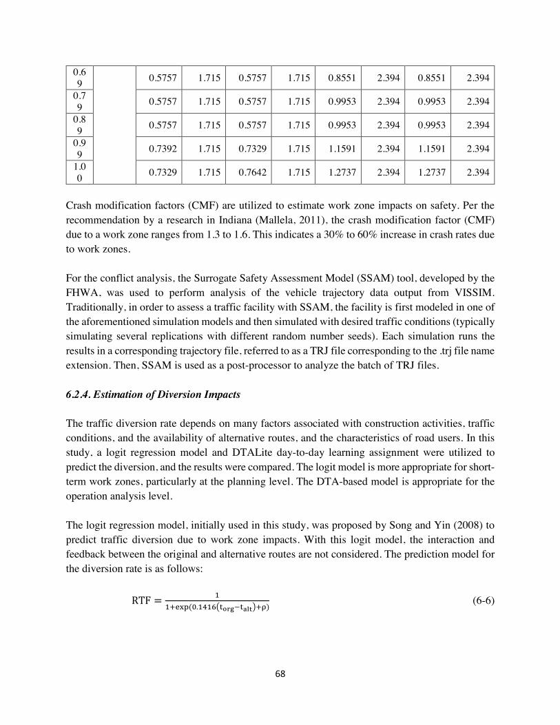
68

0.69 0.5757 1.715 0.5757 1.715 0.8551 2.394 0.8551 2.394

0.79 0.5757 1.715 0.5757 1.715 0.9953 2.394 0.9953 2.394

0.89 0.5757 1.715 0.5757 1.715 0.9953 2.394 0.9953 2.394

0.99 0.7392 1.715 0.7329 1.715 1.1591 2.394 1.1591 2.394

1.00 0.7329 1.715 0.7642 1.715 1.2737 2.394 1.2737 2.394

Crash modification factors (CMF) are utilized to estimate work zone impacts on safety. Per the recommendation by a research in Indiana (Mallela, 2011), the crash modification factor (CMF) due to a work zone ranges from 1.3 to 1.6. This indicates a 30% to 60% increase in crash rates due to work zones. For the conflict analysis, the Surrogate Safety Assessment Model (SSAM) tool, developed by the FHWA, was used to perform analysis of the vehicle trajectory data output from VISSIM. Traditionally, in order to assess a traffic facility with SSAM, the facility is first modeled in one of the aforementioned simulation models and then simulated with desired traffic conditions (typically simulating several replications with different random number seeds). Each simulation runs the results in a corresponding trajectory file, referred to as a TRJ file corresponding to the .trj file name extension. Then, SSAM is used as a post-processor to analyze the batch of TRJ files. 6.2.4. Estimation of Diversion Impacts The traffic diversion rate depends on many factors associated with construction activities, traffic conditions, and the availability of alternative routes, and the characteristics of road users. In this study, a logit regression model and DTALite day-to-day learning assignment were utilized to predict the diversion, and the results were compared. The logit model is more appropriate for short-term work zones, particularly at the planning level. The DTA-based model is appropriate for the operation analysis level. The logit regression model, initially used in this study, was proposed by Song and Yin (2008) to predict traffic diversion due to work zone impacts. With this logit model, the interaction and feedback between the original and alternative routes are not considered. The prediction model for the diversion rate is as follows:

RTF = ++8!m? (@.+n+op$qLrs$tuNv8w) (6-6)

69

Where, tx y and t2<$ are the travel times of original and alternative routes, respectively. ρ is the model parameter that was calibrated based on work zone location and weather, shown in Table 6-5. Table 6-5 Value of Parameter Í

Parameter Value Work Zone Location Rural Urban

Weather Condition Normal -0.6166 0.1054 Bad -0.2207 0.5013

A new logit model was developed in this study that considers day-to-day learning based on DTALite by including the number of the days that the work zone was active as an independent variable in the regression. Thus, this model considers the interactions with the alternative routes. However, this model is developed based on a single network (the I-595 network). Thus, DTA utilization is necessary to ensure accurate estimation of the diversion. For the operation level, the day-to-day learning traffic assignment option of DTALite was used for the analysis. In this study, the diversion is estimated by tracking the vehicles that travel from origins to destinations using the link-based results reported in the DTALite output. Figure 6-6 illustrates the work zone and alternative route used by the DTALite assignment for an Origin-Destination Pair.

Figure 6-6 Original Route and Alternative Route of Work Zone Used by DTALite

Assignment for an O-D Pair Notes: The squares in figure above represent the origin and destination of the O-D pair. The blue link represents the original route, while the pink link represents the alternative route. 6.2.5. Estimation of Reliability Impacts

70

This study uses regression equations to estimate reliability for both the planning level and operation level analyses. These equations were originally developed in the SHRP 2 L03 project (Cambridge Systematics, 2011). The simulation-based reliability estimation of SHRP 2 L04 can be used for more detailed operation studies. This procedure was not performed in this study. The utilized measures of reliability that can be calculated using the models are the nth percentile travel time indexes (TTIs), where nth could be the 10th, 50th, 80th, 95th, and mean travel time index (TTI). The TTI estimation models have the following general functional form:

TTI.% = e(FGHIH8JG4#KLMN8<GOP.PQ") (6-7) Where, TTI.% represents the nth percentile TTI. LHL represents the lane hour lost. dc# "$ represents the demand-capacity ratio. R@.@U" represents the hours of rainfall exceeding 0.05 of an inch, and j., k.,l. represents the coefficients for nth percentile TTI. In order to convert the reliability into a dollar value, it is necessary to estimate the value of reliability (VOR). The L04 project of the SHRP 2 program (Mahmassani et al., 2014) recommended that the VOR value is set as a function of the travel purpose, household income, car occupancy and travel distance. In this study, the buffer time, representing the extra time budgeted for travel, is selected as the reliability measure to estimate reliability costs based on its use in the SHRP 2 L04 project, as follows:

ReliabilityCosts = VOR ∗ BufferTime (6-8) BufferTime = Vehicles ∗ Occupancy ∗ AveTravelTime ∗ (™U%êê§sä!4"2.êê§)

ä!4"2.êê§ (6-9) Where, the VOR value used in this project is 22.5$/hr, according to the SHRP 2 L04 project. BufferTime defines the additional amount of time needed to be on time. Vehicles represents the number of vehicles in the study period. Occupancy represents the average occupancy for automated vehicles. AveTravelTime represents the average travel time for drivers to pass the work zone area. TTI represents the Travel Time Index. 6.2.6. Estimation of Emission Impacts Work zone can also increase pollutant emissions from vehicles due to the increase in stops and decrease in speed. The average speed approach of the Motor Vehicle Emission Simulator (MOVES) (EPA, 2010), developed by the United States Environmental Protection Agency (EPA), was used in this study to estimate emission. The average speed approach is the simplest of the project level analysis in MOVES and is based on the average speed of the vehicles and the vehicle miles traveled by vehicle type. Figure 6-7 displays the emission rates used in this study.

71

Figure 6-7 Emission Rates of Pollutants

The emission cost was then estimated using the following equation:

EmissionCost = UnitCost ∗ VMT ∗ EmissionRate(PollutantType, Speed) (6-10) Where, the utilized unit costs of emissions were obtained from the FHWA work zone road user cost manual mentioned earlier (FHWA, 2011). Three types of pollutants are considered in this study: Carbon Oxide (CO), Nitrogen Oxide (NOx), and Hydrocarbons (HC). 6.3. Microscopic Simulation Model Preparation To investigate the impacts of a work zone and associated strategies considering the detailed driving behaviors, VISSIM, which is a microscopic, stochastic, discrete time-step-based simulation tool, was utilized to conduct a more detailed level of analysis in conjunction with DATlite. As such, DTALite provides the strategic diversion behaviors of drivers, while VISSIM provides the mobility and microscopic traffic behavior impacts. VISSIM has two car-following models: Wiedemann 74 and Wiedemann 99, and a lane-changing model. The Wiedemann 99 car-following model represents freeway condition, and there are ten user-defined driving behavior parameters, CC0, CC1, …, CC9, which classify driving behavior. The lane-changing model in VISSIM is based on the driver’s response to the perception of the surrounding traffic. Necessary lane changes depend on the aggressiveness of drivers in accepting/rejecting gaps in adjacent lanes. The safety reduction factor (SRF) defines the reduction in safety distance for lane changing. A lower SRF value, for instance 0.4, means that the safety distance for lane changing is reduced by 60%, which suggests that drivers are more aggressive in accepting shorter gaps. Table 6-6 describes the parameters that influence car-following and lane-changing behaviors in VISSIM. Table 6-6 Parameter Range and Default Value

Parameter Description Default value Range

72

CC0 Standstill distance between two stopped vehicle

4.92ft

CC1 Desired time headway 0.9sec 0.9~1.8sec CC2 Following variation 13ft 10~55ft CC3 Threshold for entering “Following” -8.00 CC4 Following threshold -0.35 CC5 Following threshold 0.35 CC6 Speed dependency 11.44 CC7 Oscillation acceleration 0.82ft/s2 0.4~2.0ft/s2 CC8 Standstill acceleration 11.48ft/s2 CC9 Acceleration at 80 km/h 4.92ft/s2 SRF Safety distance reduction factor 0.6 0.15~0.6

Gomes et al. (2004) utilized the CC0, CC1 and CC4/CC5 pairs to calibrate the value of field capacity in their VISSIM simulation study. The CC0 value was changed globally from 1.5 to 1.7 seconds, and this parameter was used specifically to calibrate the queue length, as it has more significance at lower speed conditions. The overall selection of the parameter values was done manually and based on the visual interpretation of the results. Lownes et al. (2006) performed an analysis of the quantitative impact of VISSIM driving behavior parameters in estimating capacity. The impacts of the Weidman 99 driving behavior parameter and lane-changing distance were investigated. Each of the ten behavior parameters were tested at four levels, namely “low,” “medium,” “calibrated” and “high,” depending on the values selected for each parameter. The results suggested that parameter CC0 produced significant differences only when the CC0 value is at a high level, but the CC1 values at all four levels resulted in a significant difference in the simulated capacity. Similarly for CC2, as its value increased, a drop in the mean value of capacity was observed. As mentioned earlier, the work zone capacity values that were estimated using the HCM and NCHRP’s project 03-107 methods were used to calibrate the driving behavior parameters in VISSIM. Only four parameters were selected for use in the calibration, based on the findings from previous studies. These parameters are CC0, CC1, CC2, and SRF. After the calibration, the resulting simulated capacity value was 1,880 vphpl for normal freeway, 1,144 vphpl for the 3-to-1 lane work zone, and 1,290 vphpl for the 4-to-2 lane work zone. When compared with the work zone capacity value range in Section 3.2.1, which is 1000 to 1300 vphpl for the 3-to-1 lane work zone and 1,200 to 1500 vphpl for the 4-to-2 lane work zone, the VISSIM calibration is acceptable. Table 6-7 presents the selected parameter. Table 6-7 Selection of Parameter

Parameter Default Value Range Calibration Value CC0 4.92ft - 4.92ft CC1 0.9sec 0.9-1.8sec 1.1sec CC2 13.2ft 10-55ft 25ft SRF 0.6 0.15-0.6 0.6

73

6.3. Monetary and Non-Monetary Evaluation Traditionally, economic analysis, such as present worth or benefit-cost analyze, has been utilized to assist decision makers in evaluating and comparing one or more alternatives to a “base case” of construction projects. In this study, the performance measures estimated in the previous module will be converted into dollar values and used as road user costs in the life cycle cost analysis. Construction costs, including both direct and indirect costs that are used as inputs to the analysis, will be estimated using models developed by researchers in the Construction Management Department at Florida International University. Smart zone strategies will also be estimated and used in the analysis. The present worth analysis (PWA) is then calculated based on construction and user costs in the current period, and then added to the initial costs to determine the PWA. In addition to the PWA estimation as a decision support method, MCDM was used in this study to capture all quantity and quality impacts and account for stakeholder preference. In this study, the TOPSIS MCDM is used for selecting between construction and operation strategy alternatives. The results from using the MCDM and PWA for the planning and operation analysis levels are then compared. The following are steps on how to apply the TOPSIS procedure:

• Step 1: Calculation of the Synthetic Importance Weight Matrix. This calculation involves asking decision makers, using linguistic variables, to express their perceptions of the level of importance of each criterion. This will allow for the calculation of an integrated fuzzy importance weight matrix for the valuing criteria.

• Step 2: Building the Fuzzy Decision Matrix. This step involves decision makers using linguistic terms to express their opinions about the rating of every alternative based on the raw data provided.

• Step 3: Calculating Weighted Normalized Fuzzy Decision Matrix. Considering the weights and the ratings of each alternative, the weighted normalized fuzzy decision matrix will be obtained using the matrix produced in Step 1 and Step 2.

• Step 4: Calculating the Performance of Each Alternative Using the Closeness Coefficient (CC). The closeness coefficient is measured using the Euclidean distances of each candidate system to the fuzzy positive ideal solution and the fuzzy negative ideal solution.

The fuzzy TOPSIS MCDM method described earlier was utilized for the selection between the construction and work zone alternatives using accelerated bridge construction (ABC) technology and smart work zone strategy for the I-4 and I-595 construction projects. There are five criteria included in the evaluation:

74

C1: Mobility Costs C2: Reliability Costs C3: Safety Costs C4: Emission Costs C5: Construction Costs In this study, the triangular fuzzy number is utilized to express the importance of each criteria and assessment of each alternative. The linguistic variable for the importance of each criteria ranges from “very low” to “very high,” and the linguistic variable for the assessment of each alternative ranges from “very poor” to “very good.” The linguistic variable has seven grades, which are shown in Table 6-8 and Table 6-9, based on an input from an input from an experienced previous state department of transportation engineer. In real-time implementation of this method, these weights should be assigned by project stakeholders. Table 6-8 Linguistic Variables for the Importance Weight of Each Criteria

Linguistic Variable Corresponding Triangular Fuzzy Number Very Low (VL) (0,0,0.1)

Low (L) (0,0.1,0.3) Medium Low (ML) (0.1,0.3,0.5)

Medium (M) (0.3,0.5,0.7) Medium High (MH) (0.5,0.7,0.9)

High (H) (0.7,0.9,1.0) Very High (VH) (0.9,1.0,1.0)

Table 6-9 Linguistic Variable for Rating

Linguistic Variable Corresponding Triangular Fuzzy Number Very Poor (VP) (0,0,1)

Poor (P) (0,1,3) Medium Poor (MP) (1,3,5)

Fair (F) (3,5,7) Medium Fair (MG) (5,7,9)

Good (G) (7,9,10) Very Good (VG) (9,10,10)

Decision makers could use the linguistic variable to express their perceptions about the level of importance of each criteria and assessment of each criteria based on the linguistic variable table mentioned above. Table 6-10 shows the importance of criteria based on expert survey data.

75

Table 6-10 Criteria Importance Table Criteria Expert1 Expert2 Expert3 Expert4

C1:Mobility H VH VH H C2:Reliability H VH MH ML

C3:Safety VH VH H H C4:Emission M MH MH L

C5:Construction Costs VH H H VH For the assessment of each alternative, it is not necessary to convert all of the performance measures to dollar value. Thus, the performance measure will keep its unit in the fuzzy evaluation. The evaluation index selected for each criterion is listed as: total travel delay (mobility), TTI (reliability), number of conflicts (safety), pollutants weight (emission), implementation and maintenance costs (construction). To make the ratings for each criterion more flexible and understandable, the performances of alternative traffic management scenarios, which are Accelerated Bridge Construction (ABC) and conventional method, were compared. The increasing/decreasing percentage of the performance measures using the ABC method compared to that of using the conventional method was utilized to determine the rating for each criterion. Through the expert survey, the rating principle of performance ABC with respect to Conventional Construction was shown in Table 6-11. Users can provide the ratings based on the rating principle and their own experience. Table 6-11 Rating of the Performance of ABC with Respect to Conventional Construction

Rating Expert Mobility Impacts

Reliability Impacts

Safety Impacts

Emission Impacts

Construction Costs

VP

Expert1 Expert2 Expert3 Expert4

Equal or higher Equal or higher

10% lower 10% higher

Equal or higher Equal or higher

10% lower 10% higher

Equal or higher Equal or higher

10% lower 10% higher

Equal or higher Equal or higher

10% lower 10% higher

100% higher 10% higher 50% higher

30% higher

P

Expert1 Expert2 Expert3 Expert4

10~30% lower 0~10% lower

10~20% lower 0~10% higher

10~30% lower 0~10% lower

10~20% lower 0~10% higher

10~30% lower 0~10% lower

10~20% lower 0~10% higher

10~30% lower 0~10% lower

10~20% lower 0~10% higher

75~100% higher 5~10% higher

40~50% higher 25~30% higher

MP

Expert1 Expert2 Expert3 Expert4

30~45% lower 10~15% lower 20~35% lower

0~15% lower

30~45% lower 10~15% lower 20~35% lower

0~15% lower

30~45% lower 10~15% lower 20~35% lower

0~15% lower

30~45% lower 10~15% lower 20~35% lower

0~15% lower

50~75% higher 0~5% higher

35~40% higher 20~25% higher

F

Expert1 Expert2 Expert3 Expert4

45~60% lower 15~20% lower 35~50% lower 15~30% lower

45~60% lower 15~20% lower 35~50% lower 15~30% lower

45~60% lower 15~20% lower 35~50% lower 15~30% lower

45~60% lower 15~20% lower 35~50% lower 15~30% lower

30~50% higher Equal

30~35% higher 15~20% higher

MF

Expert1 Expert2 Expert3 Expert4

60~80% lower 20~30% lower 50~65% lower 30~45% lower

60~80% lower 20~30% lower 50~65% lower 30~45% lower

60~80% lower 20~30% lower 50~65% lower 30~45% lower

60~80% lower 20~30% lower 50~65% lower 30~45% lower

20~30% higher 0~5% lower

20~30% higher 10~15% higher

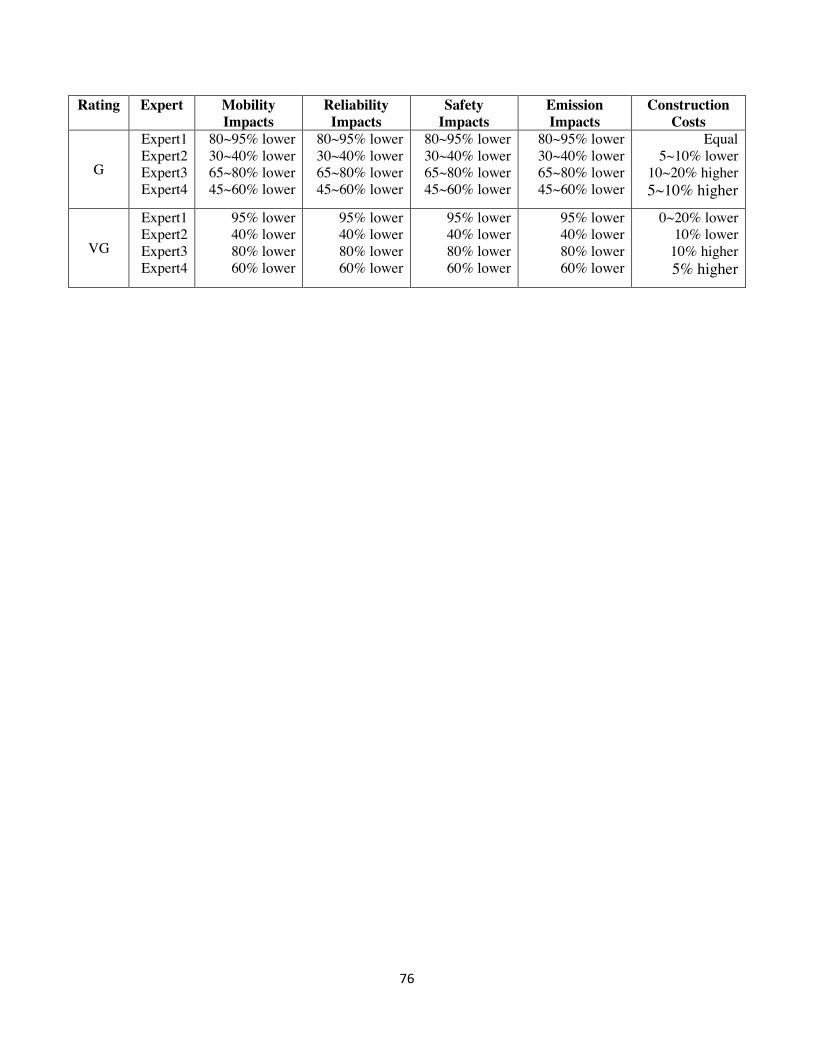
76

Rating Expert Mobility Impacts

Reliability Impacts

Safety Impacts

Emission Impacts

Construction Costs

G

Expert1 Expert2 Expert3 Expert4

80~95% lower 30~40% lower 65~80% lower 45~60% lower

80~95% lower 30~40% lower 65~80% lower 45~60% lower

80~95% lower 30~40% lower 65~80% lower 45~60% lower

80~95% lower 30~40% lower 65~80% lower 45~60% lower

Equal 5~10% lower

10~20% higher 5~10% higher

VG

Expert1 Expert2 Expert3 Expert4

95% lower 40% lower 80% lower 60% lower

95% lower 40% lower 80% lower 60% lower

95% lower 40% lower 80% lower 60% lower

95% lower 40% lower 80% lower 60% lower

0~20% lower 10% lower

10% higher 5% higher

77

7. APPLICATION OF MULTI-CRITERIA EVALULATION FRAMEWORK The decision-making analysis framework and the associated analysis described in the previous section were applied to the I-4 and the I-595 case studies. The planning level decision making analysis was conducted for both case studies, while the operational analysis was only applied to the I-595 case study, since there is no detailed traffic network data for the I-4 case study. This section describes the results obtained from the implementation of the two case studies. 7.1. I-4 at Graves Avenue Interchange Case Study This case study represents a three-mile work zone located along the I-4 corridor near the Graves Avenue Interchange in Orlando, Florida. The duration of the work zone activities was assumed to be three hours each day, and two out of the facility’s three lanes were closed during construction. The construction zone segment has an AADT of 67,000 vehicles per day (see Figure 7-1). During construction, an existing two-lane four-span concrete beam bridge was widened to 33 feet with two traffic lanes, a shoulder and a sidewalk on each side. The basic information for this project is shown in Table 7-1.

Figure 7-1 Location of Study Bridge Construction Project

Table 7-1 Basic Information for I-4/Graves Bridge

78

Segment No. of Lanes Length (miles) Free-flow speed (mph) I-4-work zone 3 lanes 3.11 60 Detour for I-4 2 lanes 4.32 30 Graves Ave 1 lane 0.83 45

Detour for Graves 1 lane 1.91 30 The decision support framework described in the previous section is applied to this case study to select between conventional construction and accelerated bridge construction (ABC). Only the planning level approach to estimate the performance measures is used in this case. Both approaches (the planning and operations approaches) are used in the analysis of the second case study, discussed in the next section. The construction period and lane closure schedules are different between the ABC and the conventional construction methods. The associated in the construction costs, user costs, and thus the total costs are different between the two construction approaches and must be estimated and compared. Following are the estimated construction durations for the different alternatives. • ABC Method. The ABC Method requires I-4 to close one outside lane from 21:00 to 24:00

for only four nights. This schedule was obtained based on project documents. • Conventional Method I. Conventional Method I requires I-4 to close two outside lanes from

21:00 to 24:00 for 48 nights. This schedule is a hypothetical schedule identified in this study as a potential variation for Conventional Method II identified in project documents. The main purpose for including this additional method, although not specified as an option in the project document, is to further the comparison that can be made using the identified framework. Due to the site overhead costs caused by the longer period of Conventional Method I compared to Conventional Method II, the construction cost of Method 1 is assumed to be 15% higher than the Conventional Method II.

• Conventional Method II. Conventional Method I requires I-4 to close all lanes from 21:00

to 24:00 for 32 nights. This is a schedule obtained from the project documentation that shows the schedule of the construction estimated by the agency for the conventional bridge construction.

Work zone capacity has a large influence on the estimation of mobility and reliability impacts and thus the road user costs. Since there is uncertainty in the open-lane capacity during construction, sensitivity analysis was done to determine the impact of this parameter value on the analysis results. In this study, three values of work zone capacity were utilized and the results of the analysis were compared to determine the impacts on the analysis results: an estimate from a previous analysis of real-world data by this study’s researchers (capacity equal to 1000 veh/hr/lane), a HCM 2010 methodology (1136 veh/hr/lane), and a method presented in the NCHRP project 03-107 report (capacity equal to 1264 veh/hr/lane).

79

Another important issue is the route diversion due to construction zones. During the lane closure period, drivers may choose to divert to alternative routes. The logit model developed by Song and Yin (2008) as reviewed earlier was utilized to estimate traffic diversion. As a result, a 15.8% diversion rate was utilized for both one-lane closure and two-lane closure, and a 100% diversion to the alternative route for the full-lane closure. The results from applying the framework to the case study are shown in Table 7-2 and Figures 7-2 to 7-4. As shown in Figure 7-2, the construction cost of the ABC is higher than that of the conventional method according to the utilized construction cost estimation method. This could be in part due to the lesser amount of experience with ABC compared to the conventional methods, raising the possibility of the ABC costs decreasing with the increasing experience of ABC. The Conventional Method I (Con I in the Table 7-2) has a 15% higher construction cost compared to Conventional Method II (Con II in the Table 7-2) due to the longer construction period. If the comparison was based on the construction cost alone, agencies would select Conventional Method II. This illustrates the importance of considering the user impacts, in addition to user costs in the analysis. The Quick Zone sketch planning tool was used to estimate the mobility impacts. As shown in Table 7-2, the ABC method has the lowest mobility impacts. Conventional Method II has the highest impacts since all of the vehicles had to use an alternative route with the full closure required by this method. The reliability, emission, and safety impacts are also shown in Table 7-2 and Figures 7-2 to 7-4. If the mobility (travel time delays due to construction) is added to the comparison, as is sometimes done when comparing construction and construction management alternatives, Figure 7-3 shows that Conventional Method II becomes the alternative with the highest cost. However, the cost of Conventional Method I is still lower than the ABC cost, as shown in Figure 7-3. When all components of the user costs are added to the analysis, ABC became the best alternative in Figure 7-4, except for the optimistic lane capacity of the work zone (capacity of 1264 veh/hr/lane). This illustrates the benefit of using the total costs, which includes the user costs, in the comparison with ABC and conventional methods. If additional user costs, such as the impacts on businesses and toll revenue losses, if any, could be added, then the user costs would be even higher. In this project, I-4 was not a tolled highway, and there were no impacts on businesses that could be quantified. Table 7-2 Total Costs for Different Alternatives

Costs in dollar value ($) Mobility Costs

Reliability Costs

Safety Costs

Emission Costs Construction Construction

Agency Costs Total Cost

C=1000 veh/hr/lane

ABC 120,347 32,807 40,864 1,615 430,000 53,320 678,953 Con I 224,591 258,414 77,313 2,274 342,125 46,529 951,246 Con II 487,838 258,580 127,434 3,102 297,500 40,460 1,214,914

C=1136 veh/hr/lane

ABC 120,347 32,489 40,864 1,615 430,000 53,320 678,635 Con I 191,339 202,851 77,207 2,425 342,125 46,529 862,476

80

Con II 487,838 258,580 127,434 3,102 297,500 40,460 1,214,914 C=1264

veh/hr/lane ABC 120,347 32,311 40,864 1,615 430,000 53,320 678,457 Con I 183,026 73,715 77,207 2,499 342,125 46,529 725,101 Con II 487,838 258,580 127,434 3,102 297,500 40,460 1,214,914

Figure 7-2 Comparison of Construction Costs

Figure 7-3 Comparison of the Construction Costs When Mobility Costs is Added

81

Figure 7-4 Comparison of the Total Costs of Different Alternatives

The fuzzy TOPSIS approach was also conducted for the evaluation between ABC and conventional construction alternatives. As described earlier, the performance measure does not require conversion to a dollar value, as shown in Table 7-3 (1136 veh/hr/lane used as work zone capacity). Based on the fuzzy evaluation approach described in the previous section, the performance measures were rated to linguistic variable according to the rating principle, as shown in Table 7-4. Table 7-3 Comparison of Different Alternatives

Scenario Mobility Impacts

(In veh.hr)

Reliability Impacts

(In veh.hr)

Emission Impacts (In ton)

Safety Impacts

(Crashes)

Construction Costs (Direct and Indirect)

ABC 7,338 1,444 2.79 0.79 483,320 CONI 11,667 9,016 4.19 1.49 388,654 CONII 29,746 11,492 5.36 2.46 337,960 No Work Zone 0 848 1.64 0.54 0

82

Table 7-4 Rating Results for Alternatives

Alternatives Mobility Impacts

(In veh.hr)

Reliability Impacts

(In Veh.hr)

Emission Impacts (In ton)

Safety Impacts

(Crashes)

Construction Costs (Direct and Indirect)

User1 ABC VG VG G VG MP CONI G MP MP F MF CONII P VP P P G

User2 ABC VG VG VG VG P CONI G F F F P CONII VP VP VP VP VG

User3 ABC VG G F VG VP CONI F MP VP MF MF CONII VP VP VP VP VG

User4 ABC VG G VG VG MG CONI MP F P G G CONII VP VP VP VP G

Combined with the criteria importance in Table 6-9, the fuzzy evaluation results are listed in Table 7-5. D(max) represents the distance between the alternative to the best alternative, while D(min) represents the distance between the alternative to the worst alternative. CC shows the ranking of alternatives. It can be found that the ABC alternative has a significant advantage in implementation when compared to other alternatives. This result is consistent with that of the present worth analysis. Table 7-5 Fuzzy Evaluation Results

Alternatives D(max) D(min) CC ABC 3.076 6.178 0.667

Con(2) 5.993 3.029 0.335 Con(3) 7.036 1.929 0.215

83

7.2. I-595 Corridor Case Study This case study was used to illustrate the use of both the planning level and operation level analyses for a more congested urban environment. The case study was conducted for a construction project along the I-595 corridor in Broward County, Florida. Assessment of accelerated construction and operation smart work zone strategy impacts will be conducted using the analysis methods. A particular emphasis is placed on estimating strategic driver behaviors in terms of diversion and microscopic behavior in terms of lane changing ahead of the work zone. 7.2.1 Traffic Diversion Analysis Three methods of diversion estimation during construction were examined in this study: 1) diversion during short-term construction utilizing a logit model developed in a previous study（Song and Yin，2008); 2) diversion during long-term construction where the network reaches user equilibrium (modeled using the MSA (Method of Successive Average) option in DTALite); and 3) diversion through a day-to-day learning assignment in DTA modeling that accounts for the number of days that the construction zone is active (modeled using a day-to-day learning assignment in DTALite). A regression model was developed in this study based on the results from the DTALite to facilitate the estimation of diversion when there are limited resources for the effort that do not allow a DTA to be conducted(Dynamic Traffic Assignment). In this study, a construction zone was assumed to be located along I-595 westbound in Broward County, Florida. The travel demand from the Port Everglades zone (ZONE ID: 147) to I-595 Westbound (ZONE ID: 165) was analyzed. Figure 7-5 shows the location of the construction zone and its main alternative route (SR 84). The corresponding lengths and free-flow travel times for these two paths are summarized in Table 7-6.

84

Figure 7-5 Location of Work Zone and Alternative Route

Table 7-6 Basic Information of Travelling Paths in the Case Study

From Zone To Zone Path Length (mile) Free-Flow Travel Time (min) 147 165 I-595 6.6 8.58 147 165 SR-84 6.4 11.03

Four scenarios were considered in this study, as follows: • Scenario 1: Simulation is conducted for 100 days without a work zone, which is a base case

for comparison. • Scenario 2: Simulation is conducted for 100 days with a work zone using the MSA method. It

is assumed that the system reaches user equilibrium in case of long-term work zones. • Scenario 3: Simulation is conducted for 100 days with a work zone using the day-to-day

learning assignment method, and then observing the change in diversion behaviors when increasing the number of days of the work zone.

• Scenario 4: The logit regression model developed by Song et al. (2008) is also utilized to estimate traffic diversion.

Figures 7-6 displays the results of the traffic diversion estimation using different methods. As shown in the figure, both the MSA method and day-to-day learning method produce similar results after 100 days of learning as the traffic assignment reaches equilibrium in both cases. In equilibrium, about 50 percent of the vehicles shift to other routes. In short-term work zones, as modeled using day-to-day learning, 50% of the traffic is diverted to alternative routes due to the severity of the work zone blockage (resulting in demand/capacity ratio of 2.5). However, in the short-term modeling of the work zone (three days), the day-to-day learning indicates the overreaction of drivers to the work zone, with about 60% of the traffic diversion. This overreaction

85

appears to result in overloading alternative routes, resulting in a proportion of these vehicles returning to the original path where the work zone occurs. The logit model by Song et al. (2008) estimates only 28%. It should be noted that this logit model does not account for the severity of the work zone lane blockage and the associated delays. An attempt was made to fit a logit model based on the DTALite day-to-day learning traffic assignment. The model estimates the diversion based on the demand/capacity ratios on the work zone link and the alternative route and the number of work zone days. The expression is shown as follows:

Diversion Rate = +(+8!(t∗¥µLtNMqÖ×∗ØtÙÚÖK∗ªKLtNMqºÖØ∗ØtÙÚºÖÝ∗¥µLtNMq∗ØtÙÚÖæ)) (7-1)

Where, Diversion Rate defines the percentage of the vehicles diverted. The DCratio represents the demand/capacity ratios on the work zone link. and days represents the number of work zone days. The a, b, c, d, e and f represent the coefficients. In order to build the regression model to estimate diversion, multiple runs of DTALite were conducted with a different number of days and demand/capacity ratios. The results are shown in Table 7-7. Table 7-7 DTALite Results for Diversion Analysis

Number of Days Demand/Capacity Ratio

Number of Vehicles Stay at Original Route

Diversion Percentage

10 3.75 1751 71% 15 3.75 1999 67% 25 3.75 2165 64% 50 3.75 2280 62%

100 3.75 2251 62% 10 3.00 2016 66% 15 3.00 2358 61% 25 3.00 2682 55% 50 3.00 2601 57%

100 3.00 2561 57% 10 2.50 2458 59% 15 2.50 2656 56% 25 2.50 2996 50% 50 2.50 2776 54%

100 2.50 2829 53% 10 2.14 2465 59% 15 2.14 2921 51% 25 2.14 3293 45% 50 2.14 3021 50%

86

Number of Days Demand/Capacity Ratio

Number of Vehicles Stay at Original Route

Diversion Percentage

100 2.14 2976 50% 10 1.88 2465 59% 15 1.88 3229 46% 25 1.88 3541 41% 50 1.88 3190 47%

100 1.88 3353 44% 10 1.50 2465 59% 15 1.50 3239 46% 25 1.50 4140 31% 50 1.50 3990 34%

100 1.50 3996 33% 10 1.00 2465 59% 15 1.00 3206 47% 25 1.00 4382 27% 50 1.00 4516 25%

100 1.00 4716 21% SPSS was utilized to conduct the regression analysis. Through regression analysis, the significant parameters, which are DCratio, days and DCratio*days, were kept in the regression model. The R-square for the regression model is 0.501. The t statistics of the three parameters is significant at the 0.05 confidence level, as shown in Table 7-8. However, it appears that particularly for short-term work zones, the DTALite day-to-day learning model overestimated the diversion significantly, as shown in Figure 7-6. Thus, using the day-to-day learning and the model developed based on it without considering the number of drivers willing to divert does not produce a good estimate of the diversion. Table 7-8 Parameter Estimates

Parameter Estimate Std. Error

95% Confidence Interval t Sig. Lower

Bound Upper Bound

a (DCratio) -0.268 0.052 -0.373 -0.164 -5.153 0.000 b (days) 0.021 0.006 0.010 0.033 3.333 0.001 e (DCratio*days) -0.005 0.002 -0.009 1.228E-005 -2.500 0.003

87

Figure 7-6 Comparison of Diversion Percentage Estimates Using Different Approaches

For this reason, the dynamic user equilibrium of DTALite using the MSA traffic assignment, was used to produce another logit regression model based on the Demand/Capacity ratio at the work zone link without considering the duration of the work zone. The expression is shown as follows:

Diversion Rate = +(+8!(t∗¥µLtNMqÖ×∗ªKLtNMqºÖK∗uG (¥µLtNMq)ÖØ)) (7-2)

where Diversion Rate defines the percentage of the vehicles diverted. The DCratio represents the demand/capacity ratios on the work zone link. The a, b, c and d represent the coefficients. The R-square for the regression model is 0.980. The t statistics of the three parameters is significant at the 0.05 confidence level, as shown in Table 7-9. When compared with the logit regression model developed by Song et al. (2008), which does not consider the D/C ratio impact on diversion, the diversion percentage varies from 20% to 60% with the model in Equation 7-3. Table 7-9 Parameter Estimates

Parameter Estimate Std. Error

95% Confidence Interval t Sig. Lower

Bound Upper Bound

a (DCratio) -1.415 0.175 -1.788 -1.041 -8.086 0.000 b (DCratio2) 0.177 0.042 0.089 0.266 4.214 0.000 e (Constant) 2.354 0.169 1.992 2.715 13.929 0.000

0%

10%

20%

30%

40%

50%

60%

70%

80%

10 30 50 70 90

Dive

rsio

n Pe

rcen

tage

No of days

Diversion at I595 Work Zone (MSA Method)Diversion at I-595 Work Zone (Day-to-day learning)Diversion at I-595 Work Zone (Logit Model)Diversion at I-595 Work Zone (New Model)

88

Figure 7-7 Comparison of Diversion Percentage Estimates Using Different Approaches

7.2.2. Microscopic Lane Merging Behavior Lane merging behavior was investigated utilizing the VISSIM microscopic simulation modeling. As stated earlier, the lane-changing distance in the connectors controls the drivers’ lane-changing behaviors by forcing the drivers to change lanes before the connector link. Current lane merging enhancement strategies at work zones include late merge and early merge. Generally, the late merge strategy could fully use the capacity of closed lanes until the work zone taper area; however, this would induce the increase of potential conflicts due to late merging behavior. On the other hand, the early merge strategy could guide drivers’ lane-changing behaviors by merging early, but would increase the queue length of open lanes. This section aims to investigate the optimal lane-changing distance to improve the mobility and safety impacts at work zones. This distance can be achieved as a connected and automated vehicle application. The network utilized is the I-595 corridor described earlier, and an assumed work zone was built based on the construction activities along the I-595 corridor in Broward County, Florida. The work zone was 1.5-miles long and had a 4-to-2 lane configuration. Detailed information is shown in Table 7-10, and the corresponding VISSIM configuration is shown in Figure 7-7. Table 7-10 Basic Information of I-595 Work Zone

Location Length (miles)

FFS (mph)

Lane Closure Schedule

Working Activity Schedule

I-595, Broward 1.5 65 2 out of 4 lanes 3:30~6:30

0.00%

10.00%

20.00%

30.00%

40.00%

50.00%

60.00%

70.00%

0.5 1 1.5 2 2.5 3 3.5

Dive

rsio

n Pe

rcen

tage

Demand/Capacity Ratio

Diversion at I-595 Work Zone (MSA Method)

Diversion at I-595 Work Zone (Logit Model)

Diversion at I-595 Work Zone (New Model)

89

Figure 7-8 I-595 Work Zone in VISSIM

In order to optimize the lane-changing distance parameter, multiple work zone scenarios utilizing different lane-changing distances were built ranging from 200 feet to 2,000 feet. Travel delay, queue length and number of conflicts are the three performance measures that were used to compare the lane-changing distance parameter. The capacity resulting from each merging scenario and the vehicle trajectory distribution resulting from each distance in VISSIM were also obtained and were related to each other. In terms of the randomness of simulation, five simulation runs using different seed numbers were conducted for each work zone scenario. The comparison results are shown in Table 7-11. Table 7-11 Performance of Each Work Zone Scenario Lane-changing

Distance Group(ft)

Seeds Number

Average Travel Delay

(sec) Average Queue

length (ft) Number of Conflicts

Work Zone Throughput

(vph)

2000

55 377.56 4711 26450 2380 65 372.8 4635 26416 2413 75 404.5 5171 28189 2270 85 385.17 4839 25712 2395 95 329 4208 24556 2410

1600

55 407.43 5168 28501 2385 65 396.69 4819 26937 2364 75 363.19 4520 27020 2331 85 377.4 4734 25609 2349 95 311.7 4057 23565 2440

1300

55 370.3 4442 25882 2451 65 330.2 4164 25479 2362 75 391.6 4877 27577 2418

90

Lane-changing Distance

Group(ft) Seeds

Number Average

Travel Delay (sec)

Average Queue length (ft)

Number of Conflicts

Work Zone Throughput

(vph) 85 387.56 4651 25512 2381 95 304 3696 21673 2441

1000

55 424.2 5088 28209 2306 65 370.45 4351 25139 2350 75 387.41 4491 26998 2397 85 410.75 4781 26039 2387 95 279.9 3512 19976 2404

800

55 370 4233 24816 2377 65 372 4455 26666 2368 75 425 5062 28414 2317 85 392 4631 25602 2356 95 328 3880 23063 2415

500

55 389 4352 25563 2359 65 366.2 4336 25746 2313 75 423.7 4879 27892 2117 85 411.98 4794 26747 2275 95 332 3969 23838 2427

200

55 422 5011 28622 2321 65 461.81 5242 29721 2277 75 486.15 5628 30339 2195 85 424.25 5160 28116 2248 95 386.61 4562 27040 2252

Based on Table 7-11, the mean value of each group is compared and shown in Figures 7-9 to 7-12 below. It can be seen that the four performance measures increase dramatically when the lane-changing distance is lower than 800 feet. Most drivers decide to change lanes up until the work zone taper area, and the merging behavior reduces the travel speed and work zone capacity. On the other hand, four performance measures also increase when the lane-changing distance is higher than 1,300 feet. This occurs because the simulated drivers are guided to merge to open lanes earlier so that the queue length of the open lanes increases greatly. It can be concluded that the three performance measures have better performance when the lane-changing distance is between 1,000 feet and 1,300 feet.

91

Figure 7-9 Average Travel Delay

Figure 7-10 Average Queue Length

300

320

340

360

380

400

420

440

460

2000 1600 1300 1000 800 500 200

Dela

y(se

c)

Lane changing Distance (ft)

Travel Delay

3800

4000

4200

4400

4600

4800

5000

5200

2000 1600 1300 1000 800 500 200

Leng

th(ft

)

Lane Changing Distance (ft)

Queue Length

92

Figure 7-11 Average Number of Conflicts

Figure 7-12 Average Work Zone Throughput In order to verify better performance when the lane-changing distance is between 800 feet and 1,300 feet, the statistical t-test was utilized in this study. Generally, the t-test is used to determine if two sets of data are significantly different from each other. There are seven groups of data in this study in terms of the lane-changing distance. Since the traffic network and traffic demand are the same for all seven groups, the dependent paired sample t-test was conducted in this section. Similarly, the paired sample t-test was used when the samples were dependent, that is, when there was only one sample that was tested twice (repeated measures) or when there were two samples that were matched or "paired." The basic procedure is listed as follows:

23000

24000

25000

26000

27000

28000

29000

30000

2000 1600 1300 1000 800 500 200

No. o

f Con

flict

s

Lane changing Distance (ft)

Traffic Conflicts

2150

2200

2250

2300

2350

2400

2450

2000 1600 1300 1000 800 500 200

Vph

of tw

o la

nes

Lane Changing Distance

Work Zone Throughput

93

Let X and Y represent two paired samples. The t statistic can be calculated as follows:

t = ¿¡s¬¢¥

√.ƒ (7-3)

Where, D¡ represents the average difference of (X − Y). S¿ represents the standard deviation of these differences. n represents the sample size. In this study, three performance measures are compared: travel delay, queue length and number of conflicts. The t-test was conducted for each performance measure separately. Let L2000 represent the group with 2,000 feet of lane-changing distance specified in VISSIM, L1600 represents the group with a 1,600-foot distance, L1300 represents the group with a 1,300-foot distance, L1000 represents the group with a 1,000-foot distance, L800 represents the group with a 800-foot distance, L500 represents the group with a 500-foot distance, and L200 represents the group with a 200-foot. For travel delay, t statistics for the paired sample among seven groups are listed in Table 7-12, and Figure 7-13 shows a sample of the results. In order to compare the performance of each group, the one tail t-test was selected. The critical value is 1.533 at a 0.1 confidence level, according to the t-test table. It can be seen from Table 7-11 that group L3000 has the least amount of travel delays and is significantly lower than in groups L2000, L800, L500 and L200. Travel delays in group L1600 are significantly lower than in groups L800, L500 and L200. Travel delays for group L1000 are significantly lower than in group L200. Thus, the lane-changing distance ranging from 1,600 to 1,000 feet produce better travel delay performance.

Figure 7-13 Parts of the T-test Results

Table 7-12 T Statistics and P-value for Travel delay

94

T Statistics and P-value L2000 L1600 L1300 L1000 L800 L500 L200

L2000 0.191 (0.428)

2.198* (0.046)

-0.044 (0.483)

-0.749 (0.248)

-1.832* (0.070)

-6.286* (0.002)

L1600 -0.191 (0.428) 0.861

(0.219) -0.242 (0.410)

-0.350 (0.372)

-0.791 (0.237)

-3.647* (0.011)

L1300 -2.198* (0.046)

-0.861 (0.219) -1.248

(0.140) -2.541* (0.032)

-9.281* (0.000)

-4.765* (0.004)

L1000 0.044 (0.483)

0.242 (0.410)

1.248 (0.140) -0.153

(0.442) -0.649 (0.276)

-2.667* (0.028)

L800 0.749 (0.248)

0.350 (0.372)

2.541* (0.032)

0.153 (0.442) -1.363

(0.122) -6.340* (0.002)

L500 1.832* (0.070)

0.791 (0.237)

9.281* (0.000)

0.649 (0.276)

1.363 (0.122) -3.668*

(0.011)

L200 6.286* (0.002)

3.647* (0.011)

4.765* (0.004)

2.667* (0.028)

6.340* (0.002)

3.668* (0.011)

Note: * represents the significance at 0.1 confidence level. For queue length, similar to travel delay, a one-tailed test critical value of 1.533 at a 0.1 confidence level is utilized. Figure 7-14 shows a sample of the results. Table 7-13 presents the comparison of t statistics among seven groups. It should be noted that group L3000 has the shortest queue length and is significantly lower than the queues of the L2000, L1600, L500 and L200 groups. The queue length for group L1000 is significantly lower than the queues of the L1600 and L200 groups. Queue length for group L800 is significantly lower than in groups L2000 and L200. Thus, the lane-changing distance as specified in VISSIM, ranging from 1300 to 800, produce better queue length performance.

Figure 7-14 Parts of the T-test Results Table 7-13 T Statistics and P-value for Queue Length

95

T Statistics and P-value L2000 L1600 L1300 L1000 L800 L500 L200

L2000 0.287 (0.394)

5.597* (0.003)

1.330 (0.127)

4.020* (0.008)

4.577* (0.005)

-7.200* (0.000)

L1600 -0.287 (0.394) 1.577*

(0.096) 1.772* (0.075)

0.874 (0.216)

0.938 (0.216)

-2.298* (0.042)

L1300 -5.597* (0.003)

-1.577* (0.096) -0.446

(0.339) -0.964 (0.195)

-1.556* (0.097)

-7.333* (0.001)

L1000 -1.330 (0.127)

-1.772* (0.075)

0.446 (0.339) -0.031

(0.488) -0.101 (0.462)

-2.945* (0.021)

L800 -4.020* (0.008)

-0.874 (0.216)

0.964 (0.195)

0.031 (0.488) -0.199

(0.426) -12.611* (0.000)

L500 -4.577* (0.005)

-0.938 (0.216)

1.556 (0.097)

0.101 (0.462)

0.199 (0.426) -7.337*

(0.001)

L200 7.200* (0.000)

2.298* (0.042)

7.333* (0.001)

2.945* (0.021)

12.611* (0.000)

7.337* (0.001)

Note: * represents the significance at a 0.1 confidence level. For the traffic conflicts, as assessed using the SSAM tool, the one-tailed test critical value of 1.533 at the 0.1 confidence level is also utilized. Figure 7-15 shows a portion of the results. Table 7-14 presents the comparison of t statistics among seven groups. It should be noted that group L3000 has the least number of conflicts and is significantly lower than in groups L2000, L1600, L500 and L200. The number of conflicts for group L1000 is significantly lower than in group L200. The number of conflicts for group L800 is significantly lower than in group L200. Thus, the lane-changing distance ranging from 1300 to 800 produces better traffic conflict performance.

Figure 7-15 Parts of the T-test Results

96

Table 7-14 T Statistics and P-value for Number of Conflicts T Statistics and P-value L2000 L1600 L1300 L1000 L800 L500 L200

L2000 -0.106 (0.460)

2.188* (0.046)

0.940 (0.200)

1.321 (0.129)

0.880 (0.214)

-11.882* (0.000)

L1600 0.106 (0.460) 1.888*

(0.066) 1.433

(0.112) 0.735

(0.252) 0.487

(0.326) -4.028* (0.007)

L1300 -2.188* (0.046)

-1.888* (0.066) -0.071

(0.473) -1.091 (0.168)

-1.681* (0.084)

-6.495* (0.001)

L1000 0.940 (0.200)

-1.433 (0.112)

0.071 (0.473) -0.397

(0.356) -0.665 (0.271)

-3.098* (0.018)

L800 1.321 (0.129)

-0.735 (0.252)

1.091 (0.168)

0.397 (0.356) -0.604

(0.289) -7.911* (0.001)

L500 -0.880 (0.214)

-0.487 (0.326)

1.681* (0.084)

0.665 (0.271)

0.604 (0.289) -6.464*

(0.001)

L200 11.882* (0.000)

4.028* (0.007)

6.495* (0.001)

3.098* (0.018)

7.911* (0.001)

6.464* (0.001)

Note: * represents the significance at a 0.1confidence level. For the work zone throughputs, a one-tailed test critical value of 1.533 at a 0.1 confidence level is utilized. Figure 7-16 shows a sample of the results. Table 7-15 presents the comparison of t statistics among seven groups. The work zone throughputs considered two lanes. It should be noted that group L3000 has the highest work zone throughputs and is significantly lower than in groups L2000, L1600, L800, L500 and L200. The work zone throughputs for group L1600 is significantly lower than that in groups L500 and L200. Thus, the lane-changing distance ranging from 1300 to 1600 produces better traffic conflict performance.

Figure 7-16 Parts of the T-test Results

97

Table 7-15 T Statistics and P-value for Work Zone Throughputs T Statistics and P-value L2000 L1600 L1300 L1000 L800 L500 L200

L2000 -0.420 (0.348)

-2.298* (0.042)

-1.225 (0.144)

-0.087 (0.467)

1.873* (0.067)

6.127* (0.002)

L1600 0.420 (0.348) -1.071

(0.172) -0.009 (0.496)

0.134 (0.449)

2.378* (0.038)

5.732* (0.002)

L1300 2.298* (0.042)

1.071 (0.172) 2.093*

(0.052) 1.564* (0.096)

2.254* (0.043)

6.273* (0.003)

L1000 1.225 (0.144)

0.009 (0.496)

-2.093* (0.052) 0.193

(0.428) 2.091* (0.052)

5.327* (0.003)

L800 0.087 (0.467)

-0.134 (0.449)

-1.564* (0.096)

-0.193 (0.428) 1.187

(0.150) 2.942* (0.021)

L500 -1.873* (0.067)

-2.378* (0.038)

-2.254* (0.043)

-2.091* (0.052)

-1.187 (0.150) 0.984

(0.190)

L200 -6.127* (0.002)

-5.732* (0.002)

-6.273* (0.003)

-5.327* (0.003)

-2.942* (0.021)

-0.984 (0.190)

To summarize the results above, multiple comparisons of means of each group were conducted in Figure 7-17. It can be seen that only groups L1300 produced better performance in all of the four performance measures. The lane-changing distance parameter has an optimal value ranging from 1,300 ft to produce better performance in terms of both mobility and safety impacts at work zones.

Delay L200 L500 L800 L2000 L1000 L1600 L1300

Queue L200 L2000 L1600 L500 L800 L1000 L1300

Conflicts L200 L500 L1600 L2000 L800 L1000 L1300

Work Zone Throughput

L200 L500 L800 L1000 L2000 L1600 L1300

Figure 7-17 Ranking of Group Means The resultant traffic distribution for each 200 ft ahead of the work zone were extracted for the L1300 and L500 groups, shown in Figure 7-18. For the L1300 group, it can be seen that the drivers make dramatic lane changes, from 1,300 ft to 1,000 ft. About 15% of drivers merge at this area. On the other hand, the drivers make dramatic lane changes, from 500 ft to 200 ft in the L500 group. The drivers make smooth lane change in other areas. Such distributions can be used to inform connected and automated vehicle applications to optimize lane changing ahead of work zones.

98

Figure 7-18 Lane Distribution Ahead of Work Zone

7.2.3. Implementation of Evaluation Framework

Figure 7-19 Case Study Corridor

Figure 7-19 shows the location of the case study corridor. The I-595 work zone has a 4-to-2 lane configuration. This section demonstrates the use of the framework developed in this study with the selection of construction and operational scenarios. The four investigated alternatives are: conventional work zone with and without intelligent transportation systems (smart work zones)

0%

10%

20%

30%

40%

50%

60%

70%

80%

90%

100%

200 500 800 1000 1300 1600 2000

Lane

Dist

ribut

ion

Lane Changing Distance

Close Lanes_L1300Open Lanes_L1300Close Lane_L500Open Lane_L500

99

and ABC construction with and without work zones. The smart work zone includes a traveler information system that influences traveler diversion behaviors and a lane merging optimization system. The following is a description of construction activity and traffic management strategy. • Conventional Construction Method without Smart Work Zones (A1): The construction

activities require two out of four lanes to be closed from 3:30 PM to 6:30 PM for 30 days. Conventional construction methods are utilized. No detour information is provided, and the travel demand driving through the work zone remains the same as a normal condition without a work zone. No optimal merging strategy is implemented, and the drivers conduct lane-changing behavior as usual.

• Conventional Construction Method with Smart Work Zones (A2): The construction activities require two out of four lanes to be closed from 3:30 PM to 6:30 PM for 30 days. Conventional construction methods are utilized. A traveler information system is provided, and a specific percentage of drivers select the detour route. The diversion percentage is determined through the logit model and DTALite for the planning level and operation level, respectively. The lane merging optimization system provides guidance for drivers’ lane-changing behaviors.

• ABC Method without Smart Work Zone (A3): The construction activities require two out of four lanes to be closed from 3:30 PM to 6:30 PM for 4 days. The ABC methods are utilized, and the smart work zone is not implemented, as described earlier.

• ABC Method with Smart Work Zone (A4): The construction activities require two out of four lanes to be closed from 3:30 PM to 6:30 PM for 4 days. The ABC methods are utilized and the smart work zone is implemented, as described earlier.

Both the present worth (dollar value) and the MCDM approaches are used and compared. The inputs to these two approaches were estimated using the planning level and the operation level approaches. The planning level approach uses a sketch planning tool (QuickZone). The operation approach includes the utilization of a combination of the mesoscopic simulation-based DTA tool, DTALite, and a microscopic simulation tool, VISSIM. Estimation of the work zone capacity is necessary for traffic analysis tools to produce accurate results. The HCM 2010 methodology and NCHRP project 03-107 report were utilized to estimate capacity for both planning and operation approaches. The work zone capacity for the 4-to-2 lane configuration was found to range from 1200 vphpl to 1500 vphpl, depending on the utilized analysis method. As described earlier, the capacity value used in all evaluation tools was 1880 vphpl for a normal freeway condition without a work zone, and 1,290 vphpl for a 4-to-2 lane work zone. Another important issue is route diversion due to construction zones. The planning level analysis used the logit regression model developed by Song et al. (2008), while the diversion was estimated in the operation level analysis using the day-to-day learning approach of DTALite. As shown in Figure 7-20, the work zone link demands come from three upstream links: I-595 WB, I-95 NB and

100

I-95 SB. The corresponding demand values with and without diversion generated by DTALite are listed in Table 7-16. It can be seen from this table that the travel demand driving through the work zone area decreases for both short-term and long-term lane closures due to diversion. However, the diversion for the short-term construction is greater, which is mainly due to driver overreaction to the existence of a work zone. The total percentage diversion with short-term and long-term work zones are 62.7% percent and 48.5% percent, respectively. The logit model estimates a 21.3% percent diversion and a 21.4% percent diversion for short-term and long-term respectively. Based on the construction strategy described above, the conventional construction technology creates a long-term work zone, while the ABC construction technology creates a short-term work zone. The drivers’ diversion results from the day-to-day learning and the logit model were implemented to into the work zone, respectively. Table 7-16 Travel Demand with and without Traffic Diversion Obtained from DTALite

Travel Demand (vph)

Without Diversion

With Diversion Short-Term (10 days)

With Diversion Long-Term (50-100 days)

I-595 WB 2478 1292 1480 I-95 SB Ramp 1210 114 320 I-95 NB Ramp 2728 987 1508 Total 6416 2393 3308

As described earlier, the optimal lane-changing distance of 1,300 feet was used as lane merging guidance and was simulated in VISSIM for smart work zones. The VISSIM work zone mobility impact results are presented in Figure 7-20. As shown in this figure, the travel delay is much higher without route diversion and optimal lane merging due to smart work zones not considered in the analysis. Table 7-17 presents the simulated queue length and number of stops with and without the consideration of route diversion and optimal lane merging. Again, the queue length and number of stops without the smart work zone control strategy is significantly larger than those with the smart work zone control. The above results also indicate that the delay due to the work zone can be reduced significantly if route diversion information and optimal lane merging area are provided to drivers to encourage diversion.

101

Figure 7-20 VISSIM Mobility Estimation Results

Table 7-17 VISSIM Queue Length and Number of Stops Results

Queue Estimation Queue Length (Maximum)

Queue Length (Average) Number of Stops

Without Construction 2,636 ft 34 ft 95 Construction with Smart Work Zone 25,918 ft 11,979 ft 37,598

Construction without Smart Work Zone 58,330 ft 40,812 ft 160,394

Using the models and procedures described in the previous methodology section, the operation level analysis of the road user costs and construction costs with different alternatives are shown in Table 7-18. As expected, the mobility impact cost of the alternative with smart work zones is lower. Travel time reliability estimated using the SHRP 2 L03 project procedures indicates similar improvements with the smart work zone deployment, as shown in Table 7-18. The safety impacts as measured by traffic conflicts using the SSAM and the emission estimation using the EPA model also show significant improvement. The construction costs estimation using the ABC and conventional technologies were based on the method developed by Jia et al. (2016). The bridge is assumed to be 1mile long, while the work zone is assumed to be 1.5-miles. The implementation of considered smart work zone costs includes those of a traveler information system and a lane merging optimization system. The implementation cost of a traveler system is $4,000,000, while the implementation cost of a lane merging optimization system is $300,000, according to the research from Hadi et al. (2008). Based on the fuzzy evaluation approach described in the previous section, the performance measures were converted to linguistic variables according to the rating principle of the expert survey, as shown in Table 7-19.

0

5

10

15

20

25

30

35

40

45

50

I-595 I-95 NB Ramp I-95 SB Ramp

Trav

el D

elay

in m

innu

tes

Without ConstructionConstruction with Smart Work ZoneContruction without Smart Work Zone

102

Table 7-18 Performance Measures Assessment of Construction Alternatives Utilizing the Operation Level of Analysis

Alternative Description

Mobility Impacts (in

veh-hr)

Reliability Impacts

(in veh-hr)

Safety Impacts (Million

Conflicts)

Emission (In ton)

Agency Costs

Construction Costs

A1(Conventional Construction

without Smart Work Zone)

402,030 394,294 6.031 150.71 4,956,188 45,828,748

A2(Conventional Construction with

Smart Work zone)

240,750 90,879 1.835 124.75 4,956,188 45,828,748

A3(ABC Construction

without Smart Work Zone)

57,540 53,486 1.937 57.81 6,531,487 63,634,767

A4(ABC Construction with Smart Workzone)

36,000 13,030 1.377 54.35 6,531,487 63,634,767

Without Work Zone 4,500 1,054 0.131 43.52 0 0

Table 7-19 linguistic Ratings for Alternatives Utilizing the Operation Level of Analysis

Ratings Mobility Reliability Safety Emission Construction Expert 1 A1 VP VP VP VP VG

A2 MP P F P VG A3 G G F G F A4 G VG G G F

Expert 2 A1 VP VP VP VP G A2 P P MP VP G A3 VG G G VG VP A4 VG G G VG VP

Expert 3 A1 VP VP VP VP VG A2 F MF MF P VG A3 VG VG MF G VP A4 VG VG G G VP

Expert 4 A1 MP MP MP MP VG A2 MF F G MP VG A3 VG VG G G P A4 VG VG VG G P

103

Using the criteria importance presented in Table 6-9, the fuzzy evaluation results are listed in Table 7-20. D(max) represents the distance between the alternative to the best alternative, while D(min) represents the distance between the alternative to the worst alternative. CC indicates the ranking of the alternatives. It can be seen from these results that the ABC alternative with the smart work zone strategy is the preferred alternative according to the TOPSIS MCDM analysis results. Table 7-20 Fuzzy Evaluation Results Utilizing the Operation Level of Analysis Alternative D(max) D(min) CC A1(Conventional construction without Smart Work zone)

6.694 2.274 0.254

A2(Conventional Construction with Smart Work Zone)

5.832 3.205 0.355

A3(ABC Construction without Smart Workzone)

4.278 4.846 0.531

A4(ABC Construction with Smart Work zone) 3.800 5.395 0.587

To compare the above results to the results obtained when using the present worth analysis, the performance measure values were converted to dollar values. The total cost results are shown in Table 7-21 and Figure 7-21. These results indicate that based on the present worth analysis, the conventional construction alternative using the smart work zone strategy is the best alternative. The construction cost difference between the conventional method and ABC method is large in this project, and the consideration of the road user costs do not make the ABC alternative competitive when compared with the conventional construction method, based on the present worth method. Table 7-21 Present Worth of Construction Alternatives Utilizing the Operation Level of Analysis

Alternative Description

Mobility Costs

Reliability Costs

Safety Costs

Emission Costs

Agency Costs

Construction Costs Total Costs

A1(Conventional construction without Smart Work Zone)

6,689,779 8,871,615 381,437 358,219 4,956,188 45,828,748 67,085,986

A2(Conventional Construction with Smart Work Zone)

4,006,080 2,044,777 331,221 289,318 4,956,188 45,828,748 57,456,332

A3(ABC Construction without Smart Work Zone)

957,465 1,203,435 302,011 72,342 6,531,487 63,634,767 72,701,507

104

A4(ABC Construction with Smart Work Zone)

599,040 293,175 295,316 63,155 6,531,487 63,634,767 71,416,940

Without Work Zone 74,880 23,715 289,792 28,361 0 0 416,748

Figure 7-21 Total Costs Comparison Utilizing the Operation Level of Analysis

The planning level analysis approach was also conducted for the I-595 construction project, and the performance measure assessment results are shown in Table 7-22. Instead of utilizing simulation tools, the QuickZone tool was used to perform the mobility analysis. When the results are compared in Tables 7-18 and 7-22, the mobility impacts of the work zone and the improvement due to the ABC approach assessed using the planning approach is about half when using the operation approach. Table 7-22 Performance Measures Comparison of Construction Alternatives Utilizing the Planning Level of Analysis

Alternative Description

Mobility Impacts (in

veh-hr)

Reliability Impacts (in

veh-hr)

Safety Impacts

(Crashes) Emission (In ton)

Agency Costs

Construction

Costs

A1(Conventional construction without Smart Work Zone)

229,500 226,697 9.26 196.96 4,956,188 45,828,748

A2(Conventional Construction with Smart Work Zone)

136,800 51,639 8.27 121.37 4,956,188 45,828,748

A3(ABC Construction without Smart Work Zone)

31,380 30,408 5.94 63.98 6,531,487 63,634,767

0

10,000,000

20,000,000

30,000,000

40,000,000

50,000,000

60,000,000

70,000,000

80,000,000

A1 A2 A3 A4

Tota

l Cos

ts in

dol

lar v

alue

Alternatives

105

A4(ABC Construction with Smart Work Zone)

19,020 7,068 5.81 53.90 6,531,487 63,634,767

Without Work Zone 0 211 5.43 43.52 0 0

Table 7-23 shows the linguistic rating of the results of Table 7-22. Table 7-23 linguistic Ratings for Alternatives in Planning Level

Ratings Mobility Reliability Safety Emission Construction Expert 1 A1 VP VP VP VP VG

A2 F G P P VG A3 G G F G F A4 VG VG F G F

Expert 2 A1 VP VP VP VP G A2 G G F F G A3 VG VG F G VP A4 VG VG F G VP

Expert 3 A1 VP VP VP VP VG A2 F G P MP VG A3 G G MP G VP A4 VG VG MP G VP

Expert 4 A1 MP MP MP MP VG A2 G F G MP VG A3 G G G G P A4 VG VG G G P

Combined with the criteria importance in Table 6-9, the fuzzy evaluation results are listed in Table 7-24. As with the operation level analysis, it can be seen that the ABC alternative with the smart work zone strategy is the best alternative according to the fuzzy logic approach. However, the evaluation scores of the ABC and conventional construction methods are closer than those using is obtained using the operation level analysis, presented earlier in Table 7-20. Table 7-24 Fuzzy Evaluation Results Utilizing the Planning Level of Analysis Alternative D(max) D(min) CC A1(Conventional construction without Smart Work Zone)

6.635 2.355 0.262

A2(Conventional Construction with Smart Work Zone)

4.179 5.078 0.549

106

A3(ABC Construction without Smart Work Zone)

4.229 5.111 0.547

A4(ABC Construction with Smart Work Zone)

4.000 5.270 0.568

The total cost present values are shown in Table 7-25 and Figure 7-22. The results show that the conventional construction alternative using the smart work zone strategy is the best alternative. Table 7-25 Present Worth of Construction Alternatives Utilizing the Planning Level of Analysis

Scenario Description

Mobility Costs

Reliability Costs

Safety Costs

Emission Costs

Agency Costs

Construction Costs Total Costs

A1(Conventional construction without Smart Work Zone)

3,818,880 5,100,682 495,868 484,606 4,956,188 45,828,748 61,043,524

A2(Conventional Construction with Smart Work Zone)

2,276,352 1,161,877 458376 280,272 4,956,188 45,828,748 55,245,373

A3(ABC Construction without Smart Work Zone)

522,163 684,180 337,103 89,193 6,531,487 63,634,767 72,138,296

A4(ABC Construction with Smart Work Zone)

316,492 159,030 330,604 61,949 6,531,487 63,634,767 71,365,233

Without Work Zone 0 4,747 289,792 28,361 0 0 682,243

Figure 7-22 Total Costs Comparison Utilizing the Planning Level of Analysis

0

10,000,000

20,000,000

30,000,000

40,000,000

50,000,000

60,000,000

70,000,000

80,000,000

A1 A2 A3 A4

Tota

l Cos

ts in

Dol

lar v

alue

Alternatives

107

In both operation and planning level analyses, the combination of ABC technology and smart work zone strategies produced better performance when using the fuzzy evaluation approach, while combining the conventional construction methods and smart work zone strategies showed better performance when using the present worth analysis approach. This is due to the large construction cost difference between the ABC and conventional methods for long structure spans. When compared with the present worth analysis approach, the fuzzy evaluation method is able to consider a user’s preference and combine the quantitative and qualitative performance measures in the decision-making process in construction projects.

7.3. Summary In this section, a multi-criteria evaluation framework, including a planning and operation level of analysis, was implemented in the case studies. Since there is no detailed traffic network data for the I-4 case study, only planning level was analyses were conducted. Based on the results from the I-595 case study, the planning level analysis underestimated the performance measures, compared to using the operation level approach. In particular, the QuickZone mobility impact estimates are lower than those produced by DTALite and VISSIM in the operation analyses. However, the utilized decision-making method, including the present worth analysis and fuzzy evaluation, produced the same decision results. The results indicate that the ABC technology with the smart work zone technology is the best alternative when analyzed using the fuzzy TOPSIS evaluation. The conventional method with the smart work zone technology is the best alternative when using the present worth analysis. Since the best alternative conclusions of the planning and operation level approach correspond to each other, the planning level analyses can be an used as an effective and quick approach in the decision-making process when there are no detailed traffic and network data provided to select a better construction alternative. The case study indicates that the best alternative based on the present worth analysis and fuzzy TOPSIS evaluation is the same in the I-4 case study and different in the I-595 case study. The present worth analysis is able to quantify the performance measures based on dollar value, while the fuzzy TOPSIS evaluation is able to solve the multi-criteria decision-making problem with user preference. In addition, driver behavior in a work zone area was also investigated based on this study. A logit traffic diversion model based on the travel demand forecasting using DTALite was developed with consideration of the demand/capacity ratio and number of days. The new model and the DTA results estimate a higher diversion when compared with a previous diversion estimation model. It seems that the day-to-day learning module overestimates the traffic diversion, particularly for short-term work zones, and its use should be considered with caution. Another traffic diversion regression model was developed based on the DTALite MSA user equilibrium assignment results. This model produces better results but does not account for the duration of the work zone.

108

Therefore, this model can be applied to long-term work zone when the traffic reaches equilibrium. The results from the analysis of the microscopic simulation in this section also indicates that there is an optimal distance between early merge and late merge that produces the least number of conflicts and highest throughput. This distance produces a 3-6% percent higher work zone throughput than the default lane-changing distance.

109

8. CONCLUSIONS The current practice of the decision-making process for utilizing accelerated bridge construction (ABC) in some cases is incomplete and mainly focuses on the construction and mobility costs. Also, there is not a systematic and effective evaluation approach that combines the multiple factors involved in the decision between using the ABC or conventional method. To address such gap, this research developed a multi-criteria multi-level evaluation framework to support the decision-making process of ABC construction projects. One of the most common decision parameters considered by the majority of tools is the construction cost associated with ABC. However, none of the available tools provide a way to estimate this cost as they depend on the engineer’s input. Therefore, the need to provide decision makers with tools to estimate the construction cost associated with ABC is a vital task to improve the decision making process. In this research projects, two attempts were made with regards to this objective. First a parametric cost estimation tool was developed to estimate a range to the construction cost per feet associated with different bridges’ types and locations. Through this tool, the decision maker can input some bridge characteristics, namely: location, type, number of spans; and AADT, and the tool will estimate a range of the predictable cost per square feet for that particular bridge. Moreover, an analysis of the difference between the cost per square feet for ABC vs. conventional bridges was performed. From this analysis it was deduced that there is a significant difference between the cost associated with ABC and conventional construction, with ABC being higher. Second, an attempt to develop a tool to provide a detailed cost estimation for ABC projects was performed. This attempt was conducted for the three most-widely used ABC methods, namely: modular, SPMT, and lateral sliding. Nevertheless, this was a preliminary attempt and further refinements for the tool are needed. Lastly, a comparison between the construction cost of different activities between ABC and conventional bridges was performed. From this comparison, it is proved that the ABC bridges had lower total cost than the conventional bridges which was mainly a result of lower indirect cost and general conditions. In addition to the construction direct and indirect costs, the developed framework provides the option to assess mobility, reliability, safety and emission impacts at the operation and planning levels. The analyses at both levels utilize the return on investment analysis (present worth of dollar values) and fuzzy TOPSIS MCDM evaluation. The two analysis levels (planning and operation levels) utilize different tools and methods to estimate the required inputs for the evaluation. The planning level analysis provides a quick assessment utilizing the spreadsheet and analytical tool. The analysis requires simple inputs, such as daily traffic volume and project schedule. The

110

operational level analysis is based on simulation and dynamic traffic assignment, and requires more detailed inputs that produce more accurate results. The impacts of the work zone and the associated strategic behavior (e.g., diversion) and microscopic traveler behaviors (e.g., lane-changing) can be better estimated using this approach. Based on the results, the planning level analysis underestimated the performance measures, compared to using the operation level approach. In particularly, the QuickZone mobility impact estimates are lower than those produced by DTALite and VISSIM in the operation analyzes. However, the utilized decision-making method, including the present worth analysis and fuzzy evaluation, produced the same decision results. The results indicate that the ABC technology with the smart work zone technology is the best alternative when analyzed using the fuzzy TOPSIS evaluation. The conventional method with the smart work zone technology is the best alternative when using the present worth analysis. Since the best alternative conclusions of the planning and operation level approach correspond to each other, the planning level analyses can be used as an effective and quick approach in the decision-making process when there are no detailed traffic and network data provided to select a better construction alternative. Traffic diversion due to work zone activities is also investigated in this research. A logit model, which considers travel time on both the original and alternative routes, can be applied to produce estimates of the diversion percentage of drivers. For a more detailed analysis, a day-to-day learning dynamic traffic assignment (DTA) approach and a MSA traffic assignment approach were investigated for use in estimating diversion. Two regression models were developed based on the results. However, it was found that both the day-to-day learning dynamic traffic assignment and the corresponding model may overestimate diversion, particularly for short-term work zones. Another traffic diversion regression model was developed based on the DTALite MSA user equilibrium assignment results. Further analysis of this issue is needed. Another important issue is driver lane merging behavior at work zones. With regard to the current lane merging strategies at lane closure areas, this research found that there is an optimal lane merging strategy that produces better results than current strategies, such as early merge and late merge, can be implemented utilizing connected and/or automated vehicles. Two case studies were conducted to implement the multi-criteria evaluation framework: The I-4/Graves Avenue work zone case study in Orlando, Florida, and the I-595 corridor in Broward County. The present worth and the MCDM approaches were implemented successfully into both approaches to select between construction and operation alternatives. The I-4/Graves Interchange was analyzed at the planning level, while the I-595 corridor in Broward County was analyzed at both the planning and operational levels. The results from the different approaches are compared. The case study results indicate that the best alternative based on the present worth analysis and fuzzy TOPSIS evaluation is the same in the I-4 case study and different in the I-595 case study. The present worth analysis is able to quantify the performance measures based on dollar value,

111

while the fuzzy TOPSIS evaluation is able to solve the multi-criteria decision-making problem with user preference. Finally, future research tasks for this project are recommended as follows: • Construction and indirect cost activities checklists associated with conventional construction

can be developed in a future study. Based on this, a comparison chart between the total cost of each of the ABC construction methods and the conventional bridge construction method can also be compared and the difference can be related to the different project characteristics.

• More comparable data need to be collected in order to perform further statistical analysis to identify the cost items that contribute to the difference between ABC and conventional construction.

• More data about the activities involved in both types of bridge construction can be collected to construct a broader list of activities and categories.

• Traffic diversion behavior is influenced by many factors, aside from travel times on the original and alternative routes. For example, drivers are more likely to use original routes when they are not familiar with work zone areas. Time of day (day/night) also affects a driver’s choice of diversion. The day-to-day learning DTA and the derived logit regression model based on results appear to be overestimating traffic diversion. Therefore, additional work zone information needs to be collected to build and verify a proper estimation equation in the future.

• The conflict analysis based on the SSAM utilizes vehicle trajectories from the VISSIM microscopic model. The ability of VISSIM to produce trajectories that are similar to what is expected in real-world conditions will need to be examined.

• There is a need for the assessment of the importance of the utilization of a more microscopic analysis to assess reliability (such as that of the SHRP2 L04 project) and emission (such as utilizing the microscopic module of the EPA MOVES model).

• The optimal lane-changing location proposed in this research can be implemented using connected and automated vehicles. The assumption is that 100% of the vehicles are equipped with this technology. The impact of the market penetration of the technologies would have to be investigated in a future study.

112

REFERENCES

Alexiadis, V., Jeannotte, K., & Chandra, A. (2004). Traffic analysis toolbox volume i: Traffic analysis tools primer (No. FHWA-HRT-04-038).

American Association of State Highway and Transportation Officials (AASHTO). (2010). Highway Safety Manual (HSM). Washington, D.C..

American Association of State Highway and Transportation Officials (AASHTO). (2010). User and Non-User Benefit Analysis for Highways. Washington, D.C.

Beacher, A. G., Fontaine, M. D., & Garber, N. J. (2004). Evaluation of the late merge work zone traffic control strategy (No. FHWA/VTRC 05-R6,).

Belton, V., & Goodwin, P. (1996). Remarks on the application of the analytic hierarchy process to judgmental forecasting. International Journal of Forecasting, 12(1), 155-161.

Bititci, U. S., Turner, U., & Begemann, C. (2000). Dynamics of performance measurement systems. International Journal of Operations & Production Management, 20(6), 692-704.

Bruce, G. L., Wasil, E. A., & Harker, P. T. (1989). The Analytic Hierarchy Process: Applications and Studies.

Bushman, R., Berthelot, C., & Chan, J. (2004, September). Effects of a smart work zone on motorist route decisions. In 2004 Annual Conference of the Transportation Association of Canada (pp. 1-11).

Caltrans. Life-Cycle Costs Analysis Procedures Manual. California Department of Transportation. http://www.dot.ca.gov/hq/maint/Pavement/Offices/Pavement_Engineering/PWA_Docs/PWA_25CA_Manual_Final_Aug_1_2013_v2.pdf. (Accessed March, 2016).

Cambridge Systematics, I. (2005). Traffic Congestion and Reliability: Trends and Advanced Strategies for Congestion Mitigation. Retrieved September, 23, 2009.

Camus, G., & Weinblatt, H. (1998). Highway Economic Requirements System: Technical Report. Vol. IV prepared for FHWA, version, 3.

Chen, Y., Qin, X., Noyce, D. A., & Lee, C. (2008, January). A Hybrid Process of Micro-Simulation and Logistic Regression for Short-Term Work Zone Traffic Diversion. In The 87th Annual Meeting of the Transportation Research Board. Washington DC.

Chiu, Y. C., Bottom, J., Mahut, M., Paz, A., Balakrishna, R., Waller, T., & Hicks, J. (2011). Dynamic traffic assignment: A primer. Transportation Research E-Circular, (E-C153).

113

Clinton, B. D., Webber, S. A., & Hassell, J. M. (2002). Implementing the balanced scorecard using the analytic hierarchy process. Management accounting quarterly, 3(3), 1-11.

Department of Transportation (2013). 2013 Status of the nation’s highways and bridges:

Conditions and performance. U.S. Department of Transportation, Washington, D.C. Retrieved from http://www.fhwa.dot.gov/policy/2013cpr/pdfs.htm. (Accessed June 27, 2014).

Dixon, K., Hummer, J., & Lorscheider, A. (1996). Capacity for North Carolina freeway work zones. Transportation Research Record: Journal of the Transportation Research Board, (1529), 27-34.

Doolen, T., Saeedi, A., & Emami, S. (2011). Accelerated bridge construction (ABC) decision making and economic modeling tool. Federal Highway Administration, Washington, D.C. Retrieved from http://ntl.bts.gov/lib/43000/43500/43521/ABC (Accessed June 30, 2014).

DoT, U. S. (2003). Manual on uniform traffic control devices (MUTCD). Federal Highway Administration, Washington, DC.

Edara, P., Sun, C., & Robertson, A. (2013). Effectiveness of Work Zone Intelligent Transportation Systems. Report No. InTrans Project, 06-277.

Edwards, W., & Barron, F. H. (1994). SMARTS and SMARTER: Improved simple methods for multiattribute utility measurement. Organizational behavior and human decision processes, 60(3), 306-325.

Effinger, J., Horowitz, A. J., Liu, Y., & Shaw, J. (2013). Bluetooth Vehicle Reidentification for Analysis of Work Zone Diversion. In Transportation Research Board 92nd Annual Meeting (No. 13-2159).

EPA.(2010). Technical Guidance on the Use of MOVES2010 for Emission Inventory Preparation in State Implementation Plans and Transportation Conformity, Report No. EPA-420-B-10-023, United States Environmental Protection Agency. http://www.epa.gov/otaq/models/moves/420b10023.pdf (Accessed March, 2016).

EPA, U. (2010). Motor Vehicle Emission Simulator (MOVES) User Guide. US Environmental Protection Agency.

Federal Highway Administration (FHWA). Facts and Statistics - Work Zone Injuries and Fatalities. http://www.ops.fhwa.dot.gov/wz/resources/facts_stats/injuries_fatalities.htm (Accessed January, 2016).

Federal Highway Administration (FHWA). (2013). Work Zone Safety Data Collection and Analysis Guide. Report for FHWA. American Traffic Safety Services Association, Fredericksburg, Virginia.

Federal Highway Administration (FHWA). (2012). Guidance for the Use of Dynamic Lane Merging Strategies. [Online]. Available:

114

https://www.workzonesafety.org/trainingresources/fhwa_wz_grant/atssa_dynamic_lane_merging/

Federal Highway Administration (FHWA). (2012). Accelerated bridge construction: changing how America builds infrastructure. Structure Magazine. Retrieved from http://www.structuremag.org/Archives/2012-10/C-ConstrIssues-FHWA-Oct12.pdf (Accessed June 27, 2014).

Federal Highway Administration (FHWA). (2011). Work Zone Road User Costs Concepts and Application. FHWA Report, No. FHWA-HOP-12-005, Washington, D.C.

Federal Highway Administration (FHWA). (2010). Our Nation's Highways 2010, Publication No. FHWA-PL-10-023, Office of Highway Policy Information, Federal Highway Administration Washington D.C., 2010. http://www.fhwa.dot.gov/policyinformation/pubs/hf/pl10023/onh2010.pdf (Accessed March, 2016).

Federal Highway Administration (FHWA). (2005). Framework for Prefabricated Bridge Elements and Systems (PBES) Decision-Making. Washington, D.C. Retrieved from http://www.fhwa.dot.gov/bridge/prefab/if06030.pdf (Accessed June 29, 2014).

Federal Highway Administration (FHWA). (2004). Reliability: Linking Solutions to Problems. FHWA, Washington, DC http://www. ops. fhwa. dot. gov/aboutus/opstory.

Federal Highway Administration (FHWA). (2004). Work Zone safety and Mobility Rules. Federal Register, Vol. 69, No. 174.

Golan, A., Judge, G., & Miller, D. (1997). Maximum entropy econometrics: Robust estimation with limited data.

Gomes, G., May, A., & Horowitz, R. (2004). Congested freeway microsimulation model using VISSIM. Transportation Research Record: Journal of the Transportation Research Board, (1876), 71-81.

Wright, G., & Goodwin, P. (2009). Decision analysis for management judgment. John Wiley and sons.

Hadi, M., Xiao, Y., Ozen, H., & Alvarez, P. (2008). Evaluation Tools to Support ITS Planning Process: Development of a Sketch Planning Tool in FSUTMS/Cube Environment.

Han, K., Mascia, M., North, R., Hu, S., & Eve, G. (2015). Day-to-day Dynamic Traffic Assignment Model with Variable Message Signs and Endogenous User Compliance. In Transportation Research Board 94th Annual Meeting (No. 15-4798).

Harb, R. C., Radwan, E., Ramasamy, S., Abdel-Aty, M. A., Pande, A., Shaaban, K., & Putcha, S. (2009). Two Simplified Dynamic Lane Merging Systems for Short-Term Work Zones. In Transportation Research Board 88th Annual Meeting (No. 09-1668).

115

Harrison, R., Waldman, B. T., El Diraby, T., & O'Connor, J. T. (1998). Mitigating the Adverse Impacts of the Dallas North Central Expressway Construction.

Hsu, H. M., & Chen, C. T. (1996). Aggregation of fuzzy opinions under group decision making. Fuzzy sets and systems, 79(3), 279-285.

Huang, J. J., & Yoon, K. (2011). Multiple attribute decision making: methods and applications. Chapman and Hall/CRC.

Jiang, Y. (2001, January). Estimation of traffic delays and vehicle queues at freeway work zones. In 80th Annual Meeting of the Transportation Research Board, Washington, DC.

Kang, K. P., Chang, G. L., & Paracha, J. (2006). Dynamic late merge control at highway work zones: evaluations, observations, and suggestions. Transportation Research Record: Journal of the Transportation Research Board, (1948), 86-95.

Kalandiyur, N. S. (2007). Estimating vehicle emissions in transportation planning incorporating the effect of network characteristics on driving patterns (No. 32-60725 UMI).

Khattak, A., Kanafani, A., Le Colletter, E.. “Stated and Reported Route Diversion Behavior: Implications of Benefits of Advanced Traveler Information Systems”. Transportation Research Record, 1464, pp. 28-35. 1993.

Khattak, A., Kanafani, A., & Le Colletter, E. (1994). Stated and reported route diversion behavior: Implications on the benefits of ATIS. California Partners for Advanced Transit and Highways (PATH).

Lee, E. B., & Kim, C. (2006). Automated Work Zone Information System (Awis) on Urban Freeway 29 Rehabilitation: California Implementation. In 85th Annual Meeting of the 30 Transportation Research Board (Vol. 31).

Liu, Y., & Horowitz, A. (2011). Development of a traffic diversion estimation model for freeway construction work zones.

Lownes, N., & Machemehl, R. (2006). Sensitivity of simulated capacity to modification of VISSIM driver behavior parameters. Transportation Research Record: Journal of the Transportation Research Board, (1988), 102-110.

Long, S. K., Qin, R., Konur, D., Leu, M., Moradpour, S., & Wu, S. (2016). Work Zone Simulator Analysis: Driver Performance and Acceptance of Alternate Merge Sign Configurations.

Mannering, F., Kim, S. G., Barfield, W., & Ng, L. (1994). Statistical analysis of commuters' route, mode, and departure time flexibility. Transportation Research Part C: Emerging Technologies, 2(1), 35-47.

Mahmassani, H. S., Kim, J., Chen, Y., Stogios, Y., Brijmohan, A., & Vovsha, P. (2014). Incorporating Reliability Performance Measures into Operations and Planning Modeling Tools. Transportation Research Board.

116

Mallela, J., & Sadavisam, S. (2011). Work Zone Road User Costs: Concepts and Applications. US Department of Transportation, Federal Highway Administration.

McCoy, P. T., & Pesti, G. (2002). Effect of condition-responsive, reduced-speed-ahead messages on speeds in advance of work zones on rural interstate highways. Transportation Research Record: Journal of the Transportation Research Board, (1794), 11-18.

McCoy, P. T., Pesti, G., & Byrd, P. S. (1999). Alternative Driver Information to Alleviate Work-Zone-Related Delays (No. SPR-PL-1 (35) P513,).

Michigan State Police. (1999). 1999 Mochigan Traffic Crashes Facts. Lansing, Michigan.

National Research Council. (2013). Analytical procedures for determining the impacts of reliability mitigation strategies. Transportation Research Board.

MUTCD, T. (2006). Manual on Uniform Traffic Control Devices.

NCHRP. (2014). Work Zone Capacity Methods for the Highway Capacity Manual. NCHRP Project 03-107.

Pesesky, L., Ismart, D., Huffman, C., Chiu, Y. C., Zheng, H., Nava, E., ... & Morales, J. (2012). Strategic approaches at the corridor and network level to minimize disruption from the renewal process (No. SHRP 2 Renewal Project R11).

Pesti, G., Jessen, D., Byrd, P., & McCoy, P. (1999). Traffic flow characteristics of the late merge work zone control strategy. Transportation Research Record: Journal of the Transportation Research Board, (1657), 1-9.

Potts, I. B., Harwood, D. W., Hutton, J. M., Fees, C. A., Bauer, K. M., Lucas, L. M., ... & Frazier, R. J. (2014). Identification and Evaluation of the Cost-Effectiveness of Highway Design Features to Reduce Nonrecurrent Congestion. Transportation Research Board.

Radwan, E., Zaidi, Z., & Harb, R. (2011). Operational Evaluation of Dynamic Lane Merging In Work Zones with Variable Speed Limits. Procedia-Social and Behavioral Sciences, 16, 460-469.

Ray, R. S. (2015). Open for Business? Effects of Los Angeles Metro Rail Construction on Adjacent Businesses.

Rosenfeld, R. (2005). Adaptive statistical language modeling: A maximum entropy approach (Doctoral dissertation, Department of the Navy, Naval Research Laboratory).

Royes, G. F., & Bastos, I. I. (2001). Fuzzy MCDM in election prediction. In Systems, Man, and Cybernetics, 2001 IEEE International Conference on (Vol. 5, pp. 3258-3263). IEEE.

Salem, S., & Miller, R. (2006). Accelerated construction decision-making process for bridges. U.S.

117

Department of Transportation, Washington, D.C. Retrieved from http://www.wistrans.org/mrutc/files/FR_05-04_Revised1.pdf (Accessed June 30, 2014).

Sarasua, W., Davis, W., Clarke, D., Kottapally, J., & Mulukutla, P. (2004). Evaluation of interstate highway capacity for short-term work zone lane closures. Transportation Research Record: Journal of the Transportation Research Board, (1877), 85-94.

Shabani, K., & Figliozzi, M. (2012, January). A statistical study of commodity freight value/tonnage trends in the United States. In Transportation Research Board 91st Annual Meeting Compendium of Papers, Washington DC, United States.

Shannon, C. E. (1996). The mathematical theory of communication. 1963.

Shyur, H. J., & Shih, H. S. (2006). A hybrid MCDM model for strategic vendor selection. Mathematical and Computer Modelling, 44(7), 749-761.

Song, Z., & Yin, Y. (2008). Impact of Lane Closures on Roadway Capacity. Part C: Modeling Diversion Propensity at Work Zones (No. TRC-FDOT-59056-2007-C).

Tarko, A. P., S. Kanipakapatman and J. Wasson. Modeling and Optimization of the Indiana Lane Merge Control System on Approaches to Freeway Work Zones. FHWA/IN/JTRP-97-12, Final Report, Purdue University, 1998.

Transportation Research Board (TRB) (2013). Innovative bridge design for rapid renewals: ABC toolkit. Washington, D.C. Retrieved from http://onlinepubs.trb.org/onlinepubs/shrp2/SHRP2_S2-R04-RR-2.pdf. (Accessed June 27, 2014).

Triantaphyllou, E. (2000). Multi-criteria decision making methods. In Multi-criteria Decision Making Methods: A Comparative Study (pp. 5-21). Springer US.

USDOT. (2003). Revised departmental guidance: Valuation of travel time in economic analysis. US Department of Transportation, Washington, DC.

Vandervalk, A., Louch, H., Guerre, J., & Margiotta, R. (2014). Incorporating Reliability Performance Measures into the Transportation Planning and Programming Processes: Technical Reference (No. SHRP 2 Report S2-L05-RR-3).

Walls III, J., & Smith, M. R. (1998). Life-cycle cost analysis in pavement design-interim technical bulletin (No. FHWA-SA-98-079,).

Wardrop, J. G. (1900, January). Some theoretical aspects of road traffic research. In Inst Civil Engineers Proc London/UK/.

Wang, Y. J., & Lee, H. S. (2007). Generalizing TOPSIS for fuzzy multiple-criteria group decision-making. Computers & Mathematics with Applications, 53(11), 1762-1772.

Wang, Y. J., Lee, H. S., & Lin, K. (2003). Fuzzy TOPSIS for multi-criteria decision making.

118

Yeh, C. H., & Deng, H. (1997, October). An algorithm for fuzzy multi-criteria decision making. In Intelligent Processing Systems, 1997. ICIPS'97. 1997 IEEE International Conference on (Vol. 2, pp. 1564-1568). IEEE.

Yin, W., Murray-Tuite, P., & Wernstedt, K. (2012). Incident-induced diversion behavior: existence, magnitude, and contributing factors. Journal of Transportation Engineering, 138(10), 1239-1249.

YOON, K., & HWANG, C. L. (1985). Manufacturing plant location analysis by multiple attribute decision making: Part I—single-plant strategy. International Journal of Production Research, 23(2), 345-359.

Young, R., Wolffing, C., & Tomasini, M. (2005). Highway construction impacts on Wyoming businesses. Transportation Research Record: Journal of the Transportation Research Board, (1924), 94-95.

Zadeh, L. A. (1965). Fuzzy sets. Information and control, 8(3), 338-353.

Zeleny, M., & Cochrane, J. L. (1973). Multiple criteria decision making. University of South Carolina Press.

Zhang, L., & Levinson, D. (2008). Determinants of route choice and value of traveler information: a field experiment. Transportation Research Record: Journal of the Transportation Research Board, (2086), 81-92.

Zimmermann, H. J. (2011). Fuzzy set theory—and its applications. Springer Science & Business Media.

Zitnick, C. L., & Kanade, T. (2004, July). Maximum entropy for collaborative filtering. In Proceedings of the 20th conference on Uncertainty in artificial intelligence (pp. 636-643). AUAI Press.

119

APPENDIX A SURVEY

120

121

122

123

124

125

126

APPENDIX B ABC METHODS’ ACTIVITIES LISTS

Table B-1 Modular Construction Activities Checklist Construction Activities Level 1 Level 2 Site Preparation

Erosion Control Demolition Debris Protection Mobilization Install Temporary Fences Set-up Crane Install Traffic Control Signs

Demolition Clear & Grub Demolition Disassembly of Beams Excavation Install Temporary Sheeting Install Cofferdam Mill Existing Asphalt Remove existing Element Remove Cofferdam

Construction Backfill Compact Backfill Install Precast Abutment Post-tension Place Geotextile & Riprap Curing Install Panels Install Diaphragms Install Folded Plates Set Rebar F/R/P & Grout Install MSE Retaining Walls Backfill Move Bridge Remove Rollers & Channel Set Grout Bearing Pads for Bridge Lower Bridge onto Bents Install Precast Approach Slab F/R/P Closure Pours F/R/P End Posts Construct Sidewalks

127

Paving Sub-base Apply Membrane Waterproof Install Railings Cure Membrane Waterproofing Base Paving Top Paving Stripping & Signage

Demobilization Restore landscape Demobilize

128

Table B-2 SPMT Construction Activities Checklists Construction Activities Level 1 Level 2 Site Preparation

Erosion Control Demolition Debris Protection Mobilize SPMT Equipm Install Temporary Fences Install Temp Concrete Barriers Prepare Area for Bridge Frame Construct Shoring for Bridge Frame Install Traffic Control Signs Bridge Deck Waterproofing Utility Relocation

Construction Preparation Widen Routes Prepare Pre-Fab Area Shoring Towers Foundation Fabricate & Deliver Structural Elements Erect Shoring Towers Erect Structural Beam on Shoring Towers Form Bridge Deck Construct Parapets on Deck Fabricate Structural Element Pour & Cure Bridge Deck Install Traffic Signals Install Protective Screen

Demolition Clear & Grub Demolition Remove Guardrail Excavation Form Wingwall Barrier Pour & Cure Wingwall Barrier Remove Existing Spans Sawcut Abutments Install Embankment Install Guardrail Install Precast Approach Slab F/R/P Closure Pours F/R/P End Posts Construct Sidewalks

Construction Backfill Place Embankment

129

Place Gravel & Fine-Grade Install Precast Abutment Install Precast Approach Slabs Install New Spans Move Equipment into position Fabricate & Deliver Retaining Walls Move Binder Course Set Superstructure in Place Membrane new Deck

Paving Sub-base Base Paving Top Paving Install Guardrail Stripping & Signage

Demobilization Remove Signage Restore landscape Demobilize

130

Table B-3 Lateral Sliding Construction Activities Checklist Construction Activities Level 1 Level 2 Site Preparation

Install Traffic Control Signs Move Crane Mobilization Install Temporary Fences Stage Equipment & Material

Construction Preparation P/C Support Beam Relief Remove P/C Slabs Sheet Pile Relief Remove Sheet Pile Install Drainage Pipe Install Bearing Pads Lay Sand Bedding for Precast End panels Set Precast End Panels Core Drill & Install Dowels End Panels Grout Precast End Panels Grout Cure Install Permanent Asphalt on End Panels

Demolition Remove P/C Slab & Support Beans Mill Existing Asphalt Remove Asphalt at End Panels

Construction Backfill Install Drainage Pipe Move Bridge Set Grout Bearing Pads for Bridge Lower Bridge onto Bents

Paving Sub-base Base Paving Top Paving Stripping & Signage

Demobilization Remove Signage Restore landscape Demobilize