Estimating Multilevel Models using SPSS, Stata, SAS, and R

Estimating Multilevel Models using SPSS, Stata,

SAS, and R

JeremyJ.Albright and Dani M. Marinova

July 14, 2010

1

Multilevel data are pervasive in the social sciences. 1 Students may be nested

within schools, voters within districts, or workers within �rms, to name a few exam-

ples. Statistical methods that explicitly take into account hierarchically structured

data have gained popularity in recent years, and there now exist several special-

purpose statistical programs designed speci�cally for estimating multilevel models

(e.g. HLM, MLwiN). In addition, the increasing use of of multilevel models � also

known as hierarchical linear and mixed e�ects models � has led general purpose

packages such as SPSS, Stata, SAS, and R to introduce their own procedures for

handling nested data.

Nonetheless, researchers may face two challenges when attempting to determine

the appropriate syntax for estimating multilevel/mixed models with general purpose

software. First, many users from the social sciences come to multilevel modeling

with a background in regression models, whereas much of the software documenta-

tion utilizes examples from experimental disciplines [due to the fact that multilevel

modeling methodology evolved out of ANOVA methods for analyzing experiments

with random e�ects (Searle, Casella, and McCulloch, 1992)]. Second, notation for

multilevel models is often inconsistent across disciplines (Ferron 1997).

The purpose of this document is to demonstrate how to estimate multilevel models

using SPSS, Stata SAS, and R. It �rst seeks to clarify the vocabulary of multilevel

models by de�ning what is meant by �xed e�ects, random e�ects, and variance

components. It then compares the model building notation frequently employed in

applications from the social sciences with the more general matrix notation found

1Jeremy wrote the original document. Dani wrote the section on R and rewrote parts of thesection on Stata.

2

in much of the software documentation. The syntax for centering variables and

estimating multilevel models is then presented for each package.

1 Vocabulary of Mixed and Multilevel Models

Models for multilevel data have developed out of methods for analyzing experi-

ments with random e�ects. Thus it is important for those interested in using hierar-

chical linear models to have a minimal understanding of the language experimental

researchers use to di�erentiate between e�ects considered to be random or �xed.

In an ideal experiment, the researcher is interested in whether or not the presence

or absence of one factor a�ects scores on an outcome variable.2 Does a particular

pill reduce cholesterol more than a placebo? Can behavioral modi�cation reduce a

particular phobia better than psychoanalysis or no treatment? The factors in these

experiments are said to be �xed �because the same, �xed levels would be included in

replications of the study� (Maxwell and Delaney, pg. 469). That is, the researcher is

only interested in the exact categories of the factor that appear in the experiment.

The typical model for a one-factor experiment is:

yij = µ+ αj + eij (1)

where the score on the dependent variable for individual i is equal to the grand mean

2In the parlance of experiments, a factor is a categorical variable. The term covariate refers tocontinuous independent variables.

3

of the sample (µ), the e�ect α of receiving treatment j, and an individual error term

eij. In general, some kind of constraint is placed on the alpha values, such that they

sum to zero and the model is identi�ed. In addition, it is assumed that the errors

are independent and normally distributed with constant variance.

In some experiments, however, a particular factor may not be �xed and perfectly

replicable across experiments. Instead, the distinct categories present in the exper-

iment represent a random sample from a larger population. For example, di�erent

nurses may administer an experimental drug to subjects. Usually the e�ect of a

speci�c nurse is not of theoretical interest, but the researcher will want to control for

the possibility that an independent caregiver e�ect is present beyond the �xed drug

e�ect being investigated. In such cases the researcher may add a term to control for

the random e�ect:

yij = µ+ αj + βk + (αβ)jk + eij (2)

where β represents the e�ect of the kth level of the random e�ect, and αβ represents

the interaction between the random and �xed e�ects. A model that contains only

�xed e�ects and no random e�ects, such as equation 1, is known as a �xed e�ects

model. One that includes only random e�ects and no �xed e�ects is termed a random

e�ects model. Equation 2 is actually an example of a mixed e�ects model because it

contains both random and �xed e�ects.

While the notation in equation 2 for the random e�ect is the same as for the

�xed e�ect (that is, both are denoted by subscripted Greek letters), an important

di�erence exists in the tests for the drug and nurse factors. For the �xed e�ect, the

4

researcher is interested in only those levels included in the experiment, and the null

hypothesis is that there are no di�erences in the means of each treatment group:

H0 : µ1 = µ2 = ... = µj

H1 : µj 6= µj′

For the random e�ect in the drug example, the researcher is not interested in the

particular nurses per se but instead wishes to generalize about the potential e�ects

of drawing di�erent nurses from the larger population. The null hypothesis for the

random e�ect is therefore that its variance is equal to zero:

H0 : σ2β = 0

H1 : σ2β > 0

The estimated variance is known as a variance component, and its estimation is an

essential step in mixed e�ects models.

Oftentimes in experimental settings, the random e�ects are nuisances that ne-

cessitate statistical controls. In the above example, the e�ect of the drug was the

primary interest, whereas the nurse factor was potentially confounding but theoreti-

cally uninteresting. It is nonetheless necessary to include the relevant random e�ects

in the model or otherwise run the risk of making false inferences about the �xed

e�ect (and any �xed/random e�ect interaction). In other applications, particularly

for the types of multi-level models discussed below, the random e�ects are of sub-

stantive interest. A researcher comparing test scores of students across schools may

5

be interested in a school e�ect, even if it is only possible to sample a limited number

of districts.

The reason to review random e�ects in the context of experiments is that methods

for handling multilevel data are actually special cases of mixed e�ects models. Hox

and Kreft (1994) make the connection clearly:

�An e�ect in ANOVA is said to be �xed when inferences are to be made

only about the treatments actually included. An e�ect is random when

the treatment groups are sampled from a population of treatment groups

and inferences are to be made to the population of which these treatments

are a sample. Random e�ects need random e�ects ANOVA models (Hays

1973). Multilevel models assume a hierarchically structured population,

with random sampling of both groups and individuals within groups.

Consequently, multilevel analysis models must incorporate random ef-

fects� (pgs. 285-286).

For scholars coming from non-experimental disciplines (i.e. those that rely more

heavily on regression models than analysis of variance), it may be di�cult to make

sense of the documentation for statistical applications capable of estimating mixed

models. Political scientists and sociologists, for example, come to utilize mixed

models because they recognize that hierarchically structured data violate standard

linear regression assumptions. However, because mixed models developed out of

methods for evaluating experiments, much of the documentation for packages like

SPSS, Stata, SAS and R is based on examples from experimental research. Hence

it is important to recognize the connection between random e�ects ANOVA and

6

hierarchical linear models.

Note that the motivation for utilizing mixed models for multilevel data does not

rest on the di�erent number of observations at each level, as any model including a

dummy variable involves nesting (e.g. survey respondents are nested within gender).

The justi�cation instead lies in the fact that the errors within each randomly sampled

level-2 unit are likely correlated, necessitating the estimation of a random e�ects

model. Once the researcher has accounted for error non-independence it is possible

to make more accurate inferences about the �xed e�ects of interest.

2 Notation for Mixed and Multilevel Models

Even if one is comfortable distinguishing between �xed and random e�ects, addi-

tional confusion may emerge when trying to make sense of the notation used to de-

scribe multilevel models. In non-experimental disciplines, researchers tend to use the

notation of Raudenbush and Bryk (2002) that explicitly models the nested structure

of the data. Unfortunately his approach can be rather messy, and software docu-

mentation typically relies on matrix notation instead. Both approaches are detailed

in this section.

In the archetypical cross-sectional example, a researcher is interested in predicting

test performance as a function of student-level and school-level characteristics. Using

the model-building notation, an empty (i.e. lacking predictors) student-level model

7

is speci�ed �rst:

Yij = β0j + rij (3)

The outcome variable Y for individual i nested in school j is equal to the average

outcome in unit j plus an individual-level error rij. Because there may also be an

e�ect that is common to all students within the same school, it is necessary to add

a school-level error term. This is done by specifying a separate equation for the

intercept:

β0j = γ00 + u0j (4)

where γ00 is the average outcome for the population and u0j is a school-speci�c e�ect.

Combining equations 3 and 4 yields:

Yij = γ00 + u0j + rij (5)

Denoting the variance of rij as σ2 and the variance of u0j as τoo, the percentage

of observed variation in the dependent variable attributable to school-level charac-

teristics is found by dividing τ00 by the total variance:

ρ =τ00

τ00 + σ2(6)

Here ρ is referred to as the intraclass correlation coe�cient. The percentage of

variance attributable to student-level traits is easily found according to 1− ρ.

A researcher who has found a signi�cant variance component for τ00 may wish to

incorporate macro level variables in an attempt to account for some of this variation.

8

For example, the average socioeconomic status of students in a district may impact

the expected test performance of a school, or average test performance may di�er

between private and public institutions. These possibilities can be modeled by adding

the school-level variables to the intercept equation,

β0j = γ00 + γ01(MEANSESj) + γ02(SECTORj) + u0j (7)

and substituting 7 into equation 3. MEANSES stands for the average socioeconomic

status while SECTOR is the school sector (private or public).

Additionally, the researcher may wish to include student-level covariates. A stu-

dent's personal socioeconomic status may a�ect his or her test performance inde-

pendent of the school's average socioeconomic (SES) score. Thus equation 3 would

become:

Yij = β0j + β1j(SESij) + rij (8)

If the researcher wishes to treat student SES as a random e�ect (that is, the

researcher feels the e�ect of a student's SES status varies between schools), he can

do so by specifying an equation for the slope in the same manner as was previously

done with the intercept equation:

β1j = γ10 + u1j (9)

Finally, it is possible that the e�ect of a level-1 variable changes across scores on

a level-2 variable. The e�ect of a student's SES status may be less important in a

private rather than a public school, or a student's individual SES status may be more

9

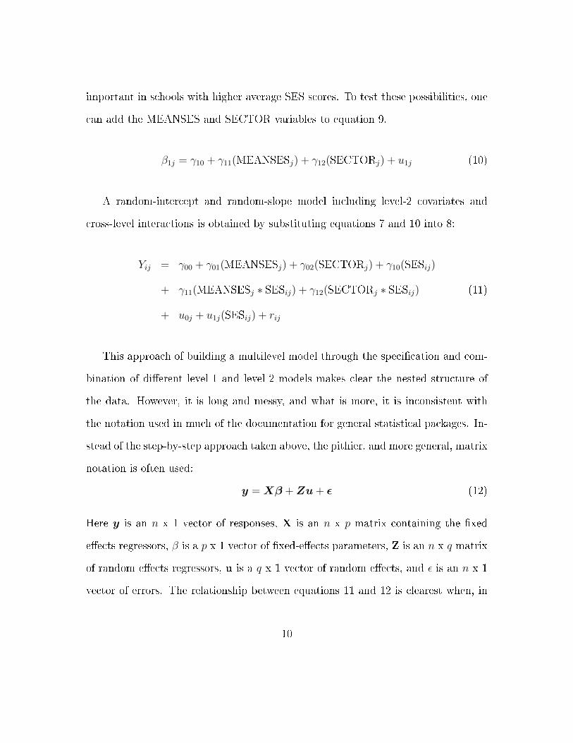
important in schools with higher average SES scores. To test these possibilities, one

can add the MEANSES and SECTOR variables to equation 9.

β1j = γ10 + γ11(MEANSESj) + γ12(SECTORj) + u1j (10)

A random-intercept and random-slope model including level-2 covariates and

cross-level interactions is obtained by substituting equations 7 and 10 into 8:

Yij = γ00 + γ01(MEANSESj) + γ02(SECTORj) + γ10(SESij)

+ γ11(MEANSESj ∗ SESij) + γ12(SECTORj ∗ SESij) (11)

+ u0j + u1j(SESij) + rij

This approach of building a multilevel model through the speci�cation and com-

bination of di�erent level-1 and level-2 models makes clear the nested structure of

the data. However, it is long and messy, and what is more, it is inconsistent with

the notation used in much of the documentation for general statistical packages. In-

stead of the step-by-step approach taken above, the pithier, and more general, matrix

notation is often used:

y =Xβ +Zu+ ε (12)

Here y is an n x 1 vector of responses, X is an n x p matrix containing the �xed

e�ects regressors, β is a p x 1 vector of �xed-e�ects parameters, Z is an n x q matrix

of random e�ects regressors, u is a q x 1 vector of random e�ects, and ε is an n x 1

vector of errors. The relationship between equations 11 and 12 is clearest when, in

10

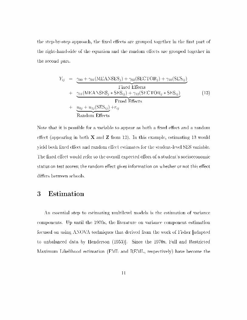
the step-by-step approach, the �xed e�ects are grouped together in the �rst part of

the right-hand-side of the equation and the random e�ects are grouped together in

the second part.

Yij = γ00 + γ01(MEANSESj) + γ02(SECTORj) + γ10(SESij)︸︷︷︸Fixed E�ects

+ γ11(MEANSESj ∗ SESij) + γ12(SECTORj ∗ SESij)︸︷︷︸Fixed E�ects

(13)

+ u0j + u1j(SESij)︸︷︷︸Random E�ects

+rij

Note that it is possible for a variable to appear as both a �xed e�ect and a random

e�ect (appearing in both X and Z from 12). In this example, estimating 13 would

yield both �xed e�ect and random e�ect estimates for the student-level SES variable.

The �xed e�ect would refer to the overall expected e�ect of a student's socioeconomic

status on test scores; the random e�ect gives information on whether or not this e�ect

di�ers between schools.

3 Estimation

An essential step to estimating multilevel models is the estimation of variance

components. Up until the 1970s, the literature on variance component estimation

focused on using ANOVA techniques that derived from the work of Fisher [adapted

to unbalanced data by Henderson (1953)]. Since the 1970s, Full and Restricted

Maximum Likelihood estimation (FML and REML, respectively) have become the

11

preferred methods. ML approaches have several advantages, including the ability to

handle unbalanced data without some of the pathologies of ANOVA methods (i.e.

lack of uniqueness, negative variance estimates). Both FML and REML produce

identical �xed e�ects estimates. The latter, however, takes into account the degrees

of freedom from the �xed e�ects and thus produces variance components estimates

that are less biased. One downside to REML is that the likelihood ratio test cannot

be used to compare two models with di�erent �xed e�ects speci�cations. In small

samples with balanced data, REML is generally preferable to ML because it is unbi-

ased. In large samples, however, di�erences between estimates are neglible (Snijders

and Bosker 1999). Thus, in most applications, �the question of which method to use

remains a matter of personal taste� (StataCorp 2005, pg. 188).

The remainder of this document provides syntax for estimating multilevel models

using SPSS, Stata, SAS, and R. The data analyzed will be the High School and

Beyond (HSB) dataset that accompanies the HLM package (Raudenbush et al. 2005).

Each section will show how to estimate the empty model, a random intercept model,

and a random slope model from the student performance example outlined above.

The dependent variable is scores on a math achievement scale. Note that whereas

HLM requires two separate data �les (one corresponding to each level), SPSS, Stata,

SAS, and R rely on only a single �le. The level-2 observations are common to each

case within the same macro-unit, so that if there are 50 students in one school the

corresponding school-level score appears 50 times.. Each program also requires an id

variable identifying the group membership of each individual. The results presented

below are based on REML estimation, the default in each package.

12

4 SPSS

This section closely follows Peugh and Enders (2005). It demonstrates how to

group-mean center level-1 covariates and estimate multilevel models using SPSS syn-

tax. Note that it is also possible to use the Mixed Models option under the

Analyze pull-down menu (see Norusis 2005, pgs. 197-246). However, length consid-

erations limit the examples here to syntax. The SPSS syntax editor can be accessed

by going to File → New → Syntax.

In the HSB data �le, the student-level SES variable is in its original metric

(a standardized scale with a mean of zero). Oftentimes researchers dealing with

hierarchically structured data wish to center a level-1 variable around the mean

of all cases within the same level-2 group in order to facilitate interpretation of

the intercept. To group-mean center a variable in SPSS, �rst use the AGGREGATE

command to estimate mean SES scores by school. In this example, the syntax would

be:

AGGREGATE OUTFILE=sesmeans.sav

/BREAK=id

/meanses=MEAN(ses) .

The OUTFILE statement speci�es that the means are written out to the �le ses-

means.sav in the working directory. The BREAK subcommand speci�es the groups

within which to estimate means. The �nal line names the variable containing the

school means meanses.

Next, the group means are sorted and merged with the original data using the

SORT CASES and MATCHFILES commands. The centered variables are then created

13

using the COMPUTE command.3 The syntax for these steps would be:

SORT CASES BY id .

MATCH FILES

/TABLE=sesmeans.sav

/FILE=*

/BY id .

COMPUTE centses = ses - meanses .

EXECUTE .

The subcommands for MATCH FILES ask SPSS to take the data �le saved using

the AGGREGATE command and merge it with the working data (denoted by *). The

matching variable is the school ID.

With the data prepared, the next step is to estimate the models of interest. The

following syntax corresponds to the empty model (5):

MIXED mathach

/PRINT = SOLUTION TESTCOV

/FIXED = INTERCEPT

/RANDOM = INTERCEPT | SUBJECT(id) .

The command for estimating multilevel models is MIXED, followed immediately

by the dependent variable. PRINT = SOLUTION requests that SPSS report the �xed

e�ects estimates and standard errors. FIXED and RANDOM specify which variables to

treat as �xed and random e�ects, respectively. The SUBJECT option following the

vertical line | identi�es the grouping variable, in this case school ID.

The �xed and random e�ect estimates for this and subsequent models are dis-

played in Table 1. The intercept in the empty model is equal to the overall average

math achievement score, which for this sample is 12.637. The variance component

3To grand mean center a variable in SPSS requires only a single line of syntax. For example,COMPUTE newvar = oldvar - mean(oldvar).

14

corresponding to the random intercept is 8.614; for the level-1 error it is 39.1483. In

this example, the value of the Wald-Z statistic is 6.254, which is signi�cant (p<.001).

Note, however, that these tests should not be taken as conclusive. Singer (1998, pg.

351) writes,

�the validity of these tests has been called into question both because they

rely on large sample approximations (not useful with the small sample

sizes often analyzed using multilevel models) and because variance com-

ponents are known to have skewed (and bounded) sampling distributions

that render normal approximations such as these questionable.�

A more thorough test would thus estimate a second model constraining the variance

component to equal zero and compare the two models using a likelihood ratio test.

The two variance components can be used to partition the variance across levels

according to equation 6 above. The intraclass correlation coe�cient for this example

is equal to 8.6148.614+39.1483

= .1804, meaning that roughly 18% of the variance is at-

tributable to school traits. Because the intraclass correlation coe�cient shows a fair

amount of variation across schools, model 2 adds two school-level variables. These

variables are sector, de�ning whether a school is private or public, and meanses,

which is the average student socioeconomic status in the school. The SPSS syntax

to estimate this model is:

MIXED mathach WITH meanses sector


/FIXED = INTERCEPT meanses sector

/RANDOM = INTERCEPT | SUBJECT(id) .

The results, displayed in the second column of Table 1, show that meanses and

15

sector signi�cantly a�ect a school's average math achievement score. The inter-

cept, representing the expected math achievement score for a student in a public

school with average SES, is equal to 12.1283. A one unit increase in average SES

raises the expected school mean by 5.5334. Private schools have expected math

achievement scores 1.2254 units higher than public schools. The variance compo-

nent corresponding to the random intercept has decreased to 2.3140, demonstrating

that the inclusion of the two school-level variables has explained much of the level-2

variation. However, the estimate is still more than twice the size of its standard

error, suggesting that there remains a signi�cant amount of unexplained school-level

variance (though the same caution about over-interpreting this test still applies).

A �nal model introduces a student-level covariate, the group-mean centered SES

variable (centses). Because it is possible that the e�ect of socioeconomic status

may vary across schools, SES is treated as a random e�ect. In addition, sector and

meanses are included to model the slope on the student-level SES variable. Modeling

the slope of a random e�ect is the same as specifying a cross-level interaction, which

can be speci�ed in the FIXED subcommand as in the following syntax:

MIXED mathach WITH meanses sector centses


/FIXED = INTERCEPT meanses sector centses meanses*centses sector*centses

/RANDOM = INTERCEPT centses | SUBJECT(id) COVTYPE(UN) .

One important change over the previous models is the addition of the COV(UN)

option, which speci�es a structure for the level-2 covariance matrix. Only a single

school-level variance component was estimated in the previous two models, thus it

was unnecessary to deal with covariances. When there is more than one level-2

16

variance component, SPSS will assume a particular covariance structure. In many

cross-sectional applications of multilevel models, the researcher does not wish to put

any constraints on this covariance matrix. Thus the UN in the COV option speci�es

an unstructured matrix. In other contexts, the researcher may wish to specify a

�rst-order autoregressive (AR1), compound symmetry (CS), identity (ID), or other

structure. These alternatives are more restrictive but may sometimes be appropriate.

The results from this �nal model appear in the last column of Table 1. The

�xed e�ects are all signi�cant. Given the inclusion of the group-mean centered

SES variable, the intercept is interpreted as the expected math achievement in a

public school with average SES levels for a student at his or her school's average

SES. In this model, the expected outcome is 12.1279. Because there are interactions

in the model, the marginal �xed e�ects of each variable will depend on the value

of the other variable(s) involved in the interaction. The marginal e�ect of a one-

unit change in a student's SES score on math achievement depends on whether a

school is public or private as well as on the school's average SES score. For a public

school (where sector=0), the marginal e�ect of a one-unit change in the group-mean

centered student SES variable is equal to ∂Y∂CENTSES

= γ10 + γ11(MEANSES) =

2.945041 + 1.039232(MEANSES). For a private school (where sector=1), the

marginal e�ect of a one-unit change in student SES is equal to ∂Y∂CENTSES

= γ10 +

γ11(MEANSES)+γ12 = 2.945041+1.039232(MEANSES)−1.642674. When cross-

level interactions are present, graphical means may be appropriate for exploring the

contingent nature of marginal e�ects in greater detail (Raudenbush & Bryk 2002;

Brambor, Clark, and Golder 2006). Here the simplest interpretation is that the e�ect

17

of student-level SES is signi�cantly higher in wealthier schools and signi�cantly lower

in private schools.

The variance component for the random intercept continues to be signi�cant,

suggesting that there remains some variation in average school performance not ac-

counted for by the variables in the model. The variance component for the random

slope, however, is not signi�cant. Thus the researcher may be justi�ed in estimating

an alternative model that constrains this variance component to equal zero.

Table 1: Results from SPSS

Fixed E�ects Model 1 Model 2 Model 3

Intercept γ00 12.636974∗ 12.128236∗ 12.127931∗

(0.244394) (0.199193) (0.199290)MEANSES γ01 5.332838∗ 5.3329∗

(0.368623) (0.369164)SECTOR γ02 1.225400∗ 1.226579∗

(0.3058) (0.306269)CENTSES γ10 2.945041∗

(0.155599)MEANSES*CENTSES γ11 1.039232∗

(0.298894)SECTOR*CENTSES γ12 −1.642674∗

(0.239778)

Random E�ects Model 1 Model 2 Model 3

Intercept τ00 8.614025∗ 2.313989∗ 2.379579∗

(1.078804) (0.370011) (0.371456)CENTSES τ11 0.101216

(0.213792)Residual σ2 39.148322∗ 39.161358∗ 36.721155∗

(0.660645) (0.660933) (0.626134)

Model Fit Statistics Model 1 Model 2 Model 3

Deviance 47116.8 46946.5 46714.24AIC 47122.79 46956.5 46726.23BIC 47143.43 46990.9 46767.51

18

5 Stata

This section discusses how to center variables and estimate multilevel models us-

ing Stata. A fuller treatment is available in Rabe-Hesketh and Skrondal (2005) and

in the Stata documentation. Since release 9, Stata includes the command .xtmixed

to estimate multilevel models. The .xt pre�x signi�es that the command belongs

to the larger class of commands used to estimate models for longitudinal data. This

re�ects the fact that panel data can be thought of as multilevel data in which obser-

vations at multiple time points are nested within an individual. However, the com-

mand is appropriate for mixed model estimation in general, including cross-sectional

applications.

In the HSB data �le, the student-level SES variable is in its original metric

(a standardized scale with a mean of zero). Oftentimes researchers dealing with

hierarchically structured data wish to center a level-1 variable around the mean of

all cases within the same level-2 group. Group-mean centering can be accomplished

by using the .egen and .gen commands in Stata.

.egen sesmeans = mean(ses), by(id)

.gen centses = ses - sesmeans

Here .egen generates a new variable sesmeans , which is the mean of ses for

all cases within the same level-2 group. The subsequent line of code generates a new

variable centses, which is centered around the mean of all cases within each level-2

group.

The syntax for estimating multilevel models in Stata begins with the .xtmixed

command followed by the dependent variable and a list of independent variables.

19

The last independent variable is followed by double vertical lines ||, after which the

grouping variable and random e�ects are speci�ed. .xtmixed will automatically

specify the intercept to be random. A list of variables whose slopes are to be treated

as random follows the colon. Note that, by default, Stata reports variance compo-

nents as standard deviations (equal to the square root of the variance components).

To get Stata to report variances instead, add the var option. The syntax for the

empty model is the following:

.xtmixed mathach || id: , var

The results are displayed in Table 2. The average test score across schools,

re�ected in the intercept term, is 12.63697. The variance component corresponding

to the random intercept is 8.61403. Because this estimate is substantially larger than

its standard error, there appears to be signi�cant variation in school means.

The two variance components can be used to partition the variance across levels.

The intraclass correlation coe�cient is equal to 8.6140339.14832+8.61403

= 18.04, meaning that

roughly 18% of the variance is attributable to the school-level.

In order to explain some of the school-level variance in math achievement scores

it is possible to incorporate school-level predictors into the model. For example,

the socioeconomic status of the typical student, or the school's status as public or

private, may in�uence test performance. The Stata syntax for adding these variables

to the model is:

.xtmixed mathach meanses sector || id: , var

The intercept, which now corresponds to the expected math achievement score

in a public school with average SES scores, is 12.12824. Moving to a private school

20

bumps the expected score by 1.2254 points. In addition, a one-unit increase in the

average SES score is associated with an expected increased in math achievement of

5.3328. These estimates are all signi�cant.

The variance component corresponding to the random intercept has decreased to

2.313986, re�ecting the fact that the inclusion of the level-2 variables has accounted

for some of the variance in the dependent variable. Nonetheless, the estimate is still

more than twice the size of its standard error, suggesting that there remains variance

unaccounted for.

A �nal model introduces the student socioeconomic status variable. Because it

is possible that the e�ect of individual SES status varies across schools, this slope is

treated as random. In addition, a school's average SES score and its sector (public

or private) may interact with student-level SES, accounting for some of the variance

in the slope. In order to include these cross-level interactions in the model, however,

it is necessary to �rst explicitly create the interaction variables in Stata:

.gen ses_mses=meanses*centses

.gen ses_sect=sector*centses

When estimating more than one random e�ect, the researcher must also be con-

cerned with the covariances among the level-2 variance components. As with SPSS,

in Stata it is necessary to add an option specifying that the covariance matrix for

the random e�ects is unstructured (the default is to assume all covariances are zero).

The syntax for estimating the random-slope model is thus:

.xtmixed mathach meanses sector centses ses_mses ses_sect || id: centses,

var cov(un)

The results are displayed in the �nal column of Table 2. The intercept is 12.12793,

21

which here is the expected math achievement score in a public school with average

SES scores for a student at his or her school's average SES level. Because there are

interactions in the model, the marginal �xed e�ects of each variable now depend on

the value of the other variable(s) involved in the interaction. The marginal e�ect of

a one-unit change in student's SES on math achievement will depend on whether a

school is public or private as well as on the average SES score for the school. For

a public school (where sector=0), the marginal e�ect of a one-unit change in the

group-mean centered SES variable is equal to ∂Y∂CENTSES

= γ10+γ11(MEANSES) =

2.94504 + 1.039237(MEANSES). For a private school (where sector=1), the

marginal e�ect of a one-unit change in student SES is equal to ∂Y∂CENTSES

= γ10 +

γ11(MEANSES)+γ12 = 2.94504+1.039237(MEANSES)−1.642675. When cross-

level interactions are present, graphical means may be appropriate for exploring the

contingent nature of marginal e�ects in greater detail. Here the simplest interpreta-

tion of the interaction coe�cients is that the e�ect of student-level SES is signi�cantly

higher in wealthier schools and signi�cantly lower in private schools.

The variance component for the random intercept is 2.379597, which is still large

relative to its standard error of 0.3714584. Thus there remains some school-level

variance unaccounted for in the model. The variance component corresponding to

the slope, however, is quite small relative to its standard error. This suggests that

the researcher may be justi�ed in constraining the e�ect to be �xed.

By default, Stata does not report model �t statistics such as the AIC or BIC.

These can be requested, however, by using the postestimation command .estat ic.

This displays the log-likelihood, which can be converted to Deviance according to the

22

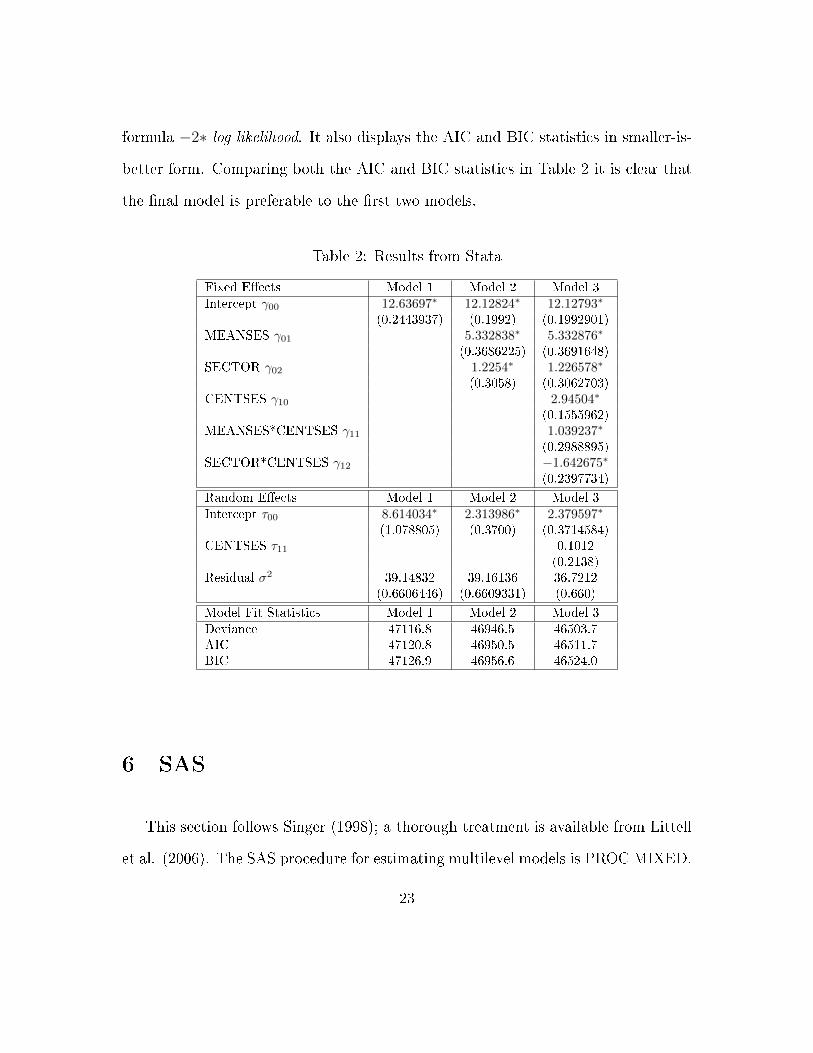
formula −2∗ log likelihood. It also displays the AIC and BIC statistics in smaller-is-

better form. Comparing both the AIC and BIC statistics in Table 2 it is clear that

the �nal model is preferable to the �rst two models.

Table 2: Results from Stata


Intercept γ00 12.63697∗ 12.12824∗ 12.12793∗

(0.2443937) (0.1992) (0.1992901)MEANSES γ01 5.332838∗ 5.332876∗

(0.3686225) (0.3691648)SECTOR γ02 1.2254∗ 1.226578∗

(0.3058) (0.3062703)CENTSES γ10 2.94504∗


(0.2988895)SECTOR*CENTSES γ12 −1.642675∗

(0.2397734)


Intercept τ00 8.614034∗ 2.313986∗ 2.379597∗

(1.078805) (0.3700) (0.3714584)CENTSES τ11 0.1012

(0.2138)Residual σ2 39.14832 39.16136 36.7212

(0.6606446) (0.6609331) (0.660)


Deviance 47116.8 46946.5 46503.7AIC 47120.8 46950.5 46511.7BIC 47126.9 46956.6 46524.0

6 SAS

This section follows Singer (1998); a thorough treatment is available from Littell

et al. (2006). The SAS procedure for estimating multilevel models is PROC MIXED.

23

In the HSB data �le the student-level SES variable is in its original metric (a

standardized scale with a mean of zero). Oftentimes, the researcher will prefer to

center a variable around the mean of all observations within the same group. Group-

mean centering in SAS is accomplished using the SQL procedure. The following

commands create a new data �le, HSB2, in the Work library that includes two

additional variables: the group means for the SES variable (saved as the variable

sesmeans) and the group-mean centered SES variable cses.4

PROC SQL;

CREATE TABLE hsb2 AS

SELECT *, mean(ses) as meanses,

ses-mean(ses) AS cses

FROM hsb

GROUP BY id;

QUIT;

The syntax for estimating the empty model is the following:

PROC MIXED COVTEST DATA=hsb2;

CLASS id;

MODEL mathach = /SOLUTION;

RANDOM intercept/SUBJECT=id

RUN;

The COVTEST option requests hypothesis tests for the random e�ects. The CLASS

statement identi�es id as a categorical variable. The MODEL statement de�nes the

model, which in this case does not include any predictor variables, and the SOLUTION

option asks SAS to print the �xed e�ects estimates in the output. The next state-

ment, RANDOM, identi�es the elements of the model to be speci�ed as random e�ects.

4Grand-mean centering also uses PROC SQL. Excluding the GROUP BY statement causes themean(ses) function to estimate the grand mean for the ses variable. The ses-mean(ses) state-ment then creates the grand-mean centered variable.

24

The SUBJECT=id option identi�es id to be the grouping variable.

The results are displayed in Table 3. The average math achievement score across

all schools is 12.6370. The variance component corresponding to the random inter-

cept is 8.6097, which has a corresponding standard error of 1.0778. Because this

estimate is more than twice the size of its standard error, there is evidence of signif-

icant variation in average test scores across schools (though see the SPSS section for

a caution on over-interpreting this test).

It is possible to partition the variance in the dependent variable across levels

according to the ratio of the school-level variance component to the total variance.

In this example, the ratio is 8.60978.6097+39.1487

= .1802761, meaning that roughly 18% of

the variance is attributable to school characteristics.

In order to explain some of the school-level variation in math achievement scores

it is possible to incorporate school-level predictors into the model. For example,

the average socioeconomic status of a school's students may a�ect performance. In

addition, whether a school is public or private may also make a di�erence. The SAS

program for a model with two school level predictors is the following:


CLASS id;

MODEL mathach = meanses sector /SOLUTION;

RANDOM intercept/SUBJECT=id;

RUN;

The MODEL statement now includes the two school-level predictors following the

equals sign. Nothing else is changed from the previous program.

The results are displayed in the second column of Table 3. The intercept is

12.1282, which now corresponds to the expected math achievement score for a student

25

in a public school at that school's average SES level. A one-unit increase in the

school's average SES score is associated with a 5.3328-unit increase in expected

math achievement, and moving from a public to a private school is associated with

an expected improvement of 1.2254. These estimates are all signi�cant.

The variance component corresponding to the random intercept has now dropped

to 2.3139, demonstrating that the inclusion of the average SES and school sector

variables explains a good deal of the school-level variance. Still, the estimate remains

more than twice the size of its standard error of 0.3700, suggesting that some of the

school-level variance remains unexplained.

A �nal model adds a student-level covariate, the group-mean centered SES vari-

able. Because it is possible that the e�ect of a student's SES may vary across schools,

the �nal model treats the slope as random. Additionally, because the slope may vary

according to school-level characteristics such as average SES and sector (private ver-

sus public), the �nal model also incorporates cross-level interactions.

The syntax for this last model is the following:


CLASS id;

MODEL mathach = meanses sector cses meanses*cses sector*cses/solution;

RANDOM intercept cses / TYPE=UN SUB=id;

RUN;

The MODEL statement adds the cses variable along with the cross-level inter-

actions between cses at the student level and sector and meanses at the school

level. CSES is also added to the RANDOM statement. The TYPE=UN option speci�es

an unstructured covariance matrix for the random e�ects.

The results are displayed in the �nal column of Table 3. The intercept of 12.1279

26

now refers to the expected math achievement score in a public school with average

SES scores for a student at his or her school's average SES level. Because there

are interactions in the model, the marginal �xed e�ects of each variable depend on

the value of the other variable(s) involved in the interaction. The marginal e�ect

of a one-unit change in a student's SES score on math achievement will depend

on whether a school is public or private as well as on the school's average SES

score. For a public school (where sector=0), the marginal e�ect of a one-unit

change in the group-mean centered student SES variable is equal to ∂Y∂CENTSES

=

γ10+γ11(MEANSES) = 2.9450+1.0392(MEANSES). For a private school (where

sector=1), the marginal e�ect of a one-unit change in a student's SES is equal to

∂Y∂CENTSES

= γ10+γ11(MEANSES)+γ12 = 2.9450+1.0392(MEANSES)−1.6427.

When cross-level interactions are present, graphical means may be appropriate for

exploring the contingent nature of marginal e�ects in greater detail. Here the simplest

interpretation of the interaction coe�cients is that the e�ect of student-level SES is

signi�cantly higher in wealthier schools and signi�cantly lower in private schools.

The variance component corresponding to the random intercept is 2.3794, which

remains much larger than its standard error of .3714. Thus there is most likely addi-

tional school-level variation unaccounted for in the model. The variance component

for the random slope is smaller than its standard error, however, suggesting that the

model picks up most of the variance in this slope that exists across schools.

27

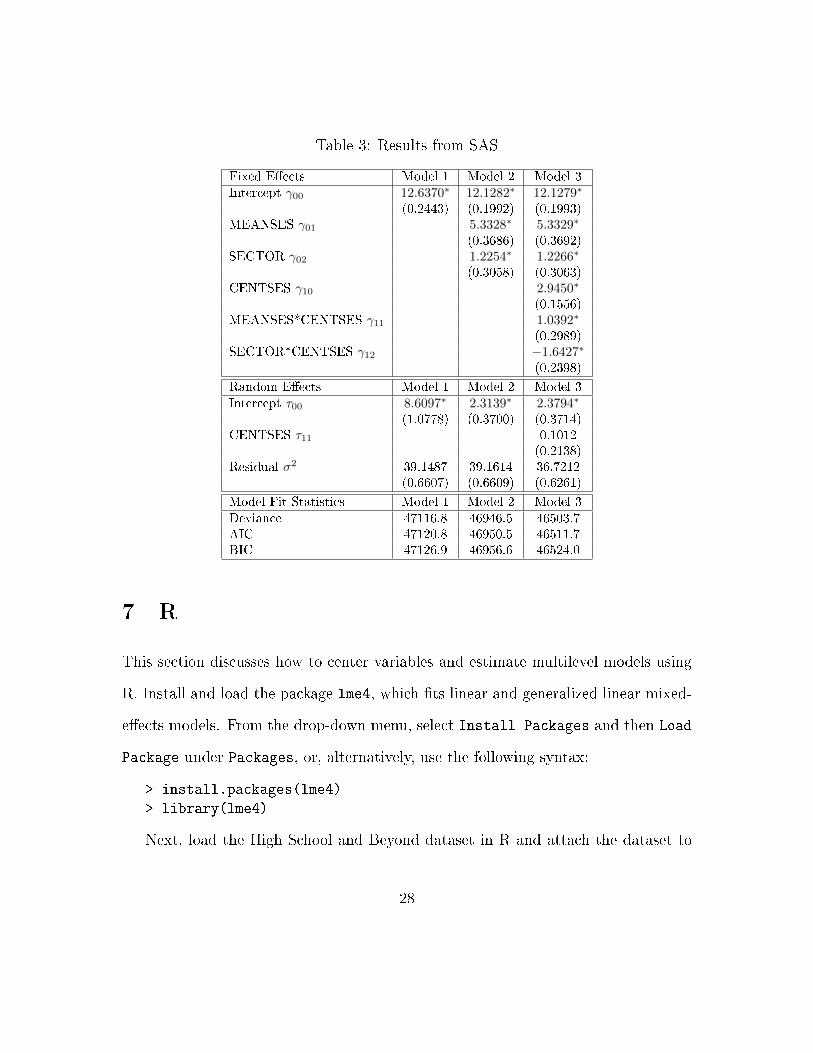
Table 3: Results from SAS


Intercept γ00 12.6370∗ 12.1282∗ 12.1279∗

(0.2443) (0.1992) (0.1993)MEANSES γ01 5.3328∗ 5.3329∗

(0.3686) (0.3692)SECTOR γ02 1.2254∗ 1.2266∗

(0.3058) (0.3063)CENTSES γ10 2.9450∗


(0.2989)SECTOR*CENTSES γ12 −1.6427∗

(0.2398)


Intercept τ00 8.6097∗ 2.3139∗ 2.3794∗

(1.0778) (0.3700) (0.3714)CENTSES τ11 0.1012

(0.2138)Residual σ2 39.1487 39.1614 36.7212

(0.6607) (0.6609) (0.6261)


Deviance 47116.8 46946.5 46503.7AIC 47120.8 46950.5 46511.7BIC 47126.9 46956.6 46524.0

7 R

This section discusses how to center variables and estimate multilevel models using

R. Install and load the package lme4, which �ts linear and generalized linear mixed-

e�ects models. From the drop-down menu, select Install Packages and then Load

Package under Packages, or, alternatively, use the following syntax:

> install.packages(lme4)

> library(lme4)

Next, load the High School and Beyond dataset in R and attach the dataset to

28

the R search path:

> HSBdata <- read.table("C:/user/temp/hsbALL.txt", header=T, sep=",")

> attach(HSBdata)

To center a level-1 variable around the mean of all cases within the same level-2

group, use the ave() function, which estimates group averages. The new variable

meanses is the average of ses for each high school group id. The new variable

centses is centered around the mean of all cases within each level-2 group by sub-

tracting meanses from ses. The text HSBdata$, which is attached to the new vari-

able name, indicates that the variables will be created within the existing dataset

HSBdata. Remember to attach the dataset to the R search path after making any

changes to the variables.

> HSBdata$meanses <- ave(ses, list(id))

> HSBdata$centses <- ses - meanses

> attach(HSBdata)

Within the lme4 package, the lme() function estimates linear mixed e�ects mod-

els. To use lme(), specify the dependent variable, the �xed components after the

tilde sign and the random components in parentheses. Indicate which dataset R

should use. To �t the empty model described above (5), use the following sintax:

> results1 <- lmer(mathach ∼ 1 + (1 | id), data = HSBdata)

> summary(results1)

R saves the results of the model in an object called results1, which is stored in

memory and may be retrieved with the function summary(). The function lmer()

estimates a model, in which mathach is the dependent variable. The intercept,

denoted by 1 immediately following the tilde sign, is the intercept for the �xed

e�ects. Within the parentheses, 1 denotes the random e�ects intercept, and the

29

variable id is speci�ed as the level-2 grouping variable. R uses the HSBdata for this

analysis.

The results are displayed in Table 4. The average test score across schools,

re�ected in the �xed e�ects intercept term, is 12.6370. The variance component

corresponding to the random intercept is 8.614. The two variance components can

be used to partition the variance across levels. The intraclass correlation coe�cient is

equal to 8.61439.148+8.614

= 18.04, meaning that roughly 18% of the variance is attributable

to the school-level.

To explain some of the school-level variance in student math achievement scores,

incorporate school-level predictors in the empty the model. The socioeconomic status

of the typical student and the school's status as public or private may in�uence test

performance. The following R syntax indicates how to incorporate these two variables

as �xed e�ects:

> results2 <- lmer(mathach ∼ 1 + sesmeans + sector + (1 | id), data

= HSBdata)

> summary(results2)

The intercept, which now corresponds to the expected math achievement score

in a public school with average SES scores, is 12.1282. Moving to a private school

bumps the expected score by 1.2254 points. In addition, a one-unit increase in the

average SES score is associated with an expected increased in math achievement of

5.3328. These estimates are all signi�cant.

The variance component corresponding to the random intercept has decreased to

2.3140, indicating that the inclusion of the level-2 variables has accounted for some

of the unexplained variance in the math achievement. Nonetheless, the estimate is

30

still more than twice the size of its standard error, suggesting that there remains

unexplained variance.

The �nal model introduces the student socioeconomic status (SES) variable and

cross-level interaction terms. The centered SES slope is treated as random because

individual SES status may vary across schools. In addition, a school's average SES

score and its sector (public or private) may interact with student-level SES, thus

accounting for some of the variance in the math achievement slope. To include cross-

level interaction terms in your model, place an asterisk between the two variables

composing the interaction.

> results3 <- lmer(mathach ∼ sesmeans + sector + centses + sesmeans*centses

+ sector*centses + (1 + centses|id), data = HSBdata)

> summary(results3)

The results are displayed in the �nal column of Table 4. Because there are

interactions in the model, the marginal �xed e�ects of each variable now depend

on the value of the other variable(s) involved in the interaction. The marginal

e�ect of a one-unit change in student's SES on math achievement will depend

on whether a school is public or private as well as on the average SES score for

the school. For a public school (where sector=0), the marginal e�ect of a one-

unit change in the group-mean centered SES variable is equal to ∂Y∂CENTSES

=

γ10+γ11(MEANSES) = 2.9450+1.0392(MEANSES). For a private school (where

sector=1), the marginal e�ect of a one-unit change in student SES is equal to

∂Y∂CENTSES

= γ10+γ11(MEANSES)+γ12 = 2.9450+1.0392(MEANSES)−1.6427.

When cross-level interactions are present, graphical means may be appropriate for ex-

ploring the contingent nature of marginal e�ects in greater detail. Here the simplest

31

interpretation of the interaction coe�cients is that the e�ect of student-level SES is

signi�cantly higher in wealthier schools and signi�cantly lower in private schools.

The variance component for the random intercept is 2.37956, which is still large

relative to its standard deviation of 1.54258. Thus some school-level variance remains

unexmplained in the �nal model. The variance component corresponding to the

slope, however, is quite small relative to its standard deviation. This suggests that

the researcher may be justi�ed in constraining the e�ect to be �xed.

R displays the deviance and AIC and BIC. Comparing both the AIC and BIC

statistics in Table 4 it is clear that the �nal model is preferable to the �rst two

models.

32

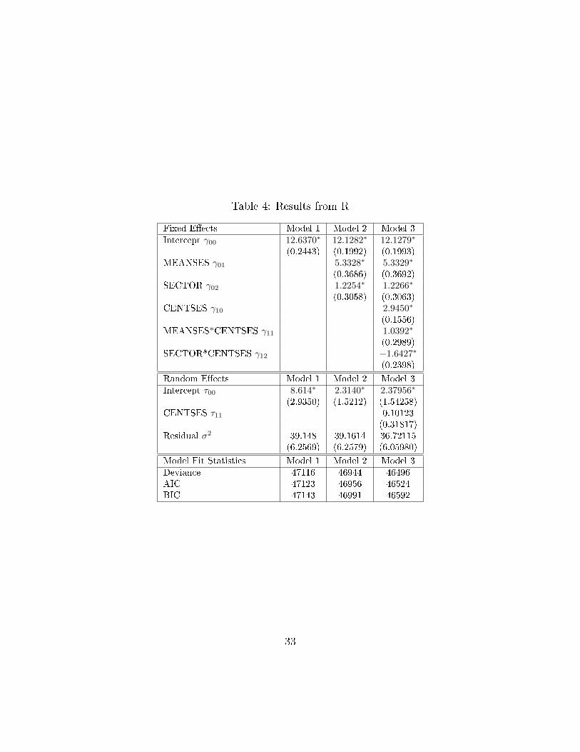
Table 4: Results from R


Intercept γ00 12.6370∗ 12.1282∗ 12.1279∗

(0.2443) (0.1992) (0.1993)MEANSES γ01 5.3328∗ 5.3329∗

(0.3686) (0.3692)SECTOR γ02 1.2254∗ 1.2266∗

(0.3058) (0.3063)CENTSES γ10 2.9450∗


(0.2989)SECTOR*CENTSES γ12 −1.6427∗

(0.2398)


Intercept τ00 8.614∗ 2.3140∗ 2.37956∗

(2.9350) (1.5212) (1.54258)CENTSES τ11 0.10123

(0.31817)Residual σ2 39.148 39.1614 36.72115

(6.2569) (6.2579) (6.05980)


Deviance 47116 46944 46496AIC 47123 46956 46524BIC 47143 46991 46592

33

References

[1] Brambor, T., Clark, W. R., & Golder, M. (2006). Understanding interaction models:

Improving emprical analysis. Political Analysis, 14, 63-82.

[2] Ferron, J. (1997). Moving between hierarchical modeling notations. Journal of Educa-

tional and Behavioral Statistics, 22, 119-12.

[3] Hayes, W. L. (1973). Statistics for the Social Sciences. New York: Holt, Rinehart, &

Winston

[4] Henderson, C. R. (1953). Estimation of variance and covariance components. Biomet-

rics, 9, 226-252.

[5] Hox, J. J. (1994). Multilevel analysis methods. Sociological Methods & Research, 22,

283-299.

[6] Littell, R. C., Milliken, G. A., Stroup, W. A., Wol�nger, R. D., & Schabenberger, O.

(2006). SAS for Mixed Models, Second Edition. Cary, NC: SAS Institute.

[7] Maxwell, S. E. & Delaney, H. D. (2004). Designing Experiments and Analyzing Data:

A Model Comparison Perspective, Second Edition. Mahwah, NJ: Lawrence Erlbaum

Associates, Inc.

[8] Norusis, M. J. (2005). SPSS 14.0 Advanced Statistical Procedures Companion. Upper

Saddle, NJ: Prentice Hall.

[9] Peugh, J. L. & Enders, C. K. (2005). Using the SPSS mixed procedure to �t cross-

sectional and longitudinal multilevel models. Educational and Psychological Measure-

ment , 65, 714-741.

34

[10] Raudenbush, S.W. & Bryk, A. S. (2002). Hierarchical Linear Models: Applications

and Data Analysis Methods, Second Edition. Newbury Park, CA: Sage.

[11] Raudenbush, S., Bryk, A., Cheong, Y. F., & Congdon, R. (2005). HLM 6: Hierarchical

Linear and Nonlinear Modeling. Lincolnwood, IL: Scienti�c Software International.

[12] Rabe-Hesketh, S. & Skrondal A. (2005). Multilevel and Longitudinal Modeling using

Stata. College Station, TX: StataCorp LP.

[13] Searle, S. R., Casella, G., & McCulloch, C. E. (1992). Variance Components. New

York: Wiley.

[14] Singer, J. D. (1998). Using SAS PROC MIXED to �t multilevel models, hierarchical

models, and individual growth models. Journal of Educational and Behavioral Statis-

tics, 24, 323-355.

[15] Snijders, T. A. B., & Bosker, R. J. (1999). Multilevel Analysis: An Introduction to

Basic and Advanced Multilevel Modeling . Thousand Oaks, CA: Sage.

[16] StataCorp. (2005). Stata Longitudinal/Panel Data Reference Manual, Release 9 . Col-

lege Station, TX: StataCorp LP.

35

Documents

Estimating Multilevel Models using SPSS, Stata, SAS, and R