Embed Size (px)
Citation preview

Estimating extremal dependence using
B-splines
Christian Genest & Johanna G. NeslehovaMcGill University, Montreal, Canada
June 16, WU Wien
Joint work with A. Bucher and D. Sznajder
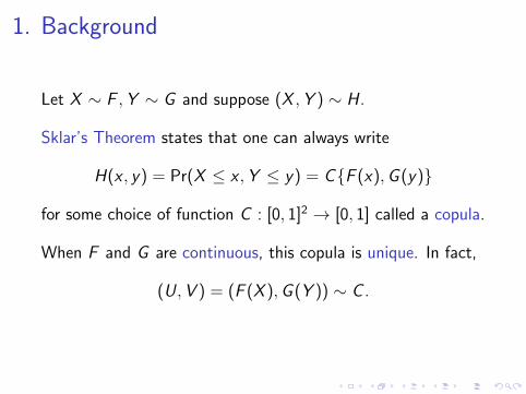
Outline
1. Background
2. Extreme-value copulas
3. A new diagnostic tool: The A-plot
4. An intrinsic estimator based on B-splines
5. Simulation results and data illustration
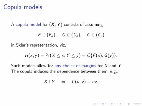
1. Background
Let X ∼ F ,Y ∼ G and suppose (X ,Y ) ∼ H .
Sklar’s Theorem states that one can always write
H(x , y) = Pr(X ≤ x ,Y ≤ y) = C{F (x),G (y)}
for some choice of function C : [0, 1]2 → [0, 1] called a copula.
When F and G are continuous, this copula is unique. In fact,
(U ,V ) = (F (X ),G (Y )) ∼ C .
Copula models
A copula model for (X ,Y ) consists of assuming
F ∈ (Fα), G ∈ (Gβ), C ∈ (Cθ)
in Sklar’s representation, viz.
H(x , y) = Pr(X ≤ x ,Y ≤ y) = C{F (x),G (y)}.
Such models allow for any choice of margins for X and Y .The copula induces the dependence between them, e.g.,
X⊥Y ⇔ C (u, v) ≡ uv .
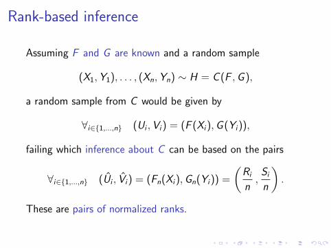
Rank-based inference
Assuming F and G are known and a random sample
(X1,Y1), . . . , (Xn,Yn) ∼ H = C (F ,G ),
a random sample from C would be given by
∀i∈{1,...,n} (Ui ,Vi) = (F (Xi),G (Yi)),
failing which inference about C can be based on the pairs
∀i∈{1,...,n} (Ui , Vi) = (Fn(Xi),Gn(Yi)) =
(Ri
n,Si
n
).
These are pairs of normalized ranks.
Theoretical justification
Consider the empirical distribution function
Cn(u, v) =1
n
n∑i=1
1(Ui ≤ u, Vi ≤ v)
known as the empirical copula.
Suppose C is “sufficiently smooth”; see, e.g.,
I Ruschendorf (1976);
I Fermanian, Radulovic & Wegkamp (2004);
I Segers (2012).
Fundamental result
As n→∞, √n (Cn − C ) CC ,
where
CC (u, v) = α(u, v)− ∂C (u, v)
∂uα(u, 1)− ∂C (u, v)
∂vα(1, v).
and α is a centered Gaussian random field on [0, 1]2 withcovariance function
cov{α(u, v), α(u′, v ′)} = C (u ∧ u′, v ∧ v ′)− C (u, v)C (u′, v ′).
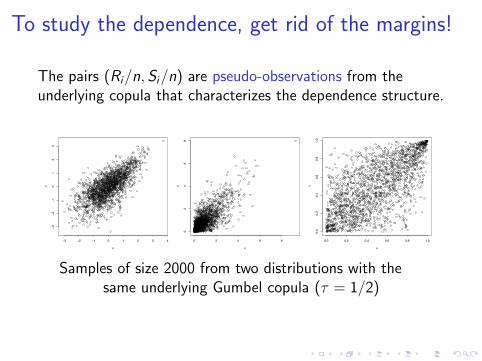
To study the dependence, get rid of the margins!
The pairs (Ri/n, Si/n) are pseudo-observations from theunderlying copula that characterizes the dependence structure.
3 2 1 0 1 2 3 4
32
10
12
3
x
y
0 2 4 6 8
02
46
8
x
y
0.0 0.2 0.4 0.6 0.8 1.0
0.0
0.2
0.4
0.6
0.8
1.0
u
v
Samples of size 2000 from two distributions with thesame underlying Gumbel copula (τ = 1/2)
2. Extreme-value copulas
Extreme-value copulas are the asymptotic dependencestructures of component-wise maxima.
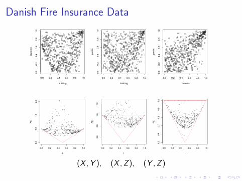
Modeling joint extremes is a key issue in risk management. Aclassical example (McNeil 1997) is
I X : damage to buildings
I Y : loss to contents
I Z : loss of profits
from losses of 1M DKK to the Copenhagen Reinsurancecompany arising from fire claims between 1980 and 1990.
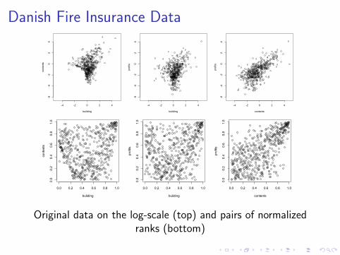
Danish Fire Insurance Data
-4 -2 0 2 4
-6-4
-20
24
building
contents
-4 -2 0 2 4
-6-4
-20
24
building
profits
-4 -2 0 2 4
-6-4
-20
24
contents
profits
0.0 0.2 0.4 0.6 0.8 1.0
0.0
0.2
0.4
0.6
0.8
1.0
buliding
contents
0.0 0.2 0.4 0.6 0.8 1.0
0.0
0.2
0.4
0.6
0.8
1.0
buliding
profits
0.0 0.2 0.4 0.6 0.8 1.0
0.0
0.2
0.4
0.6
0.8
1.0
contents
profits
Original data on the log-scale (top) and pairs of normalizedranks (bottom)
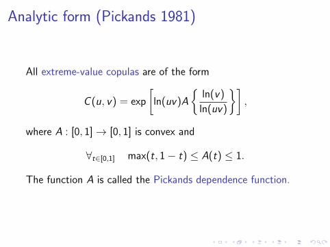
Analytic form (Pickands 1981)
All extreme-value copulas are of the form
C (u, v) = exp
[ln(uv)A
{ln(v)
ln(uv)
}],
where A : [0, 1]→ [0, 1] is convex and
∀t∈[0,1] max(t, 1− t) ≤ A(t) ≤ 1.
The function A is called the Pickands dependence function.
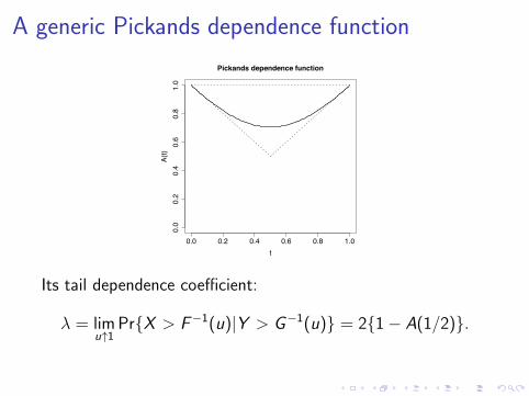
A generic Pickands dependence function
0.0 0.2 0.4 0.6 0.8 1.0
0.0
0.2
0.4
0.6
0.8
1.0
Pickands dependence function
t
A(t)
Its tail dependence coefficient:
λ = limu↑1
Pr{X > F−1(u)|Y > G−1(u)} = 2{1− A(1/2)}.
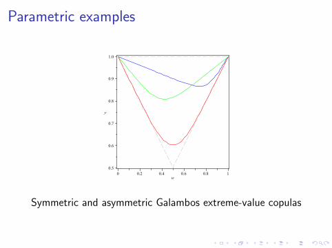
Parametric examples
Symmetric and asymmetric Galambos extreme-value copulas

Focus of today’s talk
Suppose (X1,Y1), . . . , (Xn,Yn) is a random sample from
H(x , y) = C{F (x),G (y)},
where F ,G are continuous and C is a copula.
I How can one decide whether C is extreme-value?
I If an extreme-value copula model is appropriate, how canA be estimated intrinsically?
That is, we want An to be convex and such that
∀t∈[0,1] max(t, 1− t) ≤ An(t) ≤ 1.
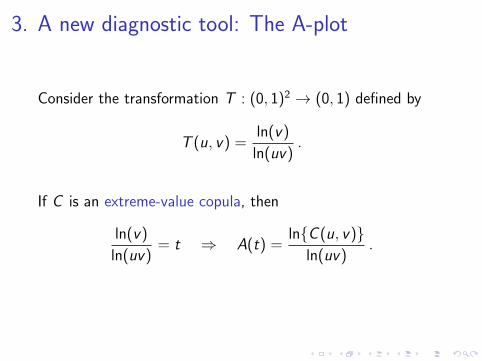
3. A new diagnostic tool: The A-plot
Consider the transformation T : (0, 1)2 → (0, 1) defined by
T (u, v) =ln(v)
ln(uv).
If C is an extreme-value copula, then
ln(v)
ln(uv)= t ⇒ A(t) =
ln{C (u, v)}ln(uv)
.
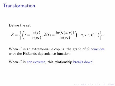
Transformation
Define the set
S =
{(t =
ln(v)
ln(uv),A(t) =
ln{C (u, v)}ln(uv)
): u, v ∈ (0, 1)
}.
When C is an extreme-value copula, the graph of S coincideswith the Pickands dependence function.
When C is not extreme, this relationship breaks down!
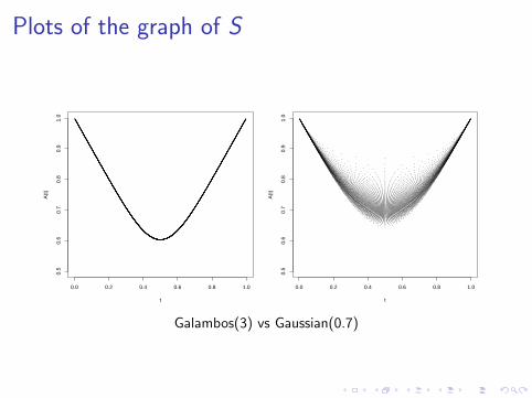
Plots of the graph of S
0.0 0.2 0.4 0.6 0.8 1.0
0.5
0.6
0.7
0.8
0.9
1.0
t
A(t
)
0.0 0.2 0.4 0.6 0.8 1.00.
50.
60.
70.
80.
91.
0
t
A(t
)
Galambos(3) vs Gaussian(0.7)
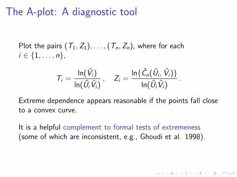
The A-plot: A diagnostic tool
Plot the pairs (T1,Z1), . . . , (Tn,Zn), where for eachi ∈ {1, . . . , n},
Ti =ln(Vi)
ln(Ui Vi), Zi =
ln{Cn(Ui , Vi)}ln(Ui Vi)
.
Extreme dependence appears reasonable if the points fall closeto a convex curve.
It is a helpful complement to formal tests of extremeness(some of which are inconsistent, e.g., Ghoudi et al. 1998).
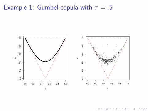
Example 1: Gumbel copula with τ = .5
0.0 0.2 0.4 0.6 0.8 1.0
0.5
0.6
0.7
0.8
0.9
1.0
t
A
0.0 0.2 0.4 0.6 0.8 1.00.5
0.6
0.7
0.8
0.9
1.0
t
A

Example 2: Gaussian copula with τ = .5
0.0 0.2 0.4 0.6 0.8 1.0
0.5
0.6
0.7
0.8
0.9
1.0
t
A
0.0 0.2 0.4 0.6 0.8 1.00.5
0.6
0.7
0.8
0.9
1.0
t
A
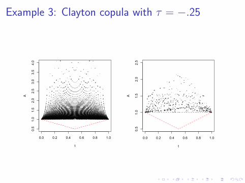
Example 3: Clayton copula with τ = −.25
0.0 0.2 0.4 0.6 0.8 1.0
0.5
1.0
1.5
2.0
2.5
3.0
3.5
4.0
t
A
0.0 0.2 0.4 0.6 0.8 1.00.5
1.0
1.5
2.0
2.5
t
A
Danish Fire Insurance Data
0.0 0.2 0.4 0.6 0.8 1.0
0.0
0.2
0.4
0.6
0.8
1.0
buliding
contents
0.0 0.2 0.4 0.6 0.8 1.0
0.0
0.2
0.4
0.6
0.8
1.0
buliding
profits
0.0 0.2 0.4 0.6 0.8 1.0
0.0
0.2
0.4
0.6
0.8
1.0
contents
profits
0.0 0.2 0.4 0.6 0.8 1.0
0.5
1.0
1.5
2.0
t
A(t)
0.0 0.2 0.4 0.6 0.8 1.0
0.6
0.8
1.0
1.2
t
A(t)
0.0 0.2 0.4 0.6 0.8 1.0
0.5
0.6
0.7
0.8
0.9
1.0
tA(t)
(X ,Y ), (X ,Z ), (Y ,Z )
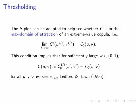
Thresholding
The A-plot can be adapted to help see whether C is in themax-domain of attraction of an extreme-value copula, i.e.,
lim`→∞
C `(u1/`, v 1/`) = C0(u, v).
This condition implies that for sufficiently large w ∈ (0, 1),
C (u, v) ≈ C1/`0 (u`, v `) = C0(u, v)
for all u, v > w ; see, e.g., Ledford & Tawn (1996).

Illustration (Student t2 with ρ = 0.7)
0.0 0.2 0.4 0.6 0.8 1.0
0.5
0.6
0.7
0.8
0.9
1.0
t
A
0.0 0.2 0.4 0.6 0.8 1.0
0.5
0.6
0.7
0.8
0.9
1.0
t
A
0.0 0.2 0.4 0.6 0.8 1.0
0.5
0.6
0.7
0.8
0.9
1.0
t
A
0.0 0.2 0.4 0.6 0.8 1.0
0.5
0.6
0.7
0.8
0.9
1.0
t
A
Threshold w ∈ {0, .25, .5, .75}, n = 1000
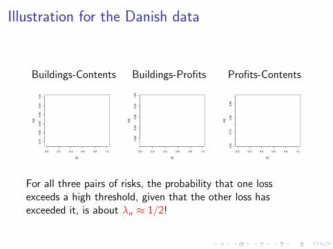
Illustration for the Danish data
Buildings-Contents Buildings-Profits Profits-Contents
0.0 0.2 0.4 0.6 0.8 1.0
0.75
0.80
0.85
0.90
0.95
1.00
t[I]
A[I]
0.0 0.2 0.4 0.6 0.8 1.0
0.80
0.85
0.90
0.95
1.00
t[I]
A[I]
0.0 0.2 0.4 0.6 0.8 1.0
0.65
0.75
0.85
0.95
t[I]
A[I]
For all three pairs of risks, the probability that one lossexceeds a high threshold, given that the other loss hasexceeded it, is about λu ≈ 1/2!
4. An intrinsic estimator based on B-splines
Many estimators of A have been proposed so far; see, e.g.,
I Pickands (1981), Caperaa & Fougeres & Genest (1997),Genest & Segers (2009)
I Deheuvels (1991), Hall & Tajvidi (2000), Jimenez,Villa-Diharce & Flores (2001), Segers (2007)
I Zhang, Wells & Peng (2007), Gudendorf & Segers (2012)
I Bucher, Dette & Volgushev (2011), Berghaus, Bucher &Dette (2012)
I Guillotte & Perron (2008), Guillotte, Perron & Segers(2011), Guillotte & Perron (2012)
I Ucer & Ahmadabadi (Bernstein polynomials, in progress)
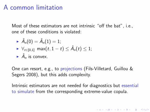
A common limitation
Most of these estimators are not intrinsic “off the bat”, i.e.,one of these conditions is violated:
I An(0) = An(1) = 1;
I ∀t∈[0,1] max(t, 1− t) ≤ An(t) ≤ 1;
I An is convex.
One can resort, e.g., to projections (Fils-Villetard, Guillou &Segers 2008), but this adds complexity.
Intrinsic estimators are not needed for diagnostics but essentialto simulate from the corresponding extreme-value copula.
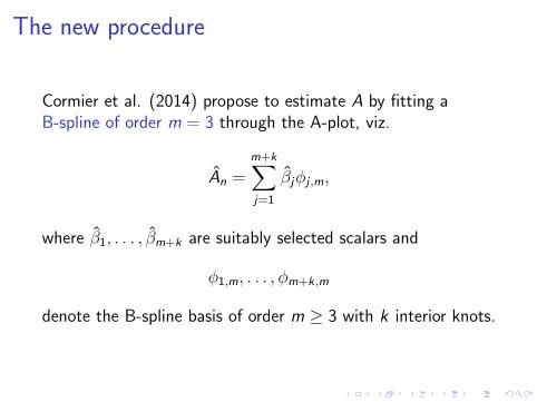
The new procedure
Cormier et al. (2014) propose to estimate A by fitting aB-spline of order m = 3 through the A-plot, viz.
An =m+k∑j=1
βjφj ,m,
where β1, . . . , βm+k are suitably selected scalars and
φ1,m, . . . , φm+k,m
denote the B-spline basis of order m ≥ 3 with k interior knots.
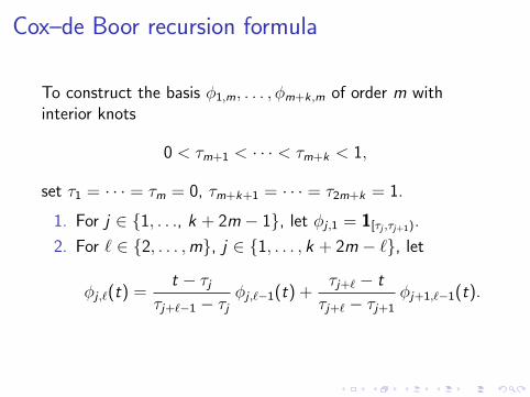
Cox–de Boor recursion formula
To construct the basis φ1,m, . . . , φm+k,m of order m withinterior knots
0 < τm+1 < · · · < τm+k < 1,
set τ1 = · · · = τm = 0, τm+k+1 = · · · = τ2m+k = 1.
1. For j ∈ {1, . . ., k + 2m − 1}, let φj ,1 = 1[τj ,τj+1).
2. For ` ∈ {2, . . . ,m}, j ∈ {1, . . . , k + 2m − `}, let
φj ,`(t) =t − τj
τj+`−1 − τjφj ,`−1(t) +
τj+` − t
τj+` − τj+1φj+1,`−1(t).

Illustration: Third-order B-spline basis
0.0 0.2 0.4 0.6 0.8 1.0
0.0
0.2
0.4
0.6
0.8
1.0
t
B−
splin
e
This basis has k = 4 equally-spaced interior knots and consistsof m + k = 7 B-spline polynomials of degree m − 1 = 2.

Fitting procedure
Assume that for unknown β = (β1, . . . , βm+k)>,
∀t∈[0,1] A(t) =m+k∑j=1
βjφj ,m(t) = β>Φ(t),
where Φ(t) = (φ1,m(t), . . . , φm+k,m(t))>.
View this as a regression E(Z ) = β>X for which we have data
(X1,Y1) = (Φ(T1),Z1), . . . , (Xn,Yn) = (Φ(Tn),Zn).
with Ti = ln(Vi)/ln(Ui Vi), Zi = ln{Cn(Ui , Vi)}/ln(Ui Vi).
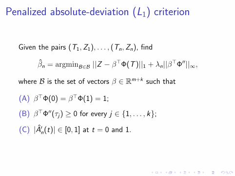
Penalized absolute-deviation (L1) criterion
Given the pairs (T1,Z1), . . . , (Tn,Zn), find
βn = argminB∈B ||Z − β>Φ(T )||1 + λn||β>Φ′′||∞,
where B is the set of vectors β ∈ Rm+k such that
(A) β>Φ(0) = β>Φ(1) = 1;
(B) β>Φ′′(τj) ≥ 0 for every j ∈ {1, . . . , k};
(C) |A′n(t)| ∈ [0, 1] at t = 0 and 1.

Technical details
(A)–(C) guarantee that An is intrinsic if m ∈ {3, 4} becauseA′′n is then linear between the knots. Hence
∀j∈{1,...,m} β>Φ′′(τj) ≥ 0 ⇒ ∀t∈(0,1) A′′n(t) ≥ 0.
The penalization term λn||β>Φ′′||∞ is needed to make thesolution smooth when the knots are unknown (always!).
Minimization is performed over a large number of equallyspaced empirical quantiles derived from T1, . . . ,Tn.
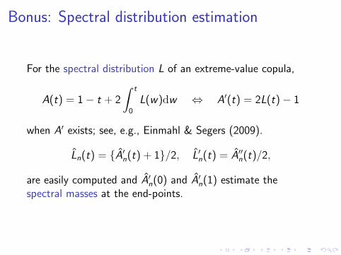
Bonus: Spectral distribution estimation
For the spectral distribution L of an extreme-value copula,
A(t) = 1− t + 2
∫ t
0
L(w)dw ⇔ A′(t) = 2L(t)− 1
when A′ exists; see, e.g., Einmahl & Segers (2009).
Ln(t) = {A′n(t) + 1}/2, L′n(t) = A′′n(t)/2,
are easily computed and A′n(0) and A′n(1) estimate thespectral masses at the end-points.
Computer implementation (m = 3)
X The procedure is coded in R using the “COBS” package.
X It is fully automated and only requires the user to definethe constraints and the number of knots.
X From experience, between 10 and 15 knots suffice tocapture the complexity of the data.
X The derivatives are calculated using the “FDA” packageafter knot and coefficient abstractions from “COBS”.
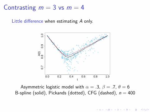
Contrasting m = 3 vs m = 4
Little difference when estimating A only.
●
●
●
●
●
●●
●
●
●
●
●
●
●
●
●
●
●
●
● ●
●
●
●
●
●
● ●
●
●
●
●
●
●
●
●
●
●
●
●
●
●
●
●
●
●
●
●
●●
●
●
●
●
●
●
●
●
● ●
●
●
●
●
● ●
●
●
●
●
●
●
●
●
●
●
●
●
●
●●
●
●
●
●●
●
●
●
●
●
●
● ●
●
●
●
●
●
●
●
●
●
●
●
●●
●
●
●
●●
●
●
●
●
●
●
●●
●●
●
●
●
●
●
●
●
●
●
●
●
●
●
●
●
●●
●
●
●
●
●
●
●
●
●
●
●●
●
●
●
●
●
●
●
●
●
●
●
●
●
●
●
●
●
●●
●
●
●
●
●●
●
●●
●
●
●
●
●
●
●
●
●
●
●
●
●
●
●
●
●
●
●
●
●
●
●
●
●
●
●
●
●●
●
●
●
●
●
●
●
●
●
●
●
●
●
●
●
●
●
●
●
●
●
●
●
●●
●
●
●
●
●
●●
●
●
●
●
●
●
●
●
●
●
●
●●
●
●
●
●
●
●
●
●
●
●
●
●
●
●
●
●
●
●
●
●
●
●
●
●
●
●
●
●
●
●
●
●●●
●
●
●
●
●
●
●
●
●
●
●
●
●
●
●
●
●
●
●
●
●●
●
●
●
●
●
●
●
●
●
●
●
●
●
●
●
●
●
●
●
●
●
●
●
●
●
●
●
●
●
●
●
●
●
●
●
●
●●
●
●
●
●
●
●
●
●
●
●
●
●
●
●
●
●
●
●
●
●
●
●
●
●
●
●
●
●
●
●
●
●
●
●
●
●
●
●
●
●
●
●
●
●
●
●
●
●
●
●
●
●
0.0 0.2 0.4 0.6 0.8 1.0
0.7
0.8
0.9
1.0
t
A(t
)
Asymmetric logistic model with α = .3, β = .7, θ = 6B-spline (solid), Pickands (dotted), CFG (dashed), n = 400
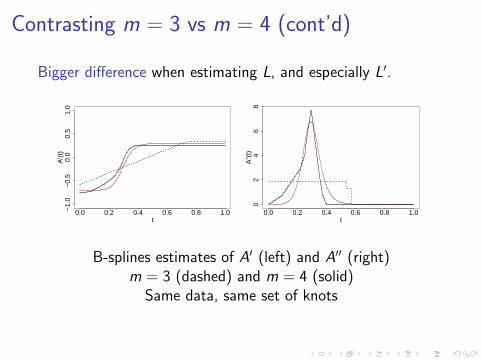
Contrasting m = 3 vs m = 4 (cont’d)
Bigger difference when estimating L, and especially L′.
0.0 0.2 0.4 0.6 0.8 1.0−1.
0−
0.5
0.0
0.5
1.0
t
A'(t
)
0.0 0.2 0.4 0.6 0.8 1.0
02
46
8
t
A''(
t)
B-splines estimates of A′ (left) and A′′ (right)m = 3 (dashed) and m = 4 (solid)
Same data, same set of knots

5. Simulation results and data illustration
The B-spline estimators of L with m = 3 and m = 4 werecompared to the estimator of Einmahl & Segers (2009).
X 9 extreme-value and 5 other copulas;
X various degrees of asymmetry and dependence;
X various sample sizes and N = 1000 repetitions.
Performance measure used:
Dn =1
n
n∑i=1
{L(Ti)− Ln(Ti)}2.
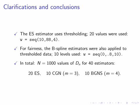
Clarifications and conclusions
X The ES estimator uses thresholding; 20 values were used:w = seq(10,88,4).
X For fairness, the B-spline estimators were also applied tothresholded data; 10 levels used: w = seq(0,.8,10).
X In total: N = 1000 values of Dn for 40 estimators:
20 ES, 10 CGN (m = 3), 10 BGNS (m = 4).
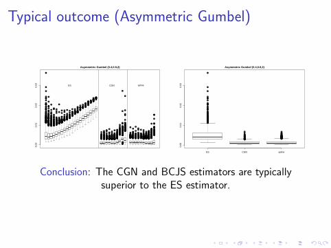
Typical outcome (Asymmetric Gumbel)
●
●
●
●●●●
●
●
●
●
●
●
●
●
●
●
●
●
●
●●●
●
●
●
●
●
●
●
●
●
●
●●●●●●
●
●●
●
●
●
●
●●●
●
●
●
●
●●
●
●
●
●
●
●
●
●
●
●
●
●●
●
●
●
● ●
●
●
●●●●
●
●
●●
●
●
●
●
●
●
●●●●●
●
●
●
●
●●
●
●●
●
●●●●
●
●
●
●
●
●●
●
●●
●
●
●●
●
●
●●●
●
●●
●
●
●
●
●
●
●
●
●
●●●
●
●●
●
●
●
●
●
●
●●
●●
●
●
●
●●
●●●
●
●●
●
●
●
●
●
●
●●●
●
●
●
●
●●
●
●
●
●
●●●
●
●
●
●
●
●
●
●
●●
●
●●●
●
●
●●
●●●
●
●●
●
●
●
●
●
●●
●
●
●
●
●●●●●● ●
●
●
●●
●
●●●
●●
●
●
●●●
●
●
●
●
●●●
●●●
●
●●●●
●
●
●
●
●●●
●
●●●● ●
●
●
●
●
●
●●●●●●●
●●●
●
●●●●
●
●
●
●●
●
●
●
●●●●●
●
●●●●
●
●●
●
●●●●
●
●●●
●●
●●
●
●●●●
●
●
●
●●●●●●●
●
●●●●
●●●●●●
●
●●
●●
●●
●
●●●
●
●●●
●
●
●●●●
●
●●●●
●
●●●●
●
●●●●●
●
●
●●●●●●●
●
●●●
●●●
●●●●
●
●
●●
●
●
●
●
●●●●
●
●
●●●●
●●
●
●
●●●●●●
●●●●
●●
●
●
●●●●●
●●
●●●●
●
●●●
●
●●
●●
●●
●
●
●
●
●●●●●●●●●●●
●
●●●●●
●
●
●●
●●●●
●
●●
●●●●
●
●
●
●●●●●
● ●●●●●●●●●●●
●●●●●●●●●●●●●
●●●●●●●●●●●
●●●●
●
●●●
●●●●●
●●●●●●
●
●●●●●
●
●●●●
●●●●
●●
●●●●
●●●●●●
●
●●●●●
●
●●●●●●
●●
●
●
●
●
●●
●●
●●
●●●●●●●
●
●●●●●●●●
●●
●●●●●●●●●
●
●●
●
●●
● ●●●●
●●●●●
●●
●●●●
●
●●●●●
●
●●●●●●●●●
●
●●
●
●●●●●●
●●●
●●
●
●●●●
●● ●
●●
●●●●●
●
●●●
●
●
●●●●●●●
●
●●●●●●●
●●
●●●●●●●
●●● ●●
●●●●●●●
●●
●
●
●●●●●●
●●●●●●●●
●●●●●
●
●
●● ●
●●●●●
●
●●●●●●
●
●
●
●
●●
●
●●●●●●●
●
●
●
●●●
●●
●●●
●
●●●
●●●●
●
●
●
●●●
●● ●●
●
●
●
●
●●●●●●
●
●●●●
●
●
●
●●●●●●●●●●●
●●●
●●
●●
●●●●●
●●
●
●●●
●●●
●
●●
● ●●●
●●
●
●
●
●●
●
●●●●
●
●
●●●
●
●
●
●
●
●
●●●
●
●●●●●●
●
●
●
●●●
●
●●
●
●●●
●
●●●●
●●●●●
●
●●
●
●
●
●
●
●●
●●
●
●
●
●
●
●
●
●
●
●
●●
●
●●●
●●
●
●
●●●
●
●
●●
●●
●●
●●
●
●●●●
●
●
●●
●
●
●●
●●
●
●
●●●●
●●
●
●
●
●
●
●
●●●●
●
●
●
●
●
●●
●
●●
●
●●
●
●●
●●●
●
●
●
●●●
●
●●●
●
●
●
●
●
●●●●
●
●
●●●
●●●●●
●
●●●●
●●●●
●
●●
●
●
●●
●●●●●●●●●●●
●●●●
●
●●●●●
●●●●●●●●●
●●●
●
●●
●
●
●
●●
●
●
●●●●●●
●
●●●●●●●●●
●●
●
●●
●
●●●
●
●
●●●●●●● ●
●●●●●●●●●
●●●●●●●
●
●●
●●●
●
●●●●●●
●●
●
●●●●●●
●●●●●●
●
●
●●
●●●●●
●●●
●●● ●●●●
●●
●●●
●
●
●
●●●●●
●
●●
●
●●●●
●
●●
●
●
●●
●●●
●● ●
●
●●●●●●●●●
●●●●
●●
●
●
●●●●
●
●●●●●●
●
●
●●
●
●
● ●●
●●●
●
●●
●●●●
●
●●
●
●
●●●●●●
●
●●●●●●●
●●
●●●●
●
●●●●
●
●
●
●
●
●●●
●
●
●
●
●
●
●●●●●●
●
●●●
●
●
●
●
●
●●
●●●
●
●●●●
●
●●
●●●●●
●
●
●●
●
●●
●
●●●
●
●
●●●
●
●●
●
●
●
●
●●
●
●
●
●
●
●
●
●
●
●●
●
●
●
●●
●
●
●●
●
●●
●
●
●
●
●
●●
●●
●●
●
●
●
●
●
●
●
●●
●●
●
●
●
●
●●
●
●
●
●
●
●
●
●
●
●
●
●●
●
●
●
●●●●●●
●
●●●
●
●●
●
●
●●
●
●●
●
●
●●
●●●
●
●
●●
●●
●
●●
●
●
●
●
●
●
●
●●
●
●
●
●
●
●●
●
●●●
●
●
●
●
●●
●
●
●
●
●
●
●
●
●
●●
●
●
●
●
●
●●
●●●
●●●
●●●●●
●
●
●●
●●
●
●
●
●
●
●
●
0.00
0.01
0.02
0.03
Asymmetric Gumbel (0.4,0.8,2)
ES CGN spline
●
●
●
●●●●
●
●
●
●
●
●
●
●
●
●
●
●
●
●●●
●
●
●
●
●
●
●
●
●
●
●●●●●●
●
●●
●
●
●
●
●●●
●
●
●
●
●●
●
●
●
●
●
●
●
●
●
●
●
●●
●
●
●
●
●●
●●●●●●●●●
●●●●
●●
●
●
●●●●
●
●●●●●●
●
●
●●
●
●
● ●●
●
●
●
●
●●●●●●
●
●●●●
●
●
●
●●●●●●●●●●●
●●●
●●
●●
●●●●●
●●
●
●●●
●●●
●
●●
●
ES CGN spline
0.00
0.01
0.02
0.03
Asymmetric Gumbel (0.4,0.8,2)
Conclusion: The CGN and BCJS estimators are typicallysuperior to the ES estimator.

Danish Fire Insurance Data
0.0 0.2 0.4 0.6 0.8 1.0
0.0
0.2
0.4
0.6
0.8
1.0
buliding
contents
0.0 0.2 0.4 0.6 0.8 1.0
0.0
0.2
0.4
0.6
0.8
1.0
buliding
profits
0.0 0.2 0.4 0.6 0.8 1.0
0.0
0.2
0.4
0.6
0.8
1.0
contents
profits
0.0 0.2 0.4 0.6 0.8 1.0
0.5
1.0
1.5
2.0
t
A(t)
0.0 0.2 0.4 0.6 0.8 1.0
0.6
0.8
1.0
1.2
t
A(t)
0.0 0.2 0.4 0.6 0.8 1.0
0.5
0.6
0.7
0.8
0.9
1.0
tA(t)
(X ,Y ), (X ,Z ), (Y ,Z )
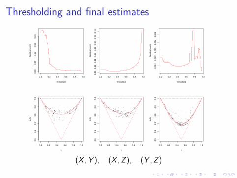
Thresholding and final estimates
0.0 0.2 0.4 0.6 0.8 1.0
0.00
0.01
0.02
0.03
0.04
Threshold
Re
sid
ua
l e
rro
r
0.0 0.2 0.4 0.6 0.8 1.0
0.000.020.040.060.080.100.120.14
Threshold
Re
sid
ua
l e
rro
r
0.0 0.2 0.4 0.6 0.8 1.0
0.001
0.002
0.003
0.004
0.005
Threshold
Re
sid
ua
l e
rro
r
0.0 0.2 0.4 0.6 0.8 1.0
0.5
0.6
0.7
0.8
0.9
1.0
t
A(t)
0.0 0.2 0.4 0.6 0.8 1.0
0.5
0.6
0.7
0.8
0.9
1.0
t
A(t)
0.0 0.2 0.4 0.6 0.8 1.0
0.5
0.6
0.7
0.8
0.9
1.0
tA(t)
(X ,Y ), (X ,Z ), (Y ,Z )

Take-home message
X The A-plot is useful for detecting extreme-valuedependence.
X An intrinsic estimator of A can be based on B-splines.
X B-splines of order m = 3 are adequate for estimating A(off-the-shelf solution with COBS and FDA packages).
X B-splines of order m = 4 yield better estimates of L andL′ than the approach of Einmahl & Segers (2009).
X Asymptotic theory is available and non-extreme data canbe handled via thresholding (no asymptotics in support).

Research funded by