Estimating andSimulating a SIRDModel ofCOVID ...web.stanford.edu/~chadj/sird-paper.pdfdemographic and selection-into-disease mechanism, which are themselves partly the product of endogenous

Estimating and Simulating a SIRD Model

of COVID-19 for Many Countries, States, and Cities

Jesus Fernandez-Villaverde Charles I. Jones∗

UPenn and NBER Stanford GSB and NBER

May 29, 2020 — Version 2.01

Abstract

We use data on deaths in New York City, Madrid, Stockholm, and other world

cities as well as in various U.S. states and various countries and regions to estimate

a standard epidemiological model of COVID-19. We allow for a time-varying con-

tact rate in order to capture behavioral and policy-induced changes associated with

social distancing. We simulate the model forward to consider possible futures for

various countries, states, and cities, including the potential impact of herd immu-

nity on re-opening. Our current baseline mortality rate (IFR) is assumed to be 1.0%

but we recognize there is substantial uncertainty about this number. Our model

fits the death data equally well with alternative mortality rates of 0.5% or 1.2%, so

this parameter is unidentified in our data. However, its value matters enormously

for the extent to which various places can relax social distancing without spurring

a resurgence of deaths.

∗We are grateful to Leopold Aschenbrenner, Adrien Auclert, John Cochrane, Sebastian Di Tella, GlennEllison, Bob Hall, Pete Klenow, Chris Tonetti, Giorgio Topa, Eran Yashiv, and to participants at the Stanfordmacro lunch for helpful comments and to Ryan Zalla for excellent research assistance. A dashboardcontaining results for around 100 countries, states, and cities can be found on our web page, here.

http://web.stanford.edu/people/chadj/Covid/Dashboard.html

ESTIMATING AND SIMULATING A SIRD MODEL 1

Change log:

– May 29, 2020: Version 2.0: Drop the “exponential decay” model of βt. Instead, invert

the SIRD model and use death data to recover a βt and therefore R0t = βt/γ at each

date. For simulations of future outcomes, allow for feedback from daily deaths, dt, to

future behavior according to R0t = Constant ·e−αdt as suggested by Cochrane (2020).

– May 2, 2020: Version 1.0 (NBER working paper). Updated graphs and added a log

scale graph of cumulative deaths

– April 28, 2020: Version 0.6: updated based on random testing in New York to a bench-

mark mortality rate (IFR) of 0.8% and data through April 24. Uses a SIRDC model

with 5 states and an “exponential decay” model of βt.

– April 23, 2020: Version 0.5, first public version, based on a benchmark mortality rate

(IFR) of 0.3% and data through April 21.

1. Introduction

We use data on deaths in New York City, Madrid, Stockholm, and other world cities

as well as in various U.S. states, countries, and regions around the world to estimate

a standard epidemiological model of COVID-19. Relative to existing frameworks, our

contributions are

• We do not use data on cases or tests because of differential selection in testing in

different cities, states, and countries. Instead we only use data on deaths.

• We invert a standard SIRD epidemiological model and use the daily death series

to recover a time-varying R0t ≡ βt/γ to capture changes in behavior and policy

that occur at different times and with different intensities in different locations. In

essence, we apply a Solow residual approach: we assume the model fits the data

exactly and back out the implied values of βt that make it so. Relative to our earlier

“exponential decay” approach, this formulation has the advantage of being able

to capture re-opening effects that may increase contacts.

• We show how simulating our model after a location has reached a peak in the

number of daily deaths results in very stable results going forward in time. In

2 FERNANDEZ-VILLAVERDE AND JONES

contrast, simulations of the future before a location reaches its peak are extremely

noisy and sensitive to daily shocks.

• For simulations of future outcomes, we allow for feedback from daily deaths, dt,

to future behavior according to R0t = Constant · e−αdt as suggested by Cochrane

(2020). We estimate α from data for each country. There is tremendous hetero-

geneity across countries, so this parameter is not well-identified in our data. We

estimate an average value of about α = 0.05 so that R0 changes by 5% when daily

deaths change by one and use this value in simulations of future outcomes.

• Our models allow us to back out the percent of people who are currently in-

fectious as well as who are ever-infected versus still susceptible and therefore

estimate the extent to which herd immunity effects are large. We find moder-

ate effects in New York City, noticeable effects in Italy, Sweden, and Spain, and

negligible effects in New York state outside of New York City and in places like

California.

We are not epidemiologists, so these results should be interpreted with caution

and care. We study a standard model of COVID-19 using common tools in econo-

metrics and then analyze its main quantitative implications in ways that resemble how

economists study other dynamic models. Our exercise can help us understand where

a simple SIRD model has difficulties fitting observed patterns in the data and points

out avenues for improvement while maintaining the virtues of simplicity and parsi-

mony. We plan to update these results regularly on our dashboard, where we also report

around 25 pages of graphs for each of around 100 cities, states, and countries.

2. Literature Review

Much of the mathematical study of the spread of infectious diseases start from the

classic compartmental models of Kermack and McKendrick (1927) and Kermack and

McKendrick (1932). These models divide the population into several different com-

partments (e.g., susceptible, infective, recovered, deceased, ...) and specify how agents

https://web.stanford.edu/~chadj/Covid/Dashboardhtml


move across the separate compartments over time.1 The SIRD epidemic model that we

analyze in this paper is one of the simplest of these compartmental models. Hethcote

(2000) presents a useful overview of this class of models and some of their theoretical

properties and Morton and Wickwire (1974) shows how to apply optimal control meth-

ods to them. Also, Brauer, Castillo-Chavez and Feng (2019) is a recent, comprehensive

textbook of the field and Imperial College COVID-19 Response Team (2020) is an exam-

ple of how these models have been applied to understand the current health crisis by

epidemiologists.

The acute economic impact of the current pandemic has generated much interest

among economists in exploring compartmental models and how they can be dove-

tailed into standard economic models and estimated using econometric techniques.

(see Stock, 2020, and Avery et al., 2020, for two general surveys of how economists have

addressed this topic).

First, economists have argued that many of the parameters controlling the move

among compartments are not structural in the sense of Hurwicz (1962), but depend,

instead, on individual decisions and policies. For example, the rate of contact that

determines the number of new infections is a function of the endogenous labor supply

and consumption choices of individuals. Hence, the rate of contact is amenable to be

studied with standard decision theory models. See, for instance, Eichenbaum, Rebelo

and Trabandt (2020) and Farboodi, Jarosch and Shimer (2020). Also, the recovery and

death rates are not just clinical parameters, but can be functions of policy decisions

such as expanded emergency hospital capacity or priorities regarding the allocation

of scarce ICU resources. Similarly, the case fatality ratio, a key figure to assess the

severity of the epidemic, is a complex function of clinical factors (e.g., the severity of a

virus) and demographic and selection-into-disease mechanism, which are themselves

partly the product of endogenous choices (Korolev, 2020b).2 Our paper builds on these

ideas by allowing the infection rates to be influenced by social distancing and by letting

many parameters to vary across countries, states, and cities, which can proxies for

demographic and policy heterogeneity.

1Before the contributions of Kermack and McKendrick, William Farr (1807-1883) had observed thatepidemics tend to follow a Gaussian curve; however, he never presented a formal mechanism to accountfor such a pattern.

2More precisely, the case fatality ratio is not the average treatment effect on the treated (ATET), a moreexplicitly “causal” concept.


Second, economists have been concerned with the identification problems of com-

partmental models. Many of these models are unidentified or weakly identified, with

many set of parameters that fit the observed data so far equally well but have consider-

ably different long-run consequences. Atkeson (2020) and Korolev (2020a) document

this argument more carefully. Our findings corroborate this result and highlight the

need to develop alternative econometric approaches.

Third, some researchers have dropped the use of compartmental models completely.

Instead, they have relied on time-series models from the econometric tradition. See, for

instance, Linton (2020), Kucinskas (2020), and Liu, Moon and Schorfheide (2020).

Let us close this section by pointing out that economists are pushing the study

of compartmental models in a multitude of dimensions. Acemoglu, Chernozhukov,

Werning and Whinston (2020), Alvarez, Argente and Lippi (2020), and Chari, Kirpalani

and Phelan (2020) characterize the optimal lockdown policy for a planner who wants to

control the fatalities of a pandemic while minimizing the output costs of the lockdown.

Berger, Herkenhoff and Mongey (2020) analyze the role of testing and case-dependent

quarantines. Bethune and Korinek (2020) estimate the infection externalities associ-

ated with COVID-19 and find them to be large. Bodenstein, Corsetti and Guerrieri

(2020) combine a compartmental model with a multisector dynamic general equilib-

rium model to capture key characteristics of the U.S. Input-Output Tables. Garriga,

Manuelli and Sanghi (2020), Hornstein (2020), and Karin, Bar-On, Milo, Katzir, Mayo,

Korem, Dudovich, Yashiv, Zehavi, Davidovich et al. (2020) study a variety of contain-

ment policies. Toda (2020), besides also estimating a SIRD model as we do, explores

the optimal mitigation policy that controls the timing and intensity of social distancing.

More papers are appearing every day.

3. A SIRD Model with Social Distancing

We follow standard notation in the literature. There is a constant population of N

people, each of whom may be in one of five states:

St + It +Rt +Dt + Ct = N

The states — in temporal order — are


St = Susceptible

It = Infectious

Rt = Resolving

Dt = Dead

Ct = ReCovered

A susceptible person contracts the disease by coming into “adequate” contact with

an infectious person, assumed to occur at rate βtIt/N , where βt is a time-varying con-

tact rate parameter.

The starting value of βt, β0, reflects how the infection would progress if individuals

were behaving as they did before any news of the disease had arrived. We think of β0 as

capturing characteristics of the disease, fixed attributes of the region such as density,

and basic customs in the region.

Over time, βt varies depending on how strong is the social distancing and hygienic

practices that different locations adopt, either because of policy or simply because of

voluntary changes in individual behavior. We will explain below how we recover βt from

the data but, at this moment, we are not imposing any structure on its evolution.3

The total number of new infections at a point in time is βtIt/N · St. Infectiousness

resolves at Poisson rate γ, so the average number of days a person is infectious is 1/γ:

e.g., γ = .2 ⇒ 5 days.

After the infectious period is over, a person is in the “Resolving” state, R. A constant

fraction, θ, of people exit this state each period, and the case is resolved in one of two

ways:

Death: fraction δ

Recovery: fraction 1− δ

In earlier versions of this project, we found that it is important to have a model that

distinguishes between the infectious and the recovering periods. This distinction was

key to matching the data with biologically plausible parameter values when we were

putting restrictions on the time path of βt. In particular, it appears that the infectious

period lasts on average about 4 to 5 days while cases take a total of about 2 to 3 weeks

3In a previous version of this paper, we imposed that βt decayed at an exponential rate, as assumed,for example, in Chowell, Viboud, Simonsen and Moghadas (2016). We also tried alternative specifications,including discrete jumps at the time of the introduction of shelter-in-place orders. As we will see below, itturns out that we can dispense from those assumptions and be much more flexible in recovering βt fromobservables.


or even longer to resolve (Bar-On et al., 2020).4 If one assumes people are infectious for

this entire period, the model has trouble fitting the data.

The laws of motion related to the virus are then given by

∆St+1 = −βtStIt/N︸︷︷︸

new infections

(1)

∆It+1 = βtStIt/N︸︷︷︸

new infections

− γIt︸︷︷︸

resolving infectious

(2)

∆Rt+1 = γIt︸︷︷︸

resolving infectious

− θRt︸︷︷︸

cases that resolve

(3)

∆Dt+1 = δθRt︸︷︷︸

die

(4)

∆Ct+1 = (1− δ)θRt︸︷︷︸

reCovered

(5)

We assume the initial stocks of deaths are set equal to zero. The initial stock of infec-

tions and resolving cases, I(0) and R(0), are parameters that we will estimate.

3.1 Basic Properties of a Standard SIRD Model

Here we review the basic properties of this model when βt = β and the difference

equations are replaced by differential equations (Hethcote, 2000). A convention in epi-

demiological modeling is to recycle notation and let R0 denote the basic reproduction

number, that is, the expected number of infections generated by the first ill person

when s0 ≡ S0/N ≈ 1:

R0 = β × 1/γ

# of infections

from one sick

person

# of lengthy

contacts per

day

# of days

contacts are

infectious

More generally, if R0s0 > 1, the disease spreads, otherwise it declines quickly. One

can see from this simple equation why R0 > 1 is so natural: if people are infectious for

4We can also consider the transition to the resolving compartment as reflecting, in part, quarantinemeasures. While some authors prefer to add a “quarantine” compartment, we did not find we needed it toaccount for the dynamics of the data.


5 days and have lengthy contacts with even just two new people per day, for example,

then R0 = 10.

As shown by Hethcote (2000), the initial exponential growth rate of infections is β −

γ = γ (R0−1). Another useful result from these models concerns the long-run number

of people who ever get infected (and therefore the fraction δ of these gives the long-run

death rate). As t → ∞, the total fraction of people ever infected, e∗, solves (assuming

s0 ≈ 1)

e∗ = −1

R0

log(1− e∗)

In other words, with a constantβ, the long run number of people ever infected is pinned

down by R0; the parameters γ and θ only affect the timing, holding R0 constant. The

long-run death rate is then δe∗, so this too depends only on R0 (and δ).

This explains why modeling the changing β associated with social distancing and

better hygienic practices is so important. With a constant β, the initial explosion rate of

the disease implies a value for β and then all the variables in the differential system are

determined at that point. Instead, a changing β permits the initial exponential growth

rate of deaths to be different from the long-run properties of the system, which is the

point of adopting behavioral changes in society.

4. Recovering βt and therefore R0t

It turns out that recovering βt, a latent variable, from the data is straightforward without

having to resort to any complex filtering device.

We adopt the following timing convention. Dt+1 is the stock of people who have

died as of the end of date t+ 1, so that ∆Dt+1 ≡ dt+1 is the number of people who died

on date t+ 1 (daily deaths, in our estimating exercise).

We begin by using equation (4) to solve for various series involving Rt+1 and its

differences in terms of daily deaths:

Rt =1

δθ∆Dt+1 =

1

δθdt+1 (6)

∆Rt+1 =1

δθ(dt+2 − dt+1) =

1

δθ∆dt+2 (7)

Next, we use (3) and the expressions we just derived for Rt+1 to solve for It and its


differences:

It =1

γ(∆Rt+1 + θRt) (8)

=1

γ

(∆dt+2

δθ+ dt+1/δ

)

(9)

=1

δγ

(∆dt+2

θ+ dt+1

)

(10)

and applying the difference operator gives:

∆It+1 =1

δγ

[∆dt+3 −∆dt+2

θ+∆dt+2

]

(11)

=1

δγ

(∆∆dt+3

θ+∆dt+2

)

(12)

where ∆∆dt+3 ≡ ∆dt+3 −∆dt+2.

Taking the ratio of (12) to (10) gives:

∆It+1

It=

1

θ∆∆dt+3 +∆dt+2

1

θ∆dt+2 + dt+1

(13)

Now, we can go back to our original SIRD model in equation (2) and rewrite it as

∆It+1

It= βt

St

N− γ

Solve this equation for βt by using equation (13) above to get

βt =N

St

(

γ +∆It+1

It

)

=N

St

(

γ +1

θ∆∆dt+3 +∆dt+2

1

θ∆dt+2 + dt+1

)

(14)

This is one of the key equations in recovering βt. Notice, however, that this equation

depends on St. But since we have an initial condition for S0, we can use the SIRD model

to get the updating equation for ∆St+1 and we will be done. From (1) and using (10) to

substitute It:

∆St+1 = −βtSt

ItN


= −βtSt

1

δγN

(1

θ∆dt+2 + dt+1

)

(15)

or

St+1 = St

(

1− βt1

δγN

(1

θ∆dt+2 + dt+1

))

(16)

Now we only need to collect the last two equations together:

βt =N

St

(

γ +1

θ∆∆dt+3 +∆dt+2

1

θ∆dt+2 + dt+1

)

(17)

and:

St+1 = St

(

1− βt1

δγN

(1

θ∆dt+2 + dt+1

))

. (18)

With these two equations, an observed time series for daily deaths, dt, and an initial

condition S0/N ≈ 1, we iterate forward in time and recover βt and St+1. Basically, we

are using future deaths over the subsequent 3 days to tell us about βt today. While this

means our estimates will be three days late (if we have death data for 30 days, we can

only solve for β for the first 27 days), we can still generate an informative estimate of βt.

There are many exercises we can perform with the recovered βt. We can, for in-

stance, simulate the model forward using the most recent value of βT and gauge where

a region is headed in terms of the infection and current behavior. And we can corre-

late the βt with other observables to evaluate the effectiveness of certain government

policies such as mandated lock downs.

Note, also, that βt determines the basic reproduction number, R0t = βt× 1/γ under

the current social distancing and hygienic practices. We should be careful to distin-

guish this basic reproduction number from the effective reproduction number (i.e.,

the average number of new infections caused by a single infected individual at time

t), which we will denote by Ret. The latter considers the fraction of the population that

is still susceptible. Since:

Ret = R0t · St/N,

our procedure can also recover the effective reproduction number. This finding is in-

teresting because this effective reproduction number is often reported by researchers


due to the easiness with which it can be estimated with standard statistical packages

such as EpiEstim in R.

5. Estimation: Countries and States

The following parameters are assumed to be primarily biological and, therefore, fixed

over time and the same in all countries and regions:

• γ = 0.2: In the continuous time version of this model, the average length of time

a person is infectious is 1/γ, so 5 days in our baseline. This choice is consistent

with the evidence in Bar-On, Flamholz, Phillips and Milo (2020). We also consider

γ = 0.15 (7 day duration). The γ = 0.2 fit slightly better in our earlier work with

more restrictions on βt, but it was not particularly well identified.5

• θ = 0.1: In the continuous time version of this model, the average length of time it

takes for a case to resolve, after the infectious period ends, is 1/θ. With θ = .1, this

period averages 10 days. Combined with the 5-day infectious period, this implies

that the average case takes a total of 15 days to resolve. The implied exponential

distribution includes a long tail that can be thought of as capturing the fact that

some cases take even longer to resolve.

• α = 0.05: For simulations of future outcomes, we allow for feedback from daily

deaths per million people, dt, to future behavior according to R0t = Constant ·

e−αdt as suggested by Cochrane (2020). We estimateαi from data for each location

i. There is tremendous heterogeneity across locations in these estimates, so a

common value is not well-identified in our data. We estimate an average value

of about α = 0.05 so that R0t changes by 5% when daily deaths change by one.

This is the value we use in simulations of future outcomes. More specifically, the

mean value of αi in location-specific regressions is 0.066 and the median value is

0.045. However, the standard deviation of αi across locations is a very high 0.15.

We report results with both α = 0 — i.e., assuming no feedback so that the final

5Note that γ also incorporates choices of individuals and that, therefore, it is not merely pinneddown by clinical observations. If an individual experiences symptoms or is suspicious that she mightbe infectious, hence withdrawing herself from effective contacts with susceptible individuals, we canconsider her case has resolved for the purposes of the dynamics of the model, even if she is still undera clinical condition.


value of R0t that we estimate in the data is assumed to hold in the future — as

well as with α = .05. The presence of feedback is very clear in our estimation and

strikes us as helpful to incorporate, so our baseline results below assume α = .05.

• δ = 1.0%: This parameter is crucial, and it would be great to have a precise

estimate of it. Case fatality rates are not helpful, as we do not have a good measure

of how many people are infected. Random testing for antibodies to detect how

many people have ever been infected is quite informative about this parameter.

The most comprehensive evidence we are aware of comes from a seroepidemio-

logical national survey undertaken by the Spanish Government from April 27 to

May 11 to measure the incidence of SARs-CoV-2 in Spain.6 The survey was large,

with 60,983 valid responses from individuals stratified in two stages. Combining

the results from this survey with the measured sensitivity and specificity of the

test, we conclude that the mortality rate of SARs-CoV-2 in Spain is between 1%

and 1.1%. Because many of the early deaths in the epidemic were linked with

mismanagement of care at nursing homes in Madrid and Barcelona that could

have been avoided, we pick 1% as our benchmark value.

Since mortality rates are affected by the demographic composition of the popu-

lation (with COVID-19 mortality rates increasing sharply with age), we obtained

data on age distributions across countries from the U.N. population division. We

decomposed the Spanish mortality rate by age, given the age-specific measured

infection incidence rates, and applied those age-mortality rates to the population

shares of each country. To control for differences in life expectancy (and hence,

for the possibility that the age-specific mortality rate of an 80-year-old individual

in a high life-expectancy country is equivalent to the age-specific mortality rate of

a 70-year-old individual in a low life-expectancy country), we applied a correction

based on the ratio of the life expectancy of each country with respect to Spain’s life

expectancy.

We found that, for most of the countries in our sample, the estimated mortality

rate clusters around 1% (with or without the correction by life expectancy). For

example, for the U.S., we found a death rate of 0.76% without correcting for life ex-

6Preliminary report available at https://www.ciencia.gob.es/stfls/MICINN/Ministerio/FICHEROS/ENECOVIDInforme preliminar cierre primera ronda 13Mayo2020.pdf.

https://www.ciencia.gob.es/stfls/MICINN/Ministerio/FICHEROS/ENECOVID_Informe_preliminar_cierre_primera_ronda_13Mayo2020.pdf


pectancy and 1.05% correcting by it. Therefore, and parsimoniously, we selected

1% as our baseline parameter values.

Other studies suggest similar values of δ. For instance, on April 23, Governor An-

drew Cuomo announced preliminary results suggesting that 21% of New York City

residents randomly tested from supermarkets and big-box stores had antibodies

for COVID-19. According to New York Department of Health (2020), it takes 3-4

weeks for these antibodies to form, so this suggests that around April 1, 21% of

NYC residents were “ever infected.” This infection rate is consistent with back-of-

the-envelope calculations of death rates of around 0.8%-1%.

Some earlier papers had estimated values of the death rate as low as 0.3%, a value

we used in a previous draft of this paper. For instance, Hortasu, Liu and Schwieg

(2020) report an IFR of 0.3% using data on travelers from Iceland and some more

limited serological studies in Santa Clara County, Los Angeles, and Heinsberg

(Germany) also pointed out to death rates between 0.3% and 0.4%. However,

some of these studies were criticized for not accounting for the sensibility of test-

ing or were not stratified properly. The current updated evidence suggests that

death rates lower than 0.8% are unlikely. Thus, we will report robustness results

using death rates of 0.8% and 1.2%.

Data. Our data are taken from the GitHub repository of Johns Hopkins Univer-

sity CSSE (2020), which reports cumulative death numbers daily for countries,

states, counties, and provinces throughout the world. The exception is for the

international cities/regions of Lombardy, London, Madrid, Stockholm, and Paris.

We obtain data for these locations of the various national vital statistics agencies.

We manipulate this data in three important ways before feeding it into the model.

First, on April 15, New York City added more than 3,500 deaths to their counts,

increasing the total by more than 43%. We therefore apply this same factor of pro-

portionality (1.4325) to the deaths before April 15 to get a consistent time series

for New York City. Second, The Economist (2020) reports that similar adjustments

need to be made in other countries. In particular, vital statistics records in coun-

tries including Spain, Italy, England, France, and Sweden suggest that “excess

deaths” relative to an average over past years exceed deaths officially attributed


to COVID-19 by a large margin. We therefore increase deaths in all non-New

York City locations by 33% for all dates.7 Finally, there are pronounced “weekend

effects” in the raw data: there are days, often on the weekend or a holiday, in the

middle of the pandemic when a country reports zero deaths, only to make up for

this with a spike in deaths in subsequent days. We initially ran the model with this

raw data, and it works fine. However, applying a 5-day centered moving average

to the data produces more stable results, so we make this final adjustment.

Guide to Graphs. We present our results in several graphs for each country and

region. These include cumulative deaths through the latest date, daily deaths

(data and simulating forward), and cumulative deaths simulating forward. Data

are shown as blue circles or blue bars and simulations are solid lines.

Each graph may have several lines, typically for one of two reasons. In some

graphs, we show the simulations from the past seven days. This provides an

intuitive assessment of how sensitive the simulations are to one or two recent

observations. In other graphs, we show alternatives for baseline, “high,” and

“low” values of certain parameters.

In these graphs with multiple lines, we use a “rainbow” color scheme. This is

easiest to illustrate in the case in which we report simulations from the past seven

days. The colors of the rainbow are ordered according to ROYGBIV: red, orange,

yellow, green, blue, indigo, violet. We follow this order from oldest to most recent.

The only exceptions we make are that “blue” and “indigo” are collapsed into a

single color, and the most recent simulation (or baseline value) is always shown

in black.

In graphs with three lines, the black line is the baseline value, the red line is a

“low” value of the parameter, and the green line is a “high” value, also respecting

this rainbow order.

7Katz and Sanger-Katz (2020) suggest that the excess deaths in New York City could be even larger thanthe already-adjusted numbers revealed so far: they report 20,900 excess deaths by April 26, compared to16,673 in the official counts.


Figure 1: New York City: Estimates of R0t = βt/γ

Mar 14 Mar 21 Mar 28 Apr 04 Apr 11 Apr 18 Apr 25 May 02 May 09

2020

0

0.5

1

1.5

2

2.5

3

3.5R

0(t

)

New York City (only)

= 0.010 =0.10 =0.20

5.1 Baseline Estimation Results

Figure 1 shows the estimates of R0t = βt/γ for New York City. For the baseline

parameter values, the estimates suggest that New York City began with R0 = 2.7,

so that each infected person passed the disease to nearly three others at the start.

This estimate agrees with other recent findings and its particularly plausible for

such a high-density metropolitan area as New York City.8 Social distancing is

estimated to have reduced this value to below 0.5 by mid-April. After that, R0t

seems to fluctuate around 1.0.

It is worth briefly reviewing the data that allows us to recover R0t. As discussed in

Section 4, we invert the SIRD model and use the death data to recover a time series

for R0t such that the model fits the death data exactly. In particular, this inversion

reveals that R0t can be recovered from the daily number of deaths (dt+1), the

change in daily deaths (∆dt+2), and the change in the change in daily deaths

(∆∆dt+3).

8For instance, Sanche, Lin, Xu, Romero-Severson, Hengartner and Ke (2020) estimate an even highermedian R0 value of 5.7 during the start of the epidemic in Wuhan.


Figure 2: New York City: Daily Deaths and HP Filter

Feb Mar Apr May

2020

0

10

20

30

40

50

60

70

80

90

New York City (only): Daily deaths, d

= 0.010 =0.10 =0.20

Figure 2 shows the data (blue bars) for daily deaths together with an HP filter

of that data (with smoothing parameter 200) in green. Figure 3 then shows the

change in the HP-smoothed daily deaths, while Figure 4 shows the double dif-

ference. It is these HP-filtered data that are used in the construction of R0t in

Figure 1. Because the HP-filter has problems at the end of the sample (e.g. there

are fewer observations so noise becomes more important, and double differenc-

ing noise reduces precision), the latest estimate of R0t we have for each location

corresponds to May 9, even though our death data runs through May 19: we lose

2 observations for the moving average, 3 observations for the double differencing,

and then truncate by an additional 5 days to improve precision.9

Our estimation also allows us to recover the fraction of the population that is

estimated to be currently infectious at each date. These results are shown for

New York City in Figure 5. For our baseline parameter values, this fraction peaks

around April 1 at 5.7% of the population. By May 9, it is estimated to have declined

9These graph of the underlying data are available for every location in our dataset in the extendedresults on our dashboard.



Figure 3: New York City: Change in Smoothed Daily Deaths

Feb Mar Apr May

2020

-4

-3

-2

-1

0

1

2

3

4

5

6

New York City (only): Delta d

= 0.010 =0.10 =0.20

Figure 4: New York City: Change in (Change in Smoothed Daily Deaths)

Feb Mar Apr May

2020

-1

-0.8

-0.6

-0.4

-0.2

0

0.2

0.4

0.6

New York City (only): Delta (Delta d)

= 0.010 =0.10 =0.20


Figure 5: New York City: Percent of the Population Currently Infectious

Mar 14 Mar 21 Mar 28 Apr 04 Apr 11 Apr 18 Apr 25 May 02 May 09

2020

0

1

2

3

4

5

6P

erce

nt

curr

entl

y i

nfe

ctio

us,

I/N

(p

erce

nt)


Peak I/N = 5.67% Final I/N = 0.43% = 0.010 =0.10 =0.20

to only 0.43% of the population.

Figure 6 shows the time path of R0t for several locations. There is substantial

heterogeneity in the starting values, but they all fall and cluster around 1.0 once

the pandemic is underway. By the end of the time period, the values of R0 for

Atlanta and Stockholm are noticeably greater than 1.0.

Figure 7 shows the time path of the percent of the population that is currently in-

fectious, It/N , for several locations. The waves crest at different times for different

locations, and the peak of infectiousness varies as well.

Table 1 summarizes these and other results for a broader set of our locations. The

full table, together with∼25 pages of graphs for each location, are reported on our

dashboard. Now is a good time to make a couple of general remarks about our

estimation. First, as the number of daily deaths declines at the end of a wave —

say for Paris, Madrid, and Hubei in the table — the estimation of R0t can become

difficult and dominated by noise. In the extreme, for example, once total deaths

are constant, our procedure gives βt = 0/0. One sign of such problems is that

“today’s” value of R0 can fall to equal 0.20 — this is a lower bound that we impose



Figure 6: Estimates of R0t = βt/γ

Mar Apr May

2020

0

0.5

1

1.5

2

2.5

3

R0(t

) = 0.010 =0.10 =0.20

New York City (only)Lombardy, Italy

Atlanta

Stockholm, Sweden

SF Bay Area

Figure 7: Percent of the Population Currently Infectious


on the estimation. When a location hits this lower bound, our routine ignores

subsequent days of results because the model breaks down. The notation “today”

in the table refers to the last day that we have results. Typically it is May 9 when

our data runs through May 19, but in some cases it is earlier.

Next, we turn to some general comments about the results. First, notice that the

initial values for R0 range from around 1.5 or lower in places like Minnesota, Cal-

ifornia, Norway, and Mexico to high values of 2.5 or more in major cities through-

out the world. Second, the fraction of the population that is infectious at the peak

is greater than 2 percent in the hardest hit areas, but only reaches a maximum

of 5.7 percent in New York City. Third, the fraction that is currently infectious

today is typically lower. It has fallen below 0.4 percent in New York City (plus),

Lombardy, Madrid, Paris, and Detroit but is greater than 0.7 percent in places

including New Jersey, Stockholm, Philadelphia, and Chicago. It is even lower —

below 0.1 percent — in the SF Bay Area, Washington state, and Germany. Fi-

nally, there is of course enormous heterogeneity in cumulative deaths per million

people (“Total (pm) Deaths” in the table), both as of today and in the forward

simulation for 30 days in the future (t+30).

5.2 Baseline Simulations

Figures 8, 9, and 10 show simulation results for New York City. The black line is

the baseline case, with parameter values and estimates reported in the subtitle to

the figure. This figure shows results for three values of δ — .01, .008, and .012.

Either higher values of δ such as 1.2% or lower values such as 0.8% can also fit this

data — the three lines (black, red, and green) are on top of each other in Figure 8

— so this parameter is not identified.

Next, notice that with these estimates, 26 percent of New York City is estimated

to have ever been infected by early May. With δ = 1.0%, our model implies this

number for April 1 was 17%. This compares very well to the recent preliminary

announcement by Governor Cuomo that as of April 20, about 21% of New York

City residents tested positive for antibodies of COVID-19. Because antibodies

only appear 3 to 4 weeks after infection, these antibody tests really tell us what


Table 1: Summary of Results across Locations

Total (pm) — R0 — R0 · S/N % Infectious Total (pm)

Deaths, t initial today today peak today Deaths, t+30

NYC (only) 2482 2.71 0.77 0.57 5.67% 0.43% 2650

NYC (plus) 2116 2.60 0.36 0.28 4.85% 0.35% 2238

Lombardy, Italy 2050 2.51 0.92 0.72 3.50% 0.32% 2236

New York 1451 2.62 0.68 0.57 3.23% 0.36% 1606

Madrid, Spain 1782 2.58 0.20 0.15 3.97% 0.19% 1841

Detroit 1691 2.43 0.50 0.41 2.88% 0.32% 1841

New Jersey 1551 2.61 1.11 0.91 2.44% 0.87% 2137

Stockholm, SWE 1499 2.61 1.17 0.97 2.44% 0.73% 2027

Boston 1198 2.12 0.72 0.62 2.63% 0.65% 1568

Paris, France 1003 2.39 0.20 0.01 1.99% 0.17% 1052

Philadelphia 885 2.46 0.88 0.78 1.68% 0.72% 1291

Michigan 809 2.35 0.69 0.62 1.37% 0.25% 932

Spain 786 2.41 0.53 0.49 1.59% 0.12% 844

Chicago 738 2.17 0.93 0.84 1.10% 1.01% 1144

D.C. 723 1.99 0.94 0.85 1.28% 0.78% 1105

Italy 702 2.22 1.01 0.93 1.07% 0.15% 808

United Kingdom 679 2.37 0.96 0.88 1.16% 0.29% 845

France 567 2.17 1.15 1.07 1.26% 0.17% 682

Sweden 486 2.07 0.90 0.84 0.75% 0.39% 661

Pennsylvania 476 2.06 0.84 0.78 0.89% 0.38% 673

United States 362 2.02 0.91 0.87 0.52% 0.24% 478

NY excl. NYC 264 1.98 1.10 1.06 0.39% 0.39% 456

Miami 275 1.83 0.68 0.66 0.49% 0.23% 354

U.S. excl. NYC 266 1.77 0.95 0.91 0.37% 0.23% 378

Mississippi 239 1.61 0.93 0.89 0.48% 0.26% 369

Los Angeles 192 1.62 1.01 0.98 0.31% 0.20% 294

Minnesota 193 1.54 0.83 0.80 0.36% 0.25% 291

Atlanta 183 1.81 1.46 1.42 0.24% 0.18% 378

Iowa 178 1.44 0.89 0.86 0.35% 0.34% 307

Washington 177 1.56 0.32 0.31 0.26% 0.08% 199

Virginia 170 1.91 0.80 0.77 0.40% 0.16% 230

Germany 127 1.66 0.20 0.18 0.21% 0.04% 135

California 110 1.45 1.04 1.02 0.16% 0.13% 174

Brazil 102 1.26 1.13 1.10 0.28% 0.28% 240

Hubei, China 101 1.40 0.20 0.01 0.23% 0.08% 102

SF Bay Area 77 1.26 0.98 0.97 0.12% 0.04% 97

Mexico 54 1.31 1.12 1.10 0.15% 0.15% 128

Norway 57 1.57 0.20 0.11 0.12% 0.04% 55


Figure 8: New York City: Cumulative Deaths per Million People (δ = 1.0%/0.8%/1.2%)

Mar 16 Mar 30 Apr 13 Apr 27 May 11 May 25

2020

0

500

1000

1500

2000

2500

3000C

um

ula

tiv

e d

eath

s p

er m

illi

on

peo

ple


R0=2.7/1.0/1.4 = 0.010 =0.05 =0.1 %Infect=26/27/31

DATA THROUGH 19-MAY-2020

the ever-infected rate was 3 to 4 weeks earlier (New York Department of Health,

2020).

Figure 9 shows the daily number of deaths (per million population) in New York,

both in the data and for these same three parameter values. Here it is apparent

once again that all three death rates can fit the data equally well.

Figure 10 then shows the cumulative deaths per million, running the simulation

forward in time. One might have thought that the different death rates would

imply very different futures. However, we re-estimate all parameters when we

impose the different death rates, and they all end up producing similar futures in

this case. In particular, the simulations imply a death rate by the middle of June

of around 2650 people per million. With a population of more than 8 million, this

implies approximately 21,000 deaths.

The subtitle lines for these three figures also report the “%Infected” at different

dates. These are the percent of people who are estimated to have ever been in-

fected with the virus. For New York City, the numbers as of early May are 26 per-

cent, and then in 30 days are estimated to equal 27 percent, with a slightly higher

value at the end of our simulation (the third number). We return in Section 7 to


Figure 9: New York City: Daily Deaths per Million People (δ = 1.0%/0.8%/1.2%)

Apr May Jun Jul Aug Sep

2020

0

10

20

30

40

50

60

70

80

90D

aily

dea

ths

per

mil

lio

n p

eop

le


R0=2.7/1.0/1.4 = 0.010 =0.05 =0.1 %Infect=26/27/31


Figure 10: New York City: Cumulative Deaths per Million (Future, δ = 1.0%/0.8%/1.2%)

Mar Apr May Jun Jul Aug Sep

2020

0

500

1000

1500

2000

2500

3000

3500

Cu

mu

lati

ve

dea

ths

per

mil

lio

n p

eop

le


R0=2.7/1.0/1.4 = 0.010 =0.05 =0.1 %Infect=26/27/31

= 0.01 = 0.008 = 0.012


the implications of these high infection rates for herd immunity and re-opening.

The next set of graphs show results for Spain together with robustness to different


Figure 11: Spain: Cumulative Deaths per Million People (γ = .2/.1)

Mar 11 Mar 25 Apr 08 Apr 22 May 06 May 20

2020

0

100

200

300

400

500

600

700

800

900C

um

ula

tive

dea

ths

per

mil

lion p

eople

Spain

R0=2.4/0.6/0.7 = 0.010 =0.05 =0.1 %Infect= 8/ 9/ 9


values of γ, the rate at which cases resolve. By construction, our method for

recovering a time-varying R0t means we can fit the data with either parameter

value. In our earlier working paper, we found that γ = 0.2 fit the data better

when we had less flexibility in choosing the R0 values. Moreover, recall γ = 0.2

corresponds to an average period of infectiousness of 5 days, consistent with the

epidemiological literature. Figures 11 and 12 show the results. Spain is estimated

to have reduced R0 from an initial value of 2.4 to 0.6 by early May. Figure 13

suggest that the cumulative number of deaths per million in Spain may level off

at around 840.

Next, we show how different values of the recovery-time parameter θ affect our

results. Figure 14 shows the daily death numbers for Italy. The fit is good across a

range of values for θ, including our benchmark value of θ = 0.1 but also values of

0.07 (in red) and 0.2 (in green).


Figure 12: Spain: Daily Deaths per Million People (γ = .2/.1)


2020

0

5

10

15

20

25

30D

aily

dea

ths

per

mil

lio

n p

eop

le

Spain

R0=2.4/0.6/0.7 = 0.010 =0.05 =0.1 %Infect= 8/ 9/ 9


Figure 13: Spain: Cumulative Deaths per Million (Future, γ = .2/.1)


2020

0

100

200

300

400

500

600

700

800

900

Cum

ula

tive

dea

ths

per

mil

lion p

eople

Spain

R0=2.4/0.6/0.7 = 0.010 =0.05 =0.1 %Infect= 8/ 9/ 9

= 0.2 = 0.15DATA THROUGH 19-MAY-2020


Figure 14: Italy: Daily Deaths per Million People (θ = .1/.07/.2)


2020

0

2

4

6

8

10

12

14

16

18

20

Dai

ly d

eath

s p

er m

illi

on

peo

ple

Italy

R0=2.2/1.1/1.1 = 0.010 =0.05 =0.1 %Infect= 8/ 9/11


Figure 15: Italy: Cumulative Deaths per Million (Future, θ = .1/.07/.2)


2020

0

200

400

600

800

1000

1200

Cum

ula

tive

dea

ths

per

mil

lion p

eople

Italy

R0=2.2/1.1/1.1 = 0.010 =0.05 =0.1 %Infect= 8/ 9/11

= 0.1

= 0.07

= 0.2



As we mentioned in the introduction, our online dashboard contains detailed and

extended results for around 100 countries, states, and cities. We plan to update it

frequently with the latest data:

http://web.stanford.edu/people/chadj/Covid/Dashboard.html.

5.3 Seven Days of Simulations

Our next set of graphs illustrate how the simulations change as we get more data.

Two key findings will emerge from these graphs. First, once countries or regions

reach the peak and deaths start to decline, the forecasts converge well. Second,

however, before that happens, the forecasts are very noisy. This makes sense: we

are trying to forecast 30 to 60 days into the future based on 3 to 4 weeks of data

using a very nonlinear model.

To begin, we illustrate the first point by showing the simulations for the seven

most recent days in Madrid and Lombardy in Figures 16 and 17. Both countries

appear to have past their peak deaths and the simulations into the future are

relatively similar for the past seven days. Even so, you can see how if deaths come

in a little higher than usual, this affects the ending value of R0 and changes the

simulation results for the future. As a reminder, the ordering of the lines follows

the colors of the rainbow, with the oldest forecast in red.

New York City. The next two figures, Figures 18 and 19, show results for New

York City now broadly defined to include the surrounding counties of Nassau,

Rockland, Suffolk, and Westchester (which we call “New York City (plus)” in the

graphs). Like Italy and Spain, New York City is now past its peak, so the forecasts

have mostly converged. Nevertheless, when the deaths were flat for a time at the

start of May, this suggested that perhaps R0 had risen somewhat, so the forward

simulations were expecting more deaths at that point in time.

California. The preceding set of graphs show the forecasts converging for Madrid,

Lombardy, and New York City. The next set of graphs show the enormous uncer-

tainty that occurs before a region has peaked, in this case in California.

http://web.stanford.edu/people/chadj/Covid/Dashboard.html


Figure 16: Madrid (7 days): Daily Deaths per Million People


2020

0

10

20

30

40

50

60

70

Dai

ly d

eath

s p

er m

illi

on

peo

ple

Madrid, Spain

R0=2.6/0.2/0.3 = 0.010 =0.05 =0.1 %Infect=18/18/18


Figure 17: Lombardy, Italy (7 days): Daily Deaths per Million People


2020

0

10

20

30

40

50

60

70

Dai

ly d

eath

s p

er m

illi

on

peo

ple

Lombardy, Italy

R0=2.5/1.1/1.3 = 0.010 =0.05 =0.1 %Infect=22/24/27



Figure 18: New York City (7 days): Daily Deaths per Million People


2020

0

10

20

30

40

50

60

70

80D

aily

dea

ths

per

mil

lio

n p

eop

le

New York City (plus)

R0=2.6/0.5/0.9 = 0.010 =0.05 =0.1 %Infect=22/23/23


Figure 19: New York City (7 days): Cumulative Deaths per Million (Future)


2020

0

500

1000

1500

2000

2500

3000

3500

Cum

ula

tive

dea

ths

per

mil

lion p

eople


R0=2.6/0.5/0.9 = 0.010 =0.05 =0.1 %Infect=22/23/23


In Figure 20, the lines change noticeably as each new day provides new data.

Notice that the latest parameter values suggest the R0 fell in California from 1.5


Figure 20: California (7 days): Cumulative Deaths per Million

Mar 27 Apr 03 Apr 10 Apr 17 Apr 24 May 01 May 08 May 15 May 22

2020

0

20

40

60

80

100

120C

um

ula

tive

dea

ths

per

mil

lion p

eople

California

R0=1.5/1.0/1.0 = 0.010 =0.05 =0.1 %Infect= 2/ 2/ 5


to 1.0 as a result of social distancing and that only 2 percent of the population

of California had ever been infected as of early May. This number is broadly

consistent with the recent (but not conclusive) studies of Santa Clara County and

Los Angeles, two of the hardest hit places in California, that suggested around

2.5% to 5% of the populations there had been infected (Bendavid et al., 2020).

Figure 21 shows the wild fluctuations in the forecasts of daily deaths in California

as new data come in. Notice also that there is no systematic pattern. When deaths

come in low, the curves can bend sharply, guessing that the peak has arrived. And

when deaths come in high, the curve can unbend and suggest more exponential

growth to come.

Now is a useful time to mention the role of the α feedback parameter. In the

baseline simulation results in the paper, we assume R0t = Constant · e−αdt where

α = 0.05. This implies that if daily deaths rise, people adjust their behavior to

reduce contacts, which reduces R0t. Conversely, if daily deaths fall, people are

more likely to go out and interact, which raises R0t.

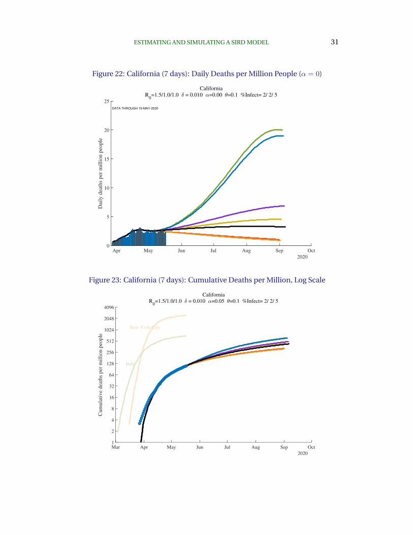
To see how this affects the results, consider Figure 22, which is based on the same


Figure 21: California (7 days): Daily Deaths per Million People

Apr May Jun Jul Aug Sep Oct

2020

0

1

2

3

4

5

6D

aily

dea

ths

per

mil

lio

n p

eop

le

California

R0=1.5/1.0/1.0 = 0.010 =0.05 =0.1 %Infect= 2/ 2/ 5


estimation for the past but assumes no feedback between behavior and daily

deaths, i.e. by setting α = 0. In this case, the swings in daily deaths are must

greater with deaths peaking above 20 per day rather than around 5 per day across

the different estimates. The key lesson here is that feedback matters tremen-

dously for future outcomes.

Returning to the baseline case of α = 0.05, Figure 23 shows the cumulative num-

ber of deaths in California going forward. By July, simulation results suggest any-

where from 200 to 300 deaths per million. This compares to a current stock of

deaths of around 100 per million.

United Kingdom. A similar illustration of this uncertainty is present in the graphs

for the United Kingdom. Figure 24 shows the changing futures as different death

numbers come in. R0 is estimated to have fallen from 2.4 at the start of the

pandemic to 1.1 today. The percent ever infected in the U.K. is estimated to be

8 percent as of early May.

The cumulative forecast is then shown in Figure 25. The number of predicted


Figure 22: California (7 days): Daily Deaths per Million People (α = 0)


2020

0

5

10

15

20

25D

aily

dea

ths

per

mil

lio

n p

eop

le

California

R0=1.5/1.0/1.0 = 0.010 =0.00 =0.1 %Infect= 2/ 2/ 5


Figure 23: California (7 days): Cumulative Deaths per Million, Log Scale

Mar Apr May Jun Jul Aug Sep Oct

2020

1

2

4

8

16

32

64

128

256

512

1024

2048

4096

Cum

ula

tive

dea

ths

per

mil

lion p

eople

California

R0=1.5/1.0/1.0 = 0.010 =0.05 =0.1 %Infect= 2/ 2/ 5

New York City

Italy


Figure 24: United Kingdom (7 days): Daily Deaths per Million People


2020

0

5

10

15

20

25D

aily

dea

ths

per

mil

lio

n p

eop

le

United Kingdom

R0=2.4/1.1/1.2 = 0.010 =0.05 =0.1 %Infect= 8/10/14


Figure 25: United Kingdom (7 days): Cumulative Deaths per Million, Log Scale


2020

1

2

4

8

16

32

64

128

256

512

1024

2048

4096

Cum

ula

tive

dea

ths

per

mil

lion p

eople

United Kingdom

R0=2.4/1.1/1.2 = 0.010 =0.05 =0.1 %Infect= 8/10/14

New York City

Italy

deaths is high, 850 per million — very similar to Italy.


Figure 26: United States (7 days): Daily Deaths per Million People


2020

0

1

2

3

4

5

6

7

8

9

10D

aily

dea

ths

per

mil

lio

n p

eop

le

United States

R0=2.0/1.0/1.1 = 0.010 =0.05 =0.1 %Infect= 5/ 6/ 8


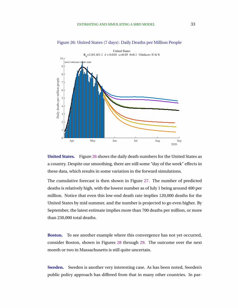
United States. Figure 26 shows the daily death numbers for the United States as

a country. Despite our smoothing, there are still some “day of the week” effects in

these data, which results in some variation in the forward simulations.

The cumulative forecast is then shown in Figure 27. The number of predicted

deaths is relatively high, with the lowest number as of July 1 being around 400 per

million. Notice that even this low-end death rate implies 120,000 deaths for the

United States by mid summer, and the number is projected to go even higher. By

September, the latest estimate implies more than 700 deaths per million, or more

than 230,000 total deaths.

Boston. To see another example where this convergence has not yet occurred,

consider Boston, shown in Figures 28 through 29. The outcome over the next

month or two in Massachusetts is still quite uncertain.

Sweden. Sweden is another very interesting case. As has been noted, Sweden’s

public policy approach has differed from that in many other countries. In par-


Figure 27: United States (7 days): Cumulative Deaths per Million, Log Scale


2020

1

2

4

8

16

32

64

128

256

512

1024

2048

4096

Cum

ula

tive

dea

ths

per

mil

lion p

eople

United States

R0=2.0/1.0/1.1 = 0.010 =0.05 =0.1 %Infect= 5/ 6/ 8

New York City

Italy

Figure 28: Boston (7 days): Daily Deaths per Million People


2020

0

10

20

30

40

50

60

70

Dai

ly d

eath

s p

er m

illi

on

peo

ple

Boston+Middlesex

R0=2.1/1.2/1.5 = 0.010 =0.05 =0.1 %Infect=15/20/32



ticular, one stylized view is that Sweden is trying to split its population into two

groups based on their different propensities to die if infected. A “high death rate”

group, for example the elderly and younger people who might be particularly

susceptible because of existing medical problems, could be encouraged to stay

home. The remaining “low death rate” group could be allowed to work, go to

school, and more generally remain involved in society. In this way, herd immunity

could potentially be achieved with a limited number of deaths. At this point, the

high risk group could be allowed to gradually reintegrate, possibly with masks and

other social distancing protocols in place.

Figures 30 and 31 show the results so far in Sweden. Two things stand out. First,

the percent of the overall population estimated to be infected is relatively low,

at 6 percent. This low number assumes a common death rate of 1.0%, but later

on in the paper in Table 2, we show that even with a death rate of 0.5%, only 12

percent of Sweden’s population is estimated to be infected. Second, the number

of cumulative deaths is not especially low, having already reached more than

480 deaths per million people and projected to go even higher. This of course

does not mean that the stylized policy presented in the previous paragraph is not

worth trying and potentially valuable. In fact, a model of this kind of possibility is

studied by Acemoglu, Chernozhukov, Werning and Whinston (2020) and policies

that exploit heterogeneity in the extent to which different populations may die

from the virus can lead to better outcomes in their setup. Perhaps Sweden did

not succeed in implementing such a policy or perhaps it doesn’t work after all for

some reason. More work will be needed on this question.

Other countries. The appendix and the dashboardcontain additional graphs for

other countries and regions. The patterns, uncertainties, and biases we have

highlighted above are apparent in these graphs as well. These graphs will be

updated frequently.



Figure 29: Boston (7 days): Cumulative Deaths per Million, Log Scale

Mar Apr May Jun Jul Aug Sep Oct

2020

1

2

4

8

16

32

64

128

256

512

1024

2048

4096

Cum

ula

tive

dea

ths

per

mil

lion p

eople

Boston+Middlesex

R0=2.1/1.2/1.5 = 0.010 =0.05 =0.1 %Infect=15/20/32

New York City

Italy

Figure 30: Sweden (7 days): Daily Deaths per Million People


2020

0

2

4

6

8

10

12

14

16

18

Dai

ly d

eath

s p

er m

illi

on

peo

ple

Sweden

R0=2.1/1.0/1.1 = 0.010 =0.05 =0.1 %Infect= 6/ 8/12



6. Problems with Geographic Aggregation

A point that is important to appreciate is that aggregating up from the city or

county to the state and to the national level can be misleading. SIRD is a nonlinear

model, so the results at the state level are not the same as the average of the results

at the county level.

This point is easy to illustrate using data from New York. We report results for sev-

eral different geographic regions. “New York City (plus)” includes New York City

plus the four surrounding counties of Nassau, Rockland, Suffolk, and Westchester,

with a total population of about 12 million. New York state is self explanatory

and has a population of about 20 million. And “New York excluding NYC” is the

difference between these other two: New York state excluding the NYC (plus) area,

with a population of about 8 million.

Now compare the results for these three regions, shown in Figures 32 through 34.

The results in New York state as a whole are driven entirely by New York City. For

example, imagine (counterfactually) that there were no deaths outside of New

York City. In this hypothetical case, deaths per million for New York state would

look exactly like deaths per million for New York City, except scaled down by a

factor of 12/20. Because of the lower deaths per million, the model would behave

slightly differently — New York state would be slower to achieve herd immunity

for example. And yet New York outside of New York City could look very different.

In fact, as the deaths in New York City decline, a potential rise in deaths outside of

New York City could cause the state death numbers to exhibit a flattening or even

a second peak.

Another version of this same kind of geographic aggregation bias seems likely to

occur for the United States itself (look back at Figure 26. To see this, imagine 50

states that sequentially pass through the peak of daily deaths. The U.S. national

number can be driven by New York (City!) for the first several weeks, then by

New Jersey and Michigan, and then by Massachusetts and Pennsylvania. The U.S.

graph may show a rise and then a very flat profile of deaths that persists for a

long time before declining, as new regions within the country suffer through their

peaks sequentially.


Figure 31: Sweden (7 days): Cumulative Deaths per Million, Log Scale


2020

1

2

4

8

16

32

64

128

256

512

1024

2048

4096

Cum

ula

tive

dea

ths

per

mil

lion p

eople

Sweden

R0=2.1/1.0/1.1 = 0.010 =0.05 =0.1 %Infect= 6/ 8/12

New York City

Italy

Figure 32: New York City (plus): Daily Deaths per Million People


2020

0

10

20

30

40

50

60

70

80

Dai

ly d

eath

s p

er m

illi

on

peo

ple


R0=2.6/0.5/0.9 = 0.010 =0.05 =0.1 %Infect=22/23/23



Figure 33: New York State: Daily Deaths per Million People


2020

0

10

20

30

40

50

60

Dai

ly d

eath

s p

er m

illi

on

peo

ple

New York

R0=2.6/0.9/1.2 = 0.010 =0.05 =0.1 %Infect=16/17/18


Figure 34: New York excluding NYC: Daily Deaths per Million People


2020

0

2

4

6

8

10

12

Dai

ly d

eath

s p

er m

illi

on

peo

ple

New York excluding NYC

R0=2.0/1.0/1.1 = 0.010 =0.05 =0.1 %Infect= 4/ 6/12



7. Herd Immunity and Re-Opening the Economy

An important question at this stage of the pandemic is how we go about re-opening

the economy. The estimation we’ve conducted has something helpful to con-

tribute on this point.

First, Table 2 reports the estimated fraction of the population that has ever been

infected as of May 9 for different countries and regions. Values for three different

values of δ are also reported, with the baseline case of δ = 1.0% in the center

column. Two key things stand out in the table. First, consider the baseline. As

we discussed above, we estimate that 26% of New Yorker City have ever been

infected.

In contrast, only 4 percent of people in New York state outside of New York City

and only 2 percent of Californians have ever been infected. There is enormous

heterogeneity in ever-infected rates. Where do these numbers come from? In our

model, the fraction δ of those infected eventually die, with the timing determined

by γ and θ, but essentially suggesting that deaths today reflect infections from 15

days earlier. With an assumed death rate of δ = 1.0%, for each death, there are

approximately 100 other people who have been infected. The large differences

in the number of deaths per million in New York versus California then translate

into these differences in infection rates. Interestingly, rates in Norway and South

Korea are similarly very low, while ever-infected rates in Italy, Spain, and France

are estimated to be around 6 to 8 percent.

The second point is that these numbers are — in an obvious way — very sensitive

to the assumed value of δ. If you double the death rate, you (roughly) halve the

ever-infected rate. If you halve the death rate, you (roughly) double the infected

rate. And as we discuss in more detail next, in thinking about herd immunity

and re-opening the economy, knowing the fraction ever-infected is crucial, at

least under the important assumption that antibodies give rise to immunity for

an extended period of time.

Notice that there is an important complementarity here. We would like the death

rate to be low, not just because it means that fewer people die, but also because

it means that lots of people will already have been infected. For example, if the


Table 2: Why Random Testing Would Be So Valuable

— Percent Ever Infected (today) —

δ = 0.5% δ = 1.0% δ = 1.2%

New York City (only) 51 26 22

New York City (plus) 44 22 19

Lombardy, Italy 43 22 19

New York 31 16 13

Madrid, Spain 36 18 15

Detroit 36 18 15

New Jersey 37 19 16

Stockholm, Sweden 36 18 15

Connecticut 33 17 14

Boston+Middlesex 29 15 12

Massachusetts 29 15 12

Paris, France 21 11 9

Philadelphia 23 12 10

Michigan 18 9 8

Spain 17 8 7

Chicago 21 11 9

District of Columbia 20 10 8

Italy 15 8 7

United Kingdom 16 8 7

France 13 6 5

Illinois 13 7 6

Sweden 12 6 5

Pennsylvania 12 6 5

United States 9 5 4

New York excluding NYC 8 4 3

Miami 7 3 3

U.S. excluding NYC 7 4 3

Ecuador 6 3 3

Los Angeles 5 3 2

Minnesota 5 3 2

Atlanta 5 3 2

Iowa 6 3 2

Florida 3 2 1

Germany 3 1 1

California 3 2 1

Brazil 4 2 2

Mexico 2 1 1

Norway 1 1 0


true death rate is 5 in 1000 rather than 10 in 1000, it means that 51 percent of

New Yorkers have already been infected and the herd immunity effects would be

very strong. In this sense, the finding that only 21 percent of New York City as

ever infected as of April 1 was doubly bad news: it pushes up the death rate and

means we are far from herd immunity, even in the place with the largest number

of infections.

As Atkeson (2020), Stock (2020), and others have emphasized, random testing

would be extremely helpful in identifying which of these cases is relevant. More-

over, the table suggests that if we are going to do 1000 random tests, you would

much rather do them in New York City than in California. So few people are

likely infected in California that it would be very hard to distinguish statistically

between the different death rates, whereas even 1000 random tests would be very

informative in New York City.

7.1 How far can we relax social distancing?

This brings us to the next reason why knowing the percent ever infected would be

so useful. The complement of this number is the percent of the population that

is still susceptible to the virus. Call this fraction s(t) ≡ S(t)/N (or better might be

S(t)/(N −D(t)) but D(t) is so low that it makes no difference).10

Recall from the basic SIR model that the virus will die out as long as

R0(t)s(t) < 1

That is, if R0t ≡ βt/γ is smaller than 1/s(t). The term s(t) is the herd immunity

term. The fewer people who are susceptible and the more people who are recov-

ered and hence immune, the less our random interactions result in infections. In

particular, we can relax social distancing — increase βt and R0t — to the critical

value such that R0ts(t) is just below one. That would mean that today’s infected

people infect fewer than one person on average, so the herd immunity keeps the

virus from re-surging.

10Notice, however, that our very stylized SIRD model is silent about how you map concrete policydecisions (i.e., should we or not open non-essential businesses) into changes in R0t.


Table 3: Using Percent Susceptible to Estimate Herd Immunity, δ = 1.0%

Percent R0(t+30) PercentSusceptible with no way back

R0 R0t t+30 outbreak to normal

New York City (only) 2.7 0.8 73.5 1.4 30.3

New York City (plus) 2.6 0.4 77.5 1.3 41.5

Lombardy, Italy 2.5 0.9 77.5 1.3 23.4

New York 2.6 0.7 83.8 1.2 26.4

Madrid, Spain 2.6 0.2 81.5 1.2 43.2

Detroit 2.4 0.5 81.6 1.2 37.6

New Jersey 2.6 1.1 78.3 1.3 11.4

Stockholm, Sweden 2.6 1.2 78.3 1.3 7.2

Boston+Middlesex 2.1 0.7 84.9 1.2 32.9

Massachusetts 2.1 1.0 83.3 1.2 21.3

Paris, France 2.4 0.2 89.4 1.1 42.0

Philadelphia 2.5 0.9 87.2 1.1 17.0

Michigan 2.4 0.7 90.6 1.1 25.0

Spain 2.4 0.5 91.5 1.1 29.8

Chicago 2.2 0.9 87.0 1.1 18.0

District of Columbia 2.0 0.9 87.9 1.1 19.0

Italy 2.2 1.0 91.5 1.1 6.8

United Kingdom 2.4 1.0 91.0 1.1 10.0

France 2.2 1.1 91.9 1.1 -6.0

Illinois 2.0 0.9 91.2 1.1 15.3

Sweden 2.1 0.9 92.7 1.1 15.2

Pennsylvania 2.1 0.8 93.0 1.1 19.5

United States 2.0 0.9 94.7 1.1 13.1

New York excluding NYC 2.0 1.1 92.8 1.1 -2.3

Miami 1.8 0.7 96.3 1.0 31.0

U.S. excluding NYC 1.8 0.9 95.6 1.0 11.8

Ecuador 1.5 0.8 95.7 1.0 30.8

Los Angeles 1.6 1.0 96.2 1.0 5.4

Minnesota 1.5 0.8 96.7 1.0 28.7

Atlanta 1.8 1.5 86.2 1.2 -84.9

Iowa 1.4 0.9 96.1 1.0 27.2

Washington 1.6 0.3 98.0 1.0 56.3

Florida 1.6 0.9 98.0 1.0 15.3

Germany 1.7 0.2 98.6 1.0 55.8

California 1.5 1.0 97.5 1.0 -3.4

Brazil 1.3 1.1 95.0 1.1 -54.7

SF Bay Area 1.3 1.0 98.8 1.0 10.3

Mexico 1.3 1.1 97.3 1.0 -45.8

Norway 1.6 0.2 99.4 1.0 58.9


Table 3 shows these calculations for one month from now (t+ 30) given the base-

line estimates from the model. For example, from the middle column, it is esti-

mated that in one month’s time, 78 percent of New York City (plus surrounding

counties) will still be susceptible. This means we could relax social distancing

to the point where R0 would rise to 1/0.78 = 1.3. This compares to the current

estimate for New York City of 0.4 and the initial estimate of 2.6. In other words, a

month from now, in this simulation (which may not adequately capture the real

world!), New York City could move 41% ([1.3-0.4]/[2.6-0.4]) of the way back to

normal and see no re-surgence of the virus.

The rest of the state of New York, in contrast, is estimated to still have 93% of

the population susceptible a month from now. So outside of the city, New York

needs to maintain its R0 at 1.1 — also its current level — to keep the virus from

spreading. New York City and the rest of New York state need different policies

if the fraction of the population that remains susceptible is as different as these

estimates imply.

Places with current values of R0 < 1 can relax somewhat and still keep the virus

in check. But the basic news from this table is that with a death rate of 1%, there

is very little herd immunity that has been accumulated and our scope for relaxing

social distancing is limited.11

On the other hand, if somehow this 1% death rate is overstated and the true death

rate is only 0.5%, the picture changes. The herd immunity effects for this case are

shown in Table 4. In this case, the greater New York City area has only about 56%

of its population susceptible because ever-infected rates are much higher. New

York City could move 57 percent of the way back to normal, raising R0 to 1.8, and

still not see a resurgence of the virus. Other places would also have more scope to

relax social distancing, at least somewhat.

This is why random testing in several places with a relatively high deaths per

million is so important: it will help us learn whether the numbers in Table 3 or 4

are more relevant.

11Notice, also, that these computations assume that individuals stay within their territories, and do notmove among them, mixing infection rates across areas.


Table 4: Herd Immunity with a Much Lower Death Rate, δ = 0.5%

Percent R0(t+30) PercentSusceptible with no way back

R0 R0t t+30 outbreak to normal

New York City (only) 2.7 1.6 46.6 2.1 51.1

New York City (plus) 2.6 0.7 56.1 1.8 56.6

Lombardy, Italy 2.5 1.5 54.4 1.8 30.6

New York 2.6 1.0 67.5 1.5 28.1

Madrid, Spain 2.6 0.3 64.1 1.6 55.9

Detroit 2.4 1.0 63.5 1.6 41.3

New Jersey 2.6 1.9 49.1 2.0 20.1

Stockholm, Sweden 2.6 1.8 52.1 1.9 11.6

Boston+Middlesex 2.1 1.4 61.8 1.6 33.7

Massachusetts 2.1 1.5 58.9 1.7 37.2

Paris, France 2.4 0.3 79.3 1.3 46.5

Philadelphia 2.5 1.3 66.9 1.5 13.2

Michigan 2.4 0.9 80.8 1.2 22.1

Spain 2.4 0.6 83.3 1.2 31.5

Chicago 2.2 1.1 71.3 1.4 30.1

District of Columbia 2.0 1.2 72.0 1.4 26.7

Italy 2.2 1.2 82.7 1.2 4.6

United Kingdom 2.4 1.2 80.8 1.2 7.2

France 2.2 1.2 84.3 1.2 -5.7

Illinois 2.0 1.0 81.4 1.2 21.7

Sweden 2.1 1.0 84.6 1.2 16.1

Pennsylvania 2.1 1.1 83.4 1.2 12.5

United States 2.0 1.0 89.0 1.1 11.8

New York excluding NYC 2.0 1.1 87.7 1.1 6.7

Miami 1.8 0.8 92.4 1.1 29.8

U.S. excluding NYC 1.8 1.0 90.8 1.1 11.2

Ecuador 1.5 0.9 91.2 1.1 36.1

Los Angeles 1.6 1.0 92.4 1.1 6.7

Minnesota 1.5 0.9 93.1 1.1 28.5

Atlanta 1.8 1.4 87.5 1.1 -77.7

Iowa 1.4 0.9 92.2 1.1 33.9

Washington 1.6 0.3 96.0 1.0 57.4

Florida 1.6 1.0 96.0 1.0 14.1

Germany 1.7 0.2 97.3 1.0 56.5

California 1.5 1.0 95.3 1.0 0.7

Brazil 1.3 1.1 92.5 1.1 4.4

SF Bay Area 1.3 1.0 97.7 1.0 11.0

Mexico 1.3 1.1 95.7 1.0 -17.4

Norway 1.6 0.2 98.9 1.0 58.9


7.2 What happens if we re-open the economy?

We now show simulations of what happens if we relax social distancing and in-

crease the value of R0 (i.e., β). The next set of graphs assume that more generous

policies are adopted one month from “today,” (which varies by country), i.e., on

something like June 9. Four simulation results are shown in each graph:

– The black line assumes the R0 from early May remains in place forever.

– The red line assumes that R0 rises slightly to 1/s(t), i.e., to the level that

would just keep the virus from exploding based on the current number of

susceptible people (as of early May again).

– The green line assumes we increase R0 by 25% back toward normal, i.e., by

25% of the way back from the May 9 estimate toward the initial level of R0.

– Finally, the purple line is similar except we increase R0 by to 50% of the way

back to normal.

For these simulations, we assume that the new value of R0 remains in place for-

ever. In practice, of course, one imagines that if deaths started to rise significantly,

mitigation policies would be re-adopted.

For comparison, these graphs also show — in the light brown bars — the daily

deaths per million in New York City. This is helpful in judging how severe a resur-

gence of the virus might be in different scenarios. For example, if Spain were

to move 50 percent of the way back to normal (the purple line), the predicted

resurgence would be much more severe than New York City experienced. Even

with a 25 percent return to normal, the rise in deaths would be comparable to

New York City, albeit with a lag into the late summer.

Finally, note that the SIRD model has “momentum.” Even if an area has reached

the threshold R0(t)s(t) < 1, we will continue accumulating infections and deaths

before the epidemic dies out fully. The number of these “overshoot” infections

and deaths will depend on the number of infectious individuals when we reach

R0(t)s(t) < 1. This observation is not a minor point. In a conventional SIRD

model where R0(t) gives you herd immunity at 60% of the population, if we reach

s(t) = 0.4 too fast, we can end up with over 90% of the population ever infected,


Figure 35: Spain: Re-opening

that is, with an extra 30% of infections over those required to achieve herd immu-

nity.

This means that we want to reach the threshold R0(t)s(t) < 1 or stay around it

with very few infectious individuals to minimize “overshoot” infections. While

setting up and solving an optimal control problem of the COVID-19 epidemic in

the tradition of Morton and Wickwire (1974) to get to such an objective is beyond

the scope of our paper, our empirical results can help to calibrate re-opening

scenarios such as those quantitatively explored in Baqaee, Farhi, Mina and Stock

(2020).


Figure 36: Italy: Re-opening

Figure 37: New York City: Re-opening


Figure 38: New York excluding NYC: Re-opening

Figure 39: Los Angeles: Re-opening


Figure 40: Stockholm, Sweden: Re-opening

Figure 41: Chicago: Re-opening


Figure 42: Massachusetts: Re-opening


8. Conclusions

The first thing to (re)emphasize about these simulations is that we are economists,

not epidemiologists. These are speculations based on estimation and simulation

of a relatively simple and standard model. We find them helpful for thinking

about the dynamics of the pandemic, but great care should be taking in using

these numbers to inform any policy discussion.

Relative to the standard SIRD model in the literature, we include a time-varying

β, and therefore a time-varying R0. We invert the SIRD model to back out the

daily values of R0t that fit the death data. We see this as important for capturing

behavioral changes by individuals in response to the pandemic as well as policy

changes related to social distancing. We also include an additional “recovering”

state that is consistent with the medical evidence that cases seem to be infec-

tious for four to five days while taking a total of several weeks or more to resolve.

These changes connect the model better to the epidemiology of the virus and

are important in improving the model’s ability to fit the data. Finally, we follow

Cochrane (2020) and include feedback between R0t and daily deaths in modeling

the future of the epidemic. We hope that our empirical estimates will prove useful

to others in thinking about the possible path that COVID-19 may take as different

locations open up in different ways, and we will continue to update our results on

our dashboard.

References

Acemoglu, Daron, Victor Chernozhukov, Ivan Werning, and Michael D. Whinston, “A

Multi-Risk SIR Model with Optimally Targeted Lockdown,” Technical Report, MIT 2020.

Alvarez, Fernando E., David Argente, and Francesco Lippi, “A Simple Planning Problem

for COVID-19 Lockdown,” Working Paper 26981, National Bureau of Economic Re-

search April 2020.

Atkeson, Andrew, “How Deadly Is COVID-19? Understanding The Difficulties With

Estimation Of Its Fatality Rate,” Working Paper 26965, National Bureau of Economic

Research April 2020.



Avery, Christopher, William Bossert, Adam Clark, Glenn Ellison, and Sara Fisher Ellison,

“Policy Implications of Models of the Spread of Coronavirus: Perspectives and Oppor-

tunities for Economists,” Working Paper 27007, National Bureau of Economic Research

April 2020.

Baqaee, David, Emmanuel Farhi, Michael J Mina, and James H Stock, “Reopening

Scenarios,” Working Paper 27244, National Bureau of Economic Research May 2020.

Bar-On, Yinon M., Avi Flamholz, Rob Phillips, and Ron Milo, “SARS-CoV-2 (COVID-19) by

the numbers,” Technical Report March 2020.

Bendavid, Eran, Bianca Mulaney, Neeraj Sood, Soleil Shah, Emilia Ling, Rebecca Bromley-

Dulfano, Cara Lai, Zoe Weissberg, Rodrigo Saavedra, James Tedrow, Dona Tversky,

Andrew Bogan, Thomas Kupiec, Daniel Eichner, Ribhav Gupta, John Ioannidis, and Jay

Bhattacharya, “COVID-19 Antibody Seroprevalence in Santa Clara County, California,”

medRxiv, 2020.

Berger, David W, Kyle F Herkenhoff, and Simon Mongey, “An SEIR Infectious Disease

Model with Testing and Conditional Quarantine,” Working Paper 26901, National

Bureau of Economic Research March 2020.

Bethune, Zachary A and Anton Korinek, “Covid-19 Infection Externalities: Trading Off

Lives vs. Livelihoods,” Technical Report, National Bureau of Economic Research 2020.

Bodenstein, Martin, Giancarlo Corsetti, and Luca Guerrieri, “Social Distancing and

Supply Disruptions in a Pandemic,” Technical Report 2020-031 04 2020.

Brauer, F., C. Castillo-Chavez, and Z. Feng, Mathematical Models in Epidemiology,

Springer New York, 2019.

Chari, Varadarajan V, Rishabh Kirpalani, and Christopher Phelan, “The Hammer and the

Scalpel: On the Economics of Indiscriminate versus Targeted Isolation Policies during

Pandemics,” Working Paper 27232, National Bureau of Economic Research May 2020.

Chowell, Gerardo, Cecile Viboud, Lone Simonsen, and Seyed M. Moghadas, “Charac-

terizing the Reproduction Number of Epidemics with Early Subexponential Growth

Dynamics,” Journal of The Royal Society Interface, 2016, 13 (123), 20160659.

Cochrane, John, “An SIR Model with Behavior,” May 2020. The Grumpy Economist blog,

https://johnhcochrane.blogspot.com/.

Eichenbaum, Martin S, Sergio Rebelo, and Mathias Trabandt, “The Macroeconomics of

Epidemics,” Working Paper 26882, National Bureau of Economic Research March 2020.

https://johnhcochrane.blogspot.com/


Farboodi, Maryam, Gregor Jarosch, and Robert Shimer, “Internal and External Effects

of Social Distancing in a Pandemic,” Technical Report 2020-47 2020. University of

Chicago, Becker Friedman Institute for Economics Working Paper.

Garriga, Carlos, Rody Manuelli, and Siddhartha Sanghi, “Optimal Management of an

Epidemic: An Application to COVID-19. A Progress Report,” Technical Report April

2020. Federal Reserve Bank of St. Louis manuscript.

Hethcote, Herbert W., “The Mathematics of Infectious Diseases,” SIAM Review, 2000, 42

(4), 599–653.

Hornstein, Andreas, “Social Distancing, Quarantine, Contact Tracing, and Testing: Im-

plications of an Augmented SEIR-Mode,” Technical Report, Federal Reserve Bank of

Richmond 2020.

Hortasu, Ali, Jiarui Liu, and Timothy Schwieg, “Estimating the Fraction of Unreported In-

fections in Epidemics with a Known Epicenter: an Application to COVID-19,” Working

Paper 27028, National Bureau of Economic Research April 2020.

Hurwicz, Leonid, “On the Structural Form of Interdependent Systems,” in Ernest Nagel,

Patrick Suppes, and Alfred Tarski, eds., Logic, Methodology and Philosophy of Science,

Vol. 44 of Studies in Logic and the Foundations of Mathematics, Elsevier, 1962, pp. 232

– 239.

Imperial College COVID-19 Response Team, “Impact of non-pharmaceutical interven-

tions (NPIs) to reduce COVID19 mortality and healthcare demand,” Technical Report,

Imperial College 2020.

Johns Hopkins University CSSE, “2019 Novel Coronavirus COVID-19 (2019-nCoV) Data

Repository,” 2020. Center for Systems Science and Engineering.

Karin, Omer, Yinon M Bar-On, Tomer Milo, Itay Katzir, Avi Mayo, Yael Korem, Boaz

Dudovich, Eran Yashiv, Amos J Zehavi, Nadav Davidovich et al., “Adaptive cyclic

exit strategies from lockdown to suppress COVID-19 and allow economic activity,”

medRxiv, 2020.

Katz, Josh and Margot Sanger-Katz, “N.Y.C. Deaths Reach 6 Times the Normal Level, Far

More Than Coronavirus Count Suggests,” The New York Times, April 2020.

Kermack, William Ogilvy and A. G. McKendrick, “A contribution to the mathematical

theory of epidemics, part I,” Proceedings of the Royal Society of London. Series A, 1927,

115 (772), 700–721.


and , “Contributions to the mathematical theory of epidemics. II – The problem of

endemicity,” Proceedings of the Royal Society of London. Series A, 1932, 138 (834), 55–83.

Korolev, Ivan, “Identification and Estimation of the SEIRD Epidemic Model for COVID-

19,” Technical Report, Binghamton University 2020.

, “What Does the Case Fatality Ratio Really Measure?,” Technical Report, Binghamton

University 2020.

Kucinskas, Simas, “Tracking R of COVID-19,” Available at SSRN 3581633, 2020.

Linton, Oliver, “When will the Covid-19 pandemic peak?,” Technical Report, University of

Cambridge 2020.

Liu, Laura, Hyungsik Roger Moon, and Frank Schorfheide, “Panel Forecasts of Country-

Level Covid-19 Infections,” Working Paper 27248, National Bureau of Economic Re-

search May 2020.

Morton, R. and K. H. Wickwire, “On the Optimal Control of a Deterministic Epidemic,”

Advances in Applied Probability, 1974, 6 (4), 622–635.

New York Department of Health, “The NYSDOH Wadsworth Center’s Assay for SARS-CoV-

2 IgG,” Technical Report April 2020.

Sanche, S., Y.T. Lin, C. Xu, E. Romero-Severson, N. Hengartner, and R. Ke, “High

contagiousness and rapid spread of severe acute respiratory syndrome coronavirus 2,”

Emerging Infectious Diseases, 2020, 26.

Stock, James H, “Data Gaps and the Policy Response to the Novel Coronavirus,” Working

Paper 26902, National Bureau of Economic Research March 2020.

The Economist, “Tracking covid-19 excess deaths across countries,” April 2020.

Toda, Alexis Akira, “Susceptible-Infected-Recovered (SIR) Dynamics of COVID-19 and

Economic Impact,” 2020. U.C.S.D. manuscript.

A. Graphs for Other Countries, States, and Cities

Graphs for many countries and regions are shown below. We report detailed and

extended results for even more countries, states, and cities on our web pages and

plan to update the dashboard frequently.

https://web.stanford.edu/~chadj/Covid/Dashboard.html


Figure 43: France (7 days): Daily Deaths per Million People


2020

0

5

10

15

20

25

Dai

ly d

eath

s p

er m

illi

on

peo

ple

France

R0=2.2/1.2/1.1 = 0.010 =0.05 =0.1 %Infect= 6/ 8/12


Figure 44: Philadelphia (7 days): Daily Deaths per Million People


2020

0

5

10

15

20

25

30

35

40

Dai

ly d

eath

s p

er m

illi

on

peo

ple

Philadelphia

R0=2.5/1.2/1.4 = 0.010 =0.05 =0.1 %Infect=12/18/31



Figure 45: Washington (7 days): Daily Deaths per Million People


2020

0

1

2

3

4

5

6

7

8

9

Dai

ly d

eath

s p

er m

illi

on

peo

ple

Washington

R0=1.6/0.3/0.4 = 0.010 =0.05 =0.1 %Infect= 2/ 2/ 2


Figure 46: Louisiana (7 days): Daily Deaths per Million People


2020

0

5

10

15

20

25

Dai

ly d

eath

s p

er m

illi

on

peo

ple

Louisiana

R0=2.2/1.0/1.1 = 0.010 =0.05 =0.1 %Infect= 8/10/13



Figure 47: Florida (7 days): Daily Deaths per Million People


2020

0

0.5

1

1.5

2

2.5

3

3.5

4

Dai

ly d

eath

s p

er m

illi

on

peo

ple

Florida

R0=1.6/0.9/1.0 = 0.010 =0.05 =0.1 %Infect= 2/ 2/ 3


Figure 48: Connecticut (7 days): Daily Deaths per Million People


2020

0

5

10

15

20

25

30

35

40

45

50

Dai

ly d

eath

s p

er m

illi

on

peo

ple

Connecticut

R0=2.5/1.5/1.7 = 0.010 =0.05 =0.1 %Infect=17/25/43


Documents

Estimating andSimulating a SIRDModel ofCOVID ...web.stanford.edu/~chadj/sird-paper.pdfdemographic and selection-into-disease mechanism, which are themselves partly the product of endogenous