Essays on Dynamic Marketing Intercommunications

by

Kee Yeun Lee

A dissertation submitted in partial fulfillmentof the requirements for the degree of

Doctor of Philosophy(Business Administration)

in The University of Michigan2013

Doctoral Committee:

Professor Fred M. Feinberg, ChairAssistant Professor Elizabeth E. BruchProfessor Richard D. GonzalezProfessor Peter J. Lenk

c© Kee Yeun Lee 2013

All Rights Reserved

To my parents -

Seung Hyun Lee and Young Nam Byun

ii

ACKNOWLEDGEMENTS

I would like to express my sincere gratitude to the members of my dissertation com-

mittee. First and foremost, I am deeply indebted to my advisor, Fred Feinberg, for his

guidance, infinite patience, and endless support. Whenever I felt I was failing or was in

need of desperate help, he has always been made himself available for me. His dedication

made it possible to complete my long journey to Ph.D. which once seemed to be almost

impossible. He deserves a title “The World’s Best Advisor” and I am deeply honored to

have him as my academic father. I am also deeply grateful to Elizabeth Bruch who gave

me enormous support for the second essay throughout the project. It has been a true joy for

me to work with you and I expect our future projects to be more enjoyable. I would also

like to thank the other dissertation committee members, Rich Gonzalez and Peter Lenk, for

their insightful feedback and advice.

I would like to extend my thanks to my friends and colleagues: Na Eun Cho, Yoon Sun

Han, Bo Kyung Kim, Gi Hyun Kim, Yun Jung Kim, Hyun Jee Kim, Na Na Lee, Jin Kyung

Na, Hee Mok Park, Jong Sang Park, and Sun Hyun Park. Thanks for being my family

during my graduate program in Ann Arbor.

Last and most importantly, I am deeply grateful to my family - my father, Seung Hyun

Lee, my mother, Young Nam Byun, and my sister, Jae Hwa Lee - for always being there

with their everlasting love and support. They have been always believing in me and en-

couraging me to complete the doctoral degree. Without their love and support, it would not

have been possible for me to finish this journey successfully. No words can express how

much I thank and love them.

iii

TABLE OF CONTENTS

DEDICATION . . . . . . . . . . . . . . . . . . . . . . . . . . . . . . . . . . . ii

ACKNOWLEDGEMENTS . . . . . . . . . . . . . . . . . . . . . . . . . . . . iii

LIST OF FIGURES . . . . . . . . . . . . . . . . . . . . . . . . . . . . . . . . vi

LIST OF TABLES . . . . . . . . . . . . . . . . . . . . . . . . . . . . . . . . . vii

ABSTRACT . . . . . . . . . . . . . . . . . . . . . . . . . . . . . . . . . . . . . viii

CHAPTER

I. INTRODUCTION . . . . . . . . . . . . . . . . . . . . . . . . . . . . . . 1

II. Modeling Scale Attraction Effects: An Application to Charitable Do-nations and Optimal Laddering . . . . . . . . . . . . . . . . . . . . . . 3

2.1 Abstract . . . . . . . . . . . . . . . . . . . . . . . . . . . . . . . 32.2 Introduction . . . . . . . . . . . . . . . . . . . . . . . . . . . . . 42.3 Literature Review . . . . . . . . . . . . . . . . . . . . . . . . . . 72.4 Data Description . . . . . . . . . . . . . . . . . . . . . . . . . . . 102.5 Model Development . . . . . . . . . . . . . . . . . . . . . . . . 13

2.5.1 Internal and External Reference Points . . . . . . . . . . 132.5.2 Modeling Scale Attraction Effects . . . . . . . . . . . . 142.5.3 General Model(Type 2 Tobit) . . . . . . . . . . . . . . . 222.5.4 Explanatory variables and Heterogeneity . . . . . . . . 23

2.6 Estimation . . . . . . . . . . . . . . . . . . . . . . . . . . . . . . 272.7 Results . . . . . . . . . . . . . . . . . . . . . . . . . . . . . . . . 29

2.7.1 Error Correlation in Selection and Amount equations . . 302.7.2 Selection: Seasonality . . . . . . . . . . . . . . . . . . 302.7.3 Level Dummies and Lagged Log-Amount . . . . . . . . 312.7.4 “Pulling Effects”: Gamma Kernel Parameters in Dona-

tion Amount . . . . . . . . . . . . . . . . . . . . . . . 32

iv

2.8 Model comparison . . . . . . . . . . . . . . . . . . . . . . . . . . 362.9 Illustrative Application: Effect of individually tailored appeals scales 412.10 Conclusion . . . . . . . . . . . . . . . . . . . . . . . . . . . . . . 442.11 Appendix . . . . . . . . . . . . . . . . . . . . . . . . . . . . . . . 47

III. Modeling Mate Choice Behavior: A Two-Stage Mate Choice Modelwith Potentially Non-Compensatory Decision Rules . . . . . . . . . . . 56

3.1 Abstract . . . . . . . . . . . . . . . . . . . . . . . . . . . . . . . 563.2 Introduction . . . . . . . . . . . . . . . . . . . . . . . . . . . . . 573.3 Model development . . . . . . . . . . . . . . . . . . . . . . . . . 59

3.3.1 Hypotheses on mate choice behavior . . . . . . . . . . . 603.3.2 Decision rules . . . . . . . . . . . . . . . . . . . . . . . 623.3.3 Utility functions . . . . . . . . . . . . . . . . . . . . . 653.3.4 Two-stage model of mate choice . . . . . . . . . . . . . 70

3.4 Estimation . . . . . . . . . . . . . . . . . . . . . . . . . . . . . . 733.4.1 ECM algorithm . . . . . . . . . . . . . . . . . . . . . . 733.4.2 Mixture of logits model with changepoints . . . . . . . 743.4.3 Parameter recovery . . . . . . . . . . . . . . . . . . . . 75

3.5 Empirical results . . . . . . . . . . . . . . . . . . . . . . . . . . . 783.5.1 Data description . . . . . . . . . . . . . . . . . . . . . 783.5.2 The Process of Finding a Mate Online . . . . . . . . . . 813.5.3 Estimation results . . . . . . . . . . . . . . . . . . . . . 83

3.6 Conclusion . . . . . . . . . . . . . . . . . . . . . . . . . . . . . . 933.7 Appendix . . . . . . . . . . . . . . . . . . . . . . . . . . . . . . . 96

IV. CONCLUSION . . . . . . . . . . . . . . . . . . . . . . . . . . . . . . . 111

BIBLIOGRAPHY . . . . . . . . . . . . . . . . . . . . . . . . . . . . . . . . . 113

v

LIST OF FIGURES

Figure

2.1 Examples of Appeals Scales used by Charities . . . . . . . . . . . . . . . 52.2 Compliance Degree Curves . . . . . . . . . . . . . . . . . . . . . . . . . 182.3 Pulling Amount Curves . . . . . . . . . . . . . . . . . . . . . . . . . . . 192.4 Pulling amounts owing to multiple scale (external reference) points . . . . 252.5 Distribution of Mean and SE of observed amounts for each donor . . . . . 262.6 Upward and downward compliance curves at gamma posterior mean . . . 312.7 Upward and downward pulling amount curves at gamma posterior mean . 322.8 Gamma parameters (up and down) for each donor . . . . . . . . . . . . . 332.9 Scale point with maximum upward pull . . . . . . . . . . . . . . . . . . 342.10 Maximum pulling up and down amounts for each donor . . . . . . . . . . 363.1 Decision rules for continuous (ordinal) attributes . . . . . . . . . . . . . 693.2 Decision rules for categorical attributes . . . . . . . . . . . . . . . . . . . 693.3 Diagram of Mate Choice Process . . . . . . . . . . . . . . . . . . . . . . 703.4 Browsing - Age difference for Male and Female users . . . . . . . . . . . 863.5 Writing - Age difference for Male users . . . . . . . . . . . . . . . . . . 913.6 Writing - Age difference for Female users . . . . . . . . . . . . . . . . . 913.7 Writing - Height difference for Male users . . . . . . . . . . . . . . . . . 923.8 Writing - Height difference for Female users . . . . . . . . . . . . . . . . 93

vi

LIST OF TABLES

Table

2.1 Appeals Scales used in the Field Experiment . . . . . . . . . . . . . . . . 112.2 Average Donation Amounts and Frequencies . . . . . . . . . . . . . . . . 122.3 Yield Rate and Average Amount of Observed Donations across Seasons . 132.4 Examples of Donation Histories for Several Randomly Selected Households 232.5 Mean and SE of observed amounts (FF) for each donor . . . . . . . . . . 242.6 Parameter Estimates for Full Model . . . . . . . . . . . . . . . . . . . . 292.7 In-sample fit of observed donation amounts . . . . . . . . . . . . . . . . 382.8 In-sample fit of observed donation amounts (Full model with IR-1) . . . . 392.9 Expected value of average donation amount in simulation . . . . . . . . . 433.1 Simulation results for a two component mixture of logits model . . . . . . 763.2 Simulation results for a three component mixture of logits model . . . . . 773.3 user registration information (continuous attributes) . . . . . . . . . . . . 793.4 user registration information (discrete attributes) . . . . . . . . . . . . . . 803.5 Activity data (male users) . . . . . . . . . . . . . . . . . . . . . . . . . . 823.6 Activity data (female users) . . . . . . . . . . . . . . . . . . . . . . . . . 833.7 Parameter estimates for Browsing behavior . . . . . . . . . . . . . . . . 853.8 Parameter estimates for Writing behavior . . . . . . . . . . . . . . . . . 873.9 Writing - Education level for Male users . . . . . . . . . . . . . . . . . . 883.10 Writing - Education level for Female users . . . . . . . . . . . . . . . . . 88

vii

ABSTRACT

The dissertation examines two distinct problems related to “marketing communication

dynamics”. The main goal of this line of research is to help firms provide individually

tailored marketing contents to their customers. In these two essays, I develop statistical

models to first understand customers’ responses, and then explore methods to optimize

firms’ reactions accordingly. Essay 1 examines “scale attraction effects” in a charitable

donation context, introducing novel constructs (“compliance degree”, “pulling amount”,

“accumulated pulling amount”) to describe attraction effects for multi-point appeals scales.

The proposed model jointly accounts for donation incidence and amount using a Tobit 2

formulation, and allows heterogeneity in seasonality and pulling effects. Results suggest

substantial scale attraction effects that vary across donors, stronger “pulling down” than

“pulling up”, and heterogeneous seasonal donation patterns. A significantly negative error

correlation between donation incidence and donation amount underscores the importance

of accounting for selectivity effects. The effects of individually tailoring appeals scales is

demonstrated through simulation.

Essay 2 investigates mate-seeking users’ decision rules in an online dating context. I

develop an empirical two-stage mate choice model that can accommodate compensatory

and non-compensatory decision rules in each of two stages: browsing and writing. A

mixture of logits model with changepoints allows for distinct decision rules across stages

and heterogeneity in rule use across site users. Most importantly, it allows us to identify

and compare attribute-level decision rules (“deal-breakers” and “deal-makers”) over the

two stages. Results suggest the existence of heterogeneity in decision rules across (1)

genders, (2) stages, and (3) site users. Additionally, it suggests the existence of potential

viii

deal-breakers/makers across both discrete and continuous attributes.

ix

CHAPTER I

INTRODUCTION

This dissertation develops models of dynamic intercommunication: between firms and

their customers and among customers themselves. In these essays, I am interested in not

only measuring customers’ responses to firms’ marketing communication actions (stimuli),

but also how firms can optimize such stimuli to individual customers in a dynamic man-

ner. This stream of research is particularly intriguing to me, as small changes in marketing

communications - such as scaling (1st essay), and matching algorithm (2nd essay) can ex-

ert great impact on customers’ behaviors by simply ”nudging” them appropriately. Such

nudging can help firms to maximize the efficiency of marketing communications, as well

help customers to find the products/services that best fit their needs. That is, without in-

vestments in costly new campaigns or infrastructure, firms can (algorithmically, optimally)

tune their personalized marketing intercommunications, over time.

The first, “Modeling Scale Attraction Effects: An Application to Charitable Donations

and Optimal Laddering” examines scale attraction effects when approaching individual po-

tential donors. Panel data from a unique 3.5 year quasi-experiment enables a joint account

of both whether a donation is made (incidence) and, if so, its size (amount). The model

incorporates heterogeneity across donors in scale attraction effects and donation patterns

(e.g., seasonality), and allows tests of distinct operationalizations of internal and external

reference price theories. Results suggest that scale points do exert substantial attraction ef-

1

fects; that these vary markedly across donors; that donors are more easily persuaded to give

less than more; and that seasonal donation patterns are pronounced. A significantly nega-

tive error correlation between (latent) donation propensity and (observed) donation amount

highlights the importance of accounting for selectivity effects. We illustrate the framework

with a speculative application to “laddering”: how much charities should increase amounts

subsequently requested of individual donors, based on their donation histories.

The second essay, “Modeling mate choice behavior: A two-stage mate choice model

with potentially non-compensatory decision rules” allows us to empirically evaluate al-

ternative decision rules used by individuals who interacted via an online dating service

provider in the US. The proposed model captures the intrinsically multistage behavior in-

volved in many online transactions, but in particular dating, where one decides which pro-

files to browse and then (stage 1), conditional on having browsed, whom to write to (stage

2), if anyone. Here, we account for these two distinct activities by modeling the binary

decisions (of browsing and writing). The model can accommodate compensatory and non-

compensatory decision rules in each stage; it allows decision rules to differ across stages;

different attributes can be modeled as having distinctly different utility ‘shapes’; and het-

erogeneity in rule use across site users provides interpretable profiles of different types of

mate-seeking behavior. Finally, and most importantly, we directly model the utility func-

tions of attributes to identify and compare attribute-level decision rules (“deal-breakers”

and “deal-makers”) over the two distinct stages. Based on the model and direct extensions

to other data settings, firms can offer more accurate, targeted search among potential dyads,

in online dating, social networks, and even among various users of online shopping sites.

2

CHAPTER II

Modeling Scale Attraction Effects: An Application to

Charitable Donations and Optimal Laddering

2.1 Abstract

Charities seeking donations usually employ an “appeals scale,” a set of specific suggested

amounts presented directly to potential donors. Choosing them well is crucial: if chari-

ties select overly high scale points, they risk their being ignored or even alienating donors

and receiving nothing, while overly low scale points may encourage donors to give less

than they’d have otherwise. Despite their widespread use, little is known about the degree

to which the points on such scales affect both whether a donation is made and, if so, its

size. Using panel data from a 3.5 year quasi-experiment, we develop a joint model ac-

counting for both donation incidence and amount. The model incorporates heterogeneity

across donors in both scale attraction effects and in donation patterns (e.g., seasonality),

and allows tests of distinct operationalizations of internal and external reference price the-

ories. Results suggest that scale points do exert substantial attraction effects; that these vary

markedly across donors; that donors are more easily persuaded to give less than more; and

that there are strong seasonal donation patterns in giving. A significantly negative corre-

lation between error terms in (latent) donation propensity and (observed) donation amount

highlights the importance of accounting for selectivity effects. We illustrate the framework

3

with a speculative application to “laddering”: how much charities should increase amounts

subsequently requested of individual donors, based on their donation histories.

2.2 Introduction

Solicitations for charitable donations are a part of everyday life, with requests being made

at physical locations (stores, workplaces), through the mail, various media (radio, televi-

sion), and increasingly via the Internet (e-mail, websites, social networks). The Center on

Philanthropy at Indiana University (2010) recently listed over 1.2 million charitable orga-

nizations in the United States alone, as of 2009.1 The total amount of giving in the US

has increased rapidly over the past decade, with $303B in 2009, an 80% inflation-adjusted

increase over 20 years earlier. These donations account for 2.1% of U.S. GDP, a quantity

ahead of all but 3 corporations in revenues and all in profits.

Private citizens have been generous to charities, even during the recent economic down-

turn, with 65% of US households donating per annum, $1,940 on average (including non-

donors). Household-level donation, $227.4B in 2009, accounts for 75% of the U.S. total,

followed by foundations ($38.4B; 13%), bequests ($23.8B; 8%), and corporations ($14.1B;

4%).

Potential donors are typically presented with an “appeals scale”, a list of suggested

amounts or scale points selected by fundraisers. Figure 2.1 presents three such scales, used

for recent funding drives by Wikipedia, the United Way, and the U. N. Foundation. Each

features the most common sort of appeals scale: a series of specific donation amounts,

along with an “open” category. The appeals scale serves several functions, but its main role

is to provide concrete anchors to help donors select an appropriate quantity; donors can,

of course, also choose to give nothing, or some amount not listed on the scale, including

amounts outside the range of listed values.

12009 is the last year for which comprehensive statistics are presently available, so it is adopted consis-tently for comparison purposes.

4

A. Wikipedia: wikipedia.org

B. United Way: liveunited.org

C. United Nations Foundation: unfoundation.org

Figure 2.1: Examples of Appeals Scales used by Charities

Holding aside questions involving the design of an entire scale, an immediate practical

concern for fundraisers is simply about how much to ask for: too little, and a donor may

be more likely to give, but to give less; too much, and a donor may fail to be influenced by

the request, or simply not donate at all. Charities wish to maximize donations, and so must

attempt to tailor their requests to avoid asking for inappropriate or suboptimal donation

amounts.

5

Despite their ubiquity in charitable requests and fundraising, there is neither theory

nor a body of empirical findings on whether and to what degree such requests, and the

scales comprising them, affect individual donor behavior. As a result, fundraisers have little

rigorous guidance in assessing and optimizing their appeal requests, instead falling back on

prior experience, coupled with summary metrics arising from trial and error (which, as we

shall see, can produce misleading or even null results). Part of the problem in providing

such guidance is the need for household-level, longitudinal data on both charitable requests

and outcomes - “whether” and “how much” - which charities typically possess, along with

a (suitably heterogeneous) statistical model for scale attraction effects, which they typically

do not.

Some of these issues have been addressed in prior literature, for example, Desmet &

Feinberg (2003) and De Bruyn & Prokopec (2011), each of whom examined scale effects

statistically via recourse to both internal (donors’ latent, planned amounts) and external

(how much one is asked for) reference points (Mayhew & Winer, 1992; Mazumdar & Pap-

atla, 2000). Although both detected scale-based effects, neither was able to incorporate het-

erogeneity (the basis of individually-tailored appeals), seasonal variation in giving (which

is pronounced in our empirical application), nor simultaneously account for whether and

how much to give, which can lead to selection biases (Van Diepen et al., 2009; Wachtel &

Otter, 2011). In this paper, we resolve these and several other issues via a novel model that

measures individual-level scale attraction effects. The model, which builds upon a clas-

sic Type 2 Tobit formulation, is calibrated on donation history panel data from a French

charity.

The remainder of the paper is organized as follows. We first provide a concise overview

of prior literature on scale attraction, donation behavior, reference effects, and related areas.

We then describe our empirical application, develop the model, and present both empirical

results and model comparisons. An illustrative simulation exercise examining the effect of

tailored appeals scales is followed by potential limitations and associated future research.

6

2.3 Literature Review

The contextual effects of scaling on responses have been intensively examined in social

psychology over the past two decades. Schwarz (1999)’s comprehensive review suggests

that features of research instruments - question wording, format, and scaling, among others

- can substantially affect respondents’ self-reported behaviors and attitudes. In particular,

response scales presented to respondents are far more than a simple “measurement device,”

but can work as reference frames that directly influence respondents’ judgments (Schwarz

et al., 1991).

Researchers working in the area of social norms have found them to systematically in-

fluence human behaviors. Individuals seek out social norms to better understand or more

effectively react to social situations they encounter, especially under high uncertainty (Cial-

dini & Goldstein, 2004). Fisher & Ackerman (1998) support this “normative” perspective

in their studies on volunteerism, and several studies have examined the effects of social

information on donation behavior specifically. It has long been observed that manipulat-

ing such information (i.e., what other donors gave) can strongly affect donation behaviors

(Reingen, 1982); Shang et al. (2008) and Shang & Croson (2009) found exactly this in a

field test for a national radio fundraising campaign. When other donors’ behavior is not

disclosed during a donation appeal (which is typical), respondents are more uncertain in

deciding a donation amount, so a given set of response alternatives - an appeals scale - can

provide contextually normative information via the location (i.e., distribution) of its scale

points (Schwarz et al., 1991).

Many studies have addressed charitable donations directly, and examined the role of

request size on donation behavior (amount and compliance) in laboratory and field data

(Doob & McLaughlin, 1989; Fraser et al., 1988; Schibrowsky & Peltier, 1995; Weyant &

Smith, 1987). Although contexts and methods vary across them, these studies largely con-

firm scale manipulation effects, yet differ as to whether they affect donation likelihood,

donation amount, or both (see De Bruyn & Prokopec, 2011, for review). These differences

7

may have originated from variations in compliance techniques, solicitation methods, and

the suggested donation amounts. One particularly compelling potential source for incon-

sistencies across prior studies is lack of an account of internal referents. In the words of

De Bruyn & Prokopec (2011), “... most fundraising research to date has overlooked the

crucial role of a donor’s internal reference point in moderating the impact of appeals scales

on behavior.” In marketing specifically, reference price theory has been a cornerstone of

consumer behavior research, and supported empirically in dozens of studies (Kalyanaram

& Winer, 1995, provide an extensive review).

We make especial use of one of the key findings from this literature: that two distinct

kinds of reference prices play a role in choice decisions. One is internal reference prices,

consumer-specific, memory-based amalgams of actual, recent (and “fair”) prices; the other

is external reference prices, present at the time of purchase. It is well-known that both

internal and external reference points play a role in consumer purchase decisions (May-

hew & Winer, 1992); in donation contexts, the former is characterized by what the donor

typically gives and/or plans to give, the latter what the donor is asked to. Specifically, the

internal referent is an unobservable construct that must be inferred from other observable

information (e.g., past donation behavior), while external referents are those presented at

the time of the request via the appeals scale. Prior work in donations was unable to employ

both referents, since individual-specific donation histories were lacking. Thus, researchers

were unable to avail of potential donors’ internal referents when designing scales for exper-

iments. This may have led to inconsistent scale manipulation results as reported by Weyant

& Smith (1987) vs. those of Doob & McLaughlin (1989). Weyant & Smith (1987) found

no significant difference in the average donation amount between the “smaller request”

and “larger request” conditions, only in donation rate. Assimilation-contrast theory (Sherif

et al., 1958) suggests that stimuli are evaluated with regard to a point of reference based

on previous experience, and so depend on a “latitude of acceptance”; Doob & McLaughlin

(1989) suggest that the listed amounts in the “larger request” condition fell outside this

8

latitude of acceptance, and so had little effect on donors. When more plausible amounts

(i.e., lower) were substituted in the larger request condition, they found a significant differ-

ence in the average donation amount, but none in donation rate. In short, taking account of

appropriate internal referents literally reversed the pattern of substantive results.

Another potential source of inconsistencies involves not accounting for heterogeneity

in internal referents. Most previous studies could avail only of aggregate data (e.g., con-

trol / experimental group, or segment level; e.g., Desmet & Feinberg, 2003) to assess the

mean scale manipulation effect across conditions. Because donor-specific internal referents

were unavailable, group-level may dilute the effect of scale manipulation. In this regard,

De Bruyn & Prokopec (2011) were unique in having obtained each donor’s last donation

before the field experiment, used it a proxy for a donor’s internal referent. Despite this

advance, the “one shot”, before-after nature of their data precludes incorporating paramet-

ric, “unobserved” heterogeneity, which likewise plagues all prior studies relying on cross-

sectional data. In a similar vein, no previous study of which we are aware reflects seasonal

variation in donation patterns: donors are more likely to give, and/or give more, at certain

times of year, such as Christmas in the U.S.; results may therefore be sensitive to when

data are collected, especially so for field experiments. For these and other reasons, a panel

of individual donors provides by far the best platform to detect and measure scale effects.

Panel data further enables us to examine donors’ internal referents evolve over time, as

well as provide a fully heterogeneous account of scale attraction effects. This information

is critical in designing optimal, dynamic appeals for each donor separately.

Lastly, none of the studies that employed scale manipulation provided a unified account

of both donation incidence and donation amount. Models should not simply presume that

whether to donate and how much to donate are behaviorally or econometrically unrelated.

Doing so could introduce well-known measurement errors (Heckman, 1979). An especially

appealing modeling framework is afforded by a Type 2 Tobit model, which comprises two

components: one accounts for selection (“did they donate?”), the other the conditional

9

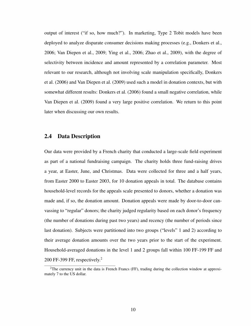
output of interest (“if so, how much?”). In marketing, Type 2 Tobit models have been

deployed to analyze disparate consumer decisions making processes (e.g., Donkers et al.,

2006; Van Diepen et al., 2009; Ying et al., 2006; Zhao et al., 2009), with the degree of

selectivity between incidence and amount represented by a correlation parameter. Most

relevant to our research, although not involving scale manipulation specifically, Donkers

et al. (2006) and Van Diepen et al. (2009) used such a model in donation contexts, but with

somewhat different results: Donkers et al. (2006) found a small negative correlation, while

Van Diepen et al. (2009) found a very large positive correlation. We return to this point

later when discussing our own results.

2.4 Data Description

Our data were provided by a French charity that conducted a large-scale field experiment

as part of a national fundraising campaign. The charity holds three fund-raising drives

a year, at Easter, June, and Christmas. Data were collected for three and a half years,

from Easter 2000 to Easter 2003, for 10 donation appeals in total. The database contains

household-level records for the appeals scale presented to donors, whether a donation was

made and, if so, the donation amount. Donation appeals were made by door-to-door can-

vassing to “regular” donors; the charity judged regularity based on each donor’s frequency

(the number of donations during past two years) and recency (the number of periods since

last donation). Subjects were partitioned into two groups (“levels” 1 and 2) according to

their average donation amounts over the two years prior to the start of the experiment.

Household-averaged donations in the level 1 and 2 groups fall within 100 FF-199 FF and

200 FF-399 FF, respectively.2

2The currency unit in the data is French Francs (FF), trading during the collection window at approxi-mately 7 to the US dollar.

10

Table 2.1: Appeals Scales used in the Field Experiment

 

Table 1: Appeals Scales used in the Field Experiment

Standard Scale

100 FF 150 FF 250 FF 500 FF 1000 FF Other

Prior Donation level Test Scales

1 120 FF 180 FF 250 FF 350 FF 500 FF Other

2 120 FF 200 FF 350 FF 500 FF 750 FF Other

The charity sought to better understand the role of appeals scales in donation behav-

ior, so manipulated it by randomly assigning respondents to receive either a “standard” or

a “test” scale. The standard scale had previously been used for all subjects prior to the

experiment, and thereby helps establish a baseline. Scales all consisted of five suggested

amounts (e.g., 100, 150, 250, 500, 1000 FF for the standard scale), as well as an “Other”

category, which allowed donations below or above all five scale points, or between any

adjacent pair. The test appeals scales manipulated these five suggested amounts; these all

appear in Table 2.1.

The charity thereby implemented a 2 × 2 design: (prior donation) “level 1” or “level

2” × random assignment of either a “standard” or “test” appeals scale. It is important to

note that the charity was collecting real donations, and therefore did not have the luxury of

‘optimally’ designing the scale for the purposes of the experiment, such as orthogonalizing,

including extreme values, and the like. Thus, the points comprising the “test” scale for the

level 2 (higher prior) donation group were higher than those used in the test scale for the

level 1 group. This ‘endogeneity’ is a data limitation over which we had no control, and

our model will take care to treat scales as a collection of anchor points, in part to mitigate

this concern.

11

Table 2.2: Average Donation Amounts and Frequencies

 

Table 2: Average Donation Amounts and Frequencies

Prior Donation

Level Scales

Average Donation Amount Yield Rate

per Household per Occasion

1 Standard 430.2 136.5 31.73%

Test 434.3 137.3 31.61%

2 Standard 844.7 286.2 33.88%

Test 839.5 283.8 33.81%

Two hundred households from each of the four groups were randomly selected for anal-

ysis. Table 2.2 presents descriptive statistics for each, average donation amount (per house-

hold and per occasion), and yield rate. Level 1 and 2 differ substantially in per-household

and in per-occasion average donation amounts; this is unsurprising, as the baseline dona-

tion amount was used by the charity to partition donors into different levels. However, yield

rates are remarkably similar across the four groups, with all between 32% and 34%. More-

over, each of the descriptive statistics - yield rate and both per-occasion and per-household

amount - fails to differ across the standard and test scales, within a donation level (1 or 2).

One might therefore conclude that there were no effects attributable to the use of the test

scale. As our analysis will show, such a conclusion based on aggregated metrics is not only

premature, but highly misleading.

Table 2.3 suggests a clear (aggregate) seasonal pattern in both yield rate and average do-

nation amount: people give more, and more often, at Easter than during June or Christmas.

The difference in yield rates is striking - approximately 34

of respondents donate at Easter

(an important holiday in France), while under 14

do at the other times of year - and these pro-

portions are nearly identical in the level 1 and 2 donation groups (the latter, by construction,

has higher donation amounts across the board). Holding aside any aggregate patterns, there

is nonetheless sizable variation in household-level donation profiles. Table 2.4 presents

donation histories for five households from the level 1/standard scale group, for illustrative

12

purposes; considerable heterogeneity in timing (and some in amounts) is apparent. For

example, households #3, 66, and 118 seem to be a “100FF in Easter, only”, a “not in June”,

and a “never at Christmas” giver, respectively. By contrast, household #148 has no obvious

seasonal or amount pattern. It is these variations in donation patterns - both incidence, and

amount - that we will model, in order to estimate the degree of “pull” of the appeals scale,

which itself will vary across donors.

Table 2.3: Yield Rate and Average Amount of Observed Donations across Seasons

 

Table 3: Yield Rate and Average Amount of Observed Donations across Seasons

Level 1 Level 2

Easter June Christmas Easter June Christmas

Yield Rate 72.8% 18.6% 19.6% 75.3% 17.6% 20.9%

Average Donation 140.1 126.7 129.7 265.0 221.7 215.3

2.5 Model Development

2.5.1 Internal and External Reference Points

The model hinges on two assumptions, as discussed previously: that, for a particular re-

quest, each donor has some (latent) quantity, which serves as an internal referent (rI); and

that the request itself provides a set of alternatives, in the form of the appeals scale, that

serve as external referents (rE). If an appeals scale contains multiple points, we denote the

kth as rE,k.

The internal referent admits different operationalizations; because it is unobserved, it

must be inferred based on data and the model. The reference pricing literature offers several

contenders; among the most common are last price paid (Krishnamurthi et al., 1992; May-

hew & Winer, 1992) and a (perhaps weighted) average of past prices (Kalyanaram & Little,

1994; Lattin & Bucklin, 1989; Mazumdar & Papatla, 2000; Rajendran & Tellis, 1994), and

13

we will empirically compare them. We include two additional specifications that can ac-

count for seasonal donation variations; so, the four (donor-specific) internal reference point

models estimated are: the average of all prior observed donation amounts (IR-1); the last

observed donation amount (IR-2); the average observed donation amount at the same time

of year (IR-3); and the last observed donation amount at the same time of year (IR-4).3

That the external reference points are observable might make them appear simple to

model. This might be so were there only a single requested amount. But, in practice, there

are usually many, and so it is unclear how they exert their “joint pull”: perhaps only the ex-

tremes are noticed; or only those nearest the internal reference have any influence; or some

summary measure of all points (like the average or median); or something else entirely. We

therefore empirically examine five such formulations, where influence is exerted: by all

scale points (ER-1); by the two scale points closest (above and below) the internal referent

(ER-2); by the largest and the smallest scale point (ER-3); by the median (i.e., middle) of

the scale points (ER-4); or by the mean of all scale points, which itself is typically not a

point on the scale (ER-5). We consider such a wide range of possibilities because there is

no prior theory to suggest how a group of referents exert collective influence. In fact, we

view this as among the most intriguing open questions that our data and model can help

address. Note that, when multiple points are presumed to exert influence (as in ER-1, ER-2,

and ER-3), we must also specify the weight associated with each point; we address this in

detail subsequently.

2.5.2 Modeling Scale Attraction Effects

In the absence of any appeals scale - for example, if a potential donor is simply asked

how much s/he would like to give - whether and how much is donated would be influenced

by the internal referent, not any external ones. However, when presented with (the external

3Instead of exponential or geometric time discounting, we used simple averaging, i.e., equal weights.Given the small number of observations per donor (2.99, on average), the difference between the formulationsis minor.

14

referents of) the appeals scale, observed behavior may be affected by both the internal and

external referents. One way to visualize this is that the internal referent is “pulled” by the

external ones, and that these separate pulls (if indeed more than one external referent is

“noticed”, as in ER-1-3) can cumulate in their effects. A simple metric for how influential

a scale point is its “compliance degree,” which we describe next.

2.5.2.1 Compliance Degree

We defineCDk, “compliance degree” of the kth external reference point as the proportional

increase (or decrease) in donation amount from a donor’s internal reference point (rI) to

an external one (rE,k). More formally (with DA = Donation Amount received):

CDk =DA− rI

rE,k − rI(2.1)

For example, if a donor is “planning” to give (i.e., has an internal referent of) $100, but

is asked for $101, he will be very likely to comply, in which case both the numerator and

denominator are $1 and CD1 = 100% (the superscript “1” indicates there was just one

external reference point). However, if the same donor is asked to give $200 more (i.e.,

$300), the donor is less likely to fully comply; if the resulting donation is instead $140,

CD1 = ($140− $100)/($300− $100) = .2, or 20%. In simple language, the donor “came

up 20%” from a $100 baseline. An analogous calculation pertains to external referents

below the internal one.

It is convenient to define the distance, dk, between the kth external and the internal

referent as an incremental/decremental ratio.

distance(dk) =

∥∥rE,k − rI∥∥rI

(2.2)

This allows both compliance degree as well and the pulling amount (described later) to be

expressed as a dimensionless quantity for each donor. This in turn helps to unify the model;

15

for example, it can treat the response of a donor planning to give $10, but asked to donate

$20, similarly to that of one planning to donate $100, but asked for $200.

We will model both upward and downward “compliance degree curves”, which satisfy

three properties:

1) CDk ≈ 1 for dk ≈ 0: “Maximal compliance occurs near donors’ internal referents.”

2) CDk decreases monotonically in dk: “Compliance is worse for requests further from

the internal referent.”

3) CDk ≥ 0: “Compliance can’t be worse than zero.”

Properties 1 and 2 suggest donation is highly responsive to asking for amounts close to

what was ‘planned’ (the internal referent), but increasingly less so for distant amounts.

This is consistent with “latitude of acceptance” in Assimilation-Contrast Theory (Sherif

et al., 1958), which has found prior support in a donation context (Doob & McLaughlin,

1989). Property 3 simply suggests that requests can be ignored, but do not literally repel

donors from a scale point.

There are many ways to specify compliance degree curves satisfying these three proper-

ties, including using fully parametric (e.g., polynomial), semi-parametric, or non-parametric

formulations. We select a translated gamma kernel function, for two reasons. First, it pro-

vides a parsimonious, yet flexible, functional form that naturally satisfies properties 1-3;

this parsimony is important for a heterogeneous account to be identified, given the small

number of responses per donor during the data window. Second, the gamma kernel enables

the pulling amount curves (described later) to follow a unimodal, yet flexibly-shaped, dis-

tribution, which in turn facilitates eventual optimization. Thus, we arrive at an especially

simple form:

16

CDk =exp

(−dk+1

θ

)exp

(−1θ

) = exp

(−d

k

θ

); θ =

exp(βU), rE,k ≥ rI

exp(βD), rE,k < rI(2.3)

where θ > 0 is the gamma kernel scale parameter.

The compliance degree curve follows from a gamma kernel with “shape parameter” 1

and “scale parameter” θ. 4 This is then both translated and normalized - first horizontally

translated by -1 so that it crosses the y-axis, then normalized to have a value of 1 at the

origin - after which it follows a translated gamma kernel, anchored at (0,1) with curvature

determined by the scale parameter. Note that there are actually two different compliance

degree curves, depending on the relative location of the internal and the external refer-

ents. When rE,k ≥ rI , we have an “upward” compliance degree curve, and otherwise a

“downward” one.

Since the scale parameter (θ) must be positive, we specify βU or βD = ln(θ), where

βU and βD are the “upward” and “downward” parameters in (2.3). Figure 2.2 depicts both

curves, which can have a variety of shapes, for different values of βU and βD. However,

βU = βD does not imply identical upward and downward curves, because the domain of

the downward curve is bounded by 100%, since one cannot give less than zero (i.e., a 100%

decrement).4Fixing the shape parameter at 1 yields a non-negative, monotonically decreasing, convex curve (with

regard to the origin), satisfying properties 1-3. Numerous simulations showed recovery of two parameters(both scale and shape) was very poor, suggesting weak identification in data generated to resemble ours.

17

0 50 100 150 200 250 300 350

020

4060

8010

0

Distance(% above)

Com

plia

nce

Deg

ree

(%)

β−2−1 0 1 2

0 20 40 60 80 100

020

4060

8010

0

Distance(% below)

Com

plia

nce

Deg

ree

(%)

β−2−1 0 1 2

A. Upward Compliance Degree B. Downward Compliance Degree

Figure 2.2: Compliance Degree Curves

2.5.2.2 Pulling Amount

The pulling amount (PAk) represents the size of effect exerted by a scale point, a simple

matter of multiplying compliance by the (Euclidean) distance between the internal (rI) and

the kth external reference point (rE,k):

PAk = CDk ×∥∥rE,k − rI∥∥ (2.4)

The pulling amount suggests a trade-off between asking for too little and asking for too

much: If a charity asks too little - that is, just a bit more than the internal referent - com-

pliance (CDk) may be high, but the potential surplus (∥∥rE,k − rI∥∥) is small. On the other

hand, if a charity asks too much, the compliance degree may be low, while the surplus is

large. In light of this trade-off (where the extremes are literally zero), optimizing donation

drives requires considering both elements, that is, asking for a judiciously chosen amount

from each donor.

Each of the two compliance degree curves therefore gives rise to a “pulling amount”

18

curve: rE,k ≥ rI corresponds to “upward” pulling, rE,k < rI to “downward”. The simple

nature of (2.4) implies that these curves also follow a gamma kernel, with shape parameter

2 and scale parameters exp(βU) and exp(βD). As depicted in Figure 2.3, these curves can

have many shapes: the upward pulling curve has domain [0,∞), is unimodal (and thus

has a unique maximum), with zero at the origin and asymptoting to zero for large d (for

any βU ). The domain of the downward pulling amount curve is [0, 1]; it is unimodal (with

unique maximum) if βD < 0, and is monotonically increasing otherwise (with maximum at

1). These internal maxima allow us to derive a closed-form expression for optimal, donor-

specific scale points, discussed in the section on the effect of individually tailored appeals

scales.

0 50 100 150 200 250 300 350

050

100

150

200

Distance(% above)

Incr

ease

in a

mou

nt

β−2−1 0 1 2

0 20 40 60 80 100

020

4060

80

Distance(% below)

Dec

reas

e in

am

ount

β−2−1 0 1 2

A. Upward Pulling Amount B. Downward Pulling Amount

(Internal reference point=100) (Internal reference point=100)

Figure 2.3: Pulling Amount Curves

2.5.2.3 Accumulating Scale Attraction Effects

Because real appeals scales almost always comprise multiple amounts, their effects need to

be somehow combined. Figure 2.4 illustrates the “accumulated pulling amount” accruing

from multiple external referents; to match our empirical application, five external referents

19

are depicted, with two distinct upward and downward curves on either side of the graph.

Here, scale points 1, 2, and 3 are greater than the internal referent (set by convention

to d = 0), so each induces an upward pull on donation amount, tending to increase it.

By contrast, scale points 4 and 5 are lower than the internal referent, tending to pull the

observed donation downward.

The discussion thus far concerns the pulling amount for individual scale points, not how

to combine them. Just as we considered a number of specifications for the effects of the in-

ternal and external referents, we will do so for this combination. Before detailing these, we

highlight one simplifying assumption: that the effect of a particular scale point can be mod-

eled separately from the existence or the location of the others. This is dictated by a data

limitation: the charity did not change scales (over the course of the experiment, nor within

each of the four donation groups), so that identifying interactions between scale points is

not possible. Even were this not the case, such interactions would greatly weaken gamma

kernel parameter (βU and βD) identification, owing to the small number of observations

per donor (and again to the lack of within-donor scale variation during the experiment).

While at first blush such independence assumptions may appear unrealistic, they are

mitigated by the weighted-averaging schemes explored for the “accumulated pulling amount”,

or APA. We examine three: i) the sum; ii) the mean; and iii) the weighted mean of the

pulling amounts. Each is described as follows, along with potential caveats. In general:

APA =K∑k=1

wk × Ik × PAk; Ik =

1, rE,k ≥ rI

−1, rE,k < rI(2.5)

Sum : wk = 1; Mean : wk =1

K; Weighted Mean : wk =

PAk∑Kk=1 PA

k(2.6)

Sum. Simple summation appears to be the most direct way to accumulate the sepa-

rate pulling amounts. However, this specification has two inherent problems. First, the

20

predicted donation amount can lie above the largest, or below the smallest, scale point.

Although this is not impossible, our data contains very few instances in which the donation

exceeds the largest scale point. Second, the effect of including additional scale points can

be overstated (something that, in our data, will not be testable, since the charity fixed this

at 5). For example, given an internal referent of 50, the APA of an appeals scale with four

points of 9, 11, 99, and 101 is about twice as large as for one with two scale points of 10

and 100, which seems decidedly unrealistic.

Mean. The mean specification retains additivity and resolves the two problems with

the sum, but is not without problems of its own, owing to equal-weighting. For example, if

a donor is asked to give $2000 when the planned amount is $100, the effect of such a large

scale point on APA might be small or negligible. However, equal weighting forces a large

scale point like $2000 to have tremendous effect on the APA by substantially lowering the

accumulated pulling amount. A straightforward fix involves the use of a weighted mean,

as follows.

Weighted Mean. This makes use of weights, wk, which one might imagine were es-

timable. Two data limitations prevent this, (once again) the lack of within-donor scale

variation, and that only three different appeals scales (one standard and two test) appeared

in the experiment. For this reason, and because we include heterogeneity βU and βD, even

homogeneous wk proved impossible to estimate.5 Therefore, the weight is set in propor-

tion to the size of pulling amount, based both on conceptual appeal and trial of multiple

alternate schemes (which we do not report here). The key point is that the weighted mean

allows a scale point with a larger pulling amount to contribute more to the total pull, unlike

for either of the previous two specifications.6

5De Bruyn & Prokopec (2011) tried to estimate each scale point’s weight, which they term “absoluteattraction weight”. However, they could estimate only the weight of the smallest of four scale points, whilefixing those of the other three to 1. They attribute this identification problem to the inherent correlationacross suggested donation amounts on the appeals scale (i.e., suggested amounts increase monotonically andare highly correlated).

6In fact, we found model with weighed mean specification (explained next) fits better than that with equalweight mean specification, keeping all other model components the same: The RMSE and MAD of theformer are 0.257 and 0.188 respectively; for the latter, are 0.271 and 0.195.

21

2.5.3 General Model(Type 2 Tobit)

We begin by outlining the general model structure. The model has been set up to allow

a “dimensionless” account of pulling effects, so that heterogeneity can be specified across

the log-scale for donation amount. As discussed earlier, we use a Type 2 Tobit model

(Amemiya, 1985) to jointly account for donation incidence and amount, as follows:

ys∗ = Xsβs + εs (2.7)

ya∗ = ln(rI + APA) +Xaβa + εa, where :

ys = 1, if ys∗ ≥ 0; 0 otherwise

ya = ya∗, if ys = 1; unobserved otherwise

(εs, εa) ∼ BV N(0,Σε); Σε =

1 ρσ

ρσ σ2

The subscripts i and t (for donor and time) are suppressed, and Xs and Xa are covari-

ates in the selection (s) and amount (a) equations, respectively, which we detail below.

In the amount equation, let ya∗ denote the log of the latent donation amount, which

is observed only when a donation is made, that is, when ys is 1, which occurs when the

latent variable ys∗ ≥ 0. The error terms of the selection and amount equations (εs and εa)

follow a bivariate normal distribution; the variance of εs is fixed to 1 for identification. It

is important to note that we model the logarithm of donation amount, for several reasons:

first, it allows εa to be plausibly homoscedastic; second, it allows all effects in the amount

equation to enter multiplicatively; and third, it allows for coefficient heterogeneity to act

on a dimensionless quantity, which we address in detail shortly.

The amount equation (for ya∗) contains two deterministic components. The first is

the sum of a donor’s internal referent (rI) and the accumulated pulling amount (APA).

The second is all factors (Xaβa) that affect the donation, other than those stemming from

22

the appeals scale. Scale-based effects do not appear directly in the selection equation,

because in our data all scales used were set in “reasonable” ranges for every donor (recall

that these were real donors, and the charity was understandably reluctant to alienate them

with unrealistically high requests, or lose funds with low ones). Hypothetically, were all

or many of the suggested amounts exceedingly large, it is possible that the donor would

become annoyed and give nothing. Therefore, although we cannot preclude this possibility

for all data settings, for ours the appeals scale can exercise influence on donation incidence

only indirectly, via the correlation, ρ. [We did estimate a model allowing for scale effects

in selection; the APA coefficient in selection was ns.]

Table 2.4: Examples of Donation Histories for Several Randomly Selected Households

 

Table 4: Examples of Donation Histories for Several Randomly Selected Households

id # 2000 2001 2002 2003

Easter June Xmas Easter June Xmas Easter June Xmas Easter

3 100 0 0 100 0 0 100 0 0 100

20 0 150 0 0 150 0 150 0 0 250

66 200 0 150 200 0 150 150 0 150 250

118 100 100 0 100 100 0 100 0 0 150

148 0 90 0 100 0 100 150 150 100 150

 

 

 

 

 

 

 

 

 

 

 

 

 

 

 

 

 

 

2.5.4 Explanatory variables and Heterogeneity

2.5.4.1 Explanatory variables

Selection Equation

The selection equation contains three types of explanatory variable (Xs), which we detail

subsequently: seasonal indicators, (log of) prior donation, and “level” fixed effects. Ta-

ble 2.3 reveals strong aggregate seasonal variation in donation likelihood, by far highest at

Easter; Table 2.4 suggests household-level variation as well. Previous studies, which were

mostly one-shot, could not account for such seasonal variations, which are critical in our

data. Three dummies - Easter (XEit ), June (XJ

it), and Christmas (XCit ) - represent when the

donation request occurred.

23

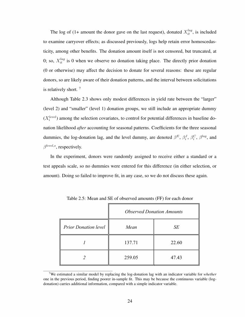
The log of (1+ amount the donor gave on the last request), donated X lagit , is included

to examine carryover effects; as discussed previously, logs help retain error homoscedas-

ticity, among other benefits. The donation amount itself is not censored, but truncated, at

0; so, X lagit is 0 when we observe no donation taking place. The directly prior donation

(0 or otherwise) may affect the decision to donate for several reasons: these are regular

donors, so are likely aware of their donation patterns, and the interval between solicitations

is relatively short. 7

Although Table 2.3 shows only modest differences in yield rate between the “larger”

(level 2) and “smaller” (level 1) donation groups, we still include an appropriate dummy

(X leveli ) among the selection covariates, to control for potential differences in baseline do-

nation likelihood after accounting for seasonal patterns. Coefficients for the three seasonal

dummies, the log-donation lag, and the level dummy, are denoted βE , βJi , βCi , βlag, and

βlevel,s, respectively.

In the experiment, donors were randomly assigned to receive either a standard or a

test appeals scale, so no dummies were entered for this difference (in either selection, or

amount). Doing so failed to improve fit, in any case, so we do not discuss these again.

Table 2.5: Mean and SE of observed amounts (FF) for each donor

 

Table 5: Mean and SE of observed amounts (FF) for each donor

Observed Donation Amounts

Prior Donation level Mean SE

1 137.71 22.60

2 259.05 47.43

7We estimated a similar model by replacing the log-donation lag with an indicator variable for whetherone in the previous period, finding poorer in-sample fit. This may be because the continuous variable (log-donation) carries additional information, compared with a simple indicator variable.

24

Amount Equation

Based on examination of the data and unimproved fit of models including them, seasonal

dummies are not included in the amount equation; the somewhat higher amounts indicated

at Easter in Table 2.3, for example, will be well-explained by other covariates, like lags in

setting “internal” referents (such as in IR-3 and IR-4). Table 2.4 shows far greater house-

hold variation in when to give, not how much; and both Figure 2.5 and Table 2.5 suggest

that household-level seasonal variation in amount is very small for most donors. Similarly,

we do not include a lag for prior donation amount. This may seem paradoxical, but recall

that there is little within-donor variation in observed donation amount, suggesting that that

people do not say, in effect, “I give more than usual last time, so will give less this time,”

or vice versa. 8 Lastly, although donation amount is mainly predicted by a donor’s internal

referent and scale effects, a level dummy (X leveli ) is included to account for the difference

in baseline donation amount between the two groups, denoted βlevel,a.

Figure 2.4: Pulling amounts owing to multiple scale (external reference) points

8To verify this choice, we estimated a series of models with ln(rI+APA+β∗PriorDonation) instead ofthe analogous term in the amount equation. For all reference point models (IR1-4), AIC, BIC, and in-samplefit does not show any improvement.

25

Fre

quen

cy

0 100 200 300 400 500

020

4060

80

Fre

quen

cy

0 50 100 150 200 250 300

050

100

150

200

A. Mean of observed amounts(Level 1) B. SE of observed amounts(Level 1)

Fre

quen

cy

200 400 600 800

050

100

150

Fre

quen

cy

0 100 200 300

020

4060

8010

012

0

C. Mean of observed amounts(Level 2) D. SE of observed amounts(Level 2)

Figure 2.5: Distribution of Mean and SE of observed amounts for each donor

2.5.4.2 Heterogeneity

It is critical, in a model for household-level behavior, to incorporate “unobserved” hetero-

geneity, which we do in several ways. Given the large household-level seasonal donation

variation, we model heterogeneity in the seasonal dummies for the June and Christmas

26

coefficients (βJi and βCi ).9 Our empirical results suggested that household-level seasonal

donation patterns were well reflected in heterogeneity for βJi and βCi , owing perhaps to

much larger variation in giving in June and at Christmas.

Importantly, since our model is primarily meant to capture scale attraction effects, the

two gamma kernel parameters (βUi and βDi ) in the amount equation are heterogeneous.

Imposing heterogeneity on the gamma parameters - especially “upwards”, βUi - is crucial

for formulating tailored appeals scales, which require identifying the request amount with

maximum effect in “pulling” up a donor’s internal referent. If βUi were homogeneous, each

donor’s optimum would be the same percentage above his/her internal referent. This might

still provide a helpful guideline for fundraisers, but presumes all donors are equally ‘elastic’

in being cajoled upwards. Our results, in fact, will strongly weigh against this presumption.

We similarly account for heterogeneity in the “downward” parameter, βDi , though it will

play a lesser role in optimization.

Our formulation therefore specifies four heterogeneous parameters, to be recovered

from the relatively short data window of 7 occasions; the 42.7% aggregate yield rate sug-

gests that about 3 of these 7 requests resulted in donations, on average. Although it may

appear ambitious to account for 4 household-level parameters based on relatively little data,

simulations showed good recovery for all four heterogeneous parameters, and excellent re-

covery of the others.

2.6 Estimation

The full model (see Appendix A) is estimated using Markov chain Monte Carlo methods.

Data augmentation (Tanner & Wong, 1987) converts the model to a Bayesian Hierarchical

Seemingly Unrelated Regression. We obtain posterior draws via Metropolis-within-Gibbs

9Extensive simulations for data matching ours in marginal (summary) statistics failed to recover the trueparameters - mean vector and covariance matrix for βE

i , βJi , βC

i - when the Easter, June and Christmascoefficients were all heterogeneous. Restricting the most common donation period (Easter, with a 74.1%yield rate) to be homogeneous led to nearly perfect parameter recovery.

27

algorithms: Gibbs sampling (Geman & Geman, 1984) if the full conditional of a parame-

ter block is of known form, and Metropolis-Hastings, with a random walk proposal (Chib

& Greenberg, 1995), otherwise. We set diffuse priors for all parameters of interest; de-

tailed procedures appear in Appendix B. All estimates are based on 100,000 draws. We

discard the first 50,000 draws for burn-in, and use the last 50,000 (thinned to every tenth)

to calculate posterior densities. Gelman-Rubin scale reduction factors, using 5 chains with

different stating points, are below 1.1 for almost all parameters, suggesting good conver-

gence (Brooks & Gelman, 1998).

28

Table 2.6: Parameter Estimates for Full Model

 

Table 6: Parameter Estimates for Full Model

Coefficient mean SE 95% HDR

Hom

ogen

eou

s correlation (ρ) -0.387 0.049 ( -0.479, -0.288 )

sd of log amount (σ) 0.296 0.005 ( 0.286, 0.307 )

Easter dummy ( ) 0.782 0.035 ( 0.714, 0.852 )

level dummy in selection ( , ) 0.073 0.039 ( 0.002, 0.156 )

level dummy in amount ( , ) 0.273 0.019 ( 0.237, 0.311 )

log amount lag in selection ( ) -0.131 0.009 ( -0.149, -0.113 )

Het

erog

eneo

us

June dummy ( ) -0.554 0.058 (-0.668, -0.441 )

Christmas dummy ( ) -1.019 0.070 ( -1.163, -0.889 )

“gamma up” ( ) -0.418 0.070 ( -0.563, -0.297 )

“gamma down” ( ) 1.278 0.224 ( 0.858, 1.731 )

sd(June) 0.406 0.071 ( 0.277, 0.554 )

sd(Christmas) 0.831 0.088 ( 0.667, 1.010)

sd(gamma up) 0.478 0.040 ( 0.404, 0.565)

sd(gamma down) 0.932 0.154 ( 0.672, 1.260)

corr(June, Christmas) 0.742 0.108 ( 0.506, 0.906 )

corr(June, gamma up) -0.004 0.050 ( -0.101, 0.094 )

corr(June, gamma down) 0.003 0.050 ( -0.096, 0.103 )

corr(Christmas, gamma up) 0.002 0.049 ( -0.097, 0.096 )

corr(Christmas, gamma down) 0.006 0.050 ( -0.093, 0.102 )

corr(gamma up, gamma down) 0.380 0.145 ( 0.071, 0.626 )

2.7 Results

For brevity, we only present full estimation results for the model with IR-1 (average of

all observed donation amounts) and ER-1 (all scale points), as these provided the best fit

compared with all possible combinations of the other internal and external references point

29

formulations (IR 2-4 and ER 2-5). Table 2.6 summarizes posterior means and standard

errors for all parameters, and detailed model comparison statistics appear in the following

section.

2.7.1 Error Correlation in Selection and Amount equations

The mean of the marginal posterior for the correlation (ρ) between the selection and amount

equation errors is negative (-0.387), and the 95% highest density region does not include

zero. This suggests that unmeasured factors influencing selection are correlated with those

influencing amount, and operate in opposite directions. The size of the correlation is mod-

erate: neither close to 0 nor to 1. This differs from findings in previous research using

related model formulations; for example, Donkers et al. (2006) found the correlation to be

negligible and negative (-0.033), while Van Diepen et al. (2009) found it to be very large

and positive (0.958). A very small correlation fails to help correct for potential selection

biases, and could reflect large, independent sources of error in each equation. Conversely,

a large correlation might suggest important variables omitted in both equations.

It is difficult to generalize such results, since our model accounts for scale attraction

effects, while prior ones do not. We did, however, find significant, moderate, negative

values of ρ across a very wide range of candidate models, indicating that selectivity needs to

be accounted for in our data. One interpretation of this finding, which is apparently robust,

is that, knowing one has donated, the conditional expectation of the donation is smaller.

Thus, models that account for “whether” and “how much” separately may overestimate

total expected yield.

2.7.2 Selection: Seasonality

Comparing the Easter coefficient (0.782) to the means of the (heterogeneous) June and

Christmas coefficients (-0.554, -1.019 respectively) accords with the aggregate benchmark,

that giving is much more likely for Easter than June or at Christmas, on average (a finding

30

that should not be extrapolated beyond French donors to a nationwide “general purpose”

charity.). There is a substantial seasonal heterogeneity: the SD of individual-level param-

eters for June and Christmas are 0.406 and 0.831, respectively. The high (positive) corre-

lation between these individual-level parameters (0.742) largely reflects the fact the yield

rates in June and Christmas are both low (18.1%, 20.3%) and a high proportion of donors

(65.6%) gave at neither time.

2.7.3 Level Dummies and Lagged Log-Amount

The level dummy is only marginally significant (mean 0.073, SE 0.039) in selection, but

significantly positive in amount (mean 0.273, SE 0.019). So, as aggregate statistics suggest,

level 2 donors give more than those in level 1, but with large difference in yield rates. The

coefficient of the log-donation lag in selection is significantly negative (-0.131), indicating

that a larger donation amount last time leads to being less likely to give at all this time.

0 50 100 150 200 250 300 350

020

4060

8010

0

Distance(% above)

Com

plia

nce

Deg

ree

(%)

0 20 40 60 80 100

020

4060

8010

0

Distance(% below)

Com

plia

nce

Deg

ree

(%)

A. Upward Compliance Degree B. Downward Compliance Degree

Figure 2.6: Upward and downward compliance curves at gamma posterior mean

31

0 50 100 150 200 250 300 350

020

4060

8010

0

Distance(% above)

Incr

ease

in a

mou

nt (

%)

0 20 40 60 80 100

020

4060

8010

0

Distance(% below)

Dec

reas

e in

am

ount

(%

)

A. Upward Pulling Amount B. Downward Pulling Amount

Figure 2.7: Upward and downward pulling amount curves at gamma posterior mean

2.7.4 “Pulling Effects”: Gamma Kernel Parameters in Donation Amount

The values of βUi and βDi determine each donor’s degree of compliance (“pull”) to the scale

points above and below the internal referent. Because the domains of the two compliance

curves differ, we should not compare βUi directly to βDi . Instead (and ignoring for the mo-

ment the considerable variation in these across donors), Figure 2.6 shows both compliance

curves at the posterior means of βUi and βDi . The downward compliance curve is far less

‘pitched’ than the upward. This makes intuitive sense: asking for much more than one is

willing to give will eventually result in almost zero compliance, unlike asking for much

less.

The compliance curves are, by construction, monotonic. By contrast, the pulling amount

curves need not be. These are depicted, at the posterior means for βUi and βDi , in Figure 2.7.

The upward pulling amount curve is inverted-U (i.e., unimodal), indicating a single “best

request” value, to which we return later. By contrast, the downward curve decreases mono-

tonically, suggesting that donors tend to give less as the suggested amount decreases (with

lower bound 0).

32

−1 0 1 2

−1

01

2

Up

Dow

n

Figure 2.8: Gamma parameters (up and down) for each donor

Figure 2.8 in some sense encapsulates our main results: the upward and downward

pulling parameters (βUi and βDi ) for each donor. There is clearly a good deal of heterogene-

ity, indicating differing degrees of susceptibility to the appeals scale, despite only modest

differences in prior donation behavior. The upward pulling parameter (βUi ) displays larger

variation (SD 0.93) than the downward (SD 0.48). This might be expected: most every-

one can go along with being asked for less, but people react to being asked for more very

differently.

By allowing a bivariate density for (βUi ,βDi ), the model helps assess overall scale com-

33

pliance. Specifically, we find a substantial correlation (0.380) in these values, suggesting

that donors who are “upward compliant” tend to be “downward compliant” as well. There

is no reason to expect these should be correlated at all, let alone positively, and we believe

this finding to be the first of its kind. This bivariate density for (βUi ,βDi ) leads immediately

to the joint distribution of maximal pulling amounts, those scale points that lead to the

greatest overall effects; we do not call these “optimal”, since a large downward pull is to

be avoided.

Up: Above the Internal Referent (%)

Fre

quen

cy

0 50 100 150 200

050

100

150

200

250

Figure 2.9: Scale point with maximum upward pull

Heterogeneity in (βUi ,βDi ) leads to substantial variation in maximally effective potential

scale point locations, depicted for the “upward” pull in Figure 2.9 (we omit the analogous

34

“downward” distribution, as for most respondents these are zero). The model suggests that

the scale point with maximal upward pull, which varies across donors, ranges from 27.0%

to 198.5%, with a mean of 71.7%, above one’s internal referent, which seems reasonable.10

This non-trivial variation has an important implication: that it may be possible to sub-

stantially increase donations by personalizing an appeals request, based on each donor’s

history. We discuss this possibility later, along with associated calculations.

Figure 2.10 in some sense integrates the key elements of the model, and presents its

main substantive findings in the context of the original data, specifically: How much can

a maximally-effective appeal (either up or down) pull from one’s reference donation? It

depicts, across donors, the maximal percentage increase and decrease (see Appendix E for

derivation). This also allows a direct comparison of the “strength” of upward and down-

ward scale attraction effects, heterogeneously, which was not sensible using (βUi ,βDi ), given

their different domains of operation. The maximum percentage increase ranges from 9.9%

to 73.0% (mean = 26.3%; SD = 7.2%); maximum percentage decrease ranges from 20.5%

to 89.9% (mean = 74.3%; SD = 4.8%). The correlation in these values is 0.298 (echoing the

0.380 value for βUi and βDi ). Figure 2.10 suggests that the maximum percentage decrease

is greater than the analogous increase for most donors: 81.6% of the donors lie above the

diagonal (dotted) line. This is reminiscent of the asymmetric effects in Desmet & Fein-

berg (2003), whose lack of individual-level data precluded any distributions across donors,

and De Bruyn & Prokopec (2011), who only had one-shot (i.e., “before” and “after”) data

unsuited to modeling heterogeneity or carryover effects.

10Discussions with a large university’s fundraising team suggested that the success of “laddering” droppednearly to zero when appeals hit 200% above a donor’s typical or last donation amount.

35

0 20 40 60 80 100

020

4060

8010

0

Maximum Upward Increase(%)

Max

imum

Dow

nwar

d D

ecre

ase(

%)

Figure 2.10: Maximum pulling up and down amounts for each donor

2.8 Model comparison

The data give clear indication of the existence of scale attraction effects. But one might

reasonably question whether these were strongly dependent on the particular form of the

model, four of its elements in particular: 1) internal reference point specification; 2) exter-

nal reference point specification; 3) the importance of including correlation (Type 2 Tobit),

seasonality, and scale effects; and 4) incorporating response heterogeneity. We examine

each of these in some detail, to assess relative “contribution” to overall model fit.

36

With respect to internal reference formulation, we compare four, as described in the

model development section, each donor-specific: the average of all prior donation amounts

(IR-1); the last amount (IR-2); the average of all amounts at the same time of year (IR-

3); and the last amount at the same time of year (IR-4).11 We similarly examine the five

external reference formulations explained earlier: all scale points (ER-1); the two scale

points closest (above and below) the internal referent (ER-2); the largest and the smallest

point in an appeals scale (ER-3); the median (i.e., middle) of all scale points (ER-4); and

the mean of all scale points (ER-5).

We call the model with all the aforementioned components - internal and external ref-

erents; error correlation; seasonality; heterogeneity - the “full model”. Alternative models

include those lacking: error correlation (“no correlation”), scale effects (“no scale effect”),

and both (“simple regression”). We similarly examine the effects of homogenous season-

ality, homogenous scale effects, and both of these.

11For IR-3, IR-4, if we don’t observe donation at a certain time of year in the initialization period (first fullyear, or three data points), we initialize using the mean of the all observed amounts in each group.

37

Table 2.7: In-sample fit of observed donation amounts

 

Table 7: In-sample fit of observed donation amounts 1. Heterogeneous seasonality and scale effects

Full model No correlation No scale effect Simple regression

IR-1 IR-2 IR-3 IR-4 IR-1 IR-2 IR-3 IR-4 IR-1 IR-2 IR-3 IR-4 IR-1 IR-2 IR-3 IR-4

RMSE 0.264 0.287 0.294 0.290 0.276 0.296 0.298 0.301 0.334 0.351 0.320 0.344 0.319 0.331 0.335 0.320

MAD 0.194 0.207 0.215 0.213 0.204 0.215 0.218 0.223 0.229 0.227 0.233 0.228 0.233 0.240 0.238 0.232

LL -2745 -2950 -2910 -2915 -2762 -2923 -2917 -2935 -3201 -3345 -3093 -3270

AIC 5532 5943 5862 5873 5563 5885 5874 5910 6427 6715 6210 6563

BIC 5671 6082 6001 6012 5696 6018 6006 6043 6506 6794 6290 6643

2. Heterogeneous seasonality and Homogeneous scale effects

Full model No correlation No scale effect Simple regression

IR-1 IR-2 IR-3 IR-4 IR-1 IR-2 IR-3 IR-4 IR-1 IR-2 IR-3 IR-4 IR-1 IR-2 IR-3 IR-4

RMSE 0.302 0.312 0.320 0.326 0.308 0.320 0.320 0.330 0.334 0.351 0.320 0.344 0.319 0.331 0.335 0.320

MAD 0.224 0.227 0.233 0.240 0.231 0.235 0.233 0.242 0.229 0.227 0.233 0.228 0.233 0.240 0.238 0.232

LL -3067 -3174 -3102 -3200 -3002 -3090 -3093 -3163 -3201 -3345 -3093 -3270

AIC 6163 6377 6232 6427 6031 6205 6212 6351 6427 6715 6210 6563

BIC 6255 6470 6325 6520 6117 6291 6298 6438 6506 6794 6290 6643

3. Homogeneous seasonality and Heterogeneous scale effects

Full model No correlation No scale effect Simple regression

IR-1 IR-2 IR-3 IR-4 IR-1 IR-2 IR-3 IR-4 IR-1 IR-2 IR-3 IR-4 IR-1 IR-2 IR-3 IR-4

RMSE 0.266 0.286 0.296 0.291 0.276 0.296 0.298 0.301 0.334 0.351 0.320 0.345 0.319 0.331 0.335 0.320

MAD 0.196 0.208 0.217 0.214 0.204 0.215 0.218 0.223 0.229 0.228 0.233 0.228 0.233 0.240 0.238 0.232

LL -3062 -3242 -3314 -3270 -3169 -3330 -3348 -3366 -3608 -3718 -3508 -3690

AIC 6152 6512 6656 6568 6364 6686 6721 6758 7234 7454 7035 7399

BIC 6245 6605 6749 6661 6450 6773 6807 6844 7294 7514 7094 7459

4. Homogeneous seasonality and scale effects

Full model No correlation No scale effect Simple regression

IR-1 IR-2 IR-3 IR-4 IR-1 IR-2 IR-3 IR-4 IR-1 IR-2 IR-3 IR-4 IR-1 IR-2 IR-3 IR-4

RMSE 0.304 0.313 0.320 0.328 0.308 0.320 0.320 0.330 0.334 0.351 0.320 0.345 0.319 0.331 0.335 0.320

MAD 0.226 0.228 0.233 0.241 0.231 0.235 0.233 0.241 0.229 0.228 0.233 0.228 0.233 0.240 0.238 0.232

LL -3380 -3462 -3508 -3551 -3428 -3515 -3518 -3589 -3608 -3718 -3508 -3690

AIC 6781 6945 7037 7125 6875 7049 7056 7197 7234 7454 7035 7399

BIC 6854 7018 7110 7198 6941 7116 7122 7263 7294 7514 7094 7459

38

Table 2.8: In-sample fit of observed donation amounts (Full model with IR-1)

 

Table 8: In-sample fit of observed donation amounts (Full model with IR-1)

RMSE MAD LL AIC BIC

ER-1: All five scale points 0.264 0.194 -2745 5532 5671 ER-2: Two closest scale points from the internal referent 0.280 0.195 -2871 5784 5923

ER-3: Largest and smallest scale points 0.293 0.208 -2899 5840 5980 ER-4: Middle scale point 0.285 0.209 -2932 5906 6045 ER-5: Mean of all five scale points 0.312 0.217 -3078 6198 6337

 

For model comparisons, owing to short donation histories (which preclude ‘squander-

ing’ an entire year for prediction purposes), we compare fit in-sample. “Fit” is assessed via

mean absolute deviation (MAD) and root mean square error (RMSE) for donation amount

predictions, which appear in Tables 2.7 and 2.8. Table 2.7 shows that the proposed model

(the “full” model with IR-1, ER-1 and both seasonal and scale effect heterogeneity) pro-

vides a better fit than all alternatives; moreover, including error correlation and scale effects

improves fit regardless of internal reference formulation (IR1-5) and the inclusion of het-

erogeneity. Table 2.7 also allows us to judge relative contribution to overall model fit:

scale effects easily best both correlation and seasonality. For example, in subtable 2.7-1,

which incorporates heterogeneity in both seasonality and scale effects, failing to account

for scaling effects inflates RMSE and MAD approximately 30%; the corresponding figure

for removing correlation alone is ≈ 5%; and for dropping heterogeneity entirely, ≈ 20%.

Even in the final subtable (2.7-4), for homogeneous seasonality and scale effects, discard-

ing scale attraction inflates RMSE and MAD by approximately 10%; dropping correlation,

about 1%. These comparisons suggest that scale attraction effects appear to explain more

variation in giving than those typically modeled in prior donation research combined, al-

though it will require additional data applications and distinct settings to verify whether

this holds generally.

In terms of internal reference point specification, IR-1, the average of all prior donation

39

amounts appeared to dominate across the board. The degree of dominance was not triv-

ial, sometimes hovering near 10%. To our knowledge, such a test of ‘internal’ referents is

unique in donation contexts, and we know of no prior theory that would have anticipated

it. We found as well that allowing for heterogeneous scale effects (subtables 1 and 3) pro-

vides superior fits compared with analogous homogeneous scale effects models (subtables

2 and 4). However, allowing heterogeneity in seasonality parameters offered rather small

increases in fit. So, although heterogeneity is itself important, overall, it is much more so

in terms of scale effects.

Based on the results of Table 2.7, we restrict our attention to the “full” model with

IR-1, and Table 2.8 summarizes fits of five distinct external reference specifications (ER

1-5) for this model. ER-1, with all five scale points included, clearly dominates. We

hesitate to term this a general finding, as the charity did deliberately choose all scale points

to be “reasonable”, since they were understandably more focused on revenue than testing

reference point theories. Regardless, the “full” model with IR-1 and ER-1 was verified,

using all discussed metrics, to provide the best fit to the data among the 2×2×2×2×4×5

(scale effects?; scale effect heterogeneity?; seasonality heterogeneity?; error correlation?;

IR1-4; ER1-5) design.

To guard against concluding in favor of a potentially overparameterized model based

on in-sample fit, we report log-likelihood (LL), AIC, and BIC.12 LL is based on the Tobit 2

likelihood, calculated at parameters’ posterior means. The proposed model has the largest

LL and smallest AIC and BIC, consistent to the in-sample fit test result.

12We do not report two common Bayesian model comparison measures, the Bayes factor and DIC, forthe following reasons. The marginal likelihood (on which the Bayes factor is based) is well known to besensitive to prior specification and calculation method. We in fact computed marginal likelihoods underseveral different diffuse priors and common calculation methods, finding it highly variable across them. DICis also not appropriate here, as it has multiple plausible definitions in missing data models (Celeux et al.,2006). Parameters for AIC and BIC are based on Level-I for homogeneous parameters and Level-II forheterogeneous ones. AIC and BIC are included for comparison purposes only, not as definitive bases forBayesian model selection.

40

2.9 Illustrative Application: Effect of individually tailored appeals

scales

We conclude with a preliminary examination of setting a superior appeal. While a laudable

goal might be to devise optimal donor-specific appeals scales or even a single optimal scale

applicable to the entire donor pool, the nature of the available data do not permit this, for a

number of reasons. Foremost among these was that the scales used by the charity changed

neither during the course of the experiment nor across the four donation groups ([level 1,

2] × [test, standard]). Although the existence (and nature) of scale attraction effects was

strongly verified, this lack of within-donor variation made identifying interactions between

scale points impossible, since they were perfectly confounded with the experimental con-

ditions themselves. Such interactions are necessary to avoid placing all points in a k-point

scale at the same “optimal” spot, an obvious absurdity never seen in real appeals scales. De-

tailed simulations (available from the authors) verified these claims, which we view simply

as a data limitation stemming from constraints put on the charity provider.

We instead focus on choosing a single optimum request - often referred to as an attempt

to “ladder” an individual donor - and the effect of tailoring these to each donor, as opposed

to using a common best ladder (increase percentage over the internal referent) for each,

the ubiquitous practice among real fundraisers, even those with donation histories at their

disposal. Finding a single optimal request may appear paradoxical, but we must remember

that the charities that use appeals scales do not vary them across individuals - the very issue

that provoked the modeling effort here - and moreover would never have reason to ask for

less than an internal referent, given its small pulling effect.13

13Although neither our data nor model allows us to rectify this issue, it’s unclear whether using multiplescale points is useful in charitable appeals, let alone how many. An appeals scale with multiple points mightbe beneficial when the charity cannot estimate donors’ internal referents, as when soliciting from first-timedonors. If there is wide variation in internal referents, a suitably-spaced appeals scale may help donors finda reasonable anchoring point. Regardless, whether it is beneficial to present multiple scale points to regulardonors is an empirical question awaiting suitable data, in which the number of scale points is systematicallyvaried.

41

Given these data limitations, we conducted a simulation study involving a single re-

quest amount, and a three-period (i.e., one full year) look-ahead. We immediately discov-

ered that seasonal patterns, which were exceedingly strong in our data, vastly swamped

any benefit of potential strategies of “let’s ask for less now, so they’ll give somewhat less,

and use that carryover to make them more likely to give again next time.” It simply did

not matter. Thus, the “three-period look-ahead” optimization, which involved discrete dy-

namic programming, gave results identical to the three “myopic one-period look-ahead”

optimizations, on which we report. Our sole focus, as stated earlier, is quantifying the re-

sults of the appeal itself when it is generated heterogeneously, based on donation history,

as opposed to a “one ladder fits all” strategy.

To run the simulation, the optimal suggested amount and the expected value of donation

amount are calculated, based on βU . The optimal external referent, rE∗, can be calculated

by solving a first-order condition for the upward pulling amount, PA (see Appendix C for

derivation).

rE∗ = (exp(βU) + 1)rI (2.8)

The expected value of donation amount can also be calculated analytically. We use the

generic symbols νs and νa for the deterministic parts in the selection and donation amount

equations in (2.7). Because ya∗ is a logged quantity, it needs to be exponentiated to calculate

the expected donation amount, which is as follows (see Appendix D for derivation):

E[exp(ya)] = exp

(νa +

σ2

2

)× Φ(νs + σρ) (2.9)

Three different types of appeals were used in the simulation: i) a “pseudo” appeal, with

no suggested amount; ii) a group-level optimized suggested amount; and iii) an individually

customized suggested amount. In the first case, where no external referent is provided, we

presume donors hew to their internal referents; this thus serves as a convenient benchmark.

42

The group-level request is the single common value that would optimize overall donations,

given the heterogeneous distribution of βUi . Individual-level amounts are calculated from

each donor’s βUi separately. Simply put, the first scenario does not account for scale effects

at all; the second type does, but presumes a common “best request” for everyone (as per

current practice in the fundraising industry); and the third accounts for individual-level

scale effects.

In each scenario, we compare the expected donation amount of 1,000 donors in each

of two hypothetical groups (level 1 and 2). These hypothetical donors are generated via

the homogeneous parameters (e.g., group dummies) and draws from the joint multivariate

normal density obtained from the field experiment (Table 2.6). One challenge in conducting

a simulation study is that we cannot “observe” internal reference points and lag-amounts

for hypothetical donors. We thus use the group-wise mean of all observed amounts in the

real data as a proxy for the group-wise internal reference points for hypothetical donors. As

a proxy for the last donation amount (the lag amount in each period), we use the group-wise

mean of all observed amounts for Easter, in June, and at Christmas. Then, for each period,

the proportion of hypothetical donors giving in each period was set to reflect the response

rate in the real data.

Table 2.9: Expected value of average donation amount in simulation

 

Table 9: Expected value of average donation amount in simulation

Level 1 Level 2

Easter June Xmas Level 1Total

Easter June Xmas Level 2Total

Individually Tailored Request

127.6 28.6 32.2 188.4 321.3 70.0 81.1 472.4

Group-wise Request

124.8 28.0 31.4 184.2 314.7 68.5 79.4 462.6

No suggested amount

100.4 22.5 25.3 148.3 252.8 55.0 63.8 371.5

Table 2.9 shows the effect of an individually tailored appeals scale compared to a group-

wise appeals scale. Improvements (from the group-wise to the individual-level appeals

43

scale) are larger in the level 2 group (than in level 1), because their baseline donation

amounts are higher. Likewise, Easter entails the largest increase due to its much higher

response rate. The full-year expected donations, for an average level 1 and level 2 donor

combined, are 519.8FF, 646.8FF, and 660.7FF, for the “no appeal”, “group appeal”, and

“individual appeal” cases, respectively. The latter two both show marked improvement

over “no appeal”, 24.4% and 27.1%, respectively, offering a “scale-free” (if we may use

that term) assessment of the power of making a donation request. By contrast, making

an individually-tailored request offers a more modest improvement of 2.2% over a group-

wise request. While this may seem comparatively small, it is certainly not so for charities.

Moreover, charities are already making common group-wise requests (albeit, probably not

close to optimal ones), so the question is how to leverage the individual donation histories

they already have to boost total yield more. Here, we have done so by simultaneously

modeling the effects of such a request on both yield rate and donation amount, as well

as the intercorrelation of their unobserved influences (errors), and donor-level response

heterogeneity.

Our simulation study should be taken as an illustrative exercise awaiting more detailed

field data from a properly orthogonalized, custom design (although one wonders which

charity will risk potential losses from such an experiment). Most notably, the nature of our

data made it impossible to optimize an entire scale. However, the results clearly suggest

both the importance of making an appropriate request, and of incorporating heterogeneity.

We believe the platform developed here would allow for optimal “laddering,” which is the

dominant practice in real fundraising, for individual donors

2.10 Conclusion

Charities have long relied on appeals scales as cornerstones of their donation requests,

though with little theory or measurement to guide them. In that light, the model developed

here offers a heterogeneous, joint account of donation incidence and amount, addressing

44

potential selectivity in modeling these separately. Importantly, different specifications for

internal and external reference point theories can be assessed via model comparison.

Results suggest that variation across donors in scale attraction effects and seasonal do-

nation patterns can be substantial. Such a finding depends critically on the availability of

donation histories, explaining its absence from prior studies. A moderate, significantly neg-

ative, correlation between donation incidence and amount indicates the selectivity-based

pitfalls of separately modeling incidence and amount. In terms of internal and external

referents, we found that the mean of the previous donation amounts (internal referents)

and including all points in an appeals scale (external referents) offered the best fit with

our data. Importantly, the model allowed for a preliminary exploration of laddering, the

common practice of asking for successively greater donation amounts.

Our study has some notable limitations, stemming mainly from the data. The charity

that designed and carried out the study was not interested in optimal experimental practice,

but in gaining some degree of insight within the context of a live donation drive. So,

there is a potential issue with appeals scale amounts roughly tracked prior donation level

in each segment. Second, because of the lack of group- and time-wise variation in appeals

scale, the weight of each scale point - let alone any potential interactions among them -

simply cannot be estimated; nor could the optimal number of points be ascertained. Third,

because the appeals scales in the experiment contained only ‘reasonable’ amounts, effects

of extreme scale points, such as ignoring them or even of alienating donors, could not be

measured. Despite these data limitations, the model showed clear and strong evidence for

scale attraction, in both upward and downward directions, and that the degree of attraction

varied greatly across donors.

Some of the data limitations suggest clear directions for future experimental and field

research. First and foremost would be some scheme for orthogonalizing appeals scale

amounts across various donor groups, and even the number of points on the scale, so that

a truly “optimal” scale for each donor can be devised. Key to doing this is accounting for

45

interactions among scale points, which is necessary to avoid “bunching up” in optimization.

Future research might also identifying subtleties of weighting: do some consumers ignore

endpoints, while others anchor on them? Experiments could similarly include extreme

scale points, to see whether they are ignored entirely, lead respondents not to donate at all,

or something more subtle. Any such data could be analyzed through variants of the basic

framework employed here, and would help validate cross-study norms about scale point

attraction effects, as well as fashion individually-tailored, multi-period laddering plans.

46

2.11 Appendix

A. Full Model Specification

As discussed above, we can write the entire model as follows (i = donor; t = time):

ys∗it = βEXEit + βJi X

Jit + βCi X

Cit + βlagX lag

it + βlevel,sX leveli + εsit

ya∗it = ln(rIit + APAit) + βlevel,aX leveli + εait, where :

ysit = 1, if ys∗it ≥ 0; 0 otherwise

yait = ya∗, if ysit = 1; unobserved otherwise

APAit =K∑k=1

wkit × Ikit × PAkit; wkit =PAkit∑Kk=1 PA

kit

, Ikit =

1, rE,ki ≥ rIit

−1, rE,ki < rIit

PAkit = CDkit ×

∥∥∥rE,ki − rIit∥∥∥

CDkit = exp

(−d

kit

θi

); θi =

exp(βUi ), rE,ki ≥ rIit

exp(βDi ), rE,ki < rIit

, dkit =

∥∥∥rE,ki − rIit∥∥∥

rIit

(εsit, εait) ∼ BV N(0,Σε); Σε =

1 ρσ

ρσ σ2

βi ∼MVN(∆,Σβ), where βi = (βJi , β

Ci , β

Ui , β

Di )

Note that the internal reference point, rIit, for donor i can change over the course of the

experiment, and is subscripted accordingly. However, since the appeals scale for donor i

does not change over time, the kth external reference point for a donor i, rE,ki , lacks a t

subscript. Again, the variance of εs is fixed to 1 for identification. Finally, the vector of

heterogeneous parameters (βi) follows a multivariate normal distribution with mean µβ and

full-rank covariance matrix Σβ .

47

B. MCMC Algorithm and Priors

Here we present the prior distributions and sampling algorithm used in estimation. Be-

cause the requirement that setting error variance of the binary probit model (for donation

incidence) be set to one ruins useful conjugacy properties, we instead make random draws

from the unidentified space, as suggested by Edwards & Allenby (2003), and report post-

processed estimates. Below, we specify Σε in the unidentified space as

Σε =

σ2s ρσsσa

ρσsσa σ2a

1. Data Augmented Likelihood

n∏i=1

T∏t=1

[(ys∗it , ya∗it )|βh, βi,Σε]×

n∏i=1

[βi|µβ,Σβ]

where βh = (βE, βlag, βlevel,s, βlevel,a) is a vector of homogeneous parameters and βi =

(βJi , βCi , β

Ui , β

Di ) is a vector of heterogeneous parameters.

2. Prior Distribution

We use proper but diffuse priors.

(1) βh ∼MVN(M,V ), where M = 0, V = 104I

(2) Σε ∼ IW (νΣε , VΣε), where νΣε = 5, VΣε = 5I

(3) ∆ ∼MVN(∆, A), where ∆ = 0, A = 104I

(4) Σβ ∼ IW (νΣβ , VΣβ), where νΣβ = 7, VΣβ = 7I

48

3. Posterior Distribution

n∏i=1

T∏t=1

[(ys∗it , ya∗it )|βh, βi,Σε]×

n∏i=1

[βi|µβ,Σβ]× [βh|M,V ]× [Σε|νΣε , VΣε ]×

[∆|∆, A]× [Σβ|νΣβ , VΣβ ]

4. Sampling Algorithm

Step 1. Draw ys∗it and ya∗it (Data augmentation step)

[(ys∗it , ya∗it )|ysit, yait, βh, βi,Σε]

1. If ysit = 1 then yait is observed. We set ya∗it = yait and draw ys∗it from the truncated normal

distribution below:

TN(βEXEit + βJi X

Jit + βCi X

Cit + βlagX lag

it + βlevel,sX leveli +

ρσsσa

[yait − (ln(rIit + APAit) + βlevel,aX level)], (1− ρ2)σ2s), y

s∗it ≥ 0

2. If ysit = 0 then yait is not observed. We draw (ys∗it , ya∗it ) by following steps

a. Draw ys∗it from TN(βEXEit + βJi X

Jit + βCi X

Cit + βlagX lag

it + βlevel,sX leveli , σ2

s), ys∗it < 0

b. Draw ya∗it conditional on ys∗it from normal distribution below:

N(ln(rIit + APAit) + βlevel,aX leveli +

ρσaσs

[ys∗it − (βEXEit + βJi X

Jit + βCi X

Cit + βlagX lag

it + βlevel,sX leveli )], (1− ρ2)σ2

a)

Step 2. Draw βi

49

[βi|βh,Σε,∆,Σβ] ∝T∏t=1

[(ys∗it , ya∗it )|βh, βi,Σε]× [βi|∆,Σβ]

The full conditional distribution is also of unknown form. Therefore, we use a Metropolis-

Hastings algorithm with a normal random walk proposal to make draws.

Step 3. Draw βh

[βh|{βi},Σε] ∝n∏i=1

T∏t=1

[(ys∗it , ya∗it )|βh, βi,Σε]× [βh|M,V ]

Again, we use a Metropolis-Hastings algorithm with a normal random walk proposal to

make draws.

Step 4. Draw Σε

[Σε|βh, {βi}] ∝n∏i=1

T∏t=1

[(ys∗it , ya∗it )|βh, βi,Σε]× [Σε|νΣε , VΣε ]

∝n∏i=1

T∏t=1

BV N

ys∗it

ya∗it

| usit

uait

,Σε

× IW (νΣε , VΣε)

[Σε|βh, {βi}] ∼ IW (νΣε , VΣε),

νΣε = νΣε + nT,

VΣε = VΣε +n∑i=1

T∑t=1

ys∗it − usit

ya∗it − uait

× ys∗it − usit

ya∗it − uait

T

where

usit = βEXEit + βJi X

Jit + βCi X

Cit + βlagX lag

it + βlevel,sX leveli

uait = ln(rIit + APAit) + βlevel,aX leveli

50

Step 5. Draw ∆

[∆|{βi},Σβ] ∝n∏i=1

[βi|∆,Σβ]× [∆|∆, A] ∝MVNnk(B∗|[Z ⊗ Ik]∆∗, In ⊗ Σβ)

×MVNnk(∆∗|∆, A)

where βi is a vector of length k,

B =

βT1

βT2...

βTn

, B∗nk×1 = vec(BT ), Z =

ιT1

ιT2...

ιTn

, ∆∗ = vec(∆T )

[∆∗|{βi},Σβ] ∼MVNnk(∆∗|∆, A)

where ∆ = A([Z ⊗ Σ−1β ]B∗nk×1 + A−1∆), A = [(ZTZ)⊗ Σ−1

β + A−1]−1

Step 6. Draw Σβ

[Σβ|{βi},∆] ∝n∏i=1

[βi|∆,Σβ]× [Σβ|νΣβ , VΣβ ] ∝MVNnk(B|Z∆, In,Σβ)× IW (νΣβ , VΣβ)

[Σβ|{βi},∆] ∼ IW (νΣβ , VΣβ)

where νΣβ = νΣβ + n, VΣβ = VΣβ + (B − Z∆)T (B − Z∆)

51

C. Single Optimal Appeal

The single optimal appeal is that (scale) point (rE∗) that maximizes the log of the latent

donation amount (ya∗). Clearly, rE should be greater than rI and maximizes the upward

pulling amount (PA), so that rE∗ solves a first order condition (PA with respect to rE).

Subscripts for donors and times (i, t) are suppressed for simplicity.

ya∗ = ln(rI + PA) +Xaβa + εa

PA = exp

(−dθ

)(rE − rI), d =

rE

rI− 1, θ = exp(βU)

FOC :∂PA

∂rE= 0

rE∗ = (θ + 1)rI = (exp(βU) + 1)rI

D. Expected Donation Amount

Following the Type 2 Tobit model specification, let ys∗ and ya∗ be the latent dependent

variables in the selection and the amount equations, and ys and ya be their observed coun-

terparts in (2.9). We set νs, νa to be deterministic parts of each equation and εs, σεa to be

stochastic parts.

Now we have the system of equations:

ys∗ = νs + εs

ya∗ = νa + σεa

Because the errors are correlated, we can re-write the system as (writing εs as ε):

ys∗ = νs + ε

ya∗ = νa + σ(ρε+ ρz)

52

where z is a standard normal draw uncorrelated with ε, and ρ =√

1− ρ2. We want to

calculate E[exp(ya)], the expected donation amount, and so merely integrate over the two

uncorrelated errors, z and ε:

E[exp(ya)] =

ε=∞∫ε=−νs

z=∞∫z=−∞

exp[νa + σ(ρε+ ρz)]φ(z)φ(ε)dzdε

= exp(νa)×ε=∞∫

ε=−νs

exp(σρε)φ(ε)dε×z=∞∫

z=−∞

exp(σρz)φ(z)dz

The second term can be calculated by completing the square:

ε=∞∫ε=−νs

exp(σρε)φ(ε)dε =

ε=∞∫ε=−νs

exp(σρε)1√2π

exp

(−ε

2

2

)dε

=

ε=∞∫ε=−νs

1√2π

exp

(−(ε− σρ)2

2

)dε× exp

((σρ)2

2

)Let u = ε− σρ

=

u=∞∫u=−νs−σρ

1√2π

exp

(−u

2

2

)du× exp

((σρ)2

2

)= Φ(ν2 + σρ)× exp

((σρ)2

2

)

The third term can also be calculated by completing the square:

z=∞∫z=−∞

exp(σρz)φ(z)dz =

z=∞∫z=−∞

exp(σρz)1√2π

exp

(−z

2

2

)dz

=

z=∞∫z=−∞

1√2π

exp

(−(z − σρ)2

2

)dz × exp

((σρ)2

2

)= exp

((σρ)2

2

)

53

Putting this all together, the expected value of donation amount is:

E[exp(ya)] = exp(νa)× Φ(ν2 + σρ)× exp

((σρ)2

2

)× exp

((σρ)2

2

)= exp(νa)× Φ(ν2 + σρ)× exp

(σ2ρ2

2

)× exp

(σ2(1− ρ)2

2

)∵ ρ =

√1− ρ2

= exp

(νa +

σ2

2

)× Φ(ν2 + σρ)

E. Distance ratio and the incremental/decremental amount, calculated at the scale

point with the maximum pulling amount

1.Upward pulling amount

When rE ≥ rI , the upward pulling amount PAU follows:

PAU = exp

(−dUθ

)(rE − rI), dU =

rE

rI− 1, θU = exp(βU)

The scale point with maximum upward pulling amount (rE∗) can be calculated by solving

first order condition of PAU with respect to rE .

rE∗ = (θU + 1)rI = (exp(βU) + 1)rI

At the scale point of rE∗, the incremental ratio in distance (d∗U ) is determined to be exp(βU)

and the maximum incremental ratio in the amount to be as follows:

exp(− d∗U

exp(βU )

)(rE∗ − rI)

rI= exp(−1) exp(βU)

54

2. Downward pulling amount

When 0 ≤ rE ≤ rI , the downward pulling amount PAD follows:

PAD = exp

(−dDθ

)(rI − rE), dD = 1− rE

rI, θD = exp(βd)

The scale point with maximum downward pulling amount (rE∗) can be calculated by solv-

ing first order condition of PAD with respect to rE . We should note that there is a corner

solution if βD > 0.

rE∗ =

(1− θD)rI = (1− exp(βD))rI , βD ≤ 0

0, βD > 0

At the scale point of rE∗, the decremental ratio in distance (d∗D) is determined to be

exp(βD), βD ≤ 0

1, βD > 0

And the maximum decremental ratio in the amount is determined to be as follows:exp

(− d∗U

exp(βU )

)(rI−rE∗)

rI= exp(−1)− exp(βU), βD ≤ 0

exp

(− d∗U

exp(βU )

)(rI−rE∗)

rI= exp

(− 1

exp(βD)

), βD > 0

55

CHAPTER III

Modeling Mate Choice Behavior: A Two-Stage Mate

Choice Model with Potentially Non-Compensatory

Decision Rules

3.1 Abstract

In this research, we develop a two-stage mate choice model that allows us to empirically

evaluate the evidence in favor of alternative decision rules using data from an online dat-

ing service provider in the US. The proposed model captures the intrinsically multistage

behavior involved in many online transactions, but in particular dating, where one decides

which profiles to browse and then, conditional on having browsed, whom to write to, if any-

one. Here, we account for these two distinct activities by modeling the binary decisions (of

browsing and writing). The model can accommodate compensatory and non-compensatory

decision rules in each stage; it allows decision rules to differ across stages; different at-

tributes can be modeled as having distinctly different utility ‘shapes’; and heterogeneity in

rule use across site users provides interpretable profiles of different types of mate-seeking

behavior. Finally, and most importantly, we directly model the utility functions of attributes

to identify and compare attribute-level decision rules (“deal-breakers” and “deal-makers”)

over two stages.

56

3.2 Introduction

There is currently great interest among marketers, policymakers, and government funding

agencies in models of human decision-making; the hope is that better understanding of how

people make decisions may allow us to develop more effective policies aimed at meeting

the needs of a diverse consumer pool, as well as potentially changing behavior (e.g., be-

ing more charitable, using fewer resources, etc.) In consumer behavior and social science

research, the standard approach is to decompose variation in some individual outcome of

interest into portions attributable to different “explanatory” covariates. Causal relation-

ships are typically attributed to variables rather than to human actors, whose behavior is

contingent and often difficult to measure. In social science research in particular, the sta-

tistical model used in the analysis is rarely a plausible model of the underlying behavior or

decision-making process that gave rise to the social phenomenon under investigation; as a

result, these analyses are often divorced from the actions or activities that led to a partic-

ular outcome. To understand consumer needs or fashion effective interventions, we need

plausible models of how individuals navigate their social and physical environment.

Researchers in the field of marketing modeling have, for the past 30 or more years,

worked out sophisticated models of decision-making, but these have rarely been applied to

social contexts, for example, how people choose among potential partners, neighborhoods,

jobs, or entrees in a cafeteria. Among the many reasons for this are cultural differences

in emphasis (e.g., drivers of individual-level behavior in marketing vs. “big picture” un-

derstanding of entire systems in political science and sociology), data availability (detailed

databases in marketing vs. more macro-level variables in social science), and degree of em-

phasis on methodology per se. Given that both fields concern themselves with understand-

ing human behavior, there is fertile territory at their intersection: extending individual-level

choice models from marketing which tend to involve one decision-maker picking from a

known set of options under measured conditions to a variety of thorny, open problems in

sociology and cognate disciplines.

57

Specifically, the overarching goal of this study is to extend statistical techniques and

theoretical models from marketing and choice theory to studies of sociologically relevant

decision-making, with a particular emphasis on what is arguably the most important deci-

sion an individual can make: mate choice. In contrast to existing work in social science,

we develop a statistical model of choice behavior that allows for an actor with partial infor-

mation, uncertainty about the most desirable outcome, and difficulty comparing more than

a handful of alternatives based on a small number of attributes (see Shocker et al., 1991,

for review). Importantly, the proposed multistage choice model allows for the possibility

of compensatory and non-compensatory screening rules (as discussed later), and different

attributes may be evaluated using different rules.

As mentioned earlier, the substantive application is mate choice, a subject with deep

roots in social science, but only recently amenable to individual-level modeling. Here,

our data stem from an online dating site, an increasingly common way to meet potential

dating or marriage partners. Between 1995 and 2005, there was a rapid increase in the

number of opposite-gender couples who met their partners online (Rosenfeld & Thomas,

2012). A study commissioned by Match.com in 2010 reported that 1 in 6 couples married

within the past three years met their partner on an online dating site, and 1 in 5 people

have dated someone they met on an online dating site (Chadwick, 2010). The increased

availability of behavioral data from online dating web sites has led to a number of studies

to use patterns of early stage interaction online that is, who browses, contacts, or responds

to whom to estimate models of mate choice (Hitsch et al., 2010; Lin & Lundquist, 2013).

However, in all cases, the key focus is on “preferences”, as reected in the relative magnitude

and signicance of coefficients in a statistical model. The statistical technique used in these

studies assumes a single-stage decision process, in which mate-seekers with unlimited time

and computational resources consider every single potential mate in their metropolitan area

using a compensatory model. Thus, despite the behavioral nature of the online dating data,

past empirical analyses do not in any way represent the underlying activities that give rise

58

to choice outcomes. Researchers instead impose the same and statistical techniques that

have been used for decades to analyze survey data, but which are arguably implausible for

online dating and a variety of related data settings.

Behavioral data provide new opportunities to develop theoretical models of individual

choices, but this requires an expanded repertoire of statistical models. Compared with tra-

ditional sources of information about how individuals search among potential mates (e.g.,

observed matches or preferences revealed in surveys), online dating activities provide far

richer information understanding mate choice, for two reasons: (1) researchers have ac-

cess to individual-level, longitudinal interaction histories for each participant, including a

standardized (or at least stable) array of demographic covariate information for browsed

and written-to profiles, which helps statistically nail down accurate mate preferences for

users; and (2) the online world facilitates observation of all intermediary steps undertaken

by each user while on the site, such as login history, overall time spent, detailed browsing

history, profiles viewed and rejected, etc. Although demographic information was always

potentially, if somewhat spottily, available using traditional sources, it is this truly novel

information on intermediary behaviors that can shed light on both how matching happens

and on users decision process, a level of analysis simply not possible solely using records

final matches alone.

3.3 Model development

The main objective in model development is to understand how two-sided matching takes

place when there are many, interacting searchers/decision-makers, each with his or her own

preferences, which express themselves as utilities. These functions (i.e., utilities based on

attributes), as discussed in full later, should not be presumed to have constant marginal

disutility; that is, “a year is a year” for age or that each inch in height matters as much as

any other. Although the model is tested on dating site data, the overarching objective is

59

broader, and concerns how to capture multistage, highly multiattribute utility functions in

an estimable and relatively parsimonious manner, when we cannot simply presume strict

linearity (or linear-additivity) in the components of utility across their entire ranges. We

next discuss some extant hypothesis regarding mate choice behavior that can be fruitfully

addressed by the sort of modeling framework discussed here.

3.3.1 Hypotheses on mate choice behavior

There are three main hypotheses in the sociological literature for how men and women

evaluate potential mates. The matching hypothesis assumes that people prefer to marry

someone of similar social status (DiMaggio & Mohr, 1985; Kerckhoff & Davis, 1962),

while the competition hypothesis assumes that people prefer to marry someone of high sta-

tus (Elder Jr, 1969).1 The matching hypothesis is typically applied to attributes that imply

some sort of shared values or culture, such as consumption behavior or education, while

the competition hypothesis is typically applied to attributes that provide resources that can

be shared within the relationship, such as income. The exchange hypothesis postulates that

people may either purposefully seek mates who differ from them on key attributes, or are

willing to accept someone with lower status on some dimension provided this is offset by

a high status on another dimension. For example, under a gendered division of labor a man

may exchange his economic status for a woman’s domestic skills or physical attractiveness

(Becker, 1993). Historically the exchange hypothesis has been most frequently applied to

potential tradeoffs that may occur between education and race (Fu, 2001; Merton, 1941;

Rosenfeld, 2005), and age/attractiveness and economic assets (Buss & Barnes, 1986; Mc-

Clintock, 2011).

Up until quite recently, there was little data to study mate choice. The dominant strat-

egy that scholars used was to examine coefficients from loglinear models estimated from a

1It is likely that these hypotheses may both be valid but apply to different characteristics; for example,people may prefer to seek someone similar based on cultural background and lifestyle issues but optimize onincome (Kalmijn, 1994).

60

cross-classied table of couples’ attributes.2 This information is typically obtained from data

on marriages, but may also come from cohabiting partners or other relationships. The focal

parameters provide information on what kinds of matching patterns persist after accounting

for the pairings that would be expected on the basis of random sorting given the joint distri-

bution of men and women’s attributes. The problem is that these statistical models cannot

disentangle individuals preferences or desires from the structural constraints imposed by

the marriage market (Logan, 1996; Logan et al., 2008).3 Also, by specifying the unit of

analysis to be the match itself, this approach ignores the two-sided nature of the marriage

market. In other words, data on successful matches cannot distinguish between men and

women’s preferences for mates. It is likely that men and women have different preferences

for attributes of partners (England & McClintock, 2009), and also men and women may

have different tolerance for remaining single in the face of an unacceptable match.

However, over the past few years the increased availability of behavioral data from

online dating web sites has led to a number of studies to use patterns of early stage mate

choicethat is, who browses, contacts, or responds to whomto estimate models of mate

preferences. For example, using a German online dating website to examine patterns of

educational assortative mating, Skopek and colleagues (Skopek et al., 2011) nd that both

men and women match on education, and preference for a partner of similar education is

most pronounced among the highly educated. A couple of studies have used American

online dating data to investigate men and women’s preferences for mates. Consistent with

the work by Skopek and colleagues, they nd that men and women have strong preferences

for a partner who shares their education, but document substantial differences in how men

2There have been some recent debates about the validity of simple versus complex methods of studyingmarriage patterns, especially in terms of assessing the evidence of exchange (Gullickson & Fu, 2010; Kalmijn,2010; Rosenfeld, 2010). Zeng, Schwartz, and Xie (2012) argue that loglinear models are more effective thansimpler approaches because they control for the differential distribution of attributes among men and womenas well as baseline tendencies for homogamy and hypergamy.

3Some proponents of loglinear models claim that the models separate out the effects of population com-position from the effects of allocation processes such as individual occupational mobility or mate choicebehavior (Hauser, 1978; Hout, 1983). However, Logan (1996) demonstrates via analytical and simulationmethods that in two-sided contexts such as labor or marriage markets, log-linear models cannot disentanglethe relative contributions of population distribution and behavior to observed outcomes.

61

and women assess partners with more or less education than themselves (Hitsch et al.,

2010). With regards to race, these studies suggest that both matching and competition play

important roles in mate choice decisions (Lin & Lundquist, 2013).

However, all past studies of mate choice using online dating data assume an implicit

single-stage, compensatory model of choice in which fully informed, rational actors with

unlimited computation abilities assess all potential mates based on the relative weights

assigned to different attributes. However, especially on online dating sites where users

are confronted with potentially hundreds of potential partners, mate seekers are likely to

rely on multistage and potentially non-compensatory screening rules. For example, men

who want to start a biological family of their own might not even consider a woman past

childbearing age, regardless of her other attributes. The proposed multistage model with

attribute-level decision rules may provide a different perspective on existing hypotheses

and also suggest new hypotheses on mate choice behavior. With a multistage model with

decision rules, we can assess whether existing hypotheses are supported by the data, and

the boundary conditions where each hypothesis holds. In addition, we can find the new

relationship among attributes and identify new hypotheses that could not be observed due

to screening rules people use.

3.3.2 Decision rules

Since the pioneering work of Swait (1984), a large body of research has addressed the

concepts of “choice sets” or “consideration sets” (Gilbride & Allenby, 2004; Hauser &

Wernerfelt, 1990; Shocker et al., 1991). The basic idea is that consumers typically go

through a two stage-decision process, where only the subset of choice alternatives that

pass through the 1st stage decision rules are re-evaluated, typically using a distinct set

of rules, to arrive at a final choice or choices (2nd stage). A variety of screening rules

can be used in the 1st stage, including linear compensatory, or non-compensatory rules

such as conjunctive, disjunctive, or even complex interactions thereof (Hauser et al., 2010).

62

Among the challenges of this literature is that the choice set is latent that is, unobserved

by the researcher and so disentangling preferences for what enters the consideration set

from what is eventually selected from it can be statistically challenging, with nontrivial

data requirements (e.g., many observations per decision-maker).

While there is a large literature in marketing on estimating compensatory and non-

compensatory decision rules, the vast majority of those studies assume that the same type

of decision rule applies to all attributes. For example, the underlying values for an at-

tribute (say, price) may be used directly by the decision maker; or they may be subject

to some highly non-linear transform; or even ‘thresholded’ so that nothing beyond a par-

ticular value has any marginal effect, like prices so high one would never even think of

paying them. Two past studies have allowed for different decision rules to apply to differ-

ent attributes. Swait (2001) uses piecewise linear functions to estimate response functions

that allow decision-makers to penalize, but not eliminate, alternatives that fail to meet a

conjunctive cutoff. However, he uses self-reported cutoffs from stated preference data to

identify the cutpoints. Our goal is to estimate the response function, including any non-

compensatory cutoffs, using observational data. The study most similar in spirit to our ap-

proach, Elrod et al. (2004), uses a non-rectangular hyperbolic function to specify decision

rules that allow for an explicit parameterization of compensatory versus non-compensatory

functions in observational data. Their model has the advantage that it provides a clean and

precise statistical test for whether a decision-rule is conjunctive, disjunctive, or compen-

satory. However, this elegant approach comes at the cost of enacting some fairly restrictive

simplifying assumptions. First, they assume that all compensatory decision rules are linear

response functions; non-linear is conflated, if not equated, with ‘non-compensatory’. But

this seems implausible in the case of mate choice: For example, some mate seekers may

find potential partners who are divorced to be disproportionately unattractive, while trad-

ing this off against other things. In addition, the non-rectangular hyperbola only allows for

monotonic response functions, but there is reason to believe that a number of our attributes

63

have a non-monotonic response function (e.g., women tend to have a zone of acceptability

near their own age, finding much younger or much older potential mates a less good fit).

Finally, Elrod et al. (2004)’s cutoff points are derived from the maximum and minimum

observed values, without any statistical error. This assumption only makes sense when

there are strict rules to follow, as are sometimes imposed in college admission. By contrast,

the model to be developed in the sequel will allow the identification of such “near non-

compensatory” rules. This distinction is important. Were a “deal-breaker”truly inviolable,

it would be a simple and tautological matter to pull them from observed data. For example,

if a particular site user wrote only to people above a certain age, we might declare that that

being below that age is a “deal-breaker” However, this would be premature, as determining

this would depend on examining the pool of potential recipients. It would also ignore

important statistical background information: if that respondent wrote to 100 other users,

99 of whom were over fifty, and one of whom was twenty-five, the model should not merely

spit out that a “deal-breaker” age was anything under the much lower figure. That is, there

needs to be an error model, and some notion of being able to statistically test various

regions for differing response propensities. In other words: a model-based approach.

While past theories of mate choice have not considered what attributes are most widely

used in non-compensatory screening rules, we propose a few preliminary hypotheses. First,

we expect that women will impose screening rules based on the height of potential partners.

Anecdotal evidence from profile text suggests that women prefer a partner who is “not

shorter than [she is] in heels.” This implies that some women impose a deal-breaker for

potential partners less than 2-3 inches taller than they are. Also, we suspect that men

(especially men who wish to have children) may impose a deal-breaker for women over

40, or thereabouts. In addition to height and weight deal-breakers, we also test for the

possibility of deal-breakers associated with potential partners’ education, race, and parental

status. We do not anticipate finding any “deal makers” (attributes that, taken entirely on

their own, can serve as sufficient reason for a person being chosen), at least within the

64

general population; this does not preclude the possibility of an occasional “gold digger”

for whom financial resources trump all other deficiencies. In the next section, we show

how one can use information on mate seekers’ activities on the site (browsing and writing

to potential mates) to identify mate choice decision rules. To that end, we now define

“generic” utility functions for each portion of the two-stage process, browsing and writing.

3.3.3 Utility functions

A key element in our development is the specification of the utility functions for the two

explicit stages of the model: browsing and writing. Ideally, one would seek to impose a

fully nonparametric account: a model that can have arbitrary complexity in utility shape,

achieved via a modeling framework whose degree of parameterization is not set in advance.

Such a framework has been developed before (e.g., Kim et al., 2007), but has strong data

requirements (e.g., many observations per respondent), high computational costs, and has

not been adapted to multistage, highly multiattribute decisions. The key benefit provided

by the nonparametric approach is that utility “shapes” can have multiple regions, with a

different degree of trade-off between an attribute and (dis)utility in each. Among the major

findings of Kim et al. (2007) were: (1) that piecewise linear functions (specifically, splines)

sufficed to capture utility as well as allowing segments of the function to be quadratic or

higher; and (2) that, for the vast majority of participants in multiple data sets, the modal

number of interior knots was 2. Specifically, in a conjoint application with 6 attributes, all

6 were best captured by 2 interior knots (see their Fig. 1); and in three scanner data sets, the

modal number of knots in each was 2 or fewer (see their page 349, column 2). Although

one must exhibit caution in exporting the findings from their study to a novel context, we

propose that a flexible yet relatively parsimonious account of utility should allow it to be

piecewise linear, so long at it allows for no fewer than two interior knots. We adopt this

convention here, emphasizing that, although the usual linear utility specification requires

two parameters (slope and intercept), a two-knotted piecewise linear utility spline requires

65

six, since each additional utility segment grafted onto a base (linear) function requires

two new parameters: one for the location of the knot, and another for the slope change

coincident with that knot. Note that this does not affect the intrinsically discrete nature

of how purely categorical variables are typically handled, which we adopt here for both

comparability and maximal flexibility.

In line with the preceding discussion, the utility function for browsing is decomposed

into three portions: an intercept; a two-knotted piecewise linear spline for continuous (or

ordinal) attributes (e.g., age group); and a conjoint-like representation for intrinsically cat-

egorical attributes (e.g., ethnic group); as follows:

V Bij = βB0i +

K∑k=1

[βB1ikxBjk + βB2ik(x

Bjk − δB1ik)+ + βB3ik(x

Bjk − δB2ik)+] +

L∑l=1

[γBil xBjl] (3.1)

where (y)+ =

y, if y ≥ 0

0, if y < 0

and δB1ik ≤ δB2ik

V Bij stands for the systematic part of the utility for user i of browsing potential mate j. It is

specified as a linear additive model with three components: 1) βB0i (an intercept term); 2) the

sum of the utilities of K continuous attributes; and 3) the sum of the utilities of L discrete

attributes. As mentioned previously, the utility functions of K continuous attributes follow

a continuous piecewise linear function with (up to) two knots (δB1ik and δB2ik). This formu-

lation is flexible enough to accommodate linear/non-linear compensatory rules as well as

non-compensatory decision rules, such as conjunctive and disjunctive rules when any of

the slopes approaches +∞ and −∞ respectively.

It is helpful to visualize these sorts of functions in order to understand what their speci-

fication “buys us” substantively. Figure 3.1a depicts linear compensatory rule, Figure 3.1b

a non-linear but compensatory one. Figure 3.1c is a conjunctive rule where being outside of

66

the range (δ1ik and δ2ik) acts as a deal-breaker, and Figure 3.1d is a disjunctive rule where

being greater than δ2ik acts as a deal-maker. The utility functions of L discrete attributes

are specified by dummy variables. The model can also accommodate non-compensatory

decision rules for the categorical attributes as various elements of the parameter vector γBil

approach ±∞. Figure 3.2a and 3.2b show a deal-breaker and deal-maker for categorical

response variables.

The theoretical and empirical challenge is to distinguish deal-breakers or deal-makers

from nonlinear compensatory responses. For a continuous attribute k, if any of the pairwise

difference(s) among βB1ik, βB2ik, and βB3ik is ∞, it represents non-compensatory rule, as in

Figure 3.1c and 3.1d. In reality, imposing a difference of∞ is somewhere between mean-

ingless and too harsh: practically speaking, if the difference is large enough to render all

other attributes and their differences irrelevant, a nonlinear compensatory rule can function

as deal-breaker or deal-maker. For example, a difference of 10 on the logit scale represents

a difference in odds (and thereby, roughly speaking, probability) on the order of 20,000;

that is, a difference in (say, browsing) utility of -10 makes it 20,000 times less likely that

that person will be written to, which by any reasonable standards represents a deal-breaker.

Similar logic can be applied to the L categorical attributes. The pairwise difference in

dummy variable γBil s determines whether the attribute l functions as deal-breaker or deal-

maker. [For categorical attributes, the differences need to be compared to an average, not

merely to adjacent ones, since “adjacent” does not mean anything for purely categorical

variables, e.g., ethnicity.] How big these differences should be is an important empirical

question, one that we shall examine in the context of model estimates for our particular

data setting.4

We turn next to the utility function for writing, which follows a similar general format:

V Wij = βW0i +

M∑m=1

[βW1imxWjm+βW2im(xWjm−δW1im)++βW3im(xWjm−δW2im)+]+

N∑n=1

[γWinxWjn] (3.2)

4That is, the researcher needs to set some pre-established (significance) level.

67

where (y)+ =

y, if y ≥ 0

0, if y < 0

and δW1im ≤ δW2im

V Wij stands for the systematic part of the utility for user i of writing to user j. Although

it follows the same specification as V Bij , the number of continuous and discrete attributes

can of course be different from those in the browsing stage. This reflects both the em-

pirical fact, common to all dating sites, that the information available in browsing stage

is typically supplemented by additional variables in the writing stage, and also that even

information available in browsing might be enhanced after one clicks to reveal a full profile

(for example, on some dating sites not the one we use here clicking on a profile often

reveals additional photos, which may serve to alter one’s prior evaluation of someone’s

appearance).

Note that the proposed utility functions reflect interaction effects between the attributes

of user i and those of potential mate j. Thus, all the attributes of potential mate j (xBj and

xWj ) are specified to be relative to user i’s attributes.

68

Figure 3.1: Decision rules for continuous (ordinal) attributes

Figure 3.2: Decision rules for categorical attributes

69

Figure 3.3: Diagram of Mate Choice Process

3.3.4 Two-stage model of mate choice

Both online and offline, mate choice is explicitly a multi-stage process. Online, site users

must rst search for potential mates by specifying exclusion criteria based on one or more

attributes, and then “browse” potential mates by looking through a list of search results and

clicking on attractive proles. Important features of mate choice behavior will be revealed

at each stage. For example, a decision to restrict one’s search to only members of the same

race is quite different from allowing race to be just one of multiple factors determining

mate attractiveness at later stages of the selection process. Similarly, offline mate searches

do not consider every single person in a given region. Social networks, as well as social

venues where people come into contact such as bars, workplaces, and neighborhoods medi-

ate information about available mates. These social environments restrict who is available

as a potential mate.

Figure 3.3 provides an overview of the choice process hypothesized in the statistical

70

model; associated coefficients will be discussed in further detail below. The choice process

consists of two stages: the search for available potential mates to consider (the decision

to “browse” a particular profile), and the decision to write to a potential mate, given that

his or her profile was viewed. The potential choice set includes all men or women on the

dating website within the user’s metro area at a given time. From these, each user views

the profiles for a (typically much smaller) subset, which form the consideration set. From

among the browsed profiles, the user may decide to write to one or more potential mates. At

each stage, choice is governed by one or more possible decision rules. For example, users

mayas implied in past researchadopt a “compensatory” approach in which they compute a

weighted sum of all potential mates’ attributes available at this stage, and browse all those

profiles that fall above a user-specific acceptability threshold. Alternatively, users may

impose screening rules in which they consider only those profiles that meet some threshold

of acceptability on one or more attributes. For example, they may only look for mates

within a narrow geographic radius, or with a given level of education or income.5

Thus, compared to single stage discrete choice models used in social research (e.g.,

Bruch & Mare, 2006, 2012; Zeng & Xie, 2008), two stage models better represent the

underlying process that people are believed to use in selecting from more than a handful of

alternatives. In general, decision rules trade off on effort and accuracy (Johnson & Payne,

1985). In the first stage, when the goal is to reduce the number of potential alternatives

to a manageable size, the decision process takes more effort due to the large number of

possibilities that must be evaluated. However, the benefit of identifying the most desirable

alternatives is small because there is opportunity in the second stage to more fully evaluate

possibilities. In the second stage, the number of alternatives to be evaluated is much smaller

(thereby reducing costs in terms of cognitive effort) and the benefit of being more accurate

5In truth, online dating is a three-stage search process: users first specify a set of search criteria (e.g.,restrictions based on geography, age, and education). These search criteria produce a set of potential matches.The user can then “browse” potential matches by clicking on stub versions of their profiles. Finally, afterbrowsing, the user can decide to write a message. In our current data, we do not observe the search criteria orsearch results; we only observe who was browsed. Thus we collapse the searching and browsing into a singlestage.

71

is greater. As a result, we expect that simpler decision rules are used in the first stage, and

more comprehensive roles are used in the second stage. Note that we allow for separate

decision rules at each stage, but link the two stages together using latent classes. This allows

us to group different response patterns in browsing and writing together. For example, one

strategy may be to restrict ones search only to a narrow age range in the browsing stage,

but among all profiles who meet the age criteria be indifferent to potential mates’ age in

the writing stage.

We model each site user’s behavior as a sequence of browsing and writing decisions.6

In the first stage, the probability that the ith mate seeker will consider (browse) the jth

option can be written as a binary logit model:

pBij =exp(V B

ij )

1 + exp(V Bij )

(3.3)

where V Bij is the systematic component of utility derived from browsing profile j, described

in further detail in the next section. In the second stage, writing behavior (conditional on

browsing) is similarly specified as a binary logit model. The probability that user i writes

to user j is therefore:

pWij |browsing =exp(V W

ij )

1 + exp(V Wij )

(3.4)

where V Wij is the systematic component of utility derived from writing to the jth potential

mate. Note that it is not necessary that all salient attributes of potential partners be involved

in both the browsing and writing stages of the model. Variables determining the composi-

tion of the consideration set and the final choice outcome may overlap partially, completely,

or not at all. This reflects the empirical fact, common to all dating sites, that the informa-

tion available in the browsing stage is typically supplemented by additional variables in the

6In this model, we treat the users’ entire career on the site as one continuous flow of behavior; we donot distinguish among individual sessions or distinguish between choices made early in one’s online datingcareer and choices made later on. In subsequent work, we plan to focus explicitly on the ”learning” that takesplace as individuals discover which potential partners are actually plausible options for them online.

72

writing stage. It also reflects a more general fact about staged decisions making: people

may have less information at early stages than at later stages. For example, in housing

choice, a decision to view an apartment may be based on a subset of salient attributes:

price, location, and number of bedrooms, which are supplemented by an in-person visit.

Because there are large variations in number of profiles browsed and messages sent

across users, results from a homogeneous model would differentially reflect the activities

of the heaviest site users, and so we consider it especially critical to allow for so-called

“unobserved”(i.e., parametric) heterogeneity across users. To avoid presuming that users

“clump” near some central tendency on each attribute, we use discrete heterogeneity (Ka-

makura & Russell, 1989), which also benefits in identifying and interpreting distinct sorts

of mate-seeking behaviors. Post-hoc analysis of each group can provide us with new insight

of mate preference heterogeneity which cannot be described by a homogeneous model.

3.4 Estimation

3.4.1 ECM algorithm

For estimation, we use the Expectation/Conditional Maximization (ECM) algorithm by

Meng & Rubin (1993). The ECM algorithm is a variation of Expectation/Maximization

(EM) algorithm (Dempster et al., 1977), which has been commonly used for calculating

MLE for finite mixture models (McLachlan & Peel, 2004). In a mixture of regressions with

changepoints, the ECM algorithm is typically used, since a single maximization step (M-

step) cannot readily handle changepoints and other regression parameters simultaneously.

In this case, the M-step is divided into two conditional Maximization steps (CM-steps).

Most relevant to our work, Young (2012) explored mixtures of regressions with change-

points models and developed an ECM algorithm for maximum likelihood estimation. The

model includes multiple predictors and changepoints in a mixture of regressions and, im-

portantly, the number of changepoints can vary across components of the mixture. To

73

explain the ECM algorithm briefly, there are three essential steps: 1) E-step, 2) CM-step 1,

and 3) CM-step 2. The E-step is simply the E-step in the usual EM algorithm (McLachlan

& Peel, 2004). For the following CM steps, a whole parameter vector is partitioned into

two blocks: changepoints, and all other parameters, comprised of regression parameters

and weights for the mixing components. In CM-step 1, changepoints are estimated via

conditional maximization, by fixing all the other parameters (as given). Maximization is

accomplished by using a first order Taylor expansion around the changepoints (Muggeo,

2003); this approach is implemented in the R package “segmented” (Muggeo, 2008). Given

changepoints estimated by CM-step 1, CM-step 2 follows the M-step of an EM algorithm

for a classic mixture of regressions model (DeSarbo & Cron, 1988, e.g.,). Finally, the ECM

algorithm continues until some predefined stopping criterion is met, ordinarily that the de-

gree of improvement in the model log-likelihood falls below some given threshold value

for a fixed number of consecutive iterations (See Young, 2012, for details). The described

ECM algorithm for the mixtures of regressions with changepoints model is implemented in

the “segregmixEM” function of the R package “mixtools” (Benaglia et al., 2009). However,

the segregmixEM function allows for neither data with multiple observations per individual

nor for binary responses. Therefore, we developed a new function that extends segreg-

mixEM in two aspects critical for our application setting: 1) binary responses (with a logit

formulation), and 2) accommodating repeated measures per individual.

3.4.2 Mixture of logits model with changepoints

In a “binary response with repeated measurements” context, yis (0 or 1) is the sth obser-

vation (s = 1,...,Si) for individual i (i = 1,...,n),and xis is the corresponding vector of

predictors, including an intercept. Following Young (2012)’s notation, m is the number of

components and λl are the mixing proportions for the component, where∑m

l=1 λl = 1 and

λl > 0. βl is the vector of regression coefficients and γl is a vector of changepoints for the

lth component. The new ECM algorithm follows the same steps as those in the mixtures of

74

regressions with changepoints model. However, both the likelihood function and posterior

probabilities of component inclusion have been modified accordingly, as follows (See Ap-

pendix A for details).

1) Likelihood function In a binary response model (logit), the m-component mixture of

logits model with changepoints density is

f(yis;xis, β, λ, γ) =m∑l=1

λlθislyis(1− θisl)1−yis , where log(

θisl1− θisl

) = xis(γl)Tβl (3.5)

The observed data log likelihood with repeated measurements is

llo =n∑i=1

Si∑s=1

log(m∑l=1

λlθislyis(1− θisl)1−yis) (3.6)

2) Posterior probabilities of component inclusion The posterior probability that individual

i is included in component l is

pil =λl∏Si

s=1 θislyis(1− θisl)1−yis∑m

h=1 λh∏Si

s=1 θishyis(1− θish)1−yis

(3.7)

These two major modifications are implemented in the R function “replogitregmixEM”(See

Appendix B).

3.4.3 Parameter recovery

To test the replogitregmixEM function, simulation studies were conducted. As a first step,

instead of generating multiple data sets and checking parameter recovery, we show that

“true”(i.e., known) parameters are recovered with multiple distinct starting points. We

present the simulation results of 1) a two component mixture of logits model with two

75

changepoints; and 2) a three component mixture of logits model with two changepoints. In

both studies, we generate 200 individuals. Half of the individuals have 20 observations and

the other half have 10 observations. Therefore, the total number of observations is 3,000.

For clarity, we use one covariate, randomly drawn from U (0,50). The parameters of interest

are mixing proportions, an intercept and three slope coefficients, and two changepoints for

each component. The true parameters used in the data generation process for study 1 and 2

are represented in Table 3.1 and 3.2 respectively.

Table 3.1: Simulation results for a two component mixture of logits model

76

Table 3.2: Simulation results for a three component mixture of logits model

Table 3.1 presents the simulation results of a two component mixture of logits model

with two changepoints. It shows that every single estimate across the three simulations

converges to a single value close to the true parameter regardless of which of the three

distinct starting points at which the algorithm was initialized. The Table 3.2 presents the

simulation results of a three component mixture of logits model with two changepoints.

Again, every single estimate across the three simulations converges to a single value and

most of estimates appear to be relatively close to the true parameters. However, since there

is one additional latent class while the number of individuals stays the same, some true

parameters are not recovered as well as in the two-component case.

77

3.5 Empirical results

3.5.1 Data description

Online dating is increasingly becoming a common way to meet one’s spouse. Between

1995 and 2005, there was a rapid increase in the number of opposite-gender couples

who met their partners online (Rosenfeld & Thomas, 2012). A study commissioned by

Match.com in 2010 reported that 1 in 6 couples married within the past three years met

their partner on an online dating site, and 1 in 5 people have dated someone they met on an

online dating site (Chadwick, 2010). After conditioning on Internet use, Sautter and col-

leagues found that approximately one third of all people who had been single at some point

over the previous ten years had used internet dating websites (Sautter et al., 2010). Some

individuals are more likely to use online dating sites than others. Rosenfeld & Thomas

(2012) report that the people most likely to use online dating sites are those operating in

a thin market, for example, gays, lesbians, and middle-aged heterosexuals. These are the

populations who stand most to benefit from the market efficiencies in online dating. The

expansion in online dating correlates with an increase in Americans Internet use. Accord-

ing to Current Population Survey data, 55 percent of all households had Internet access;

this is more than triple the proportion of the population with Internet access in 1997 (Day

et al., 2005). However, some social groups are more likely to have Internet at home than

others. Being white, highly educated, high income, and/or having a school-aged child in

the household are all positive predictors of Internet use.

This study estimates mate preferences from observed activity on a popular online dating

website. These data were originally analyzed by Hitsch et al. (2010), using a single-stage,

homogeneous, compensatory response logit model. The sample includes all users active

in the San Diego and Boston metro areas over a six-month period. We restrict our sample

to users who are 1) seeking opposite gender partners; 2) single, divorced, or “hopeful”; 3)

“looking for long-term relationship”, “just looking”, “making friends”, or claimed that a

78

“friend put me up on this”; and 4) within the ages of 18-65. We also eliminate any user

who failed to browse any profiles, since these constitute non-users. This provides 10,271

users in total. There are roughly equal numbers of men (52.49%) and women (47.51%) and

about equal numbers of users from Boston (48.19%) and San Diego (51.81%).

The site generates two types of data: 1) user registration information (i.e., profiles),

and 2) activities observed on the site. The user registration data contain a variety of user-

based attributes, including age, education, income, height, weight, self-rated attractiveness,

and an attractiveness rating for extant photos. Our preliminary analysis focuses on two

continuous attributes of potential mates: height and age, as well as three discrete attributes

of race/ethnicity, having children (or not) and education level. Because we suspect that

mate seekers evaluate many characteristics of potential mates relative to their own value,

most of these variables are entered into the model either as interactions (to be specified

below) or as deviations from ones own value or level.

Table 3.3: user registration information (continuous attributes)

Table 3.3 lists the continuous attributes in the user registration data. We see that, on

average, men on the site are five inches taller than women on the site and both male and

female site users are, again on average, in their late thirties. As mentioned previously, to

identify deal-breakers/makers, we focus on differences in age and height between users.7

7We assume that what matters to make seekers is the distance between a potential partner’s attribute

79

Thus, in the analysis, we define a new variable for each attribute:

age diff = user’s age - potential mate’s age

height diff = user’s height - potential mate’s height

Table 3.4: user registration information (discrete attributes)

Table 3.4 summarized the categorical attributes taken from user registration data. More

than 80 percent of users are white, and less than 5 percent are black. Since whites make

up a very high proportion of all users, in the analysis, we combine all the other races into

non-white category and examine interactions between and within white (W) and non-white

(NW) users. About 38 percent of female users and about 42 percent of male users have

children. We examine interactions between users with kids (K) and users without kids

(NK) to see whether men and woman only consider potential partners who share their

value and their own attribute value, rather than the absolute value of potential partners’ attribute values. Forexample, a woman does not care how short a man is, as long as he is at least two inches taller than her. Inactuality, people probably evaluate potential mates’ attributes both in absolute and relative terms.

80

family status. Finally, users on the site span the full range of education, ranging from less

than high school to a doctoral degree. We partitioned 13 categories of education level into

three categories: 1) Lower (L), which means less than college degree; 2) College (C), which

means college degree; 3) Advanced (A), which means post-college degree. Users currently

enrolled in school (high school, college, graduate school) are dropped because the degree

of social friction and income might be different from the other users. In the analysis, we

use 8 dummy variables for the interaction effects to examine how education level affects

mate choice. While these data are not strongly representative of the Boston and San Diego

adult populations, they are roughly representative of Internet users in those areas (Hitsch

et al., 2010, p137).

The activity data contain time stamped records of all users’ browsing and writing his-

tory. Table 3.5 and 3.6 show activity data for male and female users, respectively. Each

table is divided into “active” (browsing, sending a message) and “passive” (being browsed,

receiving a message) activities on the site. These tables show that male users do far more

browsing and writing than female users. Male users browsed and sent messages at more

than double the volume of female users (active). Consequently, female users were browsed

and received messages far more than male users (passive).

3.5.2 The Process of Finding a Mate Online

When they join the dating service, users must fill out a profile providing answers to a

number of survey questions as well as several short answer essays. These include measures

of a range of demographic attributes (income, marital status, whether they have children,

education, race, religion, and age) as well as measures of cultural interests, whether they

attend church frequently, spending habits and expectations for a first date. Users are also

asked to indicate whether they would be willing to travel to meet a mate, and whether race

and religion are important for them in evaluating potential mates. Many users also include

one or more photos in their profile.

81

Once they have completed their profile, users can search for, browse, and write to po-

tential partners. Users typically begin by searching for mates based on a specified age range

and geographic region. This query returns a list of “short profiles” containing information

on potential partners’ age, user name, a brief description, and a photo if available. Users

can then decide to “browse” potential mates by clicking on their short profile to access the

complete profile containing the full set of profile attributes as well as essay questions, larger

versions of the main photo, and additional photos if available. Based on the full profile,

users can then decide to write to a potential mate. The data provided a complete moment-

by-moment description of users activities, including which profiles he or she browsed,

whether or not the photos were viewed, and whether the user sent a first contact message.

Table 3.5: Activity data (male users)

82

Table 3.6: Activity data (female users)

3.5.3 Estimation results

In this section, we report preliminary model estimation results. We estimate four separate

models: one for each of the two stages (browsing and writing) crossed by the two genders

(male and female). Each model follows mixture of logits model with changepoints. As

described in the model development section, each continuous attribute accommodates two

changepoints; that is, it is a piecewise linear spline with (up to) three regions. We specify

two latent classes for each model.

To ease preliminary computational burden, we use a random sample of the data for

estimation, with the remainder available for holdout testing. We used the activity data

from users whose total number of browsed profiles is between 50 and 200. This way, we

avoid skewing the activities of typical users with the “long right tail” of light users and the

disproportionate influence of a small number of very heavy users, some of whom browsed

thousands of profiles. For similar computational and holdout-based reasons, we randomly

choose 25% of users from both the male and female respondent pool, yielding 93 male

users with 13,899 browsing decision occasions and 7,066 writing decision occasions; and

83

106 female users with 20,560 browsing decision occasions and 10,576 writing decision

occasions.

3.5.3.1 Deal-breaker/maker

Among the main purposes of this project is to find choice (decision) rules characterized

by coefficients with “large” absolute values. For discrete attributes, if the coefficient of

one of dummy variable is extremely small or large, it implies a potential deal-breaker or

-maker, although, once again, we expect the latter to be relatively rare in the general pop-

ulation. For continuous attributes, slopes with “large” absolute values imply deal-breakers

or -makers. We informally define a deal-breaker or a deal-maker if the absolute value of a

slope is greater than 3 for continuous attributes, or if the difference in dummy coefficients

(within one attribute) is greater than 3 for discrete attributes. This corresponds to an in-

crease/decrease in odds ratio of about 20 (by increasing one unit of a certain attribute for

continuous attributes, once attributes have been suitably standardized).

3.5.3.2 1st stage - Browsing behavior

Table 3.7 lists the browsing-stage parameter estimates. “Mixing proportion” stands for the

proportion of users in each latent class. Among our model covariates, the only information

that is visible when viewing a short profile (and thus can inform the decision to browse) is

a potential mates age. For this reason, age is the only covariate that allows us to explore

directly whether decision rules differ across the two stages. All the other information is

only visible once a user decides to view a given profile. There are two changepoints (CP 1

and CP 2) and “slope 1” means the slope of regression line below CP 1. The slope between

CP 1 and CP 2 is sum of slope 1 and slope 2, and the slope above CP 2 is the sum of all

three slope coefficients; thus, the listed slopes correspond to differences between adjacent

portions of the piecewise-linear utility function. The table suggests that all three slope

parameters are nonsignificant for class 2 users (both male and female). Regarding class 1

84

users, the absolute values of all the slope coefficients for both men and women are below

3, which suggests that age does not seem to be acting as a deal-breaker in the decision to

browse. Figure 3.4 shows the age difference regression lines with two changepoints for

male and female users in class 1. It appears, for this two-segment solution, that there are no

truly extreme slopes. This suggests that people do not place inviolable or even especially

severe restrictions on a potential mate’s age when they decide to browse a profile, at odds

with our original hypothesis (although the interpretation of this result is partly dependent

on the underlying scaling of the age variables). Regardless, age difference plays a distinct

role in the writing stage, which will be described later in the section.

Table 3.7: Parameter estimates for Browsing behavior

85

Figure 3.4: Browsing - Age difference for Male and Female users

3.5.3.3 2nd stage - Writing behavior

Table 3.8 lists parameter estimates for the writing stage for both male and female users.

As was done for browsing behavior, we specify two latent classes for each model. The

table shows that the majority of male users (88.9%) fall into class 2, while a majority of

female users (93.8%) do so in class 1. In the writing stage, in addition to a user’s age,

information on a user’s education level, ethnicity, whether living with kids, and height, is

available. We use three discrete attributes (Education, Race, and Kids) and two continuous

attributes (Age and Height) in the analysis of writing behavior. Since we are interested in

how a users attributes interact with a potential mates attributes, we specify covariates to be

relative within user-mate pairs. We describe the estimation results of each attribute in turn.

86

Table 3.8: Parameter estimates for Writing behavior

Education level. As described earlier, there are three education levels: L (Lower), C

(College), and A (Advanced). Therefore, the interaction of the education level between

a user and a potential mate (User’s education Mate’s education) can be addressed by 8

parameters, with a baseline (i.e., set for identification) utility of L-L. Table 3.9 and 3.10

represent education parameter estimates for male and female users respectively. The left

sub-table in Table 3.9 pertains to male users in class 1. It suggests that, for male users

with advanced education (A), having lower education (L) can function as a deal-breaker:

differences in the coefficients (A-L and A-C / A-L and A-A) are large (i.e., significantly

greater than 3). For male users in class 2 (right sub-table), males users with college edu-

cation (C) prefer females with college education (C). This largely supports the matching

87

hypothesis, although the effect itself is not large. In spite of the small differences in the

coefficients (and therefore not standing out as deal-breakers or -makers), the table suggest

that male users with advanced education (A) in class 2 prefer females with lower education

(L), a result opposite to the writing pattern of the male users in class 1. Table 3.10 shows

parameter estimates of female users. The left sub-table suggests that, for the female users

with lower education (L) in class 1, males with higher education level (C or A) can act as

a deal-breaker, supporting the matching hypothesis. However, as can be seen in the right

sub-table, males with higher education level (C or A) can serve as a deal-maker for females

with lower education (L) in class 2, which supports the competition hypothesis. In addition,

having a college degree (C) can function as a deal-maker for females with lower education

(L) in class 2.

Table 3.9: Writing - Education level for Male users

Table 3.10: Writing - Education level for Female users

Race. We use two racial categories for the analysis: White (W) and Non White (NW).

The baseline is a match between Whites (W-W). Table 3.8 lists the parameter estimates for

race interactions. An intriguing finding regarding race is that there is significant difference

across genders. For example, for NW males in class 2 (88.9%), being a W female can

88

work as a deal-breaker, while W males are far more open to NW females. Contrarily, being

a NW male can function as a deal-breaker for W females in class 1 (93.8%), while NW

females are substantially more open to W males. This pattern of results suggests that both

matching and competition can play important roles in mate choice decisions with regard to

race (Lin & Lundquist, 2013).

Kids. Living with kids (K) and not living with kids (NK) are the two categories used,

with an identification baseline of NK-NK. Table 3.8 shows the parameter estimates for

the Kids interactions. In general, the matching hypothesis holds across genders and latent

classes. Specifically, the female users with kids (NK) in class 2 (6.2%) prefer male users

with kids (K), to an extent that this can work as something of a deal-maker. In addition,

females without kids (NK) in class 2 prefer males with kids (K), which does not happen

for male users in either class.

Age differences. As described previously, we use the difference between a site user

and potential mates as a covariate for continuous attributes. In the case of age, the new

covariate of age difference (age diff) for a male user is defined as a (male) user’s age - a

(female) mate’s age. Analogously, for a female user, this becomes (female) user’s age - a

(male) mate’s age.

Figure 3.5 represents the effect of age difference, in writing, for male users. Figure 3.5a

shows the utility for writing of male users in class 1, which accounts for 11.1% of male

users. The slopes of the first two regression lines are relatively flat, and the utility reaches

its highest value at the first changepoint (when a male user is older than a female user by

approximately 4 years). However, the utility decreases rapidly at the second changepoint

(17.658), which suggests that, for males, being approximately 18 years or older a potential

female mate is a deal-breaker. Figure 3.5b depicts the utility for writing among male users

in class 2, which accounts for 88.9% of male users. The regression lines’ slopes convey

89

that utility increases rapidly (slope 1: -9.910) at the first changepoint (CP 1: 0.011) and

stays relatively flat until the second changepoint (CP 2: 14.985). At this point, the utility

decreases rapidly (slope 3: -8.964). This suggests that being approximately 10 years or

older than female users can function as a deal-breaker in writing for male users. However,

it is premature to make a firm conclusion about deal-breakers on the other side, since the

third slope (slope 3) is not statistically significant.

Figure 3.6 represents the effect of age differences in writing for female users. Fig-

ure 3.6a shows the utility for writing of female users in class 1, which accounts for 93.8%

of female users. All three slope parameters are significant, and there are large changes in

slope at the two changepoints, suggesting that there are deal-breakers in age for female

users in this class: either being approximately 10 years or younger than male users, or

being approximately 5 years or older. That the second condition matters more than the first

can be seen in the steeper slope in the right-hand side of the utility function. The utility

function for female users in class 2 is illustrated in Figure 3.6b. The pattern is the same as

the utility function for class 1 users and there are two slightly different age deal-breakers:

either being approximately 15 years or younger than male users, or being approximately 5

years or older.

Compared to the result of age differences in browsing behavior, which does not reveal

any evident deal-breaker/makers, this result suggests that the decision rules used to evaluate

a given attribute can differ across stages of the choice process. In the specific case of age,

people tend to impose stricter restrictions in the writing stage than the browsing stage. This

makes intuitive sense: writing is a ‘higher cost’ activity than browsing, in terms of time,

cognitive investment, and potential for regret/rejection; one would therefore expect cutoffs

for writing to be more severe than for analogous attributes in the browsing phase.

90

Figure 3.5: Writing - Age difference for Male users

Figure 3.6: Writing - Age difference for Female users

Height difference. Similar to age, height difference (height diff) for a male user is

defined as a (male) user’s height - a (female) mate’s height. Analogously, for a female user,

it is a (female) user’s height - a (male) mate’s height.

Figure 3.7 represents the effect of height difference in writing for male users. Fig-

ure 3.7a shows the utility for writing of male users in class 1, which accounts for 11.1% of

91

male users. All three slope parameters are significant, and there are large changes in slope

at the two changepoints (-0.018 and 8.501). This suggests that, for males, either being

shorter than female users, or being 8.5 inches or taller, can function as deal-breakers (in

writing, for male users). The first condition is apparently more important than the second,

as can be seen in the steeper slope in the left-hand side of the utility function. Male users in

class 2 (Figure 3.7b) show the same pattern as those in class 1, albeit with slightly differ-

ent changepoints (1.046 and 12.596). Specifically, for males, either being approximately

1 inch or shorter than female users, or being approximately a foot or taller, can serve as

deal-breakers.

Figure 3.8 depicts the effect of height difference in writing for female users. For both

classes, the first two slopes are statistically nonsignificant, and the slope is not steep (less

than 3), while the third slope is significant. Specifically, for female users in class 2 (which

accounts for 6.2% of female users), being approximately 3 inches or taller than males

works as a deal-breaker. We note that this is a relatively small class, and that most women

set their “deal-breaker” height for males very close to their own, as the class 1 results

suggest.

Figure 3.7: Writing - Height difference for Male users

92

Figure 3.8: Writing - Height difference for Female users

To summarize, these results translate directly into underlying decision rules keyed to

each attribute. Different patterns in the dummy coefficients (Table 3.7-3.10) and the shape

of utility functions (Figure 3.4-3.8) suggest the existence of heterogeneity in decision rules

across 1) gender, 2) stage, and 3) site users given gender and stage (via latent classes). Also,

we found potential deal-breakers/makers across both discrete and continuous attributes.

Users with distinct types of decision rules might be identified through the model by the

extraction of more latent classes, or via a less restrictive (individual-level) analysis using

Bayesian nonparametrics, e.g., a Dirichlet process prior. We believe this to be a fruitful

avenue for future research in this general application domain.

3.6 Conclusion

In this research, we develop a mate choice model that allows us to identify decision rules at

different stages (browsing and writing) of the mate choice process. The proposed model can

accommodate compensatory and non-compensatory decision rules, and it allows decision

rules to differ across stages. In addition, heterogeneity in decision rules across users within

93

a stage can be captured by a finite mixture model formulation (among other possibilities).

Empirical results suggest that decision rule can vary across stages, as we found for example

in the “age difference” variable. Also, the mixture model with two latent classes suggests

there is indeed heterogeneity in decision rules across users. We await more thorough results

involving increasingly detailed accounts of parametric heterogeneity, but even these admit-

tedly preliminary latent class estimates decisively rule out homogeneity for these data.

The contribution of this research can be summarized along three distinct lines. First,

theoretically, we suggest an alternative framework for studying mate preferences and mate

choice that does not assume an implicit single-stage and compensatory decision rule. Sec-

ond, methodologically, this research extends the ECM algorithm for mixtures of regressions

with changepoints model (Young, 2012) to accommodate repeated measurements and bi-

nary outcomes. Substantively, the empirical result suggests the existence of heterogeneity

in choice rules across stages and across users. In terms of specific findings, education level,

ethnicity, and differences in both age and height can indeed function as “deal breakers” for

certain group of users.

There are some clear limitations that mainly originate with the data. First, there is no in-

formation about search criteria used. This can be problematic because search criteria affect

users’ behavior in the subsequent stage (e.g., either further browsing or writing) by restrict-

ing profiles shown to the user. On the other hand, information on search criteria would

help identify a user’s true preference and decision rules. Second, the data contain activities

over a relatively short time window. For example, they cannot account for seasonality and

the ability to empirically check such maxims as that, in the spring, “a young man’s fancy

turns to love”. More importantly, it is difficult to capture dynamics among users, among the

most important issues in two-sided matching contexts. We expect that people learn about

their own desirability through the responses of other users and they adjust their behavior

accordingly. Through such a learning process, a users decision rules could change, and a

user might well behave strategically, altering his or her profile in order to reveal only the

94

most advantageous information relative to the pool of potential mates and rivals.

Choice in a two-sided matching context is clearly an under-researched area, one that

opens up great opportunities for future investigation. Among these, we consider the de-

velopment of a dynamic consideration set formation model (through which we can address

changes in decision rules over time, and examine strategic behavior among users) to be the

most pressing and intriguing topic in the area, and hope to turn our attention to that and

related issues in short order.

95

3.7 Appendix

A. ECM algorithm for the mixture of logits model with changepoints

In a “binary response with repeated measurements” context, yis (0 or 1) is the sth ob-

servation (s = 1,...,Si ) for individual i (i = 1,...,n); xis is the corresponding vector of

predictors; m is the number of components; and λl are the mixing proportions for the com-

ponent, where∑m

l=1 λl and λl > 0. First, we define terms for the mixture of logits model

with changepoints, based on Young (2012)’s notation.

1. Logit model with changepoint

Pr(yis = 1|xis) =exp(uis)

1 + exp(uis)

uis = β0 + β1xis + β2(xis − γ)+

where γ is a changepoint and (xis − γ)+ = (xis − γ)I[xis > γ]

2. Augmented predictor vector

Let cjl be a known number of changepoints for predictor j, j = 1,...,p and γjcjll be a

corresponding changepoint in the lth component.

xisj(γjl) = (xis, (xis − γj1l)+, ..., (xis − γjcjll)+)T

where γjl = (γj1l, ...γjcjll)T is a vector of changepoints for predictor j in the lth component.

3. Vector of predictor j for observation i

xij(γjl) = (xi1j(γjl)T , ...,xiSij(γjl)

T )T

96

4. Vector of all p augmented predictors for observation i

xi(γl) = (1,xi1(γ1l)T , ...,xip(γpl)

T )T

where γl = (γ1lT , ...,γpl

T )T is a vector of changepoints for the lth component and c.l =∑pj=1 cjl.

5. Augmented design matrix for component l

X(γl) = (x1(γl), ...,xn(γl))

with the corresponding regression coefficients vector

βl = (β00l, β10l, ..., β0c1l, ..., βp0l, ..., βpcpl)T

where βjk∗l is the k∗th regression coefficient for jth augmented predictor in component l.

6. Parameter vector

ψ = (β1T , ...,βm

T ,γ1T , ...,γm

T , λ1, ..., λm−1)T

7. m-component mixture of logit model with changepoints density

f(yis;xis,ψ) =m∑l=1

λlθislyis(1− θisl)1−yis , where log(

θisl1− θisl

) = xis(γl)Tβl

8. Observed data log likelihood

llo(ψ) =n∑i=1

Si∑s=1

log(m∑l=1

λlθislyis(1− θisl)1−yis)

97

9. Complete data log likelihood

llc(ψ) =n∑i=1

Si∑s=1

m∑l=1

Zillog[λlθislyis(1− θisl)1−yis ]

where Zij =

1, if observation i belongs to component l

0, otherwise

ECM Algorithm

1. E-step

At iteration t, t = 0, 1, ..., calculate the expected complete data log likelihood

Q(ψ;ψ(t)) =n∑i=1

Si∑s=1

m∑l=1

p(t)il log[λlθisl

yis(1− θisl)1−yis ]

where the posterior probability that individual i is included in component l is

p(t)il =

λ(t)l

∏Sis=1 θ

(t)isl

yis(1− θ(t)

isl)1−yis∑m

h=1 λ(t)h

∏Sis=1 θ

(t)ish

yis(1− θ(t)

ish)1−yis

2. CM-step

For CM, partition the parameter vector ψ into (ψ1T ,ψ2

T ),

ψ1 = (γ1T , ...,γm

T )T , ψ2 = (β1T , ...,βm

T , λ1, ..., λm−1)T

2.1 CM-step 1

ψ1(t+1) = argmax

ψ1

Q(ψ;ψ(t))

98

with ψ2 fixed at ψ2(t). Maximization is accomplished by using a first order Taylor ex-

pansion around the changepoints (Muggeo 2003); this approach is implemented in the R

package “segmented” (Muggeo 2008).

2.2 CM-step 2

ψ2(t+1) = argmax

ψ2

Q(ψ;ψ(t))

with ψ1 fixed at ψ1(t). Then, CM-step 2 is similar to the M-step of an EM algorithm for a

classic mixture of regressions model (e.g., DeSarbo and Cron 1988).

λ(t+1)l =

1

n

n∑i=1

p(t)il

βl(t+1) = P (γl

(t+1))−1X(γl(t+1))Wl

(t)y

where

P (γl(t+1)) = X(γl

(t+1))TWl(t)X(γl

(t+1))

Wl(t) = diag(p

(t)1l ⊗ ι1, ..., p

(t)nl ⊗ ιn)

ιi =

1

...

1

Si×1

The ECM algorithm continues until some predefined stopping criterion is met.

llo(ψ(t+1))− llo(ψ(t)) < ε

99

B. R code for replogitsegregmixEM function

1 replogitsegregmixEM=function (y, x, id, lambda = NULL, beta = NULL, k = 2, seg.Z, psi, psi

.locs = NULL, delta = NULL, epsilon = 1e-5, maxit = 1000000, verb = FALSE, max.

restarts=100000)

2 {

3 logit <- function(x) 1/(1 + exp(-x))

4

5 if (sum(x[,1]==1)==nrow(x)) x=x[,-1]

6 x=data.frame(x)

7 col.names.x <- colnames(x)

8 xnam <- colnames(x)

9 fmla <- as.formula(paste("y ˜ ", paste(xnam, collapse= "+")))

10

11 if(!is.null(psi.locs)){

12 psi.counts=apply(psi,1,sum)

13

14 for(i in 1:k){

15 if(psi.counts[i]>0){

16 TEMP <- (is.list(psi.locs[[i]]))&(length(psi.locs[[i]])==sum(psi[i,]>0))

17 } else{

18 TEMP <- is.null(psi.locs[[i]])

19 }

20 if(TEMP==FALSE) stop(paste("You must specify a correct changepoint structure!",

21 "\n"))

22 }

23 }

24

25 if (!is.null(delta)) {

26 cat("Estimation performed assuming the changepoints are known.", "\n")

27 if (is.null(psi.locs)) {

28 stop(paste("You must specify the changepoints for this setting!",

29 "\n"))

30 }

31 }

32

33 if ((length(seg.Z) != k) | class(seg.Z) != "list") {

100

34 stop(paste("You must specify a list of length k for the segmented relationships!",

35 "\n"))

36 }

37 if (!identical(all.equal(dim(psi),c(k,ncol(x))),TRUE)) {

38 stop(paste("You must specify a matrix with the correct dimension for psi!",

39 "\n"))

40 }

41 if (((length(psi.locs) != k) | class(psi.locs) != "list") & !is.null(psi.locs)) {

42 stop(paste("You must specify a list of length k for the number of changepoints per

predictor in each component!",

43 "\n"))

44 }

45 tot.cp <- apply(psi,1,sum)

46

47 tmp.ind=1

48 tmp <- try(suppressWarnings(logitsegregmix.init(y=y, x=x, lambda = lambda, beta = beta,

k = k, seg.Z=seg.Z, psi=psi, psi.locs = psi.locs)),silent=TRUE)

49

50 if(class(tmp)=="try-error"){

51 cat("Generating new initial values.", "\n")

52 while(tmp.ind<=100){

53 tmp <- try(suppressWarnings(logitsegregmix.init(y=y, x=x, lambda = NULL, beta = NULL

, k = k, seg.Z=seg.Z, psi=psi, psi.locs = NULL)),silent=TRUE)

54 tmp.ind <- tmp.ind+1

55 if(tmp.ind==101) stop(paste("Had to reinitialize algorithm too many times.

Reconsider specified model.", "\n"))

56 if(class(tmp)!="try-error") tmp.ind=200

57 }

58 }

59

60 x.old=x

61 x = cbind(1, x)

62 data.x=cbind(y,x)

63 lambda <- tmp$lambda

64 beta <- tmp$beta

65 k <- tmp$k

66 psi.locs <- tmp$psi.locs

67 sing <- 0

68 perms=perm(k,k)

69 perm.ind=nrow(perms)

70 if (is.null(delta)) delta <- lapply(1:k,function(i) NULL)

101

71 n <- length(y)

72 diff <- 1

73 iter <- 0

74 z = matrix(nrow = n, ncol = k)

75 n_id <-max(id)

76 z2 = matrix(nrow = n_id, ncol = k)

77 restarts <- 0

78

79 X.aug <- lapply(1:k, function(i) cbind(1,aug.x(x[,-1],unlist(psi.locs[[i]]),psi[i,],

delta=delta[[i]])))

80 X.aug.old <- X.aug

81 psi.locs.old <- psi.locs

82 xbeta <- lapply(1:k, function(i) X.aug[[i]] %*% matrix(beta[[i]],ncol=1))

83 xbeta2<- sapply(1:k, function(i) xbeta[[i]])

84 comp <- dbinom(y, size = 1, prob = logit(xbeta2))*matrix(lambda,n,k,byrow=T)

85 obsloglik <- sum(log(apply(comp, 1, sum)))

86 ll <- obsloglik

87 baseint<-10

88

89 while (diff > epsilon && iter < maxit) {

90

91 sing<-0

92 null.beta<-0

93 lambda.old <- lambda

94 beta.old <- beta

95

96 log.fy.temp<-matrix(double(n*k),n,k)

97 for (i in 1:n){

98 for (j in 1:k){

99 log.fy.temp[i,j]<-log(logit(xbeta2[i,j])ˆy[i]*(1-logit(xbeta2[i,j]))ˆ(1-y[i])

)

100 if (log.fy.temp[i,j]==-Inf) {log.fy.temp[i,j]<--1e+301}

101 }

102 }

103

104 log.fy<-data.frame(log.fy.temp,id)

105 log.prod_fy_id_temp<-ddply(log.fy,"id",numcolwise(sum))[,-1]

106 log.prod_fy_id<-data.matrix(log.prod_fy_id_temp)

107

108 for (i in 1:n_id) {

109 for (j in 1:k) {

102

110 z.denom<-0

111 for (h in 1:k) {

112 z.denom<-z.denom+exp(log(lambda[h])+log.prod_fy_id[i,h]-log(lambda[j])-log.

prod_fy_id[i,j])

113 }

114 z2[i, j] = 1/(z.denom)

115 }

116 }

117

118 lambda.new <- apply(z2, 2, mean)

119 for (i in 1:k) {

120 z[,i]<-rep(z2[,i],rle(id)$length)

121 }

122

123 z2.old<-z2

124 z.old <- z

125

126 if (sum(lambda.new < 1e-05) > 0 || is.na(sum(lambda.new))) {

127 sing <- 1

128 }

129

130 else {

131 glm.out <- vector("list",k)

132 psi.temp=psi.locs

133 psi.ind=lapply(1:k,function(i) which(psi[i,]!=0))

134

135 for(i in 1:k){

136

137 ww<-z[,i]

138

139 if(is.null(seg.Z[[i]]) | (sum(1-sapply(delta,is.null))>0)){

140 temp.seg <- glm(fmla,data=data.x,weights=ww,family = quasibinomial(),control=list(

maxit=500))

141 }

142 else temp.seg <- try(suppressWarnings(segmented(glm(fmla,data=data.x,weights=ww,

family = quasibinomial(),control=list(maxit=500)),seg.Z=seg.Z[[i]],psi=psi.temp

[[i]],control=seg.control(display=FALSE))),silent=TRUE)

143

144 if(class(temp.seg)[1]=="try-error"){

145 sq = 1

146 temp.names = names(psi.locs.old[[i]])

103

147 cat("1. Error","\n")

148

149 while(sq < 20){

150 psi.temp2 <- vector("list",length(psi.temp[[i]]))

151

152 for(ii in 1:length(psi.temp[[i]])){

153 x.range <- range(data.x[,which(names(data.x)==temp.names[ii])])

154 psi.temp2[[ii]] <- psi.temp[[i]][[ii]]+sample(c(-1,1),length(psi.temp[[i]][[ii

]]),replace=TRUE)*runif(length(psi.temp[[i]][[ii]]),0,diff(x.range)/

baseint)

155 if((any(psi.temp2[[ii]]<=x.range[1]))|(any(psi.temp2[[ii]]>=x.range[2]))){

156 psi.temp2[[ii]]=psi.temp[[i]][[ii]]

157

158 }

159 psi.temp2[[ii]]=sort(psi.temp2[[ii]])

160 }

161

162 names(psi.temp2)=temp.names

163 temp.seg <- try(suppressWarnings(segmented(glm(fmla,data=data.x,weights=ww,

family = quasibinomial(),control=list(maxit=500)),seg.Z=seg.Z[[i]],psi=psi.

temp2,control=seg.control(display=FALSE))),silent=TRUE)

164 if(class(temp.seg)[1]=="try-error"){

165 sq = sq+1

166 } else {

167 sq=40

168 }

169 }

170

171 if(sq==20){

172 temp.seg <- try(suppressWarnings(segmented(glm(fmla,data=data.x,weights=ww,

family = quasibinomial(),control=list(maxit=500)),seg.Z=seg.Z[[i]],psi=psi.

temp[[i]],control=seg.control(display=FALSE))),silent=TRUE) ## lm=>glm

173 baseint<-baseint*1.1

174 }

175 }

176 glm.out[[i]]=temp.seg

177 }

178

179 lambda <- lambda.new

180

181 if(sum(sapply(glm.out,class)=="try-error")>0){

104

182 newobsloglik=-Inf

183 }

184 else

185 {

186 if(sum(1-sapply(delta,is.null))>0){

187 psi.new <- psi.locs.old

188 }

189

190 else {

191 psi.new <- psi.locs

192 for(i in 1:k){

193 if(class(glm.out[[i]])[1]=="segmented"){

194 temp.names=names(psi.locs[[i]])

195 temp.cumsum=cumsum(sapply(psi.locs[[i]],length))

196 TC.ind = length(temp.cumsum)

197 seg.temp = glm.out[[i]]$psi[,2]

198 psi.new[[i]] = lapply(1:length(psi.locs[[i]]), function(j) as.numeric(glm.out

[[i]]$psi[,2]))

199 psi.new[[i]] = vector("list",TC.ind)

200 psi.new[[i]][[1]]=sort(seg.temp[1:temp.cumsum[1]])

201 if(TC.ind>1) for(j in 2:TC.ind) psi.new[[i]][[j]] = sort(seg.temp[(temp.cumsum

[j-1]+1):temp.cumsum[j]])

202 names(psi.new[[i]])=temp.names

203 }

204 }

205 }

206

207 X.aug.new <- lapply(1:k, function(i) cbind(1,aug.x(x[,-1],unlist(psi.new[[i]]),psi[i

,],delta[[i]])))

208 glm.out2=lapply(1:perm.ind, function(j) lapply(1:k, function(i) glm(y˜X.aug.new[[i

]][,-1],weights=z[,perms[j,i]],family = quasibinomial(),control=list(maxit=500))

))

209 beta.new <- lapply(1:perm.ind, function(j) lapply(glm.out2[[j]],coef))

210 null.perms <- sapply(1:perm.ind,function(i) all(!is.na(lapply(beta.new,unlist)[[i]])

))

211 null.beta=0

212

213 if(sum(null.perms)>0){

214 xbeta.new <- lapply(1:perm.ind, function(j) lapply(1:k, function(i) X.aug.new[[i]]

%*% matrix(beta.new[[j]][[i]],ncol=1)))

215 comp <- lapply(1:perm.ind, function(j) lapply(1:k, function(i) dbinom(y, size = 1,

105

prob = logit(xbeta.new[[j]][[i]]))*lambda.new[i]))

216 comp <- lapply(1:perm.ind, function(j) sapply(comp[[j]], cbind))

217 compsum <- lapply(1:perm.ind, function(j) apply(comp[[j]], 1, sum))

218 newobsloglik <- sapply(1:perm.ind, function(j) sum(log(compsum[[j]])))

219 newobsloglik[c(1-null.perms)]=-Inf

220 IND <- which.max(newobsloglik)

221

222 z = z[,perms[IND,]]

223 z2 = z2[,perms[IND,]]

224 lambda.new <- apply(z2, 2, mean)

225 lambda <- lambda.new

226 beta <- beta.new[[IND]]

227 xbeta <- xbeta.new[[IND]]

228 xbeta2<-sapply(1:k, function(i) xbeta[[i]])

229 X.aug <- X.aug.old

230 psi.locs <- psi.new

231 newobsloglik <- newobsloglik[IND]

232 }

233 else{

234 newobsloglik=Inf

235 null.beta=1

236 }

237 }

238

239 if(((newobsloglik-obsloglik)<(-epsilon) & !is.na(newobsloglik))|null.beta==1){

240 glm.out1=lapply(1:perm.ind, function(j) lapply(1:k, function(i) glm(y˜X.aug.old[[i

]][,-1],weights=z[,perms[j,i]],family = quasibinomial(),control=list(maxit=500))))

241 beta.new <- lapply(1:perm.ind, function(j) lapply(glm.out1[[j]],coef))

242 null.perms <- sapply(1:perm.ind,function(i) all(!is.na(lapply(beta.new,unlist)[[i]])))

243

244 if(sum(null.perms)>0){

245 xbeta.new <- lapply(1:perm.ind, function(j) lapply(1:k, function(i) X.aug.old[[i]] %

*% matrix(beta.new[[j]][[i]],ncol=1)))

246 comp <- lapply(1:perm.ind, function(j) lapply(1:k, function(i) dbinom(y, size = 1,

prob = logit(xbeta.new[[j]][[i]]))*lambda.new[i]))

247 comp <- lapply(1:perm.ind, function(j) sapply(comp[[j]], cbind))

248 compsum <- lapply(1:perm.ind, function(j) apply(comp[[j]], 1, sum))

249 newobsloglik <- sapply(1:perm.ind, function(j) sum(log(compsum[[j]])))

250 newobsloglik[c(1-null.perms)]=-Inf

251 IND <- which.max(newobsloglik)

252

106

253 z = z[,perms[IND,]]

254 z2 = z2[,perms[IND,]]

255 lambda.new <- apply(z2, 2, mean)

256 lambda <- lambda.new

257

258 beta <- beta.new[[IND]]

259 xbeta <- xbeta.new[[IND]]

260 xbeta2<- sapply(1:k, function(i) xbeta[[i]])

261 X.aug <- X.aug.old

262 psi.locs <- psi.locs.old

263 newobsloglik <- newobsloglik[IND]

264 } else{

265 newobsloglik=Inf

266 sing=2

267 }

268 }

269

270 if((newobsloglik-obsloglik)<(-epsilon) & !is.na(newobsloglik) & abs(newobsloglik) != Inf

){

271

272 z2<-z2.old

273 z <- z.old

274

275 lambda <- apply(z2, 2, mean)

276 X.aug.1 <- lapply(1:k, function(i) cbind(1,aug.x(x[,-1],unlist(psi.locs.old[[i]]),psi[

i,],delta[[i]])))

277 glm.out.old<-lapply(1:k, function(i) glm(y˜X.aug.1[[i]][,-1],weights=z[,i],family =

quasibinomial(),control=list(maxit=500)))

278 beta <- lapply(glm.out.old,coef)

279 xbeta <- lapply(1:k, function(i) X.aug.1[[i]] %*% matrix(beta[[i]],ncol=1))

280 xbeta2<- sapply(1:k, function(i) xbeta[[i]])

281 psi.locs <- psi.locs.old

282 comp <- lapply(1:k, function(i) dbinom(y, size = 1, prob = logit(xbeta[[i]]))*lambda[i

])

283 comp <- sapply(comp, cbind)

284 compsum <- apply(comp, 1, sum)

285 newobsloglik <- sum(log(compsum))

286

287 if(is.na(newobsloglik)){

288 sing <- 3

289 } else{

107

290 if((newobsloglik-obsloglik)<(-epsilon)) sing <- 4

291 }

292 }

293 }

294

295 if (sing > 0 || is.na(newobsloglik) || abs(newobsloglik) == Inf) {

296 cat("Need new starting values due to singularity...", "\n")

297

298 restarts <- restarts + 1

299 if (restarts > max.restarts) stop("Too many tries!")

300 tmp.ind=1

301 while(tmp.ind==1){

302 if(sum(1-sapply(delta,is.null))>0) psi.temp=psi.locs

303 tmp <- try(suppressWarnings(logitsegregmix.init(y=y, x=x.old, lambda = NULL, beta =

NULL, k = k, seg.Z=seg.Z, psi=psi, psi.locs = NULL)),silent=TRUE)

304 if(class(tmp)!="try-error") tmp.ind=2

305 }

306 lambda <- tmp$lambda

307

308 beta <- tmp$beta

309 k <- tmp$k

310 psi.locs <- tmp$psi.locs

311 n <- length(y)

312 diff <- 1

313 iter <- 0

314 X.aug <- lapply(1:k, function(i) cbind(1,aug.x(x[,-1],unlist(psi.locs[[i]]),psi[i,],

delta[[i]])))

315 xbeta <- lapply(1:k, function(i) X.aug[[i]] %*% matrix(beta[[i]],ncol=1))

316 xbeta2<- sapply(1:k, function(i) xbeta[[i]])

317 comp <- dbinom(y, size = 1, prob = logit(xbeta2))*matrix(lambda,n,k,byrow=T)

318 obsloglik <- sum(log(apply(comp, 1, sum)))

319 ll <- obsloglik

320 }

321 else {

322 diff <- newobsloglik - obsloglik

323 obs<-obsloglik

324 obsloglik <- newobsloglik

325 ll <- c(ll, obsloglik)

326 X.aug.old <- X.aug

327 psi.locs.old <- psi.locs

328 iter <- iter + 1

108

329

330 if (verb) {

331 cat("iteration =", iter, "newobsloglik =", newobsloglik, "obsloglik =", obs, "diff =

", diff, "log-likelihood =", obsloglik, "\n")

332 }

333 }

334 }

335

336 if (iter == maxit) {

337 warning("Maximum number of iterations reached.", call. = FALSE)

338 }

339 if (iter == 1) {

340 cat("Converged in 1 iteration. Consider rerunning with different starting values or

smaller stopping criterion.", "\n")

341 }

342 cat("number of iterations=", iter, "\n")

343

344 names(delta) <- c(paste("comp", ".", 1:k, sep = ""))

345 names(seg.Z) <- c(paste("comp", ".", 1:k, sep = ""))

346 names(psi.locs) <- c(paste("comp", ".", 1:k, sep = ""))

347 names(beta) <- c(paste("comp", ".", 1:k, sep = ""))

348 for(i in 1:k){

349 names(beta[[i]])[1]="(Intercept)"

350 names(beta[[i]])[2:ncol(x)]=colnames(x)[-1]

351 if(!is.null(psi.locs[[i]])){

352 for(j in 1:ncol(psi)){

353 if(psi[i,j]>0 & j==1){

354 names(beta[[i]])[(ncol(x)+1):(ncol(x)+cumsum(psi[i,])[j])]=c(paste(colnames(x)[j

+1], ".", 1:psi[i,j], sep = ""))

355 } else if(psi[i,j]>0) names(beta[[i]])[(ncol(x)+cumsum(psi[i,])[j-1]+1):(ncol(x)+

cumsum(psi[i,])[j])]=c(paste(colnames(x)[j+1], ".", 1:psi[i,j], sep = ""))

356 }

357 }

358 }

359 colnames(z) <- c(paste("comp", ".", 1:k, sep = ""))

360 a = list(x = x, y = y, lambda = lambda, beta = beta, seg.Z = seg.Z, psi.locs = psi.

locs, delta = delta, loglik = obsloglik, posterior = z, all.loglik = ll,

361 restarts = restarts, ft = "replogitsegregmixEM")

362 class(a) = "mixEM"

363 a

364 }

109

./replogitsegregmixEM.r

110

CHAPTER IV

CONCLUSION

The dissertation examines two distinct problems related to “marketing communication

dynamics”. The main goal of this line of research is to help firms provide individually

tailored marketing contents to their customers. In these two essays, I develop statistical

models to first understand customers’ responses, and then explore methods to optimize

firms’ reactions accordingly. Essay 1 examines “scale attraction effects” in a charitable

donation context, introducing novel constructs (“compliance degree”, “pulling amount”,

“accumulated pulling amount”) to describe attraction effects for multi-point appeals scales.

The proposed model jointly accounts for donation incidence and amount using a Tobit 2

formulation, and allows heterogeneity in seasonality and pulling effects. Results suggest

substantial scale attraction effects that vary across donors, stronger “pulling down” than

“pulling up”, and heterogeneous seasonal donation patterns. A significantly negative error

correlation between donation incidence and donation amount underscores the importance

of accounting for selectivity effects. The effects of individually tailoring appeals scales is

demonstrated through simulation. Essay 2 investigates mate-seeking users’ decision rules

in an online dating context. I develop an empirical two-stage mate choice model that can

accommodate compensatory and non-compensatory decision rules in each of two stages:

browsing and writing. A mixture of logits model with changepoints allows for distinct

decision rules across stages and heterogeneity in rule use across site users. Most impor-

111

tantly, it allows us to identify and compare attribute-level decision rules (“deal-breakers”

and “deal-makers”) over the two stages. Results suggest the existence of heterogeneity in

decision rules across (1) genders, (2) stages, and (3) site users. Additionally, it suggests the

existence of potential deal-breakers/makers across both discrete and continuous attributes.

Each essay opens up several opportunities for future research. Relevant to Essay 1,

since charities find it difficult to attract first-time donors, it is important that they receive

ongoing and relatively large donations from existing donors. Therefore, a key issue is

that of “optimal laddering”: how much charities should increase amounts subsequently re-

quested of individual donors, based on their donation histories. This entails not only how

much to ask each time, but also how often to make requests (and thereby the interval be-

tween solicitations) becomes a focal issue in maximize donation amounts without repelling

existing donors. A substantive but clearly under-researched topic related to Essay 2 is fash-

ioning a “dynamic dyadic choice model” in a two-sided matching context. In two-sided

matching, unlike in a traditional choice context (where customers can choose items “uni-

laterally”), items can - and eventually must, for a match to be made also choose customers

back. Therefore decision makers might behave strategically by anticipating other decision

makers’ utilities. One might expect that decision makers’ update their decision rules ac-

cording to one anothers responses, which might be revealing in regard to strategic behavior.

Identifying such behavior, as well as changes in decision rules over time, would add sub-

stantially to the current state of understanding about choice and preference dynamics in a

broad class of network-based contexts.

112

BIBLIOGRAPHY

113

BIBLIOGRAPHY

Amemiya, T. (1985). Advanced Econometrics. Cambridge, MA: Harvard University Press.

Becker, G. (1993). Nobel lecture: The economic way of looking at behavior. Journal ofPolitical Economy, 10(3):385–409.

Benaglia, T., Chauveau, D., Hunter, D., & Young, D. (2009). mixtools: An r package foranalyzing finite mixture models. Journal of Statistical Software, 32(6):1–29.

Brooks, S. & Gelman, A. (1998). General methods for monitoring convergence of iterativesimulations. Journal of Computational and Graphical Statistics, 7(4):434–455.

Bruch, E. & Mare, R. (2006). Neighborhood choice and neighborhood change1. AmericanJournal of Sociology, 112(3):667–709.

Bruch, E. & Mare, R. (2012). Methodological issues in the analysis of residential pref-erences, residential mobility, and neighborhood change. Sociological Methodology,42(1):103–154.

Buss, D. & Barnes, M. (1986). Preferences in human mate selection. Journal of Personalityand Social Psychology, 50(3):559–570.

Celeux, G., Forbes, F., Robert, C., & Titterington, M. (2006). Deviance information criteriafor missing data models. Bayesian Analysis, 1(4):651–674.

Chadwick, M. B. (2010). Recent trends: Online dating.

Chib, S. & Greenberg, E. (1995). Understanding the metropolis-hastings algorithm. Amer-ican Statistician, 49(4):327–335.

Cialdini, R. & Goldstein, N. (2004). Social influence: Compliance and conformity. AnnualReview of Psychology, 55:591–621.

Day, J., Janus, A., & Davis, J. (2005). Computer and Internet use in the United States,2003. US Department of Commerce, Economics and Statistics Administration, US Cen-sus Bureau.

De Bruyn, A. & Prokopec, S. (2011). Maximizing donations with individually tailoredappeals scales: Bridging the remaining gaps between theory and practice. working paper.

114

Dempster, A., Laird, N., & Rubin, D. (1977). Maximum likelihood from incomplete datavia the em algorithm. Journal of the Royal Statistical Society. Series B (Methodological),39(1):1–38.

DeSarbo, W. & Cron, W. (1988). A maximum likelihood methodology for clusterwiselinear regression. Journal of Classification, 5(2):249–282.

Desmet, P. & Feinberg, F. (2003). Ask and ye shall receive: The effect of the appeals scaleon consumers’ donation behavior. Journal of Economic Psychology, 24(3):349–376.

DiMaggio, P. & Mohr, J. (1985). Cultural capital, educational attainment, and maritalselection. American Journal of Sociology, 90(6):1231–1261.

Donkers, B., Paap, R., Jonker, J., & Franses, P. (2006). Deriving target selection rules fromendogeneously selected samples. Journal of Applied Econometrics, 21(5):549–562.

Doob, A. & McLaughlin, D. (1989). Ask and you shall be given: Request size and dona-tions to a good cause. Journal of Applied Social Psychology, 19(12):1049–1056.

Edwards, Y. & Allenby, G. (2003). Multivariate analysis of multiple response data. Journalof Marketing Research, 40(3):321–334.

Elder Jr, G. (1969). Appearance and education in marriage mobility. American SociologicalReview, 34(4):519–533.

Elrod, T., Johnson, R., & White, J. (2004). A new integrated model of noncompensatoryand compensatory decision strategies. Organizational Behavior and Human DecisionProcesses, 95(1):1–19.

England, P. & McClintock, E. (2009). The gendered double standard of aging in us mar-riage markets. Population and Development Review, 35(4):797–816.

Fisher, R. & Ackerman, D. (1998). The effects of recognition and group need on volun-teerism: A social norm perspective. Journal of Consumer Research, 25(3):262–275.

Fraser, C., Hite, R., & Sauer, P. (1988). Increasing contributions in solicitation campaigns:The use of large and small anchor points. Journal of Consumer Research, 15(3):284–287.

Fu, V. (2001). Racial intermarriage pairings. Demography, 38(2):147–159.

Geman, S. & Geman, D. (1984). Stochastic relaxations, gibbs distributions, and thebayesian restoration of images. IEEE Transactions on Pattern Analysis and MachineIntelligence, 6(6):721–741.

Gilbride, T. & Allenby, G. (2004). A choice model with conjunctive, disjunctive, andcompensatory screening rules. Marketing Science, 23(3):391–406.

Gullickson, A. & Fu, V. (2010). Comment: An endorsement of exchange theory in mateselection1. American Journal of Sociology, 115(4):1243–1251.

115

Hauser, J., Toubia, O., Evgeniou, T., Befurt, R., & Dzyabura, D. (2010). Disjunctionsof conjunctions, cognitive simplicity, and consideration sets. Journal of Marketing Re-search, 47(3):485–496.

Hauser, J. & Wernerfelt, B. (1990). An evaluation cost model of consideration sets. Journalof Consumer Research, 16(4):393–408.

Heckman, J. (1979). Sample selection bias as a specification error. Econometrica, 47:153–161.

Hitsch, G., Hortacsu, A., & Ariely, D. (2010). Matching and sorting in online dating. TheAmerican Economic Review, 100(1):130–163.

Johnson, E. & Payne, J. (1985). Effort and accuracy in choice. Management Science,31(4):395–414.

Kalmijn, M. (1994). Assortative mating by cultural and economic occupational status.American Journal of Sociology, 100(2):422–452.

Kalmijn, M. (2010). Educational inequality, homogamy, and status exchange in black-white intermarriage: A comment on rosenfeld1. American Journal of Sociology,115(4):1252–1263.

Kalyanaram, G. & Little, J. (1994). An empirical analysis of latitude of price acceptancein consumer package goods. Journal of Consumer Research, 21(3):408–418.

Kalyanaram, G. & Winer, R. (1995). Empirical generalization from reference price re-search. Marketing Science, 14(3):161–169.

Kamakura, W. & Russell, G. (1989). A probabilistic choice model for market segmentationand elasticity structure. Journal of Marketing Research, 26(4):379–390.

Kerckhoff, A. & Davis, K. (1962). Value consensus and need complementarity in mateselection. American Sociological Review, 27(3):295–303.

Kim, J., Menzefricke, U., & Feinberg, F. (2007). Capturing flexible heterogeneous utilitycurves: A bayesian spline approach. Management Science, 53(2):340–354.

Krishnamurthi, L., Mazumdar, T., & Raj, S. (1992). Asymmetric response to price inconsumer brand choice and purchase quantity decisions. Journal of Consumer Research,19(3):387–400.

Lattin, J. & Bucklin, R. (1989). Reference effects of price and promotion on brand choicebehavior. Journal of Marketing Research, 26(3):299–310.

Lin, K. & Lundquist, J. (2013). Mate selection in cyberspace: the intersection of race,gender, and education. American Journal of Sociology.

Logan, J. (1996). Rules of access and shifts in demand: A comparison of log-linear andtwo-sided logit models. Social Science Research, 25(2):174–199.

116

Logan, J., Hoff, P., & Newton, M. (2008). Two-sided estimation of mate preferences forsimilarities in age, education, and religion. Journal of the American Statistical Associa-tion, 103(482):559–569.

Mayhew, G. & Winer, R. (1992). An empirical analysis of internal and external referenceprices using scanner data. Journal of Consumer Research, 19(1):62–70.

Mazumdar, T. & Papatla, P. (2000). An investigation of reference price segments. Journalof Marketing Research, 37(2):246–258.

McClintock, E. (2011). Handsome wants as handsome does: Physical attractiveness andgender differences in revealed sexual preferences. Biodemography and Social Biology,57(2):221–257.

McLachlan, G. & Peel, D. (2004). Finite Mixture Models. Wiley, New York.

Meng, X. & Rubin, D. (1993). Maximum likelihood estimation via the ecm algorithm: Ageneral framework. Biometrika, 80(2):267–278.

Merton, R. (1941). Intermarriage and the social structure: Fact and theory. Psychiatry,4(3):361374.

Muggeo, V. (2003). Estimating regression models with unknown break-points. Statisticsin Medicine, 22(19):3055–3071.

Muggeo, V. (2008). segmented: An r package to fit regression models with broken-linerelationships. R news, 8(1):20–25.

Rajendran, K. & Tellis, G. (1994). Contextual and temporal components of reference price.Journal of Marketing, 58(1):22–34.

Reingen, P. (1982). Test of a list procedure for inducing compliance with a request todonate money. Journal of Applied Psychology, 67(1):110–118.

Rosenfeld, M. (2005). A critique of exchange theory in mate selection1. American Journalof Sociology, 110(5):1284–1325.

Rosenfeld, M. (2010). Still weak support for status-caste exchange: A reply to critics1.American Journal of Sociology, 115(4):1264–1276.

Rosenfeld, M. & Thomas, R. (2012). Searching for a mate the rise of the internet as a socialintermediary. American Sociological Review, 77(4):523–547.

Sautter, J., Tippett, R., & Morgan, S. (2010). The social demography of internet dating inthe united states*. Social Science Quarterly, 91(2):554–575.

Schibrowsky, J. & Peltier, J. (1995). Decision frames and direct marketing offers: A fieldstudy in a fundraising context. Journal of Direct Marketing, 9(1):8–16.

117

Schwarz, N. (1999). Self-reports: How the questions shape the answers. American Psy-chologist, 54(2):93–105.

Schwarz, N., Bless, H., Bohner, G., Harlacher, U., & Kellenbenz, M. (1991). Responsescales as frames of reference: The impact of frequency range on diagnostics judgements.Applied Cognitive Psychology, 5(1):37–49.

Shang, J. & Croson, R. (2009). A field experiments in charitable contribution: The impactof social influence on the voluntary provision of public goods. The Economic Journal,119(540):1422–1439.

Shang, J., Reed, A., & Croson, R. (2008). Identity congruence effects on donations. Journalof Marketing Research, 45(3):351–361.

Sherif, M., Taub, D., & Hovland, C. (1958). Assimilation and contrast effects of anchoringstimuli on judgments. Journal of Experimental Psychology, 55(2):150–156.

Shocker, A., Ben-Akiva, M., Boccara, B., & Nedungadi, P. (1991). Consideration setinfluences on consumer decision-making and choice: Issues, models, and suggestions.Marketing Letters, 2(3):181–197.

Skopek, J., Schulz, F., & Blossfeld, H. (2011). Who contacts whom? educational ho-mophily in online mate selection. European Sociological Review, 27(2):180–195.

Swait, J. (1984). Probabilistic Choice Set Generation in Transportation Demand Models.PhD thesis, Massachusetts Institute of Technology.

Swait, J. (2001). A non-compensatory choice model incorporating attribute cutoffs. Trans-portation Research Part B: Methodological, 35(10):903–928.

Tanner, M. & Wong, W. (1987). The calculation of posterior distributions by data augmen-tation. Journal of the American Statistical Association, 82(398):528–540.

The Center on Philanthropy at Indiana University (2010). Giving usa 2010. Giving USAFoundation/Giving Institute.

Van Diepen, M., Donkers, B., & Franses, P. (2009). Dynamic and competitive effectsof direct mailings: A charitable giving application. Journal of Marketing Research,46(1):120–133.

Wachtel, S. & Otter, T. (2011). Successive sample selection and its relevance for manage-ment decisions. working paper.

Weyant, J. & Smith, S. (1987). Getting more by asking for less: The effect of request sizeon donations of charity. Journal of Applied Social Psychology, 17(4):392–400.

Ying, Y., Feinberg, F., & Wedel, M. (2006). Leveraging missing ratings to improve onlinerecommendation systems. Journal of Marketing Research, 43(3):355–365.

118

Young, D. (2012). Mixtures of regressions with changepoints. Statistics and Computing,pages 1–17.

Zeng, Z. & Xie, Y. (2008). A preference-opportunity-choice framework with applicationsto intergroup friendship. American Journal of Sociology, 114(3):615–648.

Zhao, Y., Zhao, Y., & Song, I. (2009). Predicting new customers’ risk type in the creditcard market. Journal of Marketing Research, 46(4):506–517.

119