Embed Size (px)
Citation preview
Essays in Behavioral and Experimental Economics
Inaugural-Dissertation
zur Erlangung des Grades eines Doktorsder Wirtschafts- und Gesellschaftswissenschaften
durch
die Rechts- und Staatswissenschaftliche Fakultät derRheinischen Friedrich-Wilhelms-Universität Bonn
vorgelegt von
Frederik Schwerter
aus Iserlohn
2016
Tag der Promotion: 4. Mai 2016

Dekan: Prof. Dr. Rainer HüttemannErstreferent: Prof. Dr. Armin FalkZweitreferent: Prof. Dr. Sebastian KubeTag der mündlichen Prüfung: 4. Mai 2016
Contents
List of Figures iii
List of Tables v
1 Introduction 1References . . . . . . . . . . . . . . . . . . . . . . . . . . . . . . . . . . . . 3
2 Social Reference Points and Risk Taking 52.1 Introduction . . . . . . . . . . . . . . . . . . . . . . . . . . . . . . . . 52.2 Evidence for Social Reference Point Effects . . . . . . . . . . . . . 12
2.2.1 Main Experiment . . . . . . . . . . . . . . . . . . . . . . . . 122.2.2 Predictions . . . . . . . . . . . . . . . . . . . . . . . . . . . . 152.2.3 Results of the Main Experiment . . . . . . . . . . . . . . . 182.2.4 Discussion of the Main Experiment . . . . . . . . . . . . . 21
2.3 Social vs. Nonsocial Reference Points . . . . . . . . . . . . . . . . 222.3.1 Nonsocial Control Experiment . . . . . . . . . . . . . . . . 232.3.2 Peer-Lottery Control Experiment . . . . . . . . . . . . . . . 25
2.4 Conclusion . . . . . . . . . . . . . . . . . . . . . . . . . . . . . . . . . 29References . . . . . . . . . . . . . . . . . . . . . . . . . . . . . . . . . . . . 302.A Instructions . . . . . . . . . . . . . . . . . . . . . . . . . . . . . . . . 332.B Screenshots . . . . . . . . . . . . . . . . . . . . . . . . . . . . . . . . 35
3 Concentration Bias in Intertemporal Choice 373.1 Introduction . . . . . . . . . . . . . . . . . . . . . . . . . . . . . . . . 373.2 Evidence for Concentration Bias . . . . . . . . . . . . . . . . . . . 42
3.2.1 Design . . . . . . . . . . . . . . . . . . . . . . . . . . . . . . . 423.2.2 Predictions . . . . . . . . . . . . . . . . . . . . . . . . . . . . 493.2.3 Results . . . . . . . . . . . . . . . . . . . . . . . . . . . . . . . 55
3.3 Robustness . . . . . . . . . . . . . . . . . . . . . . . . . . . . . . . . . 583.4 Conclusion . . . . . . . . . . . . . . . . . . . . . . . . . . . . . . . . . 62References . . . . . . . . . . . . . . . . . . . . . . . . . . . . . . . . . . . . 643.A Instructions . . . . . . . . . . . . . . . . . . . . . . . . . . . . . . . . 66
ii | Contents
3.B Choice Lists . . . . . . . . . . . . . . . . . . . . . . . . . . . . . . . . 693.C Choice Lists: Schematic Illustrations . . . . . . . . . . . . . . . . . 733.D Choice Lists: Comparison between CONCb and DISPb . . . . . . 76
4 How Stable Is Trust? 774.1 Introduction . . . . . . . . . . . . . . . . . . . . . . . . . . . . . . . . 774.2 Experimental Design . . . . . . . . . . . . . . . . . . . . . . . . . . . 79
4.2.1 Main Experiment . . . . . . . . . . . . . . . . . . . . . . . . 804.2.2 Control Experiment . . . . . . . . . . . . . . . . . . . . . . . 824.2.3 Procedure . . . . . . . . . . . . . . . . . . . . . . . . . . . . . 82
4.3 Results . . . . . . . . . . . . . . . . . . . . . . . . . . . . . . . . . . . 834.3.1 Results of the Main Experiment . . . . . . . . . . . . . . . 844.3.2 Main versus Control Experiment . . . . . . . . . . . . . . . 85
4.4 Discussion . . . . . . . . . . . . . . . . . . . . . . . . . . . . . . . . . 87References . . . . . . . . . . . . . . . . . . . . . . . . . . . . . . . . . . . . 874.A Instructions . . . . . . . . . . . . . . . . . . . . . . . . . . . . . . . . 89
List of Figures
2.1 Overview of all Risk-Taking Experiments . . . . . . . . . . . . . . 92.2 Average Risk Taking per Experiment . . . . . . . . . . . . . . . . . 102.3 Properties of the Lotteries . . . . . . . . . . . . . . . . . . . . . . . . 132.4 Frequencies of Risk Taking in the Main Experiment per Treatment 202.5 Frequencies of Risk Taking in the Nonsocial Control Experiment
per Treatment . . . . . . . . . . . . . . . . . . . . . . . . . . . . . . . 252.6 Frequencies of Risk Taking in the Peer-Lottery Control per Treat-
ment . . . . . . . . . . . . . . . . . . . . . . . . . . . . . . . . . . . . . 272.B.1 Decision Screen of the Main Experiment and Peer-Lottery Control,
HI Treatment (Slider Position 1) . . . . . . . . . . . . . . . . . . . 352.B.2 Decision Screen of the Main Experiment and Peer-Lottery Control,
HI Treatment (Slider Position 2) . . . . . . . . . . . . . . . . . . . 362.B.3 Decision Screen of the Nonsocial Control, HI Treatment . . . . 36
3.1 Budget Sets: CONCa and DISPa Conditions . . . . . . . . . . . . . 433.2 Budget Sets: CONCb and DISPb Conditions . . . . . . . . . . . . 443.3 Screenshots of a CONCa and a DISPa8 Decision . . . . . . . . . . 463.4 Budget Sets: Screenshots of a CONCb and DISPb8 Decision . . . 473.5 Budget Sets: Screenshots of a DISPb8 Condition in the Main (top)
and in the Respective Condition in the Control (bottom) Experi-ment . . . . . . . . . . . . . . . . . . . . . . . . . . . . . . . . . . . . . 60
3.C.1 Choice Lists: CONCCL Conditions . . . . . . . . . . . . . . . . . . . 733.C.2 Choice Lists: DISPaCL Conditions . . . . . . . . . . . . . . . . . . . 743.C.3 Choice Lists: DISPbCL Conditions . . . . . . . . . . . . . . . . . . . 75
4.1 Average of Entrusted Amounts per Experiments and Conditions 834.2 Frequencies of Entrusted Amounts in the Main Experiment per
Condition . . . . . . . . . . . . . . . . . . . . . . . . . . . . . . . . . . 844.3 Frequencies of Entrusted Amounts in the Control Experiment per
Condition . . . . . . . . . . . . . . . . . . . . . . . . . . . . . . . . . . 86

iv | List of Figures
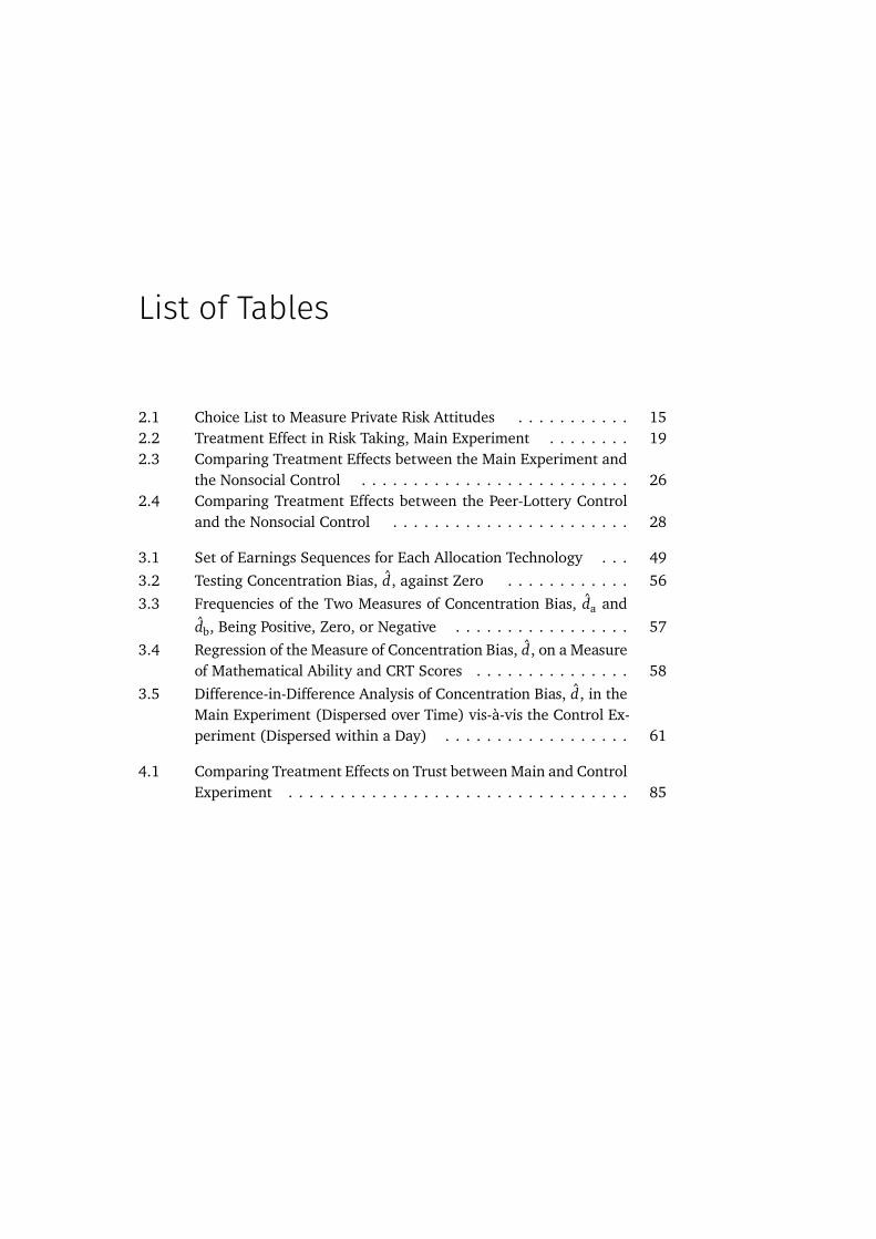
List of Tables
2.1 Choice List to Measure Private Risk Attitudes . . . . . . . . . . . 152.2 Treatment Effect in Risk Taking, Main Experiment . . . . . . . . 192.3 Comparing Treatment Effects between the Main Experiment and
the Nonsocial Control . . . . . . . . . . . . . . . . . . . . . . . . . . 262.4 Comparing Treatment Effects between the Peer-Lottery Control
and the Nonsocial Control . . . . . . . . . . . . . . . . . . . . . . . 28
3.1 Set of Earnings Sequences for Each Allocation Technology . . . 493.2 Testing Concentration Bias, d, against Zero . . . . . . . . . . . . 563.3 Frequencies of the Two Measures of Concentration Bias, da and
db, Being Positive, Zero, or Negative . . . . . . . . . . . . . . . . . 573.4 Regression of the Measure of Concentration Bias, d, on a Measure
of Mathematical Ability and CRT Scores . . . . . . . . . . . . . . . 583.5 Difference-in-Difference Analysis of Concentration Bias, d, in the
Main Experiment (Dispersed over Time) vis-à-vis the Control Ex-periment (Dispersed within a Day) . . . . . . . . . . . . . . . . . . 61
4.1 Comparing Treatment Effects on Trust betweenMain and ControlExperiment . . . . . . . . . . . . . . . . . . . . . . . . . . . . . . . . . 85

vi | List of Tables
1
Introduction?
Behavioral economics has improved the understanding of economic phenom-ena by enriching the understanding of economic decision making with insightsfrom psychology, sociology, and anthropology. Rigorous empirical investigationsof individual behavior—which commonly involve the use of laboratory experi-ments—have been at the heart of behavioral economics and have lead to newtheoretical accounts of decision making. The following three insights gave riseto influential branches of behavioral economics. First, the context in which indi-viduals make decisions often unleash behavioral influences that go beyond thoseidentified by standard economic theory. In particular, individual preferences com-monly depend on contextual features, as has been highlighted by the literatureson reference-dependent preferences (Kahneman and Tversky, 1979), and de-fault effects (Thaler and Sunstein, 2003). Second, individuals’ perception andprocessing of information often does not live up to the high demands of standardeconomic theory. Instead, individuals seem to employ simple heuristics (Tverskyand Kahneman, 1974) and attention-based decision rules (Kahneman, 2003) incomplex environments. Third, while standard economic theory typically con-strains individuals’ motives to pure self-interest, a more comprehensive view onindividuals’ behavior in social interactions uncovers that individuals often caredirectly about the well-being of others as well as about how they are viewed andtreated by others (Fehr and Falk, 2002).
This thesis consists of three chapters that each contribute to one of thesethree building blocks of research in behavioral economics.
In Chapter 2, I investigate the consequences of social reference points fordecision making under risk in a series of laboratory experiments. In the main ex-periment, decision makers observe the predetermined earnings of peer subjectsbefore making a risky choice. I exogenously manipulate peers’ earnings and finda significant treatment effect: decision makers make riskier choices in case of
? I would like to thank Holger Gerhardt for outstanding TeXnical assistance and numeroushelpful comments.
2 | 1 Introduction
larger peers’ earnings. The treatment effect is consistent with the predictions ofa model featuring social-comparison–based reference points and loss aversion.In two control experiments, I demonstrate that nonsocial—e.g., expectations-based—reference points do not explain the treatment effect.
In Chapter 3, I present novel results on individuals’ intertemporal choices injoint work with Holger Gerhardt and Louis Strang. Our findings cannot be ex-plained by exponential and hyperbolic discounting, the canonical approachesto intertemporal decision making in economics, but are consistent with anattention-based approach to intertemporal decision making that is based on con-centration bias. In particular, we provide causal evidence from novel lab exper-iments that intertemporal choices are systematically affected by whether con-sequences of intertemporal choice are concentrated in few or dispersed overmultiple periods: (i) Individuals are less patient in the case that the advantagesof patient behavior are dispersed over many future periods than when they areconcentrated in a single future period. (ii) Individuals are more patient in thecase that the disadvantages of patient behavior are dispersed over multiple ear-lier periods than when they are concentrated in a single earlier period. Bothfindings demonstrate concentration bias in individuals’ intertemporal choices.Our results are in line with the recent theoretical model of Kőszegi and Szeidl(2013). Despite the prevalence of dispersed payoffs and costs in everyday life, noempirical study so far has investigated whether spreading payments over timecausally impacts discounting. Our results suggest that previous studies may haveneglected an important channel that influences intertemporal decisions.
In Chapter 4, I study in joint work with Florian Zimmermann whether priorexperience of unfair versus fair treatment affects how much individuals trustothers? We provide causal evidence that trust is affected by prior personal expe-rience of fair versus unfair treatment by an unrelated third party. We comparethe willingness to trust of subjects in a lab experiment after they experiencedeither being paid or not being paid for a real-effort task by a peer subject. Af-ter being paid, subjects’ willingness to trust is substantially higher relative tosubjects who were not paid previously. Importantly, this treatment effect holdsdespite the fact that subjects knew the exact frequency with which subjects over-all got paid or did not get paid, such that the personal experience of fair versusunfair treatment did not provide additional information regarding the subse-quent interaction. Rational learning hence cannot explain the treatment effecton trust. By employing a control experiment, we show that the effect of expe-riencing fair versus unfair treatment on trust does also not result from incomeeffects: when subjects were paid based on a coin toss, subjects’ willingness totrust was similar to subjects who where not paid based on a coin toss.
References | 3
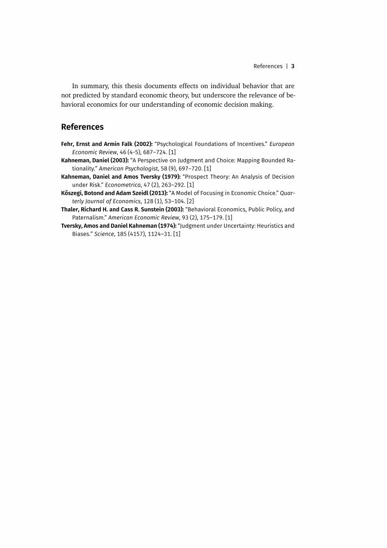
In summary, this thesis documents effects on individual behavior that arenot predicted by standard economic theory, but underscore the relevance of be-havioral economics for our understanding of economic decision making.
References
Fehr, Ernst and Armin Falk (2002): “Psychological Foundations of Incentives.” EuropeanEconomic Review, 46 (4-5), 687–724. [1]
Kahneman, Daniel (2003): “A Perspective on Judgment and Choice: Mapping Bounded Ra-tionality.” American Psychologist, 58 (9), 697–720. [1]
Kahneman, Daniel and Amos Tversky (1979): “Prospect Theory: An Analysis of Decisionunder Risk.” Econometrica, 47 (2), 263–292. [1]
Kőszegi, Botond and Adam Szeidl (2013): “A Model of Focusing in Economic Choice.” Quar-terly Journal of Economics, 128 (1), 53–104. [2]
Thaler, Richard H. and Cass R. Sunstein (2003): “Behavioral Economics, Public Policy, andPaternalism.” American Economic Review, 93 (2), 175–179. [1]
Tversky, Amos and Daniel Kahneman (1974): “Judgment under Uncertainty: Heuristics andBiases.” Science, 185 (4157), 1124–31. [1]

4 | 1 Introduction
2
Social Reference Pointsand Risk Taking?
2.1 Introduction
Since Kahneman and Tversky’s (1979) seminal prospect theory, the power-ful insights of reference-dependent preferences have enriched the toolbox ofeconomists in understanding individual behavior. The fundamental insight be-hind reference dependence is that individuals evaluate their obtained outcomesrelative to a reference point. Outcomes that are superior to the reference pointare perceived as gains, and inferior outcomes as losses. The essential feature ofreference-dependent preference models is loss aversion: Losses have a more pro-nounced negative effect on utility than equal-sized gains have a positive effect.
The key question in the literature on reference-dependent preferencesis: what determines the reference point? Behavioral predictions of reference-dependent preference models are highly sensitive to the specification of the ref-erence point, which constitute what individuals perceive as losses or gains. So far,reference points based on the status-quo and expected outcomes have been stud-
? I am deeply grateful to Steffen Altmann, Sebastian Kube, Matthias Wibral, Florian Zimmer-mann, and, especially, Armin Falk for their generous guidance and encouragement throughout thisproject. I thank Johannes Abeler, Mitra Akhtari, Alexander Cappelen, Stefano DellaVigna, ThomasDohmen, Sebastian Ebert, Benjamin Enke, Erik Eyster, Urs Fischbacher, Holger Gerhardt, LorenzGötte, Andreas Grunewald, Ori Heffetz, Simon Jäger, Andreas Kleiner, Botond Kőszegi, Ulrike Mal-mendier, Andrew Oswald, Gautam Rao, Paul Schempp, Andrei Shleifer, Dmitry Taubinsky, BertilTungodden, seminar participants at Bonn, Bergen, and Cologne, and conference participants atMünster, Madrid, Kreutzlingen, and Stockholm for their helpful comments. This research wasfinancially supported by the Bonn Graduate School of Economics and the Center for Economicsand Neuroscience in Bonn.
6 | 2 Social Reference Points and Risk Taking
ied predominantly within the literature. This improved both the understandingof reference-dependent preferences and of many economic phenomena.1
In this paper, I contribute to this vibrant literature by studying social-comparisons–based reference points. Surprisingly little attention has been paidto such social reference points within the literature on reference-dependent pref-erences.2 However, a rich tradition of research in psychology, sociology, anthro-pology, and the literature on social preferences in economics suggests that socialoutcomes are a reasonable source of the reference point. Not only do individualsfrequently engage in social comparisons (Festinger, 1954), but also individualwell-being often depends on social comparisons (e.g., Veblen, 1899; R. H. Frank,1985; Fliessbach et al., 2007; Card et al., 2012). Moreover, the perception ofunfair treatment commonly arises from comparisons to what others have (e.g.,Adams, 1963; Fehr and Schmidt, 1999; Bolton and Ockenfels, 2000; Falk andFischbacher, 2006).
The primary research questions of this study are (i) whether social referencepoints influence individual behavior when individuals’ decisions affect only theirown outcomes and (ii) whether loss aversion around social reference points ex-plains potential behavioral effects. By answering these questions, I contributeto the literature on social preferences. In form of inequity aversion, social–reference-point effects were studied in distributional games in which individ-uals were directly responsible for their peers’ earnings (e.g., Fehr and Schmidt,1999; Bolton and Ockenfels, 2000). It remains unclear whether these resultscan be generalized to decision making when individuals affect only their ownoutcomes. Distributional games constitute decision-making contexts where reci-procity (e.g., Levine, 1998; Falk and Fischbacher, 2006), welfare or efficiencyconcerns (e.g., Charness and Rabin, 2002; Engelmann and Strobel, 2004), andprosocial image concerns (e.g., Bénabou and Tirole, 2006; Ariely et al., 2009)may obfuscate social reference point effects on behavior.3 Importantly, reci-
1 These include, for instance, risk taking (e.g., Kahneman and Tversky, 1979; Rabin, 2000;Kőszegi and Rabin, 2007; Pope and Schweitzer, 2011; Sprenger, 2015), the premium equitypuzzle (e.g., Benartzi and Thaler, 1995; Gneezy and Potters, 1997; Kőszegi and Rabin, 2009),the disposition effect (e.g., Shefrin and Statman, 1985; Odean, 1998; Genesove andMayer, 2001),the endowment effect (e.g., Kahneman et al., 1990; Ericson and Fuster, 2011; Heffetz and List,2014), labor supply (e.g., Camerer et al., 1997; Kőszegi and Rabin, 2006; Crawford and Meng,2011), effort provision (e.g., Mas, 2006; Fehr and Goette, 2007; Abeler et al., 2011; Gill andProwse, 2012; Gneezy et al., 2013), price competition (Heidhues and Kőszegi, 2008), contractingin principal–agent settings (Herweg et al., 2010), soccer referees (Bartling et al., 2015), job search(DellaVigna et al., 2015), tax sheltering (Rees-Jones, 2014), and marathon running (Allen et al.,2014).
2 A notable exception is Linde and Sonnemans (2012), who tested whether prospect theory’sreflection effect extends to social reference points and found no evidence for it. In contrast toLinde and Sonnemans (2012), I study social–reference-point effects based on loss aversion.
3 For instance, giving in the dictator game and rejecting offers in the ultimatum game mayresult from an aversion against unequal outcomes. However, the former is also consistent withprosocial image concerns and the latter with reciprocating perceived unfair treatment.
2.1 Introduction | 7
procity, efficiency concerns, and prosocial image concerns do not predict social–reference-point effects on behavior when individuals affect only their own out-comes. By contrast, loss aversion around social reference points predicts behav-ioral effects.
I focus on decision making under risk to study social reference point effects.Risk taking is an important dimension of economic decision making (Dohmenet al., 2011). Understanding the determinants of risk taking is a fundamentalinterest of economic research. Additionally, the study of reference-dependentpreferences in economics emerged around empirical investigations of risk taking.
This paper employs a novel laboratory experiment that allows to providecausal evidence on whether social reference point affect risk taking and testsloss aversion around social reference points. In doing so, I address four criti-cal challenges. First, I induce social reference points to individuals who makea risky decision. Second, I exogenously vary the level of social reference pointsbetween two treatments, HI and LO. Third, decision-making subjects are ableto avoid earning less than their peer by making different risky choices betweenHI and LO treatments. Fourth, I employ two control experiments that allow totest alternative explanations based on nonsocial—e.g., expectations–based—reference points.
In each session of the main experiment, a single decision making subjectobserved the predetermined earnings, s, of a single peer subject before makinga risky choice. The risky choice allowed the decision maker to choose a binarylottery from a set of lotteries. Essentially, decision makers chose an upside pay-ment between €3 and €16.5. The larger the decision maker chose this upside tobe, the lower was the likelihood of receiving it. The downside of each lottery wasno payment. Subjects could choose riskier lotteries—combining larger upsideswith lower likelihoods of receiving them—or less risky lotteries—combininglower upsides with higher upside likelihoods. Ultimately, this choice involved atrade-off between the size of the upside and its likelihood.
In a between-subject design, I varied the predetermined earnings of the peerbetween sHI = €8 (HI treatment) and sLO = €2 (LO). Since there were only 2subjects—one decision maker and one peer—present in the lab per experimen-tal session, peers’ earnings served as a natural comparison standard. In thatsense the design allowed me to induce relevant social reference points to therisk-taking subjects. Additionally, decision makers knew that their outcomes andrisky choices would never be revealed to their peers.
To derive predictions, I formalize the impact of peer earnings on risk tak-ing in a simple model featuring social-comparisons–based reference points andloss aversion. In the case that individual behavior follows expected utility the-ory, no treatment effect on risk taking is expected, since decision makers facethe same risky choice across treatments. In the case that individuals evaluate

8 | 2 Social Reference Points and Risk Taking
lottery outcomes according to loss aversion around their peers’ earnings, thetreatment manipulation changes their risk-taking incentives: decision makerschoose larger upsides, i.e., riskier lotteries, in HI than in LO to avoid earningless than their peer.
This is precisely what happened in the experiment: Decision makers chosean average upside of €8.25 when their peers’ earnings were €8; and they chosean average upside of €7 when their peers’ earnings were €2. This treatmenteffect on risk taking is statistically significant and provides affirmative evidencethat social reference points affect risk taking.
However, an alternative explanation behind the treatment effect on risk tak-ing may be loss aversion relative to expectations–based reference points—ratherthan social reference points. Before decisionmakers knew their risky choice, theyonly knew what they could have earned, if they had been assigned to the peerrole. These counterfactual earnings informed their expectations regarding theirown earnings, leading to potential differences in expectations–based referencepoints between HI-LO treatments before decision makers were informed abouttheir risky choices.
Based on Kőszegi and Rabin (2006, 2007), expectations–based referencepoints can, but do not have to, account for the treatment effect on risk taking.Considering the timing of the experiment, the critical question for expectations–based reference points is whether decision makers change expectations–basedreference points quickly in light of new information or slowly. If expectations–based reference points changed quickly after decision makers were introducedto their risky choices, then no treatment effect would be predicted. This fol-lows from the fact that the risky choices are constant across the HI and theLO treatment. However, the treatment effect on risk taking is consistent withexpectations–based reference points that do not (sufficiently) change after deci-sion makers are introduced to their risky choice.
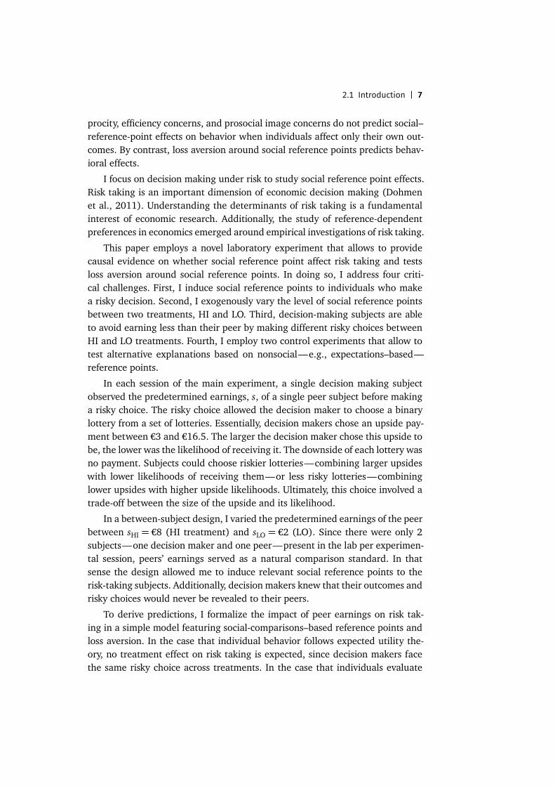
By comparing risk taking between the main experiment and two controlexperiments that are discussed in detail below, I investigate whether the treat-ment effect on risk taking is caused by social reference points (SRPs) or whetherit could also result from slowly changing expectations–based reference points(ERPs). In the nonsocial control, SRPs predict no treatment effect on risk tak-ing and ERPs make the same predictions as for the main experiment. The peer-lottery control experiment is designed to reverse these predictions. ERPs predictno treatment effect on risk taking, while SRP predict a similar treatment effectcompared to the main experiment. Overall, the results are in favour of SRPs asthe driver of risk taking in all experiments: There is no treatment effect on risktaking in the nonsocial control while there is a treatment effect on risk takingin the peer-lottery control. Figure 2.1 provides an overview of how the control
2.1 Introduction | 9
Main
Procedure: 2 subjects cointoss
decisionmaker:
peer: receives s
observesreceives
risky choiceperforms
risky choice
Treatments: s = €8 in HI and s = €2 in LO
Conducted: in fall 2012, spring 2013, and fall 2014
Nonsocial
Procedure: 1 subject cointoss
active:
passive: receives r
observesreceives
risky choiceperforms
risky choice
Treatments: r = €8 in HI and r = €2 in LO
Conducted: in spring 2013, summer 2014, and fall 2014
Peer-Lottery
Procedure: 2 subjects cointoss
decisionmaker:
peer:lottery:
€8 or €2
delay
of 5minreceives s
observesreceives
risky choiceperforms
risky choice
Treatments: s = €8 in HI and s = €2 in LO
Conducted: in summer 2014
Figure 2.1. Overview of all Risk-Taking Experiments
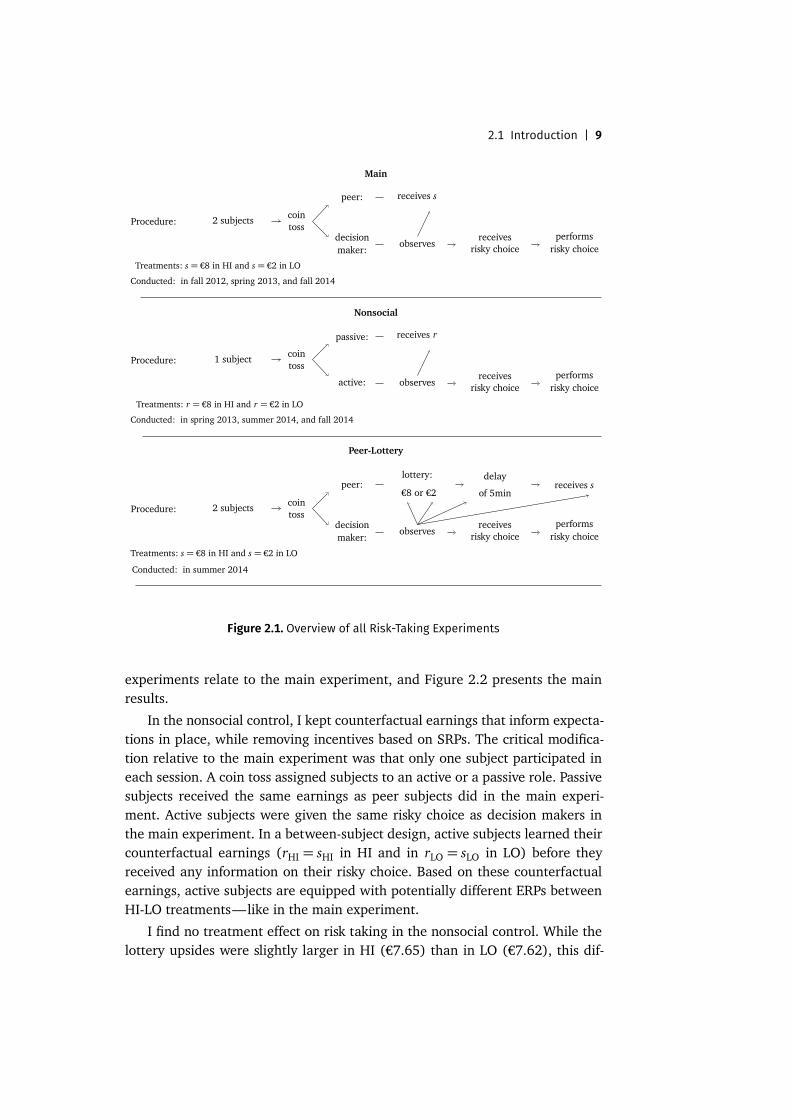
experiments relate to the main experiment, and Figure 2.2 presents the mainresults.
In the nonsocial control, I kept counterfactual earnings that inform expecta-tions in place, while removing incentives based on SRPs. The critical modifica-tion relative to the main experiment was that only one subject participated ineach session. A coin toss assigned subjects to an active or a passive role. Passivesubjects received the same earnings as peer subjects did in the main experi-ment. Active subjects were given the same risky choice as decision makers inthe main experiment. In a between-subject design, active subjects learned theircounterfactual earnings (rHI = sHI in HI and in rLO = sLO in LO) before theyreceived any information on their risky choice. Based on these counterfactualearnings, active subjects are equipped with potentially different ERPs betweenHI-LO treatments—like in the main experiment.
I find no treatment effect on risk taking in the nonsocial control. While thelottery upsides were slightly larger in HI (€7.65) than in LO (€7.62), this dif-
10 | 2 Social Reference Points and Risk Taking
67
89
10Up
side
of th
e Pr
efer
red
Lotte
ry
Main (N = 132) Nonsocial (N = 134) Peer−lottery (N = 131)
HI Treatments LO Treatments
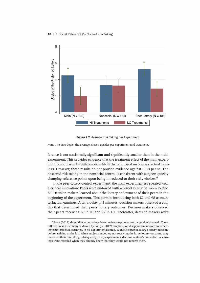
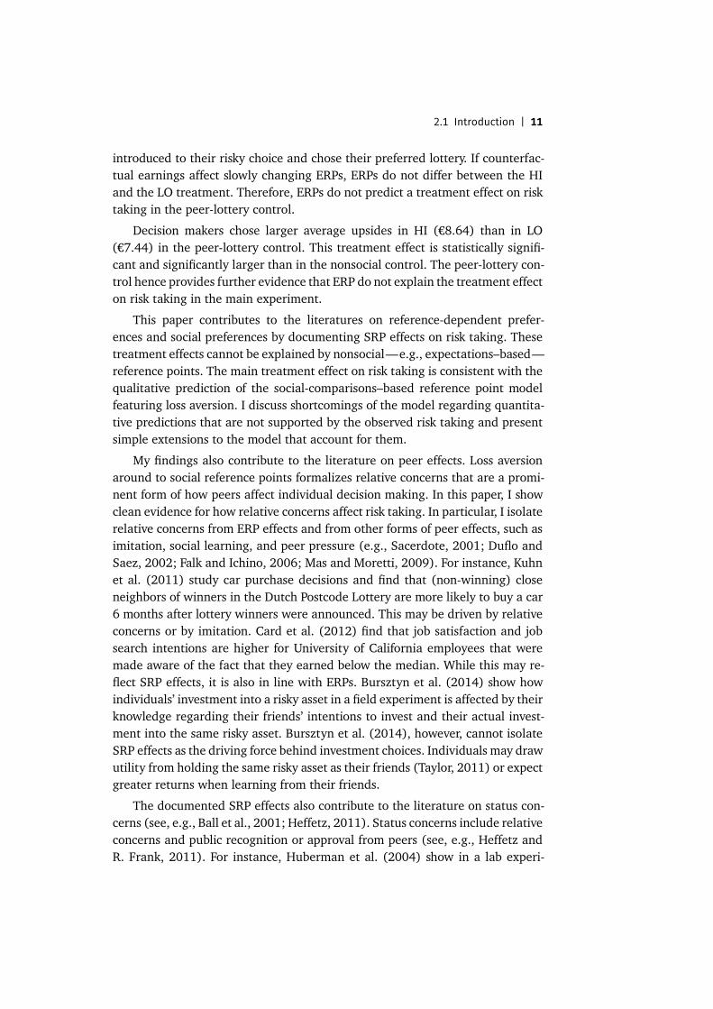
Figure 2.2. Average Risk Taking per Experiment
Note: The bars depict the average chosen upsides per experiment and treatment.
ference is not statistically significant and significantly smaller than in the mainexperiment. This provides evidence that the treatment effect of the main experi-ment is not driven by differences in ERPs that are based on counterfactual earn-ings. However, these results do not provide evidence against ERPs per se. Theobserved risk taking in the nonsocial control is consistent with subjects quicklychanging reference points upon being introduced to their risky choices.4
In the peer-lottery control experiment, the main experiment is repeated witha critical innovation: Peers were endowed with a 50-50 lottery between €2 and€8. Decision makers learned about the lottery endowment of their peers in thebeginning of the experiment. This permits introducing both €2 and €8 as coun-terfactual earnings. After a delay of 5 minutes, decision makers observed a coinflip that determined their peers’ lottery outcomes. Decision makers observedtheir peers receiving €8 in HI and €2 in LO. Thereafter, decision makers were
4 Song (2012) shows that expectations-based reference points can change slowly as well. Thesedifferent results seem to be driven by Song’s (2012) emphasis on disappointment over not receiv-ing counterfactual earnings. In his experimental setup, subjects expected a large lottery outcomebefore arriving at the lab. When subjects ended up not receiving the large lottery outcome, theyincreased their risk taking subsequently. In my experiments, decision makers’ counterfactual earn-ings were revealed when they already knew that they would not receive them.
2.1 Introduction | 11
introduced to their risky choice and chose their preferred lottery. If counterfac-tual earnings affect slowly changing ERPs, ERPs do not differ between the HIand the LO treatment. Therefore, ERPs do not predict a treatment effect on risktaking in the peer-lottery control.
Decision makers chose larger average upsides in HI (€8.64) than in LO(€7.44) in the peer-lottery control. This treatment effect is statistically signifi-cant and significantly larger than in the nonsocial control. The peer-lottery con-trol hence provides further evidence that ERP do not explain the treatment effecton risk taking in the main experiment.
This paper contributes to the literatures on reference-dependent prefer-ences and social preferences by documenting SRP effects on risk taking. Thesetreatment effects cannot be explained by nonsocial—e.g., expectations–based—reference points. The main treatment effect on risk taking is consistent with thequalitative prediction of the social-comparisons–based reference point modelfeaturing loss aversion. I discuss shortcomings of the model regarding quantita-tive predictions that are not supported by the observed risk taking and presentsimple extensions to the model that account for them.
My findings also contribute to the literature on peer effects. Loss aversionaround to social reference points formalizes relative concerns that are a promi-nent form of how peers affect individual decision making. In this paper, I showclean evidence for how relative concerns affect risk taking. In particular, I isolaterelative concerns from ERP effects and from other forms of peer effects, such asimitation, social learning, and peer pressure (e.g., Sacerdote, 2001; Duflo andSaez, 2002; Falk and Ichino, 2006; Mas and Moretti, 2009). For instance, Kuhnet al. (2011) study car purchase decisions and find that (non-winning) closeneighbors of winners in the Dutch Postcode Lottery are more likely to buy a car6 months after lottery winners were announced. This may be driven by relativeconcerns or by imitation. Card et al. (2012) find that job satisfaction and jobsearch intentions are higher for University of California employees that weremade aware of the fact that they earned below the median. While this may re-flect SRP effects, it is also in line with ERPs. Bursztyn et al. (2014) show howindividuals’ investment into a risky asset in a field experiment is affected by theirknowledge regarding their friends’ intentions to invest and their actual invest-ment into the same risky asset. Bursztyn et al. (2014), however, cannot isolateSRP effects as the driving force behind investment choices. Individuals may drawutility from holding the same risky asset as their friends (Taylor, 2011) or expectgreater returns when learning from their friends.
The documented SRP effects also contribute to the literature on status con-cerns (see, e.g., Ball et al., 2001; Heffetz, 2011). Status concerns include relativeconcerns and public recognition or approval from peers (see, e.g., Heffetz andR. Frank, 2011). For instance, Huberman et al. (2004) show in a lab experi-
12 | 2 Social Reference Points and Risk Taking
ment that subjects forwent material gains in order to win a contest that wastied to a public victory announcement. My findings complement these findingsby showing that relative concerns matter independently of public recognition bypeers.
I proceed in Section 2.2 with providing evidence for social reference pointeffects. I establish that these social reference point effects cannot be explainedby expectations–based reference points in Section 2.3. Section 2.4 concludes.
2.2 Evidence for Social Reference Point Effects
This section provides evidence that social reference points affect individual risktaking. In the following I present the design of the main experiment and derivebehavioral predictions from a social-comparisons–based reference point model.Then I report and discuss the findings of the experiment.
2.2.1 Main Experiment
The main experiment is designed to allow for a precise measurement of risktaking after decision makers have been made aware of the earnings of their peersubjects. Between two treatments, I exogenously manipulate the predeterminedpeer earnings. A between-subject comparison of risk taking across treatmentsallows identifying the effect of social reference points.
Two subjects participated in each lab session. Upon subjects’ arrival, the ex-perimenter tossed a coin in front of their eyes to assign them to one of two roles:decision maker and peer (called participant A and B in the experiment). There-after, subjects received role-specific instructions in private.5 Peers learned thatthey would receive a show-up fee and an additional payment of €s for complet-ing a survey. Thereafter, they completed the survey and left the lab once theywere done. Decision makers, first, learned that they would receive a show-up feeand that they could earn an additional payment for completing the same surveytheir peers had to complete. Before receiving any information on their own ad-ditional payment, they learned the show-up fee and additional payment of theirpeers. Second, decision makers were told that their own additional paymentwas not predetermined, but the outcome of a risky choice. Third, they learnedthat their peers received no information on their behalf and would leave the labearlier than they would. Fourth, they were introduced to their risky choice. Fifth,they performed their risky choice. Finally, decision makers completed the surveyand left the lab once they were done—which was by design 5–10 minutes aftertheir peers.
5 Appendix 4.A provides a translation of the instructions.
2.2 Evidence for Social Reference Point Effects | 13
x
EV Var
16.58.25
5.04
12.67
32.62
3
EV Var
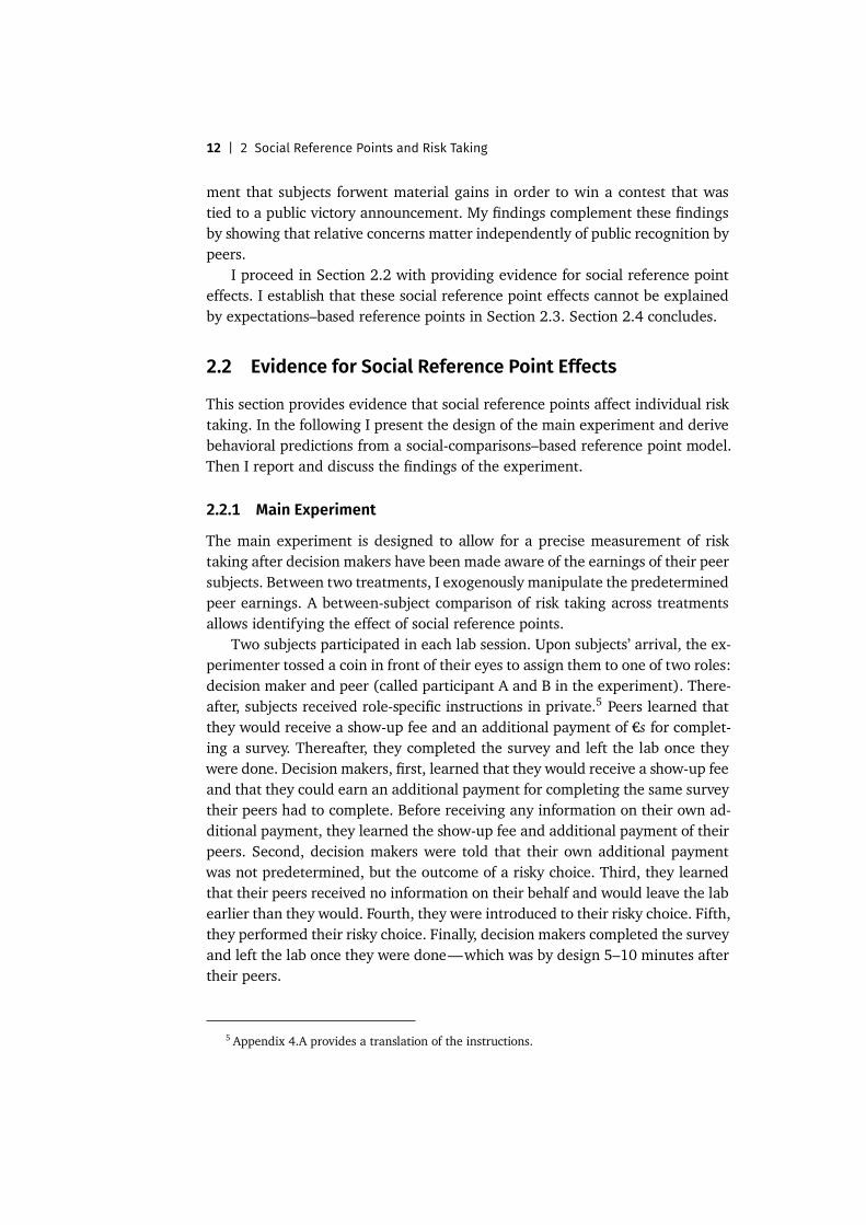
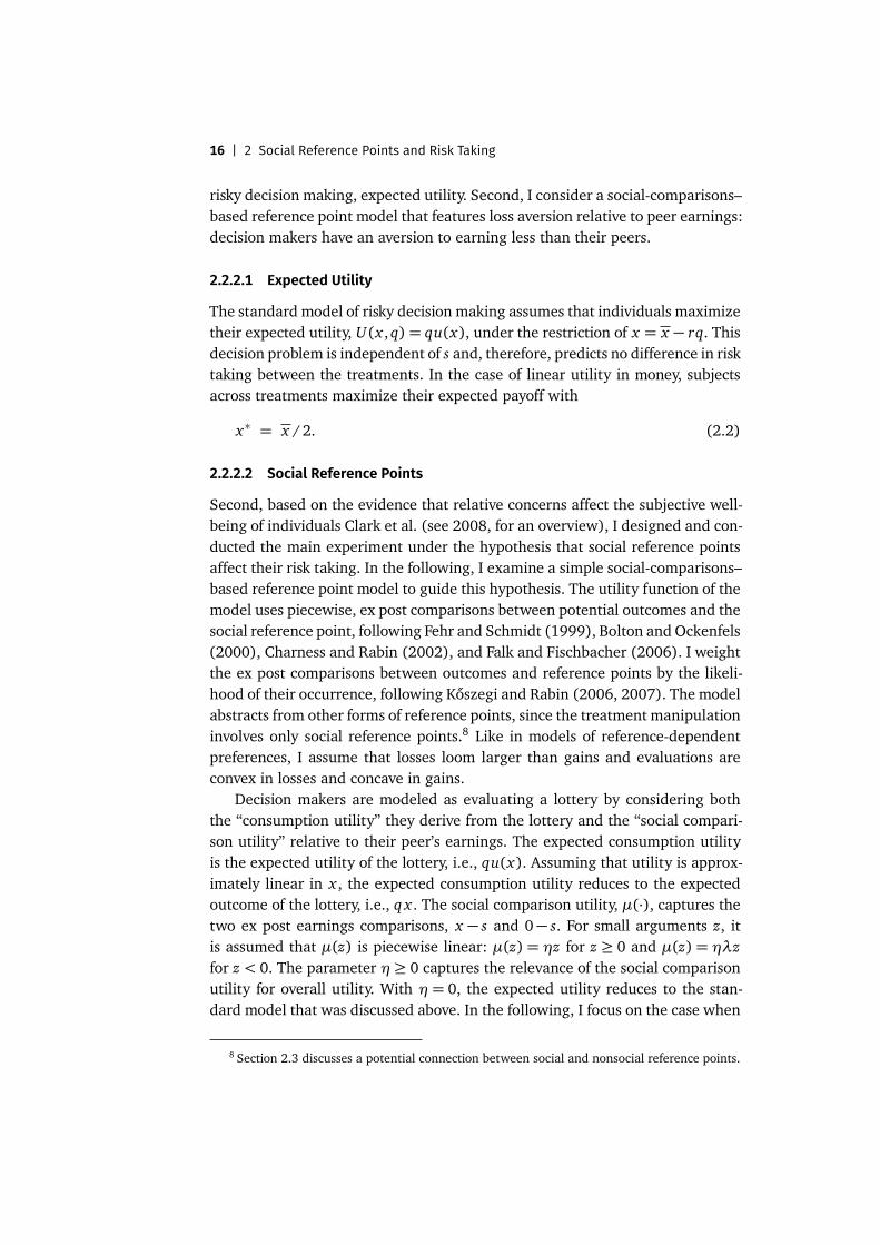
Figure 2.3. Properties of the Lotteries
Note: The solid graph shows how the expected value of all lotteries varies in the lotteries’ upside,x . The dotted graph shows how the variance varies in x .
All decision makers faced the same risky choice which is based on An-dreoni and Harbaugh (2010). Decision makers chose their preferred binarylottery (x(q), q) from a set of lotteries. Each lottery paid an upside ofx(q)= €16.5− €13.5q with an upside likelihood of q = i /100, for integersi ∈ [0,100], and nothing instead. Thus, the set of lotteries entailed, e.g., a cer-tain payment of €3, (€3, 100%), an upside of €9.75 with an upside likelihoodof 50%, (€9.75, 50%), and an upside of €16.23 with an upside likelihood of 2%,(€16.23, 2%). Decision makers chould choose riskier lotteries—that combinedlarger upsides with lower upside likelihoods—or less risky lotteries—that com-bined lower upsides with higher upside likelihoods. Figure 2.3 depicts what thisrelationship implies for the expected value and variance of these lotteries. Ul-timately, decision makers faced a mean-variance trade-off for lotteries with anupside below €8.25.
I used a visual elicitationmethod that made it easy for subjects to understandthe lottery choice. Appendix 2.B provides screenshots of the decision screens.
In the HI treatment, decision makers chose their preferred lottery after learn-ing that their peer received sHI = €8. The construction of the risky choice gavethem a chance to earn more (or not to earn less) than their peers. In the LOtreatment, decision makers’ peers received sLO = €2. The risky choice alloweddecision makers to choose a lottery that combined a higher upside likelihoodwith a lower upside. This enabled them to avoid falling behind the peer.
The only variation between the two treatments was the level of the peerearnings. Hence, a difference in the decision makers’ risk taking between thetreatments allows identifying the impact of social reference points. Our designrules out the influence of other peer effects—e.g., imitation, learning, or socialpressure: decision makers did not observe actions of any other subjects; deci-
14 | 2 Social Reference Points and Risk Taking
sion makers did not affect peer outcomes; and decision makers knew that theirchoices and outcomes were not revealed to others.6
2.2.1.1 Private Risk Attitudes
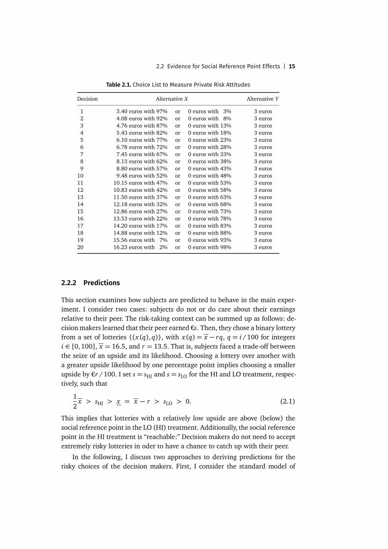
Between one and two weeks after the main experiment, decision makers re-turned to the lab and received €8 as a show-up fee. In this second part, I elicitedtheir private risk attitudes, i.e., their individual risk attitudes in the absence ofany peer effects. I use this as a control variable in the analysis of the risk-takingbehavior in the main experiment. Each decision maker faced 20 price-list–styleddecisions. Each decision was a choice between Alternative Y , a certain amount ofmoney, and Alternative X , a binary lottery. Alternative Y was always €3. Alterna-tive X was a distinct lottery for each decision. Along the 20 decisions, AlternativeX is getting more risky. Subjects started choosing Alternative X and switched toAlternative Y at some point. I interpret this switching point as a proxy of thedecision makers’ risk attitudes. I classify them as more (less) risk-averse, theearlier (later) they switched.7 Table 2.1 lists all 20 decisions.
2.2.1.2 Procedure
The main experiment was conducted in three waves at two office rooms of theBonn Graduate School of Economics in fall 2012 and spring 2013 and of the Bon-nEconLab in fall 2014. By using two rooms, both treatments, HI and LO, wereconducted simultaneously. In total, 264 subjects—132 decision makers and 132peers—participated in 132 sessions of the main experiment. No subject partici-pated in more than one treatment (and in any other experiment conducted forthis paper). I invited only male subjects to keep the sample homogenous. Eachsession lasted for 12 to 20 minutes. Subjects earned on average €8.5. The secondpart of the experiment was conducted at the BonnEconLab. All but 6 decisionmakers from the main experiment participated (attrition rate of 5%). Each ses-sion lasted for 10 to 40 minutes. Subjects earned on average €12.7. All experi-ments in this paper were computerized using the softwares z-Tree (Fischbacher,2007) and ORSEE (Greiner, 2004).
6 In case pairs of decision maker and peer subjects knew each other, decision makers may haveanticipated talking to their peers about the experiment afterwards. Therefore, all decision makersand peers were asked whether they had known each other prior to the experiment—which wastrue for 5 pairs. All results presented in this paper remain virtually unchanged when focusingonly on pairs of strangers.
7 This price-list elicitation method allows subjects to switch multiple times. For subjects whoswitched multiple times, the mean switching point is used to proxy their risk attitude.
2.2 Evidence for Social Reference Point Effects | 15
Table 2.1. Choice List to Measure Private Risk Attitudes
Decision Alternative X Alternative Y
1 3.40 euros with 97% or 0 euros with 3% 3 euros2 4.08 euros with 92% or 0 euros with 8% 3 euros3 4.76 euros with 87% or 0 euros with 13% 3 euros4 5.43 euros with 82% or 0 euros with 18% 3 euros5 6.10 euros with 77% or 0 euros with 23% 3 euros6 6.78 euros with 72% or 0 euros with 28% 3 euros7 7.45 euros with 67% or 0 euros with 33% 3 euros8 8.13 euros with 62% or 0 euros with 38% 3 euros9 8.80 euros with 57% or 0 euros with 43% 3 euros
10 9.48 euros with 52% or 0 euros with 48% 3 euros11 10.15 euros with 47% or 0 euros with 53% 3 euros12 10.83 euros with 42% or 0 euros with 58% 3 euros13 11.50 euros with 37% or 0 euros with 63% 3 euros14 12.18 euros with 32% or 0 euros with 68% 3 euros15 12.86 euros with 27% or 0 euros with 73% 3 euros16 13.53 euros with 22% or 0 euros with 78% 3 euros17 14.20 euros with 17% or 0 euros with 83% 3 euros18 14.88 euros with 12% or 0 euros with 88% 3 euros19 15.56 euros with 7% or 0 euros with 93% 3 euros20 16.23 euros with 2% or 0 euros with 98% 3 euros
2.2.2 Predictions
This section examines how subjects are predicted to behave in the main exper-iment. I consider two cases: subjects do not or do care about their earningsrelative to their peer. The risk-taking context can be summed up as follows: de-cisionmakers learned that their peer earned €s. Then, they chose a binary lotteryfrom a set of lotteries {(x(q), q)}, with x(q)= x − rq, q = i /100 for integersi ∈ [0,100], x = 16.5, and r = 13.5. That is, subjects faced a trade-off betweenthe seize of an upside and its likelihood. Choosing a lottery over another witha greater upside likelihood by one percentage point implies choosing a smallerupside by €r /100. I set s = sHI and s = sLO for the HI and LO treatment, respec-tively, such that
12
x > sHI > x = x − r > sLO > 0. (2.1)
This implies that lotteries with a relatively low upside are above (below) thesocial reference point in the LO (HI) treatment. Additionally, the social referencepoint in the HI treatment is “reachable:” Decision makers do not need to acceptextremely risky lotteries in oder to have a chance to catch up with their peer.
In the following, I discuss two approaches to deriving predictions for therisky choices of the decision makers. First, I consider the standard model of
16 | 2 Social Reference Points and Risk Taking
risky decision making, expected utility. Second, I consider a social-comparisons–based reference point model that features loss aversion relative to peer earnings:decision makers have an aversion to earning less than their peers.
2.2.2.1 Expected Utility
The standard model of risky decision making assumes that individuals maximizetheir expected utility, U(x , q)= qu(x), under the restriction of x = x − rq. Thisdecision problem is independent of s and, therefore, predicts no difference in risktaking between the treatments. In the case of linear utility in money, subjectsacross treatments maximize their expected payoff with
x∗ = x /2. (2.2)
2.2.2.2 Social Reference Points
Second, based on the evidence that relative concerns affect the subjective well-being of individuals Clark et al. (see 2008, for an overview), I designed and con-ducted the main experiment under the hypothesis that social reference pointsaffect their risk taking. In the following, I examine a simple social-comparisons–based reference point model to guide this hypothesis. The utility function of themodel uses piecewise, ex post comparisons between potential outcomes and thesocial reference point, following Fehr and Schmidt (1999), Bolton and Ockenfels(2000), Charness and Rabin (2002), and Falk and Fischbacher (2006). I weightthe ex post comparisons between outcomes and reference points by the likeli-hood of their occurrence, following Kőszegi and Rabin (2006, 2007). The modelabstracts from other forms of reference points, since the treatment manipulationinvolves only social reference points.8 Like in models of reference-dependentpreferences, I assume that losses loom larger than gains and evaluations areconvex in losses and concave in gains.
Decision makers are modeled as evaluating a lottery by considering boththe “consumption utility” they derive from the lottery and the “social compari-son utility” relative to their peer’s earnings. The expected consumption utilityis the expected utility of the lottery, i.e., qu(x). Assuming that utility is approx-imately linear in x , the expected consumption utility reduces to the expectedoutcome of the lottery, i.e., q x . The social comparison utility, µ(·), captures thetwo ex post earnings comparisons, x − s and 0− s. For small arguments z, itis assumed that µ(z) is piecewise linear: µ(z)= ηz for z ≥ 0 and µ(z)= ηλzfor z < 0. The parameter η≥ 0 captures the relevance of the social comparisonutility for overall utility. With η= 0, the expected utility reduces to the stan-dard model that was discussed above. In the following, I focus on the case when
8 Section 2.3 discusses a potential connection between social and nonsocial reference points.

2.2 Evidence for Social Reference Point Effects | 17
social comparison utility is relevant for decisions, i.e., η > 0. The parameter λcaptures how individuals evaluate having less than others. For λ > 1, individualsare loss-averse.
The expected utility of choosing a lottery with x > s is
U(x , q(x) | s) = q(x)x + q(x)η(x − s) + (1 − q(x))ηλ(0 − s). (2.3)
The first term on the right-hand side is the expected consumption utility of thelottery. The second and third terms are, respectively, the expected social gainand social loss.
For lotteries with x < s, the expected social comparison utility collapses tolosses only,
U(x , q(x) | s) = q(x)x + q(x)ηλ(x − s) − (1 − q(x))ηλs. (2.4)
Consider first the LO treatment. Because decision makers can only chooselotteries with an upside above their peer’s earnings, i.e., x > sLO, they maximizetheir expected utility of equation (2.3) under the restriction of x = x − rq, yield-ing
∂ U(x | sLO)∂ x
!= 0 ⇐⇒ x∗LO = x∗ + ψ∗sLO,
with ψ∗ =η(1 − λ)2(1 + η)
< 0.
Compared to the standard model of risky choice (with η= 0), loss aversion in-duces decision makers to choose a less risky lottery, i.e., a lower upside. By de-creasing x , decision makers increase their chances of “securing” an outcomeabove sLO.
In the HI treatment, decision makers can choose lotteries with upsides aboveand below their peer’s earnings, since x > sHI > x . Their marginal utility of tak-ing risk is:
∂ U(x | sHI)∂ x
¨
< 0 if x > sHI> 0 if x < sHI.
(2.5)
First, assume decision makers contemplate choosing an upside that exceeds theearnings of their peer, x > sHI. Equation (2.5) states that the marginal utilityof taking risk is negative: for any value of x above sHI, decision makers preferto reduce their risk taking—choose a smaller x—in order to avoid earningsless than the peer up to the point that x = sHI. In the case that decision makersconsider a lottery with x < sHI, the marginal utility of taking risk is positive,equation (2.5). This reflects the following: if decision makers choose a lotterythat leaves them in an unfavorable relative position, they revert to choosing the
18 | 2 Social Reference Points and Risk Taking
lottery with the maximum expected value. However, the lottery with maximumexpected value has an upside larger than the earnings of his peer. Therefore,loss-averse decision makers settle at setting x∗HI = sHI. They modify their riskybehavior to match ex post earnings between their peer and themselves for thecase of receiving the lottery’s upside.
The model predicts that sufficiently loss-averse decision makers chooseriskier lotteries in the HI than in the LO treatment, i.e., x∗LO < x∗HI.
9 In the LOtreatment, loss aversion induces decision makers to reduce their risk taking inorder to secure their favorable relative earnings and avoid falling behind theirpeer from too much risk taking. In the HI treatment, decision makers chooseriskier lotteries to be able to “catch up” with their peer by matching their up-side with their peer’s earnings. Based on this argument, my main qualitativehypothesis is:
Hypothesis 1. Loss-averse decision makers choose lotteries with larger upsides inHI than in LO, i.e., xLO < xHI.
Based on the discussing of how loss-averse subjects in the HI treatment be-have, I also make a quantitative prediction:
Hypothesis 2. Loss-averse decision makers bunch at the lottery with an upside of€8 in HI, i.e., xHI = sHI.
From Hypotheses 1 and 2 follows also the prediction that decision makerschoose lotteries with a larger expected value in HI than in LO. Loss-averse sub-jects bunch around the lottery with the €8 upside in HI, which is close to theupside of the lottery with the highest expected value, and choose lower upsidesin LO.
Hypothesis 3. Loss-averse subjects choose, on average, a lottery with a higherexpected value in HI than in LO.
2.2.3 Results of the Main Experiment
The first result supports Hypothesis 1. In the LO treatment with peer earningsof €2, decision makers chose an average upside of €7. In the HI treatment withpeer earnings of €8, the preferred lottery of decision makers paid an averageupside of €8.25.
Comparing LO to HI, decision makers reduced their risk taking by decreasingtheir average upside by €1.25—a marginal effect of 18%. The mean differencein upsides between treatments is significant in an OLS regression. Column 1of Table 2.2 shows the results of regressing the upside choices of each decision
9 Sufficient loss aversion is λ > 1+µ, with µ= ((x − 2sHI) / sLO)((1+η) /η). For instance, ifη= 1, then µ= 1/2 and λ > 3/2.
2.2 Evidence for Social Reference Point Effects | 19
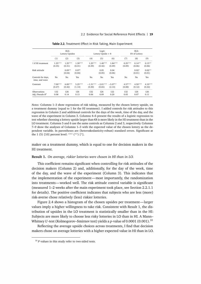
Table 2.2. Treatment Effect in Risk Taking, Main Experiment
OLS: Logit: OLS:Lottery Upsides Lottery Upside > 8 EV of Lottery
(1) (2) (3) (4) (5) (6) (7) (8) (9)
1 if HI treatment 1.25*** 1.25*** 1.30*** 1.25*** 1.40*** 1.84*** 0.25*** 0.14** 0.15**(0.35) (0.31) (0.31) (0.39) (0.42) (0.49) (0.09) (0.06) (0.06)
Risk attitude 0.09** 0.07* 0.05 0.04 0.02* 0.02**(0.04) (0.04) (0.05) (0.06) (0.01) (0.01)
Controls for days, No No Yes No No Yes No No Yestime, and wave
Constant 7.00*** 6.00*** 5.25*** −1.31*** −2.01*** −5.07** 4.57*** 4.50*** 4.10***(0.27) (0.42) (1.14) (0.30) (0.65) (2.14) (0.08) (0.12) (0.32)
Observations 132 126 126 132 126 122 132 126 126Adj./Pseudo R2 0.08 0.14 0.13 0.06 0.09 0.20 0.05 0.07 0.11
Notes: Columns 1–3 show regressions of risk taking, measured by the chosen lottery upside, ona treatment dummy (equal to 1 for the HI treatment). I added controls for risk attitudes to thisregression in Column 2 and additional controls for the days of the week, time of the day, and thewave of the experiment in Column 3. Columns 4–6 present the results of a logistic regression totest whether choosing a lottery upside larger than €8 is more likely in the HI treatment than in theLO treatment. Columns 5 and 6 use the same controls as Columns 2 and 3, respectively. Columns7–9 show the analyses of Columns 1–3 with the expected value of the chosen lottery as the de-pendent variable. In parentheses are (heteroskedasticity-robust) standard errors. Significant atthe 1 (5) [10] percent level: *** (**) [*].
maker on a treatment dummy, which is equal to one for decision makers in theHI treatment.
Result 1. On average, riskier lotteries were chosen in HI than in LO.
This coefficient remains significant when controlling for risk attitudes of thedecision makers (Column 2) and, additionally, for the day of the week, timeof the day, and the wave of the experiment (Column 3). This indicates thatthe implementation of the experiment—most importantly, the randomizationinto treatments—worked well. The risk attitude control variable is significant(measured 1–2 weeks after the main experiment took place, see Section 2.2.1.1for details). The positive coefficient indicates that subjects who are less (more)risk-averse chose relatively (less) riskier lotteries.
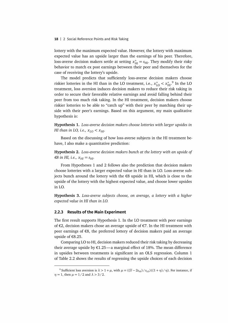
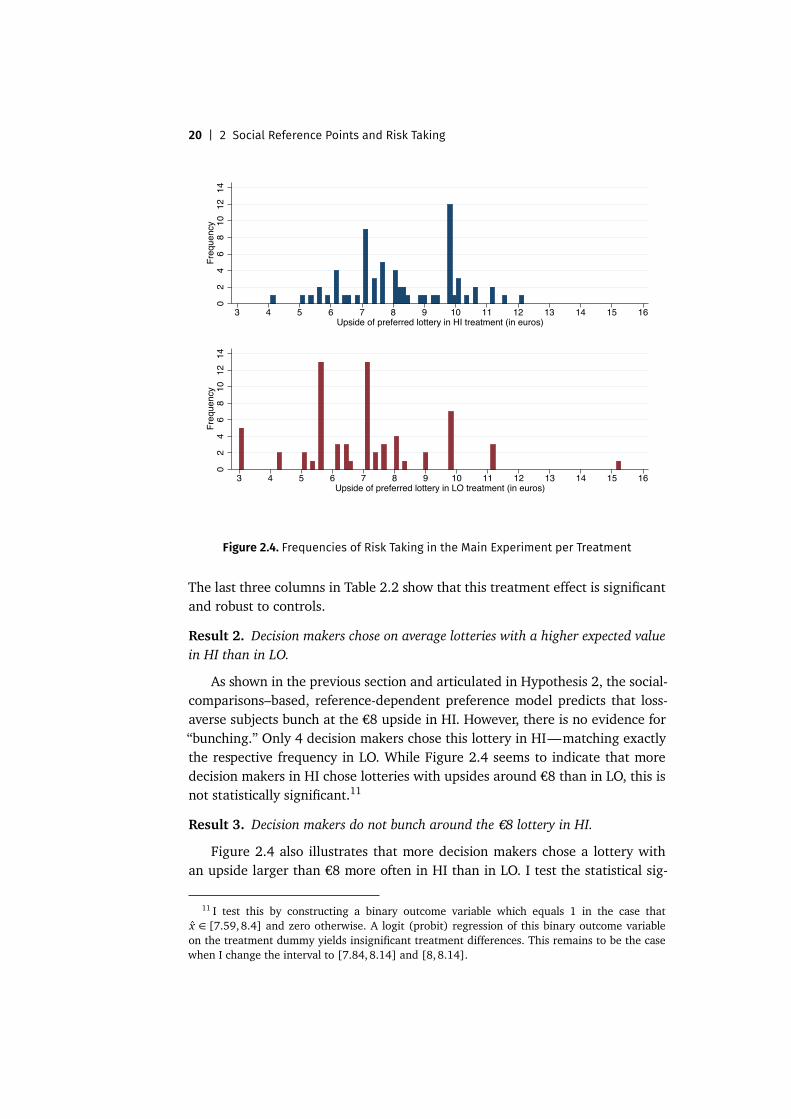
Figure 2.4 shows a histogram of the chosen upsides per treatment—largervalues imply a higher willingness to take risk. Consistent with Result 1, the dis-tribution of upsides in the LO treatment is statistically smaller than in the HI:Subjects are more likely to choose less risky lotteries in LO than in HI. A Mann–Whitney U-test (Kolmogorov–Smirnov test) yields a p-value of 0.0001 (0.001).10
Reflecting the average upside choices across treatments, I find that decisionmakers chose on average lotteries with a higher expected value in HI than in LO.
10 P-values in this study refer to two-sided tests.
20 | 2 Social Reference Points and Risk Taking
02
46
810
1214
Freq
uenc
y
3 4 5 6 7 8 9 10 11 12 13 14 15 16Upside of preferred lottery in HI treatment (in euros)
02
46
810
1214
Freq
uenc
y
3 4 5 6 7 8 9 10 11 12 13 14 15 16Upside of preferred lottery in LO treatment (in euros)
Figure 2.4. Frequencies of Risk Taking in the Main Experiment per Treatment
The last three columns in Table 2.2 show that this treatment effect is significantand robust to controls.
Result 2. Decision makers chose on average lotteries with a higher expected valuein HI than in LO.
As shown in the previous section and articulated in Hypothesis 2, the social-comparisons–based, reference-dependent preference model predicts that loss-averse subjects bunch at the €8 upside in HI. However, there is no evidence for“bunching.” Only 4 decision makers chose this lottery in HI—matching exactlythe respective frequency in LO. While Figure 2.4 seems to indicate that moredecision makers in HI chose lotteries with upsides around €8 than in LO, this isnot statistically significant.11
Result 3. Decision makers do not bunch around the €8 lottery in HI.
Figure 2.4 also illustrates that more decision makers chose a lottery withan upside larger than €8 more often in HI than in LO. I test the statistical sig-
11 I test this by constructing a binary outcome variable which equals 1 in the case thatx ∈ [7.59, 8.4] and zero otherwise. A logit (probit) regression of this binary outcome variableon the treatment dummy yields insignificant treatment differences. This remains to be the casewhen I change the interval to [7.84,8.14] and [8, 8.14].
2.2 Evidence for Social Reference Point Effects | 21
nificance of this difference in lottery choices across treatments by constructinga binary outcome variable which equals 1 in the case of x > 8 and zero other-wise. Column 4 in Table 2.2 reports the results of a logistic regression of thisbinary outcome variable on the treatment dummy. The estimation yields a sig-nificantly positive coefficient of the treatment dummy: being assigned to theHI treatment increases the likelihood of choosing a lottery with x > 8 by 27%.Columns 5 and 6 show that this result is robust to controlling for risk attitudes,the day of week, time of the day, and the wave of the experiment.
Result 4. Lotteries with x > 8 were chosen more often in HI than in LO.
2.2.4 Discussion of the Main Experiment
The findings of the main experiment suggest that decision makers consider dif-ferent lotteries as desirable between LO-HI treatments. The desirability of lotter-ies is driven by social reference points, i.e., peer earnings, as shown in Results 1,2, 3, and 4. Lotteries with larger upsides, in particular upsides larger than €8,are more desirable to the decision makers in the HI treatment relative to the LOtreatment.
The average upside and expected value choices (Results 1 and 2) are inline with loss aversion around peer earnings. However, instead of bunching atthe €8 upside, decision makers chose upsides substantially larger than €8 inHI. Importantly, upside choices above €8 are significantly more frequent in HIthan LO (Result 4) and they are implying risk proclivity as they are often above€8.25. These findings are not in line with loss aversion around peer earnings,which predicted bunching at €8. In the following, I discuss extensions to themodel that can account for upside choices larger than €8 in HI (and are equallyconsistent with the observed lottery choices in LO).
Upside choices larger than €8 in HI suggest that decision makers aspire toearn more than their peers. Such aspirations could reflect a direct preference forearning more than their peers or a preference to receive the same overall utilityas peer subjects—who stay in the lab for a shorter time than decision makers,see Section 2.2.1—with overall utility including the difference between the util-ity of experimental earnings and the disutility of the time spent at the experi-ment. Both aspiration accounts could be conceptualized by reference points ofdecision makers that would not be €8 but a greater amount, i.e., €8+ γ withγ > 0. While loss aversion around reference points ∈ (8,8.25] would predict up-side choices of x ∈ (8,8.25], this does not hold for reference points above €8.25.This results from the fact that loss aversion cannot predict risk-seeking lotterychoices. Additional assumptions would have to be made for these lottery choices.Plausible candidates would be (i) that decision makers anticipate a utility jumpat the reference point and (ii) that the social comparison utility exhibits dimin-
22 | 2 Social Reference Points and Risk Taking
ishing sensitivity around such reference points with convex social comparisonutility below the reference point and concave social comparison utility abovethe reference point.
While these findings document social reference point effects on risk tak-ing, it remains to be shown that the observed risk-taking behavior does notreflect nonsocial reference point effects. Decision makers may expect to earnwhat they could have earned if they had been assigned the peer role. Thismay lead to a difference in expectations–based reference points between HI-LOtreatments, which would be capable—together with loss aversion around theseexpectations–based reference points—of explaining the treatment effect on risktaking in the main experiment. In the next section, I investigate this alterna-tive explanation by means of two control experiments. Both control experimentprovide evidence against the alternative explanation. Thus, the next section es-tablishes further evidence that the treatment effect on risk taking observed inthe main experiment results from social reference points.
2.3 Social vs. Nonsocial Reference Points
The previous section showed that decision makers responded to social referencepoints by taking more risk in the case of larger peers’ earnings. This behavioris consistent with the predictions of a model featuring the social-comparisons–based reference points and loss aversion, as presented above. This section in-vestigates an alternative explanation for the observed behavior: expectations–based reference points. Before decision makers knew what they would be ableto earn in the experiment, they knew what they could have earned, had theybeen assigned to the peer role. These counterfactual earnings potentially informsubjects’ expectations, which in turn influence their (expectations–based) refer-ence points. Upon being introduced to their risky choices, these reference pointsmay adapt to the new information arising from the risky choice—or remainunchanged. In case that expectations–based reference points do not change, de-cision makers would have made their lottery choice with different nonsocial ref-erence points between HI-LO treatments. Together with loss aversion relative tosuch potential expectations–based reference points, this could account for theobserved differences in risk taking.
I designed two control experiments to test whether slow-changing, expec-tations-based reference points could serve as a valid alternative explanation forthe decision makers’ risk taking in the main experiment. The next two sectionsdescribe these control experiments and discuss its results in turn.
2.3 Social vs. Nonsocial Reference Points | 23
2.3.1 Nonsocial Control Experiment
In the nonsocial control experiment, I removed behavioral motives based on so-cial reference points from risk taking, while keeping the potential for differencesin expectations-based reference points in place. Thus, expectations-based refer-ence points make the same predictions regarding risk taking—based on coun-terfactual earnings—as for the main experiment. If the same difference in risktaking between HI-LO treatments in the nonsocial control were to appear, thiswould suggest that expectations-based reference points explain the treatmenteffect reported in the main experiment. If, on the contrary, there is no differ-ence in risk taking in the nonsocial control, this would provide support that it isindeed social reference points which affect risk taking in the main experiment.
2.3.1.1 Design of the Nonsocial Control Experiment
The nonsocial control basically replicates the main experiment with an impor-tant innovation: Only one subject participated in each session. The experimentertossed a coin in front of the subject to randomly assign one of two roles: active orpassive. Passive subjects received €2 in LO and €8 in HI. Active subjects receivedthe outcome of a lottery they chose from a set of lotteries. The risky choice isexactly the same as in the main experiment. Before active subjects received anyinformation regarding their risky choice, they learned what they would haveearned if they had been assigned the passive role: active subjects chose theirpreferred lottery while knowing that they could have earned €8 in the HI or €2in the LO treatment.
The crucial feature is that both decision makers (in the main experiment)and active subjects (in the nonsocial control) chose their preferred lottery inlight of the same counterfactual earnings. However, only for decision makersdid this constitute a social comparison in earnings. Active subjects were notaccompanied by peers to compare earnings with. Therefore, motives based onsocial reference point were removed from their risk taking. However, potentialdifferences in expectations-based reference points were kept constant betweentreatments. Active subjects knew what they could have earned, if they had beenassigned the passive role just as much as decision makers knew what they couldhave earned, if they had obtained the peer role. This difference in designs allowsto investigate whether social comparison based motives explain the findings inthe main experiment rather than expectations-based reference points.
The nonsocial control was conducted in three waves at two office roomsof the Bonn Graduate School of Economics in fall 2013 and in the BonnEcon-Lab in summer and fall 2014. In total, 262 subjects—134 active and 128 pas-sive—participated in 262 sessions. No subject participated in more than onetreatment (and in any other experiment conducted for this paper). Only male
24 | 2 Social Reference Points and Risk Taking
subjects were invited to make the results comparable to the main experiment.Each session had a duration for 12 to 20 minutes. Subjects earned on average€8.50. Active subjects were also re-invited to participate in a second part of theexperiment which measured their risk attitudes (see Section 2.2.1.1). The sec-ond part was conducted at the BonnEconLab. All but 15 active subjects from thenonsocial control participated (attrition rate of 11%). Each session lasted for atmost 40 minutes, and subjects earned on average €12.
2.3.1.2 Nonsocial Control Results
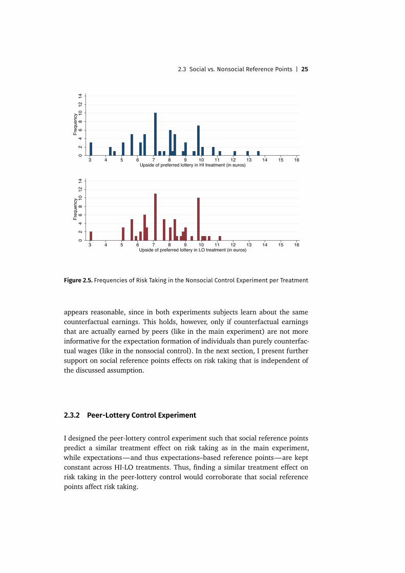
Figure 2.5 shows that active subjects in the nonsocial control experiment chosefairly similar lotteries across treatments. This is also reflected in the fact that theaverage chosen upsides were almost identical in HI and LO. In the LO treatment,active subjects chose an average upside of €7.62. In the HI treatment, the aver-age preferred upside of was €7.65. Additionally, across both treatments, samefrequency of lottery choices with upsides larger than €8 was roughly the same.
In the following, I present the main results of the paper: the treatment ef-fects on risk taking in the main experiment are significantly larger than in thenonsocial control. This allows to identify social reference points on risk taking.I replicate Results 1, 3, and 4 in a difference (between main experiment andnonsocial control) in differences (between HI-LO treatments) analysis.
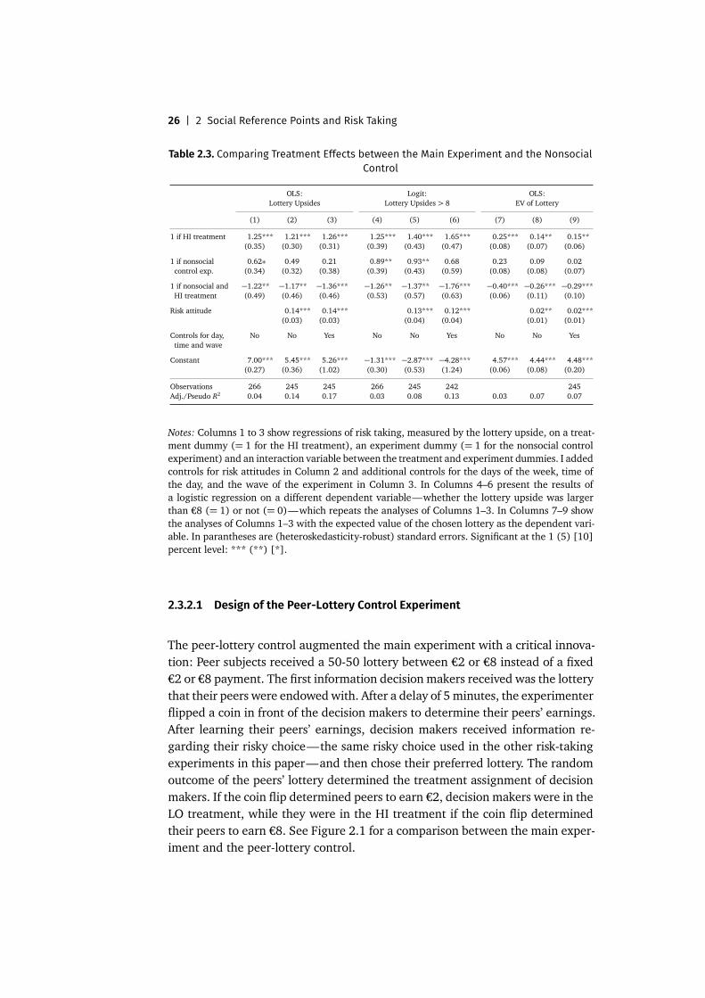
I regress the upside choices of the decision makers and active subjects, re-spectively, on a treatment dummy (= 1 if HI), on an experiment dummy (= 1if nonsocial control), and an interaction term of the two. The coefficient of theinteraction term estimates the difference in differences treatment effect on risktaking. Table 2.3 reports the results of such difference-in-differences estimations.It turns out that the coefficients on the interaction term are significantly smallerthan zero. Thus, the differences on risk-taking behavior reported in Results 1, 3,and 4 are significantly smaller in the nonsocial control compared to the mainexperiment.
Result 5. The difference in risk taking reported in Result 1 is significantly largerin the main experiment than in the nonsocial control. The difference in expectedvalues reported in Result 3 is significantly larger in the main experiment than inthe nonsocial control. The difference of lottery choices with an upside larger than€8 reported in Result 4 is significantly larger in the main treatment than in thenonsocial control.
Result 5 provides evidence that the treatment effects on risk taking of themain experiment identify social reference point effects rather than nonsocial—e.g., expectations-based—reference points. This evidence rests on the assump-tion that potential differences in expectations–based reference points are con-stant between the main experiment and the nonsocial control. This assumption
2.3 Social vs. Nonsocial Reference Points | 250
24
68
1012
14Fr
eque
ncy
3 4 5 6 7 8 9 10 11 12 13 14 15 16Upside of preferred lottery in HI treatment (in euros)
02
46
810
1214
Freq
uenc
y
3 4 5 6 7 8 9 10 11 12 13 14 15 16Upside of preferred lottery in LO treatment (in euros)
Figure 2.5. Frequencies of Risk Taking in the Nonsocial Control Experiment per Treatment
appears reasonable, since in both experiments subjects learn about the samecounterfactual earnings. This holds, however, only if counterfactual earningsthat are actually earned by peers (like in the main experiment) are not moreinformative for the expectation formation of individuals than purely counterfac-tual wages (like in the nonsocial control). In the next section, I present furthersupport on social reference points effects on risk taking that is independent ofthe discussed assumption.
2.3.2 Peer-Lottery Control Experiment
I designed the peer-lottery control experiment such that social reference pointspredict a similar treatment effect on risk taking as in the main experiment,while expectations—and thus expectations–based reference points—are keptconstant across HI-LO treatments. Thus, finding a similar treatment effect onrisk taking in the peer-lottery control would corroborate that social referencepoints affect risk taking.
26 | 2 Social Reference Points and Risk Taking
Table 2.3. Comparing Treatment Effects between the Main Experiment and the NonsocialControl
OLS: Logit: OLS:Lottery Upsides Lottery Upsides > 8 EV of Lottery
(1) (2) (3) (4) (5) (6) (7) (8) (9)
1 if HI treatment 1.25*** 1.21*** 1.26*** 1.25*** 1.40*** 1.65*** 0.25*** 0.14** 0.15**(0.35) (0.30) (0.31) (0.39) (0.43) (0.47) (0.08) (0.07) (0.06)
1 if nonsocial 0.62∗ 0.49 0.21 0.89** 0.93** 0.68 0.23 0.09 0.02control exp. (0.34) (0.32) (0.38) (0.39) (0.43) (0.59) (0.08) (0.08) (0.07)
1 if nonsocial and −1.22** −1.17** −1.36*** −1.26** −1.37** −1.76*** −0.40*** −0.26*** −0.29***HI treatment (0.49) (0.46) (0.46) (0.53) (0.57) (0.63) (0.06) (0.11) (0.10)
Risk attitude 0.14*** 0.14*** 0.13*** 0.12*** 0.02** 0.02***(0.03) (0.03) (0.04) (0.04) (0.01) (0.01)
Controls for day, No No Yes No No Yes No No Yestime and wave
Constant 7.00*** 5.45*** 5.26*** −1.31*** −2.87*** −4.28*** 4.57*** 4.44*** 4.48***(0.27) (0.36) (1.02) (0.30) (0.53) (1.24) (0.06) (0.08) (0.20)
Observations 266 245 245 266 245 242 245Adj./Pseudo R2 0.04 0.14 0.17 0.03 0.08 0.13 0.03 0.07 0.07
Notes: Columns 1 to 3 show regressions of risk taking, measured by the lottery upside, on a treat-ment dummy (= 1 for the HI treatment), an experiment dummy (= 1 for the nonsocial controlexperiment) and an interaction variable between the treatment and experiment dummies. I addedcontrols for risk attitudes in Column 2 and additional controls for the days of the week, time ofthe day, and the wave of the experiment in Column 3. In Columns 4–6 present the results ofa logistic regression on a different dependent variable—whether the lottery upside was largerthan €8 (= 1) or not (= 0)—which repeats the analyses of Columns 1–3. In Columns 7–9 showthe analyses of Columns 1–3 with the expected value of the chosen lottery as the dependent vari-able. In parantheses are (heteroskedasticity-robust) standard errors. Significant at the 1 (5) [10]percent level: *** (**) [*].
2.3.2.1 Design of the Peer-Lottery Control Experiment
The peer-lottery control augmented the main experiment with a critical innova-tion: Peer subjects received a 50-50 lottery between €2 or €8 instead of a fixed€2 or €8 payment. The first information decision makers received was the lotterythat their peers were endowedwith. After a delay of 5minutes, the experimenterflipped a coin in front of the decision makers to determine their peers’ earnings.After learning their peers’ earnings, decision makers received information re-garding their risky choice—the same risky choice used in the other risk-takingexperiments in this paper—and then chose their preferred lottery. The randomoutcome of the peers’ lottery determined the treatment assignment of decisionmakers. If the coin flip determined peers to earn €2, decision makers were in theLO treatment, while they were in the HI treatment if the coin flip determinedtheir peers to earn €8. See Figure 2.1 for a comparison between the main exper-iment and the peer-lottery control.
2.3 Social vs. Nonsocial Reference Points | 270
24
68
1012
14Fr
eque
ncy
3 4 5 6 7 8 9 10 11 12 13 14 15 16Upside of preferred lottery in HI treatment (in euros)
02
46
810
1214
Freq
uenc
y
3 4 5 6 7 8 9 10 11 12 13 14 15 16Upside of preferred lottery in LO treatment (in euros)
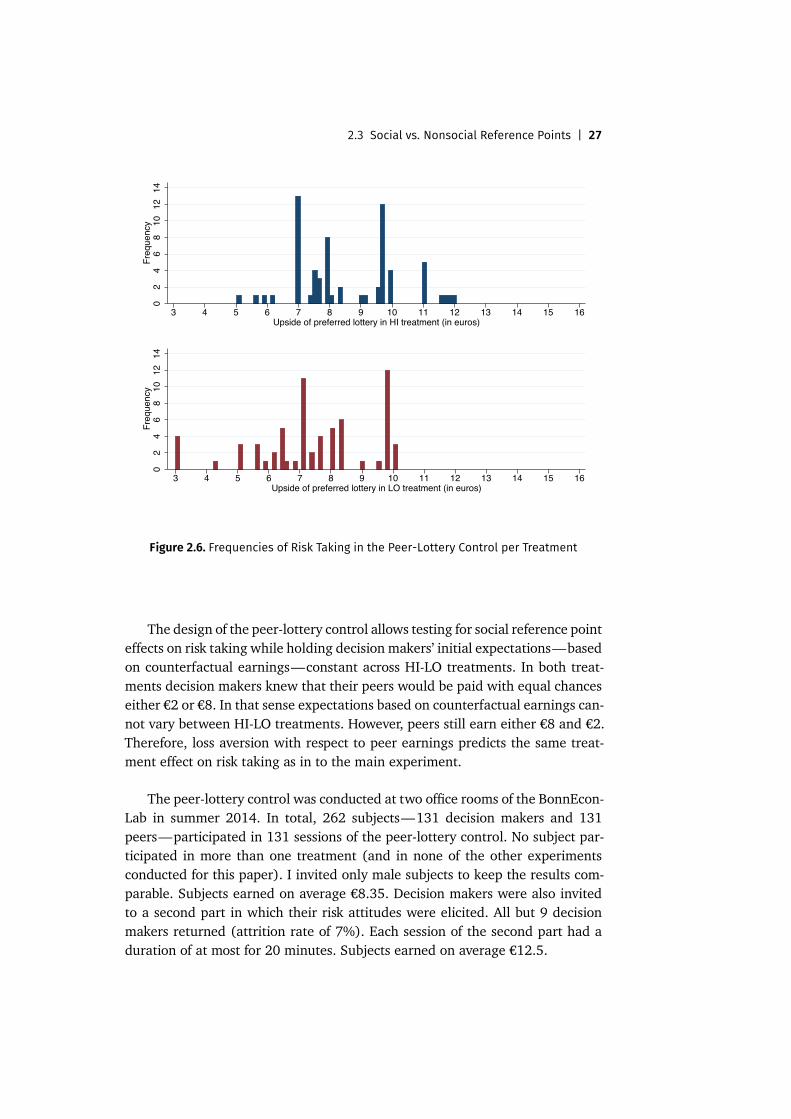
Figure 2.6. Frequencies of Risk Taking in the Peer-Lottery Control per Treatment
The design of the peer-lottery control allows testing for social reference pointeffects on risk taking while holding decision makers’ initial expectations—basedon counterfactual earnings—constant across HI-LO treatments. In both treat-ments decision makers knew that their peers would be paid with equal chanceseither €2 or €8. In that sense expectations based on counterfactual earnings can-not vary between HI-LO treatments. However, peers still earn either €8 and €2.Therefore, loss aversion with respect to peer earnings predicts the same treat-ment effect on risk taking as in to the main experiment.
The peer-lottery control was conducted at two office rooms of the BonnEcon-Lab in summer 2014. In total, 262 subjects—131 decision makers and 131peers—participated in 131 sessions of the peer-lottery control. No subject par-ticipated in more than one treatment (and in none of the other experimentsconducted for this paper). I invited only male subjects to keep the results com-parable. Subjects earned on average €8.35. Decision makers were also invitedto a second part in which their risk attitudes were elicited. All but 9 decisionmakers returned (attrition rate of 7%). Each session of the second part had aduration of at most for 20 minutes. Subjects earned on average €12.5.

28 | 2 Social Reference Points and Risk Taking
Table 2.4. Comparing Treatment Effects between the Peer-Lottery Control and theNonsocial Control
OLS: Logit: OLS:Lottery Upsides Lottery Upsides > 8 EV of Lottery
(1) (2) (3) (4) (5) (6) (7) (8) (9)
1 if HI treatment 1.20*** 0.97*** 1.04*** 0.59∗ 0.44 0.71∗ 0.09 0.08 0.09(0.30) (0.32) (0.34) (0.36) (0.39) (0.41) (0.07) (0.07) (0.07)
1 if nonsocial 0.18 0.04 0.39 0.21 0.14 0.23 0.06 0.2 0.13control exp. (0.31) (0.31) (0.43) (0.36) (0.37) (0.55) (0.08) (0.07) (0.08)
1 if nonsocial and −1.17** −0.95** −1.01*∗ −0.61 −0.43 −0.75 −0.24** −0.21∗ −0.21∗HI treatment (0.46) (0.47) (0.48) (0.50) (0.54) (0.56) (0.11) (0.11) (0.11)
Risk attitude 0.11*** 0.11*** 0.10*** 0.11*** 0.16**(0.03) (0.03) (0.03) (0.04) (0.01)
Controls for day, No No Yes No No Yes No No Yestime and wave
Constant 7.44*** 6.31*** 5.48*** −0.63** −1.69*** −4.03*** 4.74*** 4.57*** 4.42***(0.23) (0.42) (0.94) (0.26) (0.46) (1.46) (0.06) (0.12) (0.22)
Observations 265 241 241 265 241 240 265 241 241Adj./Pseudo R2 0.05 0.10 0.08 0.01 0.03 0.10 0.01 0.04 0.03
Notes: In Columns 1 to 3 show regressions of risk taking, measured by the chosen lottery upside,on a treatment dummy (= 1 for the HI treatment), an experiment dummy (= 1 for the nonsocialcontrol experiment) and an interaction between the later two. I added controls for risk attitudes tothis regression In Column 2 and additional controls for the days of the week, time of the day, andthe wave of the experiment in Column 3. Columns 4–6 present the results of a logistic regressionof a different dependent variable—whether the chosen lottery upside was larger than €8 (= 1)or not (= 0)—which repeats the analyses of Columns 1–3. Columns 7–9 show the analyses ofColumns 1–3 with the expected value of the chosen lottery as the dependent variable. I state(heteroskedasticity-robust) standard errors in parentheses. Significant at the 1 (5) [10] percentlevel: *** (**) [*].
2.3.2.2 Peer-Lottery Control Results
The results of the peer-lottery control provide further support for social refer-ence point effects on risk taking. On average, decision makers chose an averageupside of €8.64 in HI and of €7.44 in LO. This difference in risk taking is signifi-cant in an OLS regression and significantly larger than in the nonsocial control,see Columns 1 to 3 of Table 2.4. Additionally, the average difference in expectedvalues between HI-LO treatments is larger in the peer-lottery control relativeto the main experiment, see Columns 7 to 9. While the likelihood that decisionmakers chose upsides larger than €8 is larger in the HI treatment than in theLO treatment, see Row 1 and Columns 4 to 6, this difference is not significantlylarger than in the nonsocial control, see Row 3 and Columns 4 to 6.
Result 6. Result 5 can be replicated in difference-in-difference analyses on risktaking between HI-LO treatments in the peer-lottery and nonsocial control exper-iments. The treatment effect on upsides, expected values, and frequency of upside
2.4 Conclusion | 29
choices above €8 is larger in the peer-lottery control than in the nonsocial control.The former two are significant, while the latter is not.
In sum, these findings indicate that the treatment effect on risk taking ob-served in the main experiment is caused by social reference points rather thannonsocial reference points. When keeping expectations constant across treat-ments and only varying social reference points, decision makers behaved simi-larly relative to the main experiment.
2.4 Conclusion
Using a simple laboratory experiment, I provide causal evidence for social ref-erence point effects on risk taking. Decision makers increase their risk takingin light of relatively larger peer earnings—in the absence of any other socialmotives and forms of peer effects. The observed risk taking is consistent with anaversion against earning less than others. These findings provide clean evidencethat relative concerns affect human behavior.
The interpretation of the main experiment is substantiated by means of twocontrol experiments. Most importantly, when removing motives based on socialreference point but maintaining the potential for alternative explanations basedon nonsocial—e.g., expectations-based—reference points constant, risk takingis not affected. Difference-in-difference analyses between the main and nonso-cial control experiments support the interpretation that the treatment effect onrisk taking in the main experiment identifies social reference points effects.
The results of this study are applicable to the recent literature on the use ofrelative concerns at the workplace (Moldovanu et al., 2007) Performance rank-ings may incentivize workers to increase their effort in order to improve relativeperformance—independent of additional pecuniary incentives. This study sug-gests, that apart from effort, the willingness to take risk of workers may also beaffected by such social comparisons. Any principal that may want to make use ofsocial incentives should, therefore, take the potential effect on risk taking intoaccount as well. My results also suggest that even in the case that wages arenot made transparent through performance rankings, but individuals receiveprivate signals of their relative outcomes, behavioral consequences should beanticipated by principles.
The findings of this study imply that salient peer outcomes affect the refer-ence point of individuals. In my study, subjects were presented with one peer out-come only, but in many applications, individuals observe multiple peer outcomes(Falk and Knell, 2004). An interesting avenue for future research, therefore, isto attain a better understanding, both theoretically and empirically, of whichpeer outcomes individuals will find most salient or choose from as a comparisonwhen confronted with multiple sources for social reference points.
30 | 2 Social Reference Points and Risk Taking
References
Abeler, Johannes, Armin Falk, Lorenz Goette, and David Huffman (2011): “Reference Pointsand Effort Provision.” American Economic Review, 101 (2), 470–492. [6]
Adams, J. Stacy (1963): “Toward an Understanding of Inequity.” Journal of Abnormal andSocial Psychology, 67 (5), 422–436. [6]
Allen, Eric J., Patricia M. Dechow, Devin G. Pope, and George Wu (2014): “Reference-Dependent Preferences: Evidence from Marathon Runners.” Working Paper. [6]
Andreoni, James and William T. Harbaugh (2010): “Unexpected Utility: Experimental Testsof Five Key Questions about Preferences over Risk.” Working Paper. [13]
Ariely, Dan, Uri Gneezy, George Loewenstein, and Nina Mazar (2009): “Large Stakes andBig Mistakes.” Review of Economic Studies, 76 (2), 451–469. [6]
Ball, Sheryl, Catherine Eckel, Philip J. Grossman, and William Zame (2001): “Status in Mar-kets.” Quarterly Journal of Economics, 116 (1), 161–188. [11]
Bartling, Björn, Leif Brandes, andDaniel Schunk (2015): “Expectations as Reference Points:Field Evidence from Professional Soccer.” Management Science, 61 (11), 2646–2661.[6]
Bénabou, Roland and Jean Tirole (2006): “Incentives and Prosocial Behavior.” AmericanEconomic Review, 96 (5), 1652–1678. [6]
Benartzi, Shlomo and Richard H. Thaler (1995): “Myopic Loss Aversion and the Equity Pre-mium Puzzle.” Quarterly Journal of Economics, 110 (1), 73–92. [6]
Bolton, Gary E. and Axel Ockenfels (2000): “ERC: A Theory of Equity, Reciprocity, and Com-petition.” American Economic Review, 90 (1), 166–193. [6, 16]
Bursztyn, Leonardo, Florian Ederer, Bruno Ferman, and Noam Yuchtman (2014): “Under-standing Mechanisms Underlying Peer Effects: Evidence From a Field Experiment onFinancial Decisions.” Econometrica, 82 (4), 1273–1301. [11]
Camerer, Colin F., Linda Babcock, George Loewenstein, and Richard H. Thaler (1997): “La-bor Supply of New York City Cabdrivers: One Day at a Time.” Quarterly Journal of Eco-nomics, 112 (2), 407–441. [6]
Card, David, Alexandre Mas, Enrico Moretti, and Emmanuel Saez (2012): “Inequality atWork: The Effect of Peer Salaries on Job Satisfaction.” American Economic Review,102 (6), 2981–3003. [6, 11]
Charness, Gary andMatthewRabin (2002): “Understanding Social Preferences with SimpleTests.” Quarterly Journal of Economics, 117 (3), 817–869. [6, 16]
Clark, Andrew E., Paul Frijters, and Michael A. Shields (2008): “Relative Income, Happiness,Utility: An Explanation for the Easterlin Paradox and Other Puzzles.” Journal of Eco-nomic Literature, 46 (1), 95–144. [16]
Crawford, Vincent P. and Juanjuan Meng (2011): “New York City Cab Drivers’ Labor SupplyRevisited: Reference-Dependent Preferences with Rational-Expectations Targets forHours and Income.” American Economic Review, 101 (5), 1912–1932. [6]
DellaVigna, Stefano, Attila Lindner, Balazs Reizer, and Johannes F. Schmieder (2015):“Reference-Dependent Job Search: Evidence from Hungary.” Report. [6]
Dohmen, Thomas, Armin Falk, David Huffman, Uwe Sunde, Jürgen Schupp, andGert G.Wag-ner (2011): “Individual Risk Attitudes: Measurement, Determinants, and BehavioralConsequences.” Journal of the European Economic Association, 9 (3), 522–550. [7]
References | 31
Duflo, Esther and Emmanuel Saez (2002): “Participation and Investment Decisions in aTetirement Plan: The Influence of Colleagues’ Choices.” Journal of Public Economics,85 (1), 121–148. [11]
Engelmann, Dirk and Martin Strobel (2004): “Inequality Aversion, Efficiency, and MaximinPreferences in Simple Distribution Experiments.” American Economic Review, 94 (4),857–869. [6]
Ericson, Keith M. and Andreas Fuster (2011): “Expectations as Endowments: Evidence onReference-Dependent Preferences from Exchange and Valuation Experiments.” Quar-terly Journal of Economics, 126 (4), 1879–1907. [6]
Falk, Armin and Urs Fischbacher (2006): “A Theory of Reciprocity.” Games and EconomicBehavior, 54 (2), 293–315. [6, 16]
Falk, Armin and Andrea Ichino (2006): “Clean Evidence on Peer Effects.” Journal of LaborEconomics, 24 (1), 39–57. [11]
Falk, Armin and Markus Knell (2004): “Choosing the Joneses: Endogenous Goals and Ref-erence Standards.” Scandinavian Journal of Economics, 106 (3), 417–435. [29]
Fehr, Ernst and Lorenz Goette (2007): “Work More if Wages Are High? Evidence from a DoWorkers Randomized Field Experiment.” American Economic Review, 97 (1), 298–317.[6]
Fehr, Ernst and Klaus M. Schmidt (1999): “A Theory Of Fairness, Competition, and Cooper-ation.” Quarterly Journal of Economics, 114 (3), 817–868. [6, 16]
Festinger, Leon (1954): “A Theory of Social Comparison Processes.” Human Relations, 1,117–140. [6]
Fischbacher, Urs (2007): “z-Tree: Zurich Toolbox for Ready-Made Economic Experiments.”Experimental Economics, 10 (2), 171–178. [14]
Fliessbach, Klaus, Bernd Weber, Peter Trautner, Thomas Dohmen, Uwe Sunde, Christian E.Elger, and Armin Falk (2007): “Social comparison affects reward-related brain activityin the human ventral striatum.” Science, 318 (5854), 1305–1308. [6]
Frank, Robert H. (1985): “The Demand for Unobservable and Other Nonpositional Goods.”American Economic Review, 75 (1), 101–116. [6]
Genesove, David and Christopher Mayer (2001): “Loss Aversion and Seller Behavior: Evi-dence from the Housing Market.” Quarterly Journal of Economics, 116 (4), 1233–1260.[6]
Gill, David and Victoria Prowse (2012): “A Structural Analysis of Disappointment Aversionin a Real Effort Competition.” American Economic Review, 102 (1), 469–503. [6]
Gneezy, Uri, LorenzGoette, Charles Sprenger, and Florian Zimmermann (2013): “The Limitsof Expectations-Based Reference Dependence.” Working Paper. [6]
Gneezy, Uri and Jan Potters (1997): “An Experiment on Risk Taking and Evaluation Periods.”Quarterly Journal of Economics, 112 (2), 631–645. [6]
Greiner, Ben (2004): “An Online Recruitment System For Economic Experiments.”Forschung und Wissenschaftliches Rechnen, 63, 79–93. [14]
Heffetz, Ori (2011): “A Test of Conspicuous Consumption: Visibility and Income Elasticities.”Review of Economics and Statistics, 93 (4), 1101–1117. [11]
Heffetz, Ori and Robert Frank (2011): “Preferences for Status: Evidence and Economic Im-plications.” In Handbook of Social Economics. Ed. by Jess Benhabib, Alberto Bisin, andMatthew Jackson. Elsevier B.V., 69–92. [11]
Heffetz, Ori and John A. List (2014): “Is the Endowment Effect an Expectations Effect?”Journal of the European Economic Association, 12 (5), 1396–1422. [6]
32 | 2 Social Reference Points and Risk Taking
Heidhues, Paul and Botond Kőszegi (2008): “Competition and Price Variation when Con-sumers Are Loss Averse.” American Economic Review, 98 (4), 1245–1268. [6]
Herweg, Fabian, Daniel Müller, and Philipp Weinschenk (2010): “Binary Payment Schemes:Moral Hazard and Loss Aversion.” American Economic Review, 100 (5), 2451–2477. [6]
Huberman, Bernardo A., Christoph H. Loch, and Ayse Onculer (2004): “Status As a ValuedResource.” Social Psychology Quarterly, 67 (1), 103–114. [11]
Kahneman, Daniel, Jack L. Knetsch, and Richard H. Thaler (1990): “Experimental Tests ofthe Endowment Effect and the Coase Theorem.” Journal of Political Economy, 98 (6),1325–1348. [6]
Kahneman, Daniel and Amos Tversky (1979): “Prospect Theory: An Analysis of Decisionunder Risk.” Econometrica, 47 (2), 263–292. [5, 6]
Kőszegi, Botond and Matthew Rabin (2006): “A Model of Reference-Dependent Prefer-ences.” Quarterly Journal of Economics, 121 (4), 1133–1165. [6, 8, 16]
Kőszegi, Botond and Matthew Rabin (2007): “Reference-Dependent Risk Attitudes.” Amer-ican Economic Review, 97 (4), 1047–1073. [6, 8, 16]
Kőszegi, Botond and Matthew Rabin (2009): “Reference-Dependent Consumption Plans.”American Economic Review, 99 (3), 909–936. [6]
Kuhn, Peter, Peter Kooreman, Adriaan R. Soetevent, and Arie Kapteyn (2011): “The Effectsof Lottery Prizes on Winners and their Neighbors: Evidence from the Dutch PostcodeLottery.” American Economic Review, 101 (5), 2226–2247. [11]
Levine, David K. (1998): “Modeling Altruism and Spitefulness in Experiments.” Review ofEconomic Dynamics, 1 (3), 593–622. [6]
Linde, Jona and Joep Sonnemans (2012): “Social Comparison and Risky Choices.” Journalof Risk and Uncertainty, 44 (1), 45–72. [6]
Mas, Alexandre (2006): “Pay, Reference Points, and Police Performance.” Quarterly Journalof Economics, 121 (3), 783–821. [6]
Mas, Alexandre and Enrico Moretti (2009): “Peers at Work.” American Economic Review,99 (1), 112–145. [11]
Moldovanu, Benny, Aner Sela, and Xianwen Shi (2007): “Contests for Status.” Journal ofPolitical Economy, 115 (2), 338–363. [29]
Odean, Terrance (1998): “Are Investors Reluctant to Realize Their Losses?” Journal of Fi-nance, 53 (5), 1775–1798. [6]
Pope, Devin G. and Maurice E. Schweitzer (2011): “Is Tiger Woods Loss Averse? PersistentBias in the Face of Experience, Competition, and High Stakes.” American EconomicReview, 101 (1), 129–157. [6]
Rabin, Matthew (2000): “Risk Aversion and Expected-Utility Theory: A Calibration Theo-rem.” Econometrica, 68 (5), 1281–1292. [6]
Rees-Jones, Alex (2014): “Loss Aversion Motivates Tax Sheltering: Evidence from U.S. TaxReturns.” Working Paper. [6]
Sacerdote, Bruce (2001): “Peer Effects with Random Assignment: Results for DartmouthRoommates.” Quarterly Journal of Economics, 116 (2), 681–704. [11]
Shefrin, Hersh and Meir Statman (1985): “The Disposition to Sell Winners Too Early andRide Losers Too Long: Theory and Evidence.” Journal of Finance, 40 (3), 777–790. [6]
Song, Changcheng (2012): “An Experiment on Reference Points and Expectations.” WorkingPaper. [10]
Sprenger, Charles (2015): “An Endowment Effect for Risk: Experimental Tests of StochasticReference Points.” Journal of Political Economy, 123 (6), 1456–1499. [6]
2.A Instructions | 33
Taylor, Chris (2011): “Tight budgets, Wild Markets Hurt Investment Clubs.” avail-able at http://www.reuters.com/article/2011/12/12/us-usa-investing-clubs-idUSTRE7BB19M20111212. [11]
Veblen, Thorstein (1899): The theory of the leisure class. New York: Macmillan. [6]
Appendix 2.A Instructions
Main experiment, decision maker, HI [LO] treatment
In this experiment, your task is to complete a survey. Participant B completesthe same survey.
The both of you receive the show-up fee for your participation in this exper-iment. Participant B receives an additional payment of €8 [€2]. You can alsoreceive an additional payment. Your additional payment is not determined yet.Your additional payment depends on your decision-making before you start com-pleting the survey.
Notice, participant B does not learn your additional payment and leaves thelab before you do.
[next screen]
Your additional payment depends on your choice between different options.
One option is the certain payment of €3.
All other options are binary lotteries. Among all options, one outcome is 0.You can choose the other outcome freely between a minimum and maximumoutcome. The higher you choose this outcome, the lower is the likelihood thatyou receive it.
We use urns to display lotteries graphically in this experiment. If you choosea lottery, then the computer randomly chooses which outcome you receive asyour additional payment. This happens at the end of the experiment, after youcompleted the survey and are paid in cash.
Nonsocial control, active subject, HI [LO] treatment
In this experiment, your task is to complete a survey. If you would have beenparticipant B, you would have to complete the same survey.
34 | 2 Social Reference Points and Risk Taking
In both roles you receive the show-up fee for your participation in this exper-iment. If you would have been participant B, you would receive an additionalpayment of €8 [€2]. As participant A, you can also receive an additional pay-ment. Your additional payment is not determined yet. Your additional paymentdepends on your decision-making before you start completing the survey.
[next screen]
Your additional payment depends on your choice between different options.
One option is the certain payment of €3.
All other options are binary lotteries. Among all options, one outcome is 0.You can choose the other outcome freely between a minimum and maximumoutcome. The higher you choose this outcome, the lower is the likelihood thatyou receive it.
We use urns to display lotteries graphically in this experiment. If you choosea lottery, then the computer randomly chooses which outcome you receive asyour additional payment. This happens at the end of the experiment, after youcompleted the survey and are paid in cash.
Peer-lottery control, decision maker, HI [LO] treatment
In this experiment, your task is to complete a survey. Participant B completesthe same survey.
The both of you receive the show-up fee for your participation in this ex-periment. Participant B receives an additional payment of either €8 or €2. It israndom whether participant B receives €8 or €2. A coin toss will be perfomed infront of you to determine the additional payment of participant B. With heads,participant B earns €2 and with tails €8. Please wait until the experimenter willcome to you to perform the coin toss.
[next screen]
The coin toss determined that participant B receives €8 [€2] additionally.You can also receive an additional payment. Your additional payment is not de-termined yet. Your additional payment depends on your decision-making beforeyou start completing the survey.
Notice, participant B does not learn your additional payment and leaves thelab before you do.
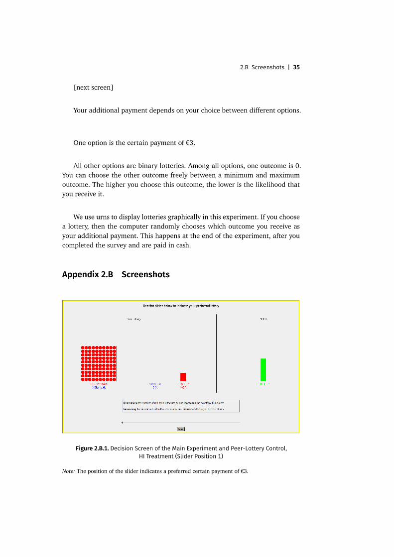
2.B Screenshots | 35
[next screen]
Your additional payment depends on your choice between different options.
One option is the certain payment of €3.
All other options are binary lotteries. Among all options, one outcome is 0.You can choose the other outcome freely between a minimum and maximumoutcome. The higher you choose this outcome, the lower is the likelihood thatyou receive it.
We use urns to display lotteries graphically in this experiment. If you choosea lottery, then the computer randomly chooses which outcome you receive asyour additional payment. This happens at the end of the experiment, after youcompleted the survey and are paid in cash.
Appendix 2.B Screenshots
Figure 2.B.1. Decision Screen of the Main Experiment and Peer-Lottery Control,HI Treatment (Slider Position 1)
Note: The position of the slider indicates a preferred certain payment of €3.
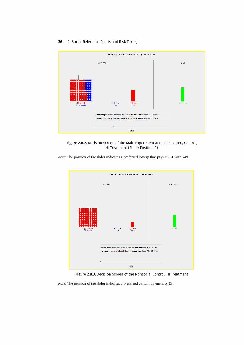
36 | 2 Social Reference Points and Risk Taking
Figure 2.B.2. Decision Screen of the Main Experiment and Peer-Lottery Control,HI Treatment (Slider Position 2)
Note: The position of the slider indicates a preferred lottery that pays €6.51 with 74%.
Figure 2.B.3. Decision Screen of the Nonsocial Control, HI Treatment
Note: The position of the slider indicates a preferred certain payment of €3.

3
Concentration Bias inIntertemporal Choice?
Joint with Holger Gerhardt and Louis Strang
3.1 Introduction
Any decision that wemake has intertemporal consequences. These consequencesoften stretch over numerous days, months, or even years. For instance, missingout on exercising at the gym today deteriorates physical well-being each follow-ing day; or aspiring to a bonus payment at the end of the year may animateovertime work each day until the end of the year. According to exponentialand hyperbolic discounting—the canonical approaches to intertemporal deci-sion making in economics—individuals evaluate a decision by aggregating allits consequences into a weighted sum, with the weights reflecting their timepreferences. Individuals then choose the option that yields the highest sum.Whether constant and hyperbolic (present-biased) discounting are sufficientto capture all important aspects of intertemporal decision making, however, re-mains an open question.
In this paper, we contribute to the understanding of intertemporal deci-sion making by studying an attention-based approach to how individuals (mis-)aggregate intertemporal consequences. The potential of this approach stemsfrom a pervasive characteristic of intertemporal decisions: positive consequencesare often concentrated in a single, attention-grabbing period, while negativeconsequences are dispersed in non-tangible doses over numerous periods. Forinstance, avoiding the hassle of exercising at the gym today marginally deterio-rates physical well-being each following day; or the prospect of receiving a large
? We thank Thomas Dohmen, Armin Falk, Lorenz Götte, Johannes Haushofer, David Laibson,and Matthew Rabin for helpful comments.
38 | 3 Concentration Bias in Intertemporal Choice
bonus payment at the end of the year may come at the cost of working halfan hour overtime each day until then. In light of the evidence from cognitivepsychology that human perception is an important driver of individual decisionmaking (see, e.g., Kahneman, 2003), this asymmetry may give rise to attention-based effects regarding how individuals aggregate intertemporal consequencesand, thus, how they make intertemporal decisions.
The attention-based approach that we build on generates an overweightingof concentrated consequences relative to dispersed consequences. Thus, weight-ing of intertemporal consequences no longer solely reflects time preferences à laconstant or present-biased discounting, but entails an asymmetric overweight-ing of particular consequences. Kőszegi and Szeidl (2013) recently introduceda model of economic decision making that formalizes such overweighting. Theirmodel is based on the assumption that individuals weight the consequences ina period the more, the greater the difference between the maximum and min-imum consequences in that period. Take, for instance, the example of gettinga bonus payment at the end of the year at the expense of some overtime workeach day until then or not getting any bonus payment at the benefit of no over-time work. The day the bonus payment is received is characterized by a largedifference between consequences: the bonus payment is paid out or not. Thedays prior to the bonus payment are characterized by smaller differences be-tween the consequences: little overtime work or none. Similarly, materializingor avoiding the hassle of going to the gym entails a greater distance in conse-quences today than for any later period, because in these later periods, eachgym attendance generates only marginal changes in physical well-being. In gen-eral, consequences that are more concentrated—i.e., that are spread over fewerperiods—than equal-sized dispersed consequences imply a greater per-perioddifference and are thus overweighted, according to the model.
Such concentration bias—when added to constant and present-biaseddiscounting—yields two testable predictions on intertemporal decision mak-ing. First, individuals may behave overly impatient—relative to constant andpresent-biased discounting as the benchmark—when concentrated positive con-sequences of behaving impatiently precede its dispersed negative consequences.For instance, suffering from a little back pain each day in the future may bedisregarded when this allows avoiding the attention-grabbing hassle of going tothe gym now. Second, when concentrated positive consequences of behaving pa-tiently succeed dispersed negative consequences, individuals may behave overlypatient—relative to both exponential and hyperbolic discounting. For instance,little overtime work each day may be neglected in exchange for receiving anattention-grabbing bonus payment in the future. While concentration bias seemsintuitively compelling, there exists—to our knowledge—no empirical investiga-tion of it yet.
3.1 Introduction | 39
We designed a novel laboratory experiment to fill this gap. In particular, thedesign of our experiment allows us to investigate whether individuals systemati-cally overweight concentrated intertemporal consequences relative to dispersedconsequences. In doing so, we test both directions of concentration bias: Dosubjects behave more impatiently when the negative consequences of impatientbehavior are dispersed over multiple later periods? Do they behave more pa-tiently when the negative consequences of patient behavior are dispersed overmultiple earlier periods?
In our experiment, subjects were endowed with multiple earnings sequences.Each earnings sequence specified a series of 9 money transfers to subjects’ bankaccounts at given dates in the future. Subjects decided whether to decrease ear-lier payments at the benefit of increasing later payments. The sum total wasthe greater, the more money subjects allocated to later periods. The larger theamount of money that subjects decided to receive at later payment dates—i.e.,the more they were willing to wait in order to receive an overall larger sumof money—the more patient we consider them (see Andreoni and Sprenger(2012)).
To test whether concentration bias affects intertemporal choices, we variedwithin-subject whether the intertemporal allocation was exclusively betweenconcentrated consequences (CONC) or whether there were both concentratedand dispersed consequences (DISP). Put differently, between conditions, wechanged the shape of the intertemporal budget constraint (the “intertemporal al-location technology”). We test whether subjects’ decisions differed significantlybetween conditions.
In order to investigate both directions of a potential concentration bias, wecompare intertemporal decisions between earnings sequences in CONCa andDISPa as well as between earnings sequences in CONCb and DISPb, as describedin the following. In condition CONCa, subjects received a sequence of 9 datedmoney transfers that were separated by several weeks each. We can express thissequence as the vector
[1 + B (1 − x), 1, 1, 1, 1, 1, 1, 1, 1 + RBx],
with the ith entry specifying the euro amount of the ith payment. R≡ 1+ r isan interest factor (with r being the nominal interest rate), and B is the endow-ment in the first period. That is, R and B denote parameters of a given incomesequence (e.g., B = €11, r = 15%), while x is the subject’s choice variable. Bychoosing x ∈ {0, 1/100, 2/100, . . . , 1}, subjects decided what fraction of their firstpayment they would forego in exchange for receiving the remaining fractionplus interest at the last payment date. (For instance, with B = €11 and r = 15%,subjects could receive €1+ €12.60 as the last payment).
40 | 3 Concentration Bias in Intertemporal Choice
In condition DISPa, subjects received similar earnings sequences as inCONCa. The only difference between DISPa and CONCa was that RBx was notpaid at the last payment date, but was dispersed across the last payment dateand multiple earlier payment dates. In DISPa8, for instance, c was dispersedover the last payment date and 7 earlier payment dates. That is, the earningssequence given to subjects in DISPa8 can be represented as
�
1 + B (1 − x), 1 +RBx
8,1 +
RBx8
,1 +RBx
8, 1 +
RBx8
,
1 +RBx
8,1 +
RBx8
,1 +RBx
8, 1 +
RBx8
�
.
This means that in DISPa, the negative consequences of impatient behavior—i.e., of choosing a low x—were dispersed. In DISPa8, they took on the form ofsmall payments over the last 8 periods. In DISPa4 and DISPa2, we dispersedpayments over the last 4 and 2 periods, respectively. By contrast, in CONCa, thenegative consequence of allocating the entire amount to the soonest paymentdate was concentrated, and thus attention-grabbing, at the last payment date.
Concentration bias, therefore, predicts that individuals allocate less moneyto later payments in DISPa than in CONCa. Importantly, the present value ofDISPa is higher than that of CONCa. Thus, in contrast to concentration bias,both exponential and hyperbolic discounting predict that the amount allocatedto later periods in DISPa is at least as large as in CONCa.
In condition CONCb, subjects received similar sequences as in CONCa. Thatis, also CONCb involved intertemporal allocation of money between two concen-trated payments. CONCb differs from CONCa in that subjects received B (1− x)on the second-to-last payment date (instead of the first date):
[1, 1,1, 1,1,1, 1,1 + B (1 − x), 1 + RBx].
In the associated dispersed condition, DISPb, subjects were endowed withsimilar earnings sequences as in CONCb. The only difference between DISPBand CONCB was that B (1− x) was not paid at the second-to-last date, but wasdispersed over the second-to-last date and multiple earlier payment dates. InDISPb8, for instance, B (1− x) was dispersed over the second-to-last date and7 earlier dates. That is, the earnings sequence was of the type
�
1 +B (1 − x)
8, 1 +
B (1 − x)8
, 1 +B (1 − x)
8,1 +
B (1 − x)8
,
1 +B (1 − x)
8, 1 +
B (1 − x)8
, 1 +B (1 − x)
8,1 +
B (1 − x)8
,1 + RBx�
.
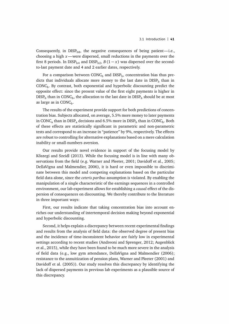
3.1 Introduction | 41
Consequently, in DISPb8, the negative consequences of being patient—i.e.,choosing a high x—were dispersed, small reductions in the payments over thefirst 8 periods. In DISPb4 and DISPb2, B (1− x) was dispersed over the second-to-last payment date and 4 and 2 earlier dates, respectively.
For a comparison between CONCb and DISPb, concentration bias thus pre-dicts that individuals allocate more money to the last date in DISPb than inCONCb. By contrast, both exponential and hyperbolic discounting predict theopposite effect: since the present value of the first eight payments is higher inDISPb than in CONCb, the allocation to the last date in DISPb should be at mostas large as in CONCb.
The results of the experiment provide support for both predictions of concen-tration bias. Subjects allocated, on average, 5.5%more money to later paymentsin CONCa than in DISPa decisions and 6.5% more in DISPb than in CONCb. Bothof these effects are statistically significant in parametric and non-parametrictests and correspond to an increase in “patience” by 9%, respectively. The effectsare robust to controlling for alternative explanations based on amere calculationinability or small-numbers aversion.
Our results provide novel evidence in support of the focusing model byKőszegi and Szeidl (2013). While the focusing model is in line with many ob-servations from the field (e.g. Warner and Pleeter, 2001; Davidoff et al., 2005;DellaVigna and Malmendier, 2006), it is hard or even impossible to discrimi-nate between this model and competing explanations based on the particularfield data alone, since the ceteris paribus assumption is violated. By enabling themanipulation of a single characteristic of the earnings sequences in a controlledenvironment, our lab experiment allows for establishing a causal effect of the dis-persion of consequences on discounting. We thereby contribute to the literaturein three important ways:
First, our results indicate that taking concentration bias into account en-riches our understanding of intertemporal decision making beyond exponentialand hyperbolic discounting.
Second, it helps explain a discrepancy between recent experimental findingsand results from the analysis of field data: the observed degree of present biasand the incidence of time-inconsistent behavior are fairly low in experimentalsettings according to recent studies (Andreoni and Sprenger, 2012; Augenblicket al., 2015), while they have been found to be much more severe in the analysisof field data (e.g., low gym attendance, DellaVigna and Malmendier (2006);resistance to the annuitization of pension plans, Warner and Pleeter (2001) andDavidoff et al. (2005)). Our study resolves this discrepancy by identifying thelack of dispersed payments in previous lab experiments as a plausible source ofthis discrepancy.
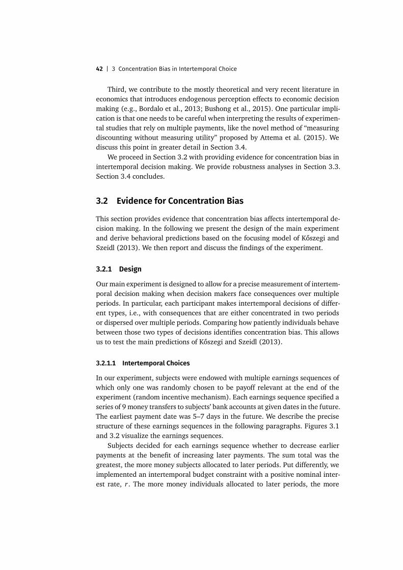
42 | 3 Concentration Bias in Intertemporal Choice
Third, we contribute to the mostly theoretical and very recent literature ineconomics that introduces endogenous perception effects to economic decisionmaking (e.g., Bordalo et al., 2013; Bushong et al., 2015). One particular impli-cation is that one needs to be careful when interpreting the results of experimen-tal studies that rely on multiple payments, like the novel method of “measuringdiscounting without measuring utility” proposed by Attema et al. (2015). Wediscuss this point in greater detail in Section 3.4.
We proceed in Section 3.2 with providing evidence for concentration bias inintertemporal decision making. We provide robustness analyses in Section 3.3.Section 3.4 concludes.
3.2 Evidence for Concentration Bias
This section provides evidence that concentration bias affects intertemporal de-cision making. In the following we present the design of the main experimentand derive behavioral predictions based on the focusing model of Kőszegi andSzeidl (2013). We then report and discuss the findings of the experiment.
3.2.1 Design
Ourmain experiment is designed to allow for a precisemeasurement of intertem-poral decision making when decision makers face consequences over multipleperiods. In particular, each participant makes intertemporal decisions of differ-ent types, i.e., with consequences that are either concentrated in two periodsor dispersed over multiple periods. Comparing how patiently individuals behavebetween those two types of decisions identifies concentration bias. This allowsus to test the main predictions of Kőszegi and Szeidl (2013).
3.2.1.1 Intertemporal Choices
In our experiment, subjects were endowed with multiple earnings sequences ofwhich only one was randomly chosen to be payoff relevant at the end of theexperiment (random incentive mechanism). Each earnings sequence specified aseries of 9 money transfers to subjects’ bank accounts at given dates in the future.The earliest payment date was 5–7 days in the future. We describe the precisestructure of these earnings sequences in the following paragraphs. Figures 3.1and 3.2 visualize the earnings sequences.
Subjects decided for each earnings sequence whether to decrease earlierpayments at the benefit of increasing later payments. The sum total was thegreatest, the more money subjects allocated to later periods. Put differently, weimplemented an intertemporal budget constraint with a positive nominal inter-est rate, r. The more money individuals allocated to later periods, the more
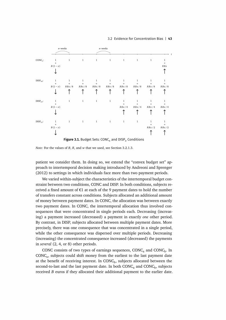
3.2 Evidence for Concentration Bias | 43
t
w weeks w weeks
CONCa: 1+
B (1− x)
↓
1 1 1 1 1 1 1 1+
R Bx
↑DISPa8: 1
+B (1− x)
↓
1+
R Bx /8
↑
1+
R Bx /8
↑
1+
R Bx /8
↑
1+
R Bx /8
↑
1+
R Bx /8
↑
1+
R Bx /8
↑
1+
R Bx /8
↑
1+
R Bx /8
↑DISPa4: 1
+B (1− x)
↓
1 1 1 1 1+
R Bx /4
↑
1+
R Bx /4
↑
1+
R Bx /4
↑
1+
R Bx /4
↑DISPa2: 1
+B (1− x)
↓
1 1 1 1 1 1 1+
R Bx /2
↑
1+
R Bx /2
↑Figure 3.1. Budget Sets: CONCa and DISPa Conditions
Note: For the values of B, R, and w that we used, see Section 3.2.1.3.
patient we consider them. In doing so, we extend the “convex budget set” ap-proach to intertemporal decision making introduced by Andreoni and Sprenger(2012) to settings in which individuals face more than two payment periods.
We varied within-subject the characteristics of the intertemporal budget con-straint between two conditions, CONC and DISP. In both conditions, subjects re-ceived a fixed amount of €1 at each of the 9 payment dates to hold the numberof transfers constant across conditions. Subjects allocated an additional amountof money between payment dates. In CONC, the allocation was between exactlytwo payment dates. In CONC, the intertemporal allocation thus involved con-sequences that were concentrated in single periods each. Decreasing (increas-ing) a payment increased (decreased) a payment in exactly one other period.By contrast, in DISP, subjects allocated between multiple payment dates. Moreprecisely, there was one consequence that was concentrated in a single period,while the other consequence was dispersed over multiple periods. Decreasing(increasing) the concentrated consequence increased (decreased) the paymentsin several (2, 4, or 8) other periods.
CONC consists of two types of earnings sequences, CONCa and CONCb. InCONCa, subjects could shift money from the earliest to the last payment dateat the benefit of receiving interest. In CONCb, subjects allocated between thesecond-to-last and the last payment date. In both CONCa and CONCb, subjectsreceived B euros if they allocated their additional payment to the earlier date.
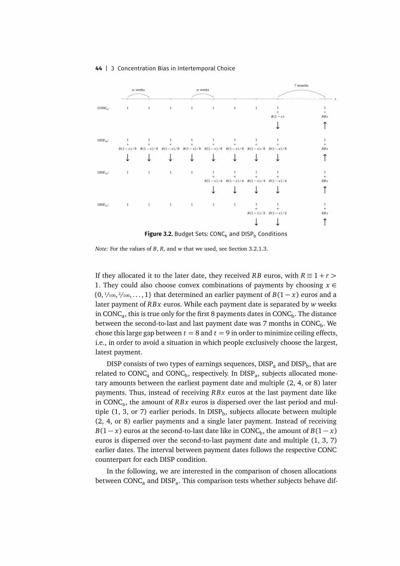
44 | 3 Concentration Bias in Intertemporal Choice
t
w weeks w weeks7 months
CONCb: 1 1 1 1 1 1 1 1+
B(1− x)
↓
1+
RBx
↑
DISPb8: 1+
B(1− x) /8
↓
1+
B(1− x) /8
↓
1+
B(1− x) /8
↓
1+
B(1− x) /8
↓
1+
B(1− x) /8
↓
1+
B(1− x) /8
↓
1+
B(1− x) /8
↓
1+
B(1− x) /8
↓
1+
RBx
↑
DISPb4: 1 1 1 1 1+
B(1− x) /4
↓
1+
B(1− x) /4
↓
1+
B(1− x) /4
↓
1+
B(1− x) /4
↓
1+
RBx
↑
DISPb2: 1 1 1 1 1 1 1+
B(1− x) /2
↓
1+
B(1− x) /2
↓
1+
RBx
↑Figure 3.2. Budget Sets: CONCb and DISPb Conditions
Note: For the values of B, R, and w that we used, see Section 3.2.1.3.
If they allocated it to the later date, they received RB euros, with R≡ 1+ r >1. They could also choose convex combinations of payments by choosing x ∈{0, 1/100, 2/100, . . . , 1} that determined an earlier payment of B(1− x) euros and alater payment of RBx euros. While each payment date is separated by w weeksin CONCa, this is true only for the first 8 payments dates in CONCb. The distancebetween the second-to-last and last payment date was 7 months in CONCb. Wechose this large gap between t = 8 and t = 9 in order to minimize ceiling effects,i.e., in order to avoid a situation in which people exclusively choose the largest,latest payment.
DISP consists of two types of earnings sequences, DISPa and DISPb, that arerelated to CONCa and CONCb, respectively. In DISPa, subjects allocated mone-tary amounts between the earliest payment date and multiple (2, 4, or 8) laterpayments. Thus, instead of receiving RBx euros at the last payment date likein CONCa, the amount of RBx euros is dispersed over the last period and mul-tiple (1, 3, or 7) earlier periods. In DISPb, subjects allocate between multiple(2, 4, or 8) earlier payments and a single later payment. Instead of receivingB(1− x) euros at the second-to-last date like in CONCb, the amount of B(1− x)euros is dispersed over the second-to-last payment date and multiple (1, 3, 7)earlier dates. The interval between payment dates follows the respective CONCcounterpart for each DISP condition.
In the following, we are interested in the comparison of chosen allocationsbetween CONCa and DISPa. This comparison tests whether subjects behave dif-
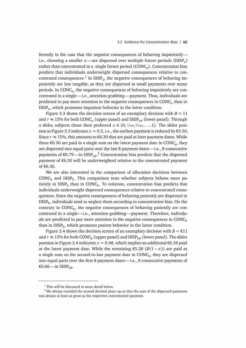
3.2 Evidence for Concentration Bias | 45
ferently in the case that the negative consequences of behaving impatiently—i.e., choosing a smaller x—are dispersed over multiple future periods (DISPa)rather than concentrated in a single future period (CONCa). Concentration biaspredicts that individuals underweight dispersed consequences relative to con-centrated consequences.1 In DISPa, the negative consequences of behaving im-patiently are less tangible, as they are dispersed in small payments over manyperiods. In CONCa, the negative consequences of behaving impatiently are con-centrated in a single—i.e., attention-grabbing—payment. Thus, individuals arepredicted to pay more attention to the negative consequences in CONCa than inDISPa, which promotes impatient behavior in the latter condition.
Figure 3.3 shows the decision screen of an exemplary decision with B = 11and r ≈ 15% for both CONCa (upper panel) and DISPa8 (lower panel). Througha slider, subjects chose their preferred x ∈ {0, 1/100, 2/100, . . . , 1}. The slider posi-tion in Figure 3.3 indicates x = 0.5, i.e., the earliest payment is reduced by €5.50.Since r ≈ 15%, this amounts to €6.30 that are paid at later payment dates. Whilethese €6.30 are paid in a single sum on the latest payment date in CONCa, theyare dispersed into equal parts over the last 8 payment dates—i.e., 8 consecutivepayments of €0.79—in DISPa8.
2 Concentration bias predicts that the dispersedpayment of €6.30 will be underweighted relative to the concentrated paymentof €6.30.
We are also interested in the comparison of allocation decisions betweenCONCb and DISPb. This comparison tests whether subjects behave more pa-tiently in DISPb than in CONCb. To reiterate, concentration bias predicts thatindividuals underweight dispersed consequences relative to concentrated conse-quences. Since the negative consequences of behaving patiently are dispersed inDISPb, individuals tend to neglect them according to concentration bias. On thecontrary in CONCb, the negative consequences of behaving patiently are con-centrated in a single—i.e., attention-grabbing—payment. Therefore, individu-als are predicted to pay more attention to the negative consequences in CONCb
than in DISPb, which promotes patient behavior in the latter condition.Figure 3.4 shows the decision screen of an exemplary decision with B = €11
and r ≈ 15% for both CONCb (upper panel) and DISPb8 (lower panel). The sliderposition in Figure 3.4 indicates x = 0.48, which implies an additional €6.56 paidat the latest payment date. While the remaining €5.28 (B(1− x)) are paid asa single sum on the second-to-last payment date in CONCb, they are dispersedinto equal parts over the first 8 payment dates—i.e., 8 consecutive payments of€0.66—in DISPb8.
1 This will be discussed in more detail below.2We always rounded the second decimal place up so that the sum of the dispersed payments
was always at least as great as the respective concentrated payment.
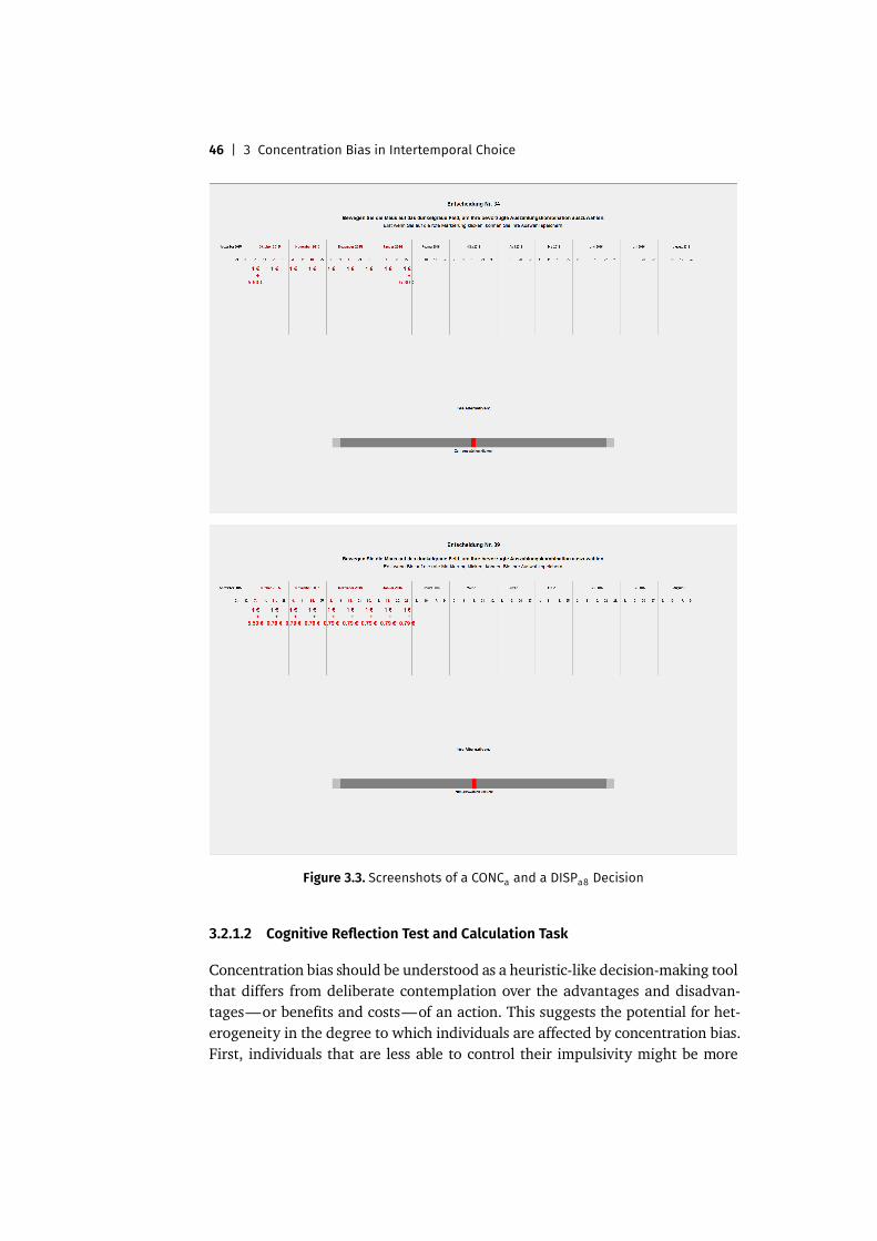
46 | 3 Concentration Bias in Intertemporal Choice
Figure 3.3. Screenshots of a CONCa and a DISPa8 Decision
3.2.1.2 Cognitive Reflection Test and Calculation Task
Concentration bias should be understood as a heuristic-like decision-making toolthat differs from deliberate contemplation over the advantages and disadvan-tages—or benefits and costs—of an action. This suggests the potential for het-erogeneity in the degree to which individuals are affected by concentration bias.First, individuals that are less able to control their impulsivity might be more
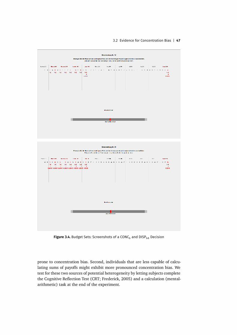
3.2 Evidence for Concentration Bias | 47
Figure 3.4. Budget Sets: Screenshots of a CONCb and DISPb8 Decision
prone to concentration bias. Second, individuals that are less capable of calcu-lating sums of payoffs might exhibit more pronounced concentration bias. Wetest for these two sources of potential heterogeneity by letting subjects completethe Cognitive Reflection Test (CRT; Frederick, 2005) and a calculation (mental-arithmetic) task at the end of the experiment.
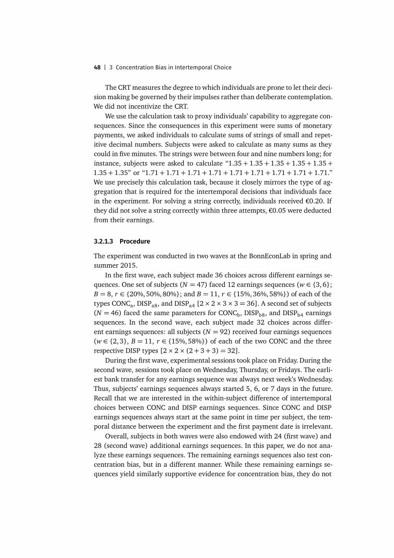
48 | 3 Concentration Bias in Intertemporal Choice
The CRTmeasures the degree to which individuals are prone to let their deci-sion making be governed by their impulses rather than deliberate contemplation.We did not incentivize the CRT.
We use the calculation task to proxy individuals’ capability to aggregate con-sequences. Since the consequences in this experiment were sums of monetarypayments, we asked individuals to calculate sums of strings of small and repet-itive decimal numbers. Subjects were asked to calculate as many sums as theycould in five minutes. The strings were between four and nine numbers long; forinstance, subjects were asked to calculate “1.35+ 1.35+ 1.35+ 1.35+ 1.35+1.35+ 1.35” or “1.71+ 1.71+ 1.71+ 1.71+ 1.71+ 1.71+ 1.71+ 1.71+ 1.71.”We use precisely this calculation task, because it closely mirrors the type of ag-gregation that is required for the intertemporal decisions that individuals facein the experiment. For solving a string correctly, individuals received €0.20. Ifthey did not solve a string correctly within three attempts, €0.05 were deductedfrom their earnings.
3.2.1.3 Procedure
The experiment was conducted in two waves at the BonnEconLab in spring andsummer 2015.
In the first wave, each subject made 36 choices across different earnings se-quences. One set of subjects (N = 47) faced 12 earnings sequences (w ∈ {3, 6};B = 8, r ∈ {20%,50%, 80%}; and B = 11, r ∈ {15%,36%, 58%}) of each of thetypes CONCa, DISPa8, and DISPa4 [2× 2× 3× 3= 36]. A second set of subjects(N = 46) faced the same parameters for CONCb, DISPb8, and DISPb4 earningssequences. In the second wave, each subject made 32 choices across differ-ent earnings sequences: all subjects (N = 92) received four earnings sequences(w ∈ {2, 3}, B = 11, r ∈ {15%,58%}) of each of the two CONC and the threerespective DISP types [2× 2× (2+ 3+ 3)= 32].
During the first wave, experimental sessions took place on Friday. During thesecond wave, sessions took place on Wednesday, Thursday, or Fridays. The earli-est bank transfer for any earnings sequence was always next week’s Wednesday.Thus, subjects’ earnings sequences always started 5, 6, or 7 days in the future.Recall that we are interested in the within-subject difference of intertemporalchoices between CONC and DISP earnings sequences. Since CONC and DISPearnings sequences always start at the same point in time per subject, the tem-poral distance between the experiment and the first payment date is irrelevant.
Overall, subjects in both waves were also endowed with 24 (first wave) and28 (second wave) additional earnings sequences. In this paper, we do not ana-lyze these earnings sequences. The remaining earnings sequences also test con-centration bias, but in a different manner. While these remaining earnings se-quences yield similarly supportive evidence for concentration bias, they do not
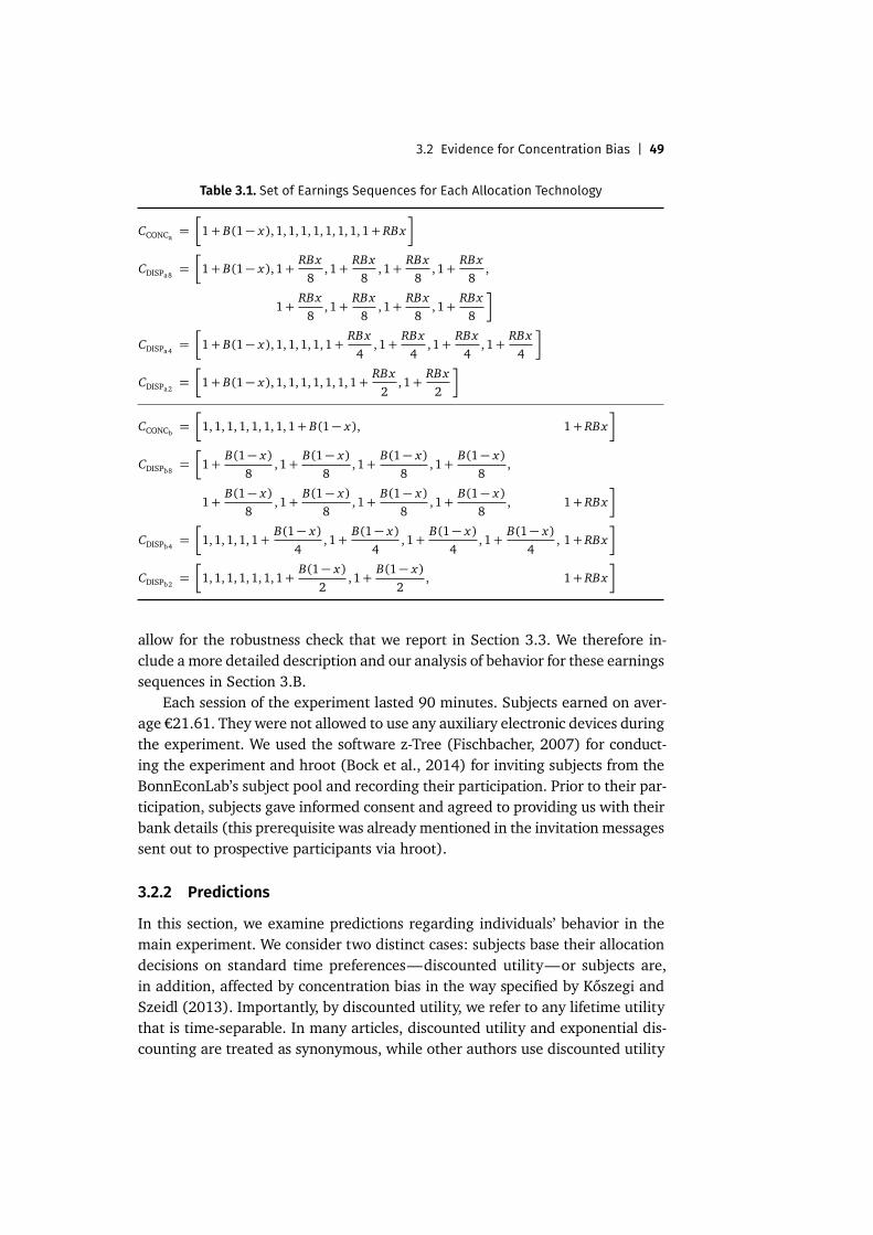
3.2 Evidence for Concentration Bias | 49
Table 3.1. Set of Earnings Sequences for Each Allocation Technology
CCONCa =�
1+ B(1− x), 1, 1, 1, 1, 1, 1, 1, 1+ RBx�
CDISPa8 =�
1+ B(1− x), 1+RBx
8,1+
RBx8
, 1+RBx
8, 1+
RBx8
,
1+RBx
8,1+
RBx8
, 1+RBx
8, 1+
RBx8
�
CDISPa4 =�
1+ B(1− x), 1, 1, 1, 1, 1+RBx
4, 1+
RBx4
,1+RBx
4,1+
RBx4
�
CDISPa2 =�
1+ B(1− x), 1, 1, 1, 1, 1, 1, 1+RBx
2,1+
RBx2
�
CCONCb =�
1,1, 1,1, 1,1, 1,1+ B(1− x), 1+ RBx�
CDISPb8 =�
1+B(1− x)
8,1+
B(1− x)8
, 1+B(1− x)
8, 1+
B(1− x)8
,
1+B(1− x)
8,1+
B(1− x)8
, 1+B(1− x)
8, 1+
B(1− x)8
, 1+ RBx�
CDISPb4 =�
1,1, 1,1, 1+B(1− x)
4, 1+
B(1− x)4
,1+B(1− x)
4,1+
B(1− x)4
, 1+ RBx�
CDISPb2 =�
1,1, 1,1, 1,1, 1+B(1− x)
2,1+
B(1− x)2
, 1+ RBx�
allow for the robustness check that we report in Section 3.3. We therefore in-clude a more detailed description and our analysis of behavior for these earningssequences in Section 3.B.
Each session of the experiment lasted 90 minutes. Subjects earned on aver-age €21.61. They were not allowed to use any auxiliary electronic devices duringthe experiment. We used the software z-Tree (Fischbacher, 2007) for conduct-ing the experiment and hroot (Bock et al., 2014) for inviting subjects from theBonnEconLab’s subject pool and recording their participation. Prior to their par-ticipation, subjects gave informed consent and agreed to providing us with theirbank details (this prerequisite was already mentioned in the invitation messagessent out to prospective participants via hroot).
3.2.2 Predictions
In this section, we examine predictions regarding individuals’ behavior in themain experiment. We consider two distinct cases: subjects base their allocationdecisions on standard time preferences—discounted utility—or subjects are,in addition, affected by concentration bias in the way specified by Kőszegi andSzeidl (2013). Importantly, by discounted utility, we refer to any lifetime utilitythat is time-separable. In many articles, discounted utility and exponential dis-counting are treated as synonymous, while other authors use discounted utility
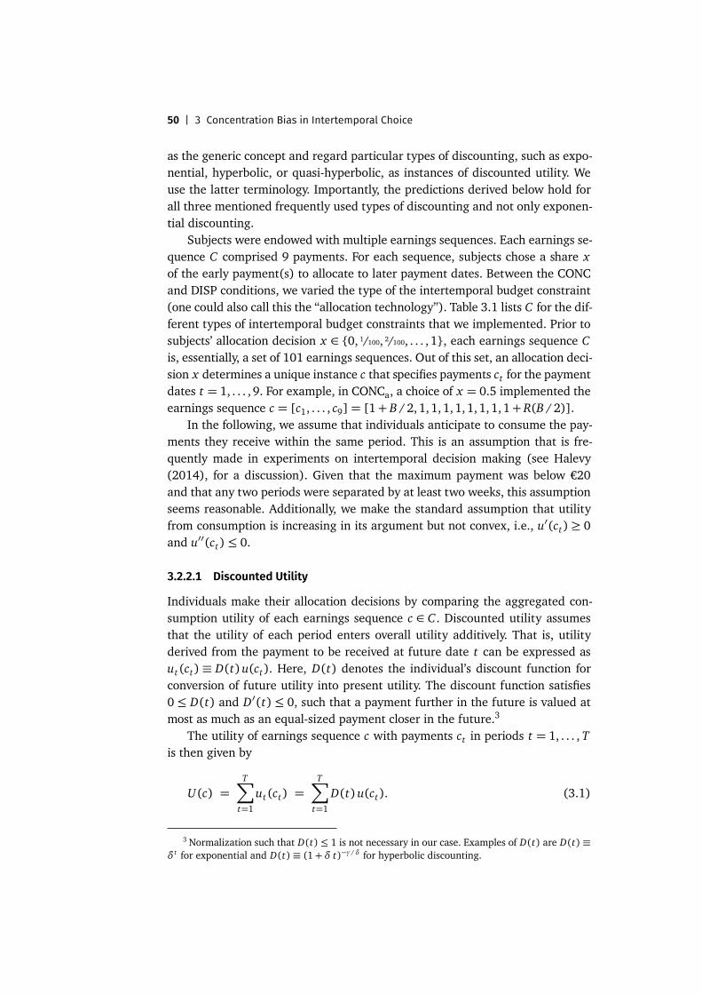
50 | 3 Concentration Bias in Intertemporal Choice
as the generic concept and regard particular types of discounting, such as expo-nential, hyperbolic, or quasi-hyperbolic, as instances of discounted utility. Weuse the latter terminology. Importantly, the predictions derived below hold forall three mentioned frequently used types of discounting and not only exponen-tial discounting.
Subjects were endowed with multiple earnings sequences. Each earnings se-quence C comprised 9 payments. For each sequence, subjects chose a share xof the early payment(s) to allocate to later payment dates. Between the CONCand DISP conditions, we varied the type of the intertemporal budget constraint(one could also call this the “allocation technology”). Table 3.1 lists C for the dif-ferent types of intertemporal budget constraints that we implemented. Prior tosubjects’ allocation decision x ∈ {0, 1/100, 2/100, . . . , 1}, each earnings sequence Cis, essentially, a set of 101 earnings sequences. Out of this set, an allocation deci-sion x determines a unique instance c that specifies payments ct for the paymentdates t = 1, . . . , 9. For example, in CONCa, a choice of x = 0.5 implemented theearnings sequence c = [c1, . . . , c9]= [1+ B /2, 1,1, 1,1, 1,1, 1,1+ R(B /2)].
In the following, we assume that individuals anticipate to consume the pay-ments they receive within the same period. This is an assumption that is fre-quently made in experiments on intertemporal decision making (see Halevy(2014), for a discussion). Given that the maximum payment was below €20and that any two periods were separated by at least two weeks, this assumptionseems reasonable. Additionally, we make the standard assumption that utilityfrom consumption is increasing in its argument but not convex, i.e., u′(ct)≥ 0and u′′(ct)≤ 0.
3.2.2.1 Discounted Utility
Individuals make their allocation decisions by comparing the aggregated con-sumption utility of each earnings sequence c ∈ C . Discounted utility assumesthat the utility of each period enters overall utility additively. That is, utilityderived from the payment to be received at future date t can be expressed asut(ct)≡ D(t)u(ct). Here, D(t) denotes the individual’s discount function forconversion of future utility into present utility. The discount function satisfies0≤ D(t) and D′(t)≤ 0, such that a payment further in the future is valued atmost as much as an equal-sized payment closer in the future.3
The utility of earnings sequence c with payments ct in periods t = 1, . . . , Tis then given by
U(c) =T∑
t=1
ut(ct) =T∑
t=1
D(t)u(ct). (3.1)
3Normalization such that D(t)≤ 1 is not necessary in our case. Examples of D(t) are D(t)≡δt for exponential and D(t)≡ (1+δ t)−γ/δ for hyperbolic discounting.
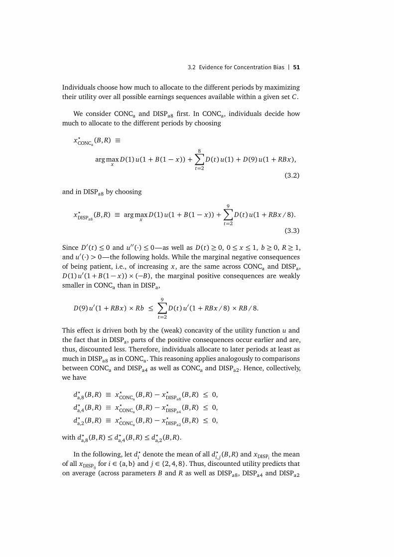
3.2 Evidence for Concentration Bias | 51
Individuals choose how much to allocate to the different periods by maximizingtheir utility over all possible earnings sequences available within a given set C .
We consider CONCa and DISPa8 first. In CONCa, individuals decide howmuch to allocate to the different periods by choosing
x?CONCa(B, R) ≡
argmaxx
D(1)u(1 + B(1 − x)) +8∑
t=2
D(t)u(1) + D(9)u(1 + RBx),
(3.2)
and in DISPa8 by choosing
x?DISPa8(B, R) ≡ arg maxx
D(1)u(1 + B(1 − x)) +9∑
t=2
D(t)u(1 + RBx /8).
(3.3)
Since D′(t)≤ 0 and u′′(·)≤ 0—as well as D(t)≥ 0, 0≤ x ≤ 1, b ≥ 0, R≥ 1,and u′(·)> 0—the following holds. While the marginal negative consequencesof being patient, i.e., of increasing x , are the same across CONCa and DISPa,D(1)u′(1+ B(1− x))× (−B), the marginal positive consequences are weaklysmaller in CONCa than in DISPa,
D(9)u′(1 + RBx) × Rb ≤9∑
t=2
D(t)u′(1 + RBx /8) × RB /8.
This effect is driven both by the (weak) concavity of the utility function u andthe fact that in DISPa, parts of the positive consequences occur earlier and are,thus, discounted less. Therefore, individuals allocate to later periods at least asmuch in DISPa8 as in CONCa. This reasoning applies analogously to comparisonsbetween CONCa and DISPa4 as well as CONCa and DISPa2. Hence, collectively,we have
d?a,8(B, R) ≡ x?CONCa(B, R) − x?DISPa8(B, R) ≤ 0,
d?a,4(B, R) ≡ x?CONCa(B, R) − x?DISPa4(B, R) ≤ 0,
d?a,2(B, R) ≡ x?CONCa(B, R) − x?DISPa2(B, R) ≤ 0,
with d?a,8(B, R)≤ d?a,4(B, R)≤ d?a,2(B, R).
In the following, let d?i denote the mean of all d?i, j(B, R) and xDISPi the meanof all xDISPij for i ∈ {a,b} and j ∈ {2,4, 8}. Thus, discounted utility predicts thaton average (across parameters B and R as well as DISPa8, DISPa4 and DISPa2
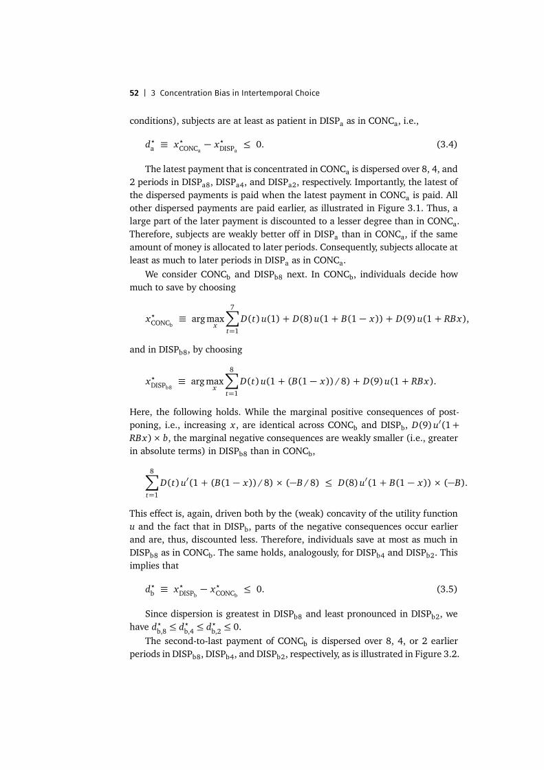
52 | 3 Concentration Bias in Intertemporal Choice
conditions), subjects are at least as patient in DISPa as in CONCa, i.e.,
d?a ≡ x?CONCa− x?DISPa ≤ 0. (3.4)
The latest payment that is concentrated in CONCa is dispersed over 8, 4, and2 periods in DISPa8, DISPa4, and DISPa2, respectively. Importantly, the latest ofthe dispersed payments is paid when the latest payment in CONCa is paid. Allother dispersed payments are paid earlier, as illustrated in Figure 3.1. Thus, alarge part of the later payment is discounted to a lesser degree than in CONCa.Therefore, subjects are weakly better off in DISPa than in CONCa, if the sameamount of money is allocated to later periods. Consequently, subjects allocate atleast as much to later periods in DISPa as in CONCa.
We consider CONCb and DISPb8 next. In CONCb, individuals decide howmuch to save by choosing
x?CONCb≡ arg max
x
7∑
t=1
D(t)u(1) + D(8)u(1 + B(1 − x)) + D(9)u(1 + RBx),
and in DISPb8, by choosing
x?DISPb8 ≡ arg maxx
8∑
t=1
D(t)u(1 + (B(1 − x)) /8) + D(9)u(1 + RBx).
Here, the following holds. While the marginal positive consequences of post-poning, i.e., increasing x , are identical across CONCb and DISPb, D(9)u′(1+RBx)× b, the marginal negative consequences are weakly smaller (i.e., greaterin absolute terms) in DISPb8 than in CONCb,
8∑
t=1
D(t)u′(1 + (B(1 − x)) /8) × (−B /8) ≤ D(8)u′(1 + B(1 − x)) × (−B).
This effect is, again, driven both by the (weak) concavity of the utility functionu and the fact that in DISPb, parts of the negative consequences occur earlierand are, thus, discounted less. Therefore, individuals save at most as much inDISPb8 as in CONCb. The same holds, analogously, for DISPb4 and DISPb2. Thisimplies that
d?b ≡ x?DISPb − x?CONCb≤ 0. (3.5)
Since dispersion is greatest in DISPb8 and least pronounced in DISPb2, wehave d?b,8 ≤ d?b,4 ≤ d?b,2 ≤ 0.
The second-to-last payment of CONCb is dispersed over 8, 4, or 2 earlierperiods in DISPb8, DISPb4, and DISPb2, respectively, as is illustrated in Figure 3.2.
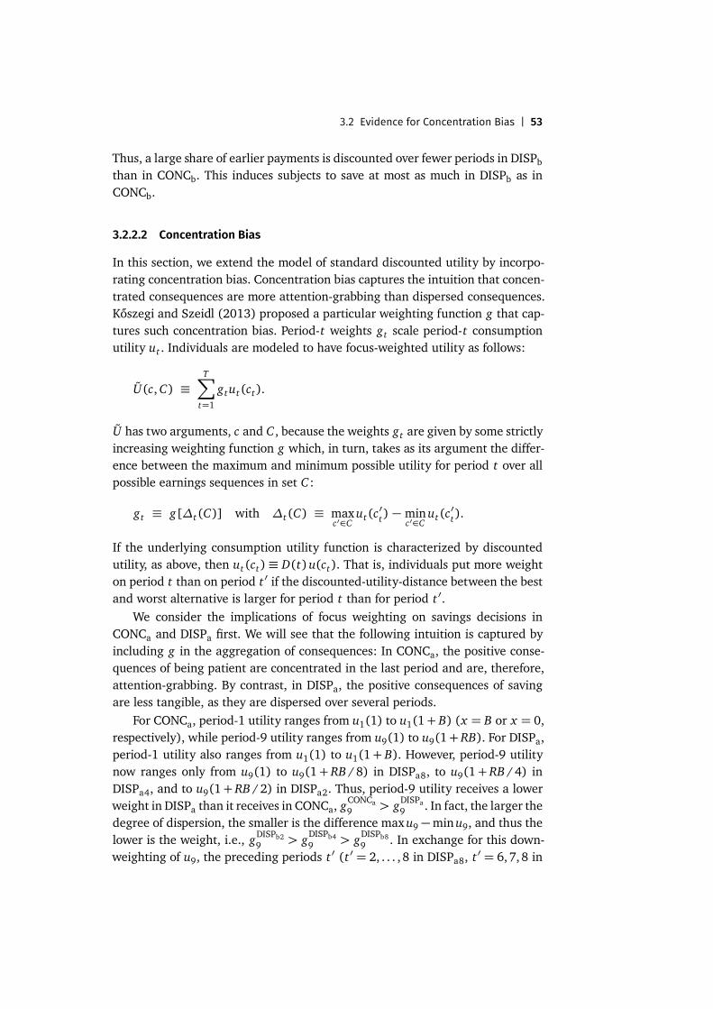
3.2 Evidence for Concentration Bias | 53
Thus, a large share of earlier payments is discounted over fewer periods in DISPbthan in CONCb. This induces subjects to save at most as much in DISPb as inCONCb.
3.2.2.2 Concentration Bias
In this section, we extend the model of standard discounted utility by incorpo-rating concentration bias. Concentration bias captures the intuition that concen-trated consequences are more attention-grabbing than dispersed consequences.Kőszegi and Szeidl (2013) proposed a particular weighting function g that cap-tures such concentration bias. Period-t weights gt scale period-t consumptionutility ut . Individuals are modeled to have focus-weighted utility as follows:
U(c, C) ≡T∑
t=1
gtut(ct).
U has two arguments, c and C , because the weights gt are given by some strictlyincreasing weighting function g which, in turn, takes as its argument the differ-ence between the maximum and minimum possible utility for period t over allpossible earnings sequences in set C :
gt ≡ g[∆t(C)] with ∆t(C) ≡ maxc′∈C
ut(c′t) − min
c′∈Cut(c
′t).
If the underlying consumption utility function is characterized by discountedutility, as above, then ut(ct)≡ D(t)u(ct). That is, individuals put more weighton period t than on period t ′ if the discounted-utility-distance between the bestand worst alternative is larger for period t than for period t ′.
We consider the implications of focus weighting on savings decisions inCONCa and DISPa first. We will see that the following intuition is captured byincluding g in the aggregation of consequences: In CONCa, the positive conse-quences of being patient are concentrated in the last period and are, therefore,attention-grabbing. By contrast, in DISPa, the positive consequences of savingare less tangible, as they are dispersed over several periods.
For CONCa, period-1 utility ranges from u1(1) to u1(1+ B) (x = B or x = 0,respectively), while period-9 utility ranges from u9(1) to u9(1+ RB). For DISPa,period-1 utility also ranges from u1(1) to u1(1+ B). However, period-9 utilitynow ranges only from u9(1) to u9(1+ RB /8) in DISPa8, to u9(1+ RB /4) inDISPa4, and to u9(1+ RB /2) in DISPa2. Thus, period-9 utility receives a lowerweight in DISPa than it receives in CONCa, gCONCa
9 > gDISPa9 . In fact, the larger the
degree of dispersion, the smaller is the difference max u9 −min u9, and thus thelower is the weight, i.e., gDISPb2
9 > gDISPb49 > gDISPb8
9 . In exchange for this down-weighting of u9, the preceding periods t ′ (t ′ = 2, . . . , 8 in DISPa8, t ′ = 6,7, 8 in

54 | 3 Concentration Bias in Intertemporal Choice
DISPa4, and t ′ = 8 in DISPa2) receive a larger weight gt ′ in DISPa than in CONCa.This is because for those periods, max ut ′ −min ut ′ = 0 in CONCa, while it is pos-itive in DISPa. Importantly, g is strictly increasing. If g is sufficiently steep, thenthe relatively large weight g9 in CONCa is greater than the sum of the multiplesmaller weights gt ′ , including g9, in DISPa.
Expressed verbally, the positive consequences of being patient are under-weighted in DISPa relative to CONCa. If this relative underweighting of dis-persed payoffs in DISPa is sufficiently strong, focus-weighted utility predictslarger marginal utility from being patient in CONCa than in DISPa. In that case,the prediction of the standard model—as specified in equation (3.4)—is re-versed: focus-weighting individuals may want to save more in CONCa than inDISPa. Let
?? indicate optimal choices according to discounted utility in combina-tion with focusing (in analogue to ? indicating optimal choices under discountedutility without focus weighting). Then we have, with a sufficiently positive slopeof the weighting function g,4
d??a ≡ x??CONCa− x??DISPa > 0 (3.6)
as well as d??a,8 ≥ d??a,4 ≥ d??a,2 > 0.We now turn to the implications of focus-weighted utility on savings deci-
sions in CONCb and DISPb. Recall that in DISPb, the negative consequences ofsaving are dispersed over several payment dates, while they are concentrated ata single, thus attention-grabbing, payment date (t = 8) in CONCb. The strictlyincreasing weighting function g captures this potential neglect of the dispersedpayoffs in DISPb. Period-8 utility ranges from u8(1) to u8(1+ B) (for x = Band x = 0, respectively) in CONCb. By contrast, it ranges only from u8(1) tou8(1+ B /8) in DISPb8, to u8(1+ B /4) in DISPb4, and to u8(1+ B /2) in DISPb2.Hence, focus-weighted utility assigns a lower weight to period-8 utility in DISPbthan in CONCb. In exchange for this downweighting of u8, the preceding periodst ′ (t ′ = 1, . . . , 7 in DISPb8, t ′ = 5, 6,7 in DISPb4, and t ′ = 7 in DISPb2) receivea larger weight gt ′ in DISPb than in CONCb. This is because for those periods,max ut ′ −min ut ′ = 0 in CONCb, while it is positive in DISPb. Just as before, if theslope of g is sufficiently positive, then the relatively large weight g8 in CONCb isgreater than the sum of the multiple smaller weights gt ′ , including g8, in DISPb.
If such underweighting of the utility generated by early payments (up to pay-ment date no. 8) is sufficiently strong in DISPb, then focus-weighting reversesthe prediction of the standard model—as stated in equation (3.5)—by predict-
4 The weighting function has to be steep enough to offset any potential effects from discount-ing, concavity of the per-period utility function, and the interest rate R that might favor thedispersed payment.
3.2 Evidence for Concentration Bias | 55
ing that individuals save more in DISPb than in CONCb:
d??b ≡ x??DISPb − x??CONCb> 0, (3.7)
and d??b,8 ≥ d??b,4 ≥ d??b,2 > 0.In the following, we compare savings decisions between CONCa and DISPa
as well as between CONCb and DISPb. We hypothesize that concentration biasis sufficiently strong and leads individuals to save more in CONCa than in DISPa,d??a > 0, as well as more in DISPb than in CONCb, d??b > 0. Both effects takentogether yield the prediction regarding the aggregated concentration bias ofd?? > 0, with d?? being the average of d??a and d??b .
Hypothesis 4. Subjects allocate more money to payments that are concentrated ata single date than to equal-sized payments that are dispersed over multiple earlierdates, d?? > 0 (in contrast to standard discounting).
Define variables d??j to capture the differences in savings averaged across thedifferent degrees of dispersion: d??j ≡ (d??a, j + d??b, j) /2 for j = 2,4, 8.
Hypothesis 5. The effect described in Hypothesis 4 is the more pronounced, themore dispersed a payment is, i.e., d??8 > d??4 > d??2 > 0.
3.2.3 Results
Subjects mademultiple allocation decisions in our experiment. In particular, sub-jects made several allocation decisions for CONC and DISP earnings sequences.This allows us to calculate for each individual the average difference of moneyallocated to later periods between CONC and DISP earnings sequences. De-note by x , d, etc. the empirical counterparts of the variables introduced in Sec-tion 3.2.2 (i.e., of x?/??, d?/??, etc.). That is, d is the individual average of da(= xCONCa
− xDISPa) and db (= xDISPb − xCONCb).
3.2.3.1 Test of Hypothesis 4
With this, we can report our first result.
Result 7. On average, subjects allocated more money to payments that were con-centrated rather than dispersed, i.e., our measure of concentration bias, d, is sig-nificantly larger than zero.
Our first result supports Hypothesis 4. Subjects allocated d = 6.3 percentagepoints (p.p.) more money into payments that were concentrated rather thandispersed. This treatment effect is statistically significant, suing a t-test, withstandard errors corrected for potential clustering on the subject level (see Ta-
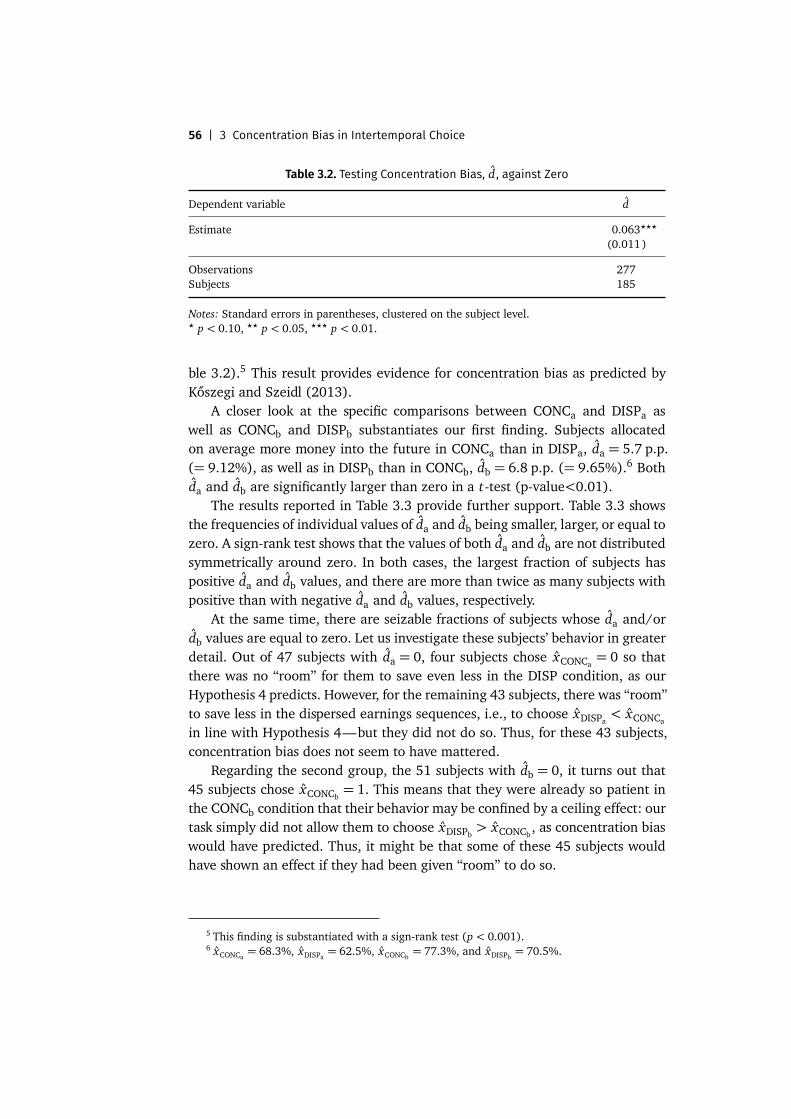
56 | 3 Concentration Bias in Intertemporal Choice
Table 3.2. Testing Concentration Bias, d , against Zero
Dependent variable d
Estimate 0.063???
(0.011)
Observations 277Subjects 185
Notes: Standard errors in parentheses, clustered on the subject level.? p < 0.10, ?? p < 0.05, ??? p < 0.01.
ble 3.2).5 This result provides evidence for concentration bias as predicted byKőszegi and Szeidl (2013).
A closer look at the specific comparisons between CONCa and DISPa aswell as CONCb and DISPb substantiates our first finding. Subjects allocatedon average more money into the future in CONCa than in DISPa, da = 5.7 p.p.(= 9.12%), as well as in DISPb than in CONCb, db = 6.8 p.p. (= 9.65%).6 Bothda and db are significantly larger than zero in a t-test (p-value<0.01).
The results reported in Table 3.3 provide further support. Table 3.3 showsthe frequencies of individual values of da and db being smaller, larger, or equal tozero. A sign-rank test shows that the values of both da and db are not distributedsymmetrically around zero. In both cases, the largest fraction of subjects haspositive da and db values, and there are more than twice as many subjects withpositive than with negative da and db values, respectively.
At the same time, there are seizable fractions of subjects whose da and/ordb values are equal to zero. Let us investigate these subjects’ behavior in greaterdetail. Out of 47 subjects with da = 0, four subjects chose xCONCa
= 0 so thatthere was no “room” for them to save even less in the DISP condition, as ourHypothesis 4 predicts. However, for the remaining 43 subjects, there was “room”to save less in the dispersed earnings sequences, i.e., to choose xDISPa < xCONCa
in line with Hypothesis 4—but they did not do so. Thus, for these 43 subjects,concentration bias does not seem to have mattered.
Regarding the second group, the 51 subjects with db = 0, it turns out that45 subjects chose xCONCb
= 1. This means that they were already so patient inthe CONCb condition that their behavior may be confined by a ceiling effect: ourtask simply did not allow them to choose xDISPb > xCONCb
, as concentration biaswould have predicted. Thus, it might be that some of these 45 subjects wouldhave shown an effect if they had been given “room” to do so.
5 This finding is substantiated with a sign-rank test (p < 0.001).6 xCONCa = 68.3%, xDISPa = 62.5%, xCONCb = 77.3%, and xDISPb = 70.5%.
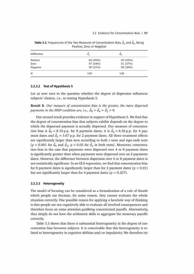
3.2 Evidence for Concentration Bias | 57
Table 3.3. Frequencies of the Two Measures of Concentration Bias, da and db, BeingPositive, Zero, or Negative
Difference da db
Positive 63 (45%) 59 (43%)Zero 47 (34%) 51 (37%)Negative 29 (21%) 28 (20%)
N 139 138
3.2.3.2 Test of Hypothesis 5
Let us now turn to the question whether the degree of dispersion influencessubjects’ choices, i.e., to testing Hypothesis 5.
Result 8. Our measure of concentration bias is the greater, the more dispersedpayments in the DISP condition are, i.e., d8 > d4 > d2 > 0.
Our second result provides evidence in support of Hypothesis 5. We find thatthe degree of concentration bias that subjects exhibit depends on the degree towhich the dispersed payment is actually dispersed. Our measure of concentra-tion bias is d8 = 8.10 p.p. for 8 payment dates; it is d4 = 6.56 p.p. for 4 pay-ment dates and d2 = 3.67 p.p. for 2 payment dates. All three treatment effectsare significantly larger than zero according to both t-tests and sign-rank tests(p < 0.001 for d8 and d4; p < 0.05 for d2 in both tests). Moreover, concentra-tion bias in the case that payments were dispersed over 4 or 8 payment datesis significantly greater than when payments were dispersed over on 2 paymentsdates. However, the difference between dispersion over 4 or 8 payment dates isnot statistically significant: In an OLS regression, we find that concentration biasfor 8 payment dates is significantly larger than for 2 payment dates (p < 0.01)but not significantly larger than for 4 payment dates (p = 0.237).
3.2.3.3 Heterogeneity
The model of focusing can be considered as a formalization of a rule of thumbwhich people use because, for some reason, they cannot evaluate the wholesituation correctly. One possible reason for applying a heuristic way of thinkingis that people are not cognitively able to evaluate all involved consequences andtherefore focus on some attention-grabbing concentrated payoffs. Alternatively,they simply do not have the arithmetic skills to aggregate the monetary payoffscorrectly.
Table 3.3 shows that there is substantial heterogeneity in the degree of con-centration bias between subjects. It is conceivable that this heterogeneity is re-lated to heterogeneity in cognitive abilities and/or impulsivity. We therefore try
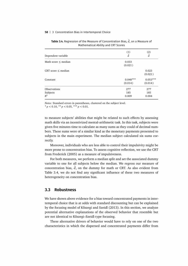
58 | 3 Concentration Bias in Intertemporal Choice
Table 3.4. Regression of the Measure of Concentration Bias, d , on a Measure ofMathematical Ability and CRT Scores
(1) (2)Dependent variable d d
Math score ≤ median 0.033(0.021)
CRT score ≤ median 0.023(0.021)
Constant 0.048??? 0.053???
(0.014) (0.014)
Observations 277 277Subjects 185 185R2 0.009 0.004
Notes: Standard errors in parentheses, clustered on the subject level.? p < 0.10, ?? p < 0.05, ??? p < 0.01.
to measure subjects’ abilities that might be related to such effects by assessingmath skills via an incentivized mental-arithmetic task. In this task, subjects weregiven five minutes time to calculate as many sums as they could of decimal num-bers. These sums were of a similar kind as the monetary payments presented tosubjects in the main experiment. The median subject calculated six sums cor-rectly.
Moreover, individuals who are less able to control their impulsivity might bemore prone to concentration bias. To assess cognitive reflection, we use the CRTfrom Frederick (2005) as a measure of impulsiveness.
For both measures, we perform a median split and set the associated dummyvariable to one for all subjects below the median. We regress our measure ofconcentration bias, d, on the dummy for math or CRT. As also evident fromTable 3.4, we do not find any significant influence of these two measures ofheterogeneity on concentration bias.
3.3 Robustness
We have shown above evidence for a bias toward concentrated payments in inter-temporal choice that is at odds with standard discounting but can be explainedby the focusing model of Kőszegi and Szeidl (2013). In this section, we analyzepotential alternative explanations of the observed behavior that resemble butare not identical to Kőszegi–Szeidl-type focusing.
These alternative drivers of behavior would have to rely on one of the twocharacteristics in which the dispersed and concentrated payments differ from
3.3 Robustness | 59
each other: First, it might be the case that subjects are averse against small pay-ments. For instance, subjects may have a distaste against receiving lots of change(i.e., small coins) rather than bills. While a distaste against small paymentsshould not matter in the context of our experiment as payments are conductedthough bank transfers, we cannot rule out that subjects feel this way. Second, thecomputational complexity of evaluating an earnings sequence is greater when itincludes dispersed and not only concentrated payments. This greater computa-tional complexity may cause errors in subjects’ calculations. White-noise errorswould only result in inconsistent choices but not in a preference for concentratedpayments. However, it is conceivable for our task that these mathematical errorsare systematic in the direction of “subadditivity”—meaning that people calcu-late the sum of the dispersed payments to be too small.7 As a consequence, sub-jects would undervalue dispersed payments vis-à-vis concentrated sequences.
To control for these two potential effects, we made use of a control exper-iment in which all dispersed payments were “dispersed within a day” and notover different payment dates. Recall that the last bank transfer of a dispersedpayment in DISPa and DISPb is always completed at the same date as the respec-tive concentrated payment in CONCa and CONCb. In our “dispersedwithin a day”control experiment, we therefore mirrored the combined features of the DISPand CONC conditions: we made the dispersed payments de facto identical to theconcentrated ones, by scheduling all “dispersed” payments on the date of theconcentrated payment. In other words, the “dispersed within a day” paymentsare completely equivalent to the concentrated payments except the differencein the display: subjects saw 2, 4, or 8 relatively small monetary amounts thatthey would have to add to calculate the total earnings that they would receive atthat date. Figure 3.5 displays a screenshot of the graphical representation thatwas shown to subjects who participated in this control experiment.
Overall, subjects in the control experiment made the same amount of al-location decisions as subjects in the main experiment did. The only differencebetween these decisions was that in the main experiment DISP-type allocationdecisions concern dispersion over multiple payment dates, while in the controlexperiment DISP-type allocation decisions concern dispersion within a paymentdate, as explained above. Thus, we can calculated the same average differenceof money allocated to “concentrated”—or not dispersed—payments, i.e., d, forsubjects in the control experiment as we did for subjects of the main experiment.
7 There is evidence that people suffer from “left-digit bias”—a “tendency to focus on the left-most digit of a number while partially ignoring other digits”—even in situations in which theyhave monetary incentives to overcome such bias (Lacetera et al., 2012). A left-digit bias couldlead to undervaluation of dispersed compared to concentrated payoffs in our experiment. Onemight argue that left-digit bias is a potential “micro-foundation” of Kőszegi and Szeidl’s (2013)focus weights; however, one might also view left-digit bias and resulting undervaluation of a sumas a mathematical error that should be ruled out as an explanation.
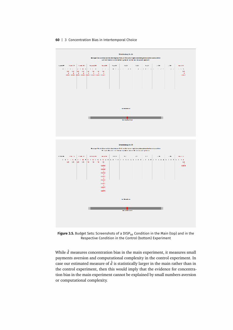
60 | 3 Concentration Bias in Intertemporal Choice
Figure 3.5. Budget Sets: Screenshots of a DISPb8 Condition in the Main (top) and in theRespective Condition in the Control (bottom) Experiment
While d measures concentration bias in the main experiment, it measures smallpayments aversion and computational complexity in the control experiment. Incase our estimated measure of d is statistically larger in the main rather than inthe control experiment, then this would imply that the evidence for concentra-tion bias in the main experiment cannot be explained by small numbers aversionor computational complexity.
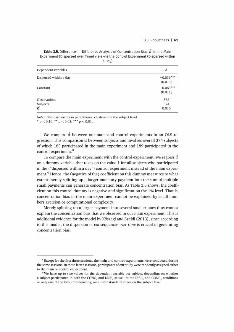
3.3 Robustness | 61
Table 3.5. Difference-in-Difference Analysis of Concentration Bias, d , in the MainExperiment (Dispersed over Time) vis-à-vis the Control Experiment (Dispersed within
a Day)
Dependent variables d
Dispersed within a day −0.036???
(0.013)
Constant 0.063???
(0.011)
Observations 562Subjects 374R2 0.016
Notes: Standard errors in parentheses, clustered on the subject level.? p < 0.10, ?? p < 0.05, ??? p < 0.01.
We compare d between our main and control experiments in an OLS re-gression. This comparison is between subjects and involves overall 374 subjectsof which 185 participated in the main experiment and 189 participated in thecontrol experiment.8
To compare the main experiment with the control experiment, we regress don a dummy variable that takes on the value 1 for all subjects who participatedin the (“dispersed within a day”) control experiment instead of the main experi-ment.9 Hence, the (negative of the) coefficient on this dummy measures to whatextent merely splitting up a larger monetary payment into the sum of multiplesmall payments can generate concentration bias. As Table 3.5 shows, the coeffi-cient on this control dummy is negative and significant on the 1% level. That is,concentration bias in the main experiment cannot be explained by small num-bers aversion or computational complexity.
Merely splitting up a larger payment into several smaller ones thus cannotexplain the concentration bias that we observed in our main experiment. This isadditional evidence for the model by Kőszegi and Szeidl (2013), since accordingto this model, the dispersion of consequences over time is crucial in generatingconcentration bias.
8 Except for the first three sessions, the main and control experiments were conducted duringthe same sessions. In these latter sessions, participants of our study were randomly assigned eitherto the main or control experiment.
9We have up to two values for the dependent variable per subject, depending on whethera subject participated in both the CONCa and DISPa as well as the DISPb and CONCb conditionsor only one of the two. Consequently, we cluster standard errors on the subject level.

62 | 3 Concentration Bias in Intertemporal Choice
3.4 Conclusion
This paper is the first to provide causal evidence for a bias toward concentratedpayoffs in intertemporal choice, as it is predicted by Kőszegi and Szeidl (2013).Building on the “convex budget sets” method of Andreoni and Sprenger (2012),we designed a novel choice task that implements different types of intertemporalbudget constraints. More specifically, both earlier and later benefits in this tasktake on the form of either one-time payments or payments that are dispersedover several payments dates. We used this choice task in a laboratory experi-ment to test how spreading payments over time influences people’s intertempo-ral decisions. We find that the payments’ degree of dispersion influences subjects’choices in a way that is incompatible with discounted utility but in line with con-centration bias, as the Kőszegi–Szeidl model predicts. Our findings are relevantnot only for positive economics, i.e., for understanding and forecasting people’sbehavior, but also for normative economics, as we argue below.
To academic economists as well as politicians and entrepreneurs, how peoplemake intertemporal decisions is of great interest. For instance, how people’s sav-ings respond to changes in interest rates or how their health decisions respondto tax incentives is relevant for both the insurance sector and the government.The model most widely used for analyzing intertemporal decisions is discountedutility in combination with exponential discounting. However, people’s decisionsoften seem to contradict exponential discounting. One example is low gym at-tendance (DellaVigna and Malmendier, 2006). A different example—with hugemonetary stakes—is the “annuity puzzle” (see, e.g., Yaari, 1965; Warner andPleeter, 2001; Davidoff et al., 2005; Benartzi et al., 2011). It describes the phe-nomenon that many people choose an earlier lump-sum payment over a futurerent that is paid periodically (the annuity) evenwhen the rent has a substantiallyhigher expected present value. In fact, many other decisions from everyday lifeare similar in that available options are also characterized by payoffs or coststhat are dispersed over time—such as the benefits of not smoking or paymentplans for smartphones.
Deviations from exponential discounting have frequently been interpretedas resulting from present bias, i.e., as stemming from a lack of self-control,which can be formalized via (quasi-)hyperbolic discounting (see, e.g., Laibson,1997). Recently, Kőszegi and Szeidl (2013) have offered an alternative explana-tion of the departures from exponential discounting that occur in such decisions:a bias of decision makers toward options whose consequences are concentratedin fewer periods. Unfortunately, based on empirical data from the field alone,it will be hard or even impossible to discriminate between the competing ex-planations. More concretely, the “annuity puzzle” (Benartzi et al., 2011) couldbe the product of Kőszegi–Szeidl-type focusing. However, other factors, such asuninsuredmedical expenses, bequest motives, and adverse selection (see the dis-
3.4 Conclusion | 63
cussions in Modigliani, 1986; Davidoff et al., 2005; Benartzi et al., 2011), mayalso, at least partially, explain the empirically observed low degree of annuitiza-tion. Moreover, the predictions of hyperbolic discounting and the Kőszegi–Szeidlmodel coincide regarding under-annuitization.
By providing a controlled environment in which particular motives are ruledout or at least held constant, our lab experiment allows for establishing that thedispersion of consequences indeed causally affects discounting. Our variant ofthe “convex budget set” method (Andreoni and Sprenger, 2012) implementsboth concentrated and dispersed payments. In other words, we implement dif-ferent types of intertemporal budget constraints (different types of “investmentproducts”/“savings technologies”). For paying subjects, we use forward-datedmoney transfers to their bank accounts. In the concentrated conditions (CONCa
and CONCb), each payment is transferred on a single day. In contrast, in theassociated dispersed conditions (DISPa and DISPb), parts of the payments aredispersed over several days (importantly, these are always earlier than the asso-ciated CONC payments): in DISPa, later payments are dispersed, while in DISPb,earlier payments are dispersed.
Concentration bias, as modeled by Kőszegi and Szeidl (2013), predicts thatsubjects allocate more money to future payments (save more) in CONCa thanin DISPa. Importantly, this prediction is not made by discounted-utility models(i.e., neither by exponential nor by hyperbolic discounting). Indeed, we find thatsubjects exhibit concentration bias. Thus, they violate predictions of discounted-utility models, while their decisions are compatible with the focusing modelby Kőszegi and Szeidl (2013). Via a control treatment, we show that merelysplitting up a larger payment into several smaller ones cannot explain the con-centration bias that we observed in our main experiment. This is crucial becauseaccording to Kőszegi and Szeidl (2013), it is the dispersion of consequences overtime that generates a bias toward concentration.
Our study contributes to the literature on intertemporal choice in two impor-tant ways: First, it helps explain why in recent experiments, the observed degreeof present bias and the incidence of time-inconsistent behavior are fairly low(Andreoni and Sprenger, 2012; Augenblick et al., 2015), while they are foundto be much more severe in the analysis of field data (e.g., low gym attendance,DellaVigna and Malmendier (2006); resistance to the annuitization of pensionplans, Warner and Pleeter (2001) and Davidoff et al. (2005)). Our study doesso by identifying the lack of dispersed payments in previous lab experiments asa plausible source of this discrepancy. Second, and more importantly, we findthat the dispersion of payments influences subjects’ decisions in a way capturedneither by exponential nor by (quasi-)hyperbolic discounting.
Hence, not only previous experimental studies but also theoretical accountsof discounting, except Kőszegi and Szeidl (2013), seem to have neglected an
64 | 3 Concentration Bias in Intertemporal Choice
important facet of intertemporal choice. At the same time, our findings are alsoevidence against other recent approaches such as the “model of relative thinking”by Bushong et al. (2015), since relative thinking predicts effects in the oppositedirection of the effects predicted by focusing.
We are aware of one previous study that used multiple bank transfers to re-munerate subjects: Attema et al. (2015). Attema et al. propose a highly elegantmethod of “measuring discounting without measuring utility.” Crucially, how-ever, their method relies, first, on the assumption that lifetime utility is time-separable and, second, on measuring indifference between payment streamsthat consist of dispersed payments.10 However, the focusing model predicts a vi-olation of time separability if at least one of the functions u or g is nonlinear.Furthermore, also without any reference to the focusing model, our results indi-cate limitations to Attema et al.’s approach. Given that we find that the degreeof an option’s dispersion affects expressed discounting, it is likely that the esti-mates obtained by applying Attema et al.’s method will be sensitive to the exactpayment streams employed, i.e., to both the size of the payments and their de-gree of dispersion.
Outside the laboratory, concentration bias is essential information, for in-stance, regarding the assessment of the effectiveness of policy measures. It isconceivable, for instance, that taxes on annuities are perceived as less severe bypeople than taxes on lump-sum payments or on current income. Related to this,Chetty et al. (2009) have shown that taxes of different salience affect consumerdemand to different degrees, and they also assess the consequences of this ef-fect for consumer welfare. Thus, understanding how bias toward concentrationaffects people’s intertemporal choices is equally important for both positive andnormative economics.
References
Andreoni, James and Charles Sprenger (2012): “Risk Preferences Are Not Time Prefer-ences.” American Economic Review, 102 (7), 3357–3376. [39, 41, 43, 62, 63]
Attema, Arthur E., Han Bleichrodt, Yu Gao, Zhenxing Huang, and Peter P. Wakker(2015): “Measuring Discounting without Measuring Utility.” American Economic Review(forthcoming). [42, 64]
Augenblick, Ned, Muriel Niederle, and Charles Sprenger (2015): “Working over Time: Dy-namic Inconsistency in Real Effort Tasks.” Quarterly Journal of Economics, 130 (3),1067–1115. [41, 63]
10 The basic idea of their method is intriguingly simple: If an individual is indifferent between,say, $10 today, and $10 in one year plus an additional $10 in two years, then we can measure dis-counting without having to take the utility function into account. Under exponential discountingwith an annual discount factor δ, this indifference translates to u($10)= δu($10)+δ2u($10),so that u($10) cancels out and δ can be readily calculated as the solution to 1= δ+δ2.
References | 65
Benartzi, Shlomo, Alessandro Previtero, and Richard H. Thaler (2011): “Annuitization Puz-zles.” Journal of Economic Perspectives, 25 (4), 143–164. [62, 63]
Bock, Olaf, Ingmar Baetge, and Andreas Nicklisch (2014): “hroot: Hamburg Registrationand Organization Online Tool.” European Economic Review, 71, 117–120. [49]
Bordalo, Pedro, Nicola Gennaioli, and Andrei Shleifer (2013): “Salience and ConsumerChoice Nicola Gennaioli Andrei Shleifer.” Journal of Political Economy, 121 (5), 803–843. [42]
Bushong, Benjamin, Matthew Rabin, and Joshua Schwartzstein (2015): “A Model of Rela-tive Thinking.” Working Paper. [42, 64]
Chetty, Raj, Adam Looney, and Kory Kroft (2009): “Salience and Taxation: Theory and Evi-dence.” American Economic Review, 99 (4), 1145–1177. [64]
Davidoff, Thomas, Jeffrey R. Brown, and Peter A. Diamond (2005): “Annuities and Individ-ual Welfare.” American Economic Review, 95 (5), 1573–1590. [41, 62, 63]
DellaVigna, Stefano and Ulrike Malmendier (2006): “Paying Not to Go to the Gym.” Ameri-can Economic Review, 96 (3), 694–719. [41, 62, 63]
Fischbacher, Urs (2007): “z-Tree: Zurich Toolbox for Ready-Made Economic Experiments.”Experimental Economics, 10 (2), 171–178. [49]
Frederick, Shane (2005): “Cognitive Reflection and Decision Making.” Journal of EconomicPerspectives, 19 (4), 25–42. [47, 58]
Halevy, Yoram (2014): “Some Comments on the Use of Monetary and Primary Rewards inthe Measurement of Time Preferences.” working paper. University of British Columbia.[50]
Kahneman, Daniel (2003): “A Perspective on Judgment and Choice: Mapping Bounded Ra-tionality.” American Psychologist, 58 (9), 697–720. [38]
Kőszegi, Botond and Adam Szeidl (2013): “A Model of Focusing in Economic Choice.” Quar-terly Journal of Economics, 128 (1), 53–104. [38, 41, 42, 49, 53, 56, 58, 59, 61–63, 71]
Lacetera, Nicola, DevinG. Pope, and Justin R. Sydnor (2012): “Heuristic thinking and limitedattention in the car market.” American Economic Review, 102 (5), 2206–2236. [59]
Laibson, David (1997): “Golden Eggs and Hyperbolic Discounting.”Quarterly Journal of Eco-nomics, 112 (2), 443–478. [62]
Modigliani, Franco (1986): “Life cycle, individual thrift, and the wealth of nations.” Ameri-can Economic Review, 234 (4777), 704–12. [63]
Warner, John T. and Saul Pleeter (2001): “The Personal Discount Rate: Evidence from Mili-tary Downsizing Programs.” American Economic Review, 91 (1), 33–53. [41, 62, 63]
Yaari, Menahem E. (1965): “Uncertain Lifetime, Life Insurance, and the Theory of the Con-sumer.” Review of Economic Studies, 32 (2), 137–150. [62]

66 | 3 Concentration Bias in Intertemporal Choice
Appendix 3.A Instructions
Main and Control Experiment11
Screen 1—Welcome
We would like to ask you to be quiet during the experiment and to use thecomputer only for tasks which are part of this experiment.
If you have any questions, please raise your hand. We will come to you forhelp.
Please put your cell phone into the bag at your place.
Screen 2—Information about the Procedure
Part 1In the first part of this experiment, you will gain nine €1 payments for sure,which will be transferred to your bank account at various dates in the future.Furthermore, you receive one or multiple additional payment(s) for the first partof the experiment. For the latter one you can decide by yourself when these ad-ditional payment(s) will be transferred. The following is always the case: If youchoose a later payment, you receive, in total, more money than choosingan earlier payment.
Overall you make 60 decisions about timing and amount of money of youradditional payment(s). After you have made your decisions, one decision will berandomly picked by the computer and is paid out for real. Since every decision ispicked with the same probability, it is convenient for you to make every decisionas if it were paid out for real.
Your payment for part one will be transferred to your bank account. All or-ders for transfers will be transmitted to the bank today. We will send you an e-mail with all the data transmitted to the bank, such that you can check whetherall payments are ordered correctly!
After the last transfer you will receive another e-mail which reminds you ofall different payments and dates.
If you have any question, please raise your hand. We will come to you forhelp.
Part 2In the second part of the experiment, we would like to ask you to exercise a task.You will receive money for doing this task. We will provide information aboutthe exact payment right before the beginning of the second part. Your payment
11While the text of the instructions for the main and control experiment are the same, theincome sequences displayed on the respective screens are different, as discussed in Section 3.3.

3.A Instructions | 67
for the second part is independent of the payment for the first part and you willget paid in cash at the end of the experiment.
Screen 3
Here subjects have to enter their banking data.
Screen 4—Choice Lists12
Part 1aIn the first 24 decisions, you have to choose your most preferred option outof nine possible payment-alternatives. In all of these decisions, you have thepossibility to receive your whole payment earlier in time or, alternatively, intotal more money later in time.
In the following, before the experiment starts, we show you two possiblepayment-alternatives of a decision such that you get familiar with the decisionscreens of this experiment.
Screen 5—Example 1
In this example, the first alternative has been chosen. The slider is positionedin a way that payment-alternative 1 is displayed. In this example, payment-alternative 1 corresponds to a payment of €8 at the earliest possible date. Addi-tionally, €1 is transferred to your bank account at nine different dates.
Screen 6—Example 2
In this example, the sixth alternative has been chosen. The slider is positionedin a way that payment-alternative 6 is displayed. In this example, payment-alternative 6 corresponds to a multiple payment of €1.50 at each highlighteddate. Additionally, €1 is transferred to your bank account at nine different dates.
Screen 7—Example 3
You can choose your preferred option out of nine alternatives. All alternativesdistinguish themselves in the total amount of money and the points in timewhere transfers are realised. The following is always the case: If you choosea later payment, you receive, in total, more money than choosing an earlierpayment.
At the next screen, all nine payment-alternatives of this decision are shownin an animation.
The transfer dates are highlighted in red.
12We analyze the intertemporal decisions with respect to the the choice lists in Section 3.B.

68 | 3 Concentration Bias in Intertemporal Choice
After the animation you have the possibility to have another look at allpayment-alternatives and you can choose your most preferred alternative.
This hint will be shown for the first four decisions.
Screen 8—Budget Sets13
In part 1b you have to make 36 decisions.In each decision you have the possibility to divide a certain amount of money
between earlier and later dates. The less money you allocate to earlier dates,the more money you receive later. In other words, the total amount of moneyreceived is higher when a bigger part is allocated to later dates.
You make the decisions by using a slider with your mouse.You can practice the use of the slider:You move a red marker by moving your mouse over the dark-grey bar (do
not click!). If you click at the red marker, your choice is loged and can be savedafterwards. There will appear a red Button “Save choice!”. After clicking thisbutton, your current choice is saved.
If you want to correct a loged choice, click at the red marker again and movethe mouse to your preferred position.
Screen 9—End of Part 1
This was the last decision of the first part of the experiment.Before you learn which decision from the first part will be paid out for real,
we would like to ask you to take part in the second part of the experiment.Please click on the button “Continue.”
Screen 10—Part 2
In this part we would like to ask you to add up figures as often as you canmanage.
You have 5 minutes time for exercising this task.You receive a base payment of €1 for this part.The more numbers you can sum up correctly, the more money you can gain:
You receive €0.20 for each correct summation.You have three attempts for each summation. If you are not able to calculate
the sum correctly in the third attempt, you lose €0.05.(Attention: You have to use a period (.) instead of a comma (,) when writing
decimal numbers.)
13We analyze the intertemporal decisions with respect to the the budget sets in main text ofthis paper.

3.B Choice Lists | 69
Screen 11
You have solved X tasks correctly and entered X times a wrong solution in allthree attempts.
You receive €Y for this task. You will receive the money in a few minutes.
Screen 12
The experiment will be over soon. Finally, we would like to ask you to answerten questions. After answering these ten questions, you will learn your paymentfor the first part and get paid for the second part.
Screen 13—CRT 1
A bat and a ball cost €1.10. The bat costs €1.00 more than the ball. How muchdoes the ball cost?
Screen 14—CRT 2
If it takes 5 machines 5 minutes to make 5 widgets, how long would it take100 machines to make 100 widgets?
Screen 15—CRT 3
In a lake, there is a patch of lily pads. Every day, the patch doubles in size. If ittakes 48 days for the patch to cover the entire lake, how long would it take forthe patch to cover half of the lake?
Appendix 3.B Choice Lists
To show that our findings are not specific for one single method, we use choicelists as an additional robustness check for Hypothesis 4. Each subject was en-dowed with 24 choice lists with nine options j = 1, . . . , 9.14 Subjects faced threedifferent types of choice lists as illustrated in Figures 3.C.1, 3.C.2 and 3.C.3CONCCL with one concentrated payment for each option j, DISPaCL with an in-creasing degree of dispersion of the payment and DISPbCL with a decreasingdegree of dispersion. We varied time w (in weeks) between two periods, budgetB (in €) in the first period and interest i (in €) additionally paid when pick-ing choice j instead of j − 1. In the first wave, each of the (N = 93) subjectsfaced 8 earnings sequences (w ∈ {3,6}; B ∈ {8,11}; i ∈ {0.2,0.5}) for CONCCL,
14 As in the budget sets, each option included ninemoney transfers t = 1, . . . , 9 to subjects’ bankaccount with €1 fixed payment at each date plus an additional amount of money, depending onthe option chosen.

70 | 3 Concentration Bias in Intertemporal Choice
DISPaCL and DISPbCL15. In the second wave, all (N = 92) subjects made 8 deci-
sions (w ∈ {2,3}; B ∈ {8, 11}; i ∈ {0.2,0.8}) for CONCCL and DISPaCL and an-other 8 decisions (w ∈ {4,6}; B ∈ {8,11}; i ∈ {0.2,0.8}) for DISPbCL. As above,we compare within-subject average choice between CONCCL and DISPaCL, andCONCCL and DISPbCL, respectively. We consider a choice of a higher option j asmore patient.
Predictions
Discounted Utility
We start with the predictions for standard discounting utility. Individuals com-pare utilities U(c) of each option c within a choice list C and pick the optionc? with the highest utility. We examine the comparison between CONCCL andDISPaCL first. In CONCCL, individuals pick the option:
c?CONCCL(B, i) ≡
arg maxj
9∑
t=1,6= j
D(t)u(1) + D( j)u(1 + B + ji), (3.B.1)
and in DISPaCL:
c?DISPaCL(B, i) ≡
arg maxj
j∑
t=1
D(t)u(1 +B + ( j − 1)i
j) +
9∑
t= j+1
D(t)u(1). (3.B.2)
When comparing utilities between CONCCL and DISPaCL for some specificoption j, utility for the latter one is always higher due to the (weak) concavityof the utility function u and a lower degree of discounting for a big part of the
15 Choices with w= 3 could not be used for the analysis, see 3.B.

3.B Choice Lists | 71
dispersed payments:
9∑
t=1,6= j
D(t)u(1) + D( j)u(1 + B + ji)
≤j∑
t=1
D(t)u(1 +B + ( j − 1)i
j) +
9∑
t= j+1
D(t)u(1)
⇐⇒j−1∑
t=1
D(t)u(1) + D( j)u(1 + B + ji)
≤j∑
t=1
D(t)u(1 +B + ( j − 1)i
j) (3.B.3)
As a consequence, individuals are (weakly) better off in DISPaCL and choose anat least as patient option as in CONCCL, i.e.,
d?1,C L ≡ c?CONCCL− c?DISPaCL ≤ 0. (3.B.4)
We consider CONCCL and DISPbCL next. Here we use the same concentratedtreatment as benchmark as above. Optimal choice for DISPbCL is:
c?DISPbCL(B, i) ≡
argmaxj
j−1∑
t=1
D(t)u(1) +9∑
t= j
D(t)u(1 +B + ( j − 1)i9 − ( j − 1)
) (3.B.5)
When comparing utility between CONCCL and DISPbCL for some option j, the(weak) concavity of the utility function u makes the individual in the dispersedcase better off, but, at the same time, payments occur later and are discountedmore strongly. To weaken the second motive, we doubled the time betweenconsecutive payment dates in DISPbCL.We show in Appendix 3.D that under ex-ponential discounting and linear utility, individuals should be more patient inCONCCL than in DISPbCL:
d?2,C L ≡ c?DISPbCL − c?CONCCL≤ 0. (3.B.6)
Concentration Bias
When investigating predictions of Kőszegi and Szeidl’s concentration bias, notethat each choice list consists of nine possible options which span the utility rangefor each period. For CONCCL, minimum possible utility is always ut(1) whereasmaximum possible utility for period t is ut(1+ B + ji) which corresponds tooption j = t. Hence, ∆t(C) differs from u1(1+ B)− u1(1) to u9(1+ B + 8i)−
72 | 3 Concentration Bias in Intertemporal Choice
u9(1). Whereas for DISPaCL, ∆t(C) differs from u1(1+ B)− u1(1+B+8i
9 ) tou9(1+
B+8i9 )− u9(1). As one can see, the relative weighting of the last period
is higher in CONCCL, i.e., gCONCCL9 / gCONCCL
1 > gDISPaCL9 / gDISPaCL
1 . If this under-weighting is sufficiently strong, focus-weighted utility predicts a less patientchoice in DISPaCL than in CONCCL and one gets
d??1,C L ≡ c??CONCCL− c??DISPaCL > 0 (3.B.7)
We study the implications of focus-weighted utility on the comparison be-tween CONCCL and DISPbCL next. For DISPbCL —opposite to the increasingdispersion— is the utility-range of the first period much smaller than for thelast period: u1(1+ B /9)− u1(1) versus u9(1+ B + 8i)− u9(1+ B /9). That re-sults in a stronger relative overweighting of the last period for DISPbCL, i.e.,gDISPaCL
9 / gDISPaCL1 > gCONCCL
9 / gCONCCL1 . Here, if this underweighting is sufficiently
strong, focus-weighted utility predicts a more patient choice in DISPbCL than inCONCCL:
d??2,C L ≡ d??DISPbCL − d??CONCCL> 0, (3.B.8)
Results
Subjects made multiple allocation decisions in our experiment. In particular,they made 8 allocation decisions for each of the three different treatments,CONCCL, DISPaCL and DISPbCL. This allows us to calculate for each individualthe average difference of choices between CONC and DISP earnings sequences.Denote by c, d the empirical counterparts of the variables introduced above.
We find supportive evidence in both directions for Hypothesis 4. Subjectschose a lower option of d1,C L = 0.573 in DISPaCL, compared to CONCCL, anda higher option of d2,C L = 0.933 in DISPbCL than in CONCCL. These treatmenteffects are statistically significant in both a t-test and sign-rank test (p < 0.001according to both tests).
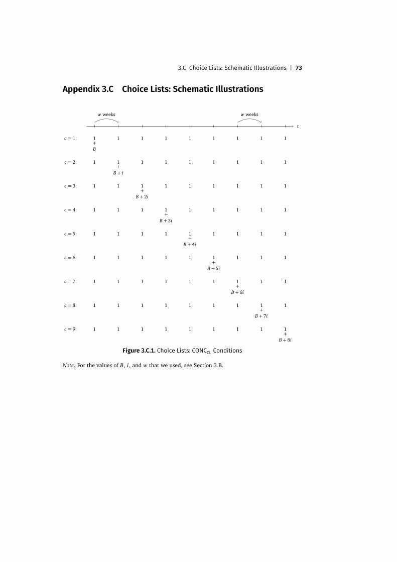
3.C Choice Lists: Schematic Illustrations | 73
Appendix 3.C Choice Lists: Schematic Illustrations
w weeks w weeks
t
c = 1: 1+B
1 1 1 1 1 1 1 1
c = 2: 1+
B + i
1 1 1 1 1 1 1 1
c = 3:+
B + 2i
1 1 1 1 1 1 1 1 1
c = 4:+
B + 3i
1 1 1 1 1 1 1 1 1
c = 5:+
B + 4i
1 1 1 1 1 1 1 1 1
c = 6:+
B + 5i
1 1 1 1 1 1 1 1 1
c = 7:+
B + 6i
1 1 1 1 1 1 1 1 1
c = 8:+
B + 7i
1 1 1 1 1 1 1 1 1
c = 9:+
B + 8i
1 1 1 1 1 1 1 1 1
Figure 3.C.1. Choice Lists: CONCCL Conditions
Note: For the values of B, i, and w that we used, see Section 3.B.
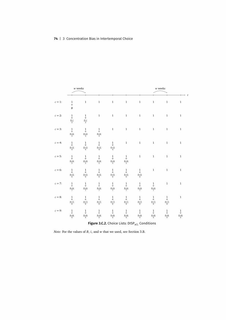
74 | 3 Concentration Bias in Intertemporal Choice
t
w weeks w weeks
c = 1: 1+B
1 1 1 1 1 1 1 1
c = 2: 1+
B+i2
+B+i
2
1 1 1 1 1 1 1 1
c = 3:+
B+2i3
+B+2i
3
+B+2i
3
1 1 1 1 1 1 1 1 1
c = 4:+
B+3i4
+B+3i
4
+B+3i
4
+B+3i
4
1 1 1 1 1 1 1 1 1
c = 5:+
B+4i5
+B+4i
5
+B+4i
5
+B+4i
5
+B+4i
5
1 1 1 1 1 1 1 1 1
c = 6:+
B+5i6
+B+5i
6
+B+5i
6
+B+5i
6
+B+5i
6
+B+5i
6
1 1 1 1 1 1 1 1 1
c = 7:+
B+6i7
+B+6i
7
+B+6i
7
+B+6i
7
+B+6i
7
+B+6i
7
+B+6i
7
1 1 1 1 1 1 1 1 1
c = 8:+
B+7i8
+B+7i
8
+B+7i
8
+B+7i
8
+B+7i
8
+B+7i
8
+B+7i
8
+B+7i
8
1 1 1 1 1 1 1 1 1
c = 9:+
B+8i9
+B+8i
9
+B+8i
9
+B+8i
9
+B+8i
9
+B+8i
9
+B+8i
9
+B+8i
9
+B+8i
9
1 1 1 1 1 1 1 1 1
Figure 3.C.2. Choice Lists: DISPaCL Conditions
Note: For the values of B, i, and w that we used, see Section 3.B.
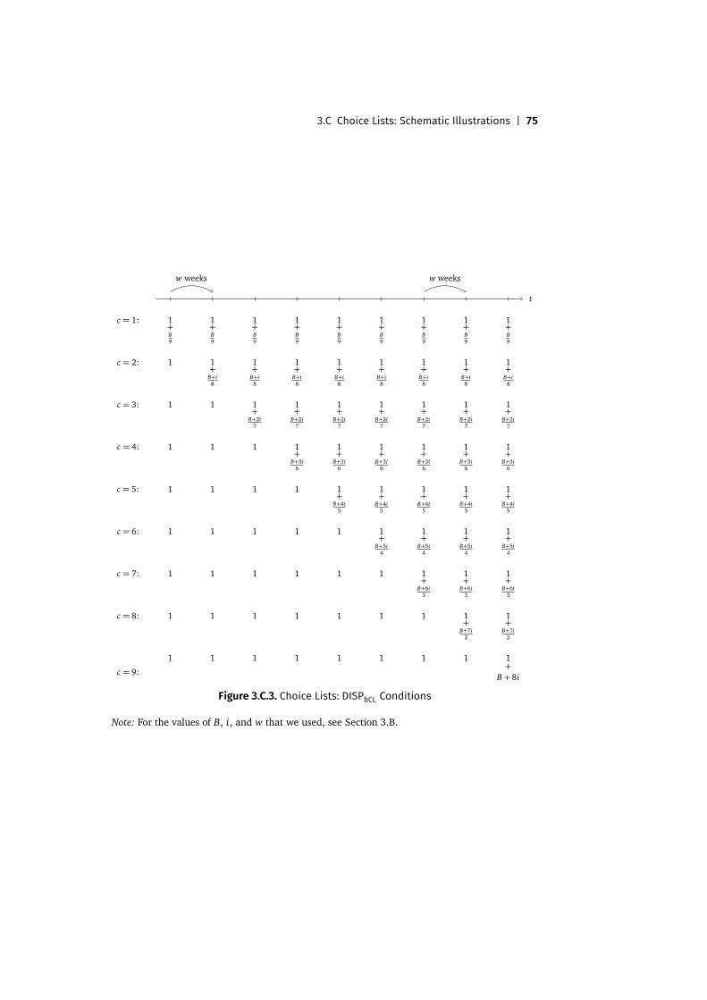
3.C Choice Lists: Schematic Illustrations | 75
t
w weeks w weeks
c = 1: 1+B9
1+B9
1+B9
1+B9
1+B9
1+B9
1+B9
1+B9
1+B9
c = 2: 1 1+
B+i8
1+
B+i8
1+
B+i8
1+
B+i8
1+
B+i8
1+
B+i8
1+
B+i8
1+
B+i8
c = 3: 1 1 1+
B+2i7
1+
B+2i7
1+
B+2i7
1+
B+2i7
1+
B+2i7
1+
B+2i7
1+
B+2i7
c = 4: 1 1 1 1+
B+3i6
1+
B+3i6
1+
B+3i6
1+
B+3i6
1+
B+3i6
1+
B+3i6
c = 5: 1 1 1 1 1+
B+4i5
1+
B+4i5
1+
B+4i5
1+
B+4i5
1+
B+4i5
c = 6: 1 1 1 1 1 1+
B+5i4
1+
B+5i4
1+
B+5i4
1+
B+5i4
c = 7: 1 1 1 1 1 1 1+
B+6i3
1+
B+6i3
1+
B+6i3
c = 8: 1 1 1 1 1 1 1 1+
B+7i2
1+
B+7i2
c = 9:+
B + 8i
1 1 1 1 1 1 1 1 1
Figure 3.C.3. Choice Lists: DISPbCL Conditions
Note: For the values of B, i, and w that we used, see Section 3.B.

76 | 3 Concentration Bias in Intertemporal Choice
Appendix 3.D Choice Lists: Comparison between CONCb andDISPb
We look at people whose behavior can be described with exponential discount-ing. We intend to show that those who are patient in the long decreasingly dis-persed treatment must be patient in the short concentrated treatment, too. Forinstance, if someone chooses slider position n in the first treatment, he shouldchoose at least n in the latter one. We use linear utility and show (numerically)that there is a bigger interval of possible δs such that option n is chosen overoption n− 1 for the short concentrated treatment than the long decreasinglydispersed treatment.
Concentrated (short)
Choosing slider position n over n− 1 amounts to:
δn(b + r) > δn−1 b ⇔ δ(b + r) > b ⇔ δ >b
b + r=: δconc ,
where b is the received payoff in period n− 1 and r the interest payment accru-ing between the two payment dates.
Decreasingly dispersed (long)
Choosing slider position n over n− 1 amounts to (n≥ 2):
9−1∑
i=n−1
(δ2)i b + r9 − (n − 1)
>
9−1∑
i=n−2
(δ2)i b9 − ((n − 1) − 1)
⇔b + r
b9 − ((n − 1) − 1)
9 − (n − 1)>
∑8i=n−2(δ
2)i
∑8i=n−1(δ
2)i
=((δ2)n−2 − (δ2)9) /(1 − δ2)((δ2)n−1 − (δ2)9) /(1 − δ2)
⇔b + r
b11 − n10 − n
>((δ2)n−2 − (δ2)9)((δ2)n−1 − (δ2)9)
.
4
How Stable Is Trust?The Case of Personal Experienceof Unfair and Fair Treatment?
Joint with Florian Zimmermann
4.1 Introduction
Trust is a pervasive feature of human relationships. In economics, trust consti-tutes a social lubricant for any kind of transactions when contracts are incom-plete or too costly to be enforced (Arrow, 1974). In particular, trust allows therealization of (efficiency) gains from trade and cooperation. However, it requiresindividuals to make themselves and their resources vulnerable to exploitation byothers.
Ample evidence suggests that trust fosters aggregate social and economicoutcomes (see, e.g., Putnam, 1995; La Porta et al., 1997; Knack and Keefer,1997; Guiso et al., 2004). Understanding how individuals’ willingness to trustcan be encouraged hence poses important challenges for the social sciencesand has potentially far-reaching implications for policy and workplace design.Whether individuals trust others is largely determined by an interplay of theinstitutional setting—capturing the incentives and constraints that individualsface—and individual primitives—i.e., beliefs and preferences.1
Traditionally, economic research has focused primarily on institutional fac-tors. In the case of improving trust, institutions do so by facilitating reputational
? We would like to thank Holger Gerhardt and Simone Quercia for helpful comments.1 This is not to say that institutions and individual primitives are unrelated entities (see, e.g.,
Greif, 1994).
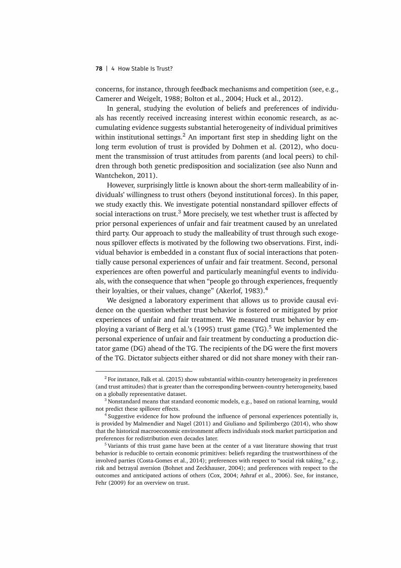
78 | 4 How Stable Is Trust?
concerns, for instance, through feedback mechanisms and competition (see, e.g.,Camerer and Weigelt, 1988; Bolton et al., 2004; Huck et al., 2012).
In general, studying the evolution of beliefs and preferences of individu-als has recently received increasing interest within economic research, as ac-cumulating evidence suggests substantial heterogeneity of individual primitiveswithin institutional settings.2 An important first step in shedding light on thelong term evolution of trust is provided by Dohmen et al. (2012), who docu-ment the transmission of trust attitudes from parents (and local peers) to chil-dren through both genetic predisposition and socialization (see also Nunn andWantchekon, 2011).
However, surprisingly little is known about the short-term malleability of in-dividuals’ willingness to trust others (beyond institutional forces). In this paper,we study exactly this. We investigate potential nonstandard spillover effects ofsocial interactions on trust.3 More precisely, we test whether trust is affected byprior personal experiences of unfair and fair treatment caused by an unrelatedthird party. Our approach to study the malleability of trust through such exoge-nous spillover effects is motivated by the following two observations. First, indi-vidual behavior is embedded in a constant flux of social interactions that poten-tially cause personal experiences of unfair and fair treatment. Second, personalexperiences are often powerful and particularly meaningful events to individu-als, with the consequence that when “people go through experiences, frequentlytheir loyalties, or their values, change” (Akerlof, 1983).4
We designed a laboratory experiment that allows us to provide causal evi-dence on the question whether trust behavior is fostered or mitigated by priorexperiences of unfair and fair treatment. We measured trust behavior by em-ploying a variant of Berg et al.’s (1995) trust game (TG).5 We implemented thepersonal experience of unfair and fair treatment by conducting a production dic-tator game (DG) ahead of the TG. The recipients of the DG were the first moversof the TG. Dictator subjects either shared or did not share money with their ran-
2 For instance, Falk et al. (2015) show substantial within-country heterogeneity in preferences(and trust attitudes) that is greater than the corresponding between-country heterogeneity, basedon a globally representative dataset.
3Nonstandard means that standard economic models, e.g., based on rational learning, wouldnot predict these spillover effects.
4 Suggestive evidence for how profound the influence of personal experiences potentially is,is provided by Malmendier and Nagel (2011) and Giuliano and Spilimbergo (2014), who showthat the historical macroeconomic environment affects individuals stock market participation andpreferences for redistribution even decades later.
5 Variants of this trust game have been at the center of a vast literature showing that trustbehavior is reducible to certain economic primitives: beliefs regarding the trustworthiness of theinvolved parties (Costa-Gomes et al., 2014); preferences with respect to “social risk taking,” e.g.,risk and betrayal aversion (Bohnet and Zeckhauser, 2004); and preferences with respect to theoutcomes and anticipated actions of others (Cox, 2004; Ashraf et al., 2006). See, for instance,Fehr (2009) for an overview on trust.
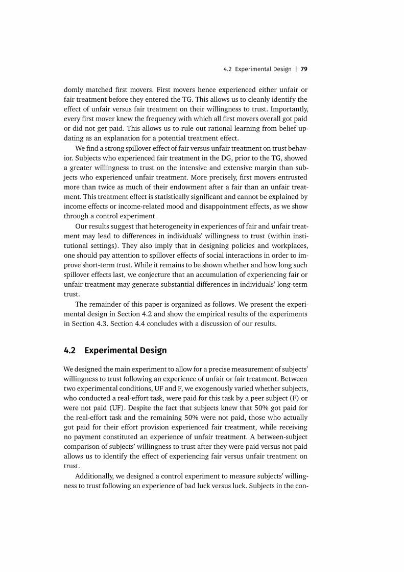
4.2 Experimental Design | 79
domly matched first movers. First movers hence experienced either unfair orfair treatment before they entered the TG. This allows us to cleanly identify theeffect of unfair versus fair treatment on their willingness to trust. Importantly,every first mover knew the frequency with which all first movers overall got paidor did not get paid. This allows us to rule out rational learning from belief up-dating as an explanation for a potential treatment effect.
We find a strong spillover effect of fair versus unfair treatment on trust behav-ior. Subjects who experienced fair treatment in the DG, prior to the TG, showeda greater willingness to trust on the intensive and extensive margin than sub-jects who experienced unfair treatment. More precisely, first movers entrustedmore than twice as much of their endowment after a fair than an unfair treat-ment. This treatment effect is statistically significant and cannot be explained byincome effects or income-related mood and disappointment effects, as we showthrough a control experiment.
Our results suggest that heterogeneity in experiences of fair and unfair treat-ment may lead to differences in individuals’ willingness to trust (within insti-tutional settings). They also imply that in designing policies and workplaces,one should pay attention to spillover effects of social interactions in order to im-prove short-term trust. While it remains to be shown whether and how long suchspillover effects last, we conjecture that an accumulation of experiencing fair orunfair treatment may generate substantial differences in individuals’ long-termtrust.
The remainder of this paper is organized as follows. We present the experi-mental design in Section 4.2 and show the empirical results of the experimentsin Section 4.3. Section 4.4 concludes with a discussion of our results.
4.2 Experimental Design
Wedesigned themain experiment to allow for a precisemeasurement of subjects’willingness to trust following an experience of unfair or fair treatment. Betweentwo experimental conditions, UF and F, we exogenously varied whether subjects,who conducted a real-effort task, were paid for this task by a peer subject (F) orwere not paid (UF). Despite the fact that subjects knew that 50% got paid forthe real-effort task and the remaining 50% were not paid, those who actuallygot paid for their effort provision experienced fair treatment, while receivingno payment constituted an experience of unfair treatment. A between-subjectcomparison of subjects’ willingness to trust after they were paid versus not paidallows us to identify the effect of experiencing fair versus unfair treatment ontrust.
Additionally, we designed a control experiment to measure subjects’ willing-ness to trust following an experience of bad luck versus luck. Subjects in the con-
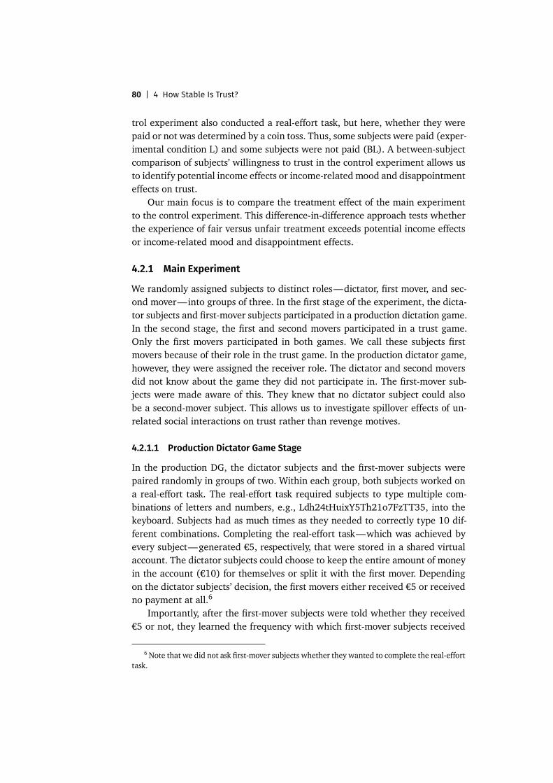
80 | 4 How Stable Is Trust?
trol experiment also conducted a real-effort task, but here, whether they werepaid or not was determined by a coin toss. Thus, some subjects were paid (exper-imental condition L) and some subjects were not paid (BL). A between-subjectcomparison of subjects’ willingness to trust in the control experiment allows usto identify potential income effects or income-related mood and disappointmenteffects on trust.
Our main focus is to compare the treatment effect of the main experimentto the control experiment. This difference-in-difference approach tests whetherthe experience of fair versus unfair treatment exceeds potential income effectsor income-related mood and disappointment effects.
4.2.1 Main Experiment
We randomly assigned subjects to distinct roles—dictator, first mover, and sec-ond mover—into groups of three. In the first stage of the experiment, the dicta-tor subjects and first-mover subjects participated in a production dictation game.In the second stage, the first and second movers participated in a trust game.Only the first movers participated in both games. We call these subjects firstmovers because of their role in the trust game. In the production dictator game,however, they were assigned the receiver role. The dictator and second moversdid not know about the game they did not participate in. The first-mover sub-jects were made aware of this. They knew that no dictator subject could alsobe a second-mover subject. This allows us to investigate spillover effects of un-related social interactions on trust rather than revenge motives.
4.2.1.1 Production Dictator Game Stage
In the production DG, the dictator subjects and the first-mover subjects werepaired randomly in groups of two. Within each group, both subjects worked ona real-effort task. The real-effort task required subjects to type multiple com-binations of letters and numbers, e.g., Ldh24tHuixY5Th21o7FzTT35, into thekeyboard. Subjects had as much times as they needed to correctly type 10 dif-ferent combinations. Completing the real-effort task—which was achieved byevery subject—generated €5, respectively, that were stored in a shared virtualaccount. The dictator subjects could choose to keep the entire amount of moneyin the account (€10) for themselves or split it with the first mover. Dependingon the dictator subjects’ decision, the first movers either received €5 or receivedno payment at all.6
Importantly, after the first-mover subjects were told whether they received€5 or not, they learned the frequency with which first-mover subjects received
6Note that we did not ask first-mover subjects whether they wanted to complete the real-efforttask.
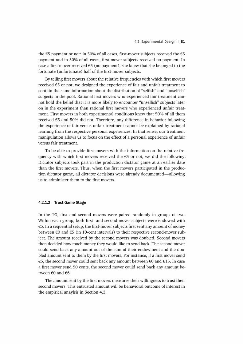
4.2 Experimental Design | 81
the €5 payment or not: in 50% of all cases, first-mover subjects received the €5payment and in 50% of all cases, first-mover subjects received no payment. Incase a first mover received €5 (no payment), she knew that she belonged to thefortunate (unfortunate) half of the first-mover subjects.
By telling first movers about the relative frequencies with which first moversreceived €5 or not, we designed the experience of fair and unfair treatment tocontain the same information about the distribution of “selfish” and “unselfish”subjects in the pool. Rational first movers who experienced fair treatment can-not hold the belief that it is more likely to encounter “unselfish” subjects lateron in the experiment than rational first movers who experienced unfair treat-ment. First movers in both experimental conditions knew that 50% of all themreceived €5 and 50% did not. Therefore, any difference in behavior followingthe experience of fair versus unfair treatment cannot be explained by rationallearning from the respective personal experiences. In that sense, our treatmentmanipulation allows us to focus on the effect of a personal experience of unfairversus fair treatment.
To be able to provide first movers with the information on the relative fre-quency with which first movers received the €5 or not, we did the following.Dictator subjects took part in the production dictator game at an earlier datethan the first movers. Thus, when the first movers participated in the produc-tion dictator game, all dictator decisions were already documented—allowingus to administer them to the first movers.
4.2.1.2 Trust Game Stage
In the TG, first and second movers were paired randomly in groups of two.Within each group, both first- and second-mover subjects were endowed with€5. In a sequential setup, the first-mover subjects first sent any amount of moneybetween €0 and €5 (in 10-cent intervals) to their respective second-mover sub-ject. The amount received by the second movers was doubled. Second moversthen decided how much money they would like to send back. The second movercould send back any amount out of the sum of their endowment and the dou-bled amount sent to them by the first movers. For instance, if a first mover send€5, the second mover could sent back any amount between €0 and €15. In casea first mover send 50 cents, the second mover could send back any amount be-tween €0 and €6.
The amount sent by the first movers measures their willingness to trust theirsecond movers. This entrusted amount will be behavioral outcome of interest inthe empirical anaylsis in Section 4.3.
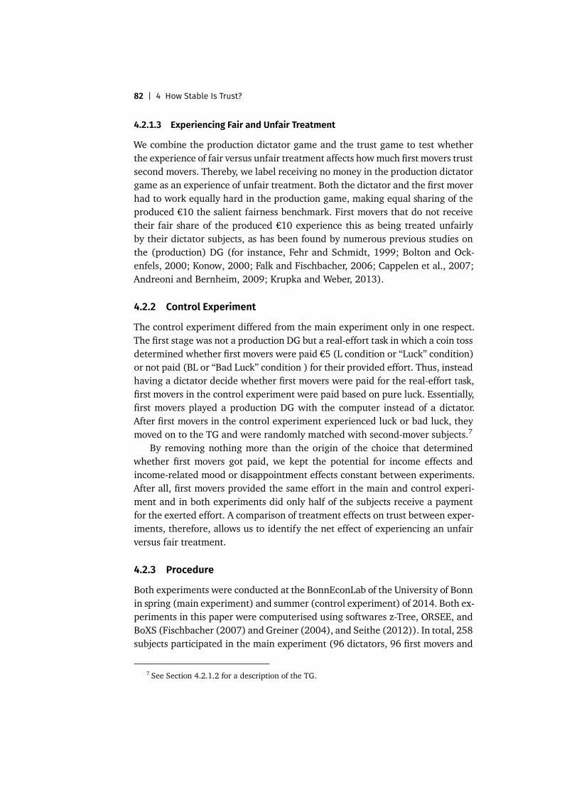
82 | 4 How Stable Is Trust?
4.2.1.3 Experiencing Fair and Unfair Treatment
We combine the production dictator game and the trust game to test whetherthe experience of fair versus unfair treatment affects howmuch first movers trustsecond movers. Thereby, we label receiving no money in the production dictatorgame as an experience of unfair treatment. Both the dictator and the first moverhad to work equally hard in the production game, making equal sharing of theproduced €10 the salient fairness benchmark. First movers that do not receivetheir fair share of the produced €10 experience this as being treated unfairlyby their dictator subjects, as has been found by numerous previous studies onthe (production) DG (for instance, Fehr and Schmidt, 1999; Bolton and Ock-enfels, 2000; Konow, 2000; Falk and Fischbacher, 2006; Cappelen et al., 2007;Andreoni and Bernheim, 2009; Krupka and Weber, 2013).
4.2.2 Control Experiment
The control experiment differed from the main experiment only in one respect.The first stage was not a production DG but a real-effort task in which a coin tossdetermined whether first movers were paid €5 (L condition or “Luck” condition)or not paid (BL or “Bad Luck” condition ) for their provided effort. Thus, insteadhaving a dictator decide whether first movers were paid for the real-effort task,first movers in the control experiment were paid based on pure luck. Essentially,first movers played a production DG with the computer instead of a dictator.After first movers in the control experiment experienced luck or bad luck, theymoved on to the TG and were randomly matched with second-mover subjects.7
By removing nothing more than the origin of the choice that determinedwhether first movers got paid, we kept the potential for income effects andincome-related mood or disappointment effects constant between experiments.After all, first movers provided the same effort in the main and control experi-ment and in both experiments did only half of the subjects receive a paymentfor the exerted effort. A comparison of treatment effects on trust between exper-iments, therefore, allows us to identify the net effect of experiencing an unfairversus fair treatment.
4.2.3 Procedure
Both experiments were conducted at the BonnEconLab of the University of Bonnin spring (main experiment) and summer (control experiment) of 2014. Both ex-periments in this paper were computerised using softwares z-Tree, ORSEE, andBoXS (Fischbacher (2007) and Greiner (2004), and Seithe (2012)). In total, 258subjects participated in the main experiment (96 dictators, 96 first movers and
7 See Section 4.2.1.2 for a description of the TG.
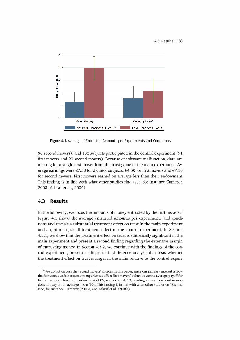
4.3 Results | 83
Figure 4.1. Average of Entrusted Amounts per Experiments and Conditions
96 second movers), and 182 subjects participated in the control experiment (91first movers and 91 second movers). Because of software malfunction, data aremissing for a single first mover from the trust game of the main experiment. Av-erage earnings were €7.50 for dictator subjects, €4.50 for first movers and €7.10for second movers. First movers earned on average less than their endowment.This finding is in line with what other studies find (see, for instance Camerer,2003; Ashraf et al., 2006).
4.3 Results
In the following, we focus the amounts of money entrusted by the first movers.8
Figure 4.1 shows the average entrusted amounts per experiments and condi-tions and reveals a substantial treatment effect on trust in the main experimentand an, at most, small treatment effect in the control experiment. In Section4.3.1, we show that the treatment effect on trust is statistically significant in themain experiment and present a second finding regarding the extensive marginof entrusting money. In Secton 4.3.2, we continue with the findings of the con-trol experiment, present a difference-in-difference analysis that tests whetherthe treatment effect on trust is larger in the main relative to the control experi-
8We do not discuss the second movers’ choices in this paper, since our primary interest is howthe fair versus unfair treatment experiences affect first movers’ behavior. As the average payoff forfirst movers is below their endowment of €5, see Section 4.2.3, sending money to second moversdoes not pay off on average in our TGs. This finding is in line with what other studies on TGs find(see, for instance, Camerer (2003), and Ashraf et al. (2006)).
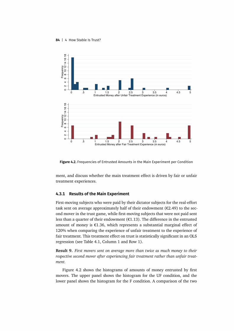
84 | 4 How Stable Is Trust?
02
46
810
1214
1618
Freq
uenc
y
0 .5 1 1.5 2 2.5 3 3.5 4 4.5 5Entrusted Money after Unfair Treatment Experience (in euros)
02
46
810
1214
1618
Freq
uenc
y
0 .5 1 1.5 2 2.5 3 3.5 4 4.5 5Entrusted Money after Fair Treatment Experience (in euros)
Figure 4.2. Frequencies of Entrusted Amounts in the Main Experiment per Condition
ment, and discuss whether the main treatment effect is driven by fair or unfairtreatment experiences.
4.3.1 Results of the Main Experiment
First-moving subjects who were paid by their dictator subjects for the real-efforttask sent on average approximately half of their endowment (€2.49) to the sec-ond mover in the trust game, while first-moving subjects that were not paid sentless than a quarter of their endowment (€1.13). The difference in the entrustedamount of money is €1.36, which represents a substantial marginal effect of120% when comparing the experience of unfair treatment to the experience offair treatment. This treatment effect on trust is statistically significant in an OLSregression (see Table 4.1, Column 1 and Row 1).
Result 9. First movers sent on average more than twice as much money to theirrespective second mover after experiencing fair treatment rather than unfair treat-ment.
Figure 4.2 shows the histograms of amounts of money entrusted by firstmovers. The upper panel shows the histogram for the UF condition, and thelower panel shows the histogram for the F condition. A comparison of the two
4.3 Results | 85
Table 4.1. Comparing Treatment Effects on Trust between Main and Control Experiment
OLS: Logit:Entrusted Amount Entrusted Amount > 0
(1) (2)
1 if Not Paid −1.36*** −1.14**(0.30) (0.51)
1 if Control Experiment −0.92*** −0.95*(0.34) (0.52)
1 if Not Paid and Control 1.07** 1.17*(0.46) (0.68)
Constant 2.49*** 1.74***(0.27) (0.41)
Observations 186 186Adj./Pseudo R2 0.09 0.03
Notes: In Column 1, we regress the entrusted amount on a condition dummy (= 1 for UF or BL),an experiment dummy (= 1 for the control experiment) and an interaction variable between thetwo dummies. In Column 2, a logistic regression on a different dependent variable—whether theentrusted amount was larger than €0 (= 1) or not (= 0)—repeats the analyses of Column 1. Westate (robust) standard errors in parentheses. Significant at the 1 (5) [10] percent level: *** (**)[*].
histograms provides further support for Result 9. While only 7 first movers didnot send any money and only 9 subjects sent less than €1 to their respectivesecond movers after experiencing fair treatment, 17 first movers did not sendany money and 26 subjects sent less than €1 after experiencing unfair treatment.The likelihood that first movers sent a positive amount of money is larger in theF condition rather than the UF condition. This treatment effect is statisticallysignificant in a logistic regression (see Table 4.1, Column 2 and Row 1).
Result 10. The likelihood of first movers sending a positive amount of money totheir respective second mover is significantly larger after experiencing fair ratherthan unfair treatment.
4.3.2 Main versus Control Experiment
We now turn to the control experiment. Figure 4.3 reveals that first movers sentfairly similar amounts of money to their respective second movers in both L andBL conditions. On average, unlucky first movers (condition BL) sent €0.29 lessthan lucky first movers (condition L). This treatment effect is not statisticallysignificant in an OLS regression (p < 0.397) and significantly smaller relative tothe treatment effect of the main experiment (see Table 4.1, Column 1 and Row
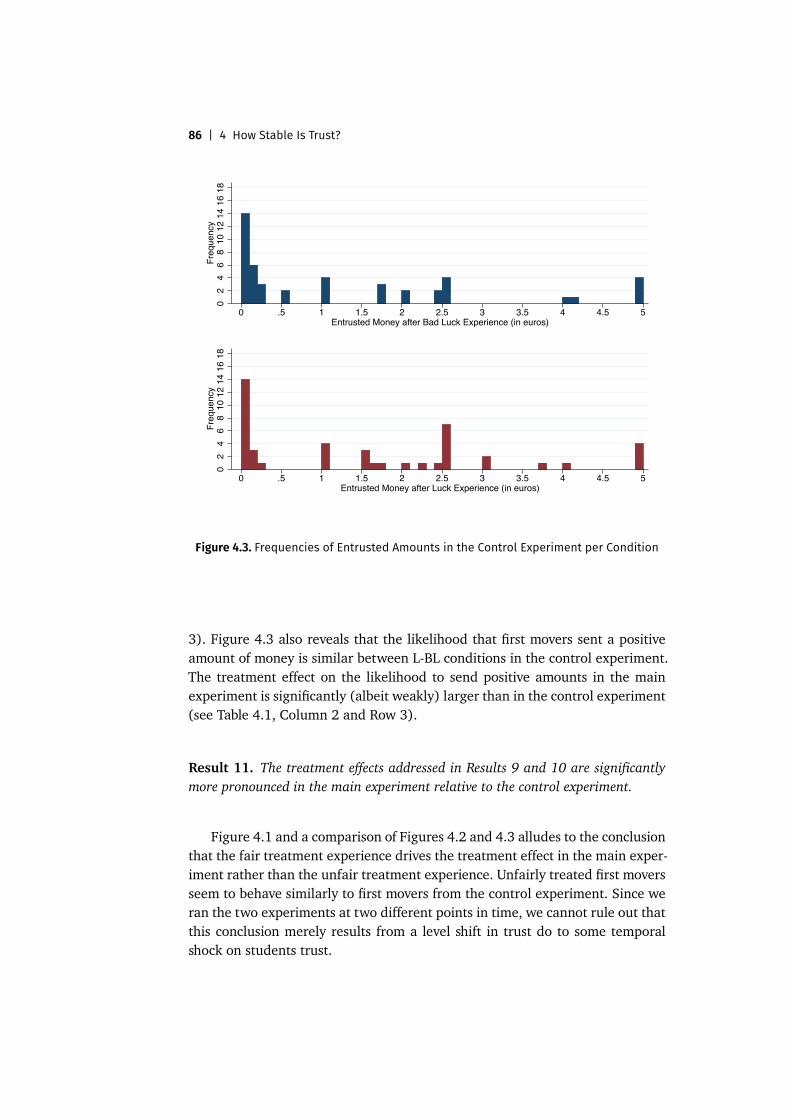
86 | 4 How Stable Is Trust?
02
46
810
1214
1618
Freq
uenc
y
0 .5 1 1.5 2 2.5 3 3.5 4 4.5 5Entrusted Money after Bad Luck Experience (in euros)
02
46
810
1214
1618
Freq
uenc
y
0 .5 1 1.5 2 2.5 3 3.5 4 4.5 5Entrusted Money after Luck Experience (in euros)
Figure 4.3. Frequencies of Entrusted Amounts in the Control Experiment per Condition
3). Figure 4.3 also reveals that the likelihood that first movers sent a positiveamount of money is similar between L-BL conditions in the control experiment.The treatment effect on the likelihood to send positive amounts in the mainexperiment is significantly (albeit weakly) larger than in the control experiment(see Table 4.1, Column 2 and Row 3).
Result 11. The treatment effects addressed in Results 9 and 10 are significantlymore pronounced in the main experiment relative to the control experiment.
Figure 4.1 and a comparison of Figures 4.2 and 4.3 alludes to the conclusionthat the fair treatment experience drives the treatment effect in the main exper-iment rather than the unfair treatment experience. Unfairly treated first moversseem to behave similarly to first movers from the control experiment. Since weran the two experiments at two different points in time, we cannot rule out thatthis conclusion merely results from a level shift in trust do to some temporalshock on students trust.
4.4 Discussion | 87
4.4 Discussion
Our results show a substantial effect of personally experiencing unfair versusfair treatment on subjects’ willingness to trust others. Result 11 reveals thatthis treatment effect on trust cannot be explained by income effects or income-related mood and disappointment effects. Additionally, we can rule out rationallearning explanations, as we told first movers in the main experiment about therelative frequencies of dictator behavior before they entered the TG (see Section4.2.1.1).
Based on these findings, policy makers and workplace designers who are in-terested in promoting trust should keep spillover effects from unrelated personalexperiences in mind. By encouraging fairness between individuals, trust may befostered as a welcomed side effect and virtuous circles may be initiated.9
Personal experiences of fair versus unfair treatment may affect individuals’trust because of the following reasons. First, individuals overweight personallyexperienced states of the world. In particular, fairly treated first movers mayoverweight—relative to the rational benchmark—the likelihood of being fairlytreated again in the near future. Second, indirect reciprocity urges individualsto “respond in kind” to others based on previous interactions with someone else.In the experiment, fairly treated first movers may want to respond indirectly inkind to dictator behavior by offering the second mover efficiency gains from theTG.
Our design does not allow us to differentiate between the two accounts interms of which one is driving our results. This remains to be an interesting ques-tion for future research.
References
Akerlof, George A. (1983): “Loyalty Filters.” American Economic Review, 71 (1), 54–63. [78]Andreoni, James and B. Douglas Bernheim (2009): “Social Image and the 50-50 Norm:
A Theoretical and Experimental Analysis of Audience Effects.” Econometrica, 77 (5),1607–1636. [82]
Arrow, Kenneth (1974): The Limits of Organization. New York: W. W. Norton & Comp. Inc.,pp. 1–86. [77]
Ashraf, Nava, Iris Bohnet, and Nikita Piankov (2006): “Decomposing trust and trustworthi-ness.” Experimental Economics, 9 (3), 193–208. [78, 83]
Berg, Joyce, John Dickhaut, and Kevin McCabe (1995): Trust, Reciprocity, and Social History.[78]
Bohnet, Iris and Richard J. Zeckhauser (2004): “Trust, Risk and Betrayal.” Journal of Eco-nomic Behavior & Organization, 55 (4), 467–484. [78]
9However, one should be cautionary, as trust may be promoted in situations that lead to ex-ploitation. In our TG, for instance, first movers who experienced fair treatment earned 54 Centson average less than first movers who experienced unfair treatment.
88 | 4 How Stable Is Trust?
Bolton, Gary E., Elena Katok, and Axel Ockenfels (2004): “How Effective Are Electronic Rep-utation Mechanisms? An Experimental Investigation.” Management Science, 50 (11),1587–1602. [78]
Bolton, Gary E. and Axel Ockenfels (2000): “ERC: A Theory of Equity, Reciprocity, and Com-petition.” American Economic Review, 90 (1), 166–193. [82]
Camerer, Colin F. (2003): “Strategizing in the Brain.” Science, 2144 (June), 1673–1676. [83]Camerer, Colin F. andKeithWeigelt (1988): “Experimental Tests of a Sequential Equilibrium
Reputation Model.” Econometrica, 56 (1), 1–36. [78]Cappelen, AlexanderW., Astri Drange Hole, Erik Ø. Sørensen, and Bertil Tungodden (2007):
“The Pluralism of Fairness Ideals: An Experimental Approach.” American Economic Re-view, 97 (3), 818–827. [82]
Costa-Gomes, Miguel A., Steffen Huck, and Georg Weizsäcker (2014): “Beliefs and Actionsin the Trust Game: Creating Instrumental Variables to Estimate the Causal Effect.”Games and Economic Behavior, 88, 298–309. [78]
Cox, James C. (2004): “How to Identify Trust and Reciprocity.” Games and Economic Behav-ior, 46 (2), 260–281. [78]
Dohmen, Thomas, Armin Falk, David Huffman, and Uwe Sunde (2012): “The Intergenera-tional Transmission of Risk and Trust Attitudes.” Review of Economic Studies, 79 (2),645–677. [78]
Falk, Armin, Anke Becker, Thomas Dohmen, Benjamin Enke, David Huffman, and UweSunde (2015): “The Nature and Predictive Power of Preferences: Global Evidence.”Working Paper, 1–76. [78]
Falk, Armin and Urs Fischbacher (2006): “A Theory of Reciprocity.” Games and EconomicBehavior, 54 (2), 293–315. [82]
Fehr, Ernst (2009): “On the Economics and Biology of Trust.” Journal of the European Eco-nomic Association, 7 (2-3), 235–266. [78]
Fehr, Ernst and Klaus M. Schmidt (1999): “A Theory Of Fairness, Competition, and Cooper-ation.” Quarterly Journal of Economics, 114 (3), 817–868. [82]
Fischbacher, Urs (2007): “z-Tree: Zurich Toolbox for Ready-Made Economic Experiments.”Experimental Economics, 10 (2), 171–178. [82]
Giuliano, Paola and Antonio Spilimbergo (2014): “Growing up in a Recession.” Review ofEconomic Studies, 81 (2), 787–817. [78]
Greif, Avner (1994): “Cultural Beliefs and the Organization of Society: A Historical and Theo-retical Reflection on Collectivist and Individualist Societies.” Journal of Political Econ-omy, 102 (5), 912. [77]
Greiner, Ben (2004): “An Online Recruitment System For Economic Experiments.”Forschung und Wissenschaftliches Rechnen, 63, 79–93. [82]
Guiso, L, P Sapienza, and L Zingales (2004): “The role of social capital in financial devel-opment.” American Economic Review, 94 (3), 526–556. [77]
Huck, Steffen, Gabriele K. Lünser, and Jean Robert Tyran (2012): “Competition fosterstrust.” Games and Economic Behavior, 76 (1), 195–209. [78]
Knack, Stephen and Philip Keefer (1997): “Does Social Capital Have an Economic Payoff?”Quarterly Journal of Economics, 112 (4), 1251–1288. [77]
Konow, James (2000): “Fair Shares: Accountability and Cognitive Dissonance in AllocationDecisions.” American Economic Review, 90 (4), 1072–1091. [82]
4.A Instructions | 89
Krupka, Erin L. and Roberto A. Weber (2013): “Identifying Social Norms Using CoordinationGames: Why Does Dictator Game Sharing Vary?” Journal of the European EconomicAssociation, 11 (3), 495–524. [82]
La Porta, Rafael, Florencio Lopez-de-Silanes, Andrei Shleifer, and RobertW. Vishny (1997):“Trust in Large Organizations.” American Economic Review, Papers and Proceedings,87 (2), 333–338. [77]
Malmendier, Ulrike and Stefan Nagel (2011): “Depression Babies: Do Macroeconomic Ex-periences Affect Risk Taking?” Quarterly Journal of Economics, 126 (1), 373–416. [78]
Nunn, Nathan and Leonard Wantchekon (2011): “The Slave Trade and the Origins of Mis-trust in Africa.” American Economic Review, 101 (7), 3221–3252. [78]
Putnam, Robert D (1995): “Bowling Alone: American’s Declining Social Capital.” Journal ofDemocracy, 6 (1), 65–78. [77]
Seithe, Mirko (2012): “Introducing the Bonn Experiment System (BoXS).” Bonn Econ Dis-cussion Paper. [82]
Appendix 4.A Instructions
Main experiment, first mover, F [UF] condition
Production Dictator Game
This experiment consists of two parts. Your payments for part 1 and part 2 areindependent of each other. You get paid in cash at the end of the experiment.
You participate with a different subject in each part of the experiment.
A participant is randomly assigned from a group of participants to partici-pate with you in part 1. Your participant only participated in part 1 and has noknowledge regarding part 2. Your participant took part in part 1 at an earlierdate and is not present in the laboratory today.
A participant from another group of participants is randomly assigned toparticipate with you in part 2. Your participant in part 2 participated only inpart 2 and has no knowledge regarding part 1. Your participant in part 2 tookpart in part 2 at an earlier date and is not present in the laboratory today.
Please note that: First, the groups from which your first and your secondparticipant are randomly chosen from are not identical. No member from onegroup is also amember in the other group. Second, youwill never know anythingabout your two participants and your identify is not revealed to anyone in thisexperiment.
[next screen]
Part 1

90 | 4 How Stable Is Trust?
Your task and the task of your first participant is to type combinations ofnumbers and letters into the keyboard.
For instance: Ldh24tHuixY5Th21o7FzTT35
You will see combinations of numbers and letters on your screen. Typethese numbers and letters one by one into the entry field below and do thiscase-sensitive. After you have typed a combination into the keyboard, press the“continue”-button. After you have typed a combination into the keyboard andpressed the button, a new combination appears.
[next screen]
For you:
You receive 25 cents for any correctly typed combination. You need to ac-cumulate €2.50 and you have as much time as you need to do so. You cannotaccumulate more or less than €2.50. The experiment will not continue unlessyou have accumulated €2.50.
For your participant:
Your participant also accumulated €2.50, not more and not less.
Shared account:
Both amounts of money are stored in a shared account. The conductors of theexperiment double this amount such that €10 are stored in your joint account.
[next screen]
Your payment:
As explained above, €10 are on your joint account.
Your participant will decide how the €10 are shared between the two ofyou. Your participant can allocate the money fairly such that both of you receive€5. Your participant can also allocate the money unfairly such that both yourparticipant receives the entire €10 receive.
As explained above, your participant already took part in this experiment atan earlier date. Thus, your participant has already decided how to allocate the€10. Your participate has already decided whether you receive €5 or whetheryou receive no payment at all.
Comprehension question: Which amount of money cannot be earned by youin part 1? €0 or €2.50 or €5.00.
4.A Instructions | 91
[next screen]
Before you will be made aware that you do or do not receive €5, we wouldlike you to accumulate €2.50 in the typing-task.
[next screen]
typing-task[next screen]
Thank you for accumulating €2.50. Your participant has also accumulated€2.50. Additionally, the conductors of the experiment added another €5 to yourjoint account such that €10 are on your joint account.
You will be informed how much money your participant shared with you onthe next screen.
[next screen]
Your participant has allocated the €10 such that you receive €5 [0]. There-fore, your payoff for part 1 is €5 [0].
Please notice that your participate was randomly assigned to you from agroup of potential participants. In this group of potential participants 48 out of96 shared the €10 evenly and 48 out of 96 kept the entire €10 for themselves.
Trust Game
[next screen]
In part 2 you and your participant receive two different roles: You are thesender. Your second participant is the re-sender. The both of you receive an en-dowment of €5. Part 2 has two stages.
Stage 1:
In stage 1 you can send an amount of money to the re-sender. You can sendany amount of money between €0 and €5 in steps of 10 cents. You can send €0,10 cents, 20 cents, 30 cents, . . . , 90 cents, €1, . . . , €4.80, €4.90, €5. The amountof money that you send will be doubled by the conductors of the experiment.For instance, if you send €2.40, then the re-sender will receive €4.80, and if yousend €0, your re-sender receives €0.
Stage 2:
92 | 4 How Stable Is Trust?
In stage 2 the re-sender is asked to send back an amount of money to you.This amount is doubled. The re-sender chooses an amount between €0 and thesum of his endowment and the doubled amount that you send in the first stage.
Payments:
You will receive: 5 − Amount that you send to the re-sender + Amount thatthe re-sender sends back to you.The re-sender receives: 5+ 2×Amount that you send to the re-sender−Amountthat the re-sender sends back to you.
Example:
Consider the case that you send €2.40, then the re-sender received €4.80.The re-sender can send an amount of money between €0 and €9.80 back to you.For instance, the re-sender could send €3.60 back to you such that the overallamounts is shared fairly between the two of you which means that you bothreceive €6.20.
However, the re-sender could also behave unfairly and not send any amountof money back to you. In this case you would receive 5 − 2.40 = €2.60 and there-sender would receive €9.80.
Please notice that if you do not send any money to the re-sender, your pay-ment for part 2 of the experiment will be €5.
[next screen]
Which amount of money do you want to send to the re-sender?
Control experiment, first mover, L [BL] condition
Production Lottery
This experiment consists of two parts. Your payments for part 1 and part 2 areindependent of each other. You get paid in cash at the end of the experiment.
You participate with a different subject in part 2 of the experiment.
A participant from another group of participants is randomly assigned toparticipate with you in part 2. Your participant in part 2 participated only inpart 2 and has no knowledge regarding part 1. Your participant in part 2 tookpart in part 2 at an earlier date and is not present in the laboratory today.
Please note that: You will never know anything about your participant andyour identify is not revealed to anyone in this experiment.

4.A Instructions | 93
[next screen]
Part 1
Your task is to type combinations of numbers and letters into the keyboard.
For instance: Ldh24tHuixY5Th21o7FzTT35
You will see combinations of numbers and letters on your screen. Typethese numbers and letters one by one into the entry field below and do thiscase-sensitive. After you have typed a combination into the keyboard, press the“continue”-button. After you have typed a combination into the keyboard andpressed the button, a new combination appears.
[next screen]
For you:
You receive 25 cents for any correctly typed combination. You need to ac-cumulate €2.50 and you have as much time as you need to do so. You cannotaccumulate more or less than €2.50. The experiment will not continue unlessyou have accumulated €2.50.
Your account:
Yourmoney is stored in an account. The conductors of the experiment doublethis amount such that €5 are stored in the account.
[next screen]
Your payment:
As explained above, €5 are on the account.
Whether you will receive the €5 will be determined randomly. You couldreceive the entire €5 or you could receive no payment at all.
Comprehension question: Which amount of money cannot be earned by youin part 1? €0 or €2.50 or €5.00.
[next screen]
Before you will be made aware that you do or do not receive €5, we wouldlike you to accumulate €2.50 in the typing-task.
[next screen]
typing-task

94 | 4 How Stable Is Trust?
[next screen]
Thank you for accumulating €2.50. The conductors of the experiment addedanother €2.50 to your account such that €5 are on your account.
You will be informed how whether you were randomly selected to receivethe €5 or not on the next screen.
[next screen]
The computer randomly chose that you receive €5 [0] for part 1. Therefore,your payoff for part 1 is €5 [0].
Please notice that whether you earned €5 or not was randomly determined.You can think of it as if a ball was was drawn from an urn. In the urn were 96balls. 48 balls were red and 48 were blue. If a red ball would have been drawn,then you had received €5. If a blue ball would have been draw, then you hadreceived €0. In your case, a red [blue] ball was drawn randomly.
Trust Game
Like in Section 4.A