Eric Blayo, Laurent Debreu To cite this version - … · 6 ERIC BLAYO AND LAURENT DEBREU 2. A classiﬁcation of nesting problems 2.1 General framework We are interested in representing

HAL Id: inria-00187576https://hal.inria.fr/inria-00187576

Submitted on 14 Nov 2007

HAL is a multi-disciplinary open accessarchive for the deposit and dissemination of sci-entific research documents, whether they are pub-lished or not. The documents may come fromteaching and research institutions in France orabroad, or from public or private research centers.

L’archive ouverte pluridisciplinaire HAL, estdestinée au dépôt et à la diffusion de documentsscientifiques de niveau recherche, publiés ou non,émanant des établissements d’enseignement et derecherche français ou étrangers, des laboratoirespublics ou privés.

Nesting ocean modelsEric Blayo, Laurent Debreu

To cite this version:Eric Blayo, Laurent Debreu. Nesting ocean models. E. Chassignet and J. Verron. An Integrated Viewof Oceanography: Ocean Weather Forecasting in the 21st Century, Kluwer, 2006. <inria-00187576>

https://hal.inria.fr/inria-00187576

https://hal.archives-ouvertes.fr

Chapter 6

NESTING OCEAN MODELS

Eric Blayo and Laurent DebreuLMC-IMAG and INRIA Rhone-Alpes, Grenoble, France

Abstract This note is focused on the problem of providing boundary conditionsfor regional ocean models. It is shown that usual methods generally donot address the correct problem, but more or less approaching ones. Atentative classification of these methods is proposed. Then their theo-retical foundations are discussed, and recommendations are given.

Keywords: Open boundary conditions, regional models, nesting.

1. Introduction

The use of high resolution regional ocean models has become wide-spread in recent years, in particular due to the development of oper-ational oceanography and coastal management systems. An importantpoint, that has a strong influence on the quality of the results, is the waythat a local model is forced at its open boundaries. Several methods,whose precise contents, theoretical justification, and practical perfor-mances are often somewhat difficult to compare precisely, are presentlyused in actual applications. In this context, the first aim of this note isto provide a tentative classification of these methods (section 1). Thenwe will discuss the one-way (section 2) and two-way (section 3) inter-actions, focusing on the theoretical foundations and practical use of thedifferent approaches. Some final remarks on the available software toolsand on the problem of data assimilation within nested models are givenin sections 4 and 5.

6 ERIC BLAYO AND LAURENT DEBREU

2. A classification of nesting problems

2.1 General framework

We are interested in representing as accurately as possible the oceanin a local domain Ωloc. The circulation is supposed to be described ona time period [0, T ] by a model which can be written symbolically

Lloculoc = floc inΩloc × [0, T ] (1)

with convenient initial conditions at t = 0. Lloc is a partial differentialoperator, uloc is the state variable, and floc the model forcing. Theconditions at the solid boundaries will never be mentioned in this note,since they do not interfere with our subject.

Since Ωloc is not closed, a portion of its boundary does not correspondto a solid wall, and has no physical reality. This artificial interface, alsocalled open boundary (OB), is denoted Γ. The local solution uloc isthus in interaction with the external ocean through Γ, and the difficultyconsists in adequately representing this interaction in order to get a goodapproximation of uloc in Ωloc × [0, T ].

We also assume that we have at our disposal a (probably less accurate)representation of the external ocean, either under the form of some datauext or of an external model

Lextuext = fext in Ωext × [0, T ] (2)

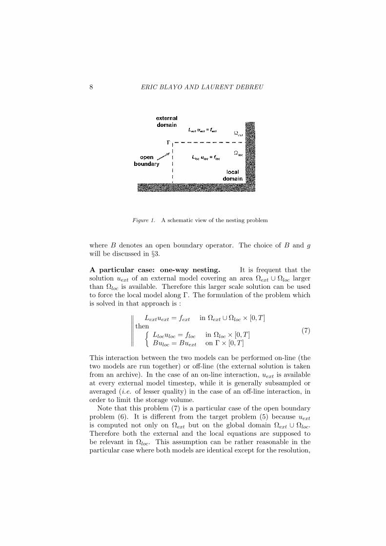
where Ωext is an external oceanic domain. Note that, in our notations,Ωloc and Ωext do not overlap (Figure 1).

The best way to solve the local problem is then probably to use aninverse approach (e.g. Bennett, 2002), i.e. for example

Find uloc that minimizes ‖Lloculoc−floc‖2Ωloc×[0,T ]+ε ‖uloc−uext‖2

Γ×[0,T ]

(3)where the norms are defined conveniently and take into account somestatistical knowledge on the errors on uext and on the model (1), andwhere ε is a weighting factor. One can also consider that the model isperfect, and minimize only ‖uloc−uext‖2

Γ×[0,T ], i.e. control the boundary

values, under the constraint (1) (e.g. Taillandier et al., 2004).However solving such an inverse problem is quite difficult and expen-

sive. That is why ocean modellers usually use direct approaches. Thegoal is then to find uloc satisfying (1) that connects adequately to uext

through Γ. The mathematical formulation of this problem is generallynot expressed clearly in actual applications. Since Γ has no physical real-ity, the connection between uext and uloc should be as smooth as possible,

NESTING OCEAN MODELS 7

i.e. generally continuous and differentiable. Therefore a correct directformulation of the problem can be the following :

∥

∥

∥

∥

∥

∥

∥

∥

∥

∥

Find uloc that satisfies

Lloculoc = floc in Ωloc × [0, T ]

uloc = uext and∂uloc

∂n=

∂uext

∂non Γ × [0, T ]

under the constraint Lextuext = fext in Ωext × [0, T ]

(4)

or equivalently :∥

∥

∥

∥

∥

∥

∥

∥

∥

∥

Find uloc and uext that satisfy

Lloculoc = floc in Ωloc × [0, T ] and Lextuext = fext

in Ωext × [0, T ]

with uloc = uext and∂uloc

∂n=

∂uext

∂non Γ × [0, T ]

(5)

where n denotes the normal direction. However, in actual applications,the external model is not always available for online interaction. More-over it is defined generally on Ωext ∪Ωloc (i.e. it fully overlaps the localdomain), and it would be quite expensive to modify it in order to avoidthis overlapping by implementing an open boundary on Γ. Thereforemost applications generally do not address thecorrect problem (5) itself,but rather more or less approaching problems.

Remark : the operators Lext and Lloc generally differ, both in theircontinuous form (e.g. subgrid scale paramaterizations) and in their dis-cretized form (the local numerical model often has a higher resolutionthan the external model). Moreover the forcings fext and floc, and thediscretized bathymetries defining Ωext and Ωloc can be rather different.In that case the regularity conditions in (5) cannot be satisfied, andthe connection between uext and uloc is unsmooth, which is of coursenon-physical. That is why it is recommended to define the models andforcings in order to ensure as far as possible the smoothness of the tran-sition between the two models. This can be done for instance into atransition zone defined in the vicinity of Γ.

2.2 The different approaches

The usual approaches can be classified as follows :

The open boundary problem. This is the usual case where thelocal model only is used. The problem writes

Lloculoc = floc inΩloc × [0, T ]Buloc = g on Γ × [0, T ]

(6)


Figure 1. A schematic view of the nesting problem

where B denotes an open boundary operator. The choice of B and gwill be discussed in §3.

A particular case: one-way nesting. It is frequent that thesolution uext of an external model covering an area Ωext ∪ Ωloc largerthan Ωloc is available. Therefore this larger scale solution can be usedto force the local model along Γ. The formulation of the problem whichis solved in that approach is :

∥

∥

∥

∥

∥

∥

∥

∥

Lextuext = fext in Ωext ∪ Ωloc × [0, T ]then

Lloculoc = floc in Ωloc × [0, T ]Buloc = Buext on Γ × [0, T ]

(7)

This interaction between the two models can be performed on-line (thetwo models are run together) or off-line (the external solution is takenfrom an archive). In the case of an on-line interaction, uext is availableat every external model timestep, while it is generally subsampled oraveraged (i.e. of lesser quality) in the case of an off-line interaction, inorder to limit the storage volume.

Note that this problem (7) is a particular case of the open boundaryproblem (6). It is different from the target problem (5) because uext

is computed not only on Ωext but on the global domain Ωext ∪ Ωloc.Therefore both the external and the local equations are supposed tobe relevant in Ωloc. This assumption can be rather reasonable in theparticular case where both models are identical except for the resolution,


and uext can be in that case a correct approximation of uloc. However,as mentioned previously, Lext and Lloc generally differ, as well as theforcing terms and the bathymetries. The quality of uext is then lesser,which will degrade the estimation of uloc. Moreover, since this approachis only one-way, uloc never acts on uext, and the external model cannotbe improved.

Usual two-way nesting. An immediate possibility to address thisshortcoming is to add a feedback from the local model onto the externalone. Formulation (7) then becomes

∥

∥

∥

∥

∥

∥

∥

∥

∥

∥

∥

∥

∥

Lextuext = fext in Ωext ∪ Ωloc × [0, T ]then

Lloculoc = floc in Ωloc × [0, T ]Buloc = Buext on Γ × [0, T ]

thenuext = Huloc in Ωloc × [0, T ]

(8)

where H is an update operator, mapping uloc from its time and spacegrid onto the grid of the external model. This implies of course that theexternal model is fully available, and that both models are run togetherwith on-line interaction. The update can be performed at each externalmodel timestep, or less frequently.

In this approach, the local solution has some influence onto the exter-nal one, the goal being to get closer to the target problem (5) withouthaving to modify the external model.

Full coupling. As mentioned previously, the correct approachshould be to solve (5). However this implies first to modify the externalmodel by defining an open boundary on Γ in order to avoid overlappingΩloc, and also to find an interaction procedure that makes uloc and uext

satisfy the regularity conditions on Γ. We will see in §4.2 how this canbe done. Such methods are quite recent, and are not yet disseminatedin the ocean and atmosphere modelling community.

2.3 A numerical example

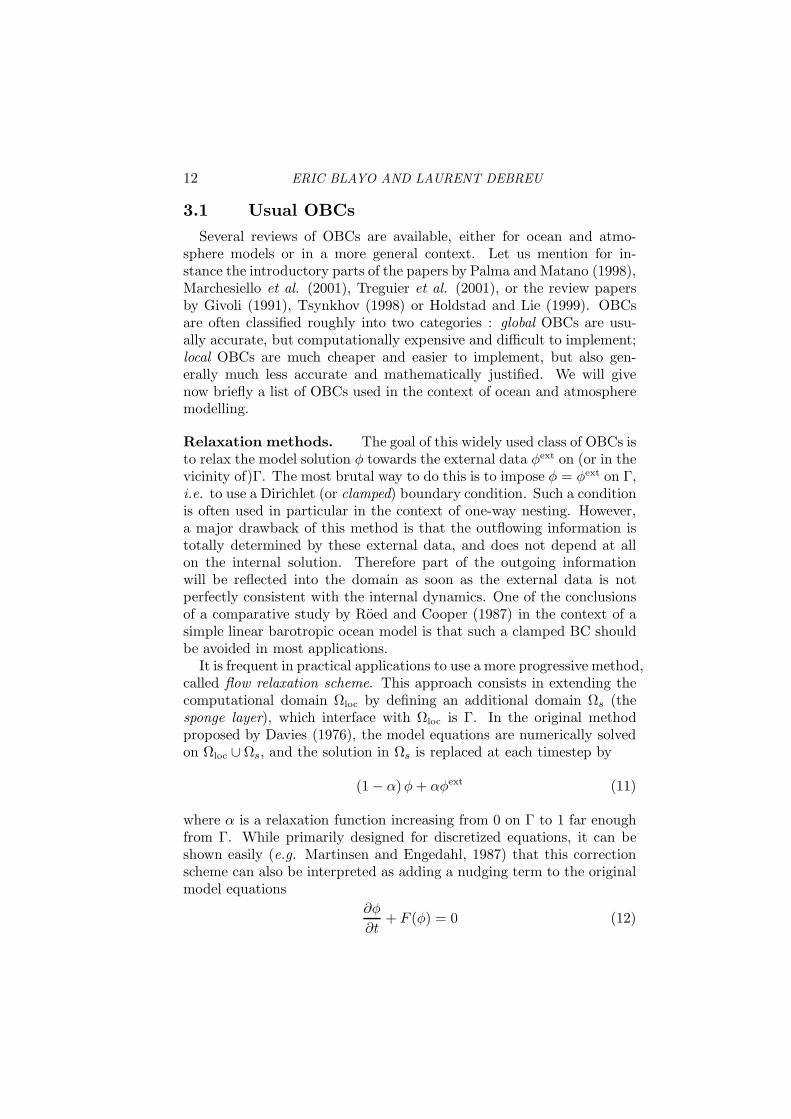
Let us now illustrate the different preceding approaches in the verysimple case of a 1-D ordinary differential equation. The problem is :

−ν(x)u′′(x) + u(x) = sin nπx x ∈]0, 1[u(0) = u(1) = 0

(9)

The local domain we are interested in is Ωloc =]a, b[; hence Ωext =]0, a[∪]b, 1[. ν(x) is displayed on Figure 2a. It is equal to ν0 in Ωext, and


ν0/√

2 in Ωloc, except in two small transition zones of width δ, whereit varies smoothly between ν0 and ν0/

√2. This problem has a unique

solution (Brezis, 1983), denoted uref , which is plotted on Figure 2b.The elliptic nature of this problem amplifies the influence of the bound-ary conditions, which will help highlighting the differences between thenesting approaches described in §2.

Open boundary problem. Solve −ν(x)u′′

obc(x)+uobc(x) = sinnπx,x ∈]a, b[, with OBCs at a and b. Such OBCs can be for exampleDirichlet conditions uobc(a) = α0, uobc(b) = β0, or Neumann conditionsu′

obc(a) = α1, u′

obc(b) = β1. If the external data are perfect ( [α0, β0] =[uref (a), uref (b)] or [α1, β1] = [u′

ref (a), u′

ref (b)] ) then we get the true so-lution uref . We have plotted in Figure 2b the case of imperfect Dirichletdata α0 = β0 = 0.

One-way / two-way nesting. Since the problem is not time de-pendent, both one-way and two-way approaches yield the same solutionunes, defined by :

−ν0 u′′

ext(x) + uext(x) = sin nπx, x ∈]0, 1[uext(0) = uext(1) = 0

−ν(x)u′′

nes(x) + unes(x) = sin nπx, x ∈]a, b[Baunes(a) = Bauext(a) and Bbunes(b) = Bbuext(b)

(10)

We have plotted in Figure 2b the cases Ba = Bb = Id and Ba = Bb =∂/∂n. As can be seen clearly, these methods, which are all supposed toapproximate the true problem (9), yield quite different solutions, whichcan differ from uref both in Ωloc and Ωext. Note also that the trueproblem (9), reformulated as (5), requires two BCs at a and b, while theapproximate formulations require only one BC.

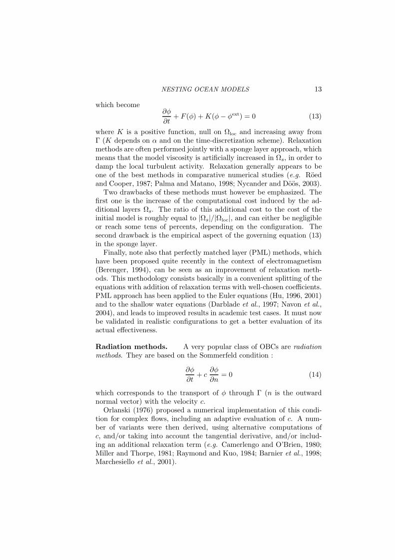
The same type of comparison is displayed in Figure 3, but for therealistic testcase of a high resolution model of the bay of Biscay coupledwith an eddy-permitting model of the North Atlantic.

3. The open boundary problem

Let us now focus on the main point, central in all approaches, namelythe choice of the open boundary operators B in (6)-(7)-(8). This is adifficult problem, which has been the subject of numerous studies formore than 30 years, ranging from purely mathematical approaches tospecific modelling applications. Mathematical results are often obtainedfor simplified equations (e.g. linearized and/or inviscid). They generallyaddress the derivation of OBCs, and the well-posedness of the modelequations using these OBCs. Note that the well-posedness of the system


0 0.1 0.2 0.3 0.4 0.5 0.6 0.7 0.8 0.9 10.1

0.15

0.2

0.25

0.3

0.35

0.4

0 0.1 0.2 0.3 0.4 0.5 0.6 0.7 0.8 0.9 1−0.05

−0.04

−0.03

−0.02

−0.01

0

0.01

0.02

0.03

0.04

0.05

Figure 2. a) ν(x) for eq.(9); b) The different solutions (see text) : uref (solid line),uobc (thick solid line), unes with Dirichlet and Neumann OBCs (dashed lines). Thetwo vertical lines correspond to x = a and x = b.

1

Figure 3. Averaged temperature at z = 30m in spring 1998, in a 1/15regional modelof the bay of Biscay interacting with a 1/3model of the north Atlantic. The internalrectangle corresponds to the limits of the regional model. The model of the northAtlantic is only partially shown. Three interactions procedures are compared (fromS. Cailleau, 2004).

ensures the uniqueness of the solution and its stability with regard toinitial datum, but does not give any information on its accuracy norrelevance with regard to the “true” solution uref . On the other hand,numerical studies can use complex realistic models, but their results seemoften dependent on the test cases. We present here a brief overviewof usual OBCs, and give a tentative explanation of their performancethrough the point of view of hyperbolic systems. The contents of thissection is discussed in much more details in Blayo and Debreu (2005).


3.1 Usual OBCs

Several reviews of OBCs are available, either for ocean and atmo-sphere models or in a more general context. Let us mention for in-stance the introductory parts of the papers by Palma and Matano (1998),Marchesiello et al. (2001), Treguier et al. (2001), or the review papersby Givoli (1991), Tsynkhov (1998) or Holdstad and Lie (1999). OBCsare often classified roughly into two categories : global OBCs are usu-ally accurate, but computationally expensive and difficult to implement;local OBCs are much cheaper and easier to implement, but also gen-erally much less accurate and mathematically justified. We will givenow briefly a list of OBCs used in the context of ocean and atmospheremodelling.

Relaxation methods. The goal of this widely used class of OBCs isto relax the model solution φ towards the external data φext on (or in thevicinity of)Γ. The most brutal way to do this is to impose φ = φext on Γ,i.e. to use a Dirichlet (or clamped) boundary condition. Such a conditionis often used in particular in the context of one-way nesting. However,a major drawback of this method is that the outflowing information istotally determined by these external data, and does not depend at allon the internal solution. Therefore part of the outgoing informationwill be reflected into the domain as soon as the external data is notperfectly consistent with the internal dynamics. One of the conclusionsof a comparative study by Roed and Cooper (1987) in the context of asimple linear barotropic ocean model is that such a clamped BC shouldbe avoided in most applications.

It is frequent in practical applications to use a more progressive method,called flow relaxation scheme. This approach consists in extending thecomputational domain Ωloc by defining an additional domain Ωs (thesponge layer), which interface with Ωloc is Γ. In the original methodproposed by Davies (1976), the model equations are numerically solvedon Ωloc ∪ Ωs, and the solution in Ωs is replaced at each timestep by

(1 − α)φ + αφext (11)

where α is a relaxation function increasing from 0 on Γ to 1 far enoughfrom Γ. While primarily designed for discretized equations, it can beshown easily (e.g. Martinsen and Engedahl, 1987) that this correctionscheme can also be interpreted as adding a nudging term to the originalmodel equations

∂φ

∂t+ F (φ) = 0 (12)


which become∂φ

∂t+ F (φ) + K(φ − φext) = 0 (13)

where K is a positive function, null on Ωloc and increasing away fromΓ (K depends on α and on the time-discretization scheme). Relaxationmethods are often performed jointly with a sponge layer approach, whichmeans that the model viscosity is artificially increased in Ωs, in order todamp the local turbulent activity. Relaxation generally appears to beone of the best methods in comparative numerical studies (e.g. Roedand Cooper, 1987; Palma and Matano, 1998; Nycander and Doos, 2003).

Two drawbacks of these methods must however be emphasized. Thefirst one is the increase of the computational cost induced by the ad-ditional layers Ωs. The ratio of this additional cost to the cost of theinitial model is roughly equal to |Ωs|/|Ωloc|, and can either be negligibleor reach some tens of percents, depending on the configuration. Thesecond drawback is the empirical aspect of the governing equation (13)in the sponge layer.

Finally, note also that perfectly matched layer (PML) methods, whichhave been proposed quite recently in the context of electromagnetism(Berenger, 1994), can be seen as an improvement of relaxation meth-ods. This methodology consists basically in a convenient splitting of theequations with addition of relaxation terms with well-chosen coefficients.PML approach has been applied to the Euler equations (Hu, 1996, 2001)and to the shallow water equations (Darblade et al., 1997; Navon et al.,2004), and leads to improved results in academic test cases. It must nowbe validated in realistic configurations to get a better evaluation of itsactual effectiveness.

Radiation methods. A very popular class of OBCs are radiation

methods. They are based on the Sommerfeld condition :

∂φ

∂t+ c

∂φ

∂n= 0 (14)

which corresponds to the transport of φ through Γ (n is the outwardnormal vector) with the velocity c.

Orlanski (1976) proposed a numerical implementation of this condi-tion for complex flows, including an adaptive evaluation of c. A num-ber of variants were then derived, using alternative computations ofc, and/or taking into account the tangential derivative, and/or includ-ing an additional relaxation term (e.g. Camerlengo and O’Brien, 1980;Miller and Thorpe, 1981; Raymond and Kuo, 1984; Barnier et al., 1998;Marchesiello et al., 2001).


Such radiation methods are frequently used in ocean and atmospheremodelling. However their relevance for such complex flows is far fromobvious. Their reputation is split : they have proved to give rather poorresults in several comparative studies (e.g. Roed and Cooper, 1987;Palma and Matano, 1998; Nycander and Doos, 2003), while they seemto have some efficiency in others (e.g. Marchesiello et al., 2001; Treguieret al., 2001). In fact the Sommerfeld condition is justified only in thecontext of wave equations with a constant phase velocity (Blayo andDebreu, 2005). Applying such a condition to variables which do notsatisfy at all such equations results in a fundamental nonlinearity, whichhas been recently pointed out by Nycander and Doos (2003). Thereforethis condition cannot be mathematically justified in the context of oceanand atmosphere modelling. However, its actual implementations give animportant role to external data. As indicated previously, the radiationvelocity c is evaluated at each timestep and at each gridpoint on theopen boundary. If c is inward, the model variable is generally set to thecorresponding external value: φ = φext, or strongly relaxed towards it:

∂φ

∂t= − φ − φext

τin

(15)

where τin is a short relaxation timescale. If c is outward, then the ra-diation equation is applied, but often with the addition of a relaxationterm :

∂φ

∂t+ c

∂φ

∂n= − φ − φext

τout

(16)

where τout is a longer relaxation timescale. In their careful analysis of asimulation of the Atlantic ocean, Treguier et al. (2001) have observedthat c behaves in some sense like a white noise, and is directed inwardsabout half of the time at any location on the open boundaries. Thereforethe model solution at the open boundary never departs significantlyfrom the external data, and the radiation condition acts in fact nearlyas a clamped condition. So it is probably the strong influence of theexternal data through the additional relaxation term in the radiationconditions that gives them most of their practical efficiency, rather thanthe radiation procedure.

Flather condition. Flather (1976) proposed an OBC for 2-Dbarotropic flows, which is often classified within the family of radiationconditions. This condition can be obtained by combining the Sommer-feld condition for the surface elevation η (with surface gravity wavesphase speed)

∂η

∂t+

√

gh∂η

∂n= 0 (17)


with a one-dimensional approximation of the continuity equation

∂η

∂t+ h

∂vn

∂n= 0 (18)

where g is the gravity, h is the local water depth and vn is the normalcomponent of the barotropic velocity. Substracting (17) to (18) andintegrating through Γ, one obtains:

vn −√

g

hη = vext

n −√

g

hηext (19)

The Flather condition has been used in several comparative studies (e.g.Palma and Matano, 1998; Marchesiello et al., 2001; Nycander and Doos,2003), and it always appears to be one of the most efficient conditions.

Model adapted methods. A striking aspect of radiation andrelaxation methods is that the OBCs do not depend on the model equa-tions. On the opposite, other methods provide OBCs which are adaptedto the system. However, since they are more complicated to handle,the use of such methods is quite rare and restricted to simple 1-D or2-D models, and has never been extended to our knowledge to realisticprimitive equations systems.

This is the case of characteristic waves amplitudes methods(sometimes called Hedstrom methods), designed for hyperbolic systems.The basic idea consists in choosing for OBCs the original set of modelequations with as few approximations as possible. Since the only quanti-ties that cannot be evaluated by the model alone are the incoming char-acteristics (see §3.2) the approximations must concern only these terms,and eventually the viscous terms if the model is not inviscid. This resultsin setting to zero (or to a value deduced from external data) the normalderivative of the incoming characteristic variables on Γ. Several papersdeveloped this idea these last years in the context of direct numericalsimulation of compressible Euler and Navier-Stokes equations, with ap-parently good experimental results (Poinsot and Lele, 1992; Bruneau,2000; Bruneau and Creuse, 2001). In the context of ocean modelling, itis compared to other OBCs by Roed and Cooper (1987), Jensen (1998)and Palma and Matano (1998), and leads to rather good results.

Another important family of methods are absorbing conditions,which are exact relations satisfied by the outgoing quantities at the openboundary. In a reference paper, Engquist and Majda (1977) give a gen-eral method for obtaining such relations, using time and space Fouriertransforms. However, these conditions are generally global in time andspace, and cannot be used just as it is in practice. That is why they


must be approximated to give tractable local conditions. A strong in-terest of this approach is its sound mathematical foundation, and itspractical efficiency in several domains of applications. Several papershave recently readdressed the derivation of absorbing BCs for the invis-cid shallow water system, and obtain apparently quite good numericalresults (Lie, 2001; McDonald, 2002, 2003; Nycander and Doos, 2003).

3.2 An hyperbolic point of view

When attempting to draw some synthesis of the numerous previousstudies on OBCs, two keypoints stand out, which seem to be necessaryconstituents for any good OBC. The first point is that good results areobtained when taking primarily into account the hyperbolic part of thedynamics, and therefore when working on incoming characteristic vari-ables. The second point is that this must be associated with a consistentuse of some external data.

Incoming characteristic variables. Let us first introduce somestandard definitions concerning hyperbolic systems. The general formof such a system is

∂Φ

∂t+ A(Φ)

∂Φ

∂x= F (20)

where Φ(x, t) is a vector of n functions, A(Φ) is a n × n matrix offunctions of Φ, and F is a forcing term. For the system to be hyperbolic,A must have n real eigenvalues and n distinct eigenvectors. Let Wk

the kth left eigenvector of A, corresponding to the kth eigenvalue λk :W T

k A = λk W Tk . Multipliying (20) on the left by W T

k , one gets:

W Tk

dkΦ

dt= W T

k F withdk

dt=

(

∂

∂t+ λk

∂

∂x

)

(21)

The operator dk/dt represents a total (or directional) derivative in the di-

rection defined bydx

dt= λk. To the hyperbolic system (20) correspond n

such families of curves, which are called characteristic curves of the sys-tem. If the system (20) is linear with constant coefficients, i.e. if A is aconstant matrix, one can define the new variables wk(x, t) = W T

k Φ(x, t).(20) is then equivalent to the system of n uncoupled transport equations:

∂wk

∂t+ λk

∂wk

∂x= W T

k F k = 1, . . . , n (22)

The characteristic curves in that case are the lines x − λkt = constant,along which the wk (called characteristic variables or Riemann invari-

ants) are conserved. One can notice that, at a given boundary, these


characteristic variables will be either inflowing or outflowing, dependingon the sign of λk.

A fundamental point is that, for a hyperbolic open boundary problemto be well-posed, one must prescribe as many boundary conditions as thenumber of incoming characteristics. This result is in fact quite intuitive: the solution can be decomposed into outgoing and incoming charac-teristics; information on the former is available within the computationdomain, and no additional condition is required, while information onthe latter is not available, and mustbe specified.

Consistency with external data. The second keypoint concernsthe connection with external data. It appears that a reasonable choiceconsists in imposing the consistency locally all along the boundary. Thismeans that the OBC is of the form

Bφ = Bφext (23)

where B is the open boundary operator. B = Id corresponds to thecontinuity of φ through the boundary, and B = ∂/∂n to the continuityof the flux. Such a formulation (23) is quite natural for example if weconsider that the external data φext represents some steady state or farfield solution φ∞. In that case, as detailed for example by Engquist andHalpern (1988), if we want the model solution to converge to the steadystate solution as t → ∞, then the OBC must also be satisfied by φ∞.

Used together with the point of view of characteristic variables pre-sented previously, this condition (23) leads to recommending OBCs ofthe form

Bw = Bwext (24)

where w is any incoming characteristic variable of the governing equa-tions.

The extension to non-hyperbolic systems, like for example the Navier-Stokes equations, is not trivial. A logical approximation consists howeverin considering only the hyperbolic part of thesystem, and to use the sameprocedures as for the hyperbolic case.

Revisiting usual OBCs. The preceding criteria give a new lighton usual OBCs. It appears indeed that :

the Sommerfeld condition (14) corresponds to prescribing to zerothe incoming characteristic of the wave equation. That is why itis legitimate for wave equations but not for other systems.


the Flather condition (14) corresponds to specifying the value ofthe incoming characteristic of the shallow water system, fulfillingthe criterion (24) with B = Id the identity operator.

absorbing conditions are closely linked to incoming characteristicvariables, and the conditions proposed by McDonald (2002, 2003)and Nycander and Doos (2003) can be written under the form (24).

characteristic waves amplitudes methods do also meet the preced-ing point of view.

since relaxation methods are not local conditions, the criterion(24) does not apply directly. However, it is obvious from (11) thatthe transition from φ to φext is smooth as soon as the additionaldomain Ωs is large enough. Similarly the problem of specifyingincoming characteristics and evacuating outcoming characteristicsat the open boundary is treated implicitely : the values of theincoming characteristics are computed within Ωs, using the relaxedsolution, while the outgoing characteristics are not directly affectedwhen reaching Γ but are relaxed in Ωs towards their correspondingexternal values, and damped by the increased dissipation.

Details on these aspects, as well as an application of the criterion (24) toshallow-water and primitive equations systems, are discussed in Blayoand Debreu (2005).

3.3 Some practical remarks

It is important to note that we discussed here only the continuousform of the equations. However discretized models contain spuri-ous numerical modes, which nature is different from that of phys-ical modes, and which have to be handled by the OBCs. There-fore, once the continuous form of the OBCs is chosen, one hasto perform some specific work in order to adapt their numericalimplementation to the numerical schemes of the model. This diffi-culty is probably also a reason for the efficiency of relaxation andradiation-relaxation methods, which tend to automatically dampthese non-physical modes.

Incoming information is entirely given by the external solution φext.Therefore the quality of these data is of course an important pointin the performance of a regional modelling system.

Another important practical aspect in a regional modelling systemis the initialization problem. The initial condition is generally built


by interpolation of a larger scale solution, which is not perfectlyconsistent with the local model. This can yield an adjustmentphase which can be quite long, and which pollutes the model solu-tion. A way to avoid (or limit) this problem is to add some relevantconstraints in the computation of the initial condition, as done forinstance by Auclair et al. (2000) using an inverse approach. Thisaspect is presently the subject of numerous studies.

4. Two-way interaction

4.1 Two-way nesting

As explained in §2, the usual two-way method differs from the pre-ceding one-way method by the addition of an update procedure. Thissupplementary step aims at improving uext by modifying it locally usinguloc. This retroaction from the local model onto the external model isperformed every external model timestep, or less frequently. The updateoperator generally replaces the values of uext at gridpoints located in Ωloc

by copying the corresponding values of uloc, eventually after some timeand space averaging. Such an update is quite brutal, and in particulardoes not ensure the balance of mass and tracers fluxes through Γ. For

example,

∫

ΓUloc.n 6=

∫

ΓUext.n, where U denotes the velocity. That is

why a flux correction step is often added, which generally modifies uloc

to distribute the flux misfit all along Γ, to get finally a local solution u∗

loc

which is in flux balance with uext.The two-way method generally decreases the difficulties that can be

encountered by the one-way method (in particular the instabilities alongΓ), and seems to improve the model solution. That is why it is recom-mended to use it as far as possible rather than one-way interaction.However, it is clear that the solution provided by this usual two-waynesting is not solution of the original problem (5): before the flux cor-rection step, the connection between uext and uloc is not differentiable,because their fluxes are not balanced; after the flux correction step, theconnection is no more continuous because uloc has been modified intou∗

loc, which in addition does not satisfy any longer the local model equa-

tions (1).

4.2 Full coupling - Schwarz methods

Obtaining a solution of the original problem (5) is much more difficultand expensive than what is done in the above usual algorithms. This ismainly due to the fact that, since the local and external model equationsare different, their domains of application should not overlap. Therefore


the external model, which is generally available in a configuration fullyoverlapping Ωloc, must be modified to add an open boundary. Moreover,once this is done, one has to find and implement an algorithm ensur-ing that the solutions uext and uloc will satisfy the desired regularityconditions through Γ.

These difficulties explain that this problem has never been addressedbefore in ocean and atmosphere modelling. This can be done howeverwithin the mathematical framework of domain decomposition methods.These methods have been intensively studied and developed since theend of the eighties due to the advent of parallel computers. With-out going into details, let us present the global-in-time non-overlapping

Schwarz algorithm, which seems well suited for our ocean coupling prob-lem. This iterative algorithm can be written as follows :

Llocun+1loc = floc in Ωloc × [0, T ]

un+1loc given at t = 0

Blocun+1loc = Blocu

next on Γ × [0, T ]

and

Lextun+1ext = fext in Ωext × [0, T ]

un+1ext given at t = 0

Bextun+1ext = Bextu

nloc on Γ × [0, T ]

(25)

where the superscripts denote the number of iterations, and Bloc andBext are interface operators to be chosen. Note that, at each iteration,the two models can be run in parallel over the whole time window [0, T ].If no parallel computer is available, the interface condition for uext canbe replaced for example by Bextu

n+1ext = Bextu

n+1loc , which prevents paral-

lelism but increases the convergence rate of the algorithm.This rate closely depends of the choice of Bloc and Bext. An obvi-

ous possibility is to choose the operators Id and ∂/∂n. Therefore, oncethe algorithm has converged, its solution will satisfy (5). However theconvergence can be quite slow and, given the computational burden ofocean models, one probably cannot afford numerous iterations of suchan algorithm. That is why the choice of the interface operators must beoptimized. A simple but quite efficient possibility is to use Robin con-ditions : Bloc = ∂/∂n + rlocId and Bext = ∂/∂n + rextId with rloc 6= rext.This ensures the desired regularity as previously for the converged so-lution, but a good choice of the coefficients rloc and rext can greatlyspeed up the convergence. More sophisticated approaches can be usedto determine good interface operators, which are closely linked to charac-teristic methods and absorbing conditions. Martin (2003) applied suchapproaches to 2-D tracer equations and to the shallow-water system.She derived very efficient operators, which ensure the convergence of the


algorithm in some very few iterations. Development of such algorithmsfor realistic ocean models is ongoing research work.

5. Software tools

Designing nested or coupled systems starting from existing modelsis quite a difficult and time-consuming practical task. However severalsoftware tools have been developed these last years, which automaticallymanage an important part of the job.

The AGRIF package1 (Debreu et al., 2004a) allows an easy integra-tion of mesh refinement capabilities within any existing finite-differencemodel written in Fortran. One can therefore design one-way and two-way multiply-nested systems, with the possibility of adaptive regridding,without reprogramming the model. This package is presently imple-mented into several operational ocean models.

General couplers can also be used to implement nested systems, es-pecially in the case when the local and external model codes are totallydifferent. The user has then to prescribe the structure of the couplingalgorithm and the interactions between the different objects, but at arather high level, without having to go too much into programmingdetails. In the context of geophysical fluids, we can cite for instancePALM2 or MpCCI3.

6. Data assimilation and nesting

Along with the development of nested ocean modelling systems, theproblem of assimilating data within these systems is presently stronglyemerging. Addressing this difficult problem is out of the scope of thisnote. Let us however point out a few related issues.

The exact mathematical formulation of the data assimilation prob-lem for one-way or two-way nested systems is far from obvious. Afirst attempt in this direction for the 4D-Var approach can befound in Debreu et al. (2004b). Concerning the stochastic ap-proach, interesting ideas can probably be found in the theories ofmultiresolution stochastic models and multiscale estimation.

Several ad-hoc procedures are already in use in numerous systems.A possibility is to perfom the assimilation only on one grid (thelargest or the finest) of the system. Another way is to ”hide” the

1http://www-lmc.imag.fr/IDOPT/AGRIF2http://www.cerfacs.fr/~palm3http://www.mpcci.org


grid interaction process and to make the assimilation globally ona multiresolution state vector (e.g. Barth et al., 2004).

It is possible in a variational method to manage simultaneously thecoupling problem and the assimilation problem. See for instanceBounaim (1999) or Taillandier et al.(2004).

In a multiresolution modelling system, one has to choose whichdata are assimilated on which grid. Since the model dynamicsdepends on the grid resolution, and since the data themselves haveoften been collected or processed with some spatial and temporalresolution, this choice is not obvious and has consequences on thequality of the identified solution.

References

Auclair, F., S. Casitas, and P. Marsaleix, 2000: Application of an inverse method tocoastal modelling. J. Atmos. Oceanic Technol., 17, 1368–1391.

Barnier, B., P. Marchesiello, A.P. de Miranda, J.M. Molines, and M. Coulibaly, 1998:A sigma coordinate primitive equation model for studying the circulation in theSouth Atlantic I, Model configuration with error estimates. Deep Sea Res., 45,543–572.

Barth, A., A. Alvera-Azcarate, J.-M. Beckers, M. Rixen, L. Vandenbulke and Z. BenBouallegue, 2004: Multigrid state vector for data assimilation in a two-way nestedmodel of the Ligurian sea. 36th International Liege Colloquium on Ocean Dynam-

ics.Bennett, A.F., 2002: Inverse modeling of the ocean and atmosphere. Cambridge Uni-

versity Press, 2002.Berenger, J.-P., 1994: A perfectly matched layer for the absorption of electromagnetic

waves. J. Comput. Phys., 114, 185–200.Blayo, E., and L. Debreu, 2005: Revisiting open boundary conditions from the point

of view of characteristic variables. Ocean Modelling, 9, 231–252..Bounaim, A., 1999: Methodes de decomposition de domaine: application a la resolution

de problemes de controle optimal. PhD thesis, Universite Grenoble 1.Brezis, H., 1983: Analyse fonctionnelle. Masson.Bruneau, C.-H., 2000: Boundary conditions on artificial frontiers for incompressible

and compressible Navier-Stokes equations. Math. Mod. and Num. Anal., 34, 303–314.

Bruneau, C.H., and E. Creuse, 2001: Towards a transparent boundary condition forcompressible Navier-Stokes equations. Int. J. Numer. Meth. Fluids, 36, 807–840.

Cailleau, S., 2004: Validation de methodes de contrainte aux frontieres d’un modeleoceanique : application a un modele hauturier de l’Atlantique Nord et a un modeleregional du Golfe de Gascogne. PhD thesis, Universite Grenoble 1.

Camerlengo, A.L., and J.J. O’Brien, 1980: Open boundary conditions in rotatingfluids. J. Comp. Phys., 35, 12–35.

Darblade, G., R. Baraille, A.-Y. Le Roux, X. Carton, and D. Pinchon, 1997: Condi-tions limites non reflechissantes pour un modele de Saint-Venant bidimensionnelbarotrope linearise. C.R. Acad. Sci. Paris, Serie 1, 324, 485–490.


Davies, H.C., 1976: A lateral boundary formulation for multi-level prediction models.Quart. J. R. Meteorol. Soc., 102, 405–418.

Debreu, L., C. Vouland and E. Blayo, 2004a: AGRIF: Adaptive Grid Refinement inFortran. To appear in Computers and Geosciences.

Debreu, L., Y. De Visme and E. Blayo, 2004b: 4D Variational data assimilation forlocally nested models. In preparation.

Engquist, B., and A. Majda, 1977: Absorbing boundary conditions for the numericalsimulation of waves. Math. Comp., 31, 629–651.

Engquist, B., and L. Halpern, 1988: Far field boundary conditions for computationoverlong time. Appl. Num. Math., 4, 21–45.

Flather, R.A., 1976: A tidal model of the north-west European continental shelf. Mem.

Soc. R. Sci. Liege, 6(10), 141–164.Givoli, D., 1991: Non-reflecting boundary conditions. J. Comp. Phys., 94, 1–29.Hedstrom, G.W., 1979: Nonreflecting boundary conditions for nonlinear hyperbolic

system. J. Comp. Phys., 30, 222–237.Holstad, A., and I. Lie, 1999: On transparent boundary conditions and nesting for

ocean models. Research report 91, Norwegian Meteorological Institute, Oslo, Nor-way.

Hu, F. Q., 1996: On absorbing boundary conditions for linearized Euler equations bya perfectly matched layer. J. Comp. Phys., 129, 201–219.

Hu, F. Q., 2001: A stable perfectly matched layer for linearized Euler equations inunsplit physical variables. J. Comp. Phys., 173, 455–480.

Jensen, T., 1998: Open boundary conditions in stratified ocean models. J. Mar. Sys.,16, 297–322.

Lie, I., 2001: Well-posed transparent boundary conditions for theshallow water equa-tions. App. Num. Math., 38, 445-474.

Marchesiello, P., J. McWilliams, and A. Shchepetkin, 2001: Open boundary conditionsfor long-term integration of regional oceanic models. Ocean Modelling, 3, 1–20.

Martin, V., 2003: Methodes de decomposition de domaine de type relaxation d’ondespour des equations de l’oceanographie. PhD thesis, Universite Paris 13.

Martinsen, E.A., and H.E. Engedahl, 1987: Implementation and testing of a lateralboundary scheme as an open boundary condition in a barotropic ocean model.Coastal Eng., 11, 603–627.

McDonald, A., 2002: A step toward transparent boundary conditions for meteorolog-ical models. Mon. Weath. Rev., 130, 140–151.

McDonald, A., 2003: Transparent boundary conditions for the shallow water equa-tions: testing in a nested environment. Mon. Weath. Rev., 131, 698–705.

Miller, M.J., and A.J. Thorpe, 1981: Radiation conditions for the lateral boundariesof limited-area numerical models. Quart. J. R. Meteorol. Soc., 107, 615–628.

Navon, I.M., B. Neta, and M.Y. Hussaini, 2004: A perfectly matched layer approach tothe linearized shallow water equations models: the split equation approach. Mon.

Weather Rev., 132, 1369–1378.Nycander, J., and K. Doos, 2003: Open boundary conditions for barotropic waves. J.

Geophys. Res., 108(C5), 3168–3187.Orlanski, I., 1976: A simple boundary condition for unbounded hyperbolic flows. J.

Comp. Phys., 21, 251–269.Palma, E.D., and R.P. Matano, 1998: On the implementation of passive open bound-

ary conditions for a general circulation model: the barotropic mode. J. Geophys.

Res., 103(C1), 1319–1341.


Poinsot, T., and S.K. Lele, 1992: Boundary conditions for subsonic Navier-Stokescalculations. J. Comp. Phys., 101, 104-129.

Raymond, W.H., and H.L. Kuo, 1984: A radiation boundary condition for multi-dimensional flows. Quart. J. R. Met. Soc., 110, 535–551.

Roed, L.P., and C. Cooper, 1987: A study of various open boundary conditions forwind-forced barotropic numerical ocean models, in Three-dimensional models of

marine andestuarine dynamics, edited by J.C.J. Nihoul and B.N. Jamart, pp. 305–335, Elsevier.

Taillandier, V., V. Echevin, L. Mortier and J.-L. Devenon, 2004: Controlling boundaryconditions with a four-dimensional variational data assimilation method in a non-stratified open coastal model. Ocean Dyn., 54, 284–298.

Treguier, A.-M., B. Barnier, A.P. de Miranda, J.-M. Molines, N. Grima, M. Imbard,G.Madec, and C. Messager, 2001: An eddy permitting model of the Atlantic cir-culation: evaluating openboundary conditions. J. Geophys. Res, 106(C10), 22115–22130.

Tsynkhov, S.V., 1998: Numerical solutions of problems on unbounded domains. Areview. Appl. Numer. Math., 27, 456–532.

Documents

Eric Blayo, Laurent Debreu To cite this version - … · 6 ERIC BLAYO AND LAURENT DEBREU 2. A classiﬁcation of nesting problems 2.1 General framework We are interested in representing