Centre de Recherches MathematiquesCRM Proceedings and Lecture NotesVolume ??, 2007

Ergodic Methods in Additive Combinatorics

Bryna Kra

Abstract. Shortly after Szemeredi’s proof that a set of positive upper densitycontains arbitrarily long arithmetic progressions, Furstenberg gave a new proofof this theorem using ergodic theory. This gave rise to the field of combinato-rial ergodic theory, in which problems motivated by additive combinatorics areaddressed kwith ergodic theory. Combinatorial ergodic theory has since pro-duced combinatorial results, some of which have yet to be obtained by othermeans, and has also given a deeper understanding of the structure of measurepreserving systems. We outline the ergodic theory background needed to un-derstand these results, with an emphasis on recent developments in ergodictheory and the relation to recent developments in additive combinatorics.

These notes are based on four lectures given during the School on AdditiveCombinatorics at the Centre de recherches mathematiques, Montreal in April,2006. The talks were aimed at an audience without background in ergodictheory. No attempt is made to include complete proofs of all statements andoften the reader is referred to the original sources. Many of the proofs includedare classic, included as an indication of which ingredients play a role in thedevelopments of the past ten years.

1. Combinatorics to ergodic theory

1.1. Szemeredi’s theorem. Answering a long standing conjecture of Erdosand Turan [11], Szemeredi [54] showed that a set E ⊂ Z with positive upper density1

contains arbitrarily long arithmetic progressions. Soon thereafter, Furstenberg [16]gave a new proof of Szemeredi’s Theorem using ergodic theory, and this has lead tothe rich field of combinatorial ergodic theory. Before describing some of the resultsin this subject, we motivate the use of ergodic theory for studying combinatorialproblems.

We start with the finite formulation of Szemeredi’s theorem:

Theorem 1.1 (Szemeredi [54]). Given δ > 0 and k ∈ N, there is a functionN(δ, k) such that if N > N(δ, k) and E ⊂ {1, . . . , N} is a subset with |E| ≥ δN ,then E contains an arithmetic progression of length k.

1991 Mathematics Subject Classification. Primary 37A30; Secondary 11B25, 27A45.Key words and phrases. Ergodic theory, additive combinatorics.The author was supported in part by NSF Grant DMS-#0555250.This is the final form of the paper.1Given a set E ⊂ Z, its upper density d∗(E) is defined by d∗(E) = lim supN→∞ |E ∩

{1, . . . , N}|/N .

c©2007 American Mathematical Society

1

2 B. KRA

It is clear that this statement immediately implies the first formulation of Sze-meredi’s theorem, and a compactness argument gives the converse implication.

1.2. Translation to a probability system. Starting with Szemeredi’s the-orem, one gains insight into the intersection of sufficiently many sets with positivemeasure in an arbitrary probability system.2 Note that N(δ, k) denotes the quantityin Theorem 1.1.

Corollary 1.2. Let δ > 0, k ∈ N, (X,X , µ) be a probability space and A1, . . . ,AN ∈ X with µ(Ai) ≥ δ for i = 1, . . . , N . If N > N(δ, k), then there exist a, d ∈ Nsuch that

Aa ∩Aa+d ∩Aa+2d ∩ · · · ∩Aa+kd 6= ∅.

Proof. For A ∈ X , let 1A(x) denote the characteristic function of A (meaningthat 1A(x) is 1 for x ∈ A and is 0 otherwise). Let N > N(δ, k). Then

∫

X

1N

N−1∑n=0

1An dµ ≥ δ.

Thus there exists x ∈ X such that

1N

N−1∑n=0

1An(x) ≥ δ.

Then E = {n : x ∈ An} satisfies |E| ≥ δN , and so Szemeredi’s theorem impliesthat E contains an arithmetic progression of length k. By the definition of E, wehave a sequence of sets with the desired property. ¤

1.3. Measure preserving systems. A probability measure preserving systemis a quadruple (X,X , µ, T ), where (X,X , µ) is a probability space and T : X → Xis a bijective, measurable, measure preserving transformation. This means that forall A ∈ X , T−1A ∈ X and

µ(T−1A) = µ(A).

In general, we refer to a probability measure preserving system as a system.Without loss of generality, we can place several simplifying assumptions on

our systems. We assume that X is countably generated; thus for 1 ≤ p < ∞,Lp(µ) is separable. We implicitly assume that all sets and functions are measurablewith respect to the appropriate σ-algebra, even when this is not explicitly stated.Equality between sets or functions is always meant up to sets of measure 0.

2A σ-algebra is a collection X of subsets of X satisfying: (i) X ∈ X (ii) for any A ∈ X wealso have X \ A ∈ X (iii) for any countable collection An ∈ X , we also have

S∞n=1 An ∈ X . A

σ-algebra is endowed with operationsW

,V

, and c, which correspond to union, intersection, andtaking complements. By a probability system, we mean a triple (X,X , µ) where X is a measurespace, X is a σ-algebra of measurable subsets of X, and µ is a probability measure. In general,we use the convention of denoting the σ-algebra X by the associated calligraphic version of themeasure space X.

ERGODIC METHODS IN ADDITIVE COMBINATORICS 3

1.4. Furstenberg multiple recurrence. In a system, one can use Szeme-redi’s theorem to derive a bit more information about intersections of sets. If(X,X , µ, T ) is a system and A ∈ X with µ(A) ≥ δ > 0, then

A, T−1A, T−2A, . . . , T−nA, . . .

are all sets of the same measure, and so all have measure ≥ δ. Applying Corol-lary 1.2 to this sequence of sets, we have the existence of a, d ∈ N with

T−aA ∩ T−(a+d)A ∩ T−(a+2d) ∩ · · · ∩ T−(a+kd)A 6= ∅.

Furthermore, the measure of this intersection must be positive. If not, we couldremove from A a subset of measure zero containing all the intersections and obtaina subset of measure at least δ without this property. In this way, starting withSzemeredi’s Theorem, we have derived Furstenberg’s multiple recurrence theorem:

Theorem 1.3 (Furstenberg [16]). Let (X,X , µ, T ) be a system and let A ∈ Xwith µ(A) > 0. Then for any k ≥ 1, there exists n ∈ N such that

(1.1) µ(A ∩ T−nA ∩ T−2nA ∩ · · · ∩ T−knA

)> 0.

2. Ergodic theory to combinatorics

2.1. Strong form of multiple recurrence. We have seen that Fursten-berg multiple recurrence can be easily derived from Szemeredi’s theorem. Moreinteresting is the converse implication, showing that one can use ergodic theoryto prove regularity properties of subsets of the integers, and in particular deriveSzemeredi’s theorem. This is what Furstenberg did in his landmark paper [16],and the techniques introduced in this paper have been used subsequently to deduceother patterns in subsets of integers with positive upper density. (See Section 9.)Moreover, Furstenberg’s proof lead to new questions within ergodic theory, aboutthe structure of measure preserving systems. In turn, this finer analysis of measurepreserving systems has had implications in additive combinatorics. We return tothese questions in Section 3.

Furstenberg’s approach to Szemeredi’s theorem has two major components.The first is proving a certain recurrence statement in ergodic theory, like that ofTheorem 1.3. The second is showing that this statement implies a correspondingstatement about subsets of the integers. We now make this more precise.

To use ergodic theory to show that some intersection of sets has positive mea-sure, it is natural to average the expression under consideration. This leads us tothe strong form of Furstenberg’s multiple recurrence:

Theorem 2.1 (Furstenberg [16]). Let (X,X , µ, T ) be a system and let A ∈ Xwith µ(A) > 0. Then for any k ≥ 1,

(2.1) lim infN→∞

1N

N−1∑n=0

µ(A ∩ T−nA ∩ T−2nA ∩ · · · ∩ T−knA)

is positive.

In particular, this implies the existence of infinitely many n ∈ N such that theintersection in (1.1) is positive and Theorem 1.3 follows. In Section 3, we discusshow to prove Theorem 2.1.

4 B. KRA

2.2. The correspondence principle. The second major component inFurstenberg’s proof is using this multiple recurrence statement to derive a statementabout integers, such as Szemeredi’s theorem. This is the content of Furstenberg’scorrespondence principle:

Theorem 2.2 (Furstenberg [16,17]). Let E ⊂ Z have positive upper density.There exist a system (X,X , µ, T ) and a set A ∈ X with µ(A) = d∗(E) such that

µ(T−m1A ∩ · · · ∩ T−mkA) ≤ d∗((E + m1) ∩ · · · ∩ (E + mk)

)

for all k ∈ N and all m1, . . . , mk ∈ Z.

Proof. Let X = {0, 1}Z be endowed with the product topology and the shiftmap T given by Tx(n) = x(n + 1) for all n ∈ Z. A point of X is thus a sequencex = {x(n)}n∈Z, and the distance between two points x = {x(n)}n∈Z, y = {y(n)}n∈Zis defined to be 0 if x = y and to be 2−k if x 6= y and k = min{|n| : x(n) 6= y(n)}.Define a = {a(n)}n∈Z ∈ {0, 1}Z by

a(n) =

{1 if n ∈ E

0 otherwise

and let A = {x ∈ X : x(0) = 1}. Thus A is a clopen (closed and open) set.The set A ∈ X plays the same role as the set E ⊂ Z: for all n ∈ Z,

Tna ∈ A if and only if n ∈ E.

By definition of d∗(E), there exist sequences {Mi} and {Ni} of integers withNi →∞ such that

limi→∞

1Ni

∣∣E ∩ [Mi,Mi + Ni − 1]∣∣→ d∗(E).

It follows that

limi→∞

1Ni

Mi+Ni−1∑

n=Mi

1A(Tna) = limi→∞

1Ni

Mi+Ni−1∑

n=Mi

1E(n) = d∗(E).

Let C be the countable algebra generated by cylinder sets, meaning sets thatare defined by specifying finitely many coordinates of each element and leaving theothers free. We can define an additive measure µ on C by

µ(B) = limi→∞

1Ni

Mi+Ni−1∑

n=Mi

1B(Tna),

where we pass, if necessary, to subsequences {Ni}, {Mi} such that this limit existsfor all B ∈ C. (Note that C is countable and so by diagonalization we can arrangeit such that this limit exists for all elements of C.)

We can extend the additive measure to a σ-additive measure µ on all Borelsets X in X, which is exactly the σ-algebra generated by C. Then µ is an invariantmeasure, meaning that for all B ∈ C,

µ(T−1B) = limi→∞

1Ni

Mi+Ni−1∑

n=Mi

1B(Tn−1a) = µ(B).

ERGODIC METHODS IN ADDITIVE COMBINATORICS 5

Furthermore,

µ(A) = limi→∞

1Ni

Mi+Ni−1∑

n=Mi

1A(Tna) = d∗(E).

If m1, . . . ,mk ∈ Z, then the set T−m1A∩ · · · ∩ T−mkA is a clopen set, its indicatorfunction is continuous, and

µ(T−m1A ∩ · · · ∩ T−mkA) = limi→∞

1Ni

Mi+Ni−1∑

n=Mi

1T−m1A∩···∩T−mk A(Tna)

= limi→∞

1Ni

Mi+Ni−1∑

n=Mi

1(E+m1)∩···∩(E+mk)(n)

≤ d∗((E + m1) ∩ · · · ∩ (E + mk)

). ¤

We use this to deduce Szemeredi’s theorem from Theorem 1.3. As in the proofof the correspondence principle, define a ∈ {0, 1}Z by

a(n) =

{1 if n ∈ E

0 otherwise,

and set A = {x ∈ {0, 1}Z x(0) = 1}. Thus Tna ∈ A if and only if n ∈ E.By Theorem 1.3, there exists n ∈ N such that

µ(A ∩ T−nA ∩ T−2nA ∩ · · · ∩ T−knA) > 0.

Therefore for some m ∈ N, Tma enters this multiple intersection and so

a(m) = a(m + n) = a(m + 2n) = · · · = a(m + kn) = 1.

But this means that

m,m + n,m + 2n, . . . , m + kn ∈ E

and so we have found an arithmetic progression of length k + 1 in E.

3. Convergence of multiple ergodic averages

3.1. Convergence along arithmetic progressions. Furstenberg’s multiplerecurrence theorem left open the question of the existence of the limit in (2.1). Moregenerally, one can ask if given a system (X,X , µ, T ) and f1, f2, . . . , fk ∈ L∞(µ),does

(3.1) limN→∞

1N

N−1∑n=0

f1(Tnx) · f2(T 2nx) · · · · · fk(T knx)

exist? Moreover, we can ask in what sense (in L2(µ) or pointwise) does this limitexist, and if it does exist, what can be said about the limit? Setting each functionfi to be the indicator function of a measurable set A, we are back in the context ofFurstenberg’s theorem.

For k = 1, existence of the limit in L2(µ) is the mean ergodic theorem of vonNeumann. In Section 4.2, we give a proof of this statement. For k = 2, existence ofthe limit in L2(µ) was proven by Furstenberg [16] as part of his proof of Szemeredi’stheorem. Furthermore, in the same paper he showed the existence of the limit inL2(µ) in a weak mixing system for arbitrary k; we define weak mixing in Section 5.5and outline the proof for this case.

6 B. KRA

For k ≥ 3, the proof of existence of the limit in 3.1 requires a more subtleunderstanding of measure preserving systems, and we begin discussing this case inSection 5.8. Under some technical hypotheses, the existence of the limit in L2(µ)for k = 3 was first proven by Conze and Lesigne (see [8, 9]), then by Furstenbergand Weiss [22], and in the general case by Host and Kra [32]. More generally, weshowed the existence of the limit for all k ∈ N:

Theorem 3.1 (Host and Kra [34]). Let (X,X , µ, T ) be a system, let k ∈ N,and let f1, f2, . . . , fk ∈ L∞(µ). Then the averages

1N

N−1∑n=0

f1(Tnx) · f2(T 2nx) · · · · · fk(T knx)

converge in L2(µ) as N →∞.

Such a convergence result for a finite system is trivial. For example, if X =Z/NZ, then X consists of all partitions of X and µ is the uniform probabilitymeasure, meaning that the measure of a set is proportional to the cardinality ofthe set. The transformation T is given by Tx = x + 1 mod N . It is then trivialto check the convergence of the average in (3.1). However, although the ergodictheory is trivial in this case, there are common themes to be explored. Throughoutthese notes, an effort is made to highlight the connection with recent advances inadditive combinatorics (see [39] for more on this connection). Of particular interestis the role played by nilpotent groups, and homogeneous spaces of nilpotent groups,in the proof of the ergodic statement.

Much of the present notes is devoted to understanding the ingredients in theproof of Theorem 3.1, and the role of nilpotent groups in this proof. Other exposi-tory accounts of this proof can be found in [31,40]. In this context, 2-step nilpotentgroups first appeared in the work of Conze-Lesigne in their proof of convergencefor k = 3, and a (k − 1)-step nilpotent group plays a similar role in convergencefor the average in (3.1). Nilpotent groups also play some role in the combinatorialsetup, and this has been recently verified by Green and Tao (see [26–28]) for pro-gressions of length 4 (which corresponds to the case k = 3 in (3.1)). For more onthis connection, see the lecture notes of Ben Green in this volume.

3.2. Other results. Using ergodic theory, other patterns have been shown toexist in sets of positive upper density and we discuss these results in Section 9. Webriefly summarize these results. A striking example is the theorem of Bergelson andLeibman [6] showing the existence of polynomial patterns in such sets. Analogousto the linear average corresponding to arithmetic progressions, existence of theassociated polynomial averages was shown in [35, 45]. One can also average along“cubes”; existence of these averages and a corresponding combinatorial statementwas shown in [34]. For commuting transformations, little is known and these partialresults are summarized in Section 9.1. An explicit formula for the limit in (3.1) wasgiven by Ziegler [56], who also has recently given a second proof [57] of Theorem 3.1.

4. Single convergence (the case k = 1)

4.1. Poincare recurrence. The case k = 1 in Furstenberg’s multiple recur-rence (Theorem 1.3) is Poincare recurrence:

ERGODIC METHODS IN ADDITIVE COMBINATORICS 7

Theorem 4.1 (Poincare [49]). If (X,X , µ, T ) is a system and A ∈ X withµ(A) > 0, then there exist infinitely many n ∈ N such that µ(A ∩ T−nA) > 0.

Proof. Let F = {x ∈ A : T−nx /∈ A for all n ≥ 1}. Thus F ∩ T−nF = ∅ forall n ≥ 1, and so for all integers n 6= m,

T−mA ∩ T−nA = ∅.

In particular, F, T−1F, T−2F, . . . are all pairwise disjoint sets and each set in thissequence has measure equal to µ(F ). If µ(F ) > 0, then

µ

( ⋃

n≥0

T−nF

)=

∑

n≥0

µ(F ) =∞,

a contradiction of µ being a probability measure.Therefore µ(F ) = 0 and the statement is proven. ¤

In fact the same proof shows a bit more: by a simple modification of thedefinition of F , we have that µ-almost every x ∈ A returns to A infinitely often.

4.2. The von Neumann ergodic theorem. Although the proof of Poincarerecurrence is simple, unfortunately there seems to be no way to generalize it toshow multiple recurrence. In order to find a method that generalizes for multiplerecurrence, we prove a stronger statement than Poincare recurrence, taking theaverage of the expression under consideration and showing that the lim inf of thisaverage is positive. It is not any harder (for k = 1 only!) to show that the limit ofthis average exists (and is positive). This is the content of the von Neumann meanergodic theorem. We first give the statement in a general Hilbert space:

Theorem 4.2 (von Neumann [55]). If U is an isometry of a Hilbert space Hand P is orthogonal projection onto the U -invariant subspace I = {f ∈ H : Uf =f}, then for all f ∈ H,

(4.1) limN→∞

1N

N−1∑n=0

Unf = Pf.

Thus the case k = 1 in Theorem 3.1 is an immediate corollary of the vonNeumann ergodic theorem.

Proof. If f ∈ I, then

1N

N−1∑n=0

Unf = f

for all N ∈ N and so obviously the average converges to f . On the other hand, iff = g − Ug for some g ∈ H, then

N−1∑n=0

Unf = g − UNg

8 B. KRA

and so the average converges to 0 as N →∞. Set J = {g−Ug : g ∈ H}. If fk ∈ Jand fk → f ∈ J , then

∥∥∥∥1N

N−1∑n=0

Unf

∥∥∥∥ ≤∥∥∥∥

1N

N−1∑n=0

Un(f − fk)∥∥∥∥ +

∥∥∥∥1N

N−1∑n=0

Un(fk)∥∥∥∥

≤∥∥∥∥

1N

N−1∑n=0

Un

∥∥∥∥ · ‖f − fk‖+∥∥∥∥

1N

N−1∑n=0

Un(fk)∥∥∥∥.

Thus for f ∈ J , the average (1/N)∑N−1

n=0 Unf also converges to 0 as N →∞.We now show that an arbitrary f ∈ H can be written as a combination of

functions which exhibit these behaviors, meaning that any f ∈ H can be writtenas f = f1 + f2 for some f1 ∈ I and f2 ∈ J . If h ∈ J⊥, then for all g ∈ H,

0 = 〈h, g − Ug〉 = 〈h, g〉 − 〈h,Ug〉 = 〈h, g〉 − 〈U∗h, g〉 = 〈h− U∗h, g〉and so h = U∗h and h = Uh. Conversely, reversing the steps we have that if h ∈ I,then h ∈ J⊥.

Since J⊥ = J⊥, we have that

H = I ⊕ J .

Thus writing f = f1 + f2 with f1 ∈ I and f2 ∈ J , we have

1N

N−1∑n=0

Unf =1N

N−1∑n=0

Unf1 +1N

N−1∑n=0

Unf2.

As N →∞, the first sum converges to the identity and the second sum to 0. ¤

The idea behind the proof of von Neumann’s Theorem is simple: decomposean arbitrary function into two pieces and then show that the limit exists for eachof these pieces. This sort of decomposition is used (in some sense) in Furstenberg’sproof of Theorem 2.1, the original proof of Szemeredi’s theorem, the convergenceresult of Theorem 3.1, and in the recent results of Green and Tao on patterns inthe prime numbers.

Under a mild hypothesis on the system, we have an explicit formula for thelimit (4.1). Let (X,X , µ, T ) be a system. A subset A ⊂ X is said to be invari-ant if T−1A = A. The invariant sets form a sub-σ-algebra I of X . The system(X,X , µ, T ) is said to be ergodic if I is trivial, meaning that every invariant set haseither measure 0 or measure 1.

A measure preserving transformation T : X → X defines a linear operatorUT : L2(µ)→ L2(µ) by

(UT f)(x) = f(Tx).

It is easy to check that the operator UT is a unitary operator (meaning its adjointis equal to its inverse). In a standard abuse of notation, we use the same letter todenote the operator and the transformation, writing Tf(x) = f(Tx) instead of themore cumbersome UT f(x) = f(Tx).

Applying von Neumann’s ergodic theorem in a measure preserving system, wehave:

ERGODIC METHODS IN ADDITIVE COMBINATORICS 9

Corollary 4.3. If (X,X , µ, T ) is a system and f ∈ L2(µ), then

1N

N−1∑n=0

f(Tnx)

converges in L2(µ), as N → ∞, to a T -invariant function f . If the system isergodic, then the limit is the constant function

∫f dµ.

Let (X,X , µ, T ) be an ergodic system and let A,B ∈ X . Taking f = 1A inCorollary 4.3 and integrating with respect to µ over a set B, we have that

limN→∞

1N

N−1∑n=0

∫

B

1A(Tnx) dµ(x) =∫

B

(∫1A(y) dµ(y)

)dµ(x).

Rewriting this, we have

limN→∞

1N

N−1∑n=0

µ(A ∩ T−nB) = µ(A)µ(B).

In fact, one can check that this condition holds for all A,B ∈ X if and only ifthe system is ergodic.

As already discussed, convergence in the case of the finite system Z/NZ withthe transformation of adding 1 mod N is trivial. Furthermore this system is er-godic. More generally, any permutation on Z/NZ can be expressed as a productof disjoint cyclic permutations. These permutations are the “indecomposable” in-variant subsets of an arbitrary transformation on Z/NZ and the restriction of thetransformation to one of these subsets is ergodic.

This idea of dividing a space into indecomposable components generalizes: anarbitrary measure preserving system can be decomposed into, perhaps continuouslymany, indecomposable components, and these are exactly the ergodic ones. Usingthis ergodic decomposition (see, for example, [10]), instead of working with an ar-bitrary system, we reduce most of the recurrence and convergence questions weconsider here to the same problem in an ergodic system.

5. Double convergence (the case k = 2)

5.1. A model for double convergence. We now turn to the case of k = 2in Theorem 3.1, and study convergence of the double average

(5.1)1N

N−1∑n=0

f1(Tnx) · f2(T 2nx)

for bounded functions f1 and f2. Our goal is to explain how a simple class ofsystems, the rotations, suffice to understand convergence for the double average.

First we explicitly define what is meant by a rotation. Let G be a compactabelian group, with Borel σ-algebra B, Haar measure m, and fix some α ∈ G.Define T : G→ G by

Tx = x + α.

The system (G,B, m, T ) is called a group rotation. It is ergodic if and only if Zαis dense in G. For example, when X is the circle T = R/Z and α /∈ Q, the rotationby α is ergodic.

The double average is the simplest example of a nonconventional ergodic aver-age: even for an ergodic system, the limit is not necessarily constant. This sort of

10 B. KRA

behavior does not occur for the single average of von Neumann’s theorem, wherewe have seen that the limit is constant in an ergodic system. Even for the simpleexample of an an ergodic rotation, the limit of the double average is not constant:

Example 5.1. Let X = T, with Borel σ-algebra and Haar measure, and letT : X → X be the rotation Tx = x + α mod 1. Setting f1(x) = exp(4πix) andf2(x) = exp(−2πix), then for all n ∈ N,

f1(Tnx) · f2(T 2nx) = f2(x).

In particular, the double average (5.1) for these functions converges to a noncon-stant function.

More generally, if α /∈ Q and f1, f2 ∈ L∞(µ), the double average converges to∫

Tf1(x + t) · f2(x + 2t) dt.

We shall see that Fourier analysis suffices to understand this average. By takingboth functions to be the indicator function of a set with positive measure andintegrating over this set, we then have that Fourier analysis suffices for the study ofarithmetic progressions of length 3. This gives a complete proof of Roth’s Theoremvia ergodic theory. Later we shall see that more powerful methods are needed tounderstand the average along longer progressions. In a similar vein, rotations arethe model for an ergodic average with 3 terms, but are not sufficient for more terms.We introduce some terminology to make these notions more precise.

5.2. Factors. For the remainder of this section, we assume that (X,X , µ, T )is an ergodic system.

A factor of a system (X,X , µ, T ) can be defined in one of several equivalentways. It is a T -invariant sub-σ-algebra Y of X . A second characterization is thata factor is a system (Y,Y, ν, S) and a measurable map π : X → Y , the factor map,such that µ ◦ π−1 = ν and S ◦ π = π ◦ T for µ-almost every x ∈ X. A thirdcharacterization is that a factor is a T -invariant subalgebra F of L∞(µ). One cancheck that the first two definitions agree by identifying Y with π−1(Y), and that thefirst and third agree by identifying F with L∞(Y). When any of these conditionsholds, we say that Y , or the appropriate sub-σ-algebra, is a factor of X and writeπ : X → Y for the factor map. We usually make use of a slight (and standard)abuse of notation, using the same letter T to denote both the transformation inthe original system and the transformation in the factor system. If the factor mapπ : X → Y is also injective, we say that the two systems (X,X , µ, T ) and (Y,Y, ν, S)are isomorphic.

For example, if (X,X , µ, T ) and (Y,Y, ν, S) are systems, then each is a factorof the product system (X × Y,X × Y, µ× ν, T × S) and the associated factor mapfor each is projection onto the appropriate coordinate.

A more interesting example can be given in the system X = T×T, with Borelσ-algebra and Haar measure, and transformation T : X → X given by

T (x, y) = (x + α, y + x).

Then T with the rotation x 7→ x + α is a factor of X.

ERGODIC METHODS IN ADDITIVE COMBINATORICS 11

5.3. Conditional expectation. If Y is a T -invariant sub-σ-algebra of X andf ∈ L2(µ), the conditional expectation E(f | Y) of f with respect to Y is the functionon Y defined by E(f | Y ) ◦ π = E(f | Y). It is characterized as the Y-measurablefunction on X such that∫

X

f(x) · g(π(x)) dµ(x) =∫

Y

E(f | Y)(y) · g(y) dν(y)

for all g ∈ L∞(ν) and it satisfies the identities∫E(f | Y) dµ =

∫f dµ

andTE(f | Y) = E(Tf | Y).

As an example, take X = T × T endowed with the transformation (x, y) 7→(x + α, y + x). We have a factor Z = T endowed with the map x 7→ x + α.Considering f(x, y) = exp(x)+exp(y), we have that E(f | Z) = exp(x). The factorσ-algebra Z is the σ-algebra of sets that depend only on the x coordinate.

5.4. Characteristic factors. For f1, . . . , fk ∈ L∞(µ), we are interested inconvergence in L2(µ) of:

(5.2)1N

N−1∑n=0

Tnf1 · T 2nf2 · · · · · T knfk.

Instead of working with the whole system (X,X , µ, T ), it turns out that it is easierto find some factor of the system that characterizes this average, meaning find somewell chosen factor such that we can prove convergence of the average in this factorand this convergence suffices to understand convergence of the same average in theoriginal system. This motivates the following definition.

A factor Y of X is characteristic for the average (5.2) if the difference be-tween (5.2) and

1N

N−1∑n=0

TnE(f1 | Y) · T 2nE(f2 | Y) · · · · · T knE(fk | Y)

(the same average with E(fi | Y) substituted for fi for i = 1, 2, . . . , k) converges to0 in L2(µ) as N → ∞. Rewriting the average (5.2) in terms of fi − E(fi | Y) fori = 1, 2, . . . , k, it follows that the factor Y is characteristic for the average (5.2) ifand only if the average in (5.2) converges to 0 as N → ∞ when E(fi | Y) = 0 forsome i ∈ {1, 2, . . . , k}.

The idea of a characteristic factor is that the limiting behavior of the averageunder study can be reduced to that of a factor of the system. We have alreadyseen an example of a characteristic factor in the von Neumann ergodic theorem:the trivial factor, consisting only of the constants, is characteristic. (Recall that wehave assumed that the system is ergodic.)

By definition, the whole system is always a characteristic factor. Of coursenothing is gained by using such a characteristic factor, and the notion only be-comes useful when we can find a characteristic factor that has useful geometricand/or algebraic properties. A very short outline of the proof of convergence of theaverage (5.2) is as follows: find a characteristic factor that has sufficient structureso as to allow one to prove convergence. We return to this idea later.

12 B. KRA

The definition of a characteristic factor can be extended for any other averageunder consideration, with the obvious changes: the limit remains unchanged wheneach function is replaced by its conditional expectation on this factor. This notionhas been implicit in the literature since Furstenberg’s proof of Szemeredi’s theorem,but the terminology we now use was only introduced more recently in [22].

5.5. Weak mixing systems. The system (X,X , µ, T ) is weak mixing if forall A,B ∈ X ,

limN→∞

1N

N−1∑n=0

∣∣µ(T−nA ∩B)− µ(A)µ(B)∣∣ = 0.

Any weak mixing system is ergodic, and the example of an irrational circle rotationshows that converse does not hold. There are many equivalent formulations of weakmixing, and we give a few (see, for example [10]):

Proposition 5.2. Let (X,X , µ, T ) be a system. The following are equivalent :

(1) (X,X , µ, T ) is weak mixing.(2) There exists J ⊂ N of density zero such that for all A,B ∈ X

µ(T−nA ∩B)→ µ(A)µ(B) as n→∞ and n /∈ J .

(3) For all A,B, C ∈ X with µ(A)µ(B)µ(C) > 0, there exists n ∈ N such that

µ(A ∩ T−nB)µ(A ∩ T−nC) > 0.

(4) The system (X ×X,X × X , µ× µ, T × T ) is ergodic.

Any system exhibiting rotational behavior (for example a rotation on a circle,or a system with a nontrivial circle rotation as a factor) is not weak mixing. Wehave already seen in Example 5.1 that weak mixing, or lack thereof, has an effecton multiple averages. We give a second example to highlight this effect:

Example 5.3. Suppose that X = X1∪X2∪X3 with T (X1) = X2, T (X2) = X3

and T (X3) = X1, and further suppose that T 3 restricted to Xi, for i = 1, 2, 3, isweak mixing. For the double average

1N

N−1∑n=0

f1(Tnx) · f2(T 2nx),

where f1, f2 ∈ L∞(µ), if x ∈ X1, this average converges to

13

(∫

X1

f1 dµ

∫

X1

f2 dµ +∫

X2

f1 dµ

∫

X3

f2 dµ +∫

X3

f1 dµ

∫

X2

f2 dµ

).

A similar expression with obvious changes holds for x ∈ X2 or x ∈ X3.

The main point is that in both Example 5.1 and in Example 5.3 (for the doubleaverage) the limit depends on the rotational behavior of the system. Example 5.3lacks weak mixing and so has a nontrivial rotation factor. We now formalize thisnotion.

ERGODIC METHODS IN ADDITIVE COMBINATORICS 13

5.6. Kronecker factor. The Kronecker factor (Z1,Z1, m, T ) of (X,X , µ, T )is the sub-σ-algebra of X spanned by the eigenfunctions. (Recall that there is aunitary operator UT associated to the measure preserving transformation T . Byeigenfunctions, we refer to the eigenfunctions of this unitary operator.) A classicalresult is that the Kronecker factor can be given the structure of a group rotation:

Theorem 5.4 (Halmos and von Neumann [30]). The Kronecker factor ofa system is isomorphic to a system (Z1,Z1,m, T ), where Z1 is a compact abeliangroup, Z1 is its Borel σ-algebra, m is the Haar measure, and Tx = x + α for somefixed α ∈ Z1.

We use π1 : X → Z1 to denote the factor map from the system (X,X , µ, T ) toits Kronecker factor (Z1,Z1,m, T ). Then any eigenfunction f of X takes the form

f(x) = cγ(π1(x)

),

where c is a constant and γ ∈ Z1 is a character of Z1.We give two examples of Kronecker factors:

Example 5.5. If X = T× T, α ∈ T, and T : X → X is the map

T (x, y) = (x + α, y + x),

then the rotation x 7→ x + α on T is the Kronecker factor of X. It correspondsto the pure point spectrum. (The spectrum in the orthogonal complement of theKronecker factor is countable Lebesgue.)

Example 5.6. If X = T3, α ∈ T, and T : X → X is the map

T (x, y, z) = (x + α, y + x, z + y),

then again the rotation x 7→ x+α on T is the Kronecker factor of X. This examplehas the same pure point spectrum as the first example, but the system in the firstexample is a factor of the system in the second example.

The Kronecker factor can be used to give another characterization of weakmixing:

Theorem 5.7 (Koopman and von Neumann [38]). A system is not weakmixing if and only if it has a nontrivial factor which is a rotation on a compactabelian group.

The largest of these factors is exactly the Kronecker factor.

5.7. Convergence for k = 2. If we take into account the rotational behaviorin a system, meaning the existence of a nontrivial Kronecker factor, then we canunderstand the limit of the double average

(5.3)1N

N−1∑n=0

Tnf1 · T 2nf2.

An obvious constraint is that for µ-almost every x, the triple (x, Tnx, T 2nx)projects to an arithmetic progression in the Kronecker factor Z1. Assuming thatthe Kronecker factor is a circle with rotation by some α, we can think of each pointin the progression (x, Tnx, T 2nx) as located on the fiber above the correspondingpoint in the progression (z, z + α, z + 2α):

14 B. KRA

x

z z+n

x

z+2nαα

T

2nT

nx

Furstenberg proved that this obvious restriction is the only restriction, showingthat to prove convergence of the double average, one can assume that the systemis an ergodic rotation on a compact abelian group:

Theorem 5.8 (Furstenberg [16]). If (X,X , µ, T ) is an ergodic system,(Z1,Z1,m, T ) is its Kronecker factor, and f1, f2,∈ L∞(µ), then the limit

∥∥∥∥1N

N−1∑n=0

Tnf1 · T 2nf2 − 1N

N−1∑n=0

TnE(f1 | Z1) · T 2nE(f2 | Z1)∥∥∥∥

L2(µ)

tends to 0 as N →∞.

In our terminology, this theorem can be quickly summarized: the Kroneckerfactor is characteristic for the double average. To prove the theorem, we use astandard trick for averaging, which is an iterated use of a variation of the van derCorput lemma on differences. (See [41] for uses of the van der Corput Lemma innumber theory and [2] for its introduction to uses in ergodic theory.)

Lemma 5.9 (van der Corput). Let {un} be a sequence in a Hilbert spacewith ‖un‖ ≤ 1 for all n ∈ N. For h ∈ N, set

γh = lim supN→∞

∣∣∣∣1N

N−1∑n=0

〈un+h, un〉∣∣∣∣.

Then

lim supN→∞

∥∥∥∥1N

N−1∑n=0

un

∥∥∥∥2

≤ lim supH→∞

1H

H−1∑

h=0

γh.

Proof. Given ε > 0 and H ∈ N, for N sufficiently large we have that∣∣∣∣1N

N−1∑n=0

un − 1N

1H

N−1∑n=0

H−1∑

h=0

un+h

∣∣∣∣ < ε.

By convexity,∥∥∥∥

1N

N−1∑n=0

1H

H−1∑

h=0

un+h

∥∥∥∥2

≤ 1N

N−1∑n=0

∥∥∥∥1H

H−1∑

h=0

un+h

∥∥∥∥2

=1N

1H2

N−1∑n=0

H−1∑

h1,h2=0

〈un+h1 , un+h2〉

ERGODIC METHODS IN ADDITIVE COMBINATORICS 15

and this approaches

1H2

H−1∑

h1,h2

γh1−h2

as N →∞. But the assumption implies that this approaches 0 as H →∞. ¤

We now use this in the proof of Furstenberg’s theorem:

Proof of Theorem 5.8. By replacing f1 by f1 − E(f1 | Z1) and f2 by f2 −E(f2 | Z1), it suffices to show that if some fi, for i = 1, 2 satisfies E(fi | Z1) = 0,then the doubule average converges to 0. Without loss, we assume thatE(f | Z1) = 0.

Set un = Tnf1 · T 2nf2. Then

〈un, un+h〉 =∫

Tnf1 · T 2nf2 · Tn+hf1 · T 2n+2hf2 dµ

=∫

(f1 · Thf1) · Tn(f2 · T 2hf2) dµ.

Thus

1N

N−1∑n=0

〈un, un+h〉 =(∫

f1 · Thf1 dµ

)1N

N−1∑n=0

Tn(f2 · T 2hf2) dµ.

By the von Neumann ergodic theorem (Theorem 4.2) applied to the second term,the limit

γh = limN→∞

1N

N−1∑n=0

〈un, un+h〉

exists. Moreover, it is equal to

(5.4) γh =∫

f1 · Thf1 · P(f2 · T 2hf2) dµ,

where P is projection onto the T -invariant functions of L2(µ). Since T is ergodic, Pis projection onto the constant functions. But since E(f1 | Z1) = 0, f1 is orthogonalto the constant functions and so by averaging over h, we have that

limH→∞

1H

H−1∑

h=0

γh = 0.

By the van der Corput lemma, it follows that the double average also convergesto 0. ¤

Furstenberg used a similar argument combined with induction to show thatin a weak mixing system, the average (5.2) converges to the product of the inte-grals in L2(µ) for all k ≥ 1. This is one of the (simpler) steps in the proof ofthe Furstenberg’s multiple recurrence theorem (Theorem 1.3) and gives a proof ofmultiple recurrence for weakly mixing systems. However, much more is needed toprove Theorem 1.3 in an arbitrary system; this is carried out by showing that forany function, the average along arithmetic progressions can be decomposed intotwo pieces, one of which has a generalized weak mixing property and the other ofwhich is rigid in some sense. We have already seen a simple example of such adecomposition, in the proof of the von Neumann ergodic theorem. Some sort of

16 B. KRA

decomposition is behind all of the multiple recurrence and convergence results wediscuss.

We now return to showing that a set of integers with positive upper densitycontains arithmetic progressions of length three (Roth’s theorem). By Furstenberg’scorrespondence principle it suffices to show double recurrence:

Theorem 5.10 (Theorem 1.3 for k = 2). Let (X,X , µ, T ) be an ergodicsystem, and let A ∈ X with µ(A) > 0. There exists n ∈ N with

µ(A ∩ T−nA ∩ T−2nA) > 0.

Proof. Let f = 1A. Then

µ(A ∩ T−nA ∩ T−2nA) =∫

f · Tnf · T 2nf dµ.

It suffices to show that

lim supN→∞

1N

N−1∑n=0

∫f · Tnf · T 2nf dµ

is positive. However, we will show the stronger statement that the limit exists andis positive, rather than just the lim sup is positive.3

By Theorem 5.8, the limiting behavior of the double average (1/N)∑N−1

n=0 Tnf ·T 2nf is unchanged if f is replaced by E(f | Z1). Multiplying by f and integrating,it thus suffices to show that

(5.5) limN→∞

1N

N−1∑n=0

∫f · TnE(f | Z1) · T 2nE(f | Z1) dµ

exists and is positive. Since Z1 is T -invariant, TnE(f | Z1) · T 2nE(f | Z1) is mea-surable with respect to Z1 and so we can replace (5.5) by

limN→∞

1N

N−1∑n=0

∫E(f | Z1) · TnE(f | Z1) · T 2nE(f | Z1) dµ.

This means that we can assume that the first term is also measurable with respectto the Kronecker factor, and so we can assume that f is a nonnegative function thatis measurable with respect to the Kronecker. Thus the system X can be assumedto be Z1 and the transformation T is rotation by some irrational α. Thus it sufficesto show that

limN→∞

1N

N−1∑n=0

∫

Z1

f(s) · f(s + nα) · f(s + 2nα) dm(s)

exists and is positive. But the convergence of this last expression is immediateusing Fourier analysis. Since {nα} is equidistributed in Z1, this limit approaches

(5.6)∫∫

Z1×Z1

f(s) · f(s + t) · f(s + 2t) dm(s) dm(t).

3In Furstenberg’s proof of Szemeredi’s theorem via Theorem 1.3, he showed that the analogouslim sup for k ≥ 2 is positive and only showed the existence of the associated limit for k = 2. Thepositivity of the lim sup suffices for proving Szemeredi’s theorem. As we are interested in theexistence of the limit for k > 2 and the finer combinatorial information that can be gleaned fromthis, we prove the deeper statement here.

ERGODIC METHODS IN ADDITIVE COMBINATORICS 17

But

limt→0

∫

Z1

f(s) · f(s + t) · f(s + 2t) dm(s) =∫

Z1

f(s)3 dm(s),

which is clearly positive. In particular, the double integral in (5.6) is positive. ¤

In the proof we have actually proven a stronger statement than needed to obtainRoth’s theorem: we have shown the existence of the limit of the double averagein L2(µ). Letting f = E(f | Z1) for f ∈ L∞(µ), we have show that the doubleaverage (5.3) converges to∫

Z1

f1(π1(x) + s) · f2(π1(x) + 2s) dm(s).

More generally, the same sort of argument can be used to show that in a weakmixing system, the Kronecker factor is characteristic for the averages (3.1) for allk ≥ 1, meaning that to prove convergence of these averages in a weak mixing systemit suffices to assume that the system is a Kronecker system. Using Fourier analysis,one then gets convergence of the averages (3.1) for weak mixing systems.

5.8. Multiple averages. We want to carry out similar analysis for the mul-tiple averages

1N

N−1∑n=0

Tnf1 · T 2nf2 · · · · · T knfk

and show the existence of the limit in L2(µ) as N →∞. In his proof of Szemeredi’stheorem in [16] and subsequent proofs of Szemeredi’s theorem via ergodic theorysuch as [21], the approach of Section 5.7 is not the one used for k ≥ 3. Namely,they do not show the existence of the limit and then analyze the limit itself to showit is positive. A weaker statement is proved, only giving that the lim inf of (2.1) ispositive. We will not discuss the intricate structure theorem and induction neededto prove this.

Already to prove convergence for k = 3, one needs to consider more than justrotational behavior.

Example 5.11. Given a system (X,X , µ, T ), let F (Tx) = f(x)F (x), where

f(Tx) = λf(x) and |λ| = 1.

Then

F (Tnx) = f(x)f(Tx) · · · f(Tn−1x)F (x) = λn(n−1)/2(f(x)

)nF (x)

and soF (x) =

(F (Tnx)

)3(F (T 2nx)

)−3F (T 3nx).

This means that there is some relation among

(x, Tnx, T 2nx, T 3nx)

that does not arise from the Kronecker factor.

One can construct more complicated examples (see Furstenberg [18]) that showthat even such generalized eigenfunctions do not suffice for determining the lim-iting behavior for k = 3. More precisely, the factor corresponding to generalizedeigenfunctions (the Abramov factor) is not characteristic for the average (3.1) withk = 3.

18 B. KRA

To understand the triple average, one needs to take into account systems morecomplicated than Kronecker and Abramov systems. The simplest such example isa 2-step nilsystem (the use of this terminology will be clarified later):

Example 5.12. Let X = T×T, with Borel σ-algebra, and Haar measure. Fixα ∈ T and define T : X → X by

T (x, y) = (x + α, y + x)

The system is ergodic if and only if α /∈ Q.

The system is not isomorphic to a group rotation, as can be seen by definingf(x, y) = e(y) = exp(2πiy). Then for all n ∈ Z,

Tn(x, y) =(

x + nα, y + nx +n(n− 1)

2α

)

and so

f(Tn(x, y)) = e(y)e(nx)e(

n(n− 1)2

α

).

Quadratic expressions like these do not arise from a rotation on a group.

6. The structure theorem

6.1. Major steps in the proof of Theorem 3.1. In broad terms, there arefour major steps in the proof of Theorem 3.1.

For each k ∈ N, we inductively define a seminorm |‖·‖|k that controls the asymp-totic behavior of the average. More precisely, we show that if |f1| ≤ 1, . . . , |fk| ≤ 1,then

(6.1) lim supN→∞

∥∥∥∥1N

N−1∑n=o

Tnf1 · T 2nf2 · · · · · T knfk

∥∥∥∥L2(µ)

≤ min1≤j≤k

|‖fj‖|k.

Using these seminorms, we define factors Zk of X such that for f ∈ L∞(µ),

E(f | Zk−1) = 0 if and only if |‖f‖|k = 0.

It follows from (6.1) that the factor Zk−1 is characteristic for the average (3.1).The bulk of the work is then to give a “geometric” description of these factors.

This description is in terms of nilpotent groups, and more precisely we show thatthe dynamics of translations on homogeneous spaces of a nilpotent Lie group deter-mines the limiting behavior of these averages. This is the content of the StructureTheorem, explained in Section 6.2. (A more detailed expository version of this isgiven in Host [31]; for full details, see [34].)

Finally, we show convergence for these particular types of systems.Roughly speaking, this same outline applies to other convergence results we

consider in the sequel, such as averages along polynomial times, averages alongcubes, or averages for commuting transformations. For each average, we find acharacteristic factor that can be described in geometric terms, allowing us to proveconvergence in the characteristic factor.

ERGODIC METHODS IN ADDITIVE COMBINATORICS 19

6.2. The role of nilsystems. We have already seen that the limit behavior ofthe double average is controlled by group rotations, meaning the Kronecker factoris characteristic for this average. Furthermore, we have seen that something moreis needed to control the limit behavior of the triple average. Our goal here is toexplain how the multiple averages of (3.1), and some more general averages, arecontrolled by nilsystems. We start with some terminology.

Let G be a group. If g, h ∈ G, let [g, h] = g−1h−1gh denote the commutatorof g and h. If A,B ⊂ G, we write [A,B] for the subgroup of G spanned by{[a, b] : a ∈ A, b ∈ B}. The lower central series

G = G1 ⊃ G2 ⊃ · · · ⊃ Gj ⊃ Gj+1 ⊃ · · ·of G is defined inductively, by setting G1 = G and Gj+1 = [G,Gj ] for j ≥ 1. Wesay that G is k-step nilpotent if Gk+1 = {1}.

If G is a k-step nilpotent Lie group and Γ is a discrete cocompact subgroup,the compact manifold X = G/Γ is a k-step nilmanifold.

The group G acts naturally on X by left translation: if a ∈ G and x ∈ X, thetranslation Ta by a is given by Ta(xΓ) = (ax)Γ. There is a unique Borel probabilitymeasure µ (the Haar measure) on X that is invariant under this action. We letG/Γ denote the associated Borel σ-algebra on G/Γ. Fixing an element a ∈ G, thesystem (G/Γ,G/Γ, Ta, µ) is a k-step nilsystem and Ta is a nilrotation.

The system (X,X , µ, T ) is an inverse limit of a sequence of factors{(Xj ,Xj , µj , T )} if {Xj}j∈N is an increasing sequence of T -invariant sub-σ-algebrassuch that

∨j∈N Xj = X up to null sets.4 If each system (Xj ,Xj , µj , T ) is isomorphic

to a k-step nilsystem, then (X,X , µ, T ) is an inverse limit of k-step nilsystems.Proving convergence of the averages (3.1) is only possible if one can has a good

description of some characteristic factor for these averages. This is the content ofthe Structure Theorem:

Theorem 6.1 (Host and Kra [34]). There exists a characteristic factor forthe averages (3.1) which is isomorphic to an inverse limit of (k−1)-step nilsystems.

The advantage of reducing to nilsystems is that convergence of the averagesunder study is much easier in nilsystems. This is further discussed in Section 8.2.

6.3. Examples of nilsystems. We give two examples of nilsystems that il-lustrate their general properties.

Example 6.2. Let G = Z× T× T with multiplication given by

(k, x, y) ∗ (k′, x′, y′) =(k + k′, x + x′ (mod 1), y + y′ + 2kx′ (mod 1)

).

The commutator subgroup of G is {0} × {0} × T, and G is 2-step nilpotent. Thesubgroup Γ = Z × {0} × {0} is discrete and cocompact, and thus X = G/Γ is anilmanifold. Let X denote the Borel σ-algebra and let µ denote Haar measure onX. Fix some irrational α ∈ T, let a = (1, α, α), and let T : X → X be translationby a. Then (X, µ, T ) is a 2-step nilsystem.

The Kronecker factor of X is T with rotation by α. Identifying X with T2 viathe map (k, x, y) 7→ (x, y), the transformation T takes on the familiar form of a

4Recall that if X1 and X1 are sub-σ-algebras of X , then X1WX2 denotes the smallest sub-

σ-algebra of X containing both X1 and X2. Thus X1WX2 consists of all sets which are unions of

sets of the form the form A ∩B for A ∈ X1 and B ∈ X2.

20 B. KRA

skew transformation:T (x, y) = (x + α, y + 2x + α).

This system is ergodic if and only if α /∈ Q: for x, y ∈ X and n ∈ Z,

Tn(x, y) = (x + nα, y + 2nx + n2α)

and equidistribution of the sequence {Tn(x, y)} is equivalent to ergodicity.

Example 6.3. Let G be the Heisenberg group R×R×R with multiplicationgiven by

(x, y, z) ∗ (x′, y′, z′) = (x + x′, y + y′, z + z′ + xy′).

Then G is a 2-step nilpotent Lie group. The subgroup Γ = Z × Z × Z is discreteand cocompact and so X = G/Γ is a nilmanifold. Letting T be the translation bya = (a1, a2, a3) ∈ G where a1, a2 are independent over Q and a3 ∈ R, and taking Xto be the Borel σ-algebra and µ to be the Haar measure, we have that (X,X , µ, T )is a nilsystem. The system is ergodic if and only if a1, a2 are independent over Q.

The compact abelian group G/G2Γ is isomorphic to T2 and the rotation onT2 by (a1, a2) is ergodic (again for a1, a2 independent over Q). The Kroneckerfactor of X is the factor induced by functions on x1, x2. The system (X,X , µ, T )is (uniquely) ergodic.

The dynamics of the first example gives rise to quadratic sequences, such as{n2α}, and the dynamics of the second example gives rise to generalized quadraticsequences such as {bnαcnβ}.

6.4. Motivation for nilpotent groups. The content of the Structure The-orem is that nilpotent groups, or more precisely the dynamics of a translation onthe homogeneous space of a nilpotent Lie group, control the limiting behavior ofthe averages along arithmetic progressions. We give some motivation as to whynilpotent groups arise.

If G is an abelian group, then

{(g, gz, gz2, . . . , gzn) : g, z ∈ G}is a subgroup of Gn. However, this does not hold if G is not abelian. To make thesearithmetic progressions into a group, one must take into account the commutators.This is the content of the following theorem, proven in different contexts by Hall [29],Petresco [48], Lazard [42], Leibman [43]. (Recall that Gi = [G, Gi] denotes the ithentry in the lower central series of G.)

Theorem 6.4. If G is a group, then for any x, y ∈ G, there exist z ∈ G andwi ∈ Gi such that

(x, x2, x3, . . . , xn)× (y, y2, y3, . . . , yn)

=(z, z2w1, z

3w31w2, . . . , z

(n1)w(n

2)1 w

(n3)

2 . . . w(n

n)n−1

).

Furthermore, these expressions form a group.

If G is a group, a geometric progression is a sequence of the form

g, gz, gz2w1, gz3w31w2, . . . , gz

(n1)w(n

2)1 . . . w

(nn)

n−1, . . .

where g, z ∈ G and wi ∈ Gi.

ERGODIC METHODS IN ADDITIVE COMBINATORICS 21

Thus if G is abelian, g and z determine the whole sequence. On the other hand,if G is k-step nilpotent with k < n, the first k terms determine the whole sequence.(This holds because each wi appears first in the ith term of the sequence and withexponent 1, and so it is completely determined, and for i > k, each wi is trivial.)

Similarly, if (G/Γ,G/Γ, µ, Ta) is a k-step nilsystem and

x1 = g1Γ, x2 = g2Γ, . . . , xk = gkΓ, . . . , xn = gnΓ

is a geometric progression in G/Γ, then the first k terms determine the rest. Thusin a k-step nilsystem, ak+1xΓ is a function of the first k terms axΓ, a2xΓ, . . . , akxΓ.

This means that the (k + 1)st term T (k+1)nx in an arithmetic progressionTnx, . . . , T knx is constrained by the first k terms. More interestingly, the conversealso holds: in an arbitrary system (X,X , µ, T ), any k-step nilpotent factor placesa constraint on (x, Tnx, T 2nx, . . . , T knx).

7. Building characteristic factors

The material in this and the next section is based on [34] and the reader is re-ferred to [34] for full proofs. To describe characteristic factors for the averages (3.1),for each k ∈ N we define a seminorm and use it to define these factors. We start bydefining certain measures that are then used to define the seminorms. Throughoutthis section, we assume that (X,X , µ, T ) is an ergodic system.

7.1. Definition of the measures. Let X [k] = X2k

and define T [k] : X [k] →X [k] by T [k] = T × · · · × T (taken 2k times).

We write a point x ∈ X [k] as x =(xε : ε ∈ {0, 1}k)

and make the naturalidentification of X [k+1] with X [k]×X [k], writing x = (x′,x′′) for a point of X [k+1],with x′,x′′ ∈ X [k].

By induction, we define a measure µ[k] on X [k] invariant under T [k]. Setµ[0] := µ. Let I [k] be the invariant σ-algebra of (X [k],X [k], µ[k], T [k]). (Note thatthis system is not necessarily ergodic.) Then µ[k+1] is defined to be the relatively in-dependent joining of µ[k] with itself over I [k], meaning that if F and G are boundedfunctions on X [k],

(7.1)∫

X[k+1]F (x′) ·G(x′′) dµ[k+1](x)

=∫

X[k]E(F | I [k])(y) · E(G | I [k])(y) dµ[k](y).

Since (X,X , µ, T ) is assumed to be ergodic, I [0] is trivial and µ[1] = µ×µ. If thesystem is weak mixing, then for all k ≥ 1, µ[k] is the product measure µ×µ×· · ·×µ,taken 2k times.

7.2. Symmetries of the measures. Writing a point x ∈ X [k] as

x = (xε : ε ∈ {0, 1}k),

we identify the indexing set {0, 1}k of this point with the vertices of the Euclideancube.

An isometry σ of {0, 1}k induces a map σ∗ : X [k] → X [k] by permuting thecoordinates:

(σ∗(x))ε = xσ(ε).

22 B. KRA

For example, from the diagonal symmetries for k = 2, we have the permutations(x00, x01, x10, x11) 7→ (x00, x10, x01, x11)

(x00, x01, x10, x11) 7→ (x11, x01, x10, x00).

By induction, the measures are invariant under permutations:

Lemma 7.1. For each k ∈ N, the measure µ[k] is invariant under all permu-tations of coordinates arising from isometries of the unit Euclidean cube.

7.3. Defining seminorms. For each k ∈ N, we define a seminorm on L∞(µ)by setting

|‖f‖|2k

k =∫

X[k]

∏

ε∈{0,1}k

f(xε) dµ[k](x).

By definition of the measure µ[k], this integral is equal to∫

X[k−1]E

( ∏

ε∈{0,1}k−1

f(xε) | I [k−1]

)2

dµ[k−1]

and so in particular it is nonnegative.From the symmetries of the measure µ[k] (Lemma 7.1), we have a version of the

Cauchy – Schwarz inequality for the seminorms, referred to as a Cauchy – Schwarz –Gowers inequality:

Lemma 7.2. For ε ∈ {0, 1}k, let fε ∈ L∞(µ). Then∣∣∣∣∫ ∏

ε∈{0,1}k

fε(xε) dµ[k](x)∣∣∣∣ ≤

∏

ε∈{0,1}k

|‖fε‖|k.

As a corollary, the map f 7→ |‖f‖|k is subadditive (meaning that |‖f + g‖|k ≤|‖f‖|k + |‖g‖|k for all f, g ∈ L∞(µ)) and so:

Corollary 7.3. For every k ∈ N, |‖·‖|k is a seminorm on L∞(µ).

Since the system (X,X , µ, T ) is ergodic, the σ-algebra I [0] is trivial, µ[1] = µ×µand |‖f‖|1 =

∣∣∫ f dµ∣∣. By induction,

|‖f‖|1 ≤ |‖f‖|2 ≤ · · · ≤ |‖f‖|k ≤ · · · ≤ ‖f‖∞.

If the system is weak mixing, then |‖f‖|k = |‖f‖|1 for all k ∈ N.By induction and the ergodic theorem, we have a second presentation of these

seminorms:

Lemma 7.4. For every k ≥ 1,

|‖f‖|2k+1

k+1 = limN→∞

1N

N−1∑n=0

|‖f · Tnf‖|2k

k .

7.4. Seminorms control the averages (3.1). The seminorms |‖·‖|k controlthe averages along arithmetic progressions:

Lemma 7.5. Assume that (X,X , µ, T ) is ergodic and let k ∈ N. If ‖f1‖∞, . . . ,‖fk‖∞ ≤ 1, then

lim supN→∞

∥∥∥∥1N

N−1∑n=0

Tnf1 · T 2nf2 · · · · · T knfk

∥∥∥∥L2(µ)

≤ min`=1,...,k

`|‖f`‖|k.

ERGODIC METHODS IN ADDITIVE COMBINATORICS 23

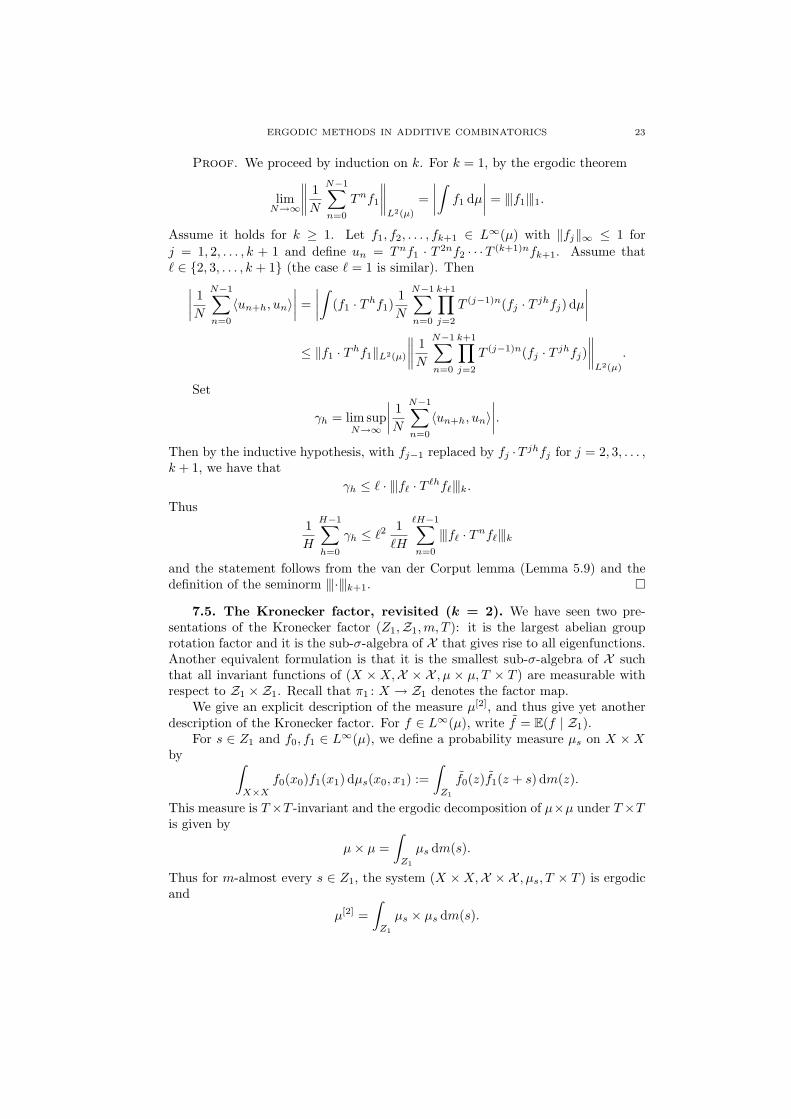
Proof. We proceed by induction on k. For k = 1, by the ergodic theorem

limN→∞

∥∥∥∥1N

N−1∑n=0

Tnf1

∥∥∥∥L2(µ)

=∣∣∣∣∫

f1 dµ

∣∣∣∣ = |‖f1‖|1.

Assume it holds for k ≥ 1. Let f1, f2, . . . , fk+1 ∈ L∞(µ) with ‖fj‖∞ ≤ 1 forj = 1, 2, . . . , k + 1 and define un = Tnf1 · T 2nf2 · · ·T (k+1)nfk+1. Assume that` ∈ {2, 3, . . . , k + 1} (the case ` = 1 is similar). Then

∣∣∣∣1N

N−1∑n=0

〈un+h, un〉∣∣∣∣ =

∣∣∣∣∫

(f1 · Thf1)1N

N−1∑n=0

k+1∏

j=2

T (j−1)n(fj · T jhfj) dµ

∣∣∣∣

≤ ‖f1 · Thf1‖L2(µ)

∥∥∥∥1N

N−1∑n=0

k+1∏

j=2

T (j−1)n(fj · T jhfj)∥∥∥∥

L2(µ)

.

Set

γh = lim supN→∞

∣∣∣∣1N

N−1∑n=0

〈un+h, un〉∣∣∣∣.

Then by the inductive hypothesis, with fj−1 replaced by fj ·T jhfj for j = 2, 3, . . . ,k + 1, we have that

γh ≤ ` · |‖f` · T `hf`‖|k.

Thus1H

H−1∑

h=0

γh ≤ `21

`H

`H−1∑n=0

|‖f` · Tnf`‖|k

and the statement follows from the van der Corput lemma (Lemma 5.9) and thedefinition of the seminorm |‖·‖|k+1. ¤

7.5. The Kronecker factor, revisited (k = 2). We have seen two pre-sentations of the Kronecker factor (Z1,Z1,m, T ): it is the largest abelian grouprotation factor and it is the sub-σ-algebra of X that gives rise to all eigenfunctions.Another equivalent formulation is that it is the smallest sub-σ-algebra of X suchthat all invariant functions of (X ×X,X × X , µ × µ, T × T ) are measurable withrespect to Z1 ×Z1. Recall that π1 : X → Z1 denotes the factor map.

We give an explicit description of the measure µ[2], and thus give yet anotherdescription of the Kronecker factor. For f ∈ L∞(µ), write f = E(f | Z1).

For s ∈ Z1 and f0, f1 ∈ L∞(µ), we define a probability measure µs on X ×Xby ∫

X×X

f0(x0)f1(x1) dµs(x0, x1) :=∫

Z1

f0(z)f1(z + s) dm(z).

This measure is T×T -invariant and the ergodic decomposition of µ×µ under T×Tis given by

µ× µ =∫

Z1

µs dm(s).

Thus for m-almost every s ∈ Z1, the system (X ×X,X × X , µs, T × T ) is ergodicand

µ[2] =∫

Z1

µs × µs dm(s).

24 B. KRA

More generally, if fε, ε ∈ {0, 1}2, are measurable functions on X, then∫

X[2]f00 ⊗ f01 ⊗ f10 ⊗ f11 dµ[2]

=∫

Z31

f00(z) · f01(z + s) · f10(z + t) · f11(z + s + t) dm(z) dm(s) dm(t).

It follows immediately that:

|‖f‖|42 :=∫

f ⊗ f ⊗ f ⊗ f dµ[2]

=∫

Z31

f(z) · f(z + s) · f(z + t) · f(z + s + t) dm(z) dm(s) dm(t).

As a corollary, |‖f‖|2 is the `4-norm of the Fourier Transform of f and thefactor Z1, defined by |‖f‖|2 = 0 if and only if E(f | Z1) = 0 for f ∈ L∞(µ), is theKronecker factor of (X,X , µ, T ).

7.6. Factors for all k ≥ 1. Using these seminorms, we define factors Zk =Zk(X) for k ≥ 1 of X that generalize the relation between the Kronecker factorZ1 and the second seminorm |‖·‖|2. We define Zk as follows: for f ∈ L∞(µ),E(f | Zk) = 0 if and only if |‖f‖|k+1 = 0. We let Zk denote the associated factor.That this does define a factor needs proof and to further explain this and thedefinition, we start by describing some geometric properties of the measures µ[k].

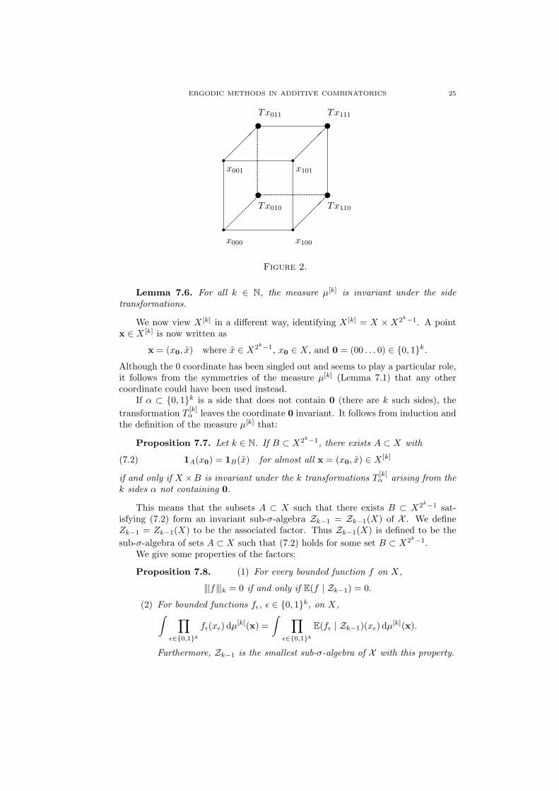
Indexing X [k] by the coordinates {0, 1}k of the Euclidean cube, it is naturalto use geometric terms like side, edge, vertex for subsets of {0, 1}k. For example,Figure 1 illustrates the point x ∈ X [3] with the side α = {010, 011, 110, 111}:

Let α ⊂ {0, 1}k be a side. The side transformation T[k]α of X [k] is defined by:

(T [k]

α x)ε

=

{Txε if ε ∈ α;xε otherwise.

We can represent the transformation Tα associated to the side {010, 011, 110, 111}by Figure 2.

Since permutations of coordinates leave the measure µ[k] invariant and acttransitively on the sides, we have:

u u

u

rr

r r

u

¡¡

¡¡

¡¡

¡¡

¡¡

¡¡

..........

..........

.....................................................................................x011 x111

x110

x101x001

x000 x100

x010

Figure 1.

ERGODIC METHODS IN ADDITIVE COMBINATORICS 25

u u

u

rr

r r

u

¡¡

¡¡

¡¡

¡¡

¡¡

¡¡

..........

..........

.....................................................................................Tx011 Tx111

Tx110

x101x001

x000 x100

Tx010

Figure 2.

Lemma 7.6. For all k ∈ N, the measure µ[k] is invariant under the sidetransformations.

We now view X [k] in a different way, identifying X [k] = X ×X2k−1. A pointx ∈ X [k] is now written as

x = (x0, x) where x ∈ X2k−1, x0 ∈ X, and 0 = (00 . . . 0) ∈ {0, 1}k.

Although the 0 coordinate has been singled out and seems to play a particular role,it follows from the symmetries of the measure µ[k] (Lemma 7.1) that any othercoordinate could have been used instead.

If α ⊂ {0, 1}k is a side that does not contain 0 (there are k such sides), thetransformation T

[k]α leaves the coordinate 0 invariant. It follows from induction and

the definition of the measure µ[k] that:

Proposition 7.7. Let k ∈ N. If B ⊂ X2k−1, there exists A ⊂ X with

(7.2) 1A(x0) = 1B(x) for almost all x = (x0, x) ∈ X [k]

if and only if X ×B is invariant under the k transformations T[k]α arising from the

k sides α not containing 0.

This means that the subsets A ⊂ X such that there exists B ⊂ X2k−1 sat-isfying (7.2) form an invariant sub-σ-algebra Zk−1 = Zk−1(X) of X . We defineZk−1 = Zk−1(X) to be the associated factor. Thus Zk−1(X) is defined to be thesub-σ-algebra of sets A ⊂ X such that (7.2) holds for some set B ⊂ X2k−1.

We give some properties of the factors:

Proposition 7.8. (1) For every bounded function f on X,

|‖f‖|k = 0 if and only if E(f | Zk−1) = 0.

(2) For bounded functions fε, ε ∈ {0, 1}k, on X,∫ ∏

ε∈{0,1}k

fε(xε) dµ[k](x) =∫ ∏

ε∈{0,1}k

E(fε | Zk−1)(xε) dµ[k](x).

Furthermore, Zk−1 is the smallest sub-σ-algebra of X with this property.

26 B. KRA

(3) The invariant sets of (X [k],X [k], µ[k], T [k]) are measurable with respectto Z [k]

k . Furthermore, Zk is the smallest sub-σ-algebra of X with thisproperty.

The proof of this proposition relies on showing a similar formula to that used(in (7.1)) to define the measures µ[k], but with respect to the new identificationseparating the 0 coordinate from the 2k − 1 others. Namely, for bounded functionsf on X and F on X2k−1,∫

X[k]f(x0) · F (x) dµ[k](x) =

∫

X[k−1]E(f | Zk−1) · E(F | Zk−1) dµ[k−1].

The given properties then follow using induction and the symmetries of the mea-sures.

We have already seen that Z0 is the trivial factor and Z1 is the Kroneckerfactor. More generally, the sequence of factors is increasing:

Z0 ← Z1 ← · · · ← Zk ← Zk+1 ← · · · ← X.

If X is weak mixing, then Zk(X) is the trivial factor for every k.An immediate consequence of Lemma 7.5 and the definition of the factors is

that the factor Zk−1 is characteristic for the average along arithmetic progressions:

Proposition 7.9. For all k ≥ 1, the factor Zk−1 is characteristic for theconvergence of the averages

1N

N−1∑n=0

Tnf1 · T 2nf2 · · · · · T knfk.

This means that in order to understand the long term behavior of the multipleaverage along a k-term arithmetic progression, it suffices to assume that the spaceitself is Zk. In particular, once we show that the factor Zk has some useful structure(and this is the content of the Structure Theorem of [34], Theorem 8.1, discussedin Section 8), we are able to prove the existence of the limit of the average alongarithmetic progressions. Proposition 7.9 would be meaningless if we were not ableto explicitly describe the structure of Zk in some way other than the abstractdefinition already given, and then use that description to prove convergence.

8. Structure theorem

8.1. Systems of order k. For k ≥ 0, an ergodic system X is said to be oforder k if Zk(X) = X. This means that |‖·‖|k+1 is a norm on L∞(µ).

Given an ergodic system (X,X , µ, T ), Zk(X) is a system of order k, sinceZk(Zk(X)) = Zk(X). The unique system of order zero is the trivial system, anda system of order 1 is an ergodic rotation. By definition, if a system is of order k,then it is also of order k′ for any k′ > k.

By Proposition 7.9, to show convergence of

1N

N−1∑n=0

Tnf1 · T 2nf2 · · · · · T knfk

in an arbitrary system, it suffices to assume that each function is defined on the fac-tor Zk−1. But since Zk−1(X) is a system of order k, it suffices to prove convergenceof this average for systems of order k − 1.

In this language, the Structure Theorem becomes:

ERGODIC METHODS IN ADDITIVE COMBINATORICS 27

Theorem 8.1 (Host and Kra [34]). A system of order k is the inverse limitof a sequence of k-step nilsystems.

Before turning to the proof of the Structure Theorem, we show convergence forthe average along arithmetic progressions in a nilsystem. Combining this conver-gence with Theorem 8.1 completes the proof of Theorem 3.1.

8.2. Convergence on a nilmanifold. Using general properties of nilmani-folds (see Furstenberg [15] and Parry [47]), Lesigne [46] showed for connected groupG and Leibman [44] showed in the general case, convergence in a nilsystem:

Theorem 8.2. If (X = G/Γ,G/Γ, µ, T ) is a nilsystem and f is a continuousfunction on X, then

1N

N−1∑n=0

f(Tnx)

converges for every x ∈ X.

(See also Ratner [50] and Shah [53] for related convergence results.)As a corollary, we have convergence in L2(µ) for the average along arithmetic

progressions in a nilmanifold:

Corollary 8.3. If (X = G/Γ,G/Γ, µ, T ) is a nilsystem, k ∈ N, and f1, f2, . . . ,fk ∈ L∞(µ), then

limN→∞

1N

N−1∑n=0

Tnf1 · T 2nf2 · · · · · T knfk

exists in L2(µ).

Proof. By density, we can assume that the functions are continuous. Byassumption, Gk is a nilpotent Lie group, Γk is a discrete cocompact subgroup andXk = Gk/Γk is a nilmanifold. Let

s = (t, t2, . . . , tk) ∈ Gk

and let S : Xk → Xk be the translation by s, meaning that

S = T × T 2 × · · · × T k.

We apply Theorem 8.2 to (Xk, S) with the continuous function

F (x1, x2, . . . , xk) = f1(x1)f2(x2) . . . fk(xk)

at the point y = (x, x, . . . , x) and so the averages converge everywhere. ¤

Thus Theorem 3.1 holds in a nilsystem, and we are left with proving the Struc-ture Theorem.

8.3. A group of transformations. To each ergodic system, we associate agroup of measure preserving transformations. The general approach is to show thatfor sufficiently many systems of order k, this group is a nilpotent Lie group. Thebulk of the work is to then show that this group acts transitively on the system.Thus the system can be given the structure of a nilmanifold and the StructureTheorem (Theorem 8.1) follows.

Most proofs are sketched or omitted completely, and the reader is referredto [34] for the details.

28 B. KRA

Let (X,X , µ, T ) be an ergodic system. If S : X → X and α ⊂ {0, 1}k, defineS

[k]α : X [k] → X [k] by:

(S[k]

α x)ε

=

{Sxε if ε ∈ α;xε otherwise.

Let G = G(X) be the group of transformations S : X → X such that for allk ∈ N and all sides α ⊂ {0, 1}k, the measure µ[k] is invariant under S

[k]α .

Some properties of this group are immediate. By symmetry, it suffices to con-sider one side. By definition, T ∈ G, and if ST = TS then we also have that S ∈ G.If S ∈ G and k ∈ N , then µ[k] is invariant under S[k] : X [k] → X [k]. Furthermore,S[k]E = E for every E ∈ I [k].

By induction, the invariance of the measure µ[k] under the side transformations,and commutator relations, we have:

Proposition 8.4. If X is a system of order k, then G(X) is a k-step nilpotentgroup.

8.4. Proof of the Structure Theorem. We proceed by induction. By theinductive assumption, we can assume that we are given a system (X,X , µ, T ) oforder k. We have a factor (Y,Y, ν, T ), where Y = Zk−1(X) and π : X → Y isthe factor map. Furthermore, Y is an inverse limit of a sequence of (k − 1)-stepnilsystems

Y = lim←−Yi; Yi = Gi/Γi.

We want to show that X is an inverse limit of k-step nilsystems.We have already shown that if fε, ε ∈ {0, 1}k, are bounded functions on X,

then ∫ ∏

ε∈{0,1}k

fε(xε) dµ[k](x) =∫ ∏

ε∈{0,1}k

E(fε | Y)(xε) dµ[k](x).

In particular, for f ∈ L∞(µ),

|‖f‖|k = 0 if and only if E(f | Y) = 0.

Furthermore, X does not admit a strict sub-σ-algebra Z such that all invariant setsof (X [k], µ[k], T [k]) are measurable with respect to Z [k]. Recall also that the system(X [k], µ[k], T [k]) is defined as a relatively independent joining.

In [16], Furstenberg described the invariant σ-algebra for an arbitrary relativelyindependent joining. It follows that X is an isometric extension of Y , meaning thatX = Y ×H/K where H is a compact group and K is a closed subgroup, µ = ν×m,where m is the Haar measure of H/K, and the transformation T is given by

T (y, u) = (Ty, ρ(y) · u)

for some map ρ : Y → H. (Note that we are making a slight, but standard, abuseof notation in using the same letter T to denote both the transformation in X andY .)

Lemma 8.5. For every h ∈ H, the transformation (y, u) 7→ (y, h · u) of Xbelongs to the center of G(X).

Thus H is abelian. We can substitute H/K for H, and we use additive notationfor H.

We therefore have more information: X is an abelian extension of Y , meaningthat X = Y ×H for some compact abelian group H, µ = ν ×m, where m is the

ERGODIC METHODS IN ADDITIVE COMBINATORICS 29

Haar measure of H, and the transformation T is given by T (y, u) = (Ty, u + ρ(y))for some map ρ : Y → H. We call ρ the cocycle defining the extension.

Furthermore, we show that the cocycle defining this extension has a particularform, given by a particular functional equation:

Proposition 8.6. If (X,X , µ, T ) is a system of order k and (Y,Y, ν, T ) =Zk−1(X), then X is an abelian extension of Y via a compact group H and for thecocycle ρ defining this extension, there exists a map Φ: Y [k] → H such that

(8.1)∑

ε∈{0,1}k

(−1)ε1+···+εkρ(yε) = Φ(T [k]y)− Φ(y)

for ν[k]-a.e. y ∈ Y [k].

We can make a few more assumptions on our system. Namely, by inductionwe can deduce that H is connected. Since every connected compact abelian groupH is an inverse limit of a sequence of tori, we can further reduce to the case thatH = Td.

8.5. The case k = 2 (The Conze – Lesigne equation). We maintain no-tation of the preceding section and review what this means for the case k = 2. Byassumption, we have that (Y,Y, ν, T ) is a system of order 1, meaning it is a grouprotation. The measure ν[2] is the Haar measure of the subgroup

{(y, y + s, y + t, y + s + t) : y, s, t ∈ Y

}

of Y 4. The functional equation of Proposition 8.6 is: there exists Φ: Y 3 → Td with

ρ(y)− ρ(y + s)− ρ(y + t) + ρ(y + s + t) = Φ(y + 1, s, t)− Φ(y, s, t)

It follows that for every s ∈ Y , there exists φs : Y → Td and cs ∈ Td satisfyingthe Conze – Lesigne equation (see [9]):

(CL) ρ(y)− ρ(y + s) = φs(y + 1)− φs(y) + cs.

The group G(X) associated to the system is the group of transformations ofX = Y × Td of the form

(y, h) 7→ (y + s, h + φs(y))

where s and φs satisfy (CL).

8.6. Structure theorem in general. We give a short outline of the stepsneeded to complete the proof of the Structure Theorem for k ≥ 3. We have thatY = Zk−1(X) is a system of order k − 1, X = Y × Td, T (y, h) = (Ty, h + ρ(y)),and ρ : Y → Td satisfies the functional equation (8.1). By the induction hypothesisY = lim←−Yi where each Yi = Gi/Γi is a (k − 1)-step nilsystem.

We first show that the cocycle ρ is cohomologous to a cocycle measurable withrespect to Yi for some i, meaning that the difference between the two cocycles isa coboundary. This reduces us to the case that ρ is measurable with respect tosome Yi, and so we can assume that Y = Yi for some i. Thus Y is a (k − 1)-stepnilsystem and we can assume that Y = G/Γ with G = G(Y ).

We then use the functional equation (8.1) to lift every transformation S ∈ Gto a transformation of X belonging to G(X). Starting with the case S ∈ Gk−1, wemove up the lower central series of G. Lastly we show that we obtain sufficientlymany elements of the group G(X) in this way.

30 B. KRA

8.7. Relations to the finite case. The seminorms |‖·‖|k play the same rolethat the Gowers norms play in Gowers’s proof [23] of Szemeredi’s theorem andin Green and Tao’s proof [25] that the primes contain arbitrarily long arithmeticprogressions. We let Uk denote the k-th Gowers norm. For the finite system Z/NZ,|‖f‖|k = ‖f‖Uk

. Furthermore, ‖·‖Ukis a norm, not only a seminorm. The analog of

Lemma 7.5 is that if ‖f0‖∞, ‖f1‖∞, . . . , ‖fk‖∞ ≤ 1, then there exists some constantCk > 0 such that∣∣E(

f0(x)f1(x + y) . . . fk(x + ky) | x, y ∈ Z/pZ)∣∣ ≤ Ck min

0≤j≤k‖fj‖Uk

.

Other parts of the program are not as easy to translate to the finite setting.Consider defining a factor of the system using the seminorms. If p is prime, thenZ/pZ has no nontrivial factor and so there is no factor of Z/pZ playing the role ofthe factor Zk, meaning there is no factor with

E(f | Zk) = 0 if and only if ‖f‖Uk= 0.

Instead, the corresponding results have a different flavor: if ‖f‖Ukis large in some

sense, then f has large conditional expectation on some (noninvariant) σ-algebraor it has large correlation with a function of some particular class. Although wehave a complete characterization of the seminorms |‖·‖|k (and so also of the factorsZk) in terms of nilmanifolds, there are only partial combinatorial characterizationsin this direction (see [26–28]).

9. Other patterns

9.1. Commuting transformations. Ergodic theory has been used to detectother patterns that occur in sets of positive upper density, using Furstenberg’scorrespondence principle and an appropriately chosen strengthening of Furstenbergmultiple recurrence. A first example is for commuting transformations:

Theorem 9.1 (Furstenberg and Katznelson [19]). Let (X,X , µ) be a prob-ability measure space, let k ≥ 1 be an integer, and assume that Tj : X → X arecommuting measure preserving transformations for j = 1, 2, . . . , k. Then for allA ∈ X with µ(A) > 0, there exist infinitely many n ∈ N such that

(9.1) µ(A ∩ T−n1 A ∩ T−n

2 A ∩ · · · ∩ T−nk A) > 0.

(In [20], Furstenberg and Katznelson proved a strengthening of this result,showing that one can place some restrictions on the choice of n; we do not discussthese “IP” versions of this theorem or the theorems given in the sequel.) Viacorrespondence, a multidimensional version of Szemeredi’s theorem follows: if E ⊂Zr has positive upper density and F ⊂ Zr is a finite subset, then there exist z ∈ Zr

and n ∈ N such that z + nF ⊂ E.Again, this theorem is proven by showing that the associated lim inf of the

average of the quantity in Equation (9.1) is positive. And again, it is natural toask whether the limit

limN→∞

1N

N−1∑n=0

µ(A ∩ T−n1 A ∩ · · · ∩ T−n

k A)

exists in L2(µ) for commuting maps T1, . . . , Tk. Only partial results are known. Fork = 2, Conze and Lesigne ([8, 9]) proved convergence. For k ≥ 3, the only knownresults rely on strong hypotheses of ergodicity:

ERGODIC METHODS IN ADDITIVE COMBINATORICS 31

Theorem 9.2 (Frantzikinakis and Kra [13]). Let k ∈ N and assume thatT1, T2, . . . , Tk are commuting invertible ergodic measure preserving transformationsof a measure space (X,X , µ) such that TiT

−1j is ergodic for all i, j ∈ {1, 2, . . . , k}

with i 6= j. If f1, f2, . . . , fk ∈ L∞(µ) the averages,

1N

N−1∑n=0

Tn1 f1 · Tn

2 f2 · · · · · Tnk fk

converge in L2(µ) as N →∞.

The idea is to prove an analog of Lemma 7.5 for commuting transformations,thus reducing the problem to working in a nilsystem. The factors Zk that are char-acteristic for averages along arithmetic progressions are also characteristic for theseparticular averages of commuting transformations. Without the strong hypothesesof ergodicity, this no longer holds and the general case remains open.

9.2. Averages along cubes. Another type of average is along k-dimensionalcubes, the natural objects that arise in the definition of the seminorms. For exam-ple, a 2-dimensional cube is an expression of the form:

f(x)f(Tmx)f(Tnx)f(Tm+nx).

In [4], Bergelson showed the existence in L2(µ) of

limN→∞

1N2

N−1∑n,m=0

Tnf1 · Tmf2 · Tn+mf3,

where f1, f2, f3 ∈ L∞(µ). Similarly, one can define a 3-dimensional cube:

f1(Tmx)f2(Tnx)f3(Tm+nx)f4(T px)f5(Tm+px)f6(Tn+px)f7(Tm+n+px)

and existence of the limit of the average of this expression L2(µ) for boundedfunctions f1, f2, . . . , f7 was shown in [33].

More generally, this theorem holds for cubes of 2k − 1 functions. Recalling thenotation of Section 7, we have for ε = ε1 . . . εk ∈ {0, 1}k and n = (n1, . . . , nk) ∈ Zk,

ε · n = ε1n1 + ε2n2 + · · ·+ εknk,

and 0 denotes the element 00 . . . 0 of {0, 1}k. We have:

Theorem 9.3 (Host and Kra [34]). Let (X,X , µ, T ) be a system, let k ≥ 1be an integer, and let fε, ε ∈ {0, 1}k \{0}, be 2k−1 bounded functions on X. Thenthe averages

1Nk·

∑

n∈[0,N−1]k

∏

ε∈{0,1}k

ε 6=0

T ε·nfε

converge in L2(µ) as N →∞.

The same result holds for translated averages, meaning the average for n ∈[M1, N1]× · · · × [Mk, Nk], as N1 −M1, . . . , Nk −Mk →∞.

By Furstenberg’s correspondence principle, this translates to a combinatorialstatement. A subset E ⊂ Z is syndetic if Z can be covered by finitely manytranslates of E. In other words, there exists N > 0 such that every interval of sizeN contains at least one element of E. (Thus it is natural to refer to a syndetic set

32 B. KRA

in the integers as a set with bounded gaps.) More generally, E ⊂ Zk is syndetic ifthere exists an integer N > 0 such that

E ∩ ([M1,M1 + N ]× · · · × [Mk,Mk + N ]

) 6= ∅for all M1, . . . ,Mk ∈ Z.

Restricting Theorem 9.3 to indicator f unctions, the limit of the averagesk∏

i=1

1Ni −Mi

·∑

n1∈[M1,N1],...,nk∈[Mk,Nk]

µ

( ⋂

ε∈{0,1}k

T ε·nA

)

exists and is greater than or equal to µ(A)2k

when N1 −M1, . . . , Nk −Mk → ∞.Thus for every ε > 0,{

n ∈ Zk : µ

( ⋂

ε∈{0,1}k

T ε·nA

)> µ(A)2

k − ε

}

of Zk is syndetic.By the correspondence principle, we have that if E ⊂ Zk has upper density

d∗(E) > δ > 0 and k ∈ N, then{n ∈ Zk : d∗

( ⋂

ε∈{0,1}k

(E + ε · n))≥ δ2k

}

is syndetic.

9.3. Polynomial patterns. In a different direction, one can restrict the it-erates arising in Furstenberg’s multiple recurrence. A natural choice is polynomialiterates, and the corresponding combinatorial statement is that a set of integerswith positive upper density contains elements who differ by a polynomial:

Theorem 9.4 (Sarkozy [51], Furstenberg [17]). If E ⊂ N has positive upperdensity and p : Z→ Z is a polynomial with p(0) = 0, then there exist x, y ∈ E andn ∈ N such that x− y = p(n).

As for arithmetic progressions, Furstenberg’s proof relies on the correspondenceprinciple and an averaging theorem:

Theorem 9.5 (Furstenberg [17]). Let (X,X , µ, T ) be a system, let A ∈ Xwith µ(A) > 0 and let p : Z→ Z be a polynomial with p(0) = 0. Then

lim infN→∞

1N

N−1∑n=0

µ(A ∩ T−p(n)A) > 0.

The multiple polynomial recurrence theorem, simultaneously generalizing thissingle polynomial result and Furstenberg’s multiple recurrence, was proven byBergelson and Leibman:

Theorem 9.6 (Bergelson and Leibman [6]). Let (X,X , µ, T ) be a system,let A ∈ X with µ(A) > 0, and let k ∈ N. If p1, p2, . . . , pk : Z → Z are polynomialswith pj(0) = 0 for j = 1, . . . , k, then

(9.2) lim infN→∞

1N

N−1∑n=0

µ(A ∩ T−p1(n)A ∩ · · · ∩ T−pk(n)A

)> 0.

ERGODIC METHODS IN ADDITIVE COMBINATORICS 33

By the correspondence principle, one immediately deduces a polynomial Sze-meredi theorem: if E ⊂ Z has positive upper density, then it contains arbitrarypolynomial patterns, meaning there exists n ∈ N such that

x, x + p1(n), x + p2(n), . . . , x + pk(n) ∈ E.

(More generally, Bergelson and Leibman proved a version of Theorem 9.6 for com-muting transformations, with a multidimensional polynomial Szemeredi theorem asa corollary.)

Again, it is natural to ask whether the lim inf in (9.2) is actually a limit. Afirst result in this direction was given by Furstenberg and Weiss [22], who provedconvergence in L2(µ) of

1N

N−1∑n=0

Tn2f1 · Tnf2

and1N

N−1∑n=0

Tn2f1 · Tn2+nf2

for bounded functions f1, f2.The proof of convergence for general polynomial averages uses the technology of

the seminorms, reducing to the same characteristic factors Zk that can be describedusing nilsystems, as for averages along arithmetic progressions:

Theorem 9.7 (Host and Kra [35], Leibman [45]). Let (X,X , µ, T ) be asystem, k ∈ N, and f1, f2, . . . , fk ∈ L∞(µ). Then for any polynomials p1, p2, . . . ,pk : Z→ Z, the averages

1N

N−1∑n=0

T p1(n)f1 · T p2(n)f2 · · · · · T pk(n)fk

converge in L2(µ).

Recently, Johnson [36] has shown that under strong ergodicity conditions, sim-ilar to those in Theorem 9.2, one can generalize this and prove L2(µ)-convergenceof the polynomial averages for commuting transformations:

1N

N−1∑n=0

Tp1(n)1 f1 · T p2(n)

2 f2 · · · · · T pk(n)k fk

for f1, f2, . . . , fk ∈ L∞(µ).For a totally ergodic system (meaning that Tn is ergodic for all n ∈ N), Fursten-

berg and Weiss showed a stronger result, giving an explicit and simple formula forthe limit:

1N

N−1∑n=0

Tnf1 · Tn2f2 →

∫f1 dµ ·

∫f2 dµ

in L2(µ).Bergelson [3] asked whether the same result holds for k polynomials of different

degrees, meaning that the limit of the polynomial average for a totally ergodicsystem is the product integrals. In [12], we show that the answer is yes under amore general condition. A family of polynomials p1, p2, . . . , pk : Z→ Z is rationallyindependent if the polynomials {1, p1, p2, . . . , pk} are linearly independent over therationals. We show:

34 B. KRA

Theorem 9.8 (Frantzikinakis and Kra [12]). Let (X,X , µ, T ) be a totallyergodic system, let k ≥ 1 be an integer, and assume that p1, p2 . . . , pk : Z → Z arerationally independent polynomials. If f1, f2, . . . , fk ∈ L∞(µ),

limN→∞

∥∥∥∥1N

N−1∑n=0

T p1(n)f1 · T p2(n)f2 · · · · · T pk(n)fk −k∏

i=1

∫fi dµ

∥∥∥∥L2(µ)

= 0.

As a corollary, if (X,X , µ, T ) is totally ergodic, {1, p1, . . . , pk} are rationallyindependent polynomials taking on integer values on the integers, and A0, A1, . . . ,Ak ∈ X with µ(Ai) > 0, i = 0, . . . , k, then

µ(A0 ∩ T−p1(n)A1 ∩ · · · ∩ T−pk(n)Ak) > 0

for some n ∈ N. Thus in a totally ergodic system, one can strengthen Bergelsonand Leibman’s multiple polynomial recurrence theorem, allowing the sets Ai to bedistinct, and allowing the polynomials pi to have nonzero constant term. It is notclear whether or not this has a combinatorial interpretation.

10. Strengthening Poincare recurrence

10.1. Khintchine recurrence. Poincare recurrence states that a set of pos-itive measure returns to intersect itself infinitely often. One way to strengthen thisis to ask that the set return to itself often with ‘large’ intersection. Khintchinemade this notion precise, showing that large self intersection occurs on a syndeticset:

Theorem 10.1 (Khintchine [37]). Let (X,X , µ, T ) be a system, let A ∈ Xhave µ(A) > 0, and let ε > 0. Then

{n ∈ Z : µ(A ∩ TnA) > µ(A)2 − ε}is syndetic.

It is natural to ask for a simultaneous generalization of Furstenberg multiplerecurrence and Khintchine recurrence. More precisely, if (X,X , µ, T ) is a system,A ∈ X has positive measure, k ∈ N, and ε > 0, is the set

{n ∈ Z : µ

(A ∩ TnA ∩ · · · ∩ T knA

)> µ(A)k+1 − ε

}

syndetic?Furstenberg multiple recurrence implies that there exists some constant c =

c(µ(A)) > 0 such that

{n ∈ Z : µ(A ∩ TnA ∩ · · · ∩ T knA) > c}is syndetic. But to generalize Khintchine recurrence, one needs c = µ(A)k+1. Itturns out that the answer depends on the length k of the arithmetic progression.

Theorem 10.2 (Bergelson, Host and Kra [5]). Let (X,X , µ, T ) be anergodic system and let A ∈ X . Then for every ε > 0, the sets

{n ∈ Z : µ(A ∩ TnA ∩ T 2nA) > µ(A)3 − ε}and

{n ∈ Z : µ(A ∩ TnA ∩ T 2nA ∩ T 3nA) > µ(A)4 − ε}are syndetic.

ERGODIC METHODS IN ADDITIVE COMBINATORICS 35

Furthermore, this result fails on average, meaning that the average of the lefthand side expressions is not necessarily greater than µ(A)3 − ε or µ(A)4 − ε, re-spectively.

On the other hand, based on an example of Ruzsa contained in the appendixof [5], we have:

Theorem 10.3 (Bergelson, Host and Kra [5]). There exists an ergodicsystem (X,X , µ, T ) and for all ` ∈ N there exists a set A = A(`) ∈ X with µ(A) > 0such that

µ(A ∩ TnA ∩ T 2nA ∩ T 3nA ∩ T 4nA) ≤ µ(A)`/2for every integer n 6= 0.

We now briefly outline the major ingredients in the proofs of these theorems.

10.2. Positive ergodic results. We start with the ergodic results needed toprove Theorem 10.2. Fix an integer k ≥ 1, an ergodic system (X,X , µ, T ), andA ∈ X with µ(A) > 0. The key ingredient is the study of the multicorrelationsequence

µ(A ∩ TnA ∩ T 2nA ∩ · · · ∩ T knA

).

More generally, for a real valued function f ∈ L∞(µ), we consider the multicorre-lation sequence

If (k, n) :=∫

f · Tnf · T 2nf · · · · · T knf dµ(x).

When k = 1, Herglotz’s theorem implies that the correlation sequence If (1, n)is the Fourier transform of some positive measure σ = σf on the torus T:

If (1, n) = σ(n) :=∫

Te2πint dσ(t).

Decomposing the measure σ into its continuous part σc and its discrete part σd,can write the multicorrelation sequence If (1, n) as the sum of two sequences

If (1, n) = σc(n) + σd(n).

The sequence {σc(n)} tends to 0 in density, meaning that

(10.1) limN→∞

supM∈Z

1M

M+N−1∑

n=M

|σc(n)| = 0.

Equivalently, for any ε > 0, the upper Banach density5 of the set {n ∈ Z : |σc(n)| >ε} is zero. The sequence {σd(n)} is almost periodic, meaning that there exists acompact abelian group G, a continuous real valued function φ on G, and a ∈ G

such that σd(n) = φ(an) for all n.A compact abelian group can be approximated by a compact abelian Lie group.

Thus any almost periodic sequence can be uniformly approximated by an almostperiodic sequence arising from a compact abelian Lie group.

In general, however, for higher k the answer is more complicated. We find asimilar decomposition for the multicorrelation sequences If (k, n) for k ≥ 2. Thenotion of an almost periodic sequence is replaced by that of a nilsequence: for an

5The upper Banach density d(E) of a set E ⊂ Z is defined by d(e) =limN→∞

PM∈Z(1/N)|E ∩ [M, M + N − 1]|.

36 B. KRA

integer k ≥ 2, a k-step nilmanifold X = G/Γ, a continuous real (or complex) valuedfunction φ on G, a ∈ G, and e ∈ X, the sequence {φ(an · e)} is called a basic k-stepnilsequence. A k-step nilsequence is a uniform limit of basic k-step nilsequences.

It follows that a 1-step nilsequence is the same as an almost periodic sequence.An inverse limit of compact abelian Lie groups is a compact group. However aninverse limit of k-step nilmanifolds is not, in general, the homogeneous space ofsome locally compact group, and so for higher k, the decomposition result musttake into account the uniform limits of basic nilsequences. We have:

Theorem 10.4 (Bergelson, Host and Kra [5]). Let (X,X , µ, T ) be anergodic system, f ∈ L∞(µ) and k ≥ 1 an integer. The sequence {If (k, n)} is thesum of a sequence tending to zero in density and a k-step nilsequence.

Due to the connections between the use of the seminorms in ergodic theoryand the Gowers uniformity norms in additive combinatorics, it is natural that nilse-quences also have a role to play on the combinatorial side. Recently, Green andTao (see [26–28]) have adapted the idea of a nilsequence to combinatorics, and thisplays a role in the asymptotics for the number of arithmetic progressions of length4 in the primes. Ben Green’s notes in this volume have more on this connection.

Finally, we explain how Theorem 10.4 can be used to prove Theorem 10.2. Let{an}n∈Z be a bounded sequence of real numbers. The syndetic supremum of thissequence is defined to be

sup{c ∈ R : {n ∈ Z : an > c} is syndetic}.Every nilsequence {an} is uniformly recurrent.6 In particular, if S = sup(an) andε > 0, then {n ∈ Z : an ≥ S − ε} is syndetic.

If {an} and {bn} are two sequences of real numbers such that an − bn tendsto 0 in density (in the sense of definition (10.1)), then the two sequences have thesame syndetic supremum. Therefore the syndetic supremums of the sequences

{µ(A ∩ TnA ∩ T 2nA)}and

{µ(A ∩ TnA ∩ T 2nA ∩ T 3nA)}are equal to the supremum of the associated nilsequences, and we are reduced toshowing that they are greater than or equal to µ(A)3 and µ(A)4, respectively.

10.3. Nonergodic counterexample. Ergodicity is not needed for Khint-chine’s theorem, but is essential for Theorem 10.2:

Theorem 10.5 (Bergelson, Host, and Kra [5]). There exists a (nonergodic)system (X,X , µ, T ), and for every ` ∈ N there exists A ∈ X with µ(A) > 0 suchthat

µ(A ∩ TnA ∩ T 2nA

) ≤ 12µ(A)`.

for integer n 6= 0.

Actually there exists a set A of arbitrarily small positive measure with

µ(A ∩ TnA ∩ T 2nA

) ≤ µ(A)−c log(µ(A))

for every integer n 6= 0 and for some positive universal constant c.

6A sequence {an} of real numbers is said to be uniformly recurrence if for all ε > 0 and allh ∈ N, the set {n : |an+h − an| < ε} is syndetic

ERGODIC METHODS IN ADDITIVE COMBINATORICS 37

The proof is based on Behrend’s construction of a set containing no arithmeticprogression of length 3:

Theorem 10.6 (Behrend [1]). For all L ∈ N, there exists a subset E ⊂{0, 1, . . . , L− 1} having more than L exp(−c

√log L) elements that does not contain

any nontrivial arithmetic progression of length 3.

Proof (of Theorem 10.5). Let X = T× T, with Haar measure µ = m×mand transformation T : X → X given by T (x, y) = (x, y + x).

Let E ⊂ {0, 1, . . . , L− 1}, not containing any nontrivial arithmetic progressionof length 3. Define

B =⋃

j∈E

[j

2L,

j

2L+

14L

),

which we consider as a subset of the torus and A = T×B.For every integer n 6= 0, we have Tn(x, y) = (x, y + nx) and

µ(A ∩ TnA ∩ T 2nA

)=

∫∫

T×T1B(y)1B(y + nx)1B(y + 2nx) dm(y) dm(x)

=∫∫

T×T1B(y)1B(y + x)1B(y + 2x) dm(y) dm(x).

Bounding this integral, we have that:

µ(A ∩ TnA ∩ T 2nA

)=

∫∫

T×T1B(y)1B(y + x)1B(y + 2x) dm(x) dm(y)

≤ m(B)4L

.

By Behrend’s theorem, we can choose the set E with cardinality on the orderof L exp(−c

√log L). Choosing L sufficiently large, a simple computation gives the

statement. ¤

For longer arithmetic progressions, the counterexample of Theorem 10.3 isbased on a construction of Ruzsa. When P is a nonconstant integer polynomial ofdegree ≤ 2, the subset

{P (0), P (1), P (2), P (3), P (4)

}

of Z is called a quadratic configuration of 5 terms, written QC5 for short.Any QC5 contains at least 3 distinct elements. An arithmetic progression of

length 5 is a QC5, corresponding to a polynomial of degree 1.

Theorem 10.7 (Ruzsa [5]). For all L ∈ N, there exists a subset E ⊂ {0, 1, . . . ,L−1} having more than L exp(−c

√log L) elements that does not contain any QC5.

Based on this, we show:

Theorem 10.8 (Bergelson, Host and Kra [5]). There exists an ergodicsystem (X,X , µ, T ) and, for every ` ∈ N, there exists A ∈ X with µ(A) > 0 suchthat

µ(A ∩ TnA ∩ T 2nA ∩ T 3nA ∩ T 4nA) ≤ 12µ(A)`

for every integer n 6= 0.

38 B. KRA

Once again, the proof gives the estimate µ(A)−c log(µ(A)), for some constantc > 0.

The construction again involves a simple example: T is the torus with Haarmeasure m, X = T×T, and µ = m×m. Let α ∈ T be irrational and let T : X → Xbe

T (x, y) = (x + α, y + 2x + α).

Combinatorially this example becomes: for all k ∈ N, there exists δ > 0 suchthat for infinitely many integers N , there is a subset A ⊂ {1, . . . , N} with |A| ≥ δNthat contains no more than 1

2δkN arithmetic progressions of length ≥ 5 with thesame difference.

10.4. Combinatorial consequences. Via a slight modification of the corre-spondence principle, each of these results translates to a combinatorial statement.For ε > 0 and E ⊂ Z with positive upper Banach density (see the definition inFootnote 5), consider the set

(10.2) {n ∈ Z : d(E ∩ (E + n) ∩ (E + 2n) ∩ · · · ∩ (E + kn)) ≥ d(Ek+1)− ε}.From Theorems 10.2 and 10.3, for k = 2 and for k = 3, this set is syndetic, whilefor k ≥ 4 there exists a set of integers E with positive upper Banach density suchthat the set in (10.2) is empty.

We can refine this a bit further. Recall the notation from Szemeredi’s theorem:for every δ > 0 and k ∈ N, there exists N(δ, k) such that for all N > N(δ, k), everysubset of {1, . . . , N} with at least δN elements contains an arithmetic progressionof length k.

For an arithmetic progression {a, a + s, . . . , a + (k− 1)s}, s is the difference ofthe progression. Write bxc for integer part of x. ¿From Szemeredi’s theorem, wecan deduce that every subset E of {1, . . . , N} with at least δN elements contains atleast bcN2c arithmetic progressions of length k, where c = c(k, δ) > 0 is a constant.Therefore the set E contains at least bc(k, δ)Nc progressions of length k with thesame difference.

The ergodic results of Theorem 10.2 give some improvement for k = 3 andk = 4 (see [5] for the precise statement). For k = 3, this was strengthened byGreen:

Theorem 10.9 (Green [24]). For all δ, ε > 0, there exists N0(δ, ε) such thatfor all N > N0(δ, ε) and any E ⊂ {1, . . . , N} with |E| ≥ δN , E contains at least(1− ε)δ3N arithmetic progressions of length 3 with the same difference.

On the other hand, the similar bound for longer progressions with length k ≥ 5does not hold. The proof in [5], based on an example of Rusza, does not use ergodictheory. We show that for all k ∈ N, there exists δ > 0 such that for infinitely manyN , there exists a subset E of {1, . . . , N} with |E| ≥ δN that contains no more than12δkN arithmetic progressions of length ≥ 5 with the same step.

10.5. Polynomial averages. One can ask whether similar lower bounds holdfor the polynomial averages. For independent polynomials, using the fact that thecharacteristic factor is the Kronecker factor, we can show:

Theorem 10.10 (Frantzikinakis and Kra [14]). Let k ∈ N, (X,X , µ, T ) be asystem, A ∈ X , and let p1, p2, . . . , pk : Z→ Z be rationally independent polynomials

ERGODIC METHODS IN ADDITIVE COMBINATORICS 39

with pi(0) = 0 for i = 1, 2, . . . , k. Then for every ε > 0, the set{n ∈ Z : µ(A ∩ T p1(n)A ∩ T p2(n) ∩ · · · ∩ T pk(n)A) > µ(A)k+1 − ε

}

is syndetic.

Once again, this result fails on average.Via correspondence, analogous to the results of Section 10.4, we have that for

E ⊂ Z and rationally independent polynomials p1, p2, . . . , pk : Z→ Z with pi(0) = 0for i = 1, 2, . . . , k, then for all ε > 0, the set

{n ∈ Z : d

(E ∩ (

E + p1(n)) ∩ · · · ∩ (

E + pk(n))) ≥ d(E)k+1 − ε

}

is syndetic.Moreover, in [14] we strengthen this and show that there are many configura-

tions with the same n giving the differences: if p1, p2, . . . , pk : Z→ Z are rationallyindependent polynomials with pi(0) = 0 for i = 1, 2, . . . , k, then for all δ, ε > 0,there exists N(δ, ε) such that for all N > N(δ, ε) and any subset E ⊂ {1, . . . , N}with |E| ≥ δN contains at least (1− ε)δk+1N configurations of the form

{x, x + p1(n), x + p2(n), . . . , x + pk(n)}for a fixed n ∈ N.

References

1. F. A. Behrend, On sets of integers which contain no three terms in arithmetic progression,Proc. Nat. Acad. Sci. U.S.A. 32 (1946), 331 – 332.

2. V. Bergelson, Weakly mixing PET, Ergodic Theory Dynam. Systems 7 (1987), no. 3, 337 –349.

3. , Ergodic Ramsey theory—an update, Ergodic Theory of Zd-Actions (Warwick, 1993 –1994) (M. Pollicott and K. Schmidt, eds.), London Math. Soc. Lecture Note Ser., vol. 228,Cambridge Univ. Press, Cambridge, 1996.

4. , The multifarious Poincare recurrence theorem, Descriptive Set Theory and Dynam-ical Systems (Marseille-Luminy, 1996) (M. Foreman, A. S. Kechris, A. Louveau, and B.Weiss, eds.), London Math. Soc. Lecture Note Ser., vol. 277, Cambridge Univ. Press, Cam-bridge, 2000, pp. 31 – 57.

5. V. Bergelson, Host B., and B. Kra, Multiple recurrence and nilsequences, Invent. Math. 160(2005), no. 2, 261 – 303.

6. V. Bergelson and A. Leibman, Polynomial extensions of van der Waerden’s and Szemeredi’stheorems, J. Amer. Math. Soc. 9 (1996), no. 3, 725 – 753.

7. J. Bourgain, On the maximal ergodic theorem for certain subsets of the positive integers,Israel J. Math. 61 (1988), no. 1, 39 – 72.

8. J.-P. Conze and E. Lesigne, Sur un theoreme ergodique pour des mesures diagonales, Prob-abilites, Publ. Inst. Rech. Math. Rennes, vol. 1987-1, Univ. Rennes I, Rennes, 1987, pp. 1 –31.

9. , Sur un theoreme ergodique pour des mesures diagonales, C. R. Acad. Sci. Paris Ser.I Math. 306 (1988), no. 12, 491 – 493.

10. I. P. Cornfeld, S. V. Fomin, and Ya. G. Sinaı, Ergodic theory, Grundlehren Math. Wiss.,vol. 245, Springer, New York, 1982.

11. P. Erdos and P. Turan, On some sequences of integers, J. London Math. Soc. 11 (1936),261 – 264.

12. N. Frantzikinakis and B. Kra, Polynomial averages converge to the product of the integrals,Israel J. Math. 148 (2005), 267 – 276.

13. , Convergence of multiple ergodic averages for some commuting transformations, Er-godic Theory Dynam. Systems 25 (2005), no. 3, 799 – 809.

14. , Ergodic averages for independent polynomials and applications, J. London Math. Soc.(2) 74 (2006), no. 1, 131 – 142.

40 B. KRA

15. H. Furstenberg, Strict ergodicity and transformations of the torus, Amer. J. Math. 83 (1961),573 – 601.

16. , Ergodic behavior of diagonal measures and a theorem of Szemeredi on arithmeticprogressions, J. Analyse Math. 31 (1977), 204 – 256.

17. , Recurrence in ergodic theory and combinatorial number theory, M. B. Porter Lectures,Princeton Univ. Press, Princeton, NJ, 1981.

18. , Nonconventional ergodic averages, The legacy of John von Neumann (Hempstead,NY, 1988), Proc. Sympos. Pure Math., vol. 50, Amer. Math. Soc., Providence, RI, 1990,pp. 43 – 56.

19. H. Furstenberg and Y. Katznelson, An ergodic Szemeredi theorem for commuting transfor-mation, J. Analyse Math. 34 (1978), 275 – 291.

20. , An ergodic Szemeredi theorem for IP-systems and combinatorial theory, J. AnalyseMath. 45 (1985), 117 – 268.

21. H. Furstenberg, Y. Katznelson, and D. Ornstein, The ergodic theoretical proof of Szemeredi’stheorem, Bull. Amer. Math. Soc. (N.S.) 7 (1982), no. 3, 527 – 552.

22. H. Furstenberg and B. Weiss, A mean ergodic theorem for (1/N)PN

n=1 f(T nx)g(T n2x), Con-

vergence in Ergodic Theory and Probability (Columbus, OH, 1993), Ohio State Univ. Math.Res. Inst. Publ., vol. 5, de Gruyter, Berlin, 1996, pp. 193 – 227.

23. W. T. Gowers, A new proof of Szemeredi’s theorem, Geom. Funct. Anal. 11 (2001), no. 3,465 – 588.

24. B. J. Green, A Szemeredi-type regularity lemma in abelian groups, with applications, Geom.Funct. Anal. 15 (2005), no. 2, 340 – 376.

25. B. J. Green and T. C. Tao, The primes contain arbitrarily long arithmetic progressions, Ann.of Math. (2), to appear.

26. , An inverse theorem for the Gowers U3-norm, with applications, Proc. Edinb. Math.Soc. (2), to appear.

27. , Quadratic uniformity of the Mobius function, preprint.28. , Linear equations in primes, preprint.29. P. Hall, A contribution to the theory of groups of prime-power order, Proc. London Math.

Soc. 36 (1933), 29 – 95.30. P. R. Halmos and J. von Neumann, Operator methods in classical mechanics. II, Ann. of

Math. (2) 43 (1942), 332 – 350.31. B. Host, Convergence of multiple ergodic averages, School on Information and Randomness

(Santiago, 2004), to appear.32. B. Host and B. Kra, Convergence of Conze – Lesigne averages, Ergodic Theory Dynam. Sys-

tems 21 (2001), no. 2, 493 – 509.33. , Averaging along cubes, Modern Dynamical Systems and Applications, Cambridge

Univ. Press, Cambridge, 2004, pp. 123 – 144.34. , Nonconventional ergodic averages and nilmanifolds, Ann. of Math. (2) 161 (2005),

no. 1, 397 – 488.35. , Convergence of polynomial ergodic averages, Israel J. Math. 149 (2005), 1 – 19.36. M. Johnson, Convergence of polynomial ergodic averages of several variables for some com-

muting transformations, preprint.37. A. Y. Khintchine, Eine Verscharfung des Poincareschen “Wiederkehrsatzes”, Compositio

Math. 1 (1934), 177 – 179.38. B. O. Koopman and J. von Neumann, Dynamical systems of continuous spectra, Proc. Nat.

Acad. Sci. U.S.A. 18 (1932), 255 – 263.39. B. Kra, The Green –Tao theorem on arithmetic progressions in the primes: an ergodic of

view, Bull. Amer. Math. Soc. (N.S.) 43 (2006), no. 1, 3 – 23.40. , From combinatorics to ergodic theory and back again, Proceddings of the Interna-

tional Congress of Mathematicians, Vol. 3 (Madrid, 2006).41. L. Kuipers and N. Niederreiter, Uniform distribution of sequences, Pure Appl. Math., John

Wiley & Sons, New York, 1974.42. M. Lazard, Sur certaines suites d’elements dans les groupes libres et leurs extensions, C. R.

Acad. Sci. Paris 236 (1953), 36 – 38.43. A. Leibman, Polynomial sequences in groups, J. Algebra 201 (1998), no. 1, 189 – 206.44. , Pointwise convergence of ergodic averages for polynomial sequences of translations

on a nilmanifold, Ergodic Theory Dynam. Systems 25 (2005), no. 1, 201 – 213.

ERGODIC METHODS IN ADDITIVE COMBINATORICS 41

45. , Convergence of multiple ergodic averages along polynomials of several variables, IsraelJ. Math. 146 (2005), 303 – 316.

46. E. Lesigne, Sur une nil-variete, les parties minimales associeee a une translation sont unique-ment ergodiques, Ergodic Theory Dynam. Systems 11 (1991), no. 2, 379 – 391.

47. W. Parry, Ergodic properties of affine transformations and flows on nilmanifolds, Amer. J.Math. 91 (1969), 757 – 771.

48. J. Petresco, Sur les commutateurs, Math. Z. 61 (1954), 348 – 356.49. H. Poincare, Les methodes nouvelles de la mecanique celeste. I, Gathiers-Villars, Paris, 1892;

II, 1893; III, 1899.50. M. Ratner, On Raghunathan’s measure conjecture, Ann. of Math. (2) 134 (1991), no. 3, 545 –

607.51. A. Sarkozy, On difference sets of sequences of integers. I, Acta Math. Acad. Sci. Hungar. 31

(1978), no. 1-2, 125 – 149.52. , On difference sets of sequences of integers. III, Acta Math. Acad. Sci. Hungar. 31

(1978), no. 3-4, 355 – 386.53. N. Shah, Invariant measures and orbit closures on homogeneous spaces for actions of sub-

groups, Lie Groups and Ergodic Theory (Mumbai, 996), Tata Inst. Fund. Res., Bombay, 1998.54. E. Szemeredi, On sets of integers containing no k elements in arithmetic progression, Acta

Arith. 27 (1975), 199 – 245.55. J. von Neumann, Proof of the quasi-ergodic hypothesis, Proc. Nat. Acad. Sci. U.S.A. 18 (1932),

70 – 82.56. T. Ziegler, A non-conventional ergodic theorem for a nilsystem, Ergodic Theory Dynam.

Systems 25 (2005), no. 4, 1357 – 1370.57. , Universal characteristic factors and Furstenberg averages, J. Amer. Math. Soc. 20

(2007), no. 1, 53 – 97.

Department of Mathematics, Northwestern University, 2033 Sheridan Road, Ev-anston, IL 60208-2730, USA

E-mail address: kra@math.northwestern.edu