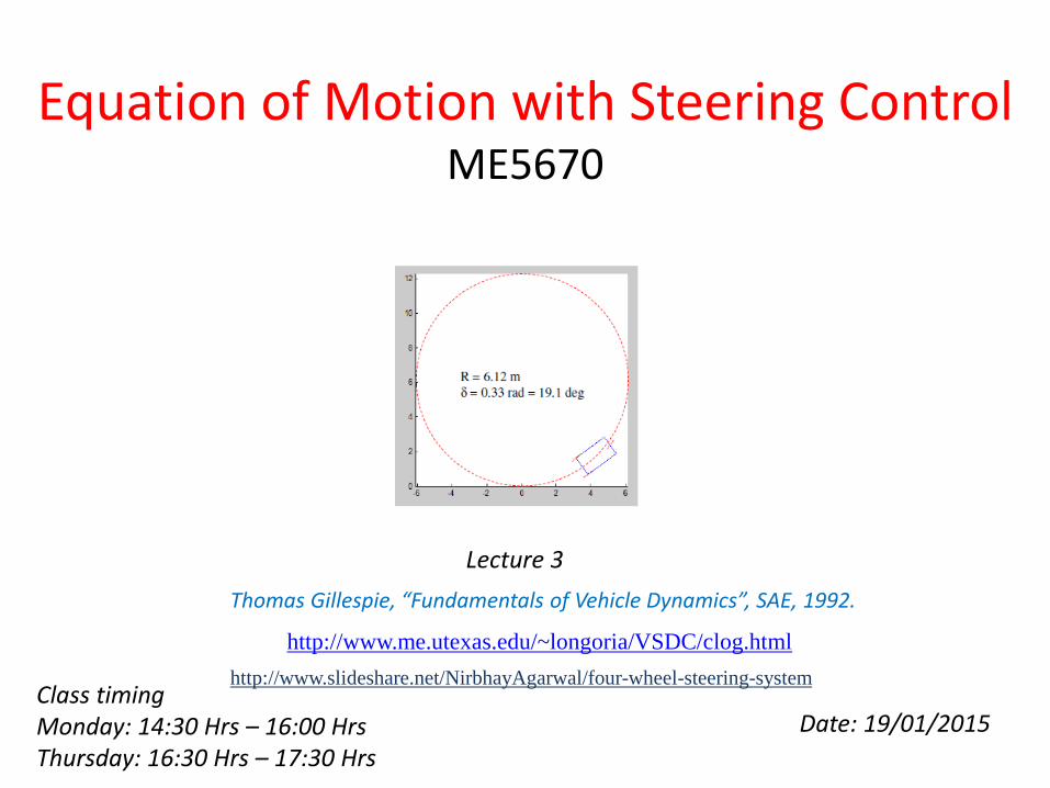
Equation of Motion with Steering Control ME5670

Date: 19/01/2015

Lecture 3

http://www.me.utexas.edu/~longoria/VSDC/clog.html

Thomas Gillespie, “Fundamentals of Vehicle Dynamics”, SAE, 1992.

http://www.slideshare.net/NirbhayAgarwal/four-wheel-steering-system Class timing Monday: 14:30 Hrs – 16:00 Hrs Thursday: 16:30 Hrs – 17:30 Hrs

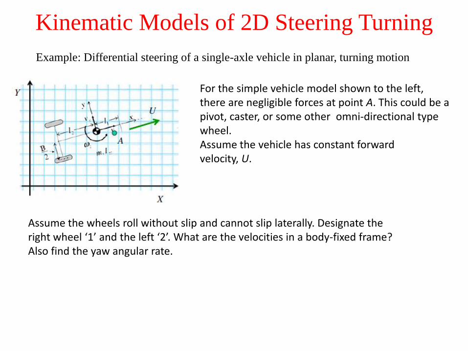
Kinematic Models of 2D Steering Turning

Example: Differential steering of a single-axle vehicle in planar, turning motion

For the simple vehicle model shown to the left, there are negligible forces at point A. This could be a pivot, caster, or some other omni-directional type wheel. Assume the vehicle has constant forward velocity, U.

Assume the wheels roll without slip and cannot slip laterally. Designate the right wheel ‘1’ and the left ‘2’. What are the velocities in a body-fixed frame? Also find the yaw angular rate.

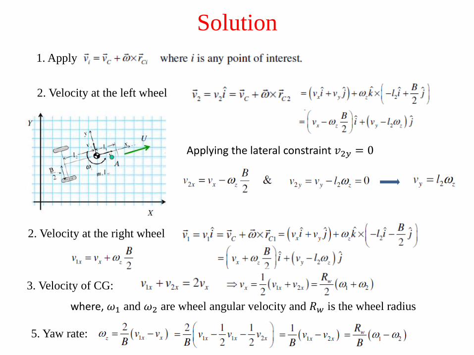
Solution

1. Apply

2. Velocity at the left wheel

Applying the lateral constraint 𝑣2𝑦 = 0

2. Velocity at the right wheel

3. Velocity of CG:

where, 𝜔1 and 𝜔2 are wheel angular velocity and 𝑅𝑤 is the wheel radius

5. Yaw rate:

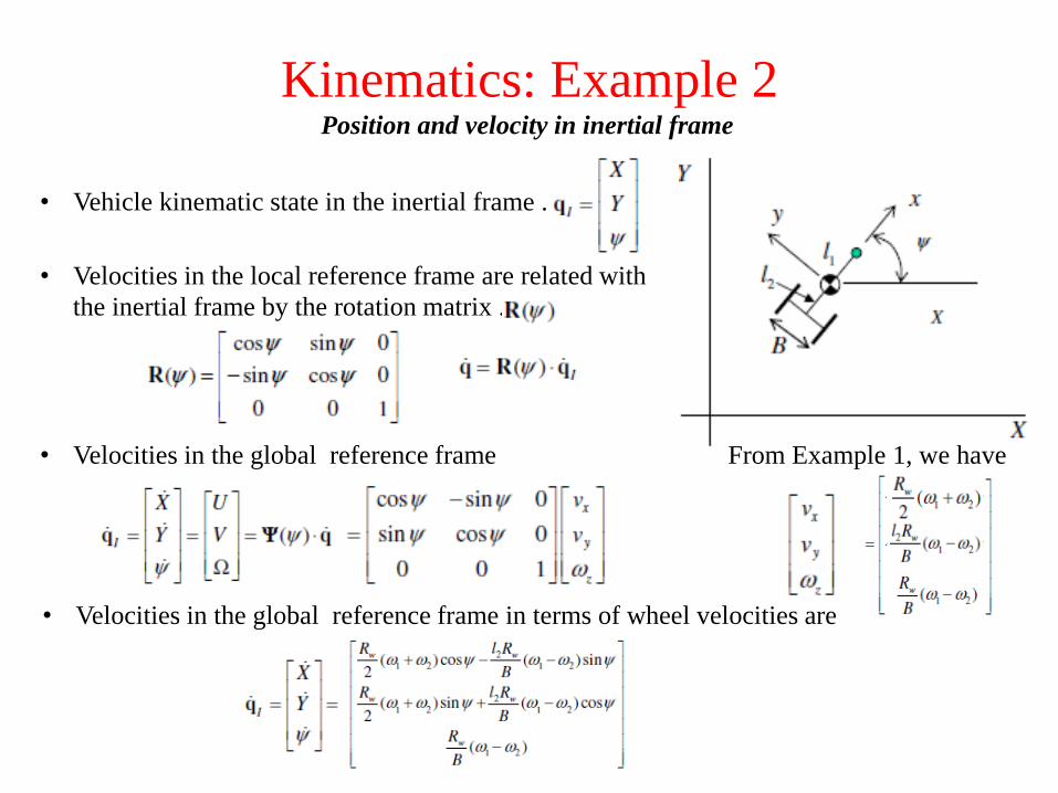
Kinematics: Example 2 Position and velocity in inertial frame

• Vehicle kinematic state in the inertial frame .

• Velocities in the local reference frame are related with

the inertial frame by the rotation matrix .

• Velocities in the global reference frame From Example 1, we have

• Velocities in the global reference frame in terms of wheel velocities are

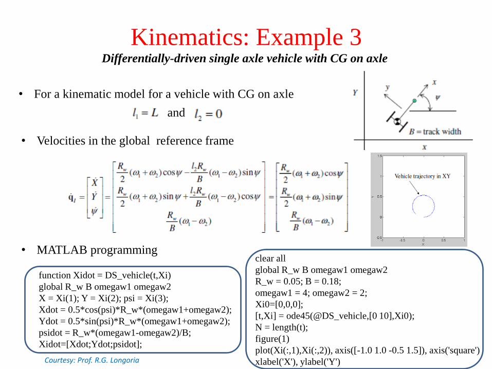
Kinematics: Example 3 Differentially-driven single axle vehicle with CG on axle

• For a kinematic model for a vehicle with CG on axle

• Velocities in the global reference frame

and

• MATLAB programming

function Xidot = DS_vehicle(t,Xi)

global R_w B omegaw1 omegaw2

X = Xi(1); Y = Xi(2); psi = Xi(3);

Xdot = 0.5*cos(psi)*R_w*(omegaw1+omegaw2);

Ydot = 0.5*sin(psi)*R_w*(omegaw1+omegaw2);

psidot = R_w*(omegaw1-omegaw2)/B;

Xidot=[Xdot;Ydot;psidot];

clear all

global R_w B omegaw1 omegaw2

R_w = 0.05; B = 0.18;

omegaw1 = 4; omegaw2 = 2;

Xi0=[0,0,0];

[t,Xi] = ode45(@DS_vehicle,[0 10],Xi0);

N = length(t);

figure(1)

plot(Xi(:,1),Xi(:,2)), axis([-1.0 1.0 -0.5 1.5]), axis('square')

xlabel('X'), ylabel('Y') Courtesy: Prof. R.G. Longoria

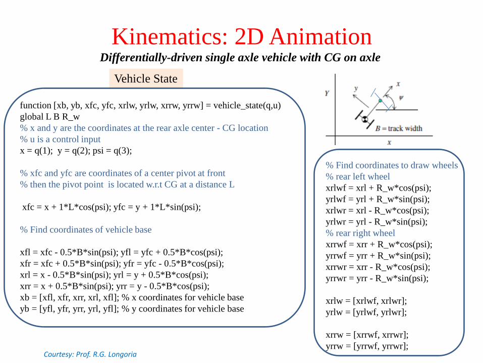
Kinematics: 2D Animation Differentially-driven single axle vehicle with CG on axle

Vehicle State

function [xb, yb, xfc, yfc, xrlw, yrlw, xrrw, yrrw] = vehicle_state(q,u)

global L B R_w

% x and y are the coordinates at the rear axle center - CG location

% u is a control input

x = q(1); y = q(2); psi = q(3);

% xfc and yfc are coordinates of a center pivot at front

% then the pivot point is located w.r.t CG at a distance L

xfc = x + 1*L*cos(psi); yfc = y + 1*L*sin(psi);

% Find coordinates of vehicle base

xfl = xfc - 0.5*B*sin(psi); yfl = yfc + 0.5*B*cos(psi);

xfr = xfc + 0.5*B*sin(psi); yfr = yfc - 0.5*B*cos(psi);

xrl = x - 0.5*B*sin(psi); yrl = y + 0.5*B*cos(psi);

xrr = x + 0.5*B*sin(psi); yrr = y - 0.5*B*cos(psi);

xb = [xfl, xfr, xrr, xrl, xfl]; % x coordinates for vehicle base

yb = [yfl, yfr, yrr, yrl, yfl]; % y coordinates for vehicle base

% Find coordinates to draw wheels

% rear left wheel

xrlwf = xrl + R_w*cos(psi);

yrlwf = yrl + R_w*sin(psi);

xrlwr = xrl - R_w*cos(psi);

yrlwr = yrl - R_w*sin(psi);

% rear right wheel

xrrwf = xrr + R_w*cos(psi);

yrrwf = yrr + R_w*sin(psi);

xrrwr = xrr - R_w*cos(psi);

yrrwr = yrr - R_w*sin(psi);

xrlw = [xrlwf, xrlwr];

yrlw = [yrlwf, yrlwr];

xrrw = [xrrwf, xrrwr];

yrrw = [yrrwf, yrrwr]; Courtesy: Prof. R.G. Longoria

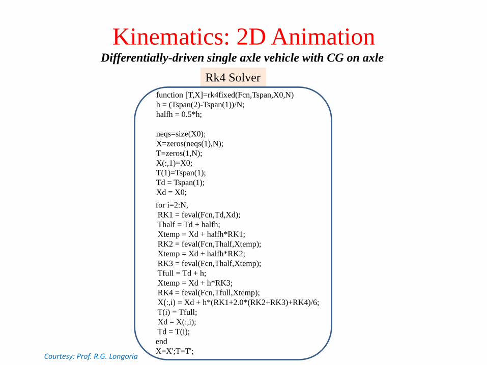
Kinematics: 2D Animation Differentially-driven single axle vehicle with CG on axle

Rk4 Solver

function [T,X]=rk4fixed(Fcn,Tspan,X0,N)

h = (Tspan(2)-Tspan(1))/N;

halfh = 0.5*h;

neqs=size(X0);

X=zeros(neqs(1),N);

T=zeros(1,N);

X(:,1)=X0;

T(1)=Tspan(1);

Td = Tspan(1);

Xd = X0;

for i=2:N,

RK1 = feval(Fcn,Td,Xd);

Thalf = Td + halfh;

Xtemp = Xd + halfh*RK1;

RK2 = feval(Fcn,Thalf,Xtemp);

Xtemp = Xd + halfh*RK2;

RK3 = feval(Fcn,Thalf,Xtemp);

Tfull = Td + h;

Xtemp = Xd + h*RK3;

RK4 = feval(Fcn,Tfull,Xtemp);

X(:,i) = Xd + h*(RK1+2.0*(RK2+RK3)+RK4)/6;

T(i) = Tfull;

Xd = X(:,i);

Td = T(i);

end

X=X';T=T'; Courtesy: Prof. R.G. Longoria

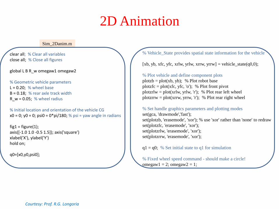
clear all; % Clear all variables close all; % Close all figures global L B R_w omegaw1 omegaw2 % Geometric vehicle parameters L = 0.20; % wheel base B = 0.18; % rear axle track width R_w = 0.05; % wheel radius % Initial location and orientation of the vehicle CG x0 = 0; y0 = 0; psi0 = 0*pi/180; % psi = yaw angle in radians fig1 = figure(1); axis([-1.0 1.0 -0.5 1.5]); axis('square') xlabel('X'), ylabel('Y') hold on; q0=[x0,y0,psi0];

% Vehicle_State provides spatial state information for the vehicle

[xb, yb, xfc, yfc, xrlw, yrlw, xrrw, yrrw] = vehicle_state(q0,0);

% Plot vehicle and define component plots

plotzb = plot(xb, yb); % Plot robot base

plotzfc = plot(xfc, yfc, 'o'); % Plot front pivot

plotzrlw = plot(xrlw, yrlw, 'r'); % Plot rear left wheel

plotzrrw = plot(xrrw, yrrw, 'r'); % Plot rear right wheel

% Set handle graphics parameters and plotting modes

set(gca, 'drawmode','fast');

set(plotzb, 'erasemode', 'xor'); % use 'xor' rather than 'none' to redraw

set(plotzfc, 'erasemode', 'xor');

set(plotzrlw, 'erasemode', 'xor');

set(plotzrrw, 'erasemode', 'xor');

q1 = q0; % Set initial state to q1 for simulation

% Fixed wheel speed command - should make a circle!

omegaw1 = 2; omegaw2 = 1;

Sim_2Danim.m

2D Animation

Courtesy: Prof. R.G. Longoria

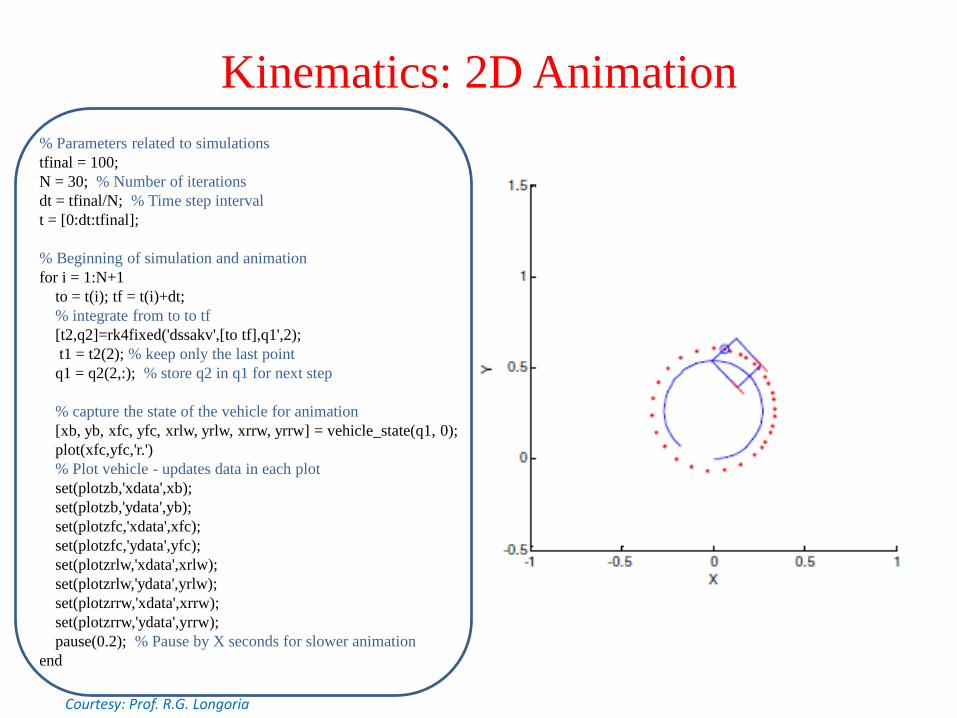
% Parameters related to simulations

tfinal = 100;

N = 30; % Number of iterations

dt = tfinal/N; % Time step interval

t = [0:dt:tfinal];

% Beginning of simulation and animation

for i = 1:N+1

to = t(i); tf = t(i)+dt;

% integrate from to to tf

[t2,q2]=rk4fixed('dssakv',[to tf],q1',2);

t1 = t2(2); % keep only the last point

q1 = q2(2,:); % store q2 in q1 for next step

% capture the state of the vehicle for animation

[xb, yb, xfc, yfc, xrlw, yrlw, xrrw, yrrw] = vehicle_state(q1, 0);

plot(xfc,yfc,'r.')

% Plot vehicle - updates data in each plot

set(plotzb,'xdata',xb);

set(plotzb,'ydata',yb);

set(plotzfc,'xdata',xfc);

set(plotzfc,'ydata',yfc);

set(plotzrlw,'xdata',xrlw);

set(plotzrlw,'ydata',yrlw);

set(plotzrrw,'xdata',xrrw);

set(plotzrrw,'ydata',yrrw);

pause(0.2); % Pause by X seconds for slower animation

end

Kinematics: 2D Animation

Courtesy: Prof. R.G. Longoria

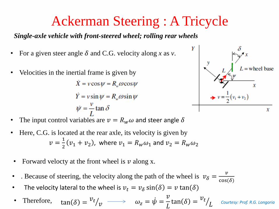
Ackerman Steering : A Tricycle Single-axle vehicle with front-steered wheel; rolling rear wheels

• For a given steer angle 𝛿 and C.G. velocity along x as v.

• Velocities in the inertial frame is given by

• The input control variables are 𝑣 = 𝑅𝑤𝜔 and steer angle 𝛿

• Therefore,

• Here, C.G. is located at the rear axle, its velocity is given by

𝑣 =1

2𝑣1 + 𝑣2 , where 𝑣1 = 𝑅𝑤𝜔1 and 𝑣2 = 𝑅𝑤𝜔2

• Forward velocty at the front wheel is 𝑣 along x.

• . Because of steering, the velocity along the path of the wheel is 𝑣𝛿 =𝑣

cos (𝛿)

• The velocity lateral to the wheel is 𝑣𝑡 = 𝑣𝛿 sin 𝛿 = 𝑣 tan (𝛿)

tan 𝛿 =𝑣𝑡

𝑣 𝜔𝑧 = 𝜓 =𝑣

𝐿tan 𝛿 =

𝑣𝑡𝐿 Courtesy: Prof. R.G. Longoria

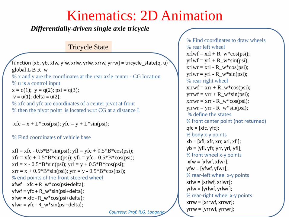
Kinematics: 2D Animation Differentially-driven single axle tricycle

Tricycle State

function [xb, yb, xfw, yfw, xrlw, yrlw, xrrw, yrrw] = tricycle_state(q, u) global L B R_w

% x and y are the coordinates at the rear axle center - CG location

% u is a control input

x = q(1); y = q(2); psi = q(3);

v = u(1); delta = u(2); % xfc and yfc are coordinates of a center pivot at front

% then the pivot point is located w.r.t CG at a distance L

xfc = x + L*cos(psi); yfc = y + L*sin(psi);

% Find coordinates of vehicle base

xfl = xfc - 0.5*B*sin(psi); yfl = yfc + 0.5*B*cos(psi);

xfr = xfc + 0.5*B*sin(psi); yfr = yfc - 0.5*B*cos(psi);

xrl = x - 0.5*B*sin(psi); yrl = y + 0.5*B*cos(psi);

xrr = x + 0.5*B*sin(psi); yrr = y - 0.5*B*cos(psi);

% end points of the front-steered wheel xfwf = xfc + R_w*cos(psi+delta); yfwf = yfc + R_w*sin(psi+delta); xfwr = xfc - R_w*cos(psi+delta); yfwr = yfc - R_w*sin(psi+delta);

% Find coordinates to draw wheels

% rear left wheel

xrlwf = xrl + R_w*cos(psi);

yrlwf = yrl + R_w*sin(psi);

xrlwr = xrl - R_w*cos(psi);

yrlwr = yrl - R_w*sin(psi);

% rear right wheel

xrrwf = xrr + R_w*cos(psi);

yrrwf = yrr + R_w*sin(psi);

xrrwr = xrr - R_w*cos(psi);

yrrwr = yrr - R_w*sin(psi);

% define the states % front center point (not returned) qfc = [xfc, yfc]; % body x-y points xb = [xfl, xfr, xrr, xrl, xfl]; yb = [yfl, yfr, yrr, yrl, yfl]; % front wheel x-y points xfw = [xfwf, xfwr]; yfw = [yfwf, yfwr]; % rear-left wheel x-y points xrlw = [xrlwf, xrlwr]; yrlw = [yrlwf, yrlwr]; % rear-right wheel x-y points xrrw = [xrrwf, xrrwr]; yrrw = [yrrwf, yrrwr];

Courtesy: Prof. R.G. Longoria

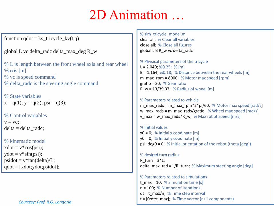
function qdot = ks_tricycle_kv(t,q)

global L vc delta_radc delta_max_deg R_w

% L is length between the front wheel axis and rear wheel

%axis [m]

% vc is speed command

% delta_radc is the steering angle command

% State variables

x = q(1); y = q(2); psi = q(3);

% Control variables

v = vc;

delta = delta_radc;

% kinematic model

xdot = v*cos(psi);

ydot = v*sin(psi);

psidot = v*tan(delta)/L;

qdot = [xdot;ydot;psidot];

% sim_tricycle_model.m clear all; % Clear all variables close all; % Close all figures global L B R_w vc delta_radc % Physical parameters of the tricycle L = 2.040; %0.25; % [m] B = 1.164; %0.18; % Distance between the rear wheels [m] m_max_rpm = 8000; % Motor max speed [rpm] gratio = 20; % Gear ratio R_w = 13/39.37; % Radius of wheel [m] % Parameters related to vehicle m_max_rads = m_max_rpm*2*pi/60; % Motor max speed [rad/s] w_max_rads = m_max_rads/gratio; % Wheel max speed [rad/s] v_max = w_max_rads*R_w; % Max robot speed [m/s] % Initial values x0 = 0; % Initial x coodinate [m] y0 = 0; % Initial y coodinate [m] psi_deg0 = 0; % Initial orientation of the robot (theta [deg]) % desired turn radius R_turn = 3*L; delta_max_rad = L/R_turn; % Maximum steering angle [deg] % Parameters related to simulations t_max = 10; % Simulation time [s] n = 100; % Number of iterations dt = t_max/n; % Time step interval t = [0:dt:t_max]; % Time vector (n+1 components)

2D Animation …

Courtesy: Prof. R.G. Longoria

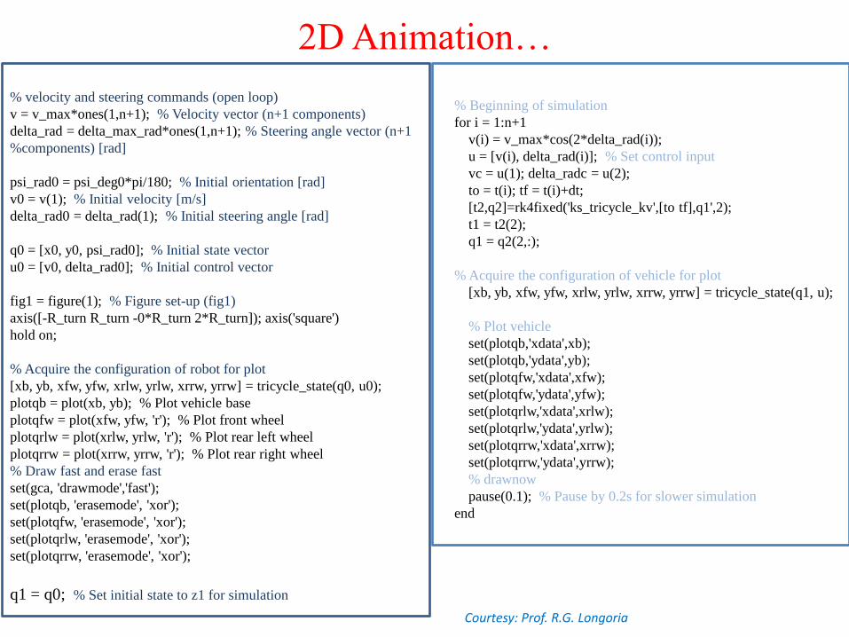
% velocity and steering commands (open loop)

v = v_max*ones(1,n+1); % Velocity vector (n+1 components)

delta_rad = delta_max_rad*ones(1,n+1); % Steering angle vector (n+1

%components) [rad]

psi_rad0 = psi_deg0*pi/180; % Initial orientation [rad]

v0 = v(1); % Initial velocity [m/s]

delta_rad0 = delta_rad(1); % Initial steering angle [rad]

q0 = [x0, y0, psi_rad0]; % Initial state vector

u0 = [v0, delta_rad0]; % Initial control vector

fig1 = figure(1); % Figure set-up (fig1)

axis([-R_turn R_turn -0*R_turn 2*R_turn]); axis('square')

hold on;

% Acquire the configuration of robot for plot

[xb, yb, xfw, yfw, xrlw, yrlw, xrrw, yrrw] = tricycle_state(q0, u0);

plotqb = plot(xb, yb); % Plot vehicle base

plotqfw = plot(xfw, yfw, 'r'); % Plot front wheel

plotqrlw = plot(xrlw, yrlw, 'r'); % Plot rear left wheel

plotqrrw = plot(xrrw, yrrw, 'r'); % Plot rear right wheel

% Draw fast and erase fast

set(gca, 'drawmode','fast');

set(plotqb, 'erasemode', 'xor');

set(plotqfw, 'erasemode', 'xor');

set(plotqrlw, 'erasemode', 'xor');

set(plotqrrw, 'erasemode', 'xor');

q1 = q0; % Set initial state to z1 for simulation

% Beginning of simulation

for i = 1:n+1

v(i) = v_max*cos(2*delta_rad(i));

u = [v(i), delta_rad(i)]; % Set control input

vc = u(1); delta_radc = u(2);

to = t(i); tf = t(i)+dt;

[t2,q2]=rk4fixed('ks_tricycle_kv',[to tf],q1',2);

t1 = t2(2);

q1 = q2(2,:);

% Acquire the configuration of vehicle for plot

[xb, yb, xfw, yfw, xrlw, yrlw, xrrw, yrrw] = tricycle_state(q1, u);

% Plot vehicle

set(plotqb,'xdata',xb);

set(plotqb,'ydata',yb);

set(plotqfw,'xdata',xfw);

set(plotqfw,'ydata',yfw);

set(plotqrlw,'xdata',xrlw);

set(plotqrlw,'ydata',yrlw);

set(plotqrrw,'xdata',xrrw);

set(plotqrrw,'ydata',yrrw);

% drawnow

pause(0.1); % Pause by 0.2s for slower simulation

end

2D Animation…

Courtesy: Prof. R.G. Longoria

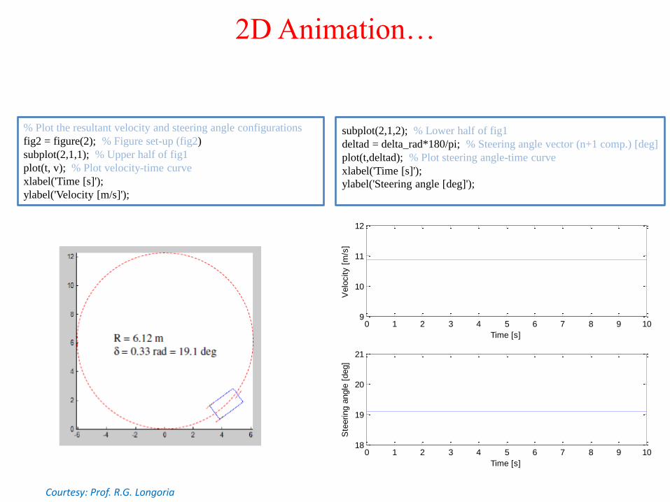
% Plot the resultant velocity and steering angle configurations

fig2 = figure(2); % Figure set-up (fig2)

subplot(2,1,1); % Upper half of fig1

plot(t, v); % Plot velocity-time curve

xlabel('Time [s]');

ylabel('Velocity [m/s]');

subplot(2,1,2); % Lower half of fig1

deltad = delta_rad*180/pi; % Steering angle vector (n+1 comp.) [deg]

plot(t,deltad); % Plot steering angle-time curve

xlabel('Time [s]');

ylabel('Steering angle [deg]');

0 1 2 3 4 5 6 7 8 9 109

10

11

12

Time [s]V

elo

city [

m/s

]

0 1 2 3 4 5 6 7 8 9 1018

19

20

21

Time [s]

Ste

ering a

ngle

[deg]

2D Animation…

Courtesy: Prof. R.G. Longoria

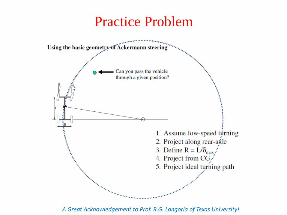
Practice Problem

A Great Acknowledgement to Prof. R.G. Longoria of Texas University!