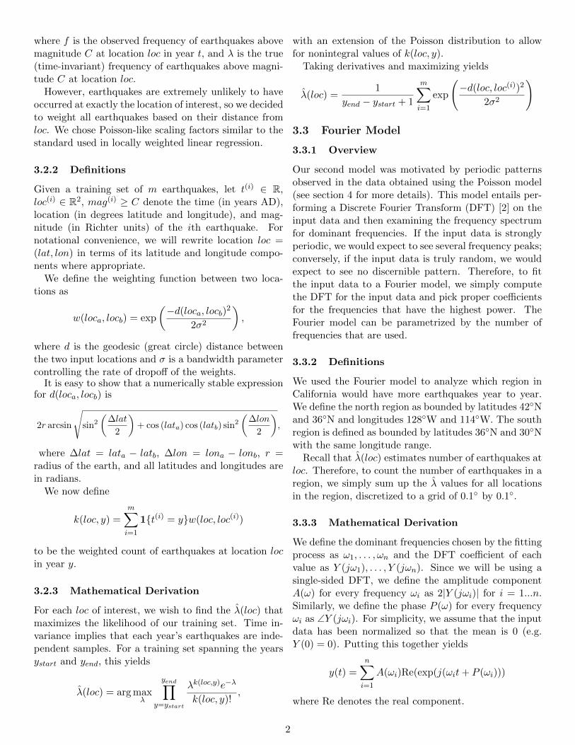
EPiC: Earthquake Prediction in California

Caroline Suen David Lo Frank Li

December 10, 2010

1 Introduction

Earthquake prediction has long been the holy grail forseismologists around the world. The various factorsaffecting earthquakes are far from being understood,and there exist no known correlations between large-scale earthquake activity and periodic geological events.Nonetheless, we hope that machine learning will give usgreater insight into the patterns underlying earthquakeactivity, even if we cannot predict the time, location,and strength of the earthquakes accurately.

2 Background

With the exception of a brief period in the 1970s, earth-quake prediction was generally considered to be infea-sible by seismologists. Then, in 1975, Chinese officialsordered the evacuation of Haicheng one day before amagnitude 7.3 earthquake struck [15]. This led to aflurry of optimism toward earthquake prediction [9, 11],which was subsequently checked by the failed predic-tion of the magnitude 7.8 Tangshan earthquake of 1976.Another failure occurred in Parkfield, California in theearly 1980s. Up to then, magnitude 6.0 earthquakes hadoccurred at fairly regular 22-year intervals. This led re-searchers to predict that an earthquake would strike by1993; no such earthquake arrived until 2004. To thisday, the Haicheng earthquake remains the only success-ful earthquake prediction in history. Critically review-ing earlier reports of successful earthquake predictions,an international panel of geologists famously concludedin 1997 that “earthquakes cannot be predicted” [4].

More recently, researchers in China have suggestedthat neural networks ensembles and support vector ma-chines could be used to predict the magnitudes of strongearthquakes [5, 16], but more research needs to be doneto corroborate their findings. For now the best earth-quake forecast is vague at best: the USGS predicts a 63%probability of one or more magnitude 6.7 earthquakes inthe San Francisco Bay Area between 2007 and 2036 [1].Rather than attempt to issue earthquake predictions, wehope to analyze past data for periodic patterns that mayadvance our understanding of earthquake dynamics.

3 Methodology

3.1 Data

For data quality purposes, we decided to focus on earth-quakes in California, which is heavily monitored forearthquake activity. We scraped, parsed, and removedduplicates from the following data sources:

• National Geophysical Data Center [7, 8]

• Northern California Earthquake Data Center [6]

• Southern California Earthquake Data Center [10]

Each of these data sources is freely available and con-tains magnitude, epicenter location, and time of occur-rence information for earthquakes dating back to 1930.

The data set is not well populated before 1970, and thenumber of earthquakes records increases rapidly there-after. This is partly due to advances in measurementtechnology and roughly corresponds to the NorthernCalifornia Seismic Network being brought online.

3.2 Poisson Model

3.2.1 Overview

Our initial model sought to estimate the number ofearthquakes at a particular location in the next year. Indeveloping the model we had several relevant features toconsider, including magnitude, latitude and longitude ofthe epicenter, depth of the epicenter, and starting timeof each earthquake. For our initial model, we made twosimplifications:

• time invariance: that the frequency of earth-quakes at a particular location did not change overtime

• magnitude insensitivity: that all earthquakesabove a specified magnitude threshold C were con-sidered equally

By not differentiating time and magnitude, we couldmodel the number of earthquakes per year at a speci-fied location as a Poisson distribution. That is,

f(loc, t) = f(loc) ∼ Poisson(λ(loc)),

1

where f is the observed frequency of earthquakes abovemagnitude C at location loc in year t, and λ is the true(time-invariant) frequency of earthquakes above magni-tude C at location loc.

However, earthquakes are extremely unlikely to haveoccurred at exactly the location of interest, so we decidedto weight all earthquakes based on their distance fromloc. We chose Poisson-like scaling factors similar to thestandard used in locally weighted linear regression.

3.2.2 Definitions

Given a training set of m earthquakes, let t(i) ∈ R,loc(i) ∈ R2, mag(i) ≥ C denote the time (in years AD),location (in degrees latitude and longitude), and mag-nitude (in Richter units) of the ith earthquake. Fornotational convenience, we will rewrite location loc =(lat, lon) in terms of its latitude and longitude compo-nents where appropriate.

We define the weighting function between two loca-tions as

w(loca, locb) = exp

(−d(loca, locb)

2

2σ2

),

where d is the geodesic (great circle) distance betweenthe two input locations and σ is a bandwidth parametercontrolling the rate of dropoff of the weights.

It is easy to show that a numerically stable expressionfor d(loca, locb) is

2r arcsin

√sin2

(∆lat

2

)+ cos (lata) cos (latb) sin2

(∆lon

2

),

where ∆lat = lata − latb, ∆lon = lona − lonb, r =radius of the earth, and all latitudes and longitudes arein radians.

We now define

k(loc, y) =m∑i=1

1{t(i) = y}w(loc, loc(i))

to be the weighted count of earthquakes at location locin year y.

3.2.3 Mathematical Derivation

For each loc of interest, we wish to find the λ̂(loc) thatmaximizes the likelihood of our training set. Time in-variance implies that each year’s earthquakes are inde-pendent samples. For a training set spanning the yearsystart and yend, this yields

λ̂(loc) = arg maxλ

yend∏y=ystart

λk(loc,y)e−λ

k(loc, y)!,

with an extension of the Poisson distribution to allowfor nonintegral values of k(loc, y).

Taking derivatives and maximizing yields

λ̂(loc) =1

yend − ystart + 1

m∑i=1

exp

(−d(loc, loc(i))2

2σ2

)

3.3 Fourier Model

3.3.1 Overview

Our second model was motivated by periodic patternsobserved in the data obtained using the Poisson model(see section 4 for more details). This model entails per-forming a Discrete Fourier Transform (DFT) [2] on theinput data and then examining the frequency spectrumfor dominant frequencies. If the input data is stronglyperiodic, we would expect to see several frequency peaks;conversely, if the input data is truly random, we wouldexpect to see no discernible pattern. Therefore, to fitthe input data to a Fourier model, we simply computethe DFT for the input data and pick proper coefficientsfor the frequencies that have the highest power. TheFourier model can be parametrized by the number offrequencies that are used.

3.3.2 Definitions

We used the Fourier model to analyze which region inCalifornia would have more earthquakes year to year.We define the north region as bounded by latitudes 42◦Nand 36◦N and longitudes 128◦W and 114◦W. The southregion is defined as bounded by latitudes 36◦N and 30◦Nwith the same longitude range.

Recall that λ̂(loc) estimates number of earthquakes atloc. Therefore, to count the number of earthquakes in aregion, we simply sum up the λ̂ values for all locationsin the region, discretized to a grid of 0.1◦ by 0.1◦.

3.3.3 Mathematical Derivation

We define the dominant frequencies chosen by the fittingprocess as ω1, . . . , ωn and the DFT coefficient of eachvalue as Y (jω1), . . . , Y (jωn). Since we will be using asingle-sided DFT, we define the amplitude componentA(ω) for every frequency ωi as 2|Y (jωi)| for i = 1...n.Similarly, we define the phase P (ω) for every frequencyωi as ∠Y (jωi). For simplicity, we assume that the inputdata has been normalized so that the mean is 0 (e.g.Y (0) = 0). Putting this together yields

y(t) =

n∑i=1

A(ωi)Re(exp(j(ωit+ P (ωi)))

where Re denotes the real component.

2

4 Results and Analysis

4.1 Poisson Model

4.1.1 Results

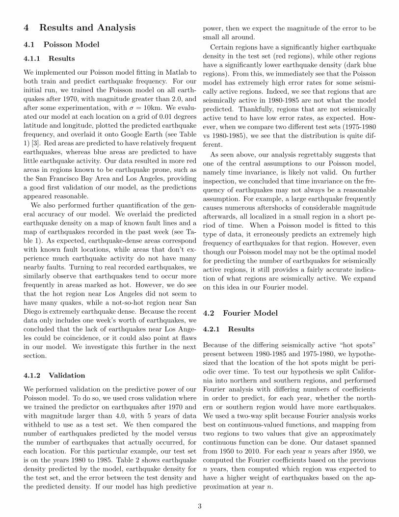
We implemented our Poisson model fitting in Matlab toboth train and predict earthquake frequency. For ourinitial run, we trained the Poisson model on all earth-quakes after 1970, with magnitude greater than 2.0, andafter some experimentation, with σ = 10km. We evalu-ated our model at each location on a grid of 0.01 degreeslatitude and longitude, plotted the predicted earthquakefrequency, and overlaid it onto Google Earth (see Table1) [3]. Red areas are predicted to have relatively frequentearthquakes, whereas blue areas are predicted to havelittle earthquake activity. Our data resulted in more redareas in regions known to be earthquake prone, such asthe San Francisco Bay Area and Los Angeles, providinga good first validation of our model, as the predictionsappeared reasonable.

We also performed further quantification of the gen-eral accuracy of our model. We overlaid the predictedearthquake density on a map of known fault lines and amap of earthquakes recorded in the past week (see Ta-ble 1). As expected, earthquake-dense areas correspondwith known fault locations, while areas that don’t ex-perience much earthquake activity do not have manynearby faults. Turning to real recorded earthquakes, wesimilarly observe that earthquakes tend to occur morefrequently in areas marked as hot. However, we do seethat the hot region near Los Angeles did not seem tohave many quakes, while a not-so-hot region near SanDiego is extremely earthquake dense. Because the recentdata only includes one week’s worth of earthquakes, weconcluded that the lack of earthquakes near Los Ange-les could be coincidence, or it could also point at flawsin our model. We investigate this further in the nextsection.

4.1.2 Validation

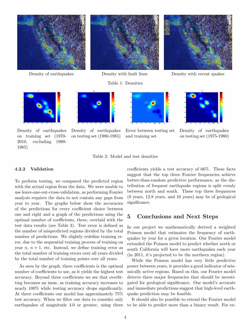
We performed validation on the predictive power of ourPoisson model. To do so, we used cross validation wherewe trained the predictor on earthquakes after 1970 andwith magnitude larger than 4.0, with 5 years of datawithheld to use as a test set. We then compared thenumber of earthquakes predicted by the model versusthe number of earthquakes that actually occurred, foreach location. For this particular example, our test setis on the years 1980 to 1985. Table 2 shows earthquakedensity predicted by the model, earthquake density forthe test set, and the error between the test density andthe predicted density. If our model has high predictive

power, then we expect the magnitude of the error to besmall all around.

Certain regions have a significantly higher earthquakedensity in the test set (red regions), while other regionshave a significantly lower earthquake density (dark blueregions). From this, we immediately see that the Poissonmodel has extremely high error rates for some seismi-cally active regions. Indeed, we see that regions that areseismically active in 1980-1985 are not what the modelpredicted. Thankfully, regions that are not seismicallyactive tend to have low error rates, as expected. How-ever, when we compare two different test sets (1975-1980vs 1980-1985), we see that the distribution is quite dif-ferent.

As seen above, our analysis regrettably suggests thatone of the central assumptions to our Poisson model,namely time invariance, is likely not valid. On furtherinspection, we concluded that time invariance on the fre-quency of earthquakes may not always be a reasonableassumption. For example, a large earthquake frequentlycauses numerous aftershocks of considerable magnitudeafterwards, all localized in a small region in a short pe-riod of time. When a Poisson model is fitted to thistype of data, it erroneously predicts an extremely highfrequency of earthquakes for that region. However, eventhough our Poisson model may not be the optimal modelfor predicting the number of earthquakes for seismicallyactive regions, it still provides a fairly accurate indica-tion of what regions are seismically active. We expandon this idea in our Fourier model.

4.2 Fourier Model

4.2.1 Results

Because of the differing seismically active “hot spots”present between 1980-1985 and 1975-1980, we hypothe-sized that the location of the hot spots might be peri-odic over time. To test our hypothesis we split Califor-nia into northern and southern regions, and performedFourier analysis with differing numbers of coefficientsin order to predict, for each year, whether the north-ern or southern region would have more earthquakes.We used a two-way split because Fourier analysis worksbest on continuous-valued functions, and mapping fromtwo regions to two values that give an approximatelycontinuous function can be done. Our dataset spannedfrom 1950 to 2010. For each year n years after 1950, wecomputed the Fourier coefficients based on the previousn years, then computed which region was expected tohave a higher weight of earthquakes based on the ap-proximation at year n.

3

Density of earthquakes Density with fault lines Density with recent quakes

Table 1: Densities

Density of earthquakeson training set (1970-2010, excluding 1980-1985)

Density of earthquakeson testing set (1980-1985)

Error between testing setand training set

Density of earthquakeson testing set (1975-1980)

Table 2: Model and test densities

4.2.2 Validation

To perform testing, we compared the predicted regionwith the actual region from the data. We were unable touse leave-one-out-cross-validation, as performing Fourieranalysis requires the data to not contain any gaps fromyear to year. The graphs below show the accuraciesof the predictions for every coefficient choice betweenone and eight and a graph of the predictions using theoptimal number of coefficients, three, overlaid with thetest data results (see Table 3). Test error is defined asthe number of mispredicted regions divided by the totalnumber of predictions. We slightly redefine training er-ror, due to the sequential training process of training onyear n, n + 1, etc. Instead, we define training error asthe total number of training errors over all years dividedby the total number of training points over all years.

As seen by the graph, three coefficients is the optimalnumber of coefficients to use, as it yields the highest testaccuracy. Beyond three coefficients we see that overfit-ting becomes an issue, as training accuracy increases tonearly 100% while testing accuracy drops significantly.At three coefficients our model has approximately 75%test accuracy. When we filter our data to consider onlyearthquakes of magnitude 4.0 or greater, using three

coefficients yields a test accuracy of 66%. These factssuggest that the top three Fourier frequencies achievebetter-than-random predictive performance, as the dis-tribution of frequent earthquake regions is split evenlybetween north and south. These top three frequences(8 years, 12.8 years, and 16 years) may be of geologicalsignificance.

5 Conclusions and Next Steps

In our project we mathematically derived a weightedPoisson model that estimates the frequency of earth-quakes by year for a given location. Our Fourier modelextended the Poisson model to predict whether north orsouth California will have more earthquakes each year(in 2011, it’s projected to be the northern region).

While the Poisson model has very little predictivepower between years, it provides a good indicator of seis-mically active regions. Based on this, our Fourier modeldetects three major frequencies that should be investi-gated for geological significance. Our model’s accurateand immediate predictions suggest that high-level earth-quake prediction may be feasible.

It should also be possible to extend the Fourier modelto be able to predict more than a binary result. For ex-

4

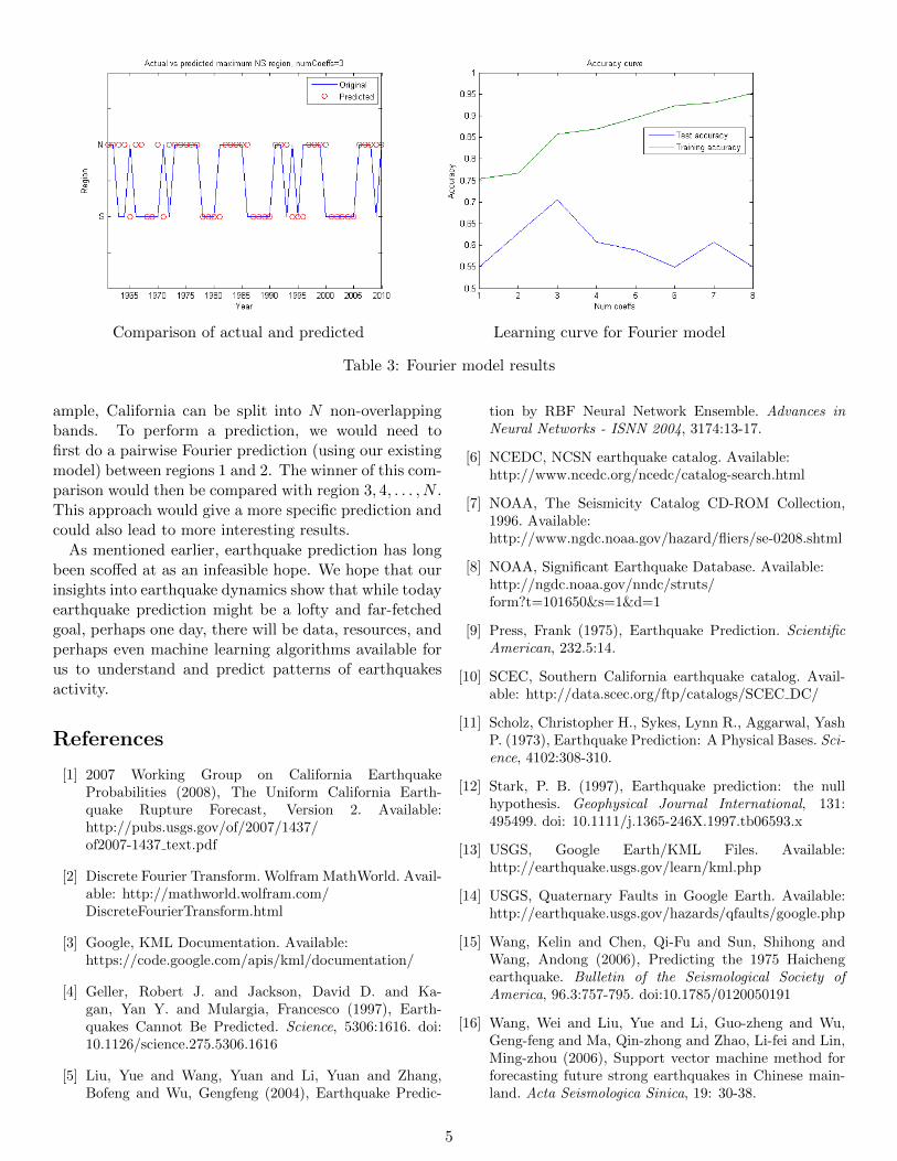
Comparison of actual and predicted Learning curve for Fourier model

Table 3: Fourier model results

ample, California can be split into N non-overlappingbands. To perform a prediction, we would need tofirst do a pairwise Fourier prediction (using our existingmodel) between regions 1 and 2. The winner of this com-parison would then be compared with region 3, 4, . . . , N .This approach would give a more specific prediction andcould also lead to more interesting results.

As mentioned earlier, earthquake prediction has longbeen scoffed at as an infeasible hope. We hope that ourinsights into earthquake dynamics show that while todayearthquake prediction might be a lofty and far-fetchedgoal, perhaps one day, there will be data, resources, andperhaps even machine learning algorithms available forus to understand and predict patterns of earthquakesactivity.

References

[1] 2007 Working Group on California EarthquakeProbabilities (2008), The Uniform California Earth-quake Rupture Forecast, Version 2. Available:http://pubs.usgs.gov/of/2007/1437/of2007-1437 text.pdf

[2] Discrete Fourier Transform. Wolfram MathWorld. Avail-able: http://mathworld.wolfram.com/DiscreteFourierTransform.html

[3] Google, KML Documentation. Available:https://code.google.com/apis/kml/documentation/

[4] Geller, Robert J. and Jackson, David D. and Ka-gan, Yan Y. and Mulargia, Francesco (1997), Earth-quakes Cannot Be Predicted. Science, 5306:1616. doi:10.1126/science.275.5306.1616

[5] Liu, Yue and Wang, Yuan and Li, Yuan and Zhang,Bofeng and Wu, Gengfeng (2004), Earthquake Predic-

tion by RBF Neural Network Ensemble. Advances inNeural Networks - ISNN 2004, 3174:13-17.

[6] NCEDC, NCSN earthquake catalog. Available:http://www.ncedc.org/ncedc/catalog-search.html

[7] NOAA, The Seismicity Catalog CD-ROM Collection,1996. Available:http://www.ngdc.noaa.gov/hazard/fliers/se-0208.shtml

[8] NOAA, Significant Earthquake Database. Available:http://ngdc.noaa.gov/nndc/struts/form?t=101650&s=1&d=1

[9] Press, Frank (1975), Earthquake Prediction. ScientificAmerican, 232.5:14.

[10] SCEC, Southern California earthquake catalog. Avail-able: http://data.scec.org/ftp/catalogs/SCEC DC/

[11] Scholz, Christopher H., Sykes, Lynn R., Aggarwal, YashP. (1973), Earthquake Prediction: A Physical Bases. Sci-ence, 4102:308-310.

[12] Stark, P. B. (1997), Earthquake prediction: the nullhypothesis. Geophysical Journal International, 131:495499. doi: 10.1111/j.1365-246X.1997.tb06593.x

[13] USGS, Google Earth/KML Files. Available:http://earthquake.usgs.gov/learn/kml.php

[14] USGS, Quaternary Faults in Google Earth. Available:http://earthquake.usgs.gov/hazards/qfaults/google.php

[15] Wang, Kelin and Chen, Qi-Fu and Sun, Shihong andWang, Andong (2006), Predicting the 1975 Haichengearthquake. Bulletin of the Seismological Society ofAmerica, 96.3:757-795. doi:10.1785/0120050191

[16] Wang, Wei and Liu, Yue and Li, Guo-zheng and Wu,Geng-feng and Ma, Qin-zhong and Zhao, Li-fei and Lin,Ming-zhou (2006), Support vector machine method forforecasting future strong earthquakes in Chinese main-land. Acta Seismologica Sinica, 19: 30-38.

5