Enhancing trajectory tracking for a class of process control problems using iterative learning

Engineering Applications of Artificial Intelligence 15 (2002) 53–64

Enhancing trajectory tracking for a class of process control problemsusing iterative learning

Jian-Xin Xu*, Tong-Heng Lee, Ying Tan

Department of Electrical Engineering, National University of Singapore, 10 Kent Ridge Crescent, Singapore 119260, Singapore

Abstract

A method of enhancing tracking in repetitive processes, which can be approximated by a first-order plus dead-time model is

presented. Enhancement is achieved through filter-based iterative learning control (ILC). The design of the ILC parameters is

conducted in frequency domain, which guarantees the convergence property in iteration domain. The filter-based ILC can be easily

added to existing control systems. To clearly demonstrate the features of the proposed ILC, a water heating process under a PI

controller is used as a testbed. The empirical results show improved tracking performance with iterative learning. r 2002 Elsevier

Science Ltd. All rights reserved.

Keywords: Enhance tracking; Filter-based iterative learning control; Frequency convergence analysis

1. Introduction

Trajectory tracking, whose primary control target isto track the a specified profile as tightly as possible infinite time interval, is very common in both processcontrol and motion control problems, e.g. temperaturecontrol of a chemical reactor in pharmaceutic industry,or velocity control of an industrial robot in weldingprocess. In practice the most widely used controlschemes in industries are still PI or PID controllerswith modifications, owing to the simplicity, easy tuning,and satisfactory performance (Sepehri et al., 1997;Isaksson and Graebe, 1999; Wang and Shao, 2000).On the other hand, many advanced control schemeshave been proposed to handle complicated controlproblems. Nevertheless, it is still a challenging controlproblem when the perfect trajectory tracking is con-cerned, i.e. how to achieve satisfactory tracking perfor-mance when the process is under transient motion overthe entire operation period. Most advanced controlschemes can only achieve perfect tracking asymptoti-cally—the initial tracking will be conspicuously poorwithin the finite interval. PI or PID control schemes inmost cases can only warrant a zero steady-state error.There are many industrial processes under batch

operations, which by virtue are repeated many times

with the same desired tracking profile. The sametracking performance will thus be observed, albeit withhindsight from previous operations. Clearly, thesecontinual repetitions make it conceivable to improvetracking, potentially over the entire task duration, byusing information from past operations.To enhance tracking in repeated operations, ILC

schemes developed hitherto well cater to the needs(Arimoto et al., 1984; Bien and Xu, 1998; Kuc et al.,1992; Lee and Bien, 1997; Lee et al., 1994; Longman,1998; Moore, 1998; Phan and Juang, 1996; Lee et al.,2000; Wang, 2000). ILC uses repetitions as experience toimprove tracking without exact system knowledge andbecomes one of the most active fields in intelligentcontrol and system control. ILC differers from mostexisting control methods in the sense that it exploitsevery possibility to incorporate past control informa-tion, such as tracking errors and control input signals,into the construction of the present control action (Xuet al., 2000). Numeric processing on those acquiredsignals yields a kind of new feed-forward compensation,which differs from most existing feed-forward compen-sations that are highly model based. Comparing withmany feed-forward compensation schemes, ILC require-ments are minimal—a memory storage for past dataplus some simple data operations to derive the feed-forward signal. With its utmost simplicity, ILC can veryeasily be added on top of existing (predominantly PIDbatch) facilities without any hassle at all.

*Corresponding author. Tel.: +65-874-2566; fax: +65-779-1103.

E-mail address: [email protected] (J.-X. Xu).

0952-1976/02/$ - see front matter r 2002 Elsevier Science Ltd. All rights reserved.

PII: S 0 9 5 2 - 1 9 7 6 ( 0 2 ) 0 0 0 0 8 - 8

In this paper, ILC is employed to enhance theperformance of a kind of process dynamics, which canbe characterized more or less by the first-order plus deadtime (FOPDT) model. The approximated model isusually obtained from the empirical results. It has beenshown that this approximation model, though verysimple, stands near 60 years and is still widely adopted(Seborg et al., 1989). Based upon this FOPDT, thefamous Zieger/Nichols tuning method (Ziegler andNichols, 1942) was developed and nowadays becomean indispensable part of control textbooks (Ogata, 1997).However, when higher tracking performance is

required, feedback and feed-forward compensationsbased on FOPFT model may not be sufficient due tothe limited modeling accuracy. In such circumstance,ILC provides a unique alternative: reconstruct andcapture the desired control profile iteratively throughpast control actions, as far as the process is repeatableover the finite time interval. In this paper, the filter-based learning control scheme is incorporated with PIcontrol in order to improve the transient performance intime domain.The filter-based ILC scheme is proven to converge to

the desired control input in frequency domain within thebandwidth of interest. The bandwidth of interest can beeasily estimated using the approximated FOPDT model.The proposed ILC scheme simply involves two para-meters—the filter length and the learning gain, both canbe easily tuned using the approximated model. Also, thisscheme is practically robust to random system noiseowing to its non-causal zero-phase filtering nature. Awater heating plant is employed as a testbed to illustratethe effectiveness of the proposed filter-based learningscheme.The paper is organized as follows. Section 2

formulates the control problem of FOPDT in general,and the modeling of a water heating plant in particular.Section 3 gives an overview of filter-based ILC with itsconvergence analysis in frequency domain. Section 4details the controller design work and the experimentalresults. From these results, a modified ILC scheme withprofile segmentation and feed-forward initialization, isused to improve tracking performance even further.Finally, Section 5 concludes the paper.

2. Problem formulation

2.1. FOPDT model and PID control

The FOPDT model, has been widely used inindustries to approximate various kinds of type 0processes

GðsÞ ¼Ke�ts

1þ sTa; ð1Þ

where K is the plant steady-state gain, Ta is the apparenttime constant and t is the apparent dead time. There aremainly two reasons accounting for the popularity ofFOPDT model. The first is its extremely simple structureassociated with only three parameters which can beeasily calculated through empirical tests, for example asimple open-loop step response (Ogata, 1997). Thesecond is the well developed PI and PID autotuningrules which provide a simple and effective way forsetting controller parameters (Ziegler and Nichols, 1942;Hang et al., 1991).FOPDT model provides a very convenient way to

facilitate the PI/PID controller setting, regardless of theexistence of nonlinear factors, higher-order dynamics, oreven distributed parametric dynamics, etc. In practicethe FOPDT model based PI/PID control has beeneffectively applied to two kinds of control problems.One is the regulation problem where the objective is tomaintain the operating point, and another is the set-point control problem where the objective is to achieve apre-specified step response with balanced performanceamong settling time, overshoot and rising time. How-ever, this simple control strategy, which is based onsimple model approximation such as FOPDT, andsimple control schemes such as PID, may not be suitablefor more complicated control tasks with high trackingprecision requirement. Consider a control target: track-ing a temperature profile as shown in Fig. 1. This is thesimplest trajectory consisting of two segments: a rampand a level, starting at t ¼ 0 and ending at t ¼ 3600 s:A few problems arise when such a trajectory tacking

task is to be fulfilled. First, a single integrator isinadequate to follow a ramp signal. Adding moreintegrators will adversely degrade the system perfor-mance due to the extra phase lag. Second, even if the

T = 0.0197t

+ 24.5

T = 60

24

29

34

39

44

49

54

59

64

0 1000 2000 3000Time(s)

T/ ˚C

1800

Fig. 1. Desired temperature profile.

J.-X. Xu et al. / Engineering Applications of Artificial Intelligence 15 (2002) 53–6454

controller is able to follow the reference in the steadystate, the transient performance will be poor, because ofthe finite tracking period. Third, since only an approx-imate FOPDT model is available, many advancedcontrol schemes, which require much of the modelingknowledge, cannot be applied. Accurate modeling, onthe other hand, is time consuming, costly, and usually atougher problem than control.It is worthy to point out, when a control task is

performed repeatedly, we gain extra information from anew source: past control input and tracking errorprofiles. Different from most control strategies, iterativelearning control explores the possibility of fully utilizingthis kind of system information, in the sequel enhancingtracking for the next run. An immediate advantage is,the need for process model knowledge can be signifi-cantly reduced. We will show later that, in order todesign an ILC in frequency domain based on the simpleFOPDT model, it is sufficient to know approximatelythe bandwidth of the desired control profile. Anotheradvantage is, that we can retain the auto-tuned orheuristically tuned PI/PID, and simply add the ILCmechanism. In this way the characteristics of the existingfeedback controller can be well reserved, and ILCprovides extra feed-forward compensation.

2.2. Modeling the water heating plant

To facilitate the discussions on modeling and controlin general, and verify the effectiveness of ILC withFOPDT in particular, a water heating process is usedthroughout the paper. Fig. 2 is a schematic diagramshowing the relevant portions of the water heating plant.Water from Tank A is pumped (N1) through a heatexchanger as the cooling stream. The heating stream onthe other side of the exchanger is supplied from a heatedreservoir. This heated stream is pumped (N2) throughthe exchanger before returning to the reservoir where itis heated by a heating rod (PWR). A distributed modelbased on physical principles gives a first-order partialdifferential equation (PDE), as shown in Appendix A.Fig. 3 shows the responses obtained from the experi-ment with the actual plant, and the simulation with the

PDE model, to a step input of 200 W at the heater (theheater is switched to 200 W at t ¼ 0 s and then switchedoff at t ¼ 12500 s).Both the simulation and the experimental responses

show that the water heating plant can be effectivelyapproximated by the following FOPDT system:

GðsÞ ¼T2ðsÞ

PWRðsÞ¼

0:1390

2865 sþ 1e�50s: ð2Þ

The dead-time t ¼ 50 s is measured in experiment. Sincethe process can be approximated by FOPDT, normallya PI controller is designed to realize a set-point controltask. The PI controller can be tuned using relayexperiments (Astrom and Hagglund, 1988) accordingto the Ziegler Nichols rule. The ultimate gain Ku andperiod Pu are 125:01C=W and 512:2 s; giving the P gainand integral time to be Kp ¼ Ku=2:2 ¼ 56:81C=W andTi ¼ Pu=1:2 ¼ 426:8 s: Now let the target trajectory bethe piece-wise smooth temperature profile shown inFig. 1. The control objective is for T2 (water tempera-ture in the heated reservoir) to track the trajectory asclosely as possible over its entire duration, by varyingthe input to the heater (PWR). Both pumps (N1 & N2)are maintained at pre-set values throughout the run. Thetracking response under PI control is shown in Fig. 4.From the experimental result we can observe the large

tracking discrepancy at the initial stages of the ramp andlevel segments. The control system is not able to makequick response to the variations of the target trajectory,due to the inherent phase lag nature of the process andthe feedback controller. Such a phase lag could havestrong influence to the transient performance. The mosteffective way to overcome the difficulty incurred by thesystem delay is to incorporate a feed-forward compen-sation, which in the ideal case should be able to providethe desired control input profile udðtÞ: For the waterheating process, the estimated control input profile #udðtÞ;

Fig. 2. Schematic diagram of a water heating plant. Fig. 3. Model and plant response to 200 W step.

J.-X. Xu et al. / Engineering Applications of Artificial Intelligence 15 (2002) 53–64 55

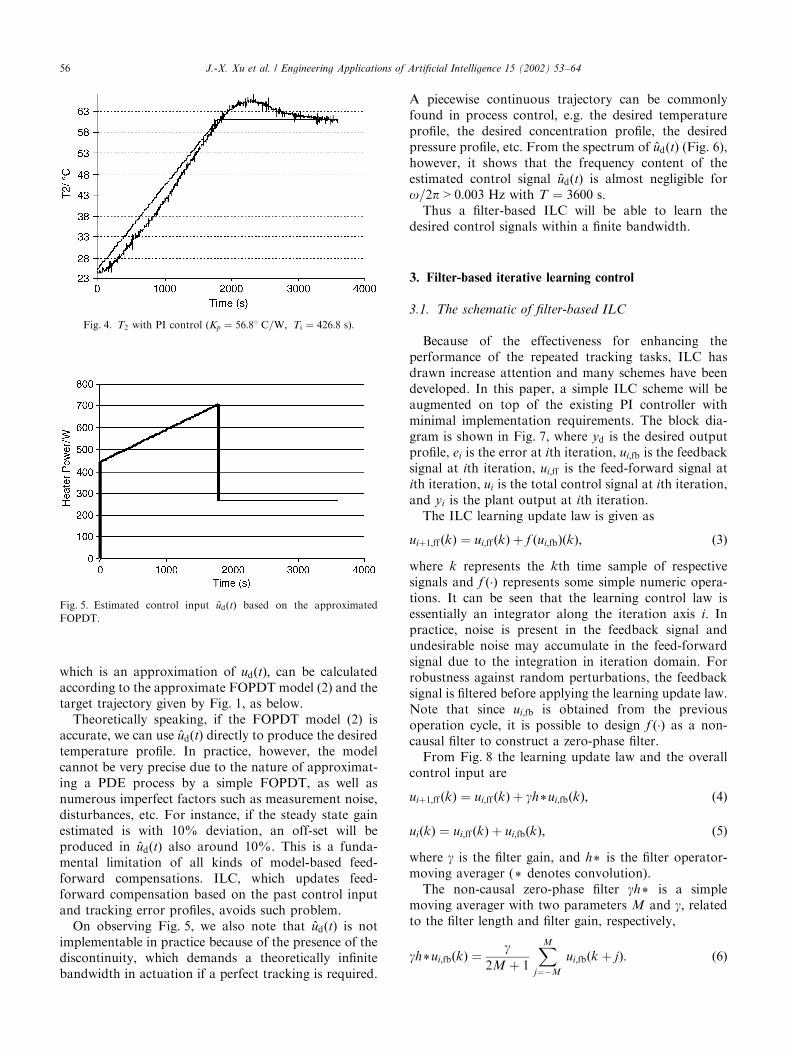
which is an approximation of udðtÞ; can be calculatedaccording to the approximate FOPDT model (2) and thetarget trajectory given by Fig. 1, as below.Theoretically speaking, if the FOPDT model (2) is

accurate, we can use #udðtÞ directly to produce the desiredtemperature profile. In practice, however, the modelcannot be very precise due to the nature of approximat-ing a PDE process by a simple FOPDT, as well asnumerous imperfect factors such as measurement noise,disturbances, etc. For instance, if the steady state gainestimated is with 10% deviation, an off-set will beproduced in #udðtÞ also around 10%. This is a funda-mental limitation of all kinds of model-based feed-forward compensations. ILC, which updates feed-forward compensation based on the past control inputand tracking error profiles, avoids such problem.On observing Fig. 5, we also note that #udðtÞ is not

implementable in practice because of the presence of thediscontinuity, which demands a theoretically infinitebandwidth in actuation if a perfect tracking is required.

A piecewise continuous trajectory can be commonlyfound in process control, e.g. the desired temperatureprofile, the desired concentration profile, the desiredpressure profile, etc. From the spectrum of #udðtÞ (Fig. 6),however, it shows that the frequency content of theestimated control signal #udðtÞ is almost negligible foro=2p > 0:003 Hz with T ¼ 3600 s:Thus a filter-based ILC will be able to learn the

desired control signals within a finite bandwidth.

3. Filter-based iterative learning control

3.1. The schematic of filter-based ILC

Because of the effectiveness for enhancing theperformance of the repeated tracking tasks, ILC hasdrawn increase attention and many schemes have beendeveloped. In this paper, a simple ILC scheme will beaugmented on top of the existing PI controller withminimal implementation requirements. The block dia-gram is shown in Fig. 7, where yd is the desired outputprofile, ei is the error at ith iteration, ui;fb is the feedbacksignal at ith iteration, ui;ff is the feed-forward signal atith iteration, ui is the total control signal at ith iteration,and yi is the plant output at ith iteration.The ILC learning update law is given as

uiþ1;ff ðkÞ ¼ ui;ff ðkÞ þ f ðui;fbÞðkÞ; ð3Þ

where k represents the kth time sample of respectivesignals and f ð�Þ represents some simple numeric opera-tions. It can be seen that the learning control law isessentially an integrator along the iteration axis i: Inpractice, noise is present in the feedback signal andundesirable noise may accumulate in the feed-forwardsignal due to the integration in iteration domain. Forrobustness against random perturbations, the feedbacksignal is filtered before applying the learning update law.Note that since ui;fb is obtained from the previousoperation cycle, it is possible to design f ð�Þ as a non-causal filter to construct a zero-phase filter.From Fig. 8 the learning update law and the overall

control input are

uiþ1;ff ðkÞ ¼ ui;ff ðkÞ þ gh*ui;fbðkÞ; ð4Þ

uiðkÞ ¼ ui;ff ðkÞ þ ui;fbðkÞ; ð5Þ

where g is the filter gain, and h* is the filter operator-moving averager (* denotes convolution).The non-causal zero-phase filter gh* is a simple

moving averager with two parameters M and g; relatedto the filter length and filter gain, respectively,

gh*ui;fbðkÞ ¼g

2M þ 1

XM

j¼�M

ui;fbðk þ jÞ: ð6Þ

Fig. 4. T2 with PI control (Kp ¼ 56:81 C=W; Ti ¼ 426:8 sÞ:

Fig. 5. Estimated control input #udðtÞ based on the approximated

FOPDT.


Memory

PI Controller

Plantyd

ei

ui,fb

ui,ff

yi

+

++

-ui

Fig. 7. Block diagram of ILC scheme used.

� h*

Memory - +Plant

PI

uffi-1

+

++

+

uiuffi yi

ufbi

yd

(i - 1)th iteration

(i+1)th iteration

ufbi-1

ei

Fig. 8. Block diagram of filter-based ILC scheme.

10_3 10

_2 10_1

0

10

20

30

40

50

60

80

70

90

100

Fig. 6. Spectrum of #udðtÞ:


Basically, the filter-based ILC attempts to store thedesired control signal in the memory bank as the feed-forward signal. With convergence, the feed-forwardsignal will tend to the desired control signal so that, intime, it will relieve the burden of the feedback controller.As for all ILC schemes, it is important that theplant output converges to the desired profile alongwith iterations. This is shown in the convergenceanalysis.

3.2. Frequency domain convergence analysis of

filter-based ILC

Since there exists physical frequency limitation ofcontrol input (PWR), it is sufficient and convenient toprovide frequency domain convergence analysis in finitefrequency range for the systematic design (Burdet et al.,1998). Comparing with the time domain analysis,frequency domain analysis offers more insight into theeffects of the plant, the PI controller and the learningfilter on ILC performance and allows for the systematicdesign of M and g based on the linearized FOPDT plantmodel.Since ILC can only be implemented digitally, the

frequency analysis should actually be done on sampled-date systems. When the sampling frequency is muchfaster compared to the system bandwidth, the aliasingproblem is negligible and a zero-order hold filter willvery nearly reconstruct the correct output signal to theplant. Assuming this is so, the analysis can proceed asthough for continuous systems.Consider linear systems with GbðjoÞ and GoðjoÞ as the

transfer functions of the feedback controller and theopen-loop plant, respectively. The closed-loop transferfunction is

GcðjoÞ ¼GbðjoÞGoðjoÞ

1þ GbðjoÞGoðjoÞ: ð7Þ

Writing the learning update law (4) in the frequencydomain gives

Uiþ1;ff ðjoÞ ¼ Ui;ff ðjoÞ þ gHðjoÞUi;fbðjoÞ: ð8Þ

In the following we show that the learning signalUiþ1;ff ðjoÞ will approach the desired control input udðtÞas the iteration evolves. To show this we need toeliminate Ui;fbðjoÞ: Let us omit jo for brevity. From (7),we have the following factor:

Yd ¼ GoUd

¼Gcð1þ GbGoÞ

GbUd

) Ud ¼Gb

Gcð1þ GbGoÞYd; ð9Þ

where Yd and Ud are the Fourier transforms of thedesired profile ydðtÞ and the desired control input udðtÞ;

respectively. Note that

Ui;fb ¼ GbðYd � YiÞ

¼ GbGoðUd � Ui;ff � Ui;fbÞ

) Ui;fb ¼GbGo

ð1þ GbGoÞðUd � Ui;ff Þ

¼ GcðUd � Ui;ff Þ: ð10Þ

Substituting (9) into the above relation, Ui;fb can bewritten as

Ui;fb ¼Gb

1þ GbGoYd � GcUi;ff : ð11Þ

Thus (8) becomes the following difference equation inthe frequency domain consisting of Ui;ff and Ud:

Uiþ1;ff ¼ ð1� gHGcÞUi;ff þ gHGcUd: ð12Þ

Iterating the relationship (12) by i times, we have

Uiþ1;ff ¼ ð1� gHGcÞiU0;ff þ gHGcUd½1þ ð1� gHGcÞ

þ?þ ð1� gHGcÞi

¼ ð1� gHGcÞiU0;ff þ gHGcUd

1� ð1� gHGcÞi

1� ð1� gHGcÞ

¼ ð1� gHGcÞiU0;ff þ ½1� ð1� gHGcÞ

iUd: ð13Þ

Clearly, the convergence condition is

j1� gHðjoÞGcðjoÞjo1 8opob; ð14Þ

where ob is the upper bound of #UdðoÞ: When theconvergence condition (14) is satisfied, the convergedvalue is

limi-N

Ui;ff ¼ Ud: ð15Þ

From (12), it is interesting to observe that Gc acts likea filter on ud while gH is similar to an ‘‘equaliser’’ usedto compensate the ‘‘channel’’ filter. In particular, whenH or Gc ¼ 0; the feed-forward signal maintains at itsinitial value, i.e. learning will not take place at thesefiltered frequencies. This is a desirable property in higherfrequency band (above ob) dominated by noise. UsuallyGc is the existing closed-loop control system designedwithout considering the learning function. Hence H isthe only anti-noise filter, which should get rid of anyfrequencies above ob; and retain the useful frequencycomponents in ud: As udðtÞ is unknown, the frequencydomain design can be based on the information of #udðtÞ;as we shall show in the next section.In linear systems, if the Nyquist curve of 1� gHGc

falls within the unit circle for all frequencies in #udðtÞ;then the (14) is satisfied. Ideally, the Nyquist curveshould be close to the origin to give a faster convergencerate of learning for all relevant frequencies.


4. Temperature control of the water heating plant

4.1. Experimental setup

Fig. 9 shows the hardware block diagram of the waterheating plant—PCT23 Process Plant Trainer. In theexperiment, the console is interfaced to a PC via theMetraByte DAS-16 AD/DA card. The plant is con-trolled by a user-written C DOS program in the PC.This program is interrupt driven and serves to commandthe required control signal to the plant as well as collectand store plant readings. The PI control and reading aredone at a rate of 1 Hz; which is more than adequate forthe system and the ILC bandwidths. Note that thebandwidth of the desired control input has beencalculated based on the estimated #ud; which is ob ¼0:003 Hz (Fig. 6).

4.2. Design of ILC parameters M and g

Filter-based ILC is used to augment the PI feedbackcontroller. M is designed with two opposing considera-tions in mind—high frequency noise rejection andlearning rate for opob: Since M is the length of theaveraging filter, the larger the M; the lower the filterbandwidth, hence the more effective is the noiserejection. On the other hand, as seen in the convergenceanalysis, H and Gc; both being low-pass filters, limit thelearning rate at higher frequencies. Thus, a large M andhence a small filter bandwidth is detrimental to higherfrequency learning.For the plant, the bandwidth of Gc is 0:0045 rad=s;

which is slightly above ob: To reduce the impact of H onhigher frequency learning nearby ob; H can be designedsuch that its bandwidth is slightly larger than Gc: SettingM ¼ 10 and 100 give filter bandwidths of 0:14 and0:014 rad=s; respectively. Obviously, M ¼ 100 willprovide better noise rejection. At the same time, M ¼100 also gives a bandwidth that is slightly larger than Gc:Thus, M ¼ 100 is chosen. The noise rejection effective-ness of this filter will be verified from empirical resultslater.From the bandwidths of Gc and H ; it is seen that the

sampling frequency of 1 Hz is adequate to preventaliasing in the signals. Thus, frequency convergenceanalysis presented in Section 3 is applicable and thedesign of g can be done using Nyquist plots. Using the

FOPDT model (2) and the PI controller, the Nyquistplot (Fig. 10) of 1� gHGc with M ¼ 100 is obtained forg ¼ 0:25; 0:50; 0:75 and 1:00: Note that the size of thecurves, i.e. the heart-shaped lobe, increases with g: Also,each curve starts at 1þ 0j for o ¼ �pfs and tracesclockwise back to 1þ 0j for o ¼ pfs where fs ¼ 1 Hz isthe sampling interval.It can be seen that all the curves have portions falling

outside the unit circle. Thus, convergence is notguaranteed for o=2p > 0:0046; 0.0040, 0.0034 and0:0028 Hz for g ¼ 0:25; 0.5, 0.75 and 1, respectively.However, Fig. 6 shows that the frequency content of theestimated control signal #udðtÞ is almost negligible foro=2p > 0:003 Hz with T ¼ 3600 s: As a tradeoff be-tween stability (location near to unit circle coveringmore frequencies) and learning rate (proximity toorigin), g ¼ 0:5 is chosen.

4.3. Filter-based ILC results for g ¼ 0:5 and M ¼ 100

Comparing with the pure PI control (Fig. 4), aftersimple enhancement with the easily implemented ILC,the repetitive system shows vast tracking improvementsafter eight iterations (Fig. 11). This improvement is alsoobvious from the RMS error trend shown in Fig. 12.In Fig. 11, only a little overshoot and undershoot are

seen at the sharp turn in the output profile. With thelimited bandwidth of Gc; the high frequency componentsat the sharp turn in #udðtÞ (Fig. 5) are filtered out fromui;ff ðtÞ: The lack of these components gives the ‘‘ringing’’at the sharp turn seen in Fig. 13, leading to overshootand undershoot in the output.From Fig. 14, it is also seen that the feed-forward

signal is relatively smooth and noiseless. This implies

PC AD/DAControl Console Plant

Fig. 9. Hardware block diagram of the water heating plant.

0.5

1

1.5

30

210

60

240

90

270

120

300

150

330

180 0

Fig. 10. Nyquist plot of 1� gHGc ðM ¼ 100Þ:


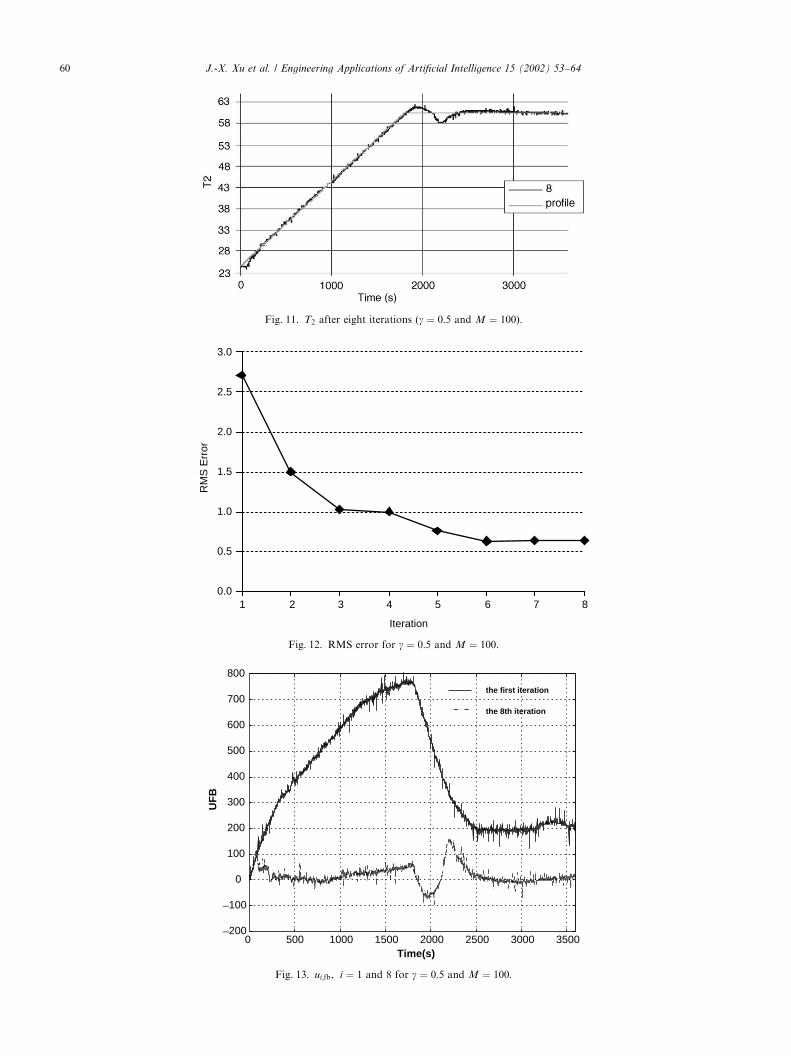
Fig. 11. T2 after eight iterations (g ¼ 0:5 and M ¼ 100Þ:

0.0

0.5

1.0

1.5

2.0

2.5

3.0

1 2 3 4 5 6 7 8

Iteration

RM

S E

rror

Fig. 12. RMS error for g ¼ 0:5 and M ¼ 100:

0 500 1000 1500 2000 2500 3000 3500_200

_100

0

100

200

300

400

500

600

700

800

Time(s)

UF

B

the first iteration

the 8th iteration

Fig. 13. ui;fb; i ¼ 1 and 8 for g ¼ 0:5 and M ¼ 100:


that the ILC filter is effective in rejecting noise, makingthe scheme robust to random perturbations in thesystem.

4.4. Profile segmentation with feed-forward initialization

To improve tracking at the sharp turn, a variation onILC is attempted. From Fig. 5, the desired control ispiecewise smooth—consisting of a ramp segment and alevel segment. Near the turn, due to the ‘‘windowaveraging’’ effect of the ILC filter, the feed-forwardsignal is derived from these two radically differentcontrol efforts—one ‘‘correct’’, the other ‘‘wrong’’. Forexample, when the averaging window is mainly on rampsegment but moving towards the turn point, signalstaken from ramp segment are the ‘‘correct’’ ones andthose from level segment are the ‘‘wrong’’ ones, and viceversa.Thus, the original profile is divided into two entirely

smooth profiles. ILC will proceed separately for eachprofile, meaning that the ILC filter will be applied onlyone side around the sharp turn. At the same time, theintegral part of the PI controller is reset to 0 at the startof each segment. Effectively, it is as though a brand newbatch process is started at the turn.In addition, it is easy to estimate, from the first

iteration, the steady-state control effort required for thelevel segment. At the second iteration, the feed-forwardsignal for level segment is initialized to this estimate.From then on, ILC proceeds normally for all subse-quent iterations, further alleviating any inaccuracy inthe estimate.

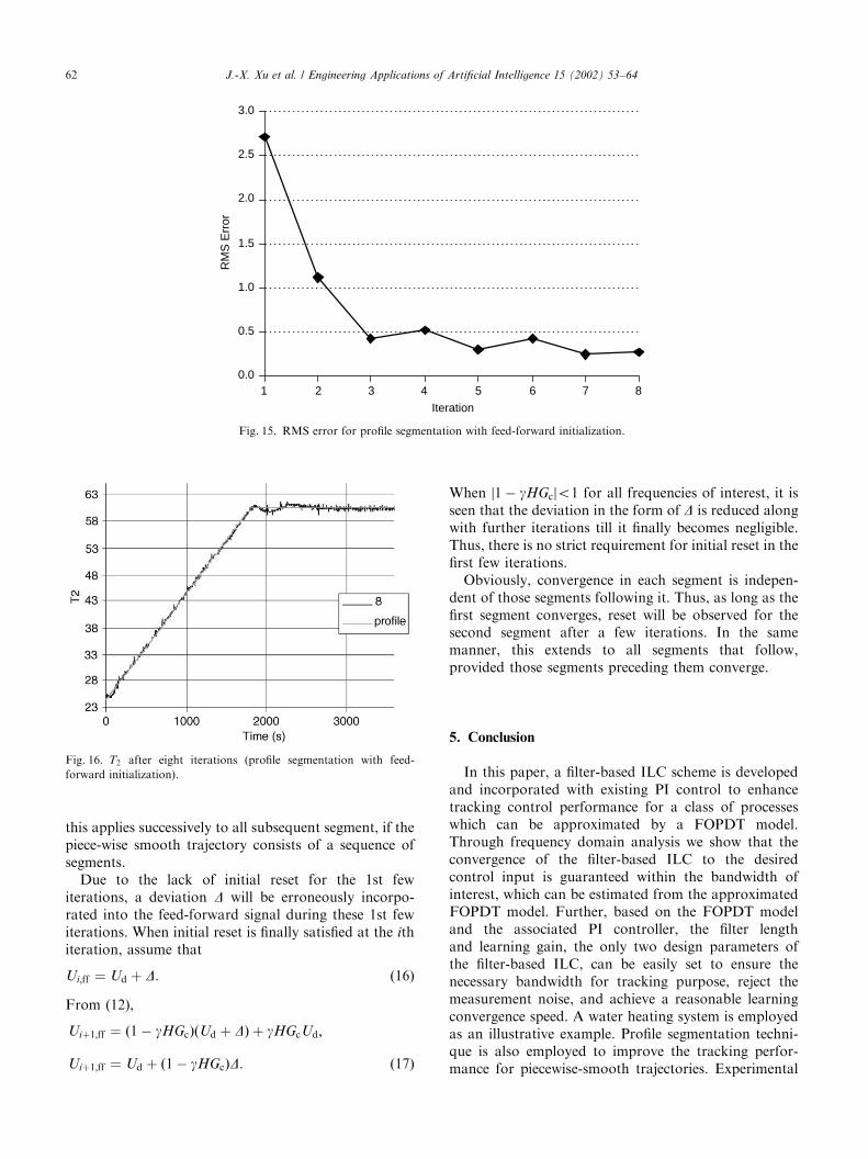
Compared with Fig. 12, the RMS error trend inFig. 15 shows that the improvement from the first to thesecond iteration is more significant owing to the feed-forward initialization. In addition, the error settles to asmaller value.The smaller error can be attributed to better tracking

at the sharp turn as shown in Fig. 16. Comparing toFig. 11, there is very much less overshoot and under-shoot.Through segmentation, the filter’s ‘‘window aver-

aging’’ effect at the turn is eliminated. In general, thesystem closed-loop bandwidth still limits the frequencycomponents to be successfully incorporated into thefeed-forward signal. This limitation is somewhat com-pensated by initializing the feed-forward signal with thecontrol estimate.

4.5. Initial resetting condition

One very important property of ILC is thatinitial plant reset is required—the feed-forward signalis meaningful only if the plant starts from the sameinitial conditions in all iterations, this being known asthe initial reset condition. Obviously, this is notguaranteed with profile segmentation except for thefirst one.Given convergence in the first segment, this problem

occurs for only the first few iterations after which thefirst segment converges to the desired profile so thatreset will be satisfied for the subsequent segment. This isbecause the end point of the 1st segment is exactly theinitial point of the 2nd segment. In the same manner,

0 500 1000 1500 2000 2500 3000 35000

100

200

300

400

500

600

Time(s)

UF

F

the first iteration

the 8th iteration

Fig. 14. ui;ff ; i ¼ 1 and 8 for g ¼ 0:5 and M ¼ 100:


this applies successively to all subsequent segment, if thepiece-wise smooth trajectory consists of a sequence ofsegments.Due to the lack of initial reset for the 1st few

iterations, a deviation D will be erroneously incorpo-rated into the feed-forward signal during these 1st fewiterations. When initial reset is finally satisfied at the ithiteration, assume that

Ui;ff ¼ Ud þ D: ð16Þ

From (12),

Uiþ1;ff ¼ ð1� gHGcÞðUd þ DÞ þ gHGcUd;

Uiþ1;ff ¼ Ud þ ð1� gHGcÞD: ð17Þ

When j1� gHGcjo1 for all frequencies of interest, it isseen that the deviation in the form of D is reduced alongwith further iterations till it finally becomes negligible.Thus, there is no strict requirement for initial reset in thefirst few iterations.Obviously, convergence in each segment is indepen-

dent of those segments following it. Thus, as long as thefirst segment converges, reset will be observed for thesecond segment after a few iterations. In the samemanner, this extends to all segments that follow,provided those segments preceding them converge.

5. Conclusion

In this paper, a filter-based ILC scheme is developedand incorporated with existing PI control to enhancetracking control performance for a class of processeswhich can be approximated by a FOPDT model.Through frequency domain analysis we show that theconvergence of the filter-based ILC to the desiredcontrol input is guaranteed within the bandwidth ofinterest, which can be estimated from the approximatedFOPDT model. Further, based on the FOPDT modeland the associated PI controller, the filter lengthand learning gain, the only two design parameters ofthe filter-based ILC, can be easily set to ensure thenecessary bandwidth for tracking purpose, reject themeasurement noise, and achieve a reasonable learningconvergence speed. A water heating system is employedas an illustrative example. Profile segmentation techni-que is also employed to improve the tracking perfor-mance for piecewise-smooth trajectories. Experimental

0.0

0.5

1.0

1.5

2.0

2.5

3.0

1 2 3 4 5 6 7 8

Iteration

RM

S E

rror

Fig. 15. RMS error for profile segmentation with feed-forward initialization.

Fig. 16. T2 after eight iterations (profile segmentation with feed-

forward initialization).


results clearly show the effectiveness of the proposedmethod.

Acknowledgements

This work is supported by Academic Research Fund,National University of Singapore, Grant No. R-263-000-049-112.

Appendix A

A.1. The physical model of the water heating plant

The plant can be represented in a simplified form asshown in Fig. 17 (Schiesser, 1997). It is assumed thatthere is no heat loss. In the reservoir tank, the followingPDE represents the heating process:

roco@T

@tþ nr

@T

@x

� �¼

PðtÞlrar

; ðA:1Þ

where ro is the density of water, T is the temperature ofreservoir water, co is the specific heat capacity of water,nr is the tangential flow velocity in the reservoir, and P isthe power input of the heater.The heat exchanger is described by the following

equations. In this case, the plate exchanger in thephysical system is modeled as a counter-flow plateexchanger. For the heating stream and cooling streams,respectively,

roco@T1

@tþ ne1

@T1

@x1

� �¼

U

hðT2 � T1Þ;

roco@T2

@tþ ne1

@T2

@x2

� �¼

U

hðT2 � T � 1Þ; ðA:2Þ

where T1 is the heating stream temperature, ne1

is the heating stream flow velocity, T2 is the coolingstream temperature, ne1 is the cooling stream flowvelocity, U is the overall heat transfer coefficient, h isthe height of stream, x1 is the distance from heating

stream inlet, and x2 is the distance from cooling streaminlet.The following initial and boundary conditions apply

for the system:

Reservoir Heat exchangerTðx; t ¼ 0Þ ¼ Trm T1ðx1; t ¼ 0Þ ¼ T2ðx2; t ¼ 0Þ ¼ Trm

Tðx ¼ 0; tÞ ¼ Te T1ðx1 ¼ 0; tÞ ¼ Tr

T2ðx2 ¼ 0; tÞ ¼ Trm

where Trm is the room temperature, Te is the tempera-ture at outlet of heating stream, and Tr is thetemperature at outlet of reservoir.

References

Arimoto, S., Kawamura, S., Miyazaki, F., 1984. Bettering operation of

robots by learning. Journal of Robotic Systems 1 (2), 123–140.

Astrom, K.J., Hagglund, T., 1988. Automatic Tuning of PID

Controllers. Research Triangle Park, NC, Instrument Society of

America.

Bien, Z., Xu, J.X., 1998. Iterative Learning Control—Analysis,

Design, Integration and Applications. Kluwer Academic Publish-

ers, Dordrecht.

Burdet, E., Codourey, A., Rey, L., 1998. Experimental evaluation of

nonlinear adaptive controllers. IEEE Control Systems Magazine 18

(2), 39–47.

Hang, C.C., Astrom, K.J., Ho, W.K., 1991. Refinements of the

Ziegler–Nichols tuning formula. IEE Proceedings D, Control

Theory and Applications 138, 111–119.

Isaksson, A.J., Graebe, S.F., 1999. Analytical PID parameter

expressions for higher order systems. Automatica 35 (6),

1121–1130.

Kuc, Y.Y., Lee, S.J., Nam, K.H., 1992. An iterative learning control

theory for a class of nonlinear dynamic systems. Automatica 28

(10), 1215–1221.

Lee, H.S., Bien, Z., 1997. A note on convergence property of iterative

learning controller with respect to sup norm. Automatica 33,

1591–1593.

Lee, K.S., Bang, S.H., Chang, K.S., 1994. Feedback-assisted iterative

learning control based on an inverse process model. Journal of

Process Control 4 (2), 77–89.

Lee, T.H., Tan, K.K., Huang, S.N., Dou, H.F., 2000. Intelligent

control of precision linear actuators. Engineering Applications of

Artificial Intelligence 13 (6), 671–684.

Longman, R.W., 1998. Designing iterative learning and repetitive

controllers. In: Xu J.-X., Bien Z.Z. (Eds.), Iterative Learning

Control—Analysis, Design, Integration and Application. Kluwer

Academic Publishers, Dordrecht, pp. 107–145.

Moore, K.L., 1998. Iterative Learning Control—An Expository

Overview, Applied & Computational Controls. Signal Processing

and Circuits, 1–42.

Ogata, K., 1997. Modern Control Engineering. Prentice-Hall, Engle-

wood Cliffs, NJ.

Phan, J., Juang, J., 1996. Designs of learning controllers based on an

auto-regressive representation of a linear system. AIAA Journal of

Guidance, Control and Dynamics 19 (2), 355–362.

Schiesser, W.E., 1997. Computational Transport Phenomena: Numer-

ical Methods for the Solution of Transport Problems. Cambridge

University Press, Cambridge, pp. 289–326.

Seborg, D.E., Edgar, T.F., Mellichamp, D.A., 1989. Process Dynamics

and Control. Wiley, New York.

Reservoir

Exchanger

lr

ar

2h

le

Cooling Stream

Heating Stream

Fig. 17. Simplified model of water heating plant.


Sepehri, N., Khayyat, A.A., Heinrichs, B., 1997. Development of a

nonlinear PI controller for accurate positioning of an industrial

hydraulic manipulator. Mechatronics 7 (8), 683–700.

Xu, J.X., Lee, T.H., Chen, Y.Q., 2000. Knowledge learning in discrete-

time control systems. In: Leondes C.T. (Ed.), Knowledge-Base

Systems-Techniques and Applications. Academic Press, New York,

pp. 943–976.

Wang, D.W., 2000. On D-type and P-type ILC designs and anticipatory

approach. International Journal of Control 73 (10), 890–901.

Wang, Y.G., Shao, H.H., 2000. Optimal tuning for PI controller.

Automatica 36 (1), 147–152.

Ziegler, J.B., Nichols, N.B., 1942. Optimum settings for automatic

controllers. Transactions on American Society of Mechanical

Engineering 64, 759–768.


Documents

Enhancing trajectory tracking for a class of process control problems using iterative learning