Embed Size (px)
Citation preview

Faculty of Postgraduate Studies and Scientific Research
German University in Cairo
Enhancing One-Class SupportVector Machines for Unsupervised
Anomaly Detection
A thesis submitted in partial fulfillment of the requirements for the degree
of Master of Science in Computer Science and Engineering
By
Mennatallah Amer
Supervised by
Markus GoldsteinProf. Dr. Andreas Dengel
Prof. Dr. Slim Abdennadher
27 March, 2013


Approval Sheet
This thesis has been approved in partial fulfillment for the degree of Master of Science in
Computer Science and Engineering by the Faculty of Postgraduate Studies and Scientific
Research at the German University in Cairo (G.U.C) on 27th, March 2013.
Markus Goldstein
Researcher
Multimedia Analysis and Data Mining Research Group
German Research Center for Artificial Intelligence, DFKI GmbH
Prof. Dr. Prof. h.c. Andreas Dengel
Full Professor (C4)
Computer Science Department
Technical University Kaiserslautern
Prof. Dr. Slim Abdennadher
Professor
Computer Science and Engineering Department
German University in Cairo

This is to certify that:
(i) the thesis compromises only my original work toward the Masters Degree
(ii) due acknowledgment has been made in the text to all other material used
Mennatallah Amer
27 March, 2013

Acknowledgment
I have had the opportunity to do this work as a result of the ongoing cooperation between
the German University in Cairo (GUC) and the German Research Center for Artificial In-
telligence (DFKI GmbH). After Allah, a lot of people have helped, inspired and supported
me throughout this project. First, I would like to thank my professor, Slim Abennad-
her, for his continuous efforts in putting everything together and for lobbying me into
Computer Science and Engineering to begin with. I am thankful to Prof. Dr. Andreas
Dengel for continuing to believe in the GUC students and establishing this joint cooper-
ation. From an administrative perspective, Dr. Thomas Kieninger and Brigitte Selzer,
facilitated every aspect of our stay in Germany demonstrating exceptional patience and
tolerance to our lengthy paradoxal emails. My supervisor, Markus Goldstein, provided
me with both, the flexibility and the guidance, to define the scope of this work. Then, his
input and trust pushed this work through. I could not have made it through Germany’s
winter without the amazing company of my friends: Maha, Salma, Passant, Sara, Bahaa,
Mohamed Anwar, Mohamed Selim and Yumn. I also had a lot of support and feedback
from my friends in the GUC: Nazly Sabour, Wallas, Ramy Wafa, Hadeer Diwan, Noura
El-Maghawry and Yahia El Gamal. I am very grateful to Dr. Seif Eldawlatly for his
thorough feedback on my work. A special thanks goes to my mum and her incredible
co-workers, especially Eyad, for saving my thesis draft. Surely no words can describe my
love and gratitude for my family for their unconditional love and support. My mum has
been there for me in every step of the way, relentlessly helping, guiding and protecting
me with all her being. My protecting loving father has supported and trusted me with all
my choices, even though they might have seemed incomprehensible at times. My siblings,
Mohamed and Mariam, bring so much cheerfulness, joy and balance to my life.
IV
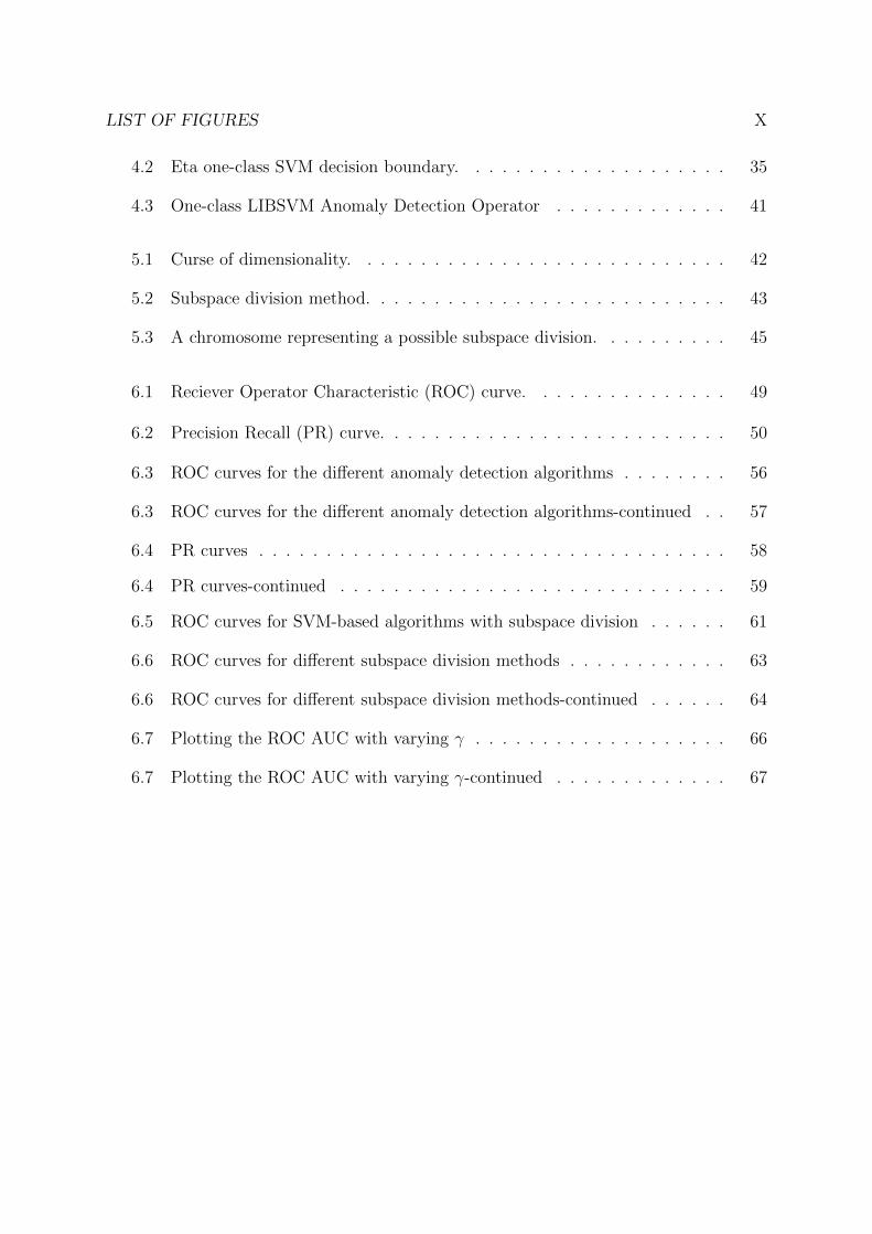
Abstract
Support Vector Machines (SVMs) have been one of the most prominent machine learn-
ing techniques for the past decade. In this thesis, the effectiveness of applying SVMs
for detecting outliers in an unsupervised setting is investigated. Unsupervised anomaly
detection techniques operate directly on an unseen dataset, under the assumption that
outliers are sparsely present in it. One-class SVM, an extension to SVMs for unlabeled
data, can be used for anomaly detection. Even though outliers are accounted for in
one-class SVMs, they greatly influence the learnt model. Hence, two modifications to
one-class SVMs are presented here: robust one-class SVMs and eta one-class SVMs.
Both modifications attempt to make the learnt decision boundary less deterred by out-
liers. Additionally, two approaches are migrated from the semi-supervised literature to
investigate their effectiveness in our context: subspace division and the tuning of the
spread of the Gaussian kernel. Subspace division is particularly tailored for high di-
mensional data, where the outlierness of a point is the result of fusing its outlier score
in different lower dimensional subspaces. The spread of the Gaussian kernel, crucial to
the effectiveness of SVMs, can be estimated prior to running the SVM relying on the
kernel’s properties. For evaluation, SVM based algorithms are compared against nine
other state-of-the-art unsupervised anomaly detection techniques. The results affirmed
the proficiency of SVM based algorithms, with eta one-class SVM performing best in two
out of the four datasets. In regards to subspace division, the preliminary results showed
no significant improvement.
V

Contents
1 Introduction 1
1.1 Introduction . . . . . . . . . . . . . . . . . . . . . . . . . . . . . . . . . . 1
1.2 Contributions . . . . . . . . . . . . . . . . . . . . . . . . . . . . . . . . . 3
1.3 Notation . . . . . . . . . . . . . . . . . . . . . . . . . . . . . . . . . . . . 4
2 Related Work 5
2.1 Nearest-neighbor based Algorithms . . . . . . . . . . . . . . . . . . . . . 6
2.1.1 K Nearest-Neighbor (k-NN) . . . . . . . . . . . . . . . . . . . . . 7
2.1.2 Local Outlier Factor (LOF) . . . . . . . . . . . . . . . . . . . . . 7
2.1.3 Connectivity based Outlier Factor (COF) . . . . . . . . . . . . . . 9
2.1.4 Influenced Outlierness (INFLO) . . . . . . . . . . . . . . . . . . . 9
2.1.5 Local Oultier Probability (LoOP) . . . . . . . . . . . . . . . . . . 11
2.2 Clustering based Algorithms . . . . . . . . . . . . . . . . . . . . . . . . . 12
2.2.1 Cluster Based Local Outlier Factor (CBLOF) . . . . . . . . . . . 12
2.2.2 Unweighted Cluster Based Local Outlier Factor (u-CBLOF) . . . 13
2.2.3 Local Density Cluster based Outlier Factor (LDCOF) . . . . . . . 14
2.3 Statistical based . . . . . . . . . . . . . . . . . . . . . . . . . . . . . . . . 16
2.3.1 Histogram-based Outlier Detection (HBOS) . . . . . . . . . . . . 16
2.4 Support Vector Machines . . . . . . . . . . . . . . . . . . . . . . . . . . . 16
VI

CONTENTS VII
2.4.1 Binary Classification . . . . . . . . . . . . . . . . . . . . . . . . . 17
2.4.2 Sequential Minimal Optimization (SMO) . . . . . . . . . . . . . . 20
3 One-class SVMs 22
3.1 Motivation . . . . . . . . . . . . . . . . . . . . . . . . . . . . . . . . . . . 23
3.2 Objective . . . . . . . . . . . . . . . . . . . . . . . . . . . . . . . . . . . 24
3.3 Outlier Score . . . . . . . . . . . . . . . . . . . . . . . . . . . . . . . . . 26
3.4 Influence of Outliers . . . . . . . . . . . . . . . . . . . . . . . . . . . . . 26
3.5 Related Approaches . . . . . . . . . . . . . . . . . . . . . . . . . . . . . . 27
3.5.1 Support Vector Domain Description (SVDD) . . . . . . . . . . . . 27
3.5.2 Quarter-sphere Support Vector Machines . . . . . . . . . . . . . . 28
3.5.3 Minimum Enclosing and Maximum Excluding Machine (MEMEM) 29
4 Enhanced One-class SVMs 31
4.1 Robust One-class SVMs . . . . . . . . . . . . . . . . . . . . . . . . . . . 31
4.1.1 Motivation . . . . . . . . . . . . . . . . . . . . . . . . . . . . . . . 31
4.1.2 Objective . . . . . . . . . . . . . . . . . . . . . . . . . . . . . . . 33
4.2 Eta One-class SVMs . . . . . . . . . . . . . . . . . . . . . . . . . . . . . 35
4.2.1 Motivation . . . . . . . . . . . . . . . . . . . . . . . . . . . . . . . 35
4.2.2 Objective . . . . . . . . . . . . . . . . . . . . . . . . . . . . . . . 36
4.3 RapidMiner Operator . . . . . . . . . . . . . . . . . . . . . . . . . . . . . 40
5 Subspace Division 42
5.1 Curse of Dimensionality . . . . . . . . . . . . . . . . . . . . . . . . . . . 42
5.2 Solution Overview . . . . . . . . . . . . . . . . . . . . . . . . . . . . . . 43
5.3 Division into Subspaces . . . . . . . . . . . . . . . . . . . . . . . . . . . . 44

CONTENTS VIII
5.3.1 Principle Component Analysis Division . . . . . . . . . . . . . . . 45
5.3.2 Kendall Division . . . . . . . . . . . . . . . . . . . . . . . . . . . 45
5.4 Combining Classifier Result . . . . . . . . . . . . . . . . . . . . . . . . . 46
6 Experiments 48
6.1 Performance Criteria . . . . . . . . . . . . . . . . . . . . . . . . . . . . . 48
6.2 Gamma Tuning . . . . . . . . . . . . . . . . . . . . . . . . . . . . . . . . 51
6.3 Datasets . . . . . . . . . . . . . . . . . . . . . . . . . . . . . . . . . . . . 52
6.4 Results . . . . . . . . . . . . . . . . . . . . . . . . . . . . . . . . . . . . . 53
6.5 Subspace Division . . . . . . . . . . . . . . . . . . . . . . . . . . . . . . . 60
6.6 Gamma Values . . . . . . . . . . . . . . . . . . . . . . . . . . . . . . . . 65
7 Conclusion 68
References 70

List of Figures
1.1 Diagram for different learning modes: supervised, semi-supervised andunsupervised. . . . . . . . . . . . . . . . . . . . . . . . . . . . . . . . . . 2
2.1 k-neighborhood example. . . . . . . . . . . . . . . . . . . . . . . . . . . . 7
2.2 Local outliers example. . . . . . . . . . . . . . . . . . . . . . . . . . . . . 8
2.3 A demonstration of the chaining distance used by COF. . . . . . . . . . . 9
2.4 Comparison of the results of LOF and COF for a low density pattern . . 10
2.5 Drawback of k-neighborhood for interleaving clusters. . . . . . . . . . . . 10
2.6 Reverse neighbors illustration. . . . . . . . . . . . . . . . . . . . . . . . . 11
2.7 Example of CBLOF score computation for points in small clusters. . . . 13
2.8 Comparison of CBLOF and u-CBLOF on a 2 dimensional dataset. . . . . 15
2.9 Soft Margin SVM. . . . . . . . . . . . . . . . . . . . . . . . . . . . . . . 18
2.10 Training a SVM by using the kernel trick. . . . . . . . . . . . . . . . . . 19
3.1 The decision boundary of a one-class SVM for linearly separable data. . . 23
3.2 One-class SVM for non-linearly separable data. . . . . . . . . . . . . . . 24
3.3 Influence of outliers on the decision boundary of one-class SVM. . . . . . 27
3.4 The hypersphere learnt by MEMEM. . . . . . . . . . . . . . . . . . . . . 30
4.1 Robust one-class SVM decision boundary. . . . . . . . . . . . . . . . . . 32
IX
LIST OF FIGURES X
4.2 Eta one-class SVM decision boundary. . . . . . . . . . . . . . . . . . . . 35
4.3 One-class LIBSVM Anomaly Detection Operator . . . . . . . . . . . . . 41
5.1 Curse of dimensionality. . . . . . . . . . . . . . . . . . . . . . . . . . . . 42
5.2 Subspace division method. . . . . . . . . . . . . . . . . . . . . . . . . . . 43
5.3 A chromosome representing a possible subspace division. . . . . . . . . . 45
6.1 Reciever Operator Characteristic (ROC) curve. . . . . . . . . . . . . . . 49
6.2 Precision Recall (PR) curve. . . . . . . . . . . . . . . . . . . . . . . . . . 50
6.3 ROC curves for the different anomaly detection algorithms . . . . . . . . 56
6.3 ROC curves for the different anomaly detection algorithms-continued . . 57
6.4 PR curves . . . . . . . . . . . . . . . . . . . . . . . . . . . . . . . . . . . 58
6.4 PR curves-continued . . . . . . . . . . . . . . . . . . . . . . . . . . . . . 59
6.5 ROC curves for SVM-based algorithms with subspace division . . . . . . 61
6.6 ROC curves for different subspace division methods . . . . . . . . . . . . 63
6.6 ROC curves for different subspace division methods-continued . . . . . . 64
6.7 Plotting the ROC AUC with varying γ . . . . . . . . . . . . . . . . . . . 66
6.7 Plotting the ROC AUC with varying γ-continued . . . . . . . . . . . . . 67

List of Tables
6.1 Confusion Matrix . . . . . . . . . . . . . . . . . . . . . . . . . . . . . . . 48
6.2 Summary of datasets information . . . . . . . . . . . . . . . . . . . . . . 53
6.3 ROC AUC results. . . . . . . . . . . . . . . . . . . . . . . . . . . . . . . 54
6.4 Number of support vectors of SVM based algorithms . . . . . . . . . . . 55
6.5 CPU execution time of SVM based algorithms . . . . . . . . . . . . . . . 55
6.6 Results of PCA division with maximum aggregator. . . . . . . . . . . . . 62
6.7 Results of Kendall division with maximum aggregator. . . . . . . . . . . 62
6.8 Results of PCA division with minimum aggregator . . . . . . . . . . . . . 62
6.9 Results of Kendall division with minimum aggregator. . . . . . . . . . . . 62
6.10 Tuned γ values . . . . . . . . . . . . . . . . . . . . . . . . . . . . . . . . 65
XI

Chapter 1
Introduction
1.1 Introduction
Anomalies is the term that is used to describe distinctive behavior. These are of interest
to analysts as they can help prevent unauthorized access to information [45], detect
frauds [55], detect changes in satellite images and even help in early medical diagnosis [37].
Different learning approaches can be used to solve the anomaly detection problem [13].
Like the majority of binary classification tasks, a supervised learning approach can be
used to detect anomalies. In that case, a balanced training dataset containing normal and
anomalous instances is used in order to learn a model. A previously unseen record can
then be classified according to the learned model in the testing phase. The second learning
approach is semi-supervised, where the algorithm learns to model the behavior of the
normal records. Records that do not fit into the model are labeled as outliers in the testing
phase. The last learning approach is unsupervised; it has no information beforehand
about the dataset. There are two main underlying assumptions for the unsupervised
algorithms: A small fraction of points are outlying, and that they behave considerably
different than normal records. Figure 1.1 depicts the differences between the different
learning approaches.
The ease of applicability of unsupervised algorithms makes it particularly suited for prac-
tical anomaly detection problems. The reason behind this is the ability is to directly apply
1

CHAPTER 1. INTRODUCTION 2
Supervised
Semi-supervised
Unsupervised
Test
Train
Test
Train
Figure 1.1: An illustration showing the training/test sets of each of the learning modes.Grey, black and white points represents normal, outlying and unlabled data respectively.Unsupervised learning requires no prior knowledge and hence no training dataset.
the algorithms without having a prior training phase. Additionally in some applications,
the nature of the anomalous records is constantly changing, thus obtaining a training
dataset that accurately describe outliers is almost impossible.
Anomaly detection algorithms can be categorized according to the assumptions they make
about the outlying records [13]. In an unsupervised setting, the most popular category
and usually the most capable category consists of nearest-neighbor based algorithms. The
strength of those algorithms stem from the fact that they are inherently unsupervised
and have an intuitive criteria for detecting outliers. Its limitation include its quadratic
time complexity and its uncertain ability in handling high dimensional data.
The popularity of Support Vector Machines is evident from the diversity of its appli-
cations. Examples include handwritten digit recognition [50], object recognition [44],
speaker identification [11], text categorization [10] and anomaly detection [30]. The clas-
sification performance of SVM in those applications is at least as good as other methods
in terms of generalization error [10]. The SVMs takes into account the capacity of the
learnt model, which is its ability to represent any arbitrary dataset with the minimum er-
ror [10]. This Makes SVMs a Structure Risk Minimization (SRM) procedure, which is an
appealing alternative to the traditional Empirical Risk Minimization (ERM) procedures.

CHAPTER 1. INTRODUCTION 3
Support Vector Machines have a lot of agreeable amenities making them a machine learn-
ing favorite. The first of which is its rich and well-investigated theoretical basis. Moreover,
its objective is a convex optimization objective ensuring the existence of a solution. Not
to mention the sparsity of its solution, which makes it more efficient in comparison to
other kernel-based approaches [8]. Those benefits make SVM an attractive candidate for
the unsupervised anomaly detection problem as well.
Subspace division is a subcategory of ensemble analysis techniques, which aim at making
outlier detection less dependent on the dataset or data locality [1]. Subspace division
is targeted to high dimensional datasets, where traditional proximity based similarity
measures tend to be insufficient. By dividing the original input into several lower dimen-
sional subspaces, the outliers can be effectively identified in each subspace independently.
Then, the outlierness of each point is a combination of the outlier score in each of the
subspaces. In [27], a general framework is defined for subspace division, however the sub-
spaces are given as an input. Here, I apply the subspace selection technique, proposed
by Evangelista [18], as a possible solution to the curse of dimensionality problem.
1.2 Contributions
The main contributions of this thesis can be summarized in the following points:
1. Proposed two modifications for one-class SVM, in order to make it more suitable for
unsupervised anomaly detection: robust one-class SVM and eta one-class SVM1.
2. Compared the one-class SVM and the two proposed variants with nine other unsu-
pervised anomaly detection algorithms.
3. Made a preliminary evaluation for a subspace division method, proposed by Evange-
lista [18], to enhance the performance of one-class SVMs in an unsupervised setting;
the original method was evaluated in a semi-supervised setting.
Other contributions include, adopting a parameter tuning method [20], for the spread of
the Gaussian kernel, and verifying its effectiveness. Also, LIBSVM [14] has been extended,
1The modifications presented here are published in the proceedings of ACM SIGKDD Conference [6].

CHAPTER 1. INTRODUCTION 4
to support the proposed one-class SVMs formulations. Moreover, a RapidMiner [39] oper-
ator, One Class LIBSVM Anomaly Detection operator, for the unsupervised application
of the proposed algorithms has been implemented. The operator will be included in the
Anomaly Detection extension2.
1.3 Notation
In this section, the common notation used throughout this thesis will be summarized.
Unless otherwise indicated, upper case letters are used to denote matrices and lower case
letters are used to denote constants and vectors. The n× d matrix X refers to the input
dataset, where n is the total number of dataset points and d is the number of features for
each point. Each input instance is denoted by the d-vector xi, while the corresponding
label, for supervised algorithms, is the ith entry of the n- vector y, denoted by yi. The
ones vector, of size n, is referred to as e. The function d : Rd × Rd ← R declares the
selected distance function, where the RapidMiner user has the choice to select various
functions, for example Euclidean and Manhattan distance functions.
The SVM specific notations are pretty much standard. The d-vector w is used to declare
the perpendicular to the decision boundary. The variables ρ and b are used interchange-
ably to denote the bias term. Also, the n-vector ξ refers to the slack variables for each
input instance. For kernel utilization, the function φ : Rd ← Rq is the implicit transfor-
mation function defined by the kernel, K is the n× n kernel matrix and Q is the n× nmatrix, shown by the following equation:
Q = yTKy (1.1)
2Code available at http://code.google.com/p/rapidminer-anomalydetection/.

Chapter 2
Related Work
into Chandola [13] categorized anomaly detection techniques into six categories: classifica-
tion, nearest-neighbor, clustering, statistical, information theoretic and spectral anomaly
detection techniques. Nearest-neighbor and clustering based approaches are the two tech-
niques that are most commonly used in an unsupervised setting. The earlier tends to be
superior in identifying outliers [5].
The broad category of classification based algorithms used to describe any technique that
attempts to learn a model to distinguish between normal and anomalous classes. The
majority of those algorithms operate in a supervised multi-class setting, but there are
some one-class variants that operate in a semi-supervised setting. Classification methods
include Artificial Neural Networks (ANNs), Bayesian Networks, Support Vector Machines
(SVMs) and rule-based methods. In a supervised anomaly detection setting, Mukkamala
et al. [40] showed that SVM based algorithms are superior compared to ANN based
algorithms for the intrusion detection problem. SVMs had a shorter training time and
resulted in better accuracy. The authors stated that the main limitation of SVMs is
the fact that it is a binary classifier only. This limits the breadth of information that
can be obtained about the type and degree of intrusions. Replicator Neural Networks
(RNNs) [25] are a semi-supervised neural network based approach. Here, an artificial
neural network is trained such that the output is a replica of the input. The reconstruction
error is then used as an anomaly score. One-class classification using Support Vector
Machines is discussed in details in Chapter 3. Association Rule Mining [3] generates
rules describing strong patterns within datasets. A support threshold is used to filter
5

CHAPTER 2. RELATED WORK 6
out weak rules. The complexity of classification based techniques is in the training phase
making its testing phase incredibly efficient. Even though multi-class classifiers can have
very strong discriminative powers, they are of limited applicability in our unsupervised
learning setting.
Information retrieval and spectral techniques are among the less eminent categories. In-
formation retrieval models, measures the information content of the data using various
information theoretic methods. The methods include entropy, relative entropy and Kolo-
mogorov complexity. The presence of anomalies often lead to a lengthier and less com-
pact representation. Spectral techniques, such as principle component analysis, project
the data into lower dimensions where anomalies are assumed to be more evident.
In the following sections, unsupervised algorithms from the remaining three categories
will be discussed: nearest-neighbor, clustering and statistical based algorithms. In par-
ticular, the algorithms that are implemented in the RapidMiner [39] Anomaly Detection
extension will be outlined as they are used for comparison in the experiments in Chapter
6. Section 2.4 gives an overview of classical support vector machines. This is essential in
order to grasp the generalization of the techniques used to make one-class SVMs more
robust against outliers.
2.1 Nearest-neighbor based Algorithms
As already mentioned, nearest-neighbor based algorithms are among the best candi-
dates for the unsupervised anomaly detection problem. Nearest-neighbor based algo-
rithms detect outliers using the adjacent points which define a neighborhood. A very
renowned algorithm that determine the degree of outlierness of a point using the distance
is k-nearest-neighbors (k-NN) [47, 7]. Density is the other metric that can be used to de-
tect local outliers, which was first introduced in Local Outlier Factor (LOF) algorithm [9].
Several algorithms branched from LOF to establish a wide variety of local density based
approaches.

CHAPTER 2. RELATED WORK 7
Figure 2.1: k-neighborhood of point p, where k=5. Here, q is the 5th neighbor, thus thek-distance = d(p,q).
2.1.1 K Nearest-Neighbor (k-NN)
As the name of the often used algorithm implies, the outlier score is depending on the
critical parameter k that constitutes the size of the neighborhood. Figure 2.1 shows the
neighborhood for point p when k is set to 5. A large k-neighborhood indicates that the
point is distant to its neighbors and hence it is more likely to be outlying. The distance to
the kth neighbor is proportional to size of the neighborhood. This distance is referred to
as the k-distance and is used as the anomaly score in [47]. The score used in [7] is more
fit to handle statistical fluctuations as it uses the mean distance to the neighborhood
points. The last scoring method uses equation 2.1.
knn(p) =
∑o∈Nk(p)
d(p, o)
|Nk(p)|(2.1)
2.1.2 Local Outlier Factor (LOF)
Local outlier factor objective is to effectively identify local outliers. It uses the k-neighborhood
similar to k-NN, however it uses the relative density for detecting outliers. The example
shown in figure 2.2 can be used to demonstrate what is meant by a local outlier. In
this figure, points o1 and o2 are outlying. An outlier score based on the distance would
identify correctly identify o1 as outlying. On the other hand, it would fail to identify

CHAPTER 2. RELATED WORK 8
Image removed due to missing copyright for online publication.
Please obtain image from the website stated in the caption.
Figure 2.2: An example[9] demonstrating the difference between local and global ap-proaches.
o2 as a possible outlier, as the average distance to its neighbors in cluster C2 would be
similar to the average distance to some points within cluster C1. LOF was specifically
designed to handle such cases, by comparing the density of the point to the density of its
nieghbors, point o2 can be successfully identified as outlying.
To achieve the objective of LOF, the local density is defined for each point relative to
its k-neighborhood. The density is inversely proportional to the distance, but in order
to produce a more stable scoring the reachability distance is used instead of the normal
distance. The reachability distance is minimally bounded by the k-distance, its equation
is shown in equation 2.2. The local reachability density is calculated using equation 2.3.
reach-dist(p, o) = max(d(p, o), k − distance(o)) (2.2)
lrdNk(p)(p) =|Nk(p)|∑
o∈Nk(p)reach-dist(p, o)
(2.3)
The LOF score 2.4 is then computed as a ratio between the average neighborhood local
density to that of the point. Normal points would have a density greater than or equal to
the average of the neighborhood, scoring a value of 1.0 or less. Outliers on the otherhand,
would have values greater than 1.0.
LOFNk(p)(p) =
∑o∈Nk(p)
lrdNk(o)(o)
|Nk(p)| · lrdNk(p)(p)(2.4)

CHAPTER 2. RELATED WORK 9
2.1.3 Connectivity based Outlier Factor (COF)
Connectivity based outlier factor is a local density approach optimized to handle outliers
deviating from low density patterns. It differs from LOF by the density estimation metric;
it uses the weighted average chaining distance instead of the distance. Figure 2.3 depicts
what is meant by a the chaining distance. The chaining distance is represented by the
solid lines.Constructed iteratively, initially with a set containing point p, then augmenting
the set with the closest point to all the elements in the set (this minimum distance is
called “chaining distance “), until all the points in the k-neighborhood is added. The
density is then inversely proportional to the weighted chaining distance, where the points
added earlier contribute with a greater portion. In this example, point p would have a
greater COF score than the points lying on the line.
Figure 2.3: The distances used for COF. Within the k-neighborhood, the chaining dis-tance showed by the solid line is used instead of the normal distances showed by thedashed lines.
A line is an example of a low density pattern, Figure 2.4 compares the results of applying
LOF against COF. LOF fails to rank point A among the top outliers, eventhough it does
not concur with the obvious pattern in the dataset.
2.1.4 Influenced Outlierness (INFLO)
Jin el al. [32] proposed another LOF variant. The modification aims at obtaining a
better detection rate in case of interleaving clusters with heterogeneous densities. The
problem in that case is demonstrated in Figure 2.5. The circles in the figure represent

CHAPTER 2. RELATED WORK 10
(a) LOF results (b) COF results
Figure 2.4: The results of applying COF and LOF on a low density pattern. The colorand the size are proportional to the outlier score. Dataset source is [53]
the 3-neighborhood. Point p which belongs to the green cluster has all its neighbors from
the black cluster. Since the black cluster is more dense, p would be labeled as a local
outlier relative to its neighbors. To overcome this, INFLO expands the neighborhood
set to contain the reverse neighbors. The reverse neighbors are those that have point p
in its k-neighborhood set, as shown in figure 2.6. The k-neighborhood and the reverse
k-neighborhood form what is referred to as the influence space (ISk). The local density
for INFLO is calculated relative to the influence space.
Image removed due to missing copyright for online publication.
Please obtain image from the website stated in the caption.
Figure 2.5: Drawback of k-neighborhood for interleaving clusters. Figure obtainedfrom [32]
The INFLO is calculated using equation 2.5. By the inclusion of the reverse neighbors in
the score calculation, point q will be labeled as more outlying than point p in figure 2.5,
giving a more reasonable scoring. Similar to local density approaches, outliers would have

CHAPTER 2. RELATED WORK 11
Image removed due to missing copyright for online publication.
Please obtain image from the website stated in the caption.
Figure 2.6: Reverse neighbors illustration. s, t are in the reverse 3-neighborhood set ofp. Figure obtained from [32].
a score greater than 1.0.
denk(p) =1
k-distance(p)
INFLOk(p) =
∑i∈ISk
denk(i)
|ISk|denk(p)
(2.5)
2.1.5 Local Oultier Probability (LoOP)
LoOP [35] incorporates some statistical concepts into the local density based framework,
aiming at obtaining a stronger, more sound anomaly detection algorithm. The LoOP
score is the probability that the point is a local density outlier. Statistical approaches
are typically based on assumptions about the underlying distribution of the dataset.
Even though, LoOp makes two assumptions: points are the center of their neighborhood
sets and that distances follow a Gaussian distribution, those assumptions do not limit
the applicability of the algorithm to any dataset. The earlier assumption is violated by
outliers, which actually produce a positive effect increasing the overall score. The second
assumption constrain the distances and not the data itself. In fact, LoOP is tailored
to handle data from various distributions such as Guassian distribution which is poorly
handled by traditional local density based algorithms.

CHAPTER 2. RELATED WORK 12
2.2 Clustering based Algorithms
Clustering refers to identifying several distinct groups, where each group contains simi-
lar objects [13]. In the context of anomaly detection several clustering based techniques
have been suggested. Some techniques such as DBSCAN [17], ROCK [24] and SNN [4]
explicitly assign the points that do not fit into the clusters as outliers. These techniques
are mainly optimized for identifying clusters and output the outliers as a by product.
The remaining techniques offer a bit more flexibility. They operate on the output of
any clustering algorithms, such as k-means and self organizing maps (SOM). Outliers are
identified relative to the determined clusters; they belong to small and sparse clusters or
are distant from the cluster centroid. Cluster Based Local Outlier Factor (CBLOF), pro-
posed by He et al. [26], is a technique that is based on the latter assumption. Two variants
have been proposed in [5]: u-CBLOF and LDCOF. Those three techniques are compared
with the proposed approaches in this thesis and hence a summary of the techniques is
included.
2.2.1 Cluster Based Local Outlier Factor (CBLOF)
As just mentioned, the underlying assumption of CBLOF is that outliers appear in small
sparse clusters or are on the peripheral of the cluster. This requires a sound way of
labeling clusters into small and large ones. This is achieved by two parameters α and β.
The first represents the ratio of the expected normal data, while the second determines a
threshold for the relative size ratio of large to small clusters. Assume that the clustering
algorithm outputs a set of clusters C. Let Ci represent the cluster which has order i when
sorting the clusters descendingly according to their sizes. LC, SC ⊂ C denote the set of
large clusters and small clusters, respectively. Such a division is equivalent to finding a
integer b such that LC = {C1, . . . , Cb} and SC = C − LC. Using the previously defined
parameters, b should satisfy either Equation 2.6 or Equation 2.7.

CHAPTER 2. RELATED WORK 13
b∑i=1
|Ci| ≥ |X| · α (2.6)
b 6= l ∧ |Cb||Cb+1|
≥ β (2.7)
where l is the total number of clusters.
After identifying the small and large clusters, Equation 2.8 is used in order to calculate
the CBLOF outlier score:
CBLOF (p) =
{|Ci|min(d(p, Cj)) where p ∈ Ci, Ci ∈ SC and Cj ∈ LC|Ci|d(p, Ci) where p ∈ Ci and Ci ∈ LC
(2.8)
The outlier score reflects the premises followed by the authors about the nature of outliers.
Since the size of the clusters contribute to the perception of outliers, the distance used in
the score calculation is that of the nearest large cluster (normal cluster). This aspect of
the score computation is demonstrated in Figure 2.7. The size of the associated cluster
is used to incorporate information about the density into the final score.
Figure 2.7: An example to illustrate the computation of the CBLOF outlier score of pointp, which lies in the small cluster C2. p is closer to the C1 than C3, both of which are largeclusters. Thus the distance to cluster C1 is used in the calculation of the outlier score.The cluster centers are denoted by white points. This figure was used in [5].
2.2.2 Unweighted Cluster Based Local Outlier Factor (u-CBLOF)
The Unweighted cluster based local outlier factor(u-CBLOF) was proposed to commend
the effect of small and large clusters on the CBLOF score [5]. This was achieved by

CHAPTER 2. RELATED WORK 14
eliminating the information about the size of the clusters from Equation 2.8, obtaining
Equation 2.9. u-CBLOF is a global method for detecting outliers. The term ‘local‘ is
attributed to the CBLOF algorithm from which its formula was derived.
u-CBLOF(p) =
{min(d(p, Cj)) where p ∈ Ci, Ci ∈ SC and Cj ∈ LCd(p, Ci) where p ∈ Ci and Ci ∈ LC
(2.9)
The strength of the approach in comparison to it CBLOF is highlighted in Figure 2.8.
Two points are labeled: A, B. Point A should be more outlying than point B. However,
this is not the case with CBLOF due to the weighting by the size of the clusters; A
belongs to a small cluster smaller, while B belongs to a large cluster. u-CBLOF is able
to successfully assign a larger score to A.
2.2.3 Local Density Cluster based Outlier Factor (LDCOF)
The Local density cluster based outlier factor (LDCOF) combines between the efficiency
of clustering based algorithms and the strength of local density methods. Also based on
CBLOF, LDCOF attempts to better model the density of the clusters in order to be able
to detect local outliers. The popularity of unsupervised algorithms is governed by the
interpretability of its scores. LDCOF was also designed in such a way that a score greater
than 1.0 indicate that the point is an outlier.
To model the density of the cluster, the average cluster distance is computed using Equa-
tion 2.10. The density is inversely proportional to the computed value.
distanceavg(C) =
∑i∈C d(i, C)
|C|(2.10)
The LDCOF outlier score is calculated using Equation 2.11. The points lying in the small
clusters are assigned to the nearest large cluster, and the score is calculated relative to
the density of that cluster.

CHAPTER 2. RELATED WORK 15
(a) CBLOF
(b) u-CBLOF
Figure 2.8: Comparing CBLOF with u-CBLOF on a 2 dimensional synthetic dataset.The gray level indicates the clusters to which the points belong. The size of the points isproportional to the outlier score.
LDCOF (p) =
{min(d(p,Cj))
distanceavg(Cj)where p ∈ Ci, Ci ∈ SC and Cj ∈ LC
d(p,Ci)distanceavg(Ci)
where p ∈ Ci and Ci ∈ LC(2.11)

CHAPTER 2. RELATED WORK 16
2.3 Statistical based
The hypothesis of the statistical based techniques is that data can be modeled us-
ing a stochastic model, where normal and anomalous data would coincide in the high
and low probability regions respectively [13]. Those techniques can be parametric and
non-parametric. The earlier makes assumptions about the distribution of the data.
Histogram-based Outlier Detection (HBOS) [23] is an unsupervised non-parametric algo-
rithms that is also included in our experiments in chapter 6.
2.3.1 Histogram-based Outlier Detection (HBOS)
HBOS assumes independence between features, modeling each feature by a separate his-
togram and the results are aggregated to produce the outlier score. It requires less
computational time that most unsupervised anomaly detection algorithms, making it an
appealing choice for large datasets. Of course this comes at the expense of precision
due to its inability to account for dependencies between features. HBOS address a key
challenge for histogram-based approaches, which is the determination of the size of the
bins [13]. A dynamic bin-width method is followed where the number of items per bin
determines the width of each bin. This solves the problem of having the majority of
the points concentrated in a few bins. The results from each histogram (histi(p)) is
normalized and combined using equation (2.12).
HBOS(p) =d∑i=0
log(1
histi(p)) (2.12)
2.4 Support Vector Machines
SVMs are traditionally used in binary classification tasks. Given two classes, the objective
of SVMs is to find the hyperplane that has the largest separation margin. This objective
results in a sparse solution as the hyperplane is only affected by the points that are close
to it, the support vectors. The strength of the SVMs stems from the sparsity of its

CHAPTER 2. RELATED WORK 17
solution, its ability to utilize kernels and the fact that the dual objective is a Quadratic
Programming (QP) problem. Moreover, Wang et al. [58] stated that SVMs can be
regarded as a dimension reduction technique enabling it to model higher dimensional data.
On the other hand, Bishop [8] argues that this is not really the case as the features are
dependent on each other and Evangelista [19] notes the degradation in the performance
of one-class SVMs for dimensions greater than 7. In the presence of noise in the training
dataset, the resulting decision boundary is severely affected by the outlying points and
the solution of SVMs lose its sparsity. Several approaches have been suggested to tackle
this problem [51, 60, 59, 28, 34].
2.4.1 Binary Classification
The SVM hypothesizes that the optimal decision boundary is the one that achieves the
maximum separation margin. For a dataset having input vectors xi ∈ Rd and binary
labels yi ∈ {−1, 1}, the learnt decision boundary characterized by w and b should satisfy
the following constraints.
wTxi + b ≥ 1 for yi = 1
wTxi + b ≤ −1 for yi = −1(2.13)
The points lying at the bound of constraints are called the support vectors. The con-
straints of Equation 2.13 can be combined into a single constraint:
yi(wTxi + b)− 1 ≥ 0 for all i (2.14)
Equation 2.14 characterizes what is known as a hard margin classifier. These constraints
are not sufficient to effectively handle non-linearly separable data. Introducing positive
slack variables ξi would allow some points to lie on the opposite side of the decision
boundary. This results in Equation 2.15:
yi(wTxi + b)− 1 + ξi ≥ 0
ξi ≥ 0(2.15)
Equation 2.16 shows the corresponding minimization objective. The points that affect the

CHAPTER 2. RELATED WORK 18
decision boundary are the support vectors which occur at a distance of 1 from the decision
boundary. Hence the margin becomes 1‖w‖ , maximizing the margin is equivalent to the
minimization shown in Equation 2.16. The minimization is subject to the constraints in
Equation 2.15.
min w,b,ξ‖w‖2
2+ C
n∑i=1
ξi (2.16)
where C is the regularization parameter.
Image removed due to missing copyright for online publication.
Please obtain image from the website stated in the caption.
Figure 2.9: Simple example of SVM used for classification. The example is of lusinglinear kernels with the incorporation of soft margin. Figure obtained from [15]
Figure 2.9 depicts the decision boundary learnt by the SVM. As shown in the figure, the
support vectors are the points closer to the decision boundary. They are also the points
that define the decision boundary. The example contains only one error in the positive
class (green), which is handled by the introduction of a slack variable ξ > 2
Solving the objective of SVMs, as shown in Equation 2.16, can be cumbersome due to
the complexity of its constraints. Hence, an alternative equivalent objective derived by
using Lagrange multipliers is typically used by the SVM solvers. Equation 2.17 shows
the corresponding dual objective of Equation 2.16.
minα1
2
n∑i,j=1
αiαjyiyjxi · xj −n∑i=1
αi,
subject to: 0 ≥ αi ≥ C
n∑i=1
αiyi = 0
(2.17)

CHAPTER 2. RELATED WORK 19
where αi are the Lagrange multipliers. Handling constraints on the Lagrange multipliers
is much simpler. An additional advantage is that the input vectors only appear in the
form of dot products which paves the road for handling non-linearly separable data.
Image removed due to missing copyright for online publication.
Please obtain image from the website stated in the caption.
Figure 2.10: Using a kernel to project the data from input space to the feature space.The data is then separable by a hyperplane in the feature space. Image obtained from[46].
Data in the input space can be non-linearly separable. This means that using a hyperplane
as a decision boundary would achieve poor results. Figure 2.10 shows an example of such
a dataset. A transformation function φ : Rd 7→ H can be used in order to map the
input into an Euclidean space H. With the existence of various kernels and the objective
shown in Equation 2.17, the transformation function can be implicitly defined by the
kernel where each kernel entry would be equal to K(xi, xj) = φ(xi) ·φ(xj). The right side
of Figure 2.10 shows how the transformation function can help in obtaining a suitable
decision hyperplane. By utilizing the kernel trick the SVM objective can be represented
in a matrix form as follows:
min α1
2αTQα− eTα
subject to: 0 ≤ αi ≤ Cn∑i=1
αiyi = 0(2.18)
where Q(xi, xj) = yiyjK(xi, xj) and e is a vector, of size n, of ones.

CHAPTER 2. RELATED WORK 20
2.4.2 Sequential Minimal Optimization (SMO)
Sequential Minimal Optimization (SMO) [43] is a technique developed in the late 1990s
that is used to train SVMs. The efficiency of the algorithm and its ability to scale to large
datasets has supported the success of SVMs in many domains. In contrast to the previous
approaches, it uses an analytical step in the inner loop offering a faster alternative than
the traditional Quadratic Programming (QP) problem.
A popular SVM library is LIBSVM [14]. LIBSVM supports SVM implementation for the
tasks: classification, regression and density estimation(One-class SVM). I use LIBSVM
implementation for one-class SVMs, as well as extend it to allow the proposed one-class
formulations: robust one-class and eta one-class. A variant of SMO, proposed by Fan
et al. [21], is used to solve the supported SVM tasks. The Quadratic Problem (QP) for
binary classification and one-class SVM, which has only one linear constraint, has the
following general equation:
minα1
2αTQα + pTα
subject to: yTα = δ, 0 ≤ αi ≤ C(2.19)
The Karush-Kuhn-Tucker (KKT) are the conditions that must be satisfied in the solution
of the QP problem formulated in Equation 2.19. They are summarized as follows.
αi = 0 iff yiui > 1
0 < αi < C iff yiui = 1
αi = C iff yiui < 1
(2.20)
where ui is the output of the SVM for point i .
Based on the theorem proven by Osuna et al. [41], SMO breaks the problem into the
smallest QP subproblem. The smallest subproblem is composed of a pair of Lagrange
multipliers in order to be able to account for the linear constraint. The SVM is iteratively
updated until all points satisfy the KKT conditions of Equation 2.20.
Additional optimization for SMO implemented in LIBSVM include shrinking and caching.

CHAPTER 2. RELATED WORK 21
Shrinking is the process of removing the bounded elements from further consideration
whilst training. Caching is used to store the most recently used kernel rows, which saves
some extra computation. The complexity of the solver using those two optimization
techniques becomes.
• O(iterations ∗ n) if most of columns of Q are cached.
• O(iterations ∗ n ∗ nSV ) if the columns are not cached and each kernel evaluation
cost is O(nSV )
Where n is the dataset size and nSV is the number of support vectors. Hence, the time
complexity is directly depending on the number of support vectors.

Chapter 3
One-class SVMs
The one-class classification (OCC) algorithms learn the model that best describes the
target class. In line with Vapnik’s [56] intuition, the majority of the approaches translate
the problem into finding the optimal boundary characterizing the target class. One-class
SVMs proposed by Scholkopf et al [50] finds that boundary in the form of a hyperplane.
The modifications covered in the following chapter are based on this approach. A hyper-
sphere, enclosing the target class, is minimized by the support vector domain description
(SVDD) [54]. SVDD produce an equivalent solution to one-class SVM in the case of con-
stant kernel diagonal entries [50]. Tailored for the intrusion detection problem, Laskov
at al. proposed the quarter-sphere support vector machines [36]. The technique sets the
center of the sphere to the origin, resulting in a linear programming objective. Liu and
Zheng [38] proposed minimum enclosing and maximum excluding machine (MEMEM)
that incorporates information from the non-target to improve the model learnt by SVDD.
However, the non-target class should be present in the training dataset making it a su-
pervised approach. In this chapter, a detailed description of Scholkopf’s one-class SVM
would be given, followed by an overview of each of the other approaches.
22

CHAPTER 3. ONE-CLASS SVMS 23
3.1 Motivation
The decision boundary learnt by one-class SVMs isolates the dataset from the origin [49].
Historically, the idea for one-class SVMs dates earlier than traditional SVMs, originating
in 1963 [57]. Further development of the intuition has become only feasible in the 1990s,
with the introduction of kernels and soft margin classifiers.
The existence of the hypothesized decision boundary is assured with the use of the Gaus-
sian kernels [49]. Since the Guassian kernel forms a positive semi-definite matrix, the data
in the features space occupy the same quadrant, assuring the applicability of one-class
SVMs with Gaussian kernels to any dataset.
iξ
support
vectors
Figure 3.1: The decision boundary of a one-class SVM for linearly separable data.
The decision boundary learnt by a one-class SVM is shown in Figure 3.1. It separates
the bulk of the data from the origin, allowing only a few points to exist on the other side.
Those points (red), having a non-zero slack variable (ξi), are considered outlying.
Figure 3.2 shows an example of the utilization of a kernel in the one-class SVM. The data
is projected into a higher dimensional space, using the transformation function (φ(·))implicitly defined by the kernel. There, the one-class SVM finds the optimal decision
boundary, indicated in the figure by the arrow perpendicular to it (w in the equations),
detaching the mass of the data from the origin. Again, only a limited number of points
are allowed to be outlying.

CHAPTER 3. ONE-CLASS SVMS 24
Image removed due to missing copyright for online publication.
Please obtain image from the website stated in the caption.
Figure 3.2: One class SVMs. Figure obtained from [52]
The decision function g(·) for one-class SVMs is defined as follows:
g(x) = wTφ(x)− ρ (3.1)
where w is the vector perpendicular to the decision boundary and ρ is the bias term.
Then, depending on the sign of decision function, normal and outlying points are defined.
The magnitude of the decision function is proportional to the distance to the decision
boundary. Using Equation 3.2, one-class SVM simply output a binary label: normal
when positive, outlying otherwise.
f(x) = sgn(g(x)) (3.2)
3.2 Objective
Equation 3.3 shows the primary objective of the one-class SVM.
minw,ξ,ρ‖w‖2
2− ρ+
1
νn
n∑i=1
ξi
subject to: wTφ(xi) ≥ ρ− ξi, ξi ≥ 0,
(3.3)

CHAPTER 3. ONE-CLASS SVMS 25
where ξi is the slack variable for point i that allows it to lie on the other side of the decision
boundary, n is the size of the training dataset and ν is the regularization parameter.
The deduction from the theoretical to the mathematical objective can be stated by the
distance to the decision boundary. The decision boundary is defined as:
g(x) = 0. (3.4)
In this context, the distance of any arbitrary data point to the decision boundary can be
computed as:
d(x) =|g(x)|‖w‖
(3.5)
Thus the distance that the algorithm attempts to maximize can be obtained by plugging
the origin into the equation yielding ρ‖w‖ . This can also be stated as the minimization of
‖w‖22− ρ.
The second part of the primary objective is the minimization of the slack variables ξi
for all points. ν is the regularization parameter and it represents an upper bound on
the fraction of outliers and a lower bound on the number of support vectors. Varying ν
controls the trade-off between ξ and ρ.
To this end, the primary objective is transformed into a dual objective, shown in Equa-
tion 3.6. The transformation allows SVMs to utilize the kernel trick as well as reduce the
number of variables to one vector. It basically yields a Quadratic Programming (QP)
optimization objective.
minααTKα
2
subject to: 0 ≤ αi ≤1
νn,
n∑i=1
αi = 1,(3.6)
where K is the kernel matrix and α are the Lagrange multipliers.

CHAPTER 3. ONE-CLASS SVMS 26
3.3 Outlier Score
An outlier score, that shows the degree of outlierness of each point, is more informative
than a binary label such as the output of Equation 3.2. Equation 3.7 is proposed in order
to compute this outlier score. gmax is the maximum value for the decision function, shown
in Equation 3.1. As the value of the decision function is proportional to the magnitude of
the distance to the boundary, the point yielding gmax would correspond to the farthest
normal point from the boundary, hence the least likely to be outlying. All the points
yielding a positive decision function value is by the definition of the one-class normal,
and hence the scoring should reflect. Using Equation 3.7, normal points would obtain a
score of at most 1.0, which is similar to local density based methods [9]. Outliers would
have a score greater than 1.0. In the unlikely situation where all the points produce a
negative decision function score, the score of the least outlying point would correspond
to 2.0.
f(x) =gmax − g(x)
|gmax|(3.7)
3.4 Influence of Outliers
The effect of having significantly outlying points, on the decision boundary of a one-class
SVM, is depicted in Figure 3.3. As it can be seen, the anomalous (red) points are the
support vectors in this example, hence they are the main contributors to the shape of
the decision boundary. The mere shifting of the decision boundary, towards the outlying
points, is not as critical as the change in the orientation of the hyperplane, as this affects
the overall rank of the points when using Equation 3.7. In the following chapter, two
methods are proposed in order to make the resulting decision boundary more robust
against the presence of outliers.

CHAPTER 3. ONE-CLASS SVMS 27
iξ
supportvectors
Figure 3.3: Influence of outliers on the decision boundary of one-class SVM. The decisionboundary is shifted towards the outlying points.
3.5 Related Approaches
3.5.1 Support Vector Domain Description (SVDD)
SVDD proposed by Tax and Duin [54] offers a more intuitive interpretation to the one-
class classification problem. It attempts to find the minimum hypersphere that can fit
the data. This formulation has two variables that characterize the hypersphere: R, a,
corresponding to the radius and the center respectively. The slack variables ξi, which was
previously defined, is also part of the objective of SVDD shown in Equation 3.8:
minR,a,ξ R2 +
1
νn
n∑i=1
ξi
subject to: (φ(xi)− a)T (φ(xi)− a) ≥ R2 + ξi, ξi ≥ 0,
(3.8)
The transformation using Lagrange multipliers yield Objective 3.9. The only difference
between this objective and one-class Objective 3.6 is in the summation∑n
i=1 αiK(xi, xi).

CHAPTER 3. ONE-CLASS SVMS 28
This summation is a constant in the case of radial basis functions (rbf) kernels; they
depend on the radial distance between entries. The solution of both approaches are
equivalent in that case [50].
minα αTQα−
n∑i=1
αiK(xi, xi)
subject to: 0 ≤ αi ≤1
νn,
n∑i=1
αi = 1,
(3.9)
3.5.2 Quarter-sphere Support Vector Machines
The quarter-sphere support vector machines [36] are tailored in order to better handle
the intrusion detection data. The uniqueness of this application domain is attributed
to distinct properties of its features: one-sided and proximate to the origin [36]. The
first property can be explained by the temporal nature of its features, whilst the second
property is due to data dependent normalization used to process the given numerical
attributes. The approach is a modification of SVDD [54] fitting the data into a quarter
sphere centered at the origin. The proposal yields a much simpler linear programming
Objective 3.10:
minα
n∑i=1
αiK(xi, xi)
subject to: 0 ≤ αi ≤1
νn,
n∑i=1
αi = 1,
(3.10)
Whilst the advantages of the quarter-sphere method are appealing, it is only suitable for
a specific type of dataset. Linear programming problems are much more efficient to solve
than quadratic problems. The assumptions made about the nature of the input data
limits its application to other application domains.

CHAPTER 3. ONE-CLASS SVMS 29
3.5.3 Minimum Enclosing and Maximum Excluding Machine
(MEMEM)
the minimum enclosing and maximum excluding machine was proposed by Liu and
Zheng [38] to combine the best properties of SVDD [54] and classical SVMs. A SVDD
is able to model members of the class, while rejecting anomalies. In contrast, SVMs are
very powerful in discriminating between both classes. Incorporating information about
the non-target class enables MEMEM to find a better description for the target class.
This is accomplished by learning two concentric hyperspheres. An inner hypersphere
that contains data from the target and an outer one that excludes all members of the
non-target class. This is mathematically modeled by the constraints in Equation 3.11.
‖a− xi‖2 ≤ R12 for yi = 1
‖a− xi‖2 ≥ R22 for yi = −1
(3.11)
The desired hypersphere should encompass the target class in the smallest sphere in
addition to enlarging the outer sphere to achieve the maximum separation. Figure 3.4
depicts the desired hypersphere which has radius R. Together with the introduction of
the slack variables, the objective can be represented as Equation 3.12. 4R2 represents the
margin, which is equal to double the difference between R22 and R1
2. γ is a regularization
parameter that determines the priorities of having a small R1 against a large R2.
minR2,4R2,ξγR2 −4R2 + C
n∑i=1
ξi
subject to:
‖a− xi‖2 ≤ R2 −4R2 + ξi for yi = 1
‖a− xi‖2 ≥ R2 +4R2 − ξi for yi = −1
ξi ≥ 0, 4R2 ≥ 0
(3.12)
The introduction of the slack variables introduces an additional constraint 4R2 ≥ 0 to
guarantee that the circles are concentric.
The regularization parameter γ should be adjusted according the weight of the classes in
the training dataset. In case of the absence of negative examples, γ should be set to 1

CHAPTER 3. ONE-CLASS SVMS 30
Image removed due to missing copyright for online publication.
Please obtain image from the website stated in the caption.
Figure 3.4: Discrimination between the two classes for MEMEM. Figure obtainedfrom [38].
and the solution would be equivalent to that of SVDD. Meanwhile, γ should approach 0
when the dataset is balanced.
The strength of MEMEM comes from the presence of negative examples which makes it
unsuitable for unsupervised learning.

Chapter 4
Enhanced One-class SVMs
As highlighted in Section 3.4, outliers are likely to be the main contributors to the shape
of the decision boundary. In this chapter, two approaches are considered to tackle this
problem. Both approaches are inspired from work done in order to make supervised SVMs
more robust against noise in the training dataset. They have the additional advantage of
maintaining the sparsity of the SVM solution1.
4.1 Robust One-class SVMs
4.1.1 Motivation
The robust one-class SVM, based on Song et al. [51], reduces the effect of outliers by
utilizing the “average“ technique. The Outliers’ effect in average algorithms, such as
Mean Square Error (MSE), is masked by the dominance of normal instances in the data.
Song et al. [51] uses the class center, as averaged information, to obtain an adaptive
margin (slack variable) for each data instance, making the learnt model less sensitive
to outliers. In comparison to standard supervised SVMs, outlined in Section 2.4, the
approach achieved better generalization performance and a more sparse model.
1The work presented here is published in the proceedings of ACM SIGKDD Conference [6].
31

CHAPTER 4. ENHANCED ONE-CLASS SVMS 32
As already mentioned, robust one-class SVM employs a different method for calculating
the slack variables. A non-zero slack variable, as shown in Figure 3.1, permits a point to
occur on the other side of the decision boundary. For one-class SVM, the slack variables
are learnt during the training phase. Here, the slack variables are fixed prior to the
training phase, where their upper bound is proportional to the distance to the class
centroid. The altered slack variables are depicted in Figure 4.1. Points that are distant
from the class centroid are more likely to be outlying, hence they are allowed to have large
slack variables. The minimization of the slack variables becomes unnecessary; their values
are computed beforehand. This causes the decision boundary to be shifted towards the
less outlying points, reducing the influence of outliers on the decision boundary. Figure 4.1
shows the resulting the decision boundary, where the outliers (red) are not among the
support vectors.
support vectors
centroid
Di
iλD
Figure 4.1: The decision boundary of the robust one-class SVM. Each slack variable isproportional to the distance to the centroid. The resulting decision boundary is shiftedtowards the points closer to the center.
A drawback of robust one-class SVMs is that it loses part of the interpretability of its
results. As the minimization objective is free from the slack variables, there is no restric-
tion on the number of points that are allowed to exist on the opposite side of the decision
boundary. Hence, it is possible that the majority of the points are identified as outliers;
they would have a score greater than 1.0 using Equation 3.7.

CHAPTER 4. ENHANCED ONE-CLASS SVMS 33
4.1.2 Objective
Equation 4.1 shows the objective of robust one-class SVMs. As explained, the slack
variables are absent from the minimization objective. They still appear in the constraints
as Di, having a regularization parameter λ.
min w,ρ‖w‖2
2− ρ
subject to: wTφ(xi) ≥ ρ− λDi
(4.1)
Equation 4.2 shows how Di, the denormalized slack variable for point i, is computed. Di
is the distance between point i and the class center in the feature space. Equation 4.2 can
not directly be used, as the transformation function is implicitly defined by the kernel.
An approximation for Di, suggested by Hu et al. [31], is used instead. This approximation
is outlined in Equation 4.3. Here, the expression 1n
∑ni=1 φ(xi)
1n
∑ni=1 φ(xi) is a constant
and thus it can be safely dropped.
Di = ‖φ(xi)−1
n
n∑i=1
φ(xi)‖2 (4.2)
Di = ‖φ(xi)−1
n
n∑i=1
φ(xi)‖2
= K(xi, xi)−2
n
n∑j=1
K(xi, xj)−1
n
n∑i=1
φ(xi)1
n
n∑i=1
φ(xi)
≈ K(xi, xi)−2
n
n∑j=1
K(xi, xj)
(4.3)
In objective 4.1, the value of Di is normalized, by the maximum distance over all points,
Dmax, yielding a value between zero and one. Equation 4.4 shows computation of the
normalized value Di:
Di =Di
Dmax
(4.4)
The dual objective of the robust one-class SVM can be summarized as follows: The

CHAPTER 4. ENHANCED ONE-CLASS SVMS 34
equivalent dual objective of robust one-class SVM is shown in Equation 4.5:
min ααTKα
2+ λDTα
subject to: 0 ≤ α ≤ 1, eTα = 1
(4.5)
There is only a small difference between the dual objective of one-class SVM and robust
one-class SVM, shown in Equations 3.6 and 4.5 respectively. These changes can be easily
fed into the QP objective of LIBSVM solver, where p in Equation 2.19 would have the
value of λD.
Derivation of Dual Objective
By introducing Lagrange multipliers αi, where 0 ≤ αi ≤ 1, the objective becomes the
maximization of Equation 4.6 over α and ρ:
L =‖w‖2
2− ρ−
n∑i=1
αi(wTφ(xi)− ρ+ λDi) (4.6)
By taking the derivative of Equation 4.6 with respect to ρ:
∂
∂ρL = −1 +
n∑i=1
αi
n∑i=1
αi = 1 (4.7)
(4.8)
Taking the derivative of Equation 4.6 with respect to w, yields:
∂
∂wL = w −
n∑i=1
αiφ(xi)
w =n∑i=1
αiφ(xi) (4.9)
Using 4.7 and 4.9, Equation 4.6 becomes Equation 4.10:

CHAPTER 4. ENHANCED ONE-CLASS SVMS 35
L = −αTQα
2− λDTα
subject to: 0 ≤ α ≤ 1, eTα = 1
(4.10)
4.2 Eta One-class SVMs
4.2.1 Motivation
Unlike robust one-class SVMs, this approach explicitly suppresses the outliers. Adopted
from the approach for supervised SVMs [60], a variable η is introduced to eliminate the
effect of outliers on the training of the SVM. The value of η for outliers would correspond
to zero, omitting the contribution of outliers to the SVM objective.
supportvectors
η=0
Figure 4.2: The decision boundary learnt by Eta one-class SVM. Outliers are identifiedby the η value, eliminating their influence on the decision boundary.
The key idea of the eta one-class SVM is depicted in Figure 4.2. Ideally the outlying red
points would have η set to zero and thus they will not affect the learnt decision boundary,
yielding a decision boundary that is insusceptible to outliers.

CHAPTER 4. ENHANCED ONE-CLASS SVMS 36
4.2.2 Objective
The introduction of the variable η yields the objective shown in Equation 4.11. Here,
the contribution of the points that are likely to be outlying, having a positive value for
ρ − wTφ(xi)), is weighted by η, removing the effect of the detected outliers from the
minimization objective. The unconstrained use of η results in a less intuitive model,
where the number of identified outliers can become large. To handle this, an additional
constraint is added, shown in Equation 4.12, that uses the parameter β to control the
maximum number of outlying points.
min w,ρ min ηi∈{0,1}‖w‖2
2− ρ+
n∑i=1
ηimax(0, ρ− wTφ(xi)), (4.11)
eTη ≥ βn. (4.12)
There are two portions in the objective shown in Equation 4.11: the first is controlled
by w and ρ, and the second controlled by η. Fixing the first portion, yields a linear
problem in η. Whereas fixing η, yields a problem that can be simplified to a quadratic
problem similar to traditional one-class SVMs. This quadratic problem has the objective
shown in Equation 4.13. Unfortunately, the problem as a whole is non-convex. In the
next subsections, two different convex relaxations will be applied to Equation 4.11: The
relaxation into a semi-definite problem similar to the original work of Xu et al. [60], as
well as an iterative relaxation, with a quadratic problem step modeled by Equation 4.13,
as proposed by Zhou et al. [63].
minw,ξ,ρ‖w‖2
2− ρ+
n∑i=1
ξi
subject to: ξi ≥ ηi(ρ− wTφ(xi)), ξi ≥ 0
(4.13)
Equation 4.14 represents the dual objective of eta one-class SVM, for a fixed η:

CHAPTER 4. ENHANCED ONE-CLASS SVMS 37
minααTK ·Nα
2
where N = ηηT
subject to: αTη = 1, 0 ≤ α ≤ 1
(4.14)
Semi-Definite Programming Problem
Relaxing some of the constraints on η results in a semi-definite convex problem. By
allowing η to be a real number between zero and one, the formulation of the objective as
in Equation 4.15, makes it convex in both η and w.
min 0≤η≤1,N=ηηT max0≤α≤1αTK ·Nα
2,
subject to: eTη ≥ βn, αTη = 1, 0 ≤ α ≤ 1.
(4.15)
The above equation needs further relaxation, due to the presence of the equality constraint
on N . Relaxing the constraint into N � ηηT , yields a convex objective:
min 0≤η≤1 min N�ηηT max0≤α≤1αTK ·Nα
2(4.16)
The semidefinite programming (SDP) objective can be summarized as follows:
minη,δ,γ,σ,Nδ
subject to: eTη ≥ βn, 0 ≤ η ≤ 1, γ ≥ 0, σ ≥ 0,
N � ηηT[2(δ−eT σ) (γ−σ)Tγ−σ K·N
]� 0[
1 ηT
γ−σ K·N
]= 0.
(4.17)

CHAPTER 4. ENHANCED ONE-CLASS SVMS 38
Iterative Relaxation
Due to the complexity of the SDP solution, Zhou et al. [63] proposed a second solution
that uses concave duality to obtain a multistage iterative procedure. The resulting ob-
jective is composed of a convex and a concave portion, thus the iterative procedure is
a generalization of the concave convex procedure (OCCC) [61], which is guaranteed to
converge. Further explanation on why the presented method produce a good estimation
is presented by Zhang [62].
Concave-Convex Procedure (CCCP) [61] is an iterative discrete time algorithm, appli-
cable to a large class of optimization functions, in order to get the global optimum. In
particular, it is applicable to any function that has a bounded Hessian, as it can be decom-
posed into a convex and concave part [61] . It can be used to understand already existing
algorithms, as well as develop new algorithms. Any function satisfying the mentioned
condition is guaranteed to monotonically decrease to its saddle point.
Proof. Any function E(x), that has a bounded Hessian, can be decomposed into the
summation of a convex Evex(x) and a concave Ecave(x) functions. The iterative procedure
is based on the fact that5Evex(xt+1) = −5Ecave(xt). Exploiting the following properties
of concave and convex differentiable functions.
1. Evex(xt) ≥ Evex(x
t+1) + (xt − xt+1)5 Evex(xt+1) (Convexity of Evex)
2. Ecave(xt+1) ≤ Ecave(x
t) + (xt+1 − xt)5 Ecave(xt) (Concavity of Ecave)
A simple substitution would lead us to the following conclusion
E(xt+1) ≤ E(xt) (4.18)
Hence the function is decreasing towards its saddle point.
The eta one-class objective, shown in Equation 4.11, is non convex due the regularization:
n∑i=1
ηimax(0, ρ− wTφ(xi)) (4.19)

CHAPTER 4. ENHANCED ONE-CLASS SVMS 39
Let g(h(w)) denote this non-convex regularization, where h(w) = max(0, ρ − wTφ(x))
and g(u) = infη∈{0,1}[ηTu]. The objective shown in Equation 4.11, can be reformulated,
using concave duality, into:
min w,ρ,ηEvex + Ecave
Evex =‖w‖2
2− ρ+ ηTh(w), Ecave = g∗(η),
(4.20)
where g∗ is the concave dual of g.
Equation 4.20 can be solved by iteratively minimizing Evex and Ecave. Initially η is set
to a vector of ones. Then the following steps are done until convergence:
1. For a fixed η, solve the objective shown in equation 4.13.
2. For fixed w and ρ, the minimum of Ecave is at:
ui = max(0, ρ− wTφ(xi)),
ηi = I(βn− s(i))
where s(i) is the order of function and I is the indicator function.
Derivation of Dual Objective
By introducing Lagrange multipliers, α and β, Equation 4.13 is equivalent to maximizing
L.
L =‖w‖2
2+ eT ξ − ρ− βT ξ −
n∑i=1
αi(ξi − ηi(ρ− wTφ(xi))) (4.21)
The upper bound on α is determined by taking the derivative of L relative to ξi:
∂
∂ξiL = 1− βi − αi = 0
βi + αi = 1
Since αi, βi ≥ 0
0 ≤ αi ≤ 1 (4.22)

CHAPTER 4. ENHANCED ONE-CLASS SVMS 40
Taking the derivative of L relative to the bias term, ρ:
∂
∂ρL = −1 +
n∑i=1
αiηi = 0
n∑i=1
αiηi = 1 (4.23)
(4.24)
Finally, by differentiating L relative to w:
∂
∂wL = w −
n∑i=1
αiηiφ(xi) = 0 (4.25)
w =n∑i=1
αiηiφ(xi) (4.26)
(4.27)
By substituting in Equation 4.21, using 4.22, 4.23 and 4.22:
L = −1
2
n∑i=1
n∑j=1
αiαjηiηjk(xi, xj)
subject to:n∑i=1
αiηi = 1, 0 ≤ αi ≤ 1
(4.28)
4.3 RapidMiner Operator
The three SVM based anomaly detection algorithms were integrated into a RapidMiner
operator, One-class LIBSVM Anomaly Detection Operator, to facilitate their applica-
bility in experiments as well as enable other researchers and analysts to utilize them.
According to KDnuggets 2013 poll [42], RapidMiner ranked first among open source

CHAPTER 4. ENHANCED ONE-CLASS SVMS 41
business analytic solutions. Supporting both, an intuitive powerful graphical user inter-
face and easy integration into other products, RapidMiner is an outstanding data mining
software.
Figure 4.3: One-class LIBSVM Anomaly Detection Operator
The introduced operator is depicted in Figure 4.3. The operator supports the three SVM
based algorithms: one-class SVM, robust one-class SVM and eta one-class SVM. The
parameters of each of those algorithms can be easily adjusted by using the parameter
tab shown in the right side of the figure. The included kernel types are those currently
supported by LibSVM: linear, rbf (Gaussian), polynomial and sigmoid kernels. For the
rbf kernel, the automatic gamma selection method discussed in Section 6.2 is incorporated
into the operator to simplify the usage of the kernel.

Chapter 5
Subspace Division
5.1 Curse of Dimensionality
The curse of dimensionality is a problem that face a lot of machine learning algorithms. It
becomes more evident with higher dimensional data. Anomaly detection algorithms, also
suffer from the effect. The problem arises as distances are used as a similarity measure.
At higher dimensions, all points become approximately equidistant making distances an
insufficient similarity measure.
Image removed due to missing copyright for online publication.
Please obtain image from the website stated in the caption.
Figure 5.1: Figure shows the ratio of the volume near the surface to the total volume.Figure obtained from [8]
Figure 5.1 shows the effect of the curse of dimensionality, by plotting the ratio between
42

CHAPTER 5. SUBSPACE DIVISION 43
the volume that is within ε of a sphere surface to the total volume. It can be seen that as
the dimensionality of the data increase, the majority of the volume is near the surface.
Thus if a point is lying at the center of the sphere all the other points would lie at the
very thin shell near the surface of the sphere, making them all approximately equidistant.
5.2 Solution Overview
Image removed due to missing copyright for online publication.
Please obtain image from the website stated in the caption.
Figure 5.2: Overview of the subspace division method, where in this example, the originalinput is divided into 3 subspaces, each of which is the input to a learning machine. Thefinal score is the result of the combination of the three subspaces. Figure source isEvangelista [18].
An approach was employed by Evangelista [18] in order to overcome the curse of di-
mensionality, after observing that the performance of the one-class SVMs applied in a
semi-supervised manner deteriorates for dimensions greater that 7. The author suggested
the approach depicted in Figure 5.2. The mahalanobis scaled dataset is divided into inde-
pendent subspaces, each of those subspaces are fed as an input to the learning algorithm.
Finally, the output is a combination of the output from each subspace. This approach can
automatically filter out the bad classifiers on the fly leading to a total result improvement.
In the following sections, the intelligent subspace division is going to be discussed as well
as the different methods for combining classifier results. The approach was originally
proposed for a semi-supervised application, thus the expected differences in classifier
combination are highlighted for the unsupervised anomaly detection problem.

CHAPTER 5. SUBSPACE DIVISION 44
5.3 Division into Subspaces
To obtain the best results of subspace division, it is preferable to have subspaces that
measure different aspects of the data. In mathematical terms, this would correspond to
independent subspaces. The number of possible subspaces is combinatorial. This means
that given 21 dimensions and 3 subspaces, the possible number of subspaces approaches
1 billion. Therefore, finding the optimal subspace division becomes a challenging task.
Equation 5.1 shows the possible number of subspaces. Here, d is dimensionality of the
dataset, and k is the size of each subspace.
(d
k
)(d− kk
). . .
(2k
k
)(5.1)
A genetic algorithm (GA) can be used in order to get a suboptimal solution. Genetic
algorithms are inspired by biological systems. They start with a random population of
chromosomes, where each chromosome represents a possible solution. Figure 5.3 shows an
example of a chromosome for a problem with 26 variables and the objective is to divide
the problem into 3 subspaces. Each of the genomes represents a feature index. The
first 9 variables would be assigned to the first subspace, the second 9 to the second and
so forth. Each of the chromosomes have a fitness that represents how independent the
subspaces are. The chromosomes are selected for breeding according to their fitness, the
elitist chromosome is always passed to the next generation. Then, genetic crossover and
mutation is applied to yield a new population. The algorithm is repeated for a specific
number of evolutions.
In theory, the bigger the population size and the evolution number the more likely we
would reach a better solution. However, this comes at the expense of the time complexity.
The complexity is proportional to number of evolution and p ∗ log(p), where p is the
population size.
There are two heuristics that were used to measure the independence of the subspaces:
Principle Component Analysis (PCA) [29] and Kendall [33] Division.

CHAPTER 5. SUBSPACE DIVISION 45
Image removed due to missing copyright for online publication.
Please obtain image from the website stated in the caption.
Figure 5.3: A chromosome representing a possible division into 3 subspaces. Illustrationobtained from [18].
5.3.1 Principle Component Analysis Division
Independence between subspaces, using the PCA method, is measured by the correlation
between the principle components of each subspace. A smaller correlation is desirable as
it indicates that the subspaces are independent.
The fitness of the solution is calculated using equation 5.2, where ρi,j represents the
correlation between the principle components of subspace i and j. The objective is to
find the subspace division with the smallest correlation, which is ideally zero, making the
the principle of each of the subspaces orthogonal.
min max|ρi,j| ∀i 6= j (5.2)
5.3.2 Kendall Division
The Kendall division is a non-parametric measure that uses ranks among subspaces to
calculate their independence. The points are ranked in each subspace according to the
distance to the subspace centroid. The aim is to obtain a different rank in each subspace,
ensuring that each subspace measures a different aspect of the data.
Equation 5.3 shows how the fitness is computed. W is the fitness value, the smaller it is,

CHAPTER 5. SUBSPACE DIVISION 46
the bigger the independence between the subspaces.
S =n∑i=1
((l∑
j=1
Ri,j
)− l(n+ 1)
2
)2
W =12S
l2(n3 − n)
(5.3)
where Ri,j is the rank between point i and subspace j center distance wise, n is the size
of the dataset, and l is the number of subspaces.
The complexity of the approach is O(l ∗n2 ∗D), where D is the complexity of computing
the distance function.
5.4 Combining Classifier Result
In [18], an extensive study of pseudo ROC curves was carried out to discover the behavior
of various aggregators. The author investigated the effects of the minimum, maximum,
average and product aggregators. The initial output of the classifiers was mapped into
the interval [0, 1], such that the combination would correspond to a fuzzy logic operator.
The score is mapped such that a small score would indicate that the point is outlying in
that subspace.
Each subspace has two outputs; a parametric and a non-parametric score. The non-
parametric score corresponds to the order of the point relative to the remaining dataset.
In case of the ROC oerformance criteria, the non-parametric score is solely counts. How-
ever, incorporation of information about the distribution of the dataset might be helpful;
this information can be obtained from the parametric score.
T-norms is a fuzzy logic operator that is equivalent to the conjunction in first order
logic. T-norms are used when the system should be cautious about false negatives. The
minimum aggregator works well under the assumption that there are some poor classifiers
that should not be considered in the final result. Taking the minimum eliminates the
results from those classifiers without knowing in advance that they are poor.
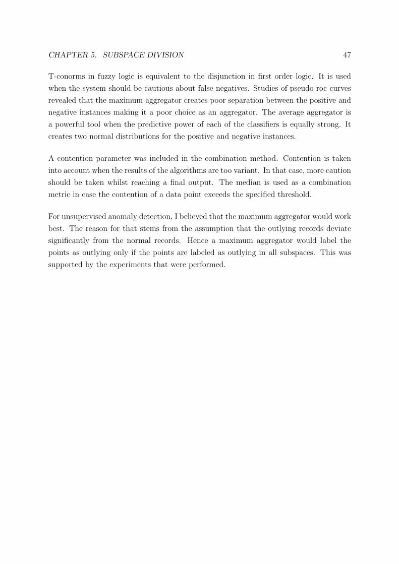
CHAPTER 5. SUBSPACE DIVISION 47
T-conorms in fuzzy logic is equivalent to the disjunction in first order logic. It is used
when the system should be cautious about false negatives. Studies of pseudo roc curves
revealed that the maximum aggregator creates poor separation between the positive and
negative instances making it a poor choice as an aggregator. The average aggregator is
a powerful tool when the predictive power of each of the classifiers is equally strong. It
creates two normal distributions for the positive and negative instances.
A contention parameter was included in the combination method. Contention is taken
into account when the results of the algorithms are too variant. In that case, more caution
should be taken whilst reaching a final output. The median is used as a combination
metric in case the contention of a data point exceeds the specified threshold.
For unsupervised anomaly detection, I believed that the maximum aggregator would work
best. The reason for that stems from the assumption that the outlying records deviate
significantly from the normal records. Hence a maximum aggregator would label the
points as outlying only if the points are labeled as outlying in all subspaces. This was
supported by the experiments that were performed.

Chapter 6
Experiments
6.1 Performance Criteria
The output of the anomaly detection algorithms is a continuous score which is propor-
tional to how outlying the points are. Evaluating such scores depends on the rank of
the outliers in the dataset. Two closely related performance criteria that are used in the
literature are the Receiver Operator Characteristic (ROC) and the Precision Recall (PR)
curves. A ROC curve is constructed by plotting the false positive rate against the true
positive rate, whilst a PR curve plots the recall against the precision. A PR curve can be
easily constructed from the data of a ROC curve [16]. This section will give an overview
on both criteria. For SVM based anomaly detection algorithms, the number of support
vectors gives an indication on the complexity of the model learnt and on the computation
time of the algorithms.
Table 6.1: Confusion Matrix
actual positive actual negative
predicted positive True positives (TP) false negatives (FN)predicted negative False Positives (FP) true negatives (TN)
The objective of the anomaly detection algorithm is to correctly identify the outliers
from the remaining normal points. Varying a threshold over the outlier score would label
48

CHAPTER 6. EXPERIMENTS 49
some points as outlying. Each threshold would yield a corresponding confusion matrix.
Each matrix has four entries as shown in Table 6.1. True positives (TP) corresponds to
the points that were correctly identified as outlying. Normal points that are incorrectly
labeled as outlying are called false negatives (FN). The second row correspond to the
points that were labeled as normal. Again, they can either be correctly or incorrectly
labeled referring to true negatives (TN) and false positives (FP) respectively. The metrics
used by the ROC curve are the true positive rate and the false positive rate. The earlier
represents the ratio of outlying points that were correctly classified, while the latter
correspond to the ratio of the normal points that were incorrectly classified as outlying.
PR curve plots the recall against the precision. The recall is equivalent to the true
positive rate. Precision shows the ratio of correctly predicted outliers to the total number
of predicted outliers. The calculations used for the metrics are shown in Equation 6.1.
True positive rate =TP
TP + FN
False positive rate =FP
FP + TN
Recall =TP
TP + FN
Precision =TP
TP + FP
(6.1)
Image removed due to missing copyright for online publication.
Please obtain image from the website stated in the caption.
Figure 6.1: Receiver Operator Characteristic (ROC) curve. Figure obtained from [2]
Figure 6.1 demonstrates the characteristics of the ROC curve. Ideally, all the outlying

CHAPTER 6. EXPERIMENTS 50
points would have an outlier score greater than the normal points. In that case the true
positive rate and false positive rate would be 1.0 and 0.0 respectively, yielding a ROC
curve passing through the perfect classification point (upper left corner). The resulting
area under the curve (AUC) would be equal to 1.0. The ROC curve of a completely
random algorithm is also shown the figure. A random algorithm would have an AUC of
0.5. Therefore the area under the ROC curve is a good indication on the performance
of the algorithm, where it can be interpreted as the probability that an outlying point
would be ranked higher than a normal point. However, attention should be paid when
using the AUC as an overall performance indicator as the different parts of the ROC
curve might have varied importance depending on the application [2].
Image removed due to missing copyright for online publication.
Please obtain image from the website stated in the caption.
Figure 6.2: Precision Recall (PR) curve. Figure obtained from [2]
An example PR curve is shown in figure 6.2. A perfect anomaly detection algorithm would
detect all outliers with perfect precision. This would correspond a recall and precision
of 1; a single point in the upper right corner. In contrast to the ROC curve, PR curves
are not strictly monotonic. This is due to the fact that varying the decision threshold
dynamically affect the denominator of the precision. A random algorithm would maintain
a low precision independent of the recall. The area under the curve (PR-AUC) can also
be used as a performance indicator.
Even though ROC and PR curves are closely related, together they can offer a more
comprehensive understanding of the performance of the algorithm. The ease of the in-
terpretation of the ROC curve gives it an edge over the PR curve [2]. However as noted
by Davis and Goadrich [16], the PR curve is more insightful particularly in imbalanced
datasets (similar to any dataset satisfying the unsupervised anomaly detection assump-
tion). For datasets having a majority of the negative class, an increase in the number of

CHAPTER 6. EXPERIMENTS 51
false positives would cause a limited change in the false positive rate as it will be masked
by the large number of negative instances. This would provide a highly optimistic ROC
curve.
6.2 Gamma Tuning
Gamma is the parameter that determines the spread of the Gaussian kernel. It is a
crucial parameter that affects the SVM training. It is typically adjusted in a supervised
setting using validation. It can also be adjusted by solving a fisher linear discriminate
model [58]. In an unsupervised setting this problem becomes more challenging due to
the absence of class labels. An approach suggested by [20] tries to automatically tune
gamma independent of the training process.
The kernel entries in an unsupervised setting represent the similarity between the dataset
points. It is desirable to have diverse entries in accordance to the fundamental premise
of pattern recognition:
(K(xi, xj)|(yi = yj)) > (K(xi, xj)|yi 6= yj) (6.2)
The values for the kernel entries for large γ approach zero, yielding an over-fitted decision
function. In the case where γ is too small, the kernel values approach 1, which yields a
poorly defined decision function. The objective is to maintain the majority of the entries
between 0.4 and 0.6.
1.0 0.4 · · · 0.6
0.4 1.0 · · · 0.3...
.... . .
...
0.6 0.5 · · · 1.0
This can be achieved by maximizing the following objective function:
s2
K + ε(6.3)

CHAPTER 6. EXPERIMENTS 52
K(xi, xj) = e−γ·‖xi−xj‖
K =
∑li=1
∑lj=i+1K(xi, xj)
l
s2 =
∑ni=1
∑nj=i+1 (K(xi, xj)− K)2
l − 1
where l is the number of non-diagonal entries, K and s correspond to the average and
the standard deviation of the non-diagonal entries of the kernel matrix.
The variance of the non-diagonal elements is always smaller than the its mean yielding a
global maximum for the optimization objective.
Gradient ascent is used in order to determine the optimal gamma value. The proper
initialization of gamma and the learning rate are crucial for fast convergence. The pa-
rameters were chosen dynamically according to the dataset to ensure ease of use.
The disadvantage of this approach is its time complexity. Each gradient ascent iteration
has a complexity of O(n2) forming a huge bottleneck in the performance of SVMs.
6.3 Datasets
Datasets from the UCI machine learning repository [22] are used for the evaluation of the
anomaly detection algorithms. Most of the datasets of UCI repository are traditionally
dedicated for classification tasks. Hence they have to be preprocessed in order to serve for
the evaluation of unsupervised anomaly detection algorithms. This is typically performed
by picking a meaningful outlying class and sampling the outliers to a small fraction [5].
Table 6.2 summarizes the characteristics of the preprocessed datasets.
The ionosphere dataset is composed of radar signals which are used to predict whether
there is a consistent structure in the ionosphere. The structure could either be good or
bad. The outlier class was chosen to be bad and 8 records were sampled using stratified
sampling to produce the processed dataset.

CHAPTER 6. EXPERIMENTS 53
Table 6.2: Summary of datasets information. Classes that are selected as outliers aredownsampled to satisfy the assumption of unsupervised anomaly detection.
Meta-data ionosphere shuttle breast-cancer satellite
Size 351 58000 569 6435Attributes 26 9 30 36Outlier Class(es) b 2 ,3 ,5 and 6 M 2,4 and 5Processed Dataset Size 233 46464 367 4486Outliers Percentage 3.4% 1.89% 2.72% 1.94%
The shuttle dataset is composed of various observations during the launching of space
shuttles. Similar to Reif et al [48], the outlier classes were chosen to be 2, 3, 5 and 6.
They were also sampled using stratified sampling, keeping only 878 outliers.
The features of breast-cancer represent the characteristics of breast masses. There are
two possible classification benign (B) and malignant (M). Intuitively the malignant class
should be the outlier class as the majority of the masses are benign. Only the first 10
malignant records were kept similar to [35].
The satellite dataset consists of 3x3 sections of a satellite multi-spectral image. The label
of each record represents the classification of the central pixel. Similar to [12], the three
smallest classes were chosen as the outlier class: 2, 4 and 5. Those classes were filtered
out except of 87 records that were chosen using stratified sampling.
The preprocessing was also performed using RapidMiner. For ionosphere, shuttle and
satellite, stratified sampling was used to reduce the number of outliers (for reproducibility,
the pseudo random generator seed was set to 1992).
6.4 Results
In this section, the performance of all the proposed one-class SVMs is compared against
the nine standard algorithms that were revised in Chapter 2. The experiments were
conducted using RapidMiner [39], where all of the algorithms are implemented in the

CHAPTER 6. EXPERIMENTS 54
Anomaly Detection extension1.
Table 6.3 shows ROC AUC results of the algorithms investigated. For a more complete
analysis, Figures 6.3 and 6.4 show the ROC curves and PR curves respectively. In each
figure, the three SVM based algorithms are plotted with the best algorithm in terms of
AUC from each category. The number of support vectors of the SVM based algorithms
are shown in table 6.4. The average CPU execution time of the algorithms over 10 runs
is shown in Table 6.5.
Table 6.3: Comparing the ROC AUC of SVM based algorithms against other anomalydetection algorithms
Dataset One-class Robust one-class Eta one-class k-NN LOF COF INFLO LoOP Histogram CBLOF u-CBLOF LDCOF
ionosphere 0.9878 0.9956 0.9972 0.9933 0.9178 0.9406 0.9406 0.9211 0.7489 0.3183 0.9822 0.9306shuttle 0.9936 0.9597 0.9941 0.9208 0.6072 0.5612 0.5303 0.5655 0.9889 0.8700 0.8739 0.5312breast-cancer 0.9843 0.9754 0.9833 0.9826 0.9916 0.9888 0.9922 0.9882 0.9829 0.8389 0.9743 0.9804satellite 0.8602 0.8861 0.8544 0.9003 0.8964 0.8708 0.8592 0.8664 0.8862 0.4105 0.9002 0.8657
In terms of AUC ROC, Table 6.3 shows that all SVM based algorithms perform generally
well on all datasets. For ionosphere and shuttle the eta one-class SVM is even superior.
For the breast-cancer dataset, SVM based algorithms score on average. For the satellite
dataset, where also many support vectors have been found, results are below the average.
Studying Figures 6.3 and 6.4 gives more insight into the results. Eta one-class SVM
performs best on the ionosphere dataset. It dominates in both, in the ROC and the PR
space (except for a small portion of PR space between the recall of [0.6, 0.7] where robust
one-class outperforms it), as shown in Figures 6.3a and 6.4a. It is also the best performing
algorithm for the shuttle dataset in the ROC space, as shown in Figure 6.3a. However, the
histogram approach clearly dominates in the PR space, shown in Figure 6.4b, followed
by robust one-class SVM. Figure 6.4d shows that eta one-class and u-CBLOF are the
dominating curves in the PR space of satellite dataset up until a recall of 0.3. In fact
they have perfect precision which means that 26 out of 87 outliers were ranked highest
by the algorithms. It is interesting to note that KNN the superior algorithm in the ROC
space performs very poorly in the PR space. The results of the breast-cancer dataset are
depicted in Figures 6.3c and 6.4c. Here, INFLO, which is a local density nearest-neighbor
based method, performs best. Examining the AUC results given in Table 6.3 shows that
the performance of SVM based algorithms on this dataset is comparable to k-NN. This
could possibly be an indicator that SVM based algorithms are error-prone in detecting
1Available athttp://code.google.com/p/rapidminer-anomalydetection/

CHAPTER 6. EXPERIMENTS 55
local outliers.
Tables 6.4 and 6.5 give room for further analysis of the performance of SVM based
algorithms. In general, the proposed SVM modifications, robust one-class and eta one-
class SVMs, produce a sparser solution. This has the advantage of avoiding over-fitting
and having a simple model. In addition, there is a possible improvement in the time
efficiency, which is especially apparent with large datasets, shuttle and satellite. The eta
one-class SVM is not efficient for small datasets due to the iterative nature of its solver.
Table 6.4: Number of support vectors of SVM based algorithms
Algorithm ionosphere shuttle breast-cancer satellite
One-class 106 21374 144 2085Robust One-class 116 5 90 385Eta One-class 37 8 48 158
Table 6.5: CPU execution time of SVM based algorithms
Algorithm ionosphere [ms] shuttle [s] breast-cancer [ms] satellite [s]
One-class 21.55± 0.26 747.15± 10.94 48.72± 1.01 14.02± 2.00Robust one-class 33.82± 0.26 218.93± 3.17 57.27± 2.29 8.60± 0.06Eta one-class 27.48± 0.25 4.07± 0.14 82.46± 0.42 12.35± 0.95

CHAPTER 6. EXPERIMENTS 56
0
0.2
0.4
0.6
0.8
1
0 0.2 0.4 0.6 0.8 1
Tru
e p
ositiv
e r
ate
False positive rate
Eta One-class,AUC=0.9972
Robust One-class,AUC=0.9956
k-NN,AUC=0.9933
One-class,AUC=0.9878
u-CBLOF,AUC=0.9822
Histogram,AUC=0.7489
(a) Ionosphere
0
0.2
0.4
0.6
0.8
1
0 0.1 0.2 0.3 0.4 0.5 0.6 0.7 0.8 0.9 1
Tru
e p
ositiv
e r
ate
False positive rate
Eta one-class,AUC=0.9941
One-class,AUC=0.9936
Histogram,AUC=0.9890
Robust one-class,AUC=0.9597
k-NN,AUC=0.9208
u-CBLOF,AUC=0.8739
(b) Shuttle
Figure 6.3: ROC curves for SVM based algorithms and existing approaches. For thelatter, the best performing algorithms of the categories nearest-neighbor, statistical andclustering based are plotted

CHAPTER 6. EXPERIMENTS 57
0
0.2
0.4
0.6
0.8
1
0 0.2 0.4 0.6 0.8 1
Tru
e p
ositiv
e r
ate
False positive rate
INFLO,AUC=0.9921
One-class,AUC=0.9843
Eta One-class,AUC=0.9833
Histogram,AUC=0.9830
LDCOF,AUC=0.98032
Robust One-class,AUC=0.9754
(c) Breast Cancer
0
0.2
0.4
0.6
0.8
1
0 0.2 0.4 0.6 0.8 1
Tru
e p
ositiv
e r
ate
False positive rate
k-NN,AUC=0.9003
u-CBLOF,AUC=0.9002
Histogram,AUC=0.8862
Robust one-class,AUC=0.8861
One-class,AUC=0.8602
Eta one-class,AUC=0.8544
(d) Satellite
Figure 6.3: ROC curves for SVM based algorithms and existing approaches. For thelatter, the best performing algorithms of the categories nearest-neighbor, statistical andclustering based are plotted

CHAPTER 6. EXPERIMENTS 58
0
0.2
0.4
0.6
0.8
1
0 0.2 0.4 0.6 0.8 1
Pre
cis
ion
Recall
One-class
Eta One-class
Robust One-class
k-NN
u-CBLOF
Histogram
(a) Ionosphere
0
0.2
0.4
0.6
0.8
1
0 0.2 0.4 0.6 0.8 1
Pre
cis
ion
Recall
One-class
Robust one-class
Eta one-class
k-NN
u-CBLOF
Histogram
(b) Shuttle
Figure 6.4: PR curves

CHAPTER 6. EXPERIMENTS 59
0
0.2
0.4
0.6
0.8
1
0 0.2 0.4 0.6 0.8 1
Pre
cis
ion
Recall
One-class
Robust One-class
Eta One-class
INFLO
LDCOF
Histogram
(c) Breast Cancer
0
0.2
0.4
0.6
0.8
1
0 0.1 0.2 0.3 0.4 0.5 0.6 0.7 0.8 0.9 1
Pre
cis
ion
Recall
One-class
Robust one-class
Eta one-class
k-NN
u-CBLOF
Histogram
(d) Satellite
Figure 6.4: PR curves

CHAPTER 6. EXPERIMENTS 60
6.5 Subspace Division
The technique proposed by Evangelista [18] has never been investigated in an unsuper-
vised setting. There are several questions that need to be addressed in order to better
understand the approach in our context:
• Does subspace division produce an improvement in the performance over the tra-
ditional application of the algorithm?
• Is intelligent subspace modeling necessary for the effectiveness of the technique?
• Are the results of genetic algorithms relatively stable over different runs?
In the following subsections, the suggested questions are briefly investigated using the
satellite dataset. This dataset was used for investigating subspace division as it has 36
attributes. Also, it is a large dataset, with 87 outliers, and the best AUC obtained for
SVM based algorithms was 0.8861, which leaves a significant room for improvement.
To answer the first question, the performance of the SVM based algorithms is compared
with and without subspace division. Figure 6.5 shows the corresponding ROC curves.
The number of subspaces used by the division algorithms were 4. Introducing subspaces
improved the performance of one-class and eta one-class SVM, where the first showed a
trivial improvement in the AUC ROC by 0.002 and eta one-class SVM produced a better
improvement by 0.01 .
Verifying the importance of intelligent subspace selection is crucial to justify the added
computational complexity. Two other division methods were investigated in addition to
PCA and Kendall division as described in Section 5.3: Subspace Outlier Ensemble using
1-dimensional subspaces (SOE1) and a dataset dependent division. SOE1 was suggested
in [27] as a simple division method to verify the effectiveness of subspace division for
outlier detection. As its name implies it uses subspaces containing only 1 dimension. The
last division method, which is a dataset dependent division, uses some porperties of the
dataset to create meaningful subspaces. The satellite dataset describes a multi-spectral
image and hence a possible division is on a channel basis yielding 4 subspaces. This
method was included to verify that not just any division would improve the results.
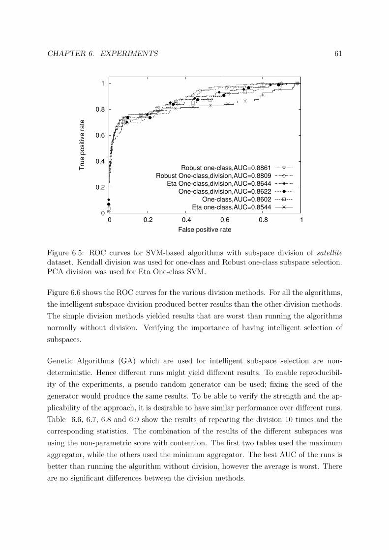
CHAPTER 6. EXPERIMENTS 61
0
0.2
0.4
0.6
0.8
1
0 0.2 0.4 0.6 0.8 1
Tru
e p
ositiv
e r
ate
False positive rate
Robust one-class,AUC=0.8861
Robust One-class,division,AUC=0.8809
Eta One-class,division,AUC=0.8644
One-class,division,AUC=0.8622
One-class,AUC=0.8602
Eta one-class,AUC=0.8544
Figure 6.5: ROC curves for SVM-based algorithms with subspace division of satellitedataset. Kendall division was used for one-class and Robust one-class subspace selection.PCA division was used for Eta One-class SVM.
Figure 6.6 shows the ROC curves for the various division methods. For all the algorithms,
the intelligent subspace division produced better results than the other division methods.
The simple division methods yielded results that are worst than running the algorithms
normally without division. Verifying the importance of having intelligent selection of
subspaces.
Genetic Algorithms (GA) which are used for intelligent subspace selection are non-
deterministic. Hence different runs might yield different results. To enable reproducibil-
ity of the experiments, a pseudo random generator can be used; fixing the seed of the
generator would produce the same results. To be able to verify the strength and the ap-
plicability of the approach, it is desirable to have similar performance over different runs.
Table 6.6, 6.7, 6.8 and 6.9 show the results of repeating the division 10 times and the
corresponding statistics. The combination of the results of the different subspaces was
using the non-parametric score with contention. The first two tables used the maximum
aggregator, while the others used the minimum aggregator. The best AUC of the runs is
better than running the algorithm without division, however the average is worst. There
are no significant differences between the division methods.

CHAPTER 6. EXPERIMENTS 62
Table 6.6: Results of PCA division with maximum aggregator.
Algorithm 36 var Average range r-coefficient
One-class 0.8602 0.8605±0.0081 [0.8474;0.8793] -0.4953Robust One-class 0.8861 0.8793±0.0082 [0.8613;0.8980] -0.4482Eta-one-class 0.8544 0.8520±0.0112 [0.8313;0.8787] -0.3466
Table 6.7: Results of Kendall division with maximum aggregator.
Algorithm 36 var Average range r-coefficient
One-class 0.8602 0.8606±0.0059 [0.8438;0.8704] 0.3159Robust One-class 0.8861 0.8762±0.0057 [0.8625;0.8902] 0.1847Eta-one-class 0.8544 0.8531±0.0077 [0.8363;0.8676] 0.0625
Table 6.8: Results of PCA division with minimum aggregator
Algorithm 36 var Average range r-coefficient
One-class 0.8602 0.8618±0.0105 [0.8434;0.8874] -0.3210Robust One-class 0.8861 0.8790±0.0070 [0.8631;0.8906] -0.3588Eta-one-class 0.8544 0.8465±0.0139 [0.8156;0.8821] -0.2708
Table 6.9: Results of Kendall division with minimum aggregator.
Algorithm 36 var Average range r-coefficient
One-class 0.8602 0.8617±0.0078 [0.8437;0.8769] 0.2351Robust One-class 0.8861 0.8789±0.0046 [0.8698;0.8883] -0.2665Eta-one-class 0.8544 0.8524±0.0127 [0.8215;0.8756] 0.3326
Both of the division methods are based on the premise that the more independent sub-
spaces are superior in outlier detection. Thus in theory, if the GA ran for infinite evo-
lutions it would reach the fittest division and hence the best solution. So to verify the
premise, the Pearson r-coefficient between the fitness of the division and the resulting
AUC was calculated that should unfold any linear correlation. The premise should result
in a r-coefficient approximately equal to -1 (smaller fitness indicates a more indepen-
dent solution). The PCA division yielded a better coefficient as it had the correct sign.
However, all the correlations are weak as there magnitude is less that 0.5.

CHAPTER 6. EXPERIMENTS 63
0
0.2
0.4
0.6
0.8
1
0 0.2 0.4 0.6 0.8 1
Tru
e p
ositiv
e r
ate
False positive rate
Kendall,AUC=0.8623
36 var,AUC=0.8602
PCA,AUC=0.8595
Channels,AUC=0.7361
1D subspaces,AUC=0.6358
(a) One-class SVM
0
0.2
0.4
0.6
0.8
1
0 0.2 0.4 0.6 0.8 1
Tru
e p
ositiv
e r
ate
False positive rate
36 var,AUC= 0.8861
Kendall,AUC=0.8809
PCA,AUC= 0.8736
1D subspaces,AUC=0.8352
Channels,AUC=0.8284
(b) Robust One-class SVM
Figure 6.6: ROC Curves for different subspace division methods

CHAPTER 6. EXPERIMENTS 64
0
0.2
0.4
0.6
0.8
1
0 0.2 0.4 0.6 0.8 1
Tru
e p
ositiv
e r
ate
False positive rate
PCA,AUC= 0.8644
Kendall,AUC=0.8394
36 var,AUC=0.8544
Channels,AUC=0.7433
1D subspaces,AUC=0.1464
(c) Eta One-class SVM
Figure 6.6: ROC Curves for different subspace division methods

CHAPTER 6. EXPERIMENTS 65
6.6 Gamma Values
In an unsupervised setting, the task of parameter selection becomes increasingly diffi-
cult. In the experiments, the parameter tuning method described earlier in Section 6.2.
The method resulted in the γ values as shown in Table 6.10. As the parameter tuning
algorithm is quiet expensive, this section is dedicated to showing its importance.
Table 6.10: Tuned γ values
Data Set γ
ionosphere 9.182 · 10−1
shuttle 2.627 · 10−6
breast-cancer 3.655 · 10−4
satellite 5.170 · 10−4
Figure 6.7 shows the result of varying gamma on the ROC AUC value. For all datasets,
the tuned gamma produces very good results for the three algorithms. The importance
of the gamma selection is especially evident in the ionosphere dataset shown in Fig-
ure 6.7a, where the parameter tuning algorithm managed to select the best gamma for
both: one-class SVM and robust one-class SVM.

CHAPTER 6. EXPERIMENTS 66
0.5
0.6
0.7
0.8
0.9
1
0 0.2 0.4 0.6 0.8 1 1.2 1.4 1.6 1.8 2
RO
C A
UC
γ
One-class
Robust
Eta
(a) Ionosphere
0.5
0.6
0.7
0.8
0.9
1
0 0.1 0.2 0.3 0.4 0.5 0.6 0.7 0.8 0.9 1
RO
C A
UC
γ.10-3
One-class
Robust
Eta
(b) Breast Cancer
Figure 6.7: Plotting the result of varying γ on AUC. The vertical line represents thetuned γ value

CHAPTER 6. EXPERIMENTS 67
0.5
0.6
0.7
0.8
0.9
1
0 0.1 0.2 0.3 0.4 0.5 0.6 0.7 0.8 0.9 1
RO
C A
UC
γ.10-3
One-class
Robust
Eta
(c) Satellite
Figure 6.7: Plotting the result of varying γ on AUC. The vertical line represents thetuned γ value

Chapter 7
Conclusion
The experiments demonstrated the competence of SVM based algorithms, in detecting
outliers, in an unsupervised anomaly detection setting. According to the ROC AUC,
which is the most popular evaluation criteria for anomaly detection, SVM based algo-
rithms are even superior on two out the four datasets. The strong theoretical foundation
of SVMs enabled it to perform reasonably well on all the datasets. Even for the satellite
dataset, where the SVM based algorithms were outperformed in terms of the ROC AUC
by the algorithms in the other existing categories, the proposed eta one-class SVM was
clearly a very good candidate for detecting the top outliers, shown by its dominance in
the PR space.
The eta one-class SVM has shown the greatest potential among the one-class SVM for-
mulations. It is capable of maintaining the sparsity of the SVM solution, whilst perform-
ing best on most datasets. Concerning the second proposed enhancement, the robust
one-class SVM produced a more sparse solution than one-class SVM, however in terms
of the performance, the off-the-shelf one-class SVM is still superior.
Applying the subspace modeling approach for SVM based algorithms in an unsupervised
setting has shown no improvement in the results. The methods investigated for selecting
subspaces were non-deterministic and on average they performed worse than the algo-
rithms applied on the full input space. There are couple of reasons that might have
contributed to the disappointing results. First, it has been argued that SVMs are already
robust against the curse of dimensionality [58]. In light of that argument, the approach
68

CHAPTER 7. CONCLUSION 69
might work using other unsupervised anomaly detection algorithms; you can not fix what
was not broken. Second, several researchers have questioned the applicability of the ROC
as an evaluation metric in highly skewed data [16]. Thus, an alternative performance cri-
teria might be able to better judge the effectiveness of the approach. Also, having several
subspaces makes the parameter selection an impossible task. Whilst the gamma was au-
tomatically tuned with and without division, other critical parameters, such as the ν for
one-class SVM, were selected for the normal application of the algorithms using a quick
grid search, which is inapplicable with the increasing number of subspaces. It should also
be noted that the evaluation included only one dataset, which is definitely not enough to
omit the approach altogether.
One of the major advantages of SVMs is its time complexity, attributed to the sparsity
property. Unfortunately, the tuning of gamma for the Gaussian kernel similar to [20],
has a quadratic time complexity, which forms a major bottleneck in the performance of
SVMs.
The breadth of the presented work opens several directions for future research. The first
direction is regarding SVMs for unsupervised anomaly detection. The Gaussian kernel is
only one example of the wide class of kernels called Radial Basis Function (RBF) kernels.
Some of those kernels might be better suited for the problem at hand, thus it is worth
investigating. Also, further analysis of the critical parameters of the proposed methods,
λ for robust one-class SVM and β for eta one-class SVM, is essential in order to provide a
foundation as strong as that provided by the classical one-class SVM. Regarding subspace
division, it will be interesting to see the results of the approach using other unsupervised
anomaly detection algorithms. In general, more experiments need to be implemented,
using both real and synthetic datasets, to support the reached outcomes.
To conclude, SVM based algorithms have exhibited great potential for unsupervised
anomaly detection. In particular, the eta one-class SVM is a very attractive choice for
investigation when applying unsupervised anomaly detection in practice.

Bibliography
[1] Charu C. Aggarwal. Outlier ensembles: position paper. SIGKDD Explorations,
14(2):49–58, 2012.
[2] Charu C. Aggarwal. Outlier Analysis. Springer New York, New York, NY, 2013.
[3] Rakesh Agrawal and Ramakrishnan Srikant. Mining sequential patterns. In Proceed-
ings of the 11th International Conference on Data Engineering, pages 3–14. IEEE
Computer Society, Washington, DC, USA, 1995.
[4] Jess S. Aguilar-Ruiz, Roberto Ruiz, Jos Cristbal Riquelme Santos, and Ral Girldez.
Snn: A supervised clustering algorithm. In Laszlo Monostori, Jzsef Vncza, and
Moonis Ali, editors, IEA/AIE, volume 2070 of Lecture Notes in Computer Science,
pages 207–216. Springer, 2001.
[5] Mennatallah Amer and Markus Goldstein. Nearest-Neighbor and Clustering based
Anomaly Detection Algorithms for RapidMiner. Proc. of the 3rd RapidMiner Com-
munity Meeting and Conference (RCOMM 2012), pages 1–12, 2012.
[6] Mennatallah Amer, Markus Goldstein, and Slim Abdennadher. Enhancing One-class
Support Vector Machines for Unsupervised Anomaly Detection. Proceeding of the
19th ACM SIGKDD Conference, 2013.
[7] Fabrizio Angiulli and Clara Pizzuti. Fast outlier detection in high dimensional spaces.
In Tapio Elomaa, Heikki Mannila, and Hannu Toivonen, editors, Principles of Data
Mining and Knowledge Discovery, volume 2431 of Lecture Notes in Computer Sci-
ence, pages 43–78. Springer Berlin / Heidelberg, 2002.
70

BIBLIOGRAPHY 71
[8] Christopher M. Bishop. Pattern Recognition and Machine Learning (Information
Science and Statistics). Springer, 1st ed. 2006. corr. 2nd printing 2011 edition,
October 2007.
[9] Markus M. Breunig, Hans-Peter Kriegel, Raymond T. Ng, and Jorg Sander. LOF:
Identifying Density-Based Local Outliers. In Proc. of the 2000 ACM SIGMOD Int.
Conf. on Management of Data, pages 93–104, Dallas, Texas, USA, 05 2000. ACM.
[10] Christopher J. C. Burges. A tutorial on support vector machines for pattern recog-
nition. Data Mining and Knowledge Discovery, 2:121–167, 1998.
[11] W. M. Campbell, J. P. Campbell, D. A. Reynolds, D. A. Jones, and T. R. Leek.
Phonetic speaker recognition with support vector machines. In in Advances in Neural
Information Processing Systems, pages 1377–1384. MIT Press, 2004.
[12] Uriel Carrasquilla. Benchmarking algorithms for detecting anomalies in large
datasets. MeasureIT, Nov, 2010.
[13] Varun Chandola, Arindam Banerjee, and Vipin Kumar. Anomaly detection: A
survey. ACM Comput. Surv., 41(3):15:1–15:58, July 2009.
[14] Chih-Chung Chang and Chih-Jen Lin. Libsvm: A library for support vector ma-
chines. ACM Trans. Intell. Syst. Technol., 2(3):27:1–27:27, May 2011.
[15] Nello Cristianini and John Shawe-Taylor. An Introduction to Support Vector Ma-
chines and Other Kernel-based Learning Methods. Cambridge University Press, 1
edition, 2000.
[16] Jesse Davis and Mark Goadrich. The relationship between Precision-Recall and ROC
curves. Proceedings of the 23rd international conference, 2006.
[17] Martin Ester, Hans peter Kriegel, Jrg S, and Xiaowei Xu. A density-based algorithm
for discovering clusters in large spatial databases with noise. pages 226–231. AAAI
Press, 1996.
[18] Paul F. Evangelista. The unbalanced classification problem: detecting breaches in
security. PhD thesis, Rensselaer Polytechnic Institute, 2006.
[19] Paul F. Evangelista, Piero Bonnisone, Mark J. Embrechts, and Boleslaw K. Szy-
manski. FUZZY ROC CURVES FOR THE 1 CLASS SVM : APPLICATION TO
INTRUSION DETECTION, 2005.

BIBLIOGRAPHY 72
[20] Paul F. Evangelista, Mark J. Embrechts, and Boleslaw K. Szymanski. Some proper-
ties of the gaussian kernel for one class learning. In Proc. of the 17th Int. Conf. on
Artificial neural networks, ICANN’07, pages 269–278. Springer Berlin / Heidelberg,
2007.
[21] Rong-En Fan, Pai-Hsuen Chen, and Chih-Jen Lin. Working set selection using
second order information for training support vector machines. J. Mach. Learn.
Res., 6:1889–1918, December 2005.
[22] A. Frank and A. Asuncion. UCI machine learning repository, 2010.
[23] Markus Goldstein and Andreas Dengel. Histogram-based outlier score (hbos): A
fast unsupervised anomaly detection algorithm. In Stefan Wolfl, editor, KI-2012:
Poster and Demo Track, pages 59–63. Online, 9 2012.
[24] Sudipto Guha, Rajeev Rastogi, and Kyuseok Shim. Rock: A robust clustering
algorithm for categorical attributes. In Masaru Kitsuregawa, Michael P. Papazoglou,
and Calton Pu, editors, ICDE, pages 512–521. IEEE Computer Society, 1999.
[25] Simon Hawkins, Hongxing He, Graham Williams, and Rohan Baxter. Outlier detec-
tion using replicator neural networks. In In Proc. of the Fifth Int. Conf. and Data
Warehousing and Knowledge Discovery (DaWaK02, pages 170–180, 2002.
[26] Zengyou He, Xiaofei Xu, and Shengchun Deng. Discovering cluster-based local out-
liers. Pattern Recognition Letters, 24(9-10):1641–1650, 2003.
[27] Zengyou He, Xiaofei Xu, and Shengchun Deng. A unified subspace outlier ensemble
framework for outlier detection in high dimensional spaces. CoRR, abs/cs/0505060,
2005.
[28] Ralf Herbrich and Jason Weston. Adaptive margin support vector machines for
classification. In ADVANCES IN LARGE MARGIN CLASSIFIERS, pages 281–
295. MIT Press, 2000.
[29] Harold Hotelling. Relations Between Two Sets of Variates. Biometrika, 28(3/4):321–
377, December 1936.
[30] Wenjie Hu, Yihua Liao, and V. Rao Vemuri. Robust anomaly detection using support
vector machines. In In Proceedings of the International Conference on Machine
Learning. Morgan Kaufmann Publishers Inc, 2003.

BIBLIOGRAPHY 73
[31] W.J. Hu and Q. Song. An accelerated decomposition algorithm for robust support
vector machines. Circuits and Systems II: Express Briefs, IEEE Transactions on,
51(5):234–240, 2004.
[32] Wen Jin, Anthony Tung, Jiawei Han, and Wei Wang. Ranking outliers using sym-
metric neighborhood relationship. In Wee-Keong Ng and et al., editors, Advances in
Knowledge Discovery and Data Mining, volume 3918 of Lecture Notes in Computer
Science, pages 577–593. Springer Berlin / Heidelberg, 2006.
[33] Maurice G. Kendall. Rank correlation methods. Griffin, London, 1948.
[34] Nir Krause and Yoram Singer. Leveraging the margin more carefully. In In Inter-
national Conference on Machine Learning, ICML, 2004.
[35] Hans-Peter Kriegel, Peer Kroger, Erich Schubert, and Arthur Zimek. Loop: local
outlier probabilities. In Proceeding of the 18th ACM Conf. on Information and
knowledge management, CIKM ’09, pages 1649–1652, New York, NY, USA, 2009.
ACM.
[36] Pavel Laskov, Christin Schafer, Igor V. Kotenko, and Klaus-Robert Muller. Intrusion
detection in unlabeled data with quarter-sphere support vector machines. Praxis der
Informationsverarbeitung und Kommunikation, 27(4):228–236, 2007.
[37] Jessica Lin, Eamonn Keogh, Ada Fu, and Helga Van Herle. Approximations to magic:
Finding unusual medical time series. In In 18th IEEE Symp. on Computer-Based
Medical Systems (CBMS, pages 23–24, 2005.
[38] Yi Liu and Yuan F. Zheng. Minimum enclosing and maximum excluding machine
for pattern description and discrimination. Pattern Recognition, International Con-
ference on, 3:129–132, 2006.
[39] I. Mierswa, M. Wurst, R. Klinkenberg, M. Scholz, and T. Euler. Yale (now: Rapid-
miner): Rapid prototyping for complex data mining tasks. In Proc. of the ACM
SIGKDD Int. Conf. on Knowledge Discovery and Data Mining (KDD 2006), 2006.
[40] S. Mukkamala, G. Janoski, and A. Sung. Intrusion detection using neural networks
and support vector machines. Proc. of the 2002 Int. Joint Conf. on Neural Networks.
IJCNN’02 (Cat. No.02CH37290), pages 1702–1707, 2002.

BIBLIOGRAPHY 74
[41] Edgar Osuna, Robert Freund, and Federico Girosi. An improved training algorithm
for support vector machines. In Neural Networks for Signal Processing [1997] VII.
Proceedings of the 1997 IEEE Workshop, pages 276–285, 1997.
[42] Gregory Piatetsky. Kdnuggets annual software poll, June 2013.
[43] John C. Platt. Advances in kernel methods. chapter Fast training of support vector
machines using sequential minimal optimization, pages 185–208. MIT Press, Cam-
bridge, MA, USA, 1999.
[44] M. Pontil and A. Verri. Support vector machines for 3d object recognition. Pattern
Analysis and Machine Intelligence, IEEE Transactions on, 20(6):637–646, 1998.
[45] Leonid Portnoy, Eleazar Eskin, and Sal Stolfo. Intrusion detection with unlabeled
data using clustering. In In Proc. of ACM CSS Workshop on Data Mining Applied
to Security (DMSA-2001), pages 5–8, 2001.
[46] Amar S Kapoor Rakesh Kaundal and Gajendra PS Raghava. Machine learning
techniques in disease forecasting: a case study on rice blast prediction. BMC Bioin-
formatics, 2006.
[47] Sridhar Ramaswamy, Rajeev Rastogi, and Kyuseok Shim. Efficient algorithms for
mining outliers from large data sets. In Proc. of the 2000 ACM SIGMOD Int. Conf.
on Management of Data, SIGMOD ’00, pages 427–438, New York, NY, USA, 2000.
ACM.
[48] Matthias Reif, Markus Goldstein, Armin Stahl, and Thomas M. Breuel. Anomaly
detection by combining decision trees and parametric densities. 2008 19th Interna-
tional Conference on Pattern Recognition, pages 1–4, December 2008.
[49] Bernhard Scholkopf, John C Platt, John Shawe-Taylor, Alex J Smola, and Robert C
Williamson. Estimating the support of a high-dimensional distribution. Neural
computation, 13(7):1443–71, July 2001.
[50] Bernhard Scholkopf, Robert C. Williamson, Alex J. Smola, John Shawe-Taylor, and
John C. Platt. Support vector method for novelty detection. In Advances in Neural
Information Processing Systems 12, (NIPS) Conf., pages 582–588. The MIT Press,
11 1999.

BIBLIOGRAPHY 75
[51] Qing Song, Wenjie Hu, and Wenfang Xie. Robust support vector machine with bullet
hole image classification. Systems, Man and Cybernetics, Part C, IEEE Transactions
on, 32(4):440–448, 2002.
[52] Kyoko Sudo, Tatsuya Osawa, Kaoru Wakabayashi, and Hideki Koike. Detecting the
degree of anomaly in security video. IAPR Conference on Machine Vision Applica-
tion, pages 53–56, 2007.
[53] Jian Tang, Zhixiang Chen, Ada Fu, and David Cheung. Enhancing effectiveness of
outlier detections for low density patterns. In Ming-Syan Chen, Philip Yu, and Bing
Liu, editors, Advances in Knowledge Discovery and Data Mining, volume 2336 of
Lecture Notes in Computer Science, pages 535–548. Springer Berlin / Heidelberg,
2002.
[54] David M. J. Tax and Robert P. W. Duin. Support vector domain description. Pattern
Recognition Letters, 20:1191–1199, 1999.
[55] Joost van Beusekom and Faisal Shafait. Distortion measurement for automatic doc-
ument verification. In Proc. of the 11th Int. Conf. on Document Analysis and Recog-
nition. IEEE, 9 2011.
[56] V. Vapnik. Statistical learning theory. Wiley, 1 edition, September 1998.
[57] V. Vapnik and A. Lerner. Pattern recognition using generalized portrait method.
Automation and Remote Control, 24:774–780, 1963.
[58] Wenjian Wang, Zongben Xu, Weizhen Lu, and Xiaoyun Zhang. Determination of
the Spread Parameter in the Gaussian Kernel for Classification and Regression.
Neurocomputing, 55(3-4):643–663, October 2003.
[59] Yichao Wu and Yufeng Liu. Robust truncated-hinge-loss support vector machines.
JASA, 2007.
[60] Linli Xu, K Crammer, and Dale Schuurmans. Robust support vector machine train-
ing via convex outlier ablation. Proc. of the National Conf. On Artificial Intelligence,
pages 536–542, 2006.
[61] Alan Yuille and Anand Rangarajan. The concave-convex procedure (CCCP). In
Advances in Neural Information Processing Systems 14. MIT Press, 2002.

BIBLIOGRAPHY 76
[62] Tong Zhang. Analysis of multi-stage convex relaxation for sparse regularization. J.
Mach. Learn. Res., 11:1081–1107, March 2010.
[63] Xi-chuan Zhou, Hai-bin Shen, and Jie-ping Ye. Integrating outlier filtering in large
margin training. Journal of Zhejiang University-Science C, 12(5):362–370, May 2011.