Embed Size (px)
Citation preview
ENERGY BALANCE OF MICROALGAE
BIOFUELS
Annika Weiss

This work is licensed under a Creative Commons Attribution-NonCommercial-NoDerivatives 4.0
International License.
ENERGY BALANCE OF MICROALGAE BIOFUELS
von Dipl.-Ing. Annika Weiss
Geboren in Ulm
Vom Fachbereich Bau- und Umweltingenieurwissenschaften der Technischen Universität Darmstadt zur Erlangung des akademischen Grades Doktorin der Ingenieurwissenschaften (Dr.-Ing.) genehmigte Dissertation
Darmstadt 2016
D17
Referentin: Prof. Dr. rer. nat. Liselotte Schebek, TU Darmstadt Korreferent: Prof. Dr.-Ing. Peter Cornel, TU Darmstadt
Tag der Einreichung: 25.11.2015 Tag der mündlichen Prüfung: 19.02.2016

i
Abstract
Microalgae are small organisms that live in the water and use solar energy to grow. Like plants, they can be used to produce biofuels. Since the Second World War there have been repeated attempts to produce biofuels from microalgae. The idea has recently received a boost due to one specific feature of microalgae: unlike other biofuel feedstock, microalgae do not compete with food production for arable land.
Biofuel production with microalgae is only sensible when less energy is required to produce the fuel than is stored in the fuel. The ratio of energy demand to energy output, the ‘Net Energy Ratio’ (NER), should be smaller than one. Previous studies have shown that the NER depends significantly on (a) the assumed operation energy, and (b) the expected biomass productivities. Although it is well-known that these two parameters are inherently linked, this dependency has not been considered when calculating the NER.
In this dissertation, for the first time biomass productivity is calculated based on operation energy. For this purpose, a correlation between the key parameters to model operation energy and biomass productivity (aeration rate, light intensity and photosynthetic efficiency (PE)) is derived and validated based on a systematic analysis of published experimental data. Based on this correlation, the NER of microalgae biofuels production is calculated. Aerated flat plate photobioreactors are investigated as a method of microalgae cultivation. These have previously been examined as promising systems for outdoor cultivation. As a biofuel, biomethane production is investigated since its production requires the least energy compared to other biofuels.
The results of this dissertation show that operation energy and biomass productivities are related non-linearly: to achieve high productivities, disproportionately more energy is required than to achieve low productivities. Consequently, the aim of energy-efficient microalgae cultivation is not to achieve the highest possible biomass yield but to find a good balance between operation energy and biomass yield. Furthermore, due to these interactions, the lowest possible NER is not achieved with the maximum biomass yield. The optimum NER depends on the interaction of all model parameters. The effect of parameter changes on the NER depends also on the aeration rate.
The NER calculated in this dissertation for aerated flat plate photobioreactors is around 1.8. This value is achieved at an aeration rate of 0.25 vvm (gas volume gas per liquid volume and minute). This corresponds, when coupled with the further findings and assumptions of this study, to an operation power of 54 W m-3 or 2.2 W m-2 and a biomass productivity of 50 t ha-1 y-1. A NER below one could not be achieved even though expected technological improvement is considered in the calculation. The calculated NER is compared to the NER results in previous studies which were partially below one. The analysis of previous studies showed that there are two main reasons for a NER < 1: one is incomplete system boundaries; the other is that the relation between energy demand and productivity is not considered.
With the systematic approach presented in this dissertation, the potential development of microalgae biofuel production can be predicted more reliably. Expected technological

ii
development could improve the relation between operation energy and biomass productivities, but it cannot uncouple these parameters. Their correlation is based on the fundamental principles of microalgae growth, which apply to all cultivation systems and all types of algae.
The method developed in this thesis can also be applied to quantify the best possible NER for other cultivation systems, based on the relation between operation energy and biomass productivity. The approach to correlating important model parameters based on the underlying scientific mechanisms can be transferred to other systems as well. It can thus also be applied to estimate the potential development of other technologies.

iii
Zusammenfassung
Mikroalgen sind im Wasser lebende Mikroorganismen, die mit Hilfe von Sonnenlicht wachsen. Bereits seit dem Zweiten Weltkrieg wird versucht, aus Algen Biotreibstoff herzustellen. Dieser Ansatz wird derzeit wieder verstärkt diskutiert, da Mikroalgen – im Gegensatz zu Landpflanzen – nicht mit Nahrungsmittelproduktion um fruchtbaren Boden konkurrieren.
Sinnvoll ist die Gewinnung von Biotreibstoff aus Mikroalgen nur dann, wenn weniger Energie benötigt wird, um den Treibstoff zu produzieren, als im gewonnenen Treibstoff gespeichert ist: Der Quotient dieser beiden Werte (Energieaufwand und Energiegehalt des Treibstoffes), der ‚Net Energy Ratio‘ (NER) muss kleiner eins sein. Bisherige Studien zeigen, dass im Wesentlichen zwei Parameter den NER bestimmen: Kultivierungsenergie und Biomasse-Ertrag. Obwohl diese beiden Parameter offensichtlich voneinander abhängen, wurde diese Abhängigkeit bisher nicht berücksichtigt, um den NER zu berechnen.
In dieser Dissertation wird erstmalig der Biomasse-Ertrag abhängig von der Kultivierungsenergie modelliert. Dazu wird eine Korrelation zwischen wichtigen Modellparametern (Begasungsrate, Lichtintensität und photosynthetischer Effizient (PE)) aus Experimentaldaten hergeleitet und anhand weiterer Literatur validiert. Diese Korrelation wird zugrunde gelegt, um den NER der Biotreibstoffproduktion aus Mikroalgen zu berechnen. Als Methode der Algenkultivierung werden begaste flache Photobioreaktoren untersucht. Diese wurden bisher als vielversprechende Systeme für die Freilandkultivierung intensiv erforscht. Als gewonnener Treibstoff wird beispielhaft Biomethan untersucht, da seine Produktion den geringsten Energiebedarf im Vergleich zur Produktion anderer Treibstoffe aufweist.
Die Ergebnisse dieser Arbeit zeigen, dass Kultivierungsenergie und Biomasse-Ertrag nichtlinear voneinander abhängen: um hohe Erträge zu erzielen, wird überproportional mehr Energie benötigt, als für niedrige Erträge. Um Mikroalgen möglichst energie-effizient zu kultivieren, sollte daher nicht der höchstmögliche Biomasse-Ertrag angestrebt werden, sondern vielmehr ein ausgewogenes Verhältnis zwischen Energiebedarf und Biomasse-Ertrag. Aus diesem Zusammenhang folgt weiterhin, dass ein niedriger NER nicht mit dem höchstmöglichen Biomasse-Ertrag zu erreichen ist. Der bestmögliche NER hängt von weiteren Modellparametern ab, die sich wechselseitig beeinflussen. Parameteränderungen wirken sich je nach Begasungsrate unterschiedlich stark auf den NER aus.
Der in der vorliegenden Arbeit berechnete NER für begaste Photobioreaktoren liegt bei etwa 1,8. Dieser Wert wird bei einer Begasungsrate von 0,25 vvm (Gasvolumen per Flüssigkeitsvolumen und Minute) erreicht. Das entspricht, zusammen mit den weiteren Ergebnissen und Annahmen und dieser Arbeit, einem Leistungseintrag von 54 W m-3 oder 2,2 W m-2 und einem Biomasse-Ertrag von 50 t ha-1 y-1. Ein NER unter eins kann nicht erreicht werden, obwohl zu erwartende Technologieentwicklung in die Berechnung miteinbezogen wurde.
iv
Der berechnete NER wird mit anderen Studien verglichen, die teilweise auf deutlich niedrigere NER kommen. Eine Analyse dieser Studien zeigt zwei Ursachen für einen NER < 1: Einerseits sind die Systemgrenzen zum Teil unvollständig, anderseits wird der Zusammenhang zwischen Energiebedarf und Biomasse-Ertrag nicht berücksichtigt.
Mit dem hier vorgestellten systematischen Ansatz lassen sich verlässliche Aussagen zum Entwicklungspotential der Biotreibstoffproduktion aus Mikroalgen treffen. Erwartete Fortschritte in der Technologieentwicklung können das Verhältnis von Kultivierungsenergie und Ertrag verbessern. Es ist jedoch nicht möglich, diese beiden Parameter zu entkoppeln, da ihre Abhängigkeit auf den fundamentalen Mechanismen des Algenwachstums basiert. Diese treffen auf alle Algenkultivierungssysteme und alle Arten von Mikroalgen zu.
Die Methodik kann angewendet werden, um den Zusammenhang zwischen Kultivierungsenergie und Biomasse-Ertrag auch für andere Mikroalgen-Kultivierungssysteme zu bestimmen und so ihren bestmöglichen NER zu berechnen. Der Ansatz, der die Zusammenhänge wichtiger Modellparameter aufgrund der zugrundeliegenden Mechanismen berücksichtigt, ist systemübergreifend einsetzbar. Er kann daher auch genutzt werden, um das Entwicklungspotential anderer Technologien einzuschätzen.
v
Contents
Abstract...................................................................................................................................................... i
Zusammenfassung .............................................................................................................................. iii
List of tables ........................................................................................................................................... ix
List of figures ......................................................................................................................................... xi
List of acronyms ................................................................................................................................. xiv
List of parameters ............................................................................................................................. xvi
1 Introduction ................................................................................................................................... 1
1.1 Why microalgae biofuels? ............................................................................................................ 1
1.2 Problem definition .......................................................................................................................... 1
1.3 Objectives and scope ...................................................................................................................... 2
1.4 Thesis outline .................................................................................................................................... 3
2 Methodological background and literature review ......................................................... 5
2.1 Methodology ...................................................................................................................................... 5
2.1.1 Life cycle assessment (LCA) ........................................................................................ 5
2.1.2 Cumulative Energy Demand (CED) .......................................................................... 6
2.1.3 Net Energy Ratio (NER) ................................................................................................. 7
2.2 Literature on microalgae biofuels: LCAs and reviews ...................................................... 8
2.2.1 Meta-studies and comparative LCAs ........................................................................ 8
2.2.2 Single LCA studies ......................................................................................................... 10
2.2.3 Reviews showing challenges of technology improvement .......................... 15
3 Background to model microalgae growth, cultivation and biofuel production . 17
3.1 Microalgae growth ....................................................................................................................... 17
3.1.1 Basic mechanisms ......................................................................................................... 17
3.1.2 Photosynthetic efficiency (PE) and yield calculation ..................................... 21
3.1.3 Good and bad growth conditions ........................................................................... 25
vi
3.2 Photobioreactors and microalgae mass cultivation ........................................................30
3.2.1 Photobioreactor design ...............................................................................................30
3.2.2 Calculating the operation energy ............................................................................33
3.2.3 Further requirements for microalgae mass cultivation .................................36
3.3 Microalgae biofuels production ...............................................................................................39
3.3.1 Different fuels ..................................................................................................................39
3.3.2 Biomethane production ..............................................................................................41
4 Core model: relation between energy demand and biomass output ...................... 42
4.1 Determining a correlation between aeration rate, PE and light intensity .............42
4.1.1 Data analysis and interpretation .............................................................................43
4.1.2 Areal energy balance and ‘core energy ratio’ .....................................................45
4.1.3 Deriving the function ....................................................................................................47
4.2 Validation and effect of improved PBR design ..................................................................49
4.2.1 Effect of photobioreactor width ...............................................................................49
4.2.2 Effect of structured photobioreactors ...................................................................50
4.3 Effects of outdoor mass cultivation .......................................................................................51
4.3.1 Temperature correction ..............................................................................................51
4.3.2 Correction factors for other conditions ................................................................54
4.3.3 Data comparison – laboratory and outdoor experiments .............................55
4.4 Summary: calculation of areal biomass productivity based on aeration rate ......57
5 Net energy ratio (NER) model ................................................................................................ 59
5.1 Overview model and approach ................................................................................................59
5.2 Definition of a generic photobioreactor (PBR) .................................................................61
5.2.1 PBR operation energy ..................................................................................................62
5.2.2 Energy for PBR material .............................................................................................63
5.3 Calculation of other energy demand .....................................................................................64
5.3.1 Upstream: supply of resources .................................................................................64
5.3.2 Downstream: harvesting and biomethane production ..................................66
5.4 Scenarios and parameter analysis ..........................................................................................67
5.4.1 Definition of base case .................................................................................................67
5.4.2 Parameter analysis ........................................................................................................68
5.4.3 Changing aeration rate ................................................................................................69
5.4.4 Location and cultivation period ...............................................................................70
vii
6 Results and discussion ............................................................................................................. 71
6.1 Base case .......................................................................................................................................... 71
6.2 Base case – parameter analysis .............................................................................................. 73
6.2.1 Cumulative energy demand ...................................................................................... 73
6.2.2 Other parameters .......................................................................................................... 74
6.3 Changing aeration rate ............................................................................................................... 76
6.3.1 Results and analysis of contributions ................................................................... 76
6.3.2 Equal NER with different contributions .............................................................. 77
6.4 Changing aeration rate – parameter analysis ................................................................... 78
6.4.1 ‘CED renewable’ ............................................................................................................. 78
6.4.2 Other pressure drop ’50 mbar’ ................................................................................ 79
6.4.3 No pipeline ....................................................................................................................... 80
6.4.4 Structured PBRs ............................................................................................................ 80
6.5 Location and cultivation period ............................................................................................. 81
6.5.1 Location ............................................................................................................................. 81
6.5.2 Cultivation period ......................................................................................................... 83
6.6 Summary of findings and definition of best case............................................................. 85
6.7 Comparison with previous LCA studies .............................................................................. 87
6.7.1 System boundaries – all cultivation systems ..................................................... 88
6.7.2 Assumptions about operation energy and biomass production ............... 91
6.7.3 Potential improvements due to genetically modified algae? ...................... 93
6.7.4 Potential improvements due to other cultivation systems? ....................... 94
6.7.5 Summary of comparison ............................................................................................ 95
6.8 Limitations and suggestions for further work ................................................................. 95
6.8.1 Limitations ....................................................................................................................... 95
6.8.2 Transferability of method.......................................................................................... 97
7 Conclusions and outlook ......................................................................................................... 98
7.1 Conclusions ..................................................................................................................................... 98
7.2 Outlook.............................................................................................................................................. 99
Annex .......................................................................................................................................................... I
A.1 Irradiation and temperature data ............................................................................................. I
A.2 Ecoinvent data ................................................................................................................................ IV

viii
A.3 Algae projects .................................................................................................................................... V
References ..............................................................................................................................................VI
Acknowledgements ........................................................................................................................ XVII
ix
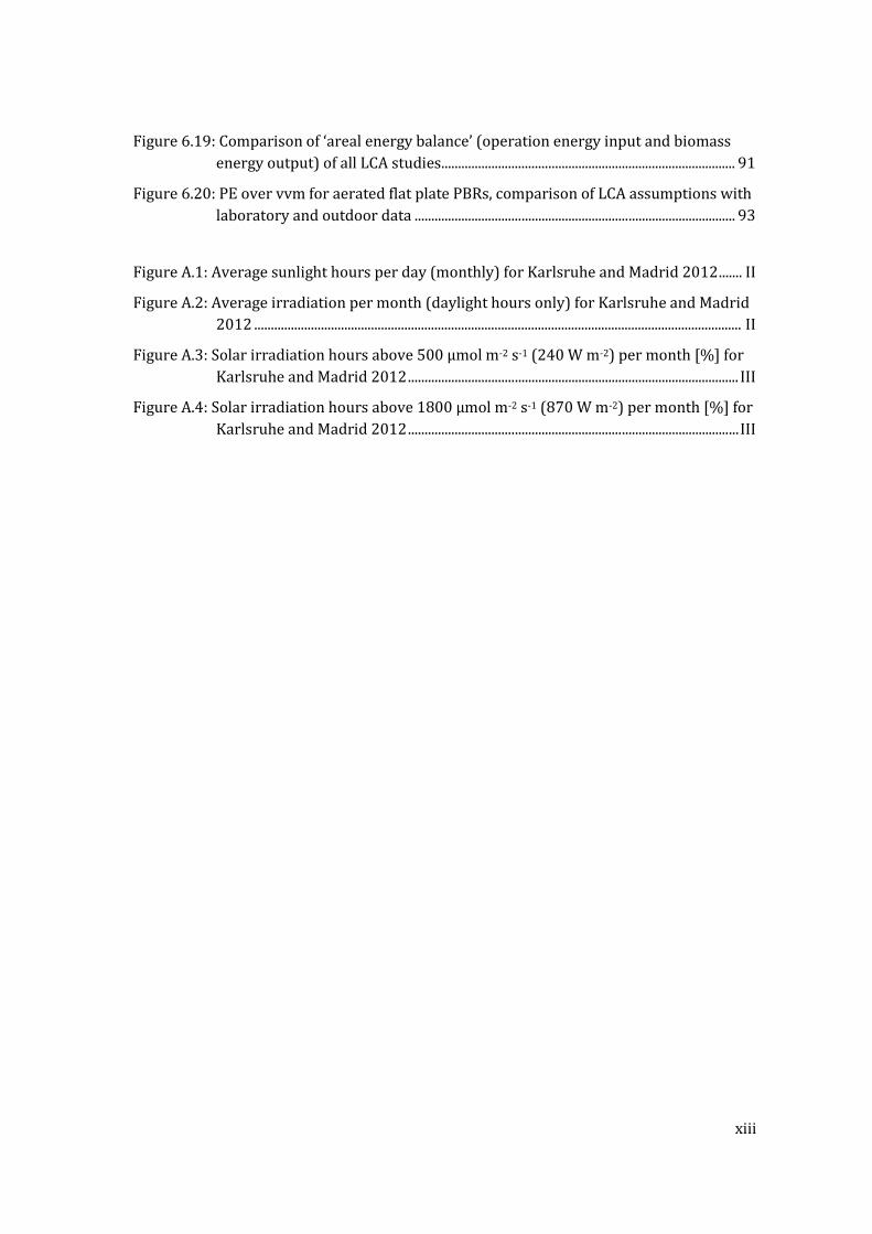
List of tables
Table 2.1: LCA studies reviewed within the European AquaFUELS project (Slade et al. 2011b). .............................................................................................................................................. 9
Table 2.2: Overview over previous LCA studies about microalgae biofuels production ...... 11
Table 2.3: Title and short description of other reviews about microalgae biofuels production .................................................................................................................................... 16
Table 4.1: Maximum volumetric productivities and corresponding biomass concentration for different aeration rates and light intensities as measured in Hu and Richmond (1996) ...................................................................................................................... 43
Table 4.2: Parameters to calculate the PE(vvm) for different light intensities, based on data of (Hu and Richmond 1996) ................................................................................................. 48
Table 4.3: Functions to determine temperature correction factors for triangular and Gaussian distribution ............................................................................................................... 52
Table 4.4: Parameters to calculate temperature correction factors ............................................. 52
Table 4.5: Correction factors for passive temperature control ....................................................... 53
Table 4.6: Laboratory versus outdoor conditions and assumed consequences for the core model .............................................................................................................................................. 55
Table 4.7: Data of outdoor pilot plant studies ........................................................................................ 57
Table 4.8: Parameters to calculate the areal productivity based on the aeration rate ......... 58
Table 5.1: Photobioreactor design parameters ..................................................................................... 61
Table 5.2: Parameters to calculate operation energy.......................................................................... 62
Table 5.3: Pressure drop – sources and literature values ................................................................. 62
Table 5.4: Parameters to calculate the energy demand for reactor material ............................ 63
Table 5.5: Parameters to calculate energy demand for biomass supplies ................................. 65
Table 5.6: Parameters to calculate the energy demand for biogas production and biomethane output ................................................................................................................... 67
Table 5.7: Base case – important parameters ........................................................................................ 67
Table 5.8: Cumulative energy demand scenarios ................................................................................. 68
Table 5.9: Temperature correction factors and night-time operation rate for Karlsruhe and Madrid ............................................................................................................................................ 70
Table 5.10: Location and cultivation period – input parameters, based on (Huld 2013) .... 70
Table 6.1: Operation and productivity parameters (base case) ..................................................... 71
Table 6.2: Resource demand per hectare and year, resulting energy demand and NER (base case) .................................................................................................................................... 72
x
Table 6.3: MJeq per MJ biomethane of each process for different CED scenarios (applied to base case) ...................................................................................................................................... 74
Table 6.4: Clustering of NER contributions for the analysis ............................................................. 76
Table 6.5: Operation and productivity parameters at different aeration rates as indicated in Figure 6.6 ................................................................................................................................. 78
Table 6.6: Operation and productivity parameters at different cultivation times as indicated in Figure 6.14 .......................................................................................................... 84
Table 6.7: Operation and productivity parameters at different cultivation times as indicated in Figure 6.15 .......................................................................................................... 85
Table 6.8: Resource demand per hectare and year, resulting energy input and NER (best case) ................................................................................................................................................ 87
Table 6.9: Comparison with previous studies – system boundaries ............................................ 89
Table 6.10: Comparison with previous studies – important assumptions concerning operation energy and biomass yield ................................................................................. 90
Table 6.11: Summary of comparison of different LCA studies: NER, system boundaries, CER, and PE .................................................................................................................................. 95
Table A.1: Example of irradiation and temperature data for Karlsruhe and Madrid (01.03.2012) .................................................................................................................................... I
Table A.2: Ecoinvent processes (full name) used to model the CED .............................................. IV
Table A.3: CED of energetic relevant flows ............................................................................................... IV
Table A.4: CED of different photobioreactor materials ....................................................................... IV
Table A.5: Links and further information of current and previous large algae biofuels projects ............................................................................................................................................. V
xi
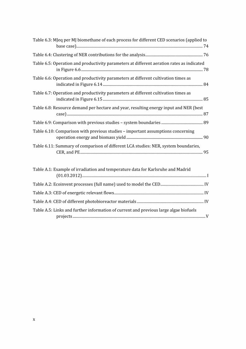
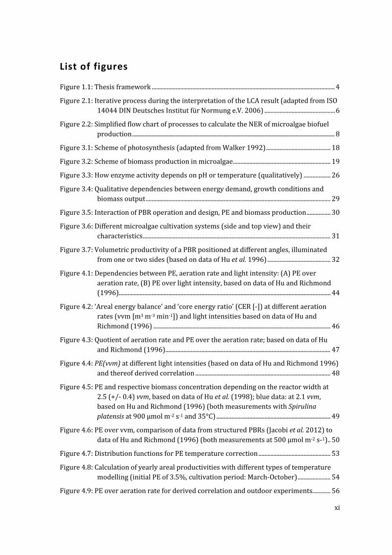
List of figures
Figure 1.1: Thesis framework .......................................................................................................................... 4
Figure 2.1: Iterative process during the interpretation of the LCA result (adapted from ISO 14044 DIN Deutsches Institut für Normung e.V. 2006) ............................................... 6
Figure 2.2: Simplified flow chart of processes to calculate the NER of microalgae biofuel production ....................................................................................................................................... 8
Figure 3.1: Scheme of photosynthesis (adapted from Walker 1992) ........................................... 18
Figure 3.2: Scheme of biomass production in microalgae ................................................................. 19
Figure 3.3: How enzyme activity depends on pH or temperature (qualitatively) .................. 26
Figure 3.4: Qualitative dependencies between energy demand, growth conditions and biomass output ........................................................................................................................... 29
Figure 3.5: Interaction of PBR operation and design, PE and biomass production ................ 30
Figure 3.6: Different microalgae cultivation systems (side and top view) and their characteristics ............................................................................................................................. 31
Figure 3.7: Volumetric productivity of a PBR positioned at different angles, illuminated from one or two sides (based on data of Hu et al. 1996) .......................................... 32
Figure 4.1: Dependencies between PE, aeration rate and light intensity: (A) PE over aeration rate, (B) PE over light intensity, based on data of Hu and Richmond (1996)............................................................................................................................................. 44
Figure 4.2: ‘Areal energy balance’ and ‘core energy ratio’ (CER [-]) at different aeration rates (vvm [m3 m-3 min-1]) and light intensities based on data of Hu and Richmond (1996) ...................................................................................................................... 46
Figure 4.3: Quotient of aeration rate and PE over the aeration rate; based on data of Hu and Richmond (1996) .............................................................................................................. 47
Figure 4.4: PE(vvm) at different light intensities (based on data of Hu and Richmond 1996) and thereof derived correlation .......................................................................................... 48
Figure 4.5: PE and respective biomass concentration depending on the reactor width at 2.5 (+/- 0.4) vvm, based on data of Hu et al. (1998); blue data: at 2.1 vvm, based on Hu and Richmond (1996) (both measurements with Spirulina platensis at 900 µmol m-2 s-1 and 35°C) ............................................................................ 49
Figure 4.6: PE over vvm, comparison of data from structured PBRs (Jacobi et al. 2012) to data of Hu and Richmond (1996) (both measurements at 500 µmol m-2 s-1) .. 50
Figure 4.7: Distribution functions for PE temperature correction ................................................ 53
Figure 4.8: Calculation of yearly areal productivities with different types of temperature modelling (initial PE of 3.5%, cultivation period: March-October) ...................... 54
Figure 4.9: PE over aeration rate for derived correlation and outdoor experiments. ........... 56
xii
Figure 4.10: Areal energy balance for outdoor pilot plants, short term and long term measurements ............................................................................................................................ 56
Figure 5.1: Flow chart of all processes modelled to calculate the NER, inclusion of core model .............................................................................................................................................. 60
Figure 5.2: Scheme of generic flat plate PBR .......................................................................................... 61
Figure 5.3: PE(vvm) as determined for aeration rates below 1 vvm at 500 µmol m-2 s-1 (detail of Figure 4.4) ................................................................................................................. 69
Figure 6.1: Energy input (cumulative energy demand) and output (HHV biomethane) per hectare and year (base case) ................................................................................................ 72
Figure 6.2: Areal operation energy, energy content in biomass (intermediate) and biomethane energy (base case) ........................................................................................... 73
Figure 6.3: NER for different CED scenarios (applied to base case) ............................................. 74
Figure 6.4: Interaction of other parameters with different CED scenarios ................................ 75
Figure 6.5: NER depending on the aeration rate (base case + ‘CED 0.7’) .................................... 76
Figure 6.6: NER depending on the aeration rate, detailed analysis of contributions (base case + ’CED 0.7) .......................................................................................................................... 77
Figure 6.7: Energy input and output at different aeration rates as indicated in Figure 6.6 78
Figure 6.8: NER depending on the aeration rate, influence of CED scenarios .......................... 79
Figure 6.9: NER depending on the aeration rate, influence of reduced pressure drop ......... 79
Figure 6.10: NER depending on the aeration rate, influence of pipeline .................................... 80
Figure 6.11: Energy input and output of an ‘empty’ compared to a ‘structured’ PBR (Karlsruhe, Mar-Oct, ‘CED 0.7’, ’50 mbar’) ...................................................................... 81
Figure 6.12: NER depending on the aeration rate – comparison Karlsruhe and Madrid (Mar-Oct, ‘CED 0.7’, ’50 mbar’)............................................................................................. 82
Figure 6.13: Energy inputs and outputs for cultivation in Karlsruhe and Madrid at 0.6 vvm (Mar-Oct, ‘CED 0.7’, ’50 mbar’)............................................................................................. 83
Figure 6.14: NER depending on the cultivation period (Karlsruhe, 0.25 vvm ‘CED 0.7, 50 mbar’)....................................................................................................................................... 84
Figure 6.15: NER depending on the cultivation period (Madrid, 0.25 vvm ‘CED 0.7, 50 mbar’)....................................................................................................................................... 84
Figure 6.16: NER at different cultivation periods and aeration rates (Karlsruhe, ‘CED 0.7, 50 mbar’)....................................................................................................................................... 85
Figure 6.17: Energy input and output best case (Madrid, Mar-Oct, 0.25 vvm, CED 0.7, 50 mbar) ........................................................................................................................................ 86
Figure 6.18: Comparison of NER of other studies to this study with the respective adapted system boundaries .................................................................................................................... 88
xiii
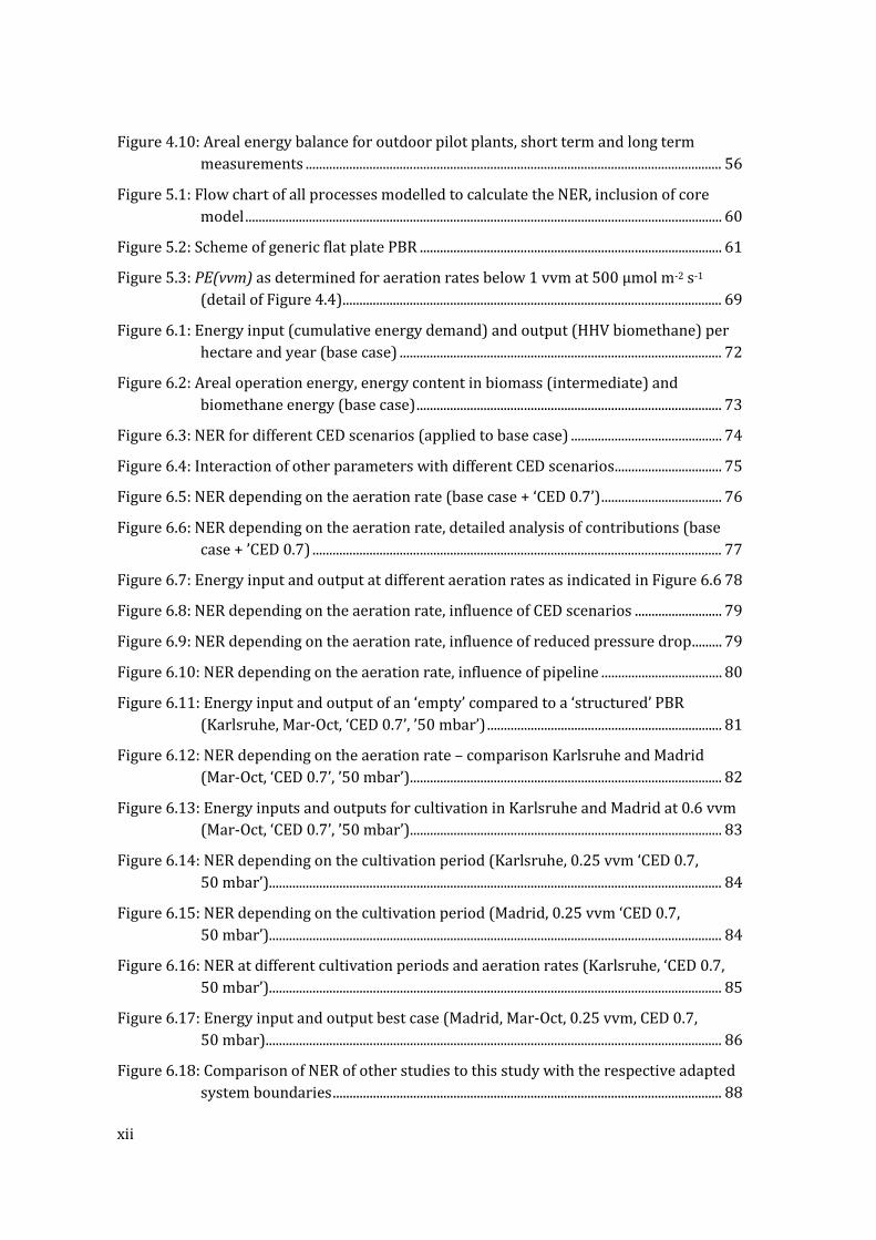
Figure 6.19: Comparison of ‘areal energy balance’ (operation energy input and biomass energy output) of all LCA studies ........................................................................................ 91
Figure 6.20: PE over vvm for aerated flat plate PBRs, comparison of LCA assumptions with laboratory and outdoor data ................................................................................................ 93
Figure A.1: Average sunlight hours per day (monthly) for Karlsruhe and Madrid 2012 ....... II
Figure A.2: Average irradiation per month (daylight hours only) for Karlsruhe and Madrid 2012 .................................................................................................................................................. II
Figure A.3: Solar irradiation hours above 500 µmol m-2 s-1 (240 W m-2) per month [%] for Karlsruhe and Madrid 2012 ................................................................................................... III
Figure A.4: Solar irradiation hours above 1800 µmol m-2 s-1 (870 W m-2) per month [%] for Karlsruhe and Madrid 2012 ................................................................................................... III
xiv
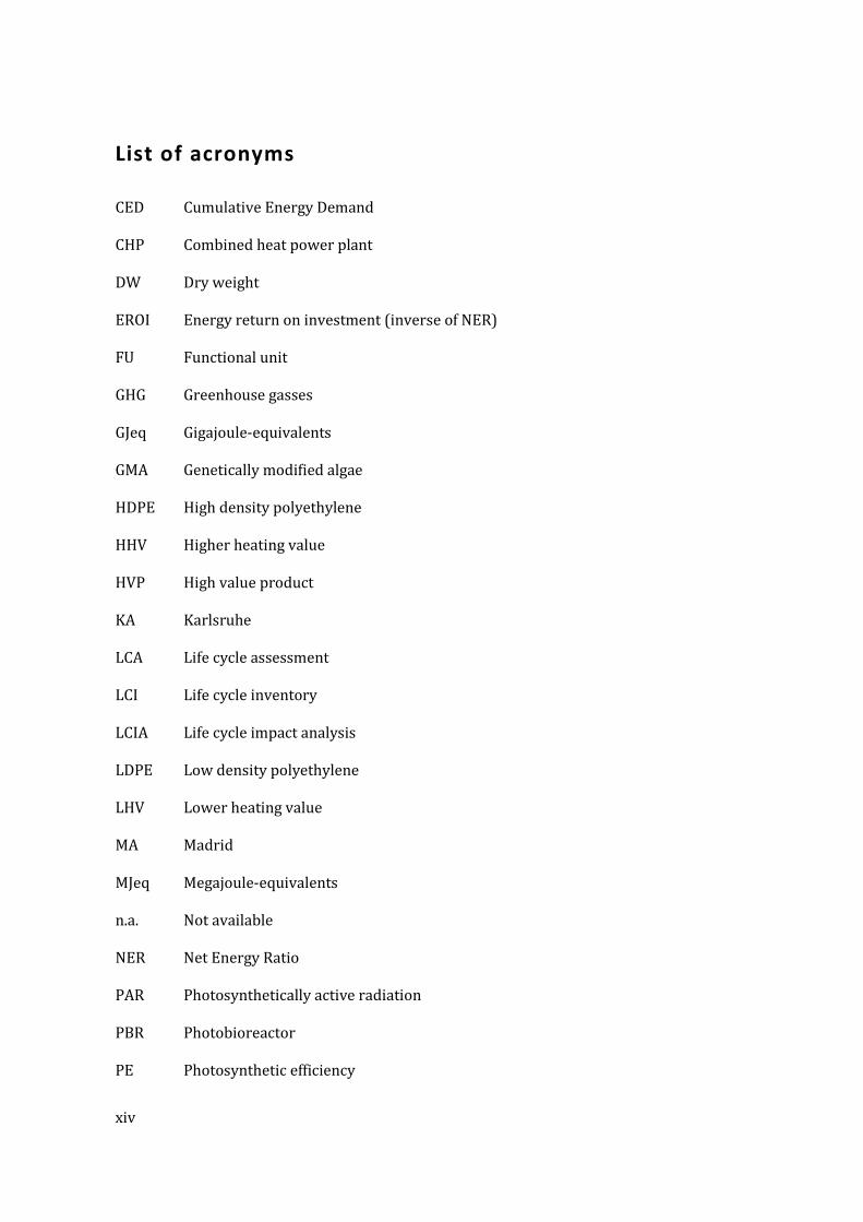
List of acronyms
CED Cumulative Energy Demand
CHP Combined heat power plant
DW Dry weight
EROI Energy return on investment (inverse of NER)
FU Functional unit
GHG Greenhouse gasses
GJeq Gigajoule-equivalents
GMA Genetically modified algae
HDPE High density polyethylene
HHV Higher heating value
HVP High value product
KA Karlsruhe
LCA Life cycle assessment
LCI Life cycle inventory
LCIA Life cycle impact analysis
LDPE Low density polyethylene
LHV Lower heating value
MA Madrid
MJeq Megajoule-equivalents
n.a. Not available
NER Net Energy Ratio
PAR Photosynthetically active radiation
PBR Photobioreactor
PE Photosynthetic efficiency

xv
PETG Polyethylene terephthalate granulate
PFD Photon flux density
VS Volatile solids
xvi
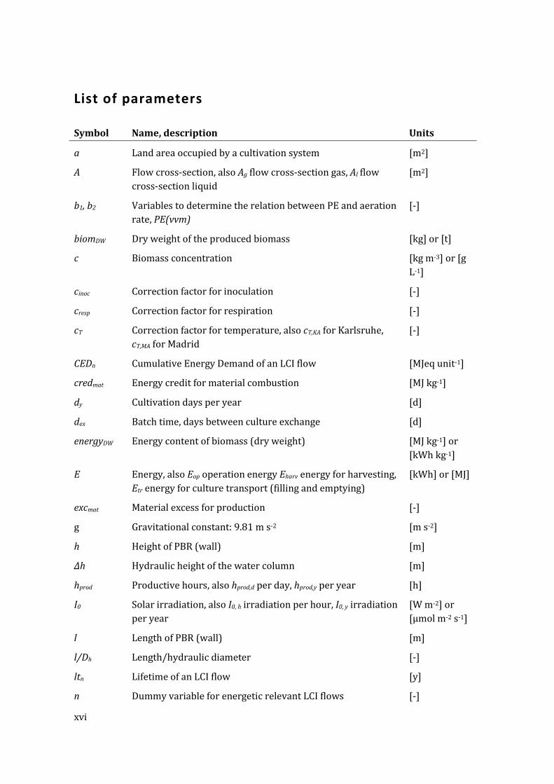
List of parameters
Symbol Name, description Units
a Land area occupied by a cultivation system [m2]
A Flow cross-section, also Ag flow cross-section gas, Al flow cross-section liquid
[m2]
b1, b2 Variables to determine the relation between PE and aeration rate, PE(vvm)
[-]
biomDW Dry weight of the produced biomass [kg] or [t]
c Biomass concentration [kg m-3] or [g L-1]
cinoc Correction factor for inoculation [-]
cresp Correction factor for respiration [-]
cT Correction factor for temperature, also cT,KA for Karlsruhe, cT,MA for Madrid
[-]
CEDn Cumulative Energy Demand of an LCI flow [MJeq unit-1]
credmat Energy credit for material combustion [MJ kg-1]
dy Cultivation days per year [d]
dex Batch time, days between culture exchange [d]
energyDW Energy content of biomass (dry weight) [MJ kg-1] or [kWh kg-1]
E Energy, also Eop operation energy Eharv energy for harvesting, Etr energy for culture transport (filling and emptying)
[kWh] or [MJ]
excmat Material excess for production [-]
g Gravitational constant: 9.81 m s-2 [m s-2]
h Height of PBR (wall) [m]
Δh Hydraulic height of the water column [m]
hprod Productive hours, also hprod,d per day, hprod,y per year [h]
I0 Solar irradiation, also I0, h irradiation per hour, I0, y irradiation per year
[W m-2] or [µmol m-2 s-1]
l Length of PBR (wall) [m]
l/Dh Length/hydraulic diameter [-]
ltn Lifetime of an LCI flow [y]
n Dummy variable for energetic relevant LCI flows [-]
xvii
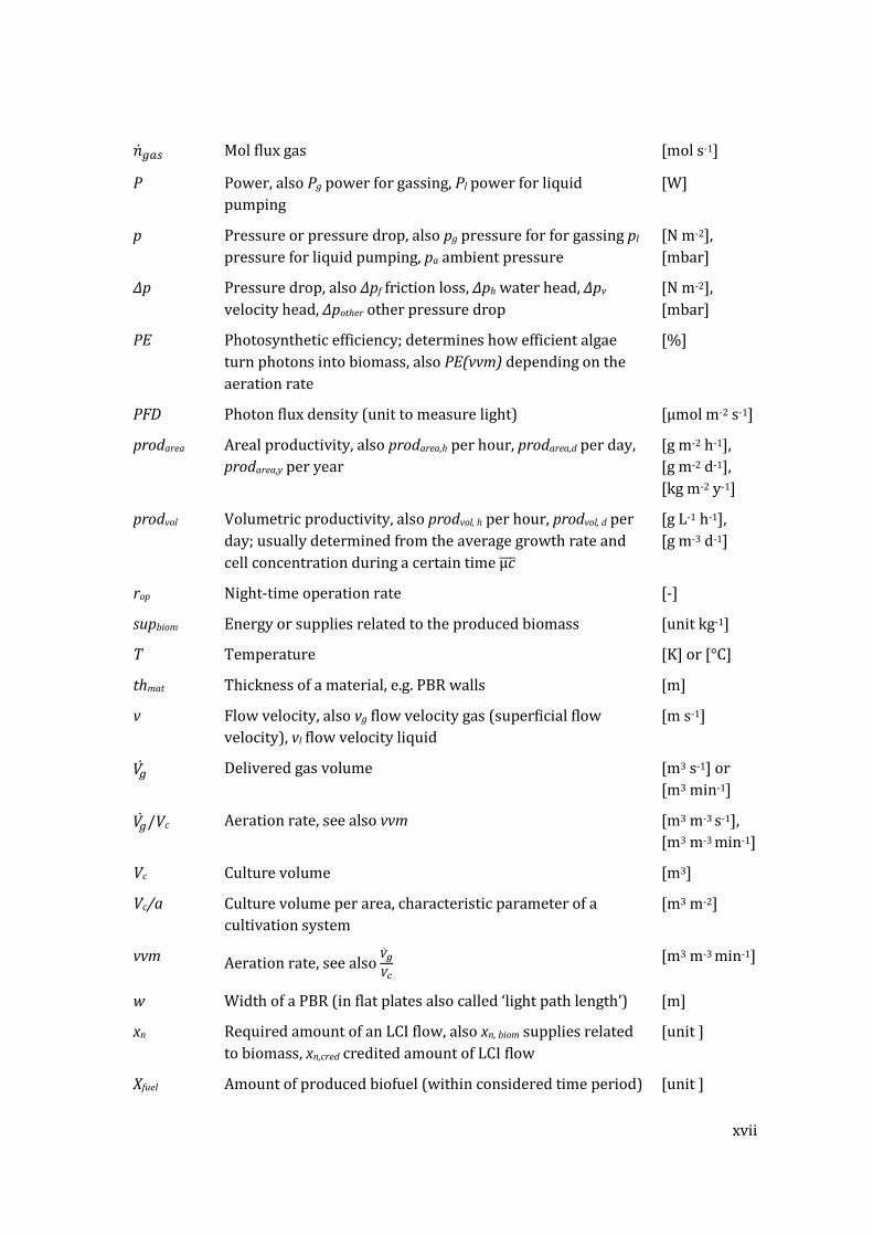
�̇�𝑔𝑔𝑔 Mol flux gas [mol s-1]
P Power, also Pg power for gassing, Pl power for liquid pumping
[W]
p Pressure or pressure drop, also pg pressure for for gassing pl
pressure for liquid pumping, pa ambient pressure [N m-2], [mbar]
Δp Pressure drop, also Δpf friction loss, Δph water head, Δpv velocity head, Δpother other pressure drop
[N m-2], [mbar]
PE Photosynthetic efficiency; determines how efficient algae turn photons into biomass, also PE(vvm) depending on the aeration rate
[%]
PFD Photon flux density (unit to measure light) [µmol m-2 s-1]
prodarea Areal productivity, also prodarea,h per hour, prodarea,d per day, prodarea,y per year
[g m-2 h-1], [g m-2 d-1], [kg m-2 y-1]
prodvol Volumetric productivity, also prodvol, h per hour, prodvol, d per day; usually determined from the average growth rate and cell concentration during a certain time µ𝑐���
[g L-1 h-1], [g m-3 d-1]
rop Night-time operation rate [-]
supbiom Energy or supplies related to the produced biomass [unit kg-1]
T Temperature [K] or [°C]
thmat Thickness of a material, e.g. PBR walls [m]
v Flow velocity, also vg flow velocity gas (superficial flow velocity), vl flow velocity liquid
[m s-1]
𝑉�̇� Delivered gas volume [m3 s-1] or [m3 min-1]
𝑉�̇�/Vc Aeration rate, see also vvm [m3 m-3 s-1], [m3 m-3 min-1]
Vc Culture volume [m3]
Vc/a Culture volume per area, characteristic parameter of a cultivation system
[m3 m-2]
vvm Aeration rate, see also �̇�𝑔
𝑉𝑐 [m3 m-3 min-1]
w Width of a PBR (in flat plates also called ‘light path length’) [m]
xn Required amount of an LCI flow, also xn, biom supplies related to biomass, xn,cred credited amount of LCI flow
[unit ]
Xfuel Amount of produced biofuel (within considered time period) [unit ]
xviii
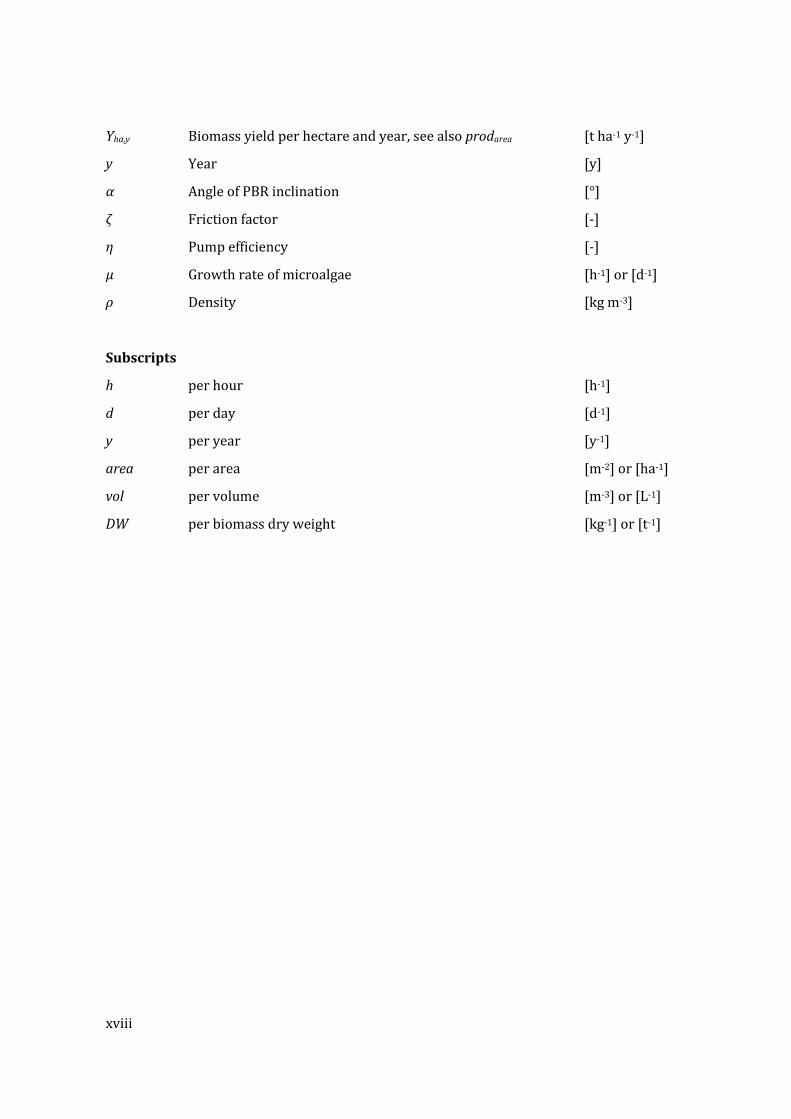
Yha,y Biomass yield per hectare and year, see also prodarea [t ha-1 y-1]
y Year [y]
𝛼 Angle of PBR inclination [°]
ζ Friction factor [-]
η Pump efficiency [-]
𝜇 Growth rate of microalgae [h-1] or [d-1]
ρ Density [kg m-3]
Subscripts
h per hour [h-1]
d per day [d-1]
y per year [y-1]
area per area [m-2] or [ha-1]
vol per volume [m-3] or [L-1]
DW per biomass dry weight [kg-1] or [t-1]
1
1 Introduction
1.1 Why microalgae biofuels?
Microalgae are small organisms that live in the water and use solar energy to grow. They have been cultivated for a long time to produce food, feed and other substances. Microalgae biomass can also be used to produce biofuels, such as (bio-) ethanol, diesel, hydrogen or methane. Since the Second World War there have been repeated attempts to produce biofuels from microalgae (Borowitzka 2013). Initial motivation was the independence of external fuel supply and/or saving fossil resources. The idea has recently received a boost due to a specific feature of microalgae: unlike other biofuel feedstock, microalgae do not compete with food production for arable land. Like plants, microalgae grow quickly with concentrated CO2 and can thus re-use CO2 from other resources.
To produce biofuels from microalgae, microalgae must be cultivated on large scale in technical systems (with nutrients and CO2). The biomass must be harvested and converted into a fuel. The energy needed to provide electricity and materials for all processes along the biofuel production chain can be assessed with the so-called ‘cumulative energy demand’ (CED), a method of life cycle assessment (LCA). The total energy demand of all processes and materials related to the biofuel energy content is called net energy ratio (NER).
Prerequisite to produce microalgae biofuels is a NER less than one: Less energy should be required to produce the fuel than energy is provided with the fuel. However, microalgae cultivation requires much energy so that a NER<1 is not possible today (Morweiser et al. 2011). Despite intensive research, no commercial microalgae biofuel production plant exists and many previous attempts to produce microalgae biofuels on large scale have failed (Tredici 2003, Borowitzka 2013).
1.2 Problem definition
LCA studies about microalgae biofuels production calculated NER results above and below one (Sills et al. 2011). Almost all studies about microalgae biofuels production emphasise the need for technology development “to make algae biofuels a sustainable, commercial reality” (Sander and Murthy 2010).
The NER is the result of a model and, as such, depends on assumptions about system boundaries, input parameters and underlying functions. Different NER results and therefore different expectations regarding the potential development of the technology can be due to all three aspects:
The first and most obvious reason for different NER results are incomplete system boundaries. For example, some studies assessed only the operation energy to cultivate
1 Introduction
2
microalgae, others included energy demand for harvesting and processing the biomass but omit energy for supplies and materials. Not surprisingly, Slade et al. (2011a) found that “the most optimistic results [of the NER] come from the systems which are least complete”. Second, the variety of cultivation methods, harvesting methods and processes to produce biofuels results in different NERs.
The third and maybe most important reason for different NER results are the underlying functions or more precisely, whether a correlation between core model parameters has been considered or not.
Regarding the last aspect, previous studies found that the NER depends strongly on the operation energy demand (Stephenson et al. 2010, Weinberg et al. 2012). They also found that the expected biomass yield strongly influences the NER result (Zamolla et al. 2011, Slade et al. 2011b). Further information connects these findings: it is “well-established and clearly evident” (Hu and Richmond 1996) that the operation energy determines the cultivation conditions and therefore the biomass yield. This dependency has not yet been considered to calculate and predict the NER of microalgae biofuels production.
In summary, no previous LCA study calculated the NER of microalgae biofuels production considering that the biomass yield depends on the operation energy – even though (a) both parameters considerably determine the NER and (b) a correlation between these parameters is evident.
1.3 Objectives and scope
The aim of this study is to investigate dependencies between key parameters of microalgae cultivation and model the net energy ratio (NER) of microalgae biofuel production based on these dependencies.
This aim can be expressed in the following research questions:
1.) Why and how do important model parameters depend on each other? 2.) What are the consequences for the NER with regard to the dependencies? 3.) What are the consequences regarding technology development?
The approach shall help to better understand important interactions regarding microalgae cultivation. It shall also allow calculating more reliable NERs of microalgae biofuels production. The results of this dissertation shall help decision makers in policy, society and industry to better evaluate the potential of microalgae biofuels production.
This thesis focusses on the energy balance of biofuels production from microalgae mass cultivation in closed photobioreactors. These terms are defined in the following in order to set the scope of this dissertation:
Microalgae mass cultivation involves – in contrary to harvesting microalgae from their natural environment – the provision of a cultivation system, nutrients and CO2 supply on a large scale. Furthermore, it implies changing light, temperature and weather conditions.
The focus of this study lies on microalgae cultivation in closed photobioreactors (PBRs) since it is expected that improved PBR technology can contribute to a better net energy
1.4 Thesis outline
3
ratio (NER). A lower NER is also expected from genetically modified or specially selected algae – those should not be cultivated in open systems to avoid contamination. Therefore, open cultivation systems which are in contact with the surrounding environment are not examined in this thesis.
Last but not least, this study investigates biofuel production as the main purpose and function of microalgae cultivation. Biofuels as a by-product of another main product is not considered. Apart from methodological issues (about how to assess the NER of a system with several outputs), this has practical reasons: very few microalgae products leave residual biomass. For example, the whole algae cell is used to produce food and feed. Furthermore, markets for extracted substances (e.g. antioxidants or pigments) are small.
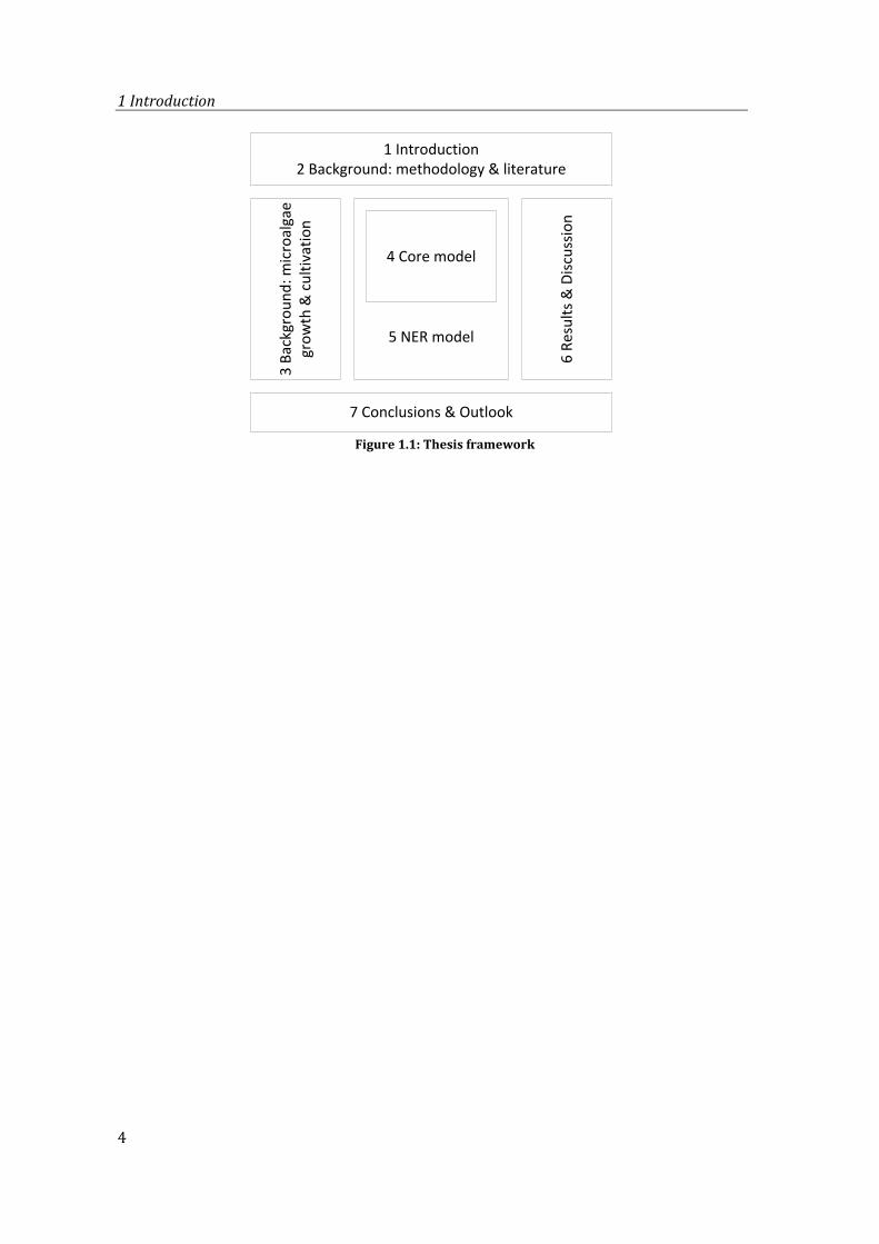
1.4 Thesis outline
In this dissertation it is analysed why and how most important model parameters to determine biomass yield and operation energy are related. For this purpose, a ‘core model’ is developed describing the dependencies. This model is used to calculate the net energy ratio (NER) of microalgae biofuels production.
The thesis is structured as follows (Figure 1.1): Chapter 2 provides the methodological background to assess the net energy ratio of microalgae biofuels production and the literature review highlighting the research gaps.
Chapter 3 explains the fundamental principles, requirements and limitations of microalgae growth and cultivation. Those are essential to understand why and how core model parameters are related. The most important equations to calculate biomass yield and operation energy are introduced.
In chapter 4, the ‘core model’ is developed which describes a correlation between important parameters to calculate operation energy and biomass yield. The model is validated with further laboratory and outdoor data.
Chapter 5 defines all other upstream and downstream assumptions and parameters to calculate the NER of microalgae biofuels production. Scenarios and parameter variations are introduced.
Chapter 6 shows the NER results under different assumptions. A best case NER is defined and compared to the NER results of previous LCA studies. The reasons for different results are analysed. Limitations of this thesis are discussed and the transferability of method to other systems is described.
Finally, chapter 7 summarises the answers to the research questions and gives suggestions for further research.
1 Introduction
4
4 Core model
3 Ba
ckgr
ound
: mic
roal
gae
grow
th &
cul
tivat
ion
7 Conclusions & Outlook
1 Introduction 2 Background: methodology & literature
6 Re
sults
& D
iscus
sion
5 NER model
Figure 1.1: Thesis framework
5
2 Methodological background and literature review
This chapter describes the methodological and literature background of the study.
Section 2.1 presents the methodology to calculate the NER of microalgae biofuels production based on the LCA approach. Section 2.2 gives a review about the most important literature about the NER of microalgae biofuels production with a focus on the research gaps.
2.1 Methodology
This section explains the method of Life Cycle Assessment (LCA), the Cumulative Energy Demand (CED) as a method within LCA and the net energy ratio (NER) as characteristic quotient which can be calculated with the above definitions.
2.1.1 Life cycle assessment (LCA)
The net energy ratio of microalgae biofuels production should include all direct and indirect energy inputs and outputs along the production chain. These apply for: providing the resources for cultivation, harvesting and processing the biomass and, if applicable, disposal or recycling processes. Those can be assessed with the method of Life Cycle Assessment (LCA). LCA principles and framework, requirements and guidelines are described in the ISO guidelines 14040 and 14044 respectively (DIN Deutsches Institut für Normung e.V. 2006, 2006). The four interdependent stages of an LCA are:
1.) Goal and scope definition 2.) Live cycle inventory (LCI) 3.) Live cycle impact assessment (LCIA) 4.) Interpretation of results
Goal and scope define the purpose and recipient of the LCA: What question should be answered and who wants to know the answer? For example, an LCA for industry can identify weak points along the microalgae production chain or trade-offs between different processes. The goal and scope determines also the main function of the investigated process: the functional unit (FU). All inputs and outputs are usually related to the FU.
The life cycle inventory (LCI) describes the mass and energy flows of the processes (e.g. cultivating microalgae and producing biofuels) and how they are related; it is the core of the LCA. The assumptions taken in the LCI: boundary conditions, parameters and their dependencies determine the LCA result. Therefore, the LCI should – as any model – reflect the reality as good as possible.
LCIA methods linearly assign one or several ‘environmental impacts’ of different ‘categories’ to each mass or energy flow of the LCI. For example, a process can require resources (energy, land, water, …), cause emissions (CO2, SO2, …), or have other effects on
2 Methodological background and literature review
6
the environment. Data for relations between flows and impacts (‘characterisation factors’) result from physical, toxicological and other measurements. For a variety of processes (e.g. the production of 1 kg of steel) the ‘environmental impacts’ have already been calculated in previous LCAs. Results are stored in large databases like the German GaBi or the Suisse ecoinvent and can be used for further calculations. The data can be evaluated, combined and modified with LCA software, such as umberto, openLCA or SimaPro.
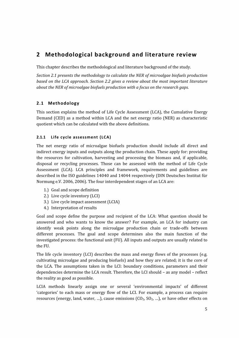
The result of the LCA depends on the data and decisions of the previous steps. Are they adequate to fulfill the purpose of the study? If not they must be verified or changed. The process of LCA is thus iterative (Figure 2.1).
Goal and scope definition
Impact assessmentApplications: Product development
and improvement Strategic planning Public policy making Marketing
Identifcation of significant issues
Conclusions Limitations
Recommendations
Inventory analysis
Evaluation and check Are data and results: Complete Consistent Sensitive to changes Relevant for the
application
Interpretation
LCA framework
Figure 2.1: Iterative process during the interpretation of the LCA result (adapted from ISO 14044
DIN Deutsches Institut für Normung e.V. 2006)
2.1.2 Cumulative Energy Demand (CED)
The ‘Cumulative Energy Demand’ (CED) is an LCIA method and as such a potential part of an LCA. The CED reflects how much energy is ‘withdrawn from nature’ in order to provide a certain product or process. For example, the CED to provide 1 kWh electricity from coal reflects the energy content of the extracted coal, but also the energy for resources needed to burn the coal and transport the resulting heat or electricity. Background and methodology to determine the CED are described in detail in (Hischier and Weidema 2009) and (Verein deutscher Ingenieure (VDI) 2012).
All resources needed to produce microalgae biofuels, such as electricity, fertilisers or materials have a CED. The CED in this study is calculated with the software umberto (NXT LCA 7.1) and the method as documented in Hischier and Weidema (2009). This method accounts fossil resources with their higher heating value (HHV) and renewable resources with 1 MJ-equivalent (MJeq) per MJ produced electricity, following the approach of (Frischknecht et al. 1998). The Verein Deutscher Ingenieure (VDI) suggests using the lower heating value (LHV) to calculate the CED, though states that it is “more appropriate” using the HHV value regarding the CED as an indicator for resource efficiency (2012).
2.1 Methodology
7
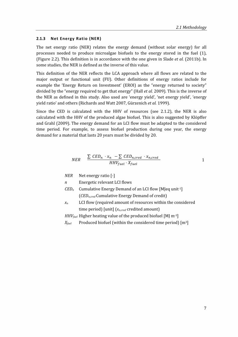
2.1.3 Net Energy Ratio (NER)
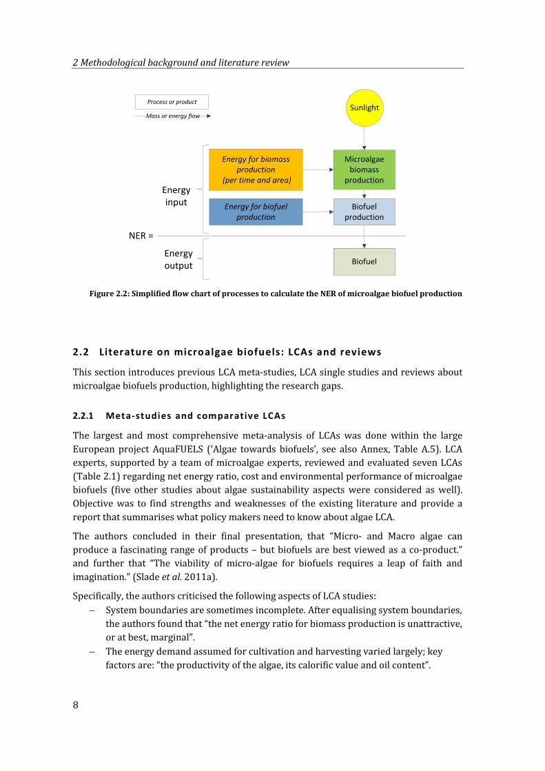
The net energy ratio (NER) relates the energy demand (without solar energy) for all processes needed to produce microalgae biofuels to the energy stored in the fuel (1), (Figure 2.2). This definition is in accordance with the one given in Slade et al. (2011b). In some studies, the NER is defined as the inverse of this value.
This definition of the NER reflects the LCA approach where all flows are related to the major output or functional unit (FU). Other definitions of energy ratios include for example the ‘Energy Return on Investment’ (EROI) as the “energy returned to society” divided by the “energy required to get that energy” (Hall et al. 2009). This is the inverse of the NER as defined in this study. Also used are ‘energy yield’, ‘net energy yield’, ‘energy yield ratio’ and others (Richards and Watt 2007, Gürzenich et al. 1999).
Since the CED is calculated with the HHV of resources (see 2.1.2), the NER is also calculated with the HHV of the produced algae biofuel. This is also suggested by Klöpffer and Grahl (2009). The energy demand for an LCI flow must be adapted to the considered time period. For example, to assess biofuel production during one year, the energy demand for a material that lasts 20 years must be divided by 20.
𝑁𝑁𝑁 = ∑(𝐶𝑁𝐶𝑛 ⋅ 𝑥𝑛) − ∑(𝐶𝑁𝐶𝑛,𝑐𝑐𝑐𝑐 ⋅ 𝑥𝑛,𝑐𝑐𝑐𝑐)
𝐻𝐻𝑉𝑓𝑓𝑐𝑓 ⋅ 𝑋𝑓𝑓𝑐𝑓 (1)
NER Net energy ratio [-] n Energetic relevant LCI flows CEDn Cumulative Energy Demand of an LCI flow [MJeq unit-1] (CEDn,cred Cumulative Energy Demand of credit) xn LCI flow (required amount of resources within the considered time period) [unit] (xn,cred credited amount) HHVfuel Higher heating value of the produced biofuel [MJ m-3] Xfuel Produced biofuel (within the considered time period) [m3]
2 Methodological background and literature review
8
Energy for biomass production
(per time and area)
Energy for biofuel production
Process or product
Mass or energy flow
NER =
Energy input
Energy output
Sunlight
Biofuel
Microalgae biomass
production
Biofuel production
Figure 2.2: Simplified flow chart of processes to calculate the NER of microalgae biofuel production
2.2 Literature on microalgae biofuels: LCAs and reviews
This section introduces previous LCA meta-studies, LCA single studies and reviews about microalgae biofuels production, highlighting the research gaps.
2.2.1 Meta-studies and comparative LCAs
The largest and most comprehensive meta-analysis of LCAs was done within the large European project AquaFUELS (‘Algae towards biofuels’, see also Annex, Table A.5). LCA experts, supported by a team of microalgae experts, reviewed and evaluated seven LCAs (Table 2.1) regarding net energy ratio, cost and environmental performance of microalgae biofuels (five other studies about algae sustainability aspects were considered as well). Objective was to find strengths and weaknesses of the existing literature and provide a report that summarises what policy makers need to know about algae LCA.
The authors concluded in their final presentation, that “Micro- and Macro algae can produce a fascinating range of products – but biofuels are best viewed as a co-product.” and further that “The viability of micro-algae for biofuels requires a leap of faith and imagination.” (Slade et al. 2011a).
Specifically, the authors criticised the following aspects of LCA studies: − System boundaries are sometimes incomplete. After equalising system boundaries,
the authors found that “the net energy ratio for biomass production is unattractive, or at best, marginal”.
− The energy demand assumed for cultivation and harvesting varied largely; key factors are: “the productivity of the algae, its calorific value and oil content”.
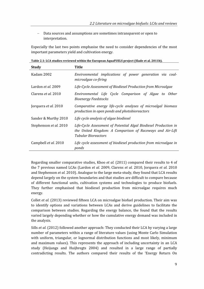
2.2 Literature on microalgae biofuels: LCAs and reviews
9
− Data sources and assumptions are sometimes intransparent or open to interpretation.
Especially the last two points emphasise the need to consider dependencies of the most important parameters yield and cultivation energy.
Table 2.1: LCA studies reviewed within the European AquaFUELS project (Slade et al. 2011b).
Study Title
Kadam 2002 Environmental implications of power generation via coal-microalgae co-firing
Lardon et al. 2009 Life-Cycle Assessment of Biodiesel Production from Microalgae
Clarens et al. 2010 Environmental Life Cycle Comparison of Algae to Other Bioenergy Feedstocks
Jorquera et al. 2010 Comparative energy life-cycle analyses of microalgal biomass production in open ponds and photobioreactors
Sander & Murthy 2010 Life cycle analysis of algae biodiesel
Stephenson et al. 2010 Life-Cycle Assessment of Potential Algal Biodiesel Production in the United Kingdom: A Comparison of Raceways and Air-Lift Tubular Bioreactors
Campbell et al. 2010 Life cycle assessment of biodiesel production from microalgae in ponds
Regarding smaller comparative studies, Khoo et al. (2011) compared their results to 4 of the 7 previous named LCAs (Lardon et al. 2009, Clarens et al. 2010, Jorquera et al. 2010 and Stephenson et al. 2010). Analogue to the large meta-study, they found that LCA results depend largely on the system boundaries and that studies are difficult to compare because of different functional units, cultivation systems and technologies to produce biofuels. They further emphasised that biodiesel production from microalgae requires much energy.
Collet et al. (2013) reviewed fifteen LCA on microalgae biofuel production. Their aim was to identify options and variations between LCAs and derive guidelines to facilitate the comparison between studies. Regarding the energy balance, the found that the results varied largely depending whether or how the cumulative energy demand was included in the analysis.
Sills et al. (2012) followed another approach: They conducted their LCA by varying a large number of parameters within a range of literature values (using Monte Carlo Simulation with uniform, triangular, or lognormal distribution functions and most likely, minimum and maximum values). This represents the approach of including uncertainty in an LCA study (Heijungs and Huijbregts 2004) and resulted in a large range of partially contradicting results. The authors compared their results of the ‘Energy Return On
2 Methodological background and literature review
10
Investment’ (the inverse of the NER) to results of previous studies and concluded that no result is incorrect but “each represents a specific case”. One of the main limitations according to the authors is, that they did not consider whether or how important process parameters are correlated.
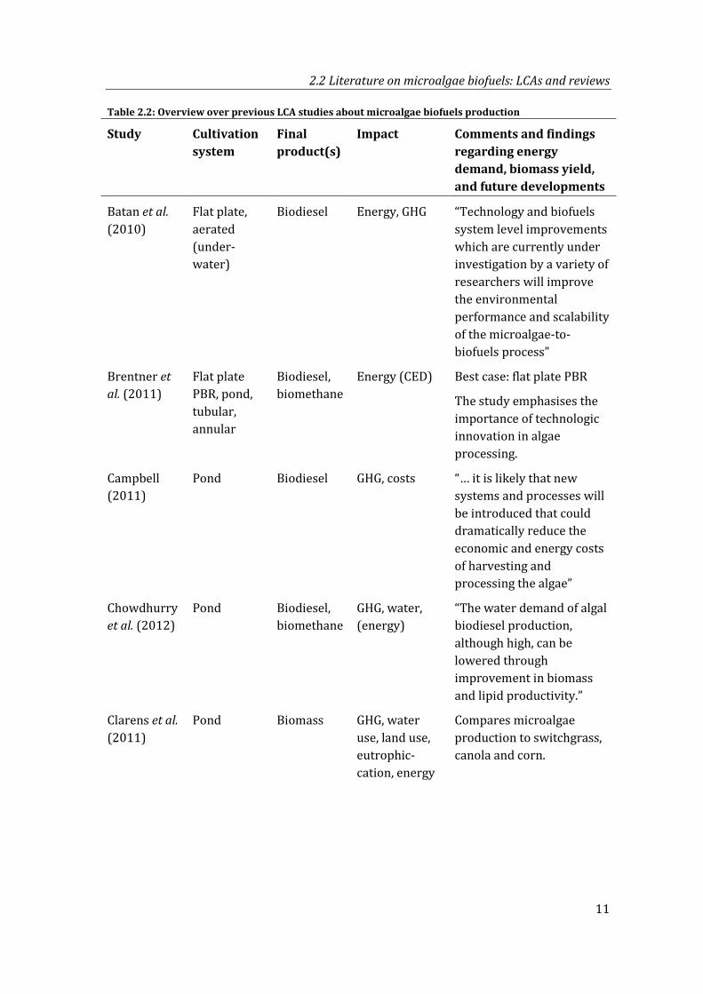
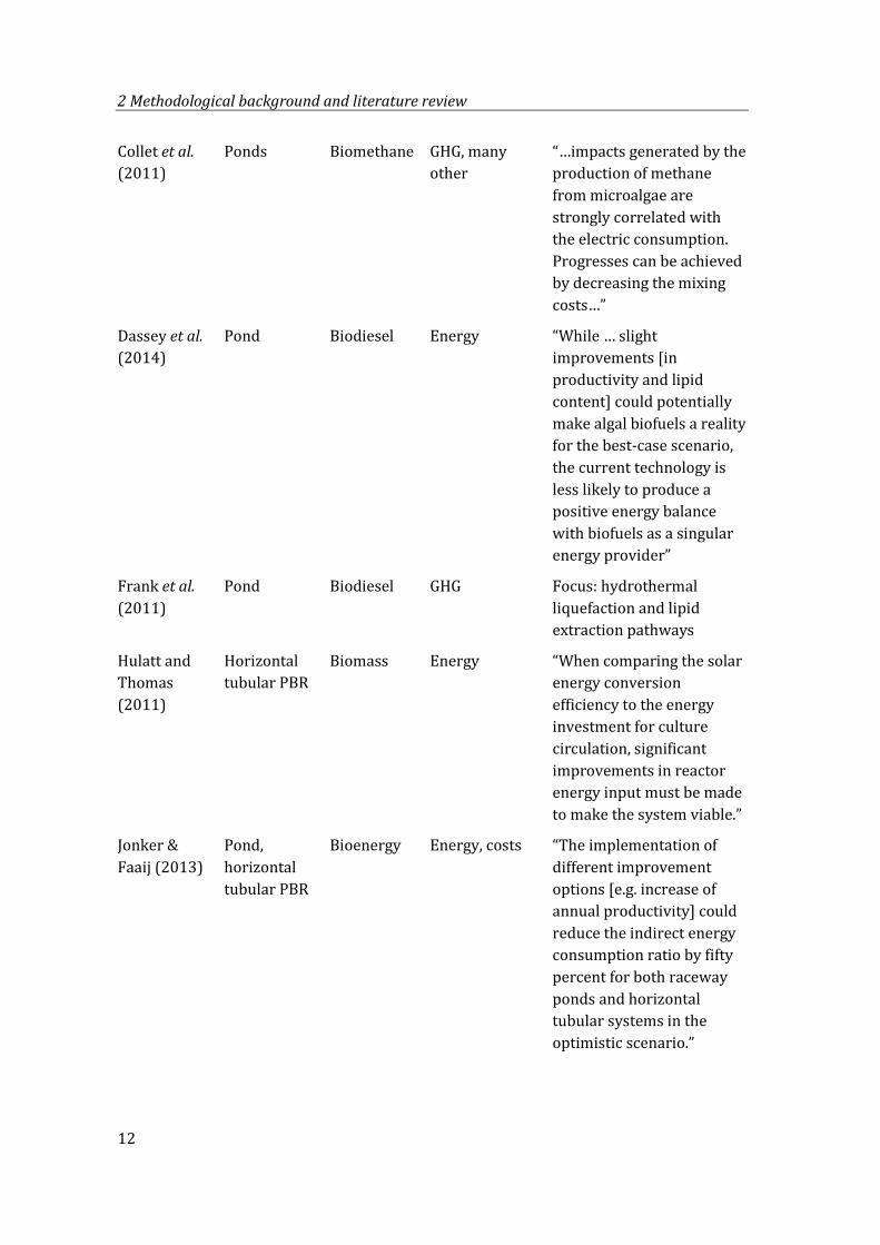
2.2.2 Single LCA studies
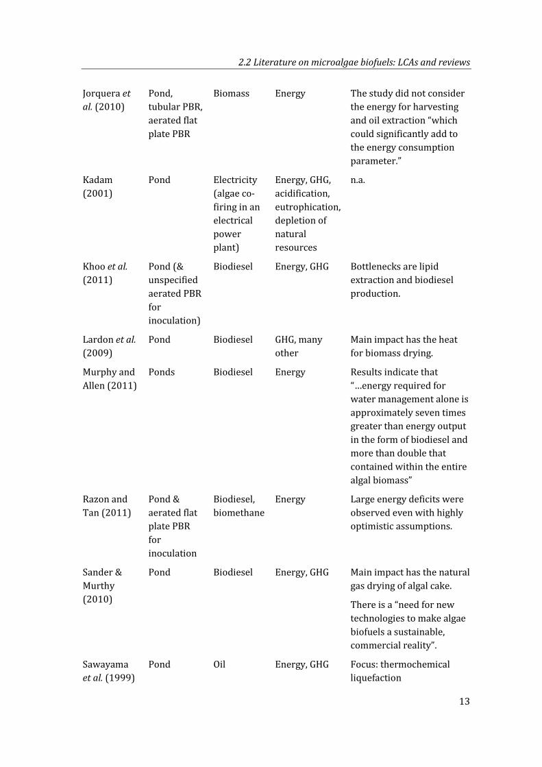
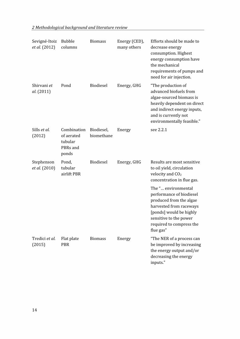
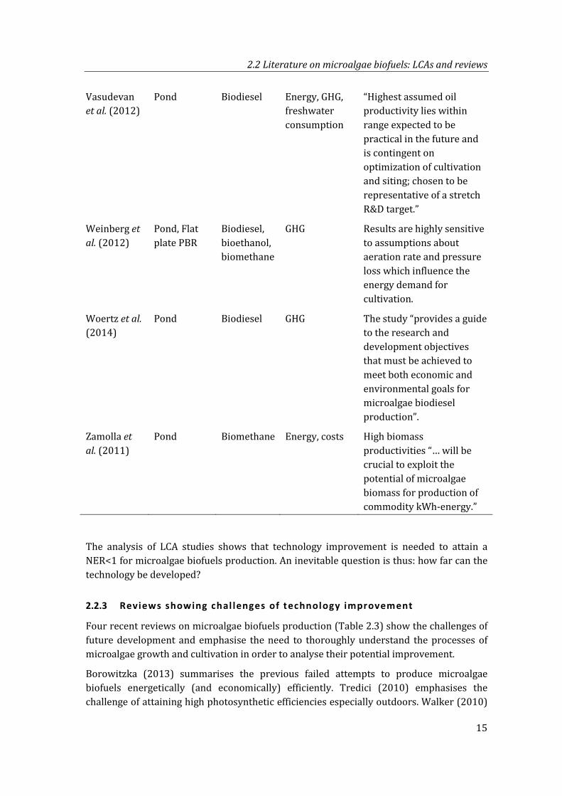
Table 2.2 gives an overview over previous LCA studies, including information about the investigated cultivation system, final product and calculated impact category. Important comments and findings regarding energy demand, biomass yield, and future developments are summarised.
The conclusions and observations of the respective studies emphasise the need to investigate in more detail the dependency between cultivation energy and biomass productivities and their potential development:
− Results are often highly sensitive to parameters that affect productivities and/or cultivation energy, such as in (Stephenson et al. 2010, Weinberg et al. 2012, Zamolla et al. 2011).
− Many studies emphasise that their assumptions reflect or require technology improvement (Brentner et al. 2010, Sander and Murthy 2010, Hulatt and Thomas 2011, Shirvani et al. 2011, Woertz et al. 2014).
− Often, the improvement includes higher productivities and/or reduced cultivation energy (Campbell et al. 2011, Zamolla et al. 2011, Sevigné-Itoiz et al. 2012, Jonker and Faaij 2013, Chowdhurry et al. 2012, Vasudevan et al. 2012, Dassey et al. 2014).
− Although it is known that cultivation energy and biomass yields are related, those parameters were modelled independently of each other. Apart from Sevigné-Itoiz et al. (2012), who analysed the data obtained from a small pilot PBR, all studies obtained cultivation energy and biomass yields from different sources.
Apart from the research focus, two other observations can be made:
Most LCAs were conducted about microalgae cultivation in ponds. Reasons are that (a) ponds have been used to cultivate microalgae since a long time and (b) it is supposed that cultivation energy for ponds is lower than for photobioreactors.
By far the most investigated fuel is biodiesel. However, most studies find that biomass drying and lipid extraction takes very much energy (Lardon et al. 2009, Sander and Murthy 2010, Khoo et al. 2011, Dassey et al. 2014). As a consequence, some studies focussed on alternative ways to produce biodiesel e.g. (Sawayama 1999, Frank et al. 2011, Vasudevan et al. 2012) or even avoided this step in the LCA altogether (Jorquera et al. 2010, Tredici et al. 2015).
2.2 Literature on microalgae biofuels: LCAs and reviews
11
Table 2.2: Overview over previous LCA studies about microalgae biofuels production
Study Cultivation system
Final product(s)
Impact Comments and findings regarding energy demand, biomass yield, and future developments
Batan et al. (2010)
Flat plate, aerated (under-water)
Biodiesel Energy, GHG “Technology and biofuels system level improvements which are currently under investigation by a variety of researchers will improve the environmental performance and scalability of the microalgae-to-biofuels process”
Brentner et al. (2011)
Flat plate PBR, pond, tubular, annular
Biodiesel, biomethane
Energy (CED) Best case: flat plate PBR
The study emphasises the importance of technologic innovation in algae processing.
Campbell (2011)
Pond Biodiesel GHG, costs “… it is likely that new systems and processes will be introduced that could dramatically reduce the economic and energy costs of harvesting and processing the algae”
Chowdhurry et al. (2012)
Pond Biodiesel, biomethane
GHG, water, (energy)
“The water demand of algal biodiesel production, although high, can be lowered through improvement in biomass and lipid productivity.”
Clarens et al. (2011)
Pond Biomass GHG, water use, land use, eutrophic-cation, energy
Compares microalgae production to switchgrass, canola and corn.
2 Methodological background and literature review
12
Collet et al. (2011)
Ponds Biomethane GHG, many other
“…impacts generated by the production of methane from microalgae are strongly correlated with the electric consumption. Progresses can be achieved by decreasing the mixing costs…”
Dassey et al. (2014)
Pond Biodiesel Energy “While … slight improvements [in productivity and lipid content] could potentially make algal biofuels a reality for the best-case scenario, the current technology is less likely to produce a positive energy balance with biofuels as a singular energy provider”
Frank et al. (2011)
Pond Biodiesel GHG Focus: hydrothermal liquefaction and lipid extraction pathways
Hulatt and Thomas (2011)
Horizontal tubular PBR
Biomass Energy “When comparing the solar energy conversion efficiency to the energy investment for culture circulation, significant improvements in reactor energy input must be made to make the system viable.”
Jonker & Faaij (2013)
Pond, horizontal tubular PBR
Bioenergy Energy, costs “The implementation of different improvement options [e.g. increase of annual productivity] could reduce the indirect energy consumption ratio by fifty percent for both raceway ponds and horizontal tubular systems in the optimistic scenario.”
2.2 Literature on microalgae biofuels: LCAs and reviews
13
Jorquera et al. (2010)
Pond, tubular PBR, aerated flat plate PBR
Biomass Energy The study did not consider the energy for harvesting and oil extraction “which could significantly add to the energy consumption parameter.”
Kadam (2001)
Pond Electricity (algae co-firing in an electrical power plant)
Energy, GHG, acidification, eutrophication, depletion of natural resources
n.a.
Khoo et al. (2011)
Pond (& unspecified aerated PBR for inoculation)
Biodiesel Energy, GHG Bottlenecks are lipid extraction and biodiesel production.
Lardon et al. (2009)
Pond Biodiesel GHG, many other
Main impact has the heat for biomass drying.
Murphy and Allen (2011)
Ponds Biodiesel Energy Results indicate that “…energy required for water management alone is approximately seven times greater than energy output in the form of biodiesel and more than double that contained within the entire algal biomass”
Razon and Tan (2011)
Pond & aerated flat plate PBR for inoculation
Biodiesel, biomethane
Energy Large energy deficits were observed even with highly optimistic assumptions.
Sander & Murthy (2010)
Pond Biodiesel Energy, GHG Main impact has the natural gas drying of algal cake.
There is a “need for new technologies to make algae biofuels a sustainable, commercial reality”.
Sawayama et al. (1999)
Pond Oil Energy, GHG Focus: thermochemical liquefaction
2 Methodological background and literature review
14
Sevigné-Itoiz et al. (2012)
Bubble columns
Biomass Energy (CED), many others
Efforts should be made to decrease energy consumption. Highest energy consumption have the mechanical requirements of pumps and need for air injection.
Shirvani et al. (2011)
Pond Biodiesel Energy, GHG “The production of advanced biofuels from algae-sourced biomass is heavily dependent on direct and indirect energy inputs, and is currently not environmentally feasible.”
Sills et al. (2012)
Combination of aerated tubular PBRs and ponds
Biodiesel, biomethane
Energy see 2.2.1
Stephenson et al. (2010)
Pond, tubular airlift PBR
Biodiesel Energy, GHG Results are most sensitive to oil yield, circulation velocity and CO2 concentration in flue gas.
The “… environmental performance of biodiesel produced from the algae harvested from raceways [ponds] would be highly sensitive to the power required to compress the flue gas”
Tredici et al. (2015)
Flat plate PBR
Biomass Energy “The NER of a process can be improved by increasing the energy output and/or decreasing the energy inputs.”
2.2 Literature on microalgae biofuels: LCAs and reviews
15
Vasudevan et al. (2012)
Pond Biodiesel Energy, GHG, freshwater consumption
“Highest assumed oil productivity lies within range expected to be practical in the future and is contingent on optimization of cultivation and siting; chosen to be representative of a stretch R&D target.”
Weinberg et al. (2012)
Pond, Flat plate PBR
Biodiesel, bioethanol, biomethane
GHG Results are highly sensitive to assumptions about aeration rate and pressure loss which influence the energy demand for cultivation.
Woertz et al. (2014)
Pond Biodiesel GHG The study “provides a guide to the research and development objectives that must be achieved to meet both economic and environmental goals for microalgae biodiesel production”.
Zamolla et al. (2011)
Pond Biomethane Energy, costs High biomass productivities “… will be crucial to exploit the potential of microalgae biomass for production of commodity kWh-energy.”
The analysis of LCA studies shows that technology improvement is needed to attain a NER<1 for microalgae biofuels production. An inevitable question is thus: how far can the technology be developed?
2.2.3 Reviews showing chal lenges of technology improvement
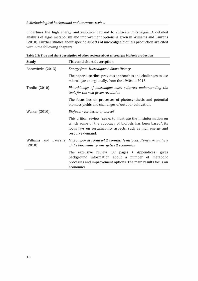
Four recent reviews on microalgae biofuels production (Table 2.3) show the challenges of future development and emphasise the need to thoroughly understand the processes of microalgae growth and cultivation in order to analyse their potential improvement.
Borowitzka (2013) summarises the previous failed attempts to produce microalgae biofuels energetically (and economically) efficiently. Tredici (2010) emphasises the challenge of attaining high photosynthetic efficiencies especially outdoors. Walker (2010)
2 Methodological background and literature review
16
underlines the high energy and resource demand to cultivate microalgae. A detailed analysis of algae metabolism and improvement options is given in Williams and Laurens (2010). Further studies about specific aspects of microalgae biofuels production are cited within the following chapters.
Table 2.3: Title and short description of other reviews about microalgae biofuels production
Study Title and short description
Borowitzka (2013) Energy from Microalgae: A Short History
The paper describes previous approaches and challenges to use microalgae energetically, from the 1940s to 2013.
Tredici (2010) Photobiology of microalgae mass cultures: understanding the tools for the next green revolution
The focus lies on processes of photosynthesis and potential biomass yields and challenges of outdoor cultivation.
Walker (2010). Biofuels – for better or worse?
This critical review “seeks to illustrate the misinformation on which some of the advocacy of biofuels has been based”, its focus lays on sustainability aspects, such as high energy and resource demand.
Williams and Laurens (2010)
Microalgae as biodiesel & biomass feedstocks: Review & analysis of the biochemistry, energetics & economics
The extensive review (37 pages + Appendices) gives background information about a number of metabolic processes and improvement options. The main results focus on economics.
17
3 Background to model microalgae growth, cultivation and biofuel production
This chapter gives the scientific background information which is necessary for understanding and thus modelling microalgae growth, cultivation and biofuels production.
Section 3.1 explains microalgae growth and its limitations, the implications of photosynthetic efficiency and the interaction of environmental conditions with microalgae growth. Section 3.2 introduces purpose and characteristics of photobioreactors, equations to calculate operation energy and further requirements to cultivate microalgae on large scale. Section 3.3 describes how biofuels can be made from microalgae, focussing on biomethane as biofuel with a low energy demand for production.
3.1 Microalgae growth
Microalgae are very small organisms (in size of a few micrometres) doing photosynthesis; they use solar energy to grow. Apart from this common feature, they are surprisingly distinct: Most belong to eukaryotes (like plants) but some are bacteria (e.g. cyanobacteria). They have manifold colours (blue, green, red, yellow) and forms and can live in all kinds of environments (Madigan et al. 2006). Algae can build their biomass from CO2 as inorganic carbon source (autotrophic growth), organic substances (heterotrophic) or both (mixotrophic). This study investigates autotrophic algae growth which requires a CO2 source.
Microalgae cultivated for energetic use have in common that they live in the water, do photosynthesis and grow by cell division. This section explains the basic principles and requirements of those mechanisms.
3.1.1 Basic mechanisms
Like any living organism, microalgae need (metabolic) energy to grow, move etc. In the following, the processes of photosynthesis and microalgae growth are explained.
3 Background to model microalgae growth, cultivation and biofuel production
18
Light reactions Dark reactions
Photosynthesis
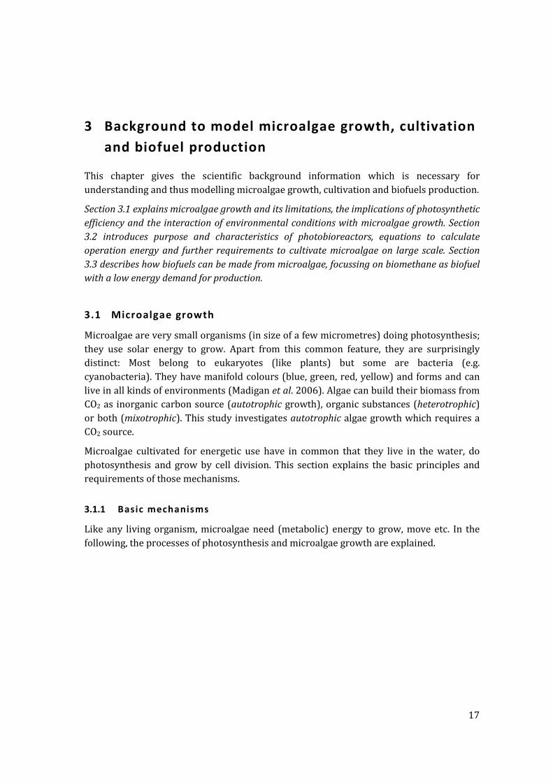
In photosynthesis, light sensitive pigments in microalgae, the chlorophylls, (part of the photosystem) absorb light energy (photons). With this energy, the molecular bonds of water (H-O-H) are split. With the evolving protons (H+) and electrons (e-) the cell builds two important functional molecules: adenosine triphosphate (ATP), the ‘fuel’ of molecular reactions, and the so called reduction equivalents (e.g. NADPH/H+) which are needed to reduce other molecules (e.g. CO2). The remaining O molecules form molecular oxygen (O2). Since photons are needed for these processes, they are called light reactions.
The cell uses the ATP and reduction equivalents (in the following called ‘metabolic energy’) from the light reactions to reduce (or ‘fix’) CO2 and assemble it to small sugar molecules in the so called Calvin Cycle (Madigan et al. 2006). Those processes do not require light and thus are called light-independent or dark reactions.
The dark reactions required to fix carbon and form biomass are orders of magnitude more slowly than the light reactions and thus limit microalgae growth (Goldman 1979, Kamen 1963).
Figure 3.1 shows the principle of photon use and electron flow in photosynthesis and the simplified light and dark reactions.
4 photons
4 photons
Photosystem II
Photosystem I
Dark reactions Light reactions
2 H2O O2 + 4H+ + 4e-
4e- + 4H+ + CO2 CH2O + H2O
2 H2O + CO2 CH2O + O2 +H2O
Further biomass production8 photons
Figure 3.1: Scheme of photosynthesis (adapted from Walker 1992)
3.1 Microalgae growth
19
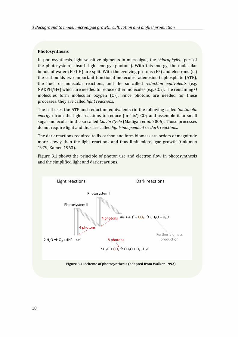
After photosynthesis: more dark reactions
With the initial small carbohydrates from photosynthesis, microalgae build larger carbohydrates, lipids and proteins. To build these molecules, microalgae require also nitrogen (N), phosphorous (P), oxygen (O), sulphur (S) and small amounts of trace elements, (e.g. iron, copper). The cell must take up all substances (in addition to CO2) from the culture medium. This requires reduction equivalents.
With those ‘building blocks’ microalgae construct complex macromolecules (DNA, enzymes) and from those again new cell structures like membranes or other cell compounds (Figure 3.2). Before a cell can replicate, it must coordinate about 2000 biochemical reactions (Madigan et al. 2006). The scheme of biomass production is schematically shown in Figure 3.2.
When a cell has enough biomass to build another cell, it divides into two (‘cell division’) and the process starts again in each cell. All processes for biomass production are in the following summarised with the term ‘growth’.
Macromolecules (enzymes, DNA…)
+ N, P, S, …
Cell structures (membranes, nukleus…)
Micromolecules(proteins, lipids, carbohydrates)
New cells (cell division)
Biomass production
Small carbohydrates from phototosynthesis
Solar energy
repe
titio
n
CO2
Figure 3.2: Scheme of biomass production in microalgae
3 Background to model microalgae growth, cultivation and biofuel production
20
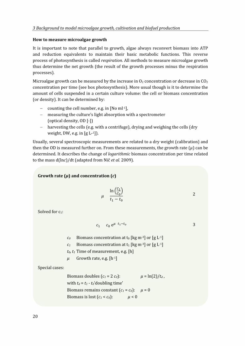
How to measure microalgae growth
It is important to note that parallel to growth, algae always reconvert biomass into ATP and reduction equivalents to maintain their basic metabolic functions. This reverse process of photosynthesis is called respiration. All methods to measure microalgae growth thus determine the net growth (the result of the growth processes minus the respiration processes).
Microalgae growth can be measured by the increase in O2 concentration or decrease in CO2 concentration per time (see box photosynthesis). More usual though is it to determine the amount of cells suspended in a certain culture volume: the cell or biomass concentration (or density). It can be determined by:
− counting the cell number, e.g. in [No ml-1], − measuring the culture’s light absorption with a spectrometer
(optical density, OD [-]) − harvesting the cells (e.g. with a centrifuge), drying and weighing the cells (dry
weight, DW, e.g. in [g L-1]).
Usually, several spectroscopic measurements are related to a dry weight (calibration) and then the OD is measured further on. From these measurements, the growth rate (µ) can be determined. It describes the change of logarithmic biomass concentration per time related to the mass d(lnc)/dt (adapted from Nič et al. 2009).
Growth rate (µ) and concentration (c)
𝜇 =ln �𝑐1
𝑐0�
𝑡1 − 𝑡0 (2)
Solved for c1:
𝑐1 = 𝑐0 e𝜇 (𝑡1−𝑡𝑜) (3)
c0 Biomass concentration at t0 [kg m-3] or [g L-1] c1 Biomass concentration at t1 [kg m-3] or [g L-1] t0, t1 Time of measurement, e.g. [h] µ Growth rate, e.g. [h-1]
Special cases:
Biomass doubles (c1 = 2 c0): µ = ln(2)/td , with td = t1 - t0‘doubling time’ Biomass remains constant (c1 = c0): µ = 0 Biomass is lost (c1 < c0): µ < 0
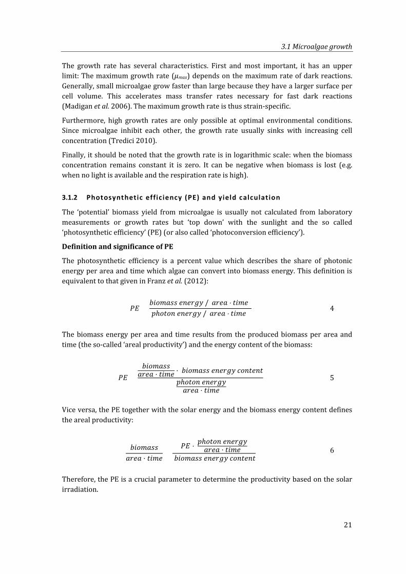
3.1 Microalgae growth
21
The growth rate has several characteristics. First and most important, it has an upper limit: The maximum growth rate (µmax) depends on the maximum rate of dark reactions. Generally, small microalgae grow faster than large because they have a larger surface per cell volume. This accelerates mass transfer rates necessary for fast dark reactions (Madigan et al. 2006). The maximum growth rate is thus strain-specific.
Furthermore, high growth rates are only possible at optimal environmental conditions. Since microalgae inhibit each other, the growth rate usually sinks with increasing cell concentration (Tredici 2010).
Finally, it should be noted that the growth rate is in logarithmic scale: when the biomass concentration remains constant it is zero. It can be negative when biomass is lost (e.g. when no light is available and the respiration rate is high).
3.1.2 Photosynthetic effic iency (PE) and yield calculation
The ‘potential’ biomass yield from microalgae is usually not calculated from laboratory measurements or growth rates but ‘top down’ with the sunlight and the so called ‘photosynthetic efficiency’ (PE) (or also called ‘photoconversion efficiency’).
Definition and significance of PE
The photosynthetic efficiency is a percent value which describes the share of photonic energy per area and time which algae can convert into biomass energy. This definition is equivalent to that given in Franz et al. (2012):
𝑃𝑁 =𝑏𝑏𝑏𝑏𝑏𝑏𝑏 𝑒𝑛𝑒𝑒𝑒𝑒 /(𝑏𝑒𝑒𝑏 ⋅ 𝑡𝑏𝑏𝑒)𝑝ℎ𝑏𝑡𝑏𝑛 𝑒𝑛𝑒𝑒𝑒𝑒 /(𝑏𝑒𝑒𝑏 ⋅ 𝑡𝑏𝑏𝑒)
(4)
The biomass energy per area and time results from the produced biomass per area and time (the so-called ‘areal productivity’) and the energy content of the biomass:
𝑃𝑁 =𝑏𝑏𝑏𝑏𝑏𝑏𝑏
𝑏𝑒𝑒𝑏 ⋅ 𝑡𝑏𝑏𝑒 ⋅ 𝑏𝑏𝑏𝑏𝑏𝑏𝑏 𝑒𝑛𝑒𝑒𝑒𝑒 𝑐𝑏𝑛𝑡𝑒𝑛𝑡
𝑝ℎ𝑏𝑡𝑏𝑛 𝑒𝑛𝑒𝑒𝑒𝑒𝑏𝑒𝑒𝑏 ⋅ 𝑡𝑏𝑏𝑒
(5)
Vice versa, the PE together with the solar energy and the biomass energy content defines the areal productivity:
𝑏𝑏𝑏𝑏𝑏𝑏𝑏𝑏𝑒𝑒𝑏 ⋅ 𝑡𝑏𝑏𝑒
=𝑃𝑁 ⋅ 𝑝ℎ𝑏𝑡𝑏𝑛 𝑒𝑛𝑒𝑒𝑒𝑒
𝑏𝑒𝑒𝑏 ⋅ 𝑡𝑏𝑏𝑒 𝑏𝑏𝑏𝑏𝑏𝑏𝑏 𝑒𝑛𝑒𝑒𝑒𝑒 𝑐𝑏𝑛𝑡𝑒𝑛𝑡
(6)
Therefore, the PE is a crucial parameter to determine the productivity based on the solar irradiation.
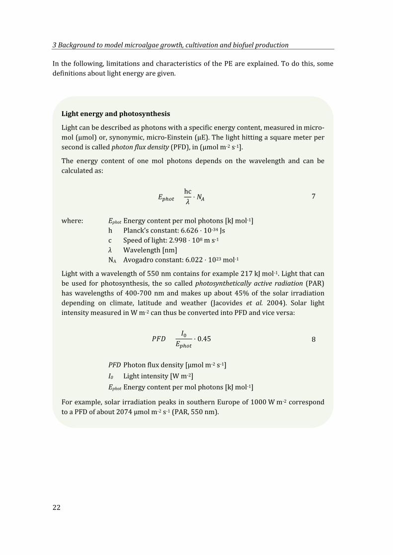
3 Background to model microalgae growth, cultivation and biofuel production
22
In the following, limitations and characteristics of the PE are explained. To do this, some definitions about light energy are given.
Light energy and photosynthesis
Light can be described as photons with a specific energy content, measured in micro-mol (µmol) or, synonymic, micro-Einstein (µE). The light hitting a square meter per second is called photon flux density (PFD), in (µmol m-2 s-1].
The energy content of one mol photons depends on the wavelength and can be calculated as:
𝑁𝑝ℎ𝑜𝑡 =hc𝜆
⋅ 𝑁𝐴 (7)
where: Ephot Energy content per mol photons [kJ mol-1] h Planck’s constant: 6.626 ⋅ 10-34 Js c Speed of light: 2.998 ⋅ 108 m s-1
λ Wavelength [nm] NA Avogadro constant: 6.022 ⋅ 1023 mol-1
Light with a wavelength of 550 nm contains for example 217 kJ mol-1. Light that can be used for photosynthesis, the so called photosynthetically active radiation (PAR) has wavelengths of 400-700 nm and makes up about 45% of the solar irradiation depending on climate, latitude and weather (Jacovides et al. 2004). Solar light intensity measured in W m-2 can thus be converted into PFD and vice versa:
𝑃𝑃𝐶 =𝐼0
𝑁𝑝ℎ𝑜𝑡⋅ 0.45 (8)
PFD Photon flux density [µmol m-2 s-1] I0 Light intensity [W m-2] Ephot Energy content per mol photons [kJ mol-1]
For example, solar irradiation peaks in southern Europe of 1000 W m-2 correspond to a PFD of about 2074 µmol m-2 s-1 (PAR, 550 nm).
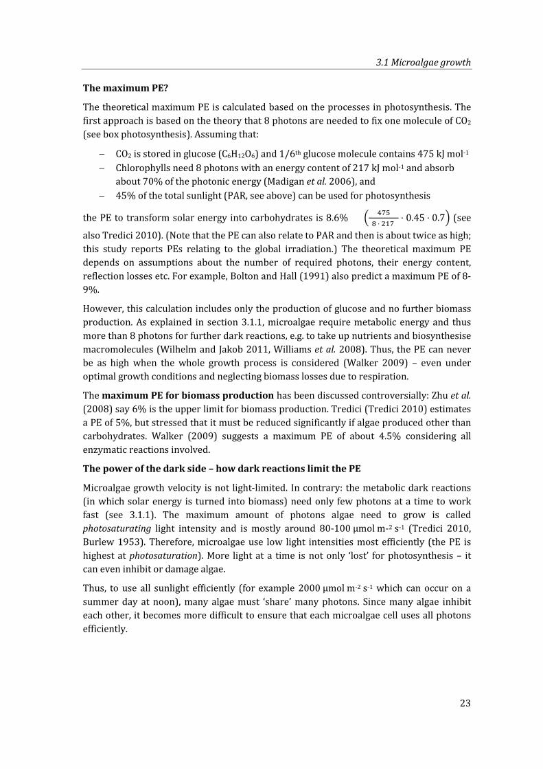
3.1 Microalgae growth
23
The maximum PE?
The theoretical maximum PE is calculated based on the processes in photosynthesis. The first approach is based on the theory that 8 photons are needed to fix one molecule of CO2 (see box photosynthesis). Assuming that:
− CO2 is stored in glucose (C6H12O6) and 1/6th glucose molecule contains 475 kJ mol-1 − Chlorophylls need 8 photons with an energy content of 217 kJ mol-1 and absorb
about 70% of the photonic energy (Madigan et al. 2006), and − 45% of the total sunlight (PAR, see above) can be used for photosynthesis
the PE to transform solar energy into carbohydrates is 8.6% = � 475(8 ⋅ 217)
⋅ 0.45 ⋅ 0.7� (see
also Tredici 2010). (Note that the PE can also relate to PAR and then is about twice as high; this study reports PEs relating to the global irradiation.) The theoretical maximum PE depends on assumptions about the number of required photons, their energy content, reflection losses etc. For example, Bolton and Hall (1991) also predict a maximum PE of 8-9%.
However, this calculation includes only the production of glucose and no further biomass production. As explained in section 3.1.1, microalgae require metabolic energy and thus more than 8 photons for further dark reactions, e.g. to take up nutrients and biosynthesise macromolecules (Wilhelm and Jakob 2011, Williams et al. 2008). Thus, the PE can never be as high when the whole growth process is considered (Walker 2009) – even under optimal growth conditions and neglecting biomass losses due to respiration.
The maximum PE for biomass production has been discussed controversially: Zhu et al. (2008) say 6% is the upper limit for biomass production. Tredici (Tredici 2010) estimates a PE of 5%, but stressed that it must be reduced significantly if algae produced other than carbohydrates. Walker (2009) suggests a maximum PE of about 4.5% considering all enzymatic reactions involved.
The power of the dark side – how dark reactions limit the PE
Microalgae growth velocity is not light-limited. In contrary: the metabolic dark reactions (in which solar energy is turned into biomass) need only few photons at a time to work fast (see 3.1.1). The maximum amount of photons algae need to grow is called photosaturating light intensity and is mostly around 80-100 µmol m-2 s-1 (Tredici 2010, Burlew 1953). Therefore, microalgae use low light intensities most efficiently (the PE is highest at photosaturation). More light at a time is not only ‘lost’ for photosynthesis – it can even inhibit or damage algae.
Thus, to use all sunlight efficiently (for example 2000 µmol m-2 s-1 which can occur on a summer day at noon), many algae must ‘share’ many photons. Since many algae inhibit each other, it becomes more difficult to ensure that each microalgae cell uses all photons efficiently.
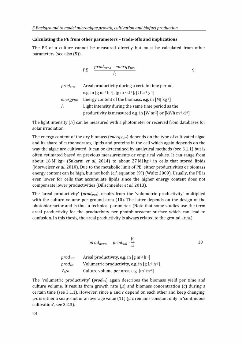
3 Background to model microalgae growth, cultivation and biofuel production
24
Calculating the PE from other parameters – trade-offs and implications
The PE of a culture cannot be measured directly but must be calculated from other parameters (see also (5)).
𝑃𝑁 =𝑝𝑒𝑏𝑝𝑔𝑐𝑐𝑔 ⋅ 𝑒𝑛𝑒𝑒𝑒𝑒𝐷𝐷
𝐼0 (9)
prodarea Areal productivity during a certain time period, e.g. in [g m-2 h-1], [g m-2 d-1], [t ha-1 y-1] energyDW Energy content of the biomass, e.g. in [MJ kg-1] I0 Light intensity during the same time period as the productivity is measured e.g. in [W m-2] or [kWh m-2 d-1]
The light intensity (I0) can be measured with a photometer or received from databases for solar irradiation.
The energy content of the dry biomass (energyDW) depends on the type of cultivated algae and its share of carbohydrates, lipids and proteins in the cell which again depends on the way the algae are cultivated. It can be determined by analytical methods (see 3.1.1) but is often estimated based on previous measurements or empirical values. It can range from about 16 MJ kg-1 (Sukarni et al. 2014) to about 27 MJ kg-1 in cells that stored lipids (Morweiser et al. 2010). Due to the metabolic limit of PE, either productivities or biomass energy content can be high, but not both (c.f. equation (9)) (Waltz 2009). Usually, the PE is even lower for cells that accumulate lipids since the higher energy content does not compensate lower productivities (Dillschneider et al. 2013).
The ‘areal productivity’ (prodarea) results from the ‘volumetric productivity’ multiplied with the culture volume per ground area (10). The latter depends on the design of the photobioreactor and is thus a technical parameter. (Note that some studies use the term areal productivity for the productivity per photobioreactor surface which can lead to confusion. In this thesis, the areal productivity is always related to the ground area.)
𝑝𝑒𝑏𝑝𝑔𝑐𝑐𝑔 = 𝑝𝑒𝑏𝑝𝑣𝑜𝑓 ⋅𝑉𝑐
𝑏 (10)
prodarea Areal productivity, e.g. in [g m-2 h-1] prodvol Volumetric productivity, e.g. in [g L-1 h-1] Vc/a Culture volume per area, e.g. [m3 m-2]
The ‘volumetric productivity’ (prodvol) again describes the biomass yield per time and culture volume. It results from growth rate (µ) and biomass concentration (c) during a certain time (see 3.1.1). However, since µ and c depend on each other and keep changing, µ⋅c is either a snap-shot or an average value (11) (µ⋅c remains constant only in ‘continuous cultivation’, see 3.2.3).
3.1 Microalgae growth
25
𝑝𝑒𝑏𝑝𝑣𝑜𝑓 = µ𝑐��� (11)
µ𝑐��� Product of growth rate and cell concentration (average)
This method to calculate the PE from laboratory measurements is also defined in (Hu and Richmond 1996). With the above definitions, the PE can be expressed as ((10)and (11) in (9)):
𝑃𝑁 =µ𝑐��� ⋅ 𝑉𝑐
𝑏 ⋅ 𝑒𝑛𝑒𝑒𝑒𝑒𝐷𝐷
𝐼0 (12)
In summary, the PE has the following characteristics:
− The PE is related to the growth rate and thus depends in the same way on environmental conditions (e.g. temperature, mass transfer rates) as the growth rate.
− High PEs are not equivalent to high areal productivities. On the contrary: the PE is usually high at low light intensities – then productivities are low.
− The PE can relate to different time scales. By rearranging equation (9), areal productivities can be calculated vice versa from the PE, light intensity and energy content of the biomass:
𝑝𝑒𝑏𝑝𝑔𝑐𝑐𝑔 =𝑃𝑁 ⋅ 𝐼0
𝑒𝑛𝑒𝑒𝑒𝑒𝐷𝐷 (13)
To calculate the areal productivity, it is crucial to consider that the PE is linked to the conditions under which it is attained. For example, calculating the ‘potential’ maximum productivity from a maximum PE and the yearly irradiation (such as in Stephens et al. 2010) implies that optimal growth conditions are provided during the whole year.
3.1.3 Good and bad growth conditions
Microalgae need specific optimal conditions to grow fast – and thus attain high PE (turn photons efficiently into biomass). This section introduces the requirements for good growth conditions and the mechanisms responsible for growth inhibition and low PE.
Good growth conditions – and how they are usually provided
a) Enough light: mixing
Most algae need only around 80-100 µmol m-2 s-1 (photosaturating light intensity) to fuel their dark reactions (Tredici 2010, Burlew 1953). Outdoors, the light intensity is mostly much higher. Thus, light does not limit microalgae growth – unless algae shade each other. In their natural environments algae usually do not accumulate above a few mg L-1 and do

3 Background to model microalgae growth, cultivation and biofuel production
26
not shade each other significantly. Shading is indeed a problem in algae mass cultivation which aims for concentrations above several g L-1. Tredici (2010) showed that a culture of 4 g L-1 absorbs almost all light within 6 mm. Therefore, cultures are mixed to bring each cell to the illuminated surface regularly.
It has been proposed that algae can ‘harvest’ very high light intensities in a short time and use them efficiently in complete darkness (‘flashing light effect’). This must happen in well-defined periods of milliseconds; wrong cycle lengths have an adverse effect (Lehr 2012, Burlew 1953).
b) Concentrated CO2: gassing
Algae can grow using CO2 from the air (0.4 vol%) – but not fast. To make algae grow fast, concentrated CO2 must be supplied to the culture. CO2 supply is often coupled with O2 removal since the O2 produced in the light reaction inhibits photosynthesis. Gasses can be exchanged in various ways: within the PBR or using external devices; for an overview see (Carvalho et al. 2006). In aerated PBRs, the culture is sparged with CO2 (pure or mixed with air). Aeration can also be used to mix the culture since the rising gas bubbles move the culture medium.
c) High mass transfer rates: mixing
Algae must be able to take up nutrients and CO2 fast. Mixing distributes substances in the culture and removes boundary layers around the cells and thus enhances mass transfer rates (Hu and Richmond 1996, Grobbelaar 1994). Turbulence can be provoked by aeration (see above) or by pumping the culture medium through the reactor.
d) Optimal enzymatic reactions: temperature, pH and salt concentration
The numerous enzymes catalysing the dark reactions function well only within a very narrow range of temperature, pH and salt concentration (Figure 3.3), the respective optimal conditions depend on the algae strain. Thus, in order to attain high PE, the culture medium must provide optimal conditions at any time.
Rate
of e
nzym
e ac
tivity
pH or temperature Figure 3.3: How enzyme activity depends on pH or temperature (qualitatively)
3.1 Microalgae growth
27
Bad growth conditions
When growth conditions are not optimal, algae grow more slowly or not at all, they can even loose biomass or die. In any case, the PE sinks. Adverse conditions and the underlying mechanisms are explained as follows:
e) Not enough light: photolimitation and respiration
Without enough light (photolimitation) algae grow slowly or even loose biomass when the respiration rate is higher than the growth rate. The faster algae grow, the more they respirate. Therefore, much biomass is lost when the light intensity suddenly sinks; photosynthesis stops but respiration rates remain high (Wilhelm and Jakob 2011, Kok 1953). Abrupt changes in light intensity should thus be avoided. This is a problem when algae shade each other at high biomass concentration.
f) Too much light or changing light intensities: photoprotection and photoadaption
When algae are exposed to high light intensities (above photosaturation, see above) for a longer time, they must protect their light-sensitive chlorophylls and other organs: algae reduce their chlorophyll content, build protective pigments and dissipate photonic energy as heat (Wilhelm and Selmar 2011, Perry et al. 1981). These processes take time (up to several hours) and metabolic energy.
Once adapted, algae can use also high light intensities efficiently (Tamiya et al. 1953, p. 209, Fig.3) although they still dissipate some photonic energy as heat. When the light intensity sinks again, the cell must reverse the adaptation processes: they remove protective pigments and build more chlorophyll again. High light adapted algae cannot use low light efficiently and vice versa (Tredici 2010). Irradiation outdoors can vary between complete darkness to over 2000 µmol m-2 s-1 within a few hours (see also Annex, Table A.1). Thus efficient light use is challenging outdoors.
Algae die when exposed to very high light intensities for a longer time (so-called photoinhibition). For example, the green algae Chlamydomonas reinhardtii is photoinhibited above 1600 µmol m-2 s-1 (Franz et al. 2012).
g) Too much oxygen: photorespiration
Algae produce oxygen during photosynthesis (see box photosynthesis). When many algae grow fast they build much oxygen. Oxygen can bind to – and thus inhibit – one of the major enzymes needed to fix CO2 (Ribulose-1,5-bisphosphate carboxylase/oxygenase, ‘RuBisCo’). The cells must actively detach the O2 from RuBisCo (Sousa et al. 2012, Tredici 2010). This also costs the cell metabolic energy and the PE sinks. Oxygen builds also radicals which damage the cell. For example, an inhibiting oxygen concentration (120-200% of the oxygen concentration of ambient air) can occur already after 1 min in a tube without gas exchange (Posten 2009).
h) No nutrients: storage processes
Without N and P, algae cannot build functional molecules, such as proteins (see 3.1.1) and thus cannot grow (Waltz 2009, Wykoff et al. 1998). They have to store carbohydrates in form of starch or lipids in their cell body. When nutrients are available again, algae can
3 Background to model microalgae growth, cultivation and biofuel production
28
reconvert carbohydrates to functional molecules. These processes require additional metabolic energy which consequently cannot be used for growing; the PE sinks (Wilhelm and Jakob 2012).
Microalgae intended to make biodiesel should contain many storage lipids and thus are on purpose cultivated without N or P.
i) Wrong temperature: growth inhibition or death
The temperature limits the rate of enzymatic reactions. Since those are already growth limiting, the wrong temperature limits algae growth and photon use even more than the suboptimal light intensities (Tamiya et al. 1953).
Generally, heat is much more harmful to algae than cold: While low temperatures slow down metabolic reactions, heat disintegrates functional molecules (e.g. enzymes) and algae die. For example, most algae die within less than an 30 minutes when exposed to 50°C (Agrawal and Singh 2000). Temperature management is thus crucial to cultivate microalgae.
j) Contamination and mutual inhibition
Apart from physical and chemical circumstances, other micro- or macro-organisms inhibit and damage algae. For example, most water organisms feed on algae; fungi and viruses damage algae, and bacteria compete with algae for nutrients or light. Thus it must be avoided that other organisms contaminate the culture. Contamination can be avoided by using closed photobioreactors (PBRs) or by cultivating specific algae strains at extreme pH. Some algae attach to the reactor walls and build biofilms so that cleaning is necessary (Hulatt and Thomas 2011).
In addition to that, microalgae inhibit each other in every of the above mentioned aspects: they shade each other, compete for CO2 and nutrients and excrete O2 and other growth inhibiting substances (Harris 1970).
Figure 3.4 summarises how the energy output in form of biomass qualitatively depends on the growth conditions – and thus the energy demand for cultivation. Note that high mass transfer rates are a precondition for almost all requirements to ensure fast growth.
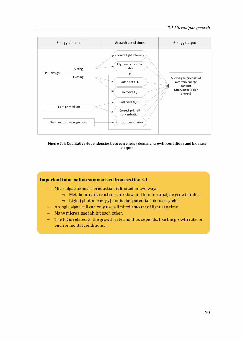
3.1 Microalgae growth
29
Temperature management
Correct light intensity
Mixing
Sufficient CO2
Culture mediumCorrect pH, salt concentration
Correct temperature
Sufficient N,P,S
Remove O2
PBR designMicroalgae biomass of
a certain energy content
(‚Harvested‘ solar energy)
Energy demand Growth conditions
High mass transfer rates
Energy output
Gassing
Figure 3.4: Qualitative dependencies between energy demand, growth conditions and biomass
output
Important information summarised from section 3.1
− Microalgae biomass production is limited in two ways: → Metabolic dark reactions are slow and limit microalgae growth rates. → Light (photon energy) limits the ‘potential’ biomass yield.
− A single algae cell can only use a limited amount of light at a time. − Many microalgae inhibit each other. − The PE is related to the growth rate and thus depends, like the growth rate, on
environmental conditions.
3 Background to model microalgae growth, cultivation and biofuel production
30
3.2 Photobioreactors and microalgae mass cultivation
Photobioreactors (PBRs) are technical systems containing the microalgae, water and nutrients. Different devices supply concentrated CO2, remove O2, and mix the culture. The purpose of PBRs is to provide good growth conditions as described in 3.1.2 and thus achieve high PE and high areal biomass productivities (Figure 3.5). In the following, options of PBR design and operation are introduced and discussed.
Biomass production
PBR operation & design
Light, heat
Photosynthetic efficiency (PE) of microalgae
Figure 3.5: Interaction of PBR operation and design, PE and biomass production
3.2.1 Photobioreactor design
Photobioreactors can be shaped in any form, e.g. like tubes, columns, flat panels, bags (floating, hanging) etc. (see for example Pruvost 2011, Tredici 2003, Pulz 2001). To provide algae with sunlight, PBRs have either transparent or no (upper) walls.
Most studies distinguish between so called ‘open (raceway) ponds’ and other photobioreactors. Open ponds resemble stirred lakes where the culture is in contact with open air; they can be dug into the ground. PBRs are closed containments of glass or plastic and are suspended from frames or aligned on the ground. Advantages and disadvantages of different systems are compared in (Ugwu et al. 2008, Tredici 2003, Tredici and Materassi 1992).
Characteristic parameters
Any cultivation system can be described with a set of parameters, including:
h Height [m] w Width [m] (also called ‘light path’) d Diameter [m] (used in tubular PBRs) l Length [m]
Those and the PBR design determine other characteristic parameters and quotients, like the culture volume Vc and the culture volume per area Vc/a.
Vc Culture volume [L] or [m3] a Land area occupied by the system [m2]
The culture volume per area is a key parameter to calculate volume-related data from area-related data and vice versa. A low culture volume per area reduces the energy
3.2 Photobioreactors and microalgae mass cultivation
31
demand per area (Morweiser et al. 2010). However, the lower the culture volume per area is, the higher must be the cell concentration to harvest all photons (see equation (12)) and the higher is the risk of overheating and oxygen accumulation. These factors have led to the breakdown of many outdoor microalgae plants (Tredici 2003, Janssen et al. 2003). Therefore the culture volume per area has a lower limit; PBRs outdoors usually contain 50 to 200 L m-2 (0.05 – 0.20 m3 m-2) (Tredici 2003); Morweiser et al. (2010) report best values of about 0.040 m3 m-2.
Figure 3.6 displays different rectangular cultivation systems and their characteristics. The volume per area depends on the design of the single cultivation system and on the distance of units to each other. For example in open ponds, the volume per area is about equivalent to the pond depth. In flat plate PBRs, it is equivalent to the reactor width (or ‘light path’) if the height equals the distance; placing vertical PBRs closer together increases the volume per area (see Figure 3.6, d) compared to e)).
a) b) c) d) e)
1 m
𝛼
Side view
Top view
Characteristics a) b) c) d) e) Open or closed open closed closed closed closed Width w [m] (or ‘light path’) 0.10 0.05 0.05 0.05 0.05 Volume per area Vc/a [m3 m-2] 0.10 0.05 0.05 0.05 0.10 Height h [m] 0.10 sin 𝛼 1.00 0.50 0.50 Captures all photons/ ground area
yes (w/o margin)
yes (w/o margin)
no no no
Figure 3.6: Different microalgae cultivation systems (side and top view) and their characteristics
3 Background to model microalgae growth, cultivation and biofuel production
32
Capturing the sunlight – orientation, temperature and light management
PBRs should capture most of the sunlight without overheating. Outdoors, the sun shines on PBRs at various angles and intensities during the day – from the side or from above (see Figure 3.6). To avoid overheating, temperature and light intensity can be controlled actively or passively.
Active temperature control – such as spray cooling or heat exchange – needs water, energy, and material depending on the type and operation mode (e.g. flow rates) (see for example Meyer and Weiss 2014).
Passive temperature control (e.g. shading with dark sheets, immersion in water, vertical position) simply avoids high light intensities – but thus also ‘loses’ the solar energy accordingly. Torzillo et al. (1986) for example reported that shading of tubular PBR with dark-coloured plastic sheets caused “a strong reduction in the amount of solar radiation received by the culture and consequently in the yield of biomass.”
Vertical PBRs for example do not capture high solar irradiation at noon (Tredici and Materassi 1992) and shade each other, especially when the sun rises and sets. The exact amount of harvested photons depends on many parameters, such as the PBR geometry, material, orientation, and distance of units, on the location (latitude and season), and on the biomass concentration and light intensity at each cultivation time (Slegers et al. 2011). A positive effect of vertical PBRs is that algae can use the diffuse and low light more efficiently than direct light (see 3.1.2). However, Hu et al. (1996) showed that at otherwise identical cultivation conditions, a 30° inclined PBR attained higher productivities than a 60° and 90°(vertical) PBR for outdoor cultivation (June and July in Israel) – higher PE could not compensate for the lost solar energy (Figure 3.7). For aerated photobioreactors, a minimum inclination is needed to ensure that the gas bubbles rise.
In general, appropriate heat and light management depends on the region or location where algae are cultivated; for example it is less challenging to avoid overheating in Norway than in Spain.
Figure 3.7: Volumetric productivity of a PBR positioned at different angles, illuminated from one
or two sides (based on data of Hu et al. 1996)
0.0
0.5
1.0
1.5
2.0
2.5
30° 60° 90°
prod
vol[
g L-1
d-1]
two sides
one side
3.2 Photobioreactors and microalgae mass cultivation
33
Material
Photobioreactors are exposed to sunlight and different weather the whole year round. Thus their material must be extremely durable and stable. Some systems are thus protected, for example they are covered by a greenhouse or immersed in water (Posten 2009).
Above that, PBR material should be transparent, non-toxic, cheap, and easy to process (Tredici 2003). Polycarbonate (PC), polyethylene (PE), polyvinylchloride (PVC), polyethylene terephthalate (PET) and glass are suggested as reactor materials (Burgess and Fernández-Velasco 2007). Most PBRs are built of glass or thin plastic foils. After use, material could be combusted or recycled to recover energy.
Material demand for PBRs depends on the PBR form and the thickness and density of the used material. For example, for a rectangular PBR, it can be calculated as:
𝑥𝑚𝑔𝑡 = ( ℎ ⋅ 𝑙 + 𝑤 ⋅ 𝑙 + 𝑤 ⋅ ℎ) ⋅ 2 ⋅ 𝜌𝑚 ⋅ 𝑡ℎ (14)
xmat Material demand [kg] ρm Density of the material [kg m-3] th Thickness of the walls [m]
To calculate material demand for more complex designs, more parameters are required.
3.2.2 Calculating the operation energy
This section introduces and shortly discusses the most important parameters and equations needed to calculate the operation energy with a focus on aeration. Aeration can be used to provide CO2, remove O2 (exchange gasses) and to mix the culture at the same time. For different methods of gas exchange in microalgae cultures see Carvalho et al. (2006). Options to reduce operation energy which are directly visible from the equations are also shortly discussed.
Aeration rate (vvm)
The aeration rate is the delivered gas volume per time (�̇�𝑔) and per culture volume Vc (15); it is often indicated per minute (vvm). The term vvm is commonly used for microalgae cultivation, and is mainly used in this study.
�̇�𝑔
𝑉𝑐 =
𝑣𝑔 ⋅ 𝐴𝑔
𝑉𝑐 (15)
�̇�𝑔
𝑉𝑐 Aeration rate (e.g. [m³gas m-3 s-1], mostly in vvm [m³gas m-3 min-1])
Vc Culture volume [m3] vg (hypothetical or superficial) gas velocity [m s-1] or [m min-1] Ag Flow cross-section gas [m2]
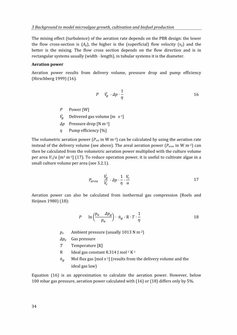
3 Background to model microalgae growth, cultivation and biofuel production
34
The mixing effect (turbulence) of the aeration rate depends on the PBR design: the lower the flow cross-section is (Ag), the higher is the (superficial) flow velocity (vg) and the better is the mixing. The flow cross section depends on the flow direction and is in rectangular systems usually (width ⋅ length), in tubular systems it is the diameter.
Aeration power
Aeration power results from delivery volume, pressure drop and pump efficiency (Hirschberg 1999) (16).
𝑃 = 𝑉�̇� ⋅ 𝛥𝑝 ⋅1𝜂
(16)
P Power [W] 𝑉�̇� Delivered gas volume [m³ s-1] Δp Pressure drop [N m-2] η Pump efficiency [%]
The volumetric aeration power (Pvol in W m-3) can be calculated by using the aeration rate instead of the delivery volume (see above). The areal aeration power (Parea in W m-2) can then be calculated from the volumetric aeration power multiplied with the culture volume per area Vc/a [m3 m-2] (17). To reduce operation power, it is useful to cultivate algae in a small culture volume per area (see 3.2.1).
𝑃𝑔𝑐𝑐𝑔 =𝑉�̇�
𝑉𝑐 ⋅ 𝛥𝑝 ⋅
1𝜂
⋅𝑉𝑐
𝑏 (17)
Aeration power can also be calculated from isothermal gas compression (Roels and Heijnen 1980) (18):
𝑃 = ln �𝑝𝑔 + 𝛥𝑝𝑔
𝑝𝑔� ⋅ �̇�𝑔 ⋅ R ⋅ 𝑇 ⋅
1𝜂
(18)
pa Ambient pressure (usually 1013 N m-2) Δpg Gas pressure T Temperature [K] R Ideal gas constant 8.314 J mol-1 K-1 �̇�𝑔 Mol flux gas [mol s-1] (results from the delivery volume and the ideal gas law)
Equation (16) is an approximation to calculate the aeration power. However, below 100 mbar gas pressure, aeration power calculated with (16) or (18) differs only by 5%.
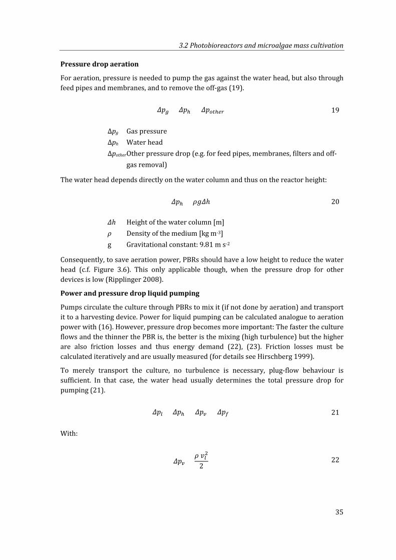
3.2 Photobioreactors and microalgae mass cultivation
35
Pressure drop aeration
For aeration, pressure is needed to pump the gas against the water head, but also through feed pipes and membranes, and to remove the off-gas (19).
𝛥𝑝𝑔 = 𝛥𝑝ℎ + 𝛥𝑝𝑜𝑡ℎ𝑐𝑐 (19)
Δpg Gas pressure Δph Water head Δpother Other pressure drop (e.g. for feed pipes, membranes, filters and off- gas removal)
The water head depends directly on the water column and thus on the reactor height:
𝛥𝑝ℎ = 𝜌𝑒𝛥ℎ (20)
Δh Height of the water column [m] ρ Density of the medium [kg m-3] g Gravitational constant: 9.81 m s-2
Consequently, to save aeration power, PBRs should have a low height to reduce the water head (c.f. Figure 3.6). This only applicable though, when the pressure drop for other devices is low (Ripplinger 2008).
Power and pressure drop liquid pumping
Pumps circulate the culture through PBRs to mix it (if not done by aeration) and transport it to a harvesting device. Power for liquid pumping can be calculated analogue to aeration power with (16). However, pressure drop becomes more important: The faster the culture flows and the thinner the PBR is, the better is the mixing (high turbulence) but the higher are also friction losses and thus energy demand (22), (23). Friction losses must be calculated iteratively and are usually measured (for details see Hirschberg 1999).
To merely transport the culture, no turbulence is necessary, plug-flow behaviour is sufficient. In that case, the water head usually determines the total pressure drop for pumping (21).
𝛥𝑝𝑓 = 𝛥𝑝ℎ + 𝛥𝑝𝑣 + 𝛥𝑝𝑓 (21)
With:
𝛥𝑝𝑣 =𝜌 𝑣𝑓
2
2 (22)
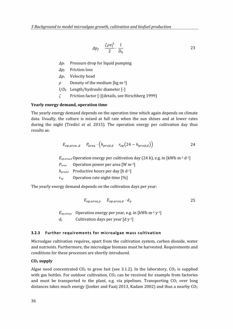
3 Background to model microalgae growth, cultivation and biofuel production
36
𝛥𝑝𝑓 =𝜁𝜌𝑣𝑓
2
2⋅
l𝐶ℎ
(23)
Δpl Pressure drop for liquid pumping Δpf Friction loss Δpv Velocity head ρ Density of the medium [kg m-3] l/Dh Length/hydraulic diameter [-] ζ Friction factor [-](details, see Hirschberg 1999)
Yearly energy demand, operation time
The yearly energy demand depends on the operation time which again depends on climate data. Usually, the culture is mixed at full rate when the sun shines and at lower rates during the night (Tredici et al. 2015). The operation energy per cultivation day thus results as:
𝑁𝑜𝑝,𝑔𝑐𝑐𝑔 ,𝑐 = 𝑃𝑔𝑐𝑐𝑔 ⋅ �ℎ𝑝𝑐𝑜𝑐,𝑐 + 𝑒𝑜𝑝�24 − ℎ𝑝𝑐𝑜𝑐,𝑐�� (24)
Eop.area,d Operation energy per cultivation day (24 h), e.g. in [kWh m-2 d-1] Parea Operation power per area [W m-2] hprod,d Productive hours per day [h d-1] rop Operation rate night-time [%]
The yearly energy demand depends on the cultivation days per year:
𝑁𝑜𝑝,𝑔𝑐𝑐𝑔,𝑦 = 𝑁𝑜𝑝,𝑔𝑐𝑐𝑔,𝑐 ⋅ 𝑝𝑦 (25)
Eop,area,y Operation energy per year, e.g. in [kWh m-2 y-1] dy Cultivation days per year [d y-1]
3.2.3 Further requirements for microalgae mass cultivation
Microalgae cultivation requires, apart from the cultivation system, carbon dioxide, water and nutrients. Furthermore, the microalgae biomass must be harvested. Requirements and conditions for these processes are shortly introduced.
CO2 supply
Algae need concentrated CO2 to grow fast (see 3.1.2). In the laboratory, CO2 is supplied with gas bottles. For outdoor cultivation, CO2 can be received for example from factories and must be transported to the plant, e.g. via pipelines. Transporting CO2 over long distances takes much energy (Jonker and Faaij 2013, Kadam 2002) and thus a nearby CO2
3.2 Photobioreactors and microalgae mass cultivation
37
source is favourable. These places are very limited though. The distance to the next CO2 source considerably limits the potential of microalgae cultivation (Skarka 2015).
The less efficient algae take up CO2, the more must be transported to the culture. Doucha et al. (2005) for example measured 50% CO2 uptake in an open thin layer PBR. CO2 uptake is better in closed PBRs. Rate and amount of CO2 absorption depends on the type of gassing, but also on the CO2 concentration in the gas and the quality of mixing and mass transfer (Carvalho and Malcata 2001).
Nutrients and water
Apart from a carbon source, algae need nutrients such as nitrogen and phosphorous and further micronutrients (see 3.1.1). In the laboratory, the culture medium is sterilised and the nutrient mixture is optimised for each algae strain (Hu et al. 1996). This is not applicable for mass cultivation. For large scale microalgae cultivation, it is suggested to add fertiliser, such as used to cultivate crops, to the culture. The culture medium must contain more nutrients than algae consist of to ensure that algae can take them up.
To save fertiliser, some studies suggest cultivating algae in wastewater (Mu et al. 2014). Wastewater use is not assessed in this study for the following reasons: Wastewater has changing pH and salt concentrations, is often turbid and contains other microorganisms or growth inhibiting substances. Potential lower yields and/or pre-treatment of wastewater thus can offset fertiliser savings (Razon and Tan 2011). Besides, wastewater is usually available in urban areas where cheap and unused land is scarce (Fortier and Sturm 2012, Lundquist et al. 2010).
To use natural water sources and avoid transportation, the cultivation plant must be located near the coast or the shore of a lake respectively. Alternatively, groundwater could be used which must be pumped up.
Harvesting
Microalgae are extremely small. Consequently, much energy is required to separate them from the water. Usually, the culture is pumped to a harvesting device which separates the cells from the water with filters or shear forces (e.g. centrifuge). For a review of several harvesting options see Rawat et al. (2013).
To pre-concentrate cultures, they can be pumped into a pond and left there for a few hours or days so that algae settle on the ground. The residual water is removed. Chemicals (so called flocculants, e.g. salts of multivalent cations) can be added to the culture so that microalgae agglomerate and sink faster (Bilanovic et al. 1988). Flocculants can however inhibit other chemical processes needed to obtain a biofuel.
The biomass must be harvested in certain intervals, e.g. after a defined time period or when the culture reaches a certain concentration. Three different operation/harvesting modes can be distinguished:
− In so called ‘batches’, the whole biomass in a PBR is harvested. Fresh cells, e.g. from another PBR are used to inoculate a new culture medium.
3 Background to model microalgae growth, cultivation and biofuel production
38
− In ‘semi-batch’ or ‘semi-continuous’ cultivation only a part of the biomass is harvested. The remaining culture is filled up with fresh medium. Outdoor cultures are usually operated that way. The share of biomass which is needed to inoculate the next culture (and thus cannot be harvested) depends on the operation mode, cell concentration and growth rate.
− In ‘continuous cultivation’, newly grown biomass is being constantly harvested and fresh medium is constantly added at the same rate. (The dilution rate* must be equal to the growth rate). By this means the biomass concentration [g L-1] is held constant. Continuous cultivation is the ‘high art’ of cultivating microorganisms and usually only possible in the laboratory under highly controlled conditions. *The dilution rate is reciprocal to the average time a particle (e.g. a single algae cell) or volume element of the culture stays in a bioreactor (hydraulic retention time, HRT) (Nič et al. 2009).
The harvesting method also determines biomass losses at night due to respiration: When most of the biomass is harvested, the starting concentration is low the next day. This results in low productivities, even at maximum growth rates (see definition of growth rate 3.1.1). On the other hand, high biomass concentrations overnight result in high respiration losses. Thus, a balance must be found between harvesting and respiration losses.
Harvesting energy is, like operation energy, usually related to a volume (e.g. kWh m-3). For batch or semi-batch cultivation, the yearly harvesting energy depends on the culture volume and how often it is exchanged:
𝑁ℎ𝑔𝑐𝑣,𝑦 = 𝑁ℎ𝑔𝑐𝑣,𝑣𝑜𝑓 ⋅ 𝑉𝑐,𝑦 (26)
Eharv,vol Harvesting energy per culture volume, e.g. in [kWh m-3] Vc,y Culture volume per year [m3 y-1]
The latter depends on the cultivation time per year and the batch length:
𝑉𝑐,𝑦 = 𝑉𝑐 ⋅ 𝑝𝑦
𝑝𝑐𝑒 (27)
dex Batch length, days between culture exchange
Energy for culture transport (filling and emptying the PBRs) is analogue:
𝑁𝑡𝑐,𝑦 = 𝑁𝑡𝑐,𝑣𝑜𝑓 ⋅ 𝑉𝑐,𝑦 ⋅ 2 (28)
Etr,vol Pump energy per culture volume, e.g. in [kWh m-3]
3.3 Microalgae biofuels production
39
3.3 Microalgae biofuels production
This section shortly introduces how different biofuels can be made from microalgae biomass with a focus on biomethane as a benchmark for the net energy ratio.
3.3.1 Different fuels
Microalgae contain proteins, carbohydrates and lipids in different shares depending on the microalgae strain and the way it is cultivated. Thus, algae biomass can be turned into a variety of fuels, such as (bio-) ethanol, diesel or hydrogen or methane.
The most investigated fuel is biodiesel. To produce it, algae are cultivated without nutrients so that they store lipids (see 3.1.2). These lipids are extracted from the (dried) biomass, saturated and purified. Each process step can be done in different ways and thus almost an unlimited number of biofuels and process combinations can be examined. For an overview of some, see for example (Aitken and Antizar-Ladislao 2012, Khoo et al. 2011, Sander and Murthy 2010, Williams and Laurens 2010, Sialve et al. 2009).
To produce biohydrogen, specific algae and cultivation conditions are required: The green algae Chlamydomonas reinhardtii can digest its own biomass into hydrogen under anaerobic conditions and without sulphur (Hallenbeck and Benemann 2002).
Biomethane production is energetically ‘cheap’
The focus of this study is set on biomethane production from the algae biomass because it requires the least efforts both during biomass production and downstream processing:
− For biomethane production, algae do not need to store lipids or produce other special substances; they only need to grow fast. This results in higher growth rates (Rodolfi et al. 2009) and photosynthetic efficiencies (Wilhelm and Jakob 2012).
− The wet biomass can directly be put into the biogas plant. It is not necessary to previously dry it or to extract substances – those processes costs very much energy. Sills et al. (2012) showed that drying as well as wet lipid extraction consumed more energy than is stored in the fuel (1.8 and 1.6 MJ MJ-1 respectively) (see also Woertz et al. 2014, Lardon et al. 2009, Sander and Murthy 2010, Khoo et al. 2011, Dassey et al. 2014).
Important information summarised from section 3.2
− Good growth conditions depend on PBR operation and design. − The aeration rate determines the quality of gas exchange and mixing and is
directly proportional to the operation energy.
3 Background to model microalgae growth, cultivation and biofuel production
40
Thus, biomethane production from microalgae biomass is investigated in this study. Already in 1959, Golueke and Oswald proposed the fermentation of microalgae biomass to produce methane (Borowitzka 2013).
Note that microalgae biofuels production is not economically feasible yet, either (Woertz et al. 2014). Thus, economically, it would make more sense to produce non-energetic high value products (HVP, for example vitamins, antioxidants, colorants etc.) with microalgae, as already done today.
Biofuels as a by-product? Methodological considerations
It has repeatedly been suggested to produce high value products (HVP) and biofuels from the same biomass. A ‘coupled’ production is not assessed in this dissertation for several reasons (see also 1.3).
First of all, very few microalgae products generate residues and thus the potential of biofuels as a by-product is marginal. Moreover methodological issues must be considered about how to calculate environmental burdens of a system with several outputs (Klöpffer and Grahl 2009). There are mainly two options:
a) Bioenergy and HVP are considered to be equivalent products. This can be dealt with so called ‘allocation’ and ‘substitution’ methods.
− Allocation (energetic): The cumulative energy demand (CED) of the whole production chain is distributed between the products according to their energy content. Since HVP do not contain much energy, this accounts the major part of the energy demand to the biofuel. (Other allocation criteria are mass or prices, however it is compulsory to use ‘energetic allocation’ for assessing energy products (European Parliament and European Council 2009)).
− Substitution: If the HVP from microalgae substitutes another substance, the biofuel can receive a credit for the ‘avoided’ energy to produce the respective other substance. This can lead to a wide range of credits depending on the substitute. ISO norms on LCA recommend the application of different substitution and allocation methods to assess how the results depend on the method.
However, ‘equivalent’ production is rather hypothetical: the HVP is usually the main product of microalgae cultivation since it can be sold for higher prices.
b) Bioenergy is considered to be made from the ‘waste’ or residuals of HVP
Wastes are defined to have zero life cycle emissions. The fact that waste can be used energetically should not lead to producing more waste. This is paradox is also a problem for other fuels from waste.
For the above named reasons, the NER is calculated for microalgae biomethane as the main and only product.
3.3 Microalgae biofuels production
41
3.3.2 Biomethane production
To produce biomethane, biomass (the substrate) is mixed with anaerobic bacteria and heated for a certain time until the bacteria degraded most parts via hydrolysis and acidogenesis of the biomass into methane (CH4), carbon dioxide (CO2) and few other gasses (Deublein and Steinhauser 2011). The methane is then separated from other gasses and purified.
The type of substrate determines whether the fermentation processes is dry or wet, what temperature is needed, and whether it is operated (semi-)continuously or in batches (see also 3.2.2). Microalgae biomass can be fermented wet; for this, the ferment should contain 2-10% dry weigth (DW). Wet fermentation usually is done in batches of 15 to 32 days (Deublein and Steinhauser 2011).
The fermenting bacteria need about 1 nitrogen (N) molecule per 20-30 carbon (C) molecules (C/N-ratio of 20-30). More nitrogen reacts with hydrogen to ammonia which inhibits methane production. With less nitrogen, the digesting bacteria cannot form proteins (analogue to microalgae growth c.f. 3.1.2). Since most microalgae have a lower C/N-ratio than required, they should be co-digested, e.g. with maize (Sialve et al. 2009).
The biomethane yield per kg volatile substance (VS, the digestible part of microalgae) depends on the type of microalgae and the operation mode (Mussgnug et al. 2010). Experiments showed biomethane yields between 0.18 and 0.39 Nm3 (normal cubic metre) per kg substrate for different microalgae species (Mussgnug et al. 2010); with lower values when biomass is dried previously. For further details about biomethane production, see (Meyer 2012, Deublein and Steinhauser 2011).
Important information summarised from section 3.3
− Microalgae can be turned into a variety of fuels. The type of biofuel depends on the algae strain, the growth conditions and type of downstream processing.
− The most energy efficient fuel is biomethane since it does not require lipid accumulation and needs least downstream energy.
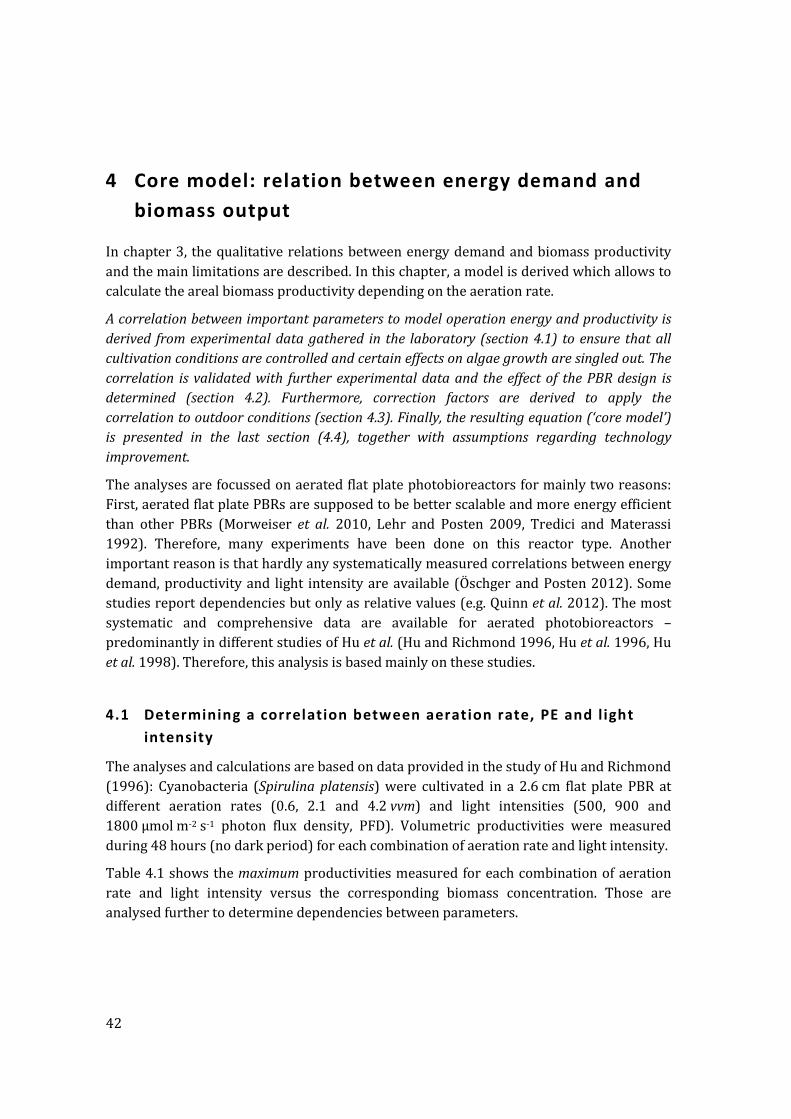
42
4 Core model: relation between energy demand and biomass output
In chapter 3, the qualitative relations between energy demand and biomass productivity and the main limitations are described. In this chapter, a model is derived which allows to calculate the areal biomass productivity depending on the aeration rate.
A correlation between important parameters to model operation energy and productivity is derived from experimental data gathered in the laboratory (section 4.1) to ensure that all cultivation conditions are controlled and certain effects on algae growth are singled out. The correlation is validated with further experimental data and the effect of the PBR design is determined (section 4.2). Furthermore, correction factors are derived to apply the correlation to outdoor conditions (section 4.3). Finally, the resulting equation (‘core model’) is presented in the last section (4.4), together with assumptions regarding technology improvement.
The analyses are focussed on aerated flat plate photobioreactors for mainly two reasons: First, aerated flat plate PBRs are supposed to be better scalable and more energy efficient than other PBRs (Morweiser et al. 2010, Lehr and Posten 2009, Tredici and Materassi 1992). Therefore, many experiments have been done on this reactor type. Another important reason is that hardly any systematically measured correlations between energy demand, productivity and light intensity are available (Öschger and Posten 2012). Some studies report dependencies but only as relative values (e.g. Quinn et al. 2012). The most systematic and comprehensive data are available for aerated photobioreactors – predominantly in different studies of Hu et al. (Hu and Richmond 1996, Hu et al. 1996, Hu et al. 1998). Therefore, this analysis is based mainly on these studies.
4.1 Determining a correlation between aeration rate, PE and l ight intensity
The analyses and calculations are based on data provided in the study of Hu and Richmond (1996): Cyanobacteria (Spirulina platensis) were cultivated in a 2.6 cm flat plate PBR at different aeration rates (0.6, 2.1 and 4.2 vvm) and light intensities (500, 900 and 1800 µmol m-2 s-1 photon flux density, PFD). Volumetric productivities were measured during 48 hours (no dark period) for each combination of aeration rate and light intensity.
Table 4.1 shows the maximum productivities measured for each combination of aeration rate and light intensity versus the corresponding biomass concentration. Those are analysed further to determine dependencies between parameters.
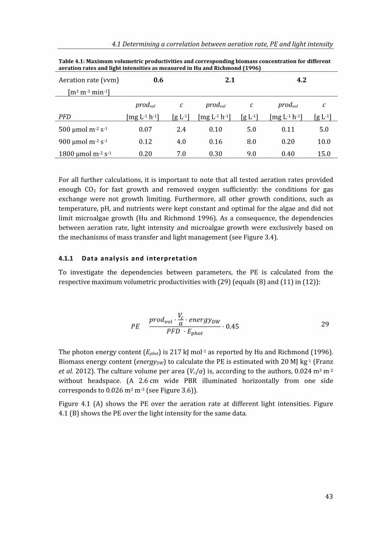
4.1 Determining a correlation between aeration rate, PE and light intensity
43
Table 4.1: Maximum volumetric productivities and corresponding biomass concentration for different aeration rates and light intensities as measured in Hu and Richmond (1996)
Aeration rate (vvm)
[m3 m-3 min-1]
0.6 2.1 4.2
prodvol c prodvol c prodvol c
PFD [mg L-1 h-1] [g L-1] [mg L-1 h-1] [g L-1] [mg L-1 h-1] [g L-1]
500 µmol m-2 s-1 0.07 2.4 0.10 5.0 0.11 5.0
900 µmol m-2 s-1 0.12 4.0 0.16 8.0 0.20 10.0
1800 µmol m-2 s-1 0.20 7.0 0.30 9.0 0.40 15.0
For all further calculations, it is important to note that all tested aeration rates provided enough CO2 for fast growth and removed oxygen sufficiently: the conditions for gas exchange were not growth limiting. Furthermore, all other growth conditions, such as temperature, pH, and nutrients were kept constant and optimal for the algae and did not limit microalgae growth (Hu and Richmond 1996). As a consequence, the dependencies between aeration rate, light intensity and microalgae growth were exclusively based on the mechanisms of mass transfer and light management (see Figure 3.4).
4.1.1 Data analysis and interpretation
To investigate the dependencies between parameters, the PE is calculated from the respective maximum volumetric productivities with (29) (equals (8) and (11) in (12)):
𝑃𝑁 =𝑝𝑒𝑏𝑝𝑣𝑜𝑓 ⋅ 𝑉𝑐
𝑏 ⋅ 𝑒𝑛𝑒𝑒𝑒𝑒𝐷𝐷
𝑃𝑃𝐶 ⋅ 𝑁𝑝ℎ𝑜𝑡⋅ 0.45 (29)
The photon energy content (Ephot) is 217 kJ mol-1 as reported by Hu and Richmond (1996). Biomass energy content (energyDW) to calculate the PE is estimated with 20 MJ kg-1 (Franz et al. 2012). The culture volume per area (Vc/a) is, according to the authors, 0.024 m3 m-2 without headspace. (A 2.6 cm wide PBR illuminated horizontally from one side corresponds to 0.026 m3 m-3 (see Figure 3.6)).
Figure 4.1 (A) shows the PE over the aeration rate at different light intensities. Figure 4.1 (B) shows the PE over the light intensity for the same data.
4 Core model: relation between energy demand and biomass output
44
Figure 4.1: Dependencies between PE, aeration rate and light intensity: (A) PE over aeration rate,
(B) PE over light intensity, based on data of Hu and Richmond (1996)
Figure 4.1 (A) clearly shows that the PE depends on the aeration rate. More interestingly, the correlation is non-linear: while the PE doubles in the best case (from 3% to 6% at 1800 µmol m-2 s-1) the aeration rate increases sevenfold (from 0.6 to 4.2 vvm). Much more energy is needed to attain high PE (and thus a high biomass energy output) than low. Furthermore, it can be seen that at low aeration rates, the PE depends additionally on the light intensity (Figure 4.1 B).
0.0%
1.0%
2.0%
3.0%
4.0%
5.0%
6.0%
7.0%
0 1 2 3 4 5
Phot
osyn
thet
ic e
ffici
ency
(PE)
[%
]
Aeration rate (vvm) [m3 m-3 min-1]
500
900
1800
0.0%
1.0%
2.0%
3.0%
4.0%
5.0%
6.0%
7.0%
0 500 1000 1500 2000
Phot
osyn
thet
ic e
ffici
ency
(PE)
[%]
Light intensity (I0) [µmol m-2 s-1]
4.2 vvm
2.1 vvm
0.6 vvm
A µmol m-2 s-1
µmol m-2 s-1
µmol m-2 s-1
B
PFD
4.1 Determining a correlation between aeration rate, PE and light intensity
45
These data confirm the theoretical background explained in chapter 3: High PE at high light intensities requires a high biomass concentration (see Table 4.1 and equation (12)). Since algae shade and inhibit each other, it becomes more difficult to attain high PE. Consequently, higher aeration rates (and thus more energy) are required to ensure that the individual cell:
− maintains high mass transfer rates needed for fast dark reactions and − receives enough light but not too much (avoid photolimitation and
photoinhibition).
Whether one or the other effect is responsible for the positive effect of mixing has been discussed controversially: Posten (2009) emphasises that high mass transfer rates are at least equally important as good light management. This can be seen also from Figure 3.4. Grobbelaar (1994) finds that a combination of light-dark cycles and mass transfer rates explain the positive effect of mixing; while Ugwu (2008) suggest that it is mainly the high mass transfer rates.
With the assumed energy content of 20 MJ kgDW-1, the maximum PE is around 6% (Figure 4.1 A and B). The authors’ suggestion of Spirulina biomass energy content of 22.4 MJ kgDW-1 resulted in even higher PE of around 7% (c.f. equation (12)). Nevertheless, a PE of 6% is the upper limit expected for biomass production (see 3.1.2). The PE could have come close to the theoretical maximum because (a) cyanobacteria are small and fast-growing (Madigan et al. 2006) and (b) had optimal growth conditions (temperature, nutrients, constant light intensities, see Figure 3.4). Therefore, the energy content of 20 MJ kgDW-1 is used further on.
4.1.2 Areal energy balance and ‘core energy ratio’
To further analyse the data of Hu and Richmond (1996), the areal operation energy is compared to the areal biomass energy output (areal energy balance). The quotient of these values is defined in this study as ‘core energy ratio’ (CER) (30). This presentation has two advantages:
First, it is easier to compare different studies based on these values. Data about operation energy and productivities are generally better available than PE or aeration rates. Second, the quotient already gives a first indication of the NER since it includes the parameters which mainly determine the NER. The NER is always higher than the CER since it includes further upstream and downstream energy demand. Areal energy balance and CER can also be calculated for other time units.
𝐶𝑁𝑁 = 𝑁𝑜𝑝,𝑔𝑐𝑐𝑔,𝑐
𝑁𝑏𝑏𝑜𝑚,𝑔𝑐𝑐𝑔,𝑐 (30)
Eop,area,d Operation energy input per area and day [Wh m-2 d-1] Ebiom,area,d Biomass energy output per area and day [Wh m-2 d-1]
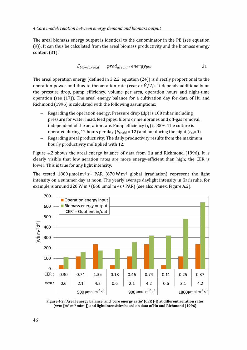
4 Core model: relation between energy demand and biomass output
46
The areal biomass energy output is identical to the denominator in the PE (see equation (9)). It can thus be calculated from the areal biomass productivity and the biomass energy content (31):
𝑁𝑏𝑏𝑜𝑚,𝑔𝑐𝑐𝑔,𝑐 = 𝑝𝑒𝑏𝑝𝑔𝑐𝑐𝑔,𝑐 ⋅ 𝑒𝑛𝑒𝑒𝑒𝑒𝐷𝐷 (31)
The areal operation energy (defined in 3.2.2, equation (24)) is directly proportional to the operation power and thus to the aeration rate (vvm or �̇�/Vc). It depends additionally on the pressure drop, pump efficiency, volume per area, operation hours and night-time operation (see (17)). The areal energy balance for a cultivation day for data of Hu and Richmond (1996) is calculated with the following assumptions:
− Regarding the operation energy: Pressure drop (Δp) is 100 mbar including pressure for water head, feed pipes, filters or membranes and off-gas removal, independent of the aeration rate. Pump efficiency (η) is 85%. The culture is operated during 12 hours per day (hprod,d = 12) and not during the night (rop=0).
− Regarding areal productivity: The daily productivity results from the maximum hourly productivity multiplied with 12.
Figure 4.2 shows the areal energy balance of data from Hu and Richmond (1996). It is clearly visible that low aeration rates are more energy-efficient than high; the CER is lower. This is true for any light intensity.
The tested 1800 µmol m-2 s-1 PAR (870 W m-2 global irradiation) represent the light intensity on a summer day at noon. The yearly average daylight intensity in Karlsruhe, for example is around 320 W m-2 (660 µmol m-2 s-1 PAR) (see also Annex, Figure A.2).
Figure 4.2: ‘Areal energy balance’ and ‘core energy ratio’ (CER [-]) at different aeration rates
(vvm [m3 m-3 min-1]) and light intensities based on data of Hu and Richmond (1996)
0.30 0.74 1.35 0.18 0.46 0.74 0.11 0.25 0.370
100
200
300
400
500
600
700
0.6 2.1 4.2 0.6 2.1 4.2 0.6 2.1 4.2
500 900 1800
[Wh
m-2
d-1]
Operation energy inputBiomass energy output'CER' = Quotient in/out
µmol m-2 s-1
vvm :
CER :
µmol m-2 s-1 µmol m-2 s-1
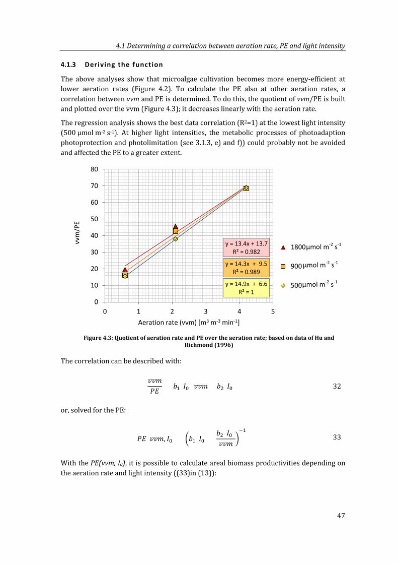
4.1 Determining a correlation between aeration rate, PE and light intensity
47
4.1.3 Deriving the function
The above analyses show that microalgae cultivation becomes more energy-efficient at lower aeration rates (Figure 4.2). To calculate the PE also at other aeration rates, a correlation between vvm and PE is determined. To do this, the quotient of vvm/PE is built and plotted over the vvm (Figure 4.3); it decreases linearly with the aeration rate.
The regression analysis shows the best data correlation (R2=1) at the lowest light intensity (500 µmol m-2 s-1). At higher light intensities, the metabolic processes of photoadaption photoprotection and photolimitation (see 3.1.3, e) and f)) could probably not be avoided and affected the PE to a greater extent.
Figure 4.3: Quotient of aeration rate and PE over the aeration rate; based on data of Hu and
Richmond (1996)
The correlation can be described with:
𝑣𝑣𝑏𝑃𝑁
= 𝑏1(𝐼0) 𝑣𝑣𝑏 + 𝑏2(𝐼0) (32)
or, solved for the PE:
𝑃𝑁(𝑣𝑣𝑏, 𝐼0) = �𝑏1(𝐼0) +𝑏2(𝐼0)𝑣𝑣𝑏
�−1
(33)
With the PE(vvm, I0), it is possible to calculate areal biomass productivities depending on the aeration rate and light intensity ((33)in (13)):
y = 13.4x + 13.7R² = 0.982
y = 14.3x + 9.5R² = 0.989
y = 14.9x + 6.6R² = 1
0
10
20
30
40
50
60
70
80
0 1 2 3 4 5
vvm
/PE
Aeration rate (vvm) [m3 m-3 min-1]
1800
900
500
µmol m-2 s-1
µmol m-2 s-1
µmol m-2 s-1
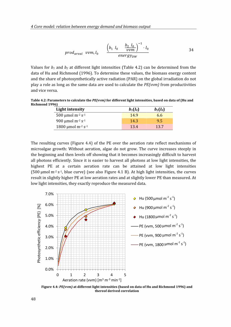
4 Core model: relation between energy demand and biomass output
48
𝑝𝑒𝑏𝑝𝑔𝑐𝑐𝑔𝑓 (𝑣𝑣𝑏, 𝐼0) =�𝑏1(𝐼0) + 𝑏2(𝐼0)
𝑣𝑣𝑏 �−1
⋅ 𝐼0
𝑒𝑛𝑒𝑒𝑒𝑒𝐷𝐷 (34)
Values for b1 and b2 at different light intensities (Table 4.2) can be determined from the data of Hu and Richmond (1996). To determine these values, the biomass energy content and the share of photosynthetically active radiation (PAR) on the global irradiation do not play a role as long as the same data are used to calculate the PE(vvm) from productivities and vice versa.
Table 4.2: Parameters to calculate the PE(vvm) for different light intensities, based on data of (Hu and Richmond 1996)
Light intensity b1(I0) b2(I0) 500 µmol m-2 s-1 14.9 6.6 900 µmol m-2 s-1 14.3 9.5 1800 µmol m-2 s-1 13.4 13.7
The resulting curves (Figure 4.4) of the PE over the aeration rate reflect mechanisms of microalgae growth: Without aeration, algae do not grow. The curve increases steeply in the beginning and then levels off showing that it becomes increasingly difficult to harvest all photons efficiently. Since it is easier to harvest all photons at low light intensities, the highest PE at a certain aeration rate can be attained at low light intensities (500 µmol m-2 s-1, blue curve) (see also Figure 4.1 B). At high light intensities, the curves result in slightly higher PE at low aeration rates and at slightly lower PE than measured. At low light intensities, they exactly reproduce the measured data.
Figure 4.4: PE(vvm) at different light intensities (based on data of Hu and Richmond 1996) and
thereof derived correlation
0.0%
1.0%
2.0%
3.0%
4.0%
5.0%
6.0%
7.0%
0 1 2 3 4 5
Phot
osyn
thet
ic e
ffici
ency
(PE)
[%
]
Aeration rate (vvm) [m3 m-3 min-1]
Hu (500
Hu (900
Hu (1800
PE (vvm, 500
PE (vvm, 900
PE (vvm, 1800
µmol m-2 s-1)
µmol m-2 s-1)
µmol m-2 s-1)
µmol m-2 s-1)
µmol m-2 s-1)
µmol m-2 s-1)
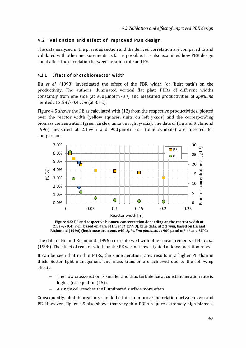
4.2 Validation and effect of improved PBR design
49
4.2 Validation and effect of improved PBR design
The data analysed in the previous section and the derived correlation are compared to and validated with other measurements as far as possible. It is also examined how PBR design could affect the correlation between aeration rate and PE.
4.2.1 Effect of photobioreactor width
Hu et al. (1998) investigated the effect of the PBR width (or ‘light path’) on the productivity. The authors illuminated vertical flat plate PBRs of different widths constantly from one side (at 900 µmol m-2 s-1) and measured productivities of Spirulina aerated at 2.5 +/- 0.4 vvm (at 35°C).
Figure 4.5 shows the PE as calculated with (12) from the respective productivities, plotted over the reactor width (yellow squares, units on left y-axis) and the corresponding biomass concentration (green circles, units on right y-axis). The data of (Hu and Richmond 1996) measured at 2.1 vvm and 900 µmol m-2 s-1 (blue symbols) are inserted for comparison.
Figure 4.5: PE and respective biomass concentration depending on the reactor width at
2.5 (+/- 0.4) vvm, based on data of Hu et al. (1998); blue data: at 2.1 vvm, based on Hu and Richmond (1996) (both measurements with Spirulina platensis at 900 µmol m-2 s-1 and 35°C)
The data of Hu and Richmond (1996) correlate well with other measurements of Hu et al. (1998). The effect of reactor width on the PE was not investigated at lower aeration rates.
It can be seen that in thin PBRs, the same aeration rates results in a higher PE than in thick. Better light management and mass transfer are achieved due to the following effects:
− The flow cross-section is smaller and thus turbulence at constant aeration rate is higher (c.f. equation (15)).
− A single cell reaches the illuminated surface more often.
Consequently, photobioreactors should be thin to improve the relation between vvm and PE. However, Figure 4.5 also shows that very thin PBRs require extremely high biomass
0
5
10
15
20
25
30
0.0%
1.0%
2.0%
3.0%
4.0%
5.0%
6.0%
7.0%
0 0.05 0.1 0.15 0.2 0.25
Biom
ass c
once
ntra
tion
c [
g L-1
]
PE [%
]
Reactor width [m]
PEc
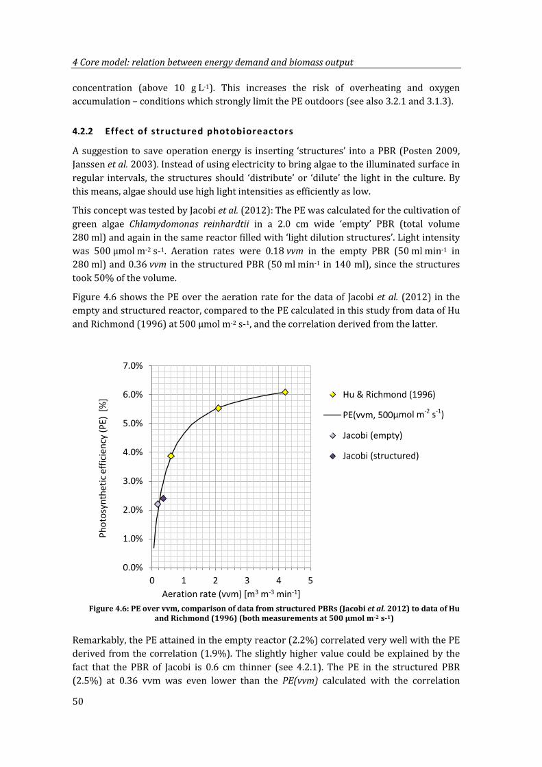
4 Core model: relation between energy demand and biomass output
50
concentration (above 10 g L-1). This increases the risk of overheating and oxygen accumulation – conditions which strongly limit the PE outdoors (see also 3.2.1 and 3.1.3).
4.2.2 Effect of structured photobioreactors
A suggestion to save operation energy is inserting ‘structures’ into a PBR (Posten 2009, Janssen et al. 2003). Instead of using electricity to bring algae to the illuminated surface in regular intervals, the structures should ‘distribute’ or ‘dilute’ the light in the culture. By this means, algae should use high light intensities as efficiently as low.
This concept was tested by Jacobi et al. (2012): The PE was calculated for the cultivation of green algae Chlamydomonas reinhardtii in a 2.0 cm wide ‘empty’ PBR (total volume 280 ml) and again in the same reactor filled with ‘light dilution structures’. Light intensity was 500 µmol m-2 s-1. Aeration rates were 0.18 vvm in the empty PBR (50 ml min-1 in 280 ml) and 0.36 vvm in the structured PBR (50 ml min-1 in 140 ml), since the structures took 50% of the volume.
Figure 4.6 shows the PE over the aeration rate for the data of Jacobi et al. (2012) in the empty and structured reactor, compared to the PE calculated in this study from data of Hu and Richmond (1996) at 500 µmol m-2 s-1, and the correlation derived from the latter.
Figure 4.6: PE over vvm, comparison of data from structured PBRs (Jacobi et al. 2012) to data of Hu
and Richmond (1996) (both measurements at 500 µmol m-2 s-1)
Remarkably, the PE attained in the empty reactor (2.2%) correlated very well with the PE derived from the correlation (1.9%). The slightly higher value could be explained by the fact that the PBR of Jacobi is 0.6 cm thinner (see 4.2.1). The PE in the structured PBR (2.5%) at 0.36 vvm was even lower than the PE(vvm) calculated with the correlation
0.0%
1.0%
2.0%
3.0%
4.0%
5.0%
6.0%
7.0%
0 1 2 3 4 5
Phot
osyn
thet
ic e
ffici
ency
(PE)
[%
]
Aeration rate (vvm) [m3 m-3 min-1]
Hu & Richmond (1996)
PE(vvm, 500
Jacobi (empty)
Jacobi (structured)
µmol m-2 s-1)
4.3 Effects of outdoor mass cultivation
51
(3.0%). One reason for this could be that the structures inhibited aeration induced mass transfer. Another reason could be the different growth behaviour of the green algae Chlamydomonas compared to the cyanobacteria Spirulina.
The authors expected higher PE at high light intensities due to the structures, this was not tested though. However, a high PE at high light intensities requires also higher biomass concentration (see equation (12) and 4.2.1). Biomass concentration was below 1 g L-1 in this experiment.
In summary, the correlation between vvm and PE is derived from data of a thin (2.6 cm wide) PBR and thus is optimistic. Data measured in other experiments confirm the correlation.
4.3 Effects of outdoor mass cultivation
The correlation derived in section 4.1.3 is based on laboratory measurements. Outdoors, temperature and light intensity keep changing; biomass is lost due to night-time respiration, harvesting, or even fouling or predators (see 3.1.3). To consider the respective aspects, correction factors are determined to apply the correlation to outdoor mass cultivation. The correction factors can be multiplied with the PE, the solar irradiation or the areal productivity since all parameters result from each other (see equation (13)).
4.3.1 Temperature correction
The interaction of temperature and microalgae growth (see 3.1.3 i) can be considered in three ways:
a) The temperature of the culture is not regulated; suboptimal temperatures decrease algae growth and thus the PE (Franz et al. 2012).
b) The culture temperature is controlled passively (e.g. by shading) and consequently a share of the solar energy is lost (see 3.2.1).
c) The culture temperature is actively regulated (e.g. by heat exchange or spray cooling) which requires energy.
Modelling the energy demand for temperature regulation (approach c) is beyond the scope of this work. For the other approaches, temperature correction factors are derived:
To model approach a), the temperature correction factor changes hourly according to the difference between the actual temperature and the optimal growth temperature of the strain. The respective correction factor is derived from a distribution function, as described in Franz et al. (2012). Irradiation and temperature at each cultivation hour are derived from climate data. Those are obtained exemplarily for a location in southern Germany (Karlsruhe) and southern Europe (Madrid) for the year 2012 (Huld 2013, Huld et al. 2012, example shown in Annex, Table A.1).
To model approach b), a constant correction factor is determined, representing photon losses due to passive temperature control.
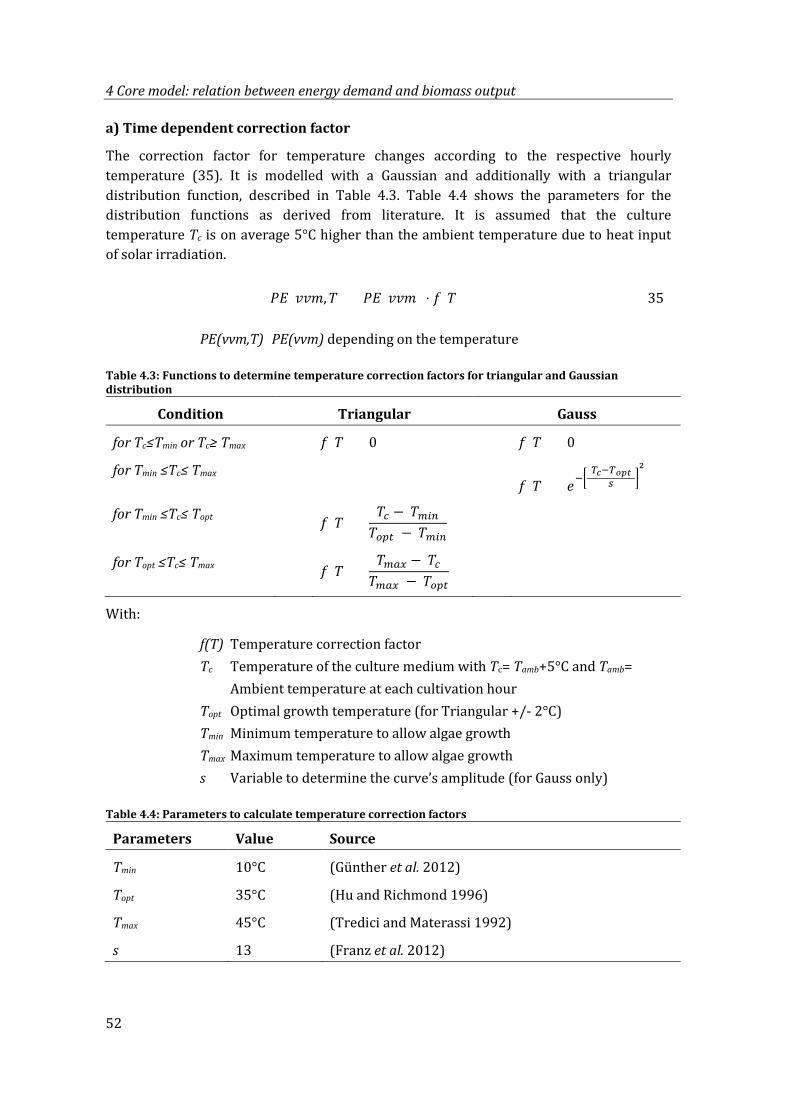
4 Core model: relation between energy demand and biomass output
52
a) Time dependent correction factor
The correction factor for temperature changes according to the respective hourly temperature (35). It is modelled with a Gaussian and additionally with a triangular distribution function, described in Table 4.3. Table 4.4 shows the parameters for the distribution functions as derived from literature. It is assumed that the culture temperature Tc is on average 5°C higher than the ambient temperature due to heat input of solar irradiation.
𝑃𝑁(𝑣𝑣𝑏, 𝑇) = 𝑃𝑁(𝑣𝑣𝑏) ⋅ 𝑓(𝑇) (35)
PE(vvm,T) PE(vvm) depending on the temperature
Table 4.3: Functions to determine temperature correction factors for triangular and Gaussian distribution
Condition Triangular Gauss
for Tc≤Tmin or Tc≥ Tmax 𝑓(𝑇) = 0 𝑓(𝑇) = 0
for Tmin ≤Tc≤ Tmax 𝑓(𝑇) = 𝑒−�
(𝑇𝑐−𝑇𝑜𝑜𝑜)𝑔 �
2
for Tmin ≤Tc≤ Topt 𝑓(𝑇) =𝑇𝑐 − 𝑇𝑚𝑏𝑛
𝑇𝑜𝑝𝑡 − 𝑇𝑚𝑏𝑛
for Topt ≤Tc≤ Tmax 𝑓(𝑇) =𝑇𝑚𝑔𝑒 − 𝑇𝑐
𝑇𝑚𝑔𝑒 − 𝑇𝑜𝑝𝑡
With:
f(T) Temperature correction factor Tc Temperature of the culture medium with Tc= Tamb+5°C and Tamb= Ambient temperature at each cultivation hour Topt Optimal growth temperature (for Triangular +/- 2°C) Tmin Minimum temperature to allow algae growth Tmax Maximum temperature to allow algae growth s Variable to determine the curve’s amplitude (for Gauss only)
Table 4.4: Parameters to calculate temperature correction factors
Parameters Value Source
Tmin 10°C (Günther et al. 2012)
Topt 35°C (Hu and Richmond 1996)
Tmax 45°C (Tredici and Materassi 1992)
s 13 (Franz et al. 2012)
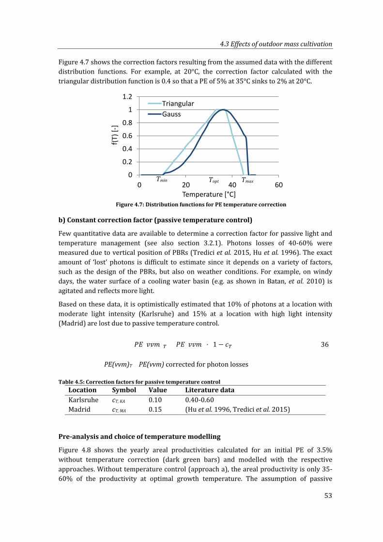
4.3 Effects of outdoor mass cultivation
53
Figure 4.7 shows the correction factors resulting from the assumed data with the different distribution functions. For example, at 20°C, the correction factor calculated with the triangular distribution function is 0.4 so that a PE of 5% at 35°C sinks to 2% at 20°C.
Figure 4.7: Distribution functions for PE temperature correction
b) Constant correction factor (passive temperature control)
Few quantitative data are available to determine a correction factor for passive light and temperature management (see also section 3.2.1). Photons losses of 40-60% were measured due to vertical position of PBRs (Tredici et al. 2015, Hu et al. 1996). The exact amount of ‘lost’ photons is difficult to estimate since it depends on a variety of factors, such as the design of the PBRs, but also on weather conditions. For example, on windy days, the water surface of a cooling water basin (e.g. as shown in Batan, et al. 2010) is agitated and reflects more light.
Based on these data, it is optimistically estimated that 10% of photons at a location with moderate light intensity (Karlsruhe) and 15% at a location with high light intensity (Madrid) are lost due to passive temperature control.
𝑃𝑁(𝑣𝑣𝑏)𝑇 = 𝑃𝑁(𝑣𝑣𝑏) ⋅ (1 − 𝑐𝑇) (36)
PE(vvm)T PE(vvm) corrected for photon losses
Table 4.5: Correction factors for passive temperature control Location Symbol Value Literature data Karlsruhe cT, KA 0.10 0.40-0.60
(Hu et al. 1996, Tredici et al. 2015) Madrid cT, MA 0.15
Pre-analysis and choice of temperature modelling
Figure 4.8 shows the yearly areal productivities calculated for an initial PE of 3.5% without temperature correction (dark green bars) and modelled with the respective approaches. Without temperature control (approach a), the areal productivity is only 35-60% of the productivity at optimal growth temperature. The assumption of passive
0
0.2
0.4
0.6
0.8
1
1.2
0 20 40 60
f(T) [
-]
Temperature [°C]
TriangularGauss
Tmin Topt Tmax
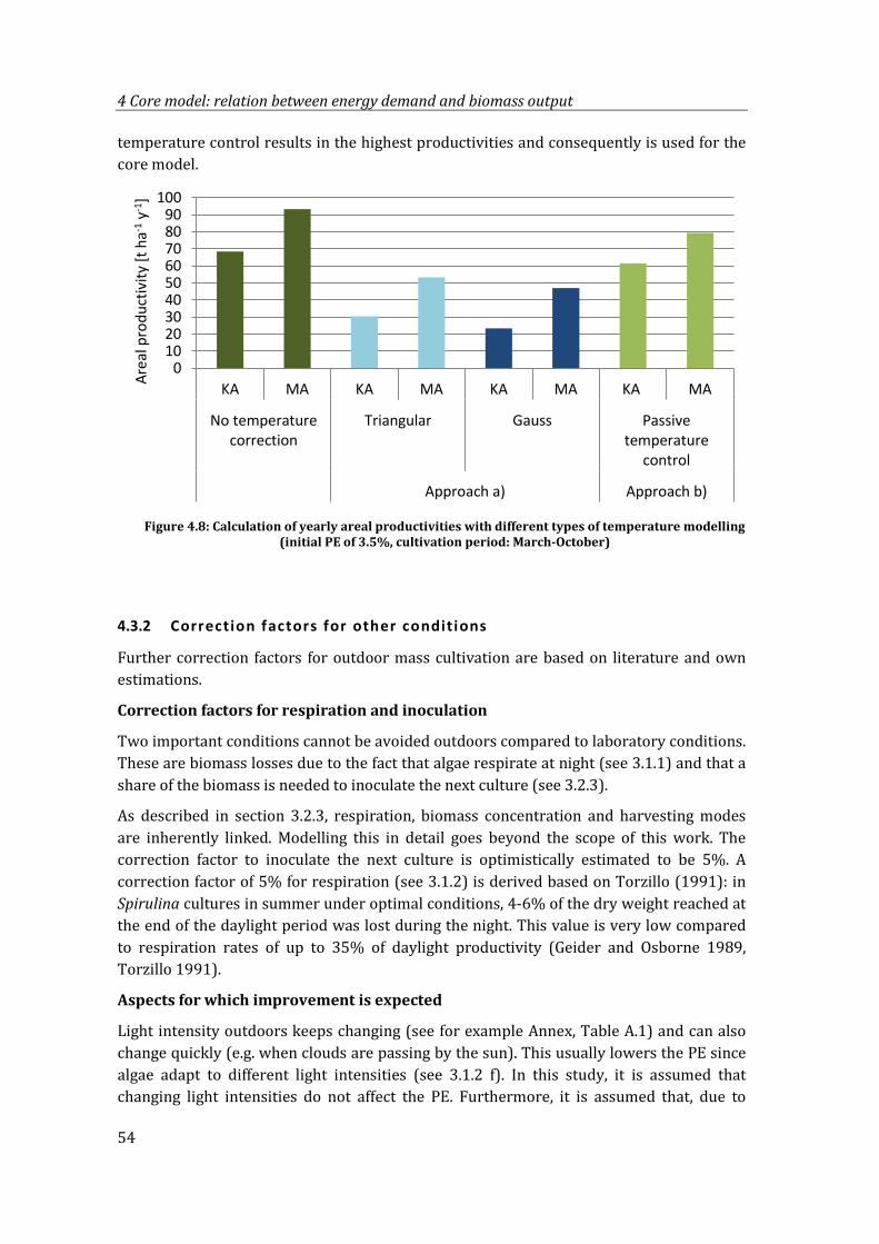
4 Core model: relation between energy demand and biomass output
54
temperature control results in the highest productivities and consequently is used for the core model.
Figure 4.8: Calculation of yearly areal productivities with different types of temperature modelling
(initial PE of 3.5%, cultivation period: March-October)
4.3.2 Correction factors for other conditions
Further correction factors for outdoor mass cultivation are based on literature and own estimations.
Correction factors for respiration and inoculation
Two important conditions cannot be avoided outdoors compared to laboratory conditions. These are biomass losses due to the fact that algae respirate at night (see 3.1.1) and that a share of the biomass is needed to inoculate the next culture (see 3.2.3).
As described in section 3.2.3, respiration, biomass concentration and harvesting modes are inherently linked. Modelling this in detail goes beyond the scope of this work. The correction factor to inoculate the next culture is optimistically estimated to be 5%. A correction factor of 5% for respiration (see 3.1.2) is derived based on Torzillo (1991): in Spirulina cultures in summer under optimal conditions, 4-6% of the dry weight reached at the end of the daylight period was lost during the night. This value is very low compared to respiration rates of up to 35% of daylight productivity (Geider and Osborne 1989, Torzillo 1991).
Aspects for which improvement is expected
Light intensity outdoors keeps changing (see for example Annex, Table A.1) and can also change quickly (e.g. when clouds are passing by the sun). This usually lowers the PE since algae adapt to different light intensities (see 3.1.2 f). In this study, it is assumed that changing light intensities do not affect the PE. Furthermore, it is assumed that, due to
0102030405060708090
100
KA MA KA MA KA MA KA MA
No temperaturecorrection
Triangular Gauss Passivetemperature
control
Approach a) Approach b)
Area
l pro
duct
ivity
[t h
a-1y-1
]
4.3 Effects of outdoor mass cultivation
55
improved algae strains, microalgae can use high light intensities as efficiently as low. This is goal of current research (Tredici 2010, Williams and Laurens 2011).
Biomass loss due to contamination or maintenance time for cleaning during the cultivation period (see 3.1.2 j) is not considered. Table 4.6 summarises the differences between laboratory and outdoors conditions and assumed consequences for the model.
Table 4.6: Laboratory versus outdoor conditions and assumed consequences for the core model
Conditions Laboratory Outdoors Assumed consequences
Temperature Constant Changing according to latitude and climate, with season, weather and time of the day
Correction factor cT= 0.10 or 0.15
Light intensity Constant No effect on PE(vvm); PE(vvm, 500 µmol m-2 s-1) for all light intensities
Light angle Constant No effect on PE(vvm)
Respiration losses
Limited at optimal conditions
Night-time respiration
Correction factor cresp= 0.05
Biomass for inoculation
Negligible at small scale
Required Correction factor cinoc= 0.05
Culture medium (nutrients, pH…)
Special medium, controlled
Limited preparation & control
No effect on PE(vvm)
Cleanliness, competing organisms
Sterilised devices & supplies
Sterilisation n.a., manual cleaning
No biomass loss due to fouling or contamination
4.3.3 Data comparison – laboratory and outdoor experiments
Data from outdoor experiments are analysed and compared to the correlation derived from the data of laboratory experiments.
Generally, few studies on outdoor experiments documented productivities as well as operation energy. Data of three studies of aerated flat plate PBRs (Quinn et al. 2012, Rodolfi et al. 2009, and Hu et al. 1996) are analysed. Note that only Quinn et al. (2012) reported data for the whole year, other studies were performed during a shorter time-period. The temperature in all outdoor pilot plants was regulated, either with water sprinklers (Rodolfi et al. 2009), heat exchangers (Hu et al. 1996) or with a temperature regulated water basin (Quinn et al. 2012).
First, the PE of outdoor experiments is calculated (as explained in 4.1.1) from the data reported in the respective studies (Table 4.7) and estimated climate data. The PE is plotted over the aeration rate (Figure 4.9). Error bars represent the PE at 100 µmol m-2 s-1 higher or lower light intensity. The results are compared to the correlation derived at 500 µmol m-2 s-1 and the corrected values (without temperature correction ‘w/o temp’,
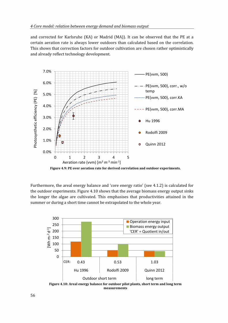
4 Core model: relation between energy demand and biomass output
56
and corrected for Karlsruhe (KA) or Madrid (MA)). It can be observed that the PE at a certain aeration rate is always lower outdoors than calculated based on the correlation. This shows that correction factors for outdoor cultivation are chosen rather optimistically and already reflect technology development.
Figure 4.9: PE over aeration rate for derived correlation and outdoor experiments.
Furthermore, the areal energy balance and ‘core energy ratio’ (see 4.1.2) is calculated for the outdoor experiments. Figure 4.10 shows that the average biomass energy output sinks the longer the algae are cultivated. This emphasises that productivities attained in the summer or during a short time cannot be extrapolated to the whole year.
Figure 4.10: Areal energy balance for outdoor pilot plants, short term and long term
measurements
0.0%
1.0%
2.0%
3.0%
4.0%
5.0%
6.0%
7.0%
0 1 2 3 4 5
Phot
osyn
thet
ic e
ffici
ency
(PE)
[%
]
Aeration rate (vvm) [m3 m-3 min-1]
PE(vvm, 500)
PE(vvm, 500), corr., w/otempPE(vvm, 500), corr.KA
PE(vvm, 500), corr.MA
Hu 1996
Rodolfi 2009
Quinn 2012
0.43 0.53 1.030
50100150200250300
Hu 1996 Rodolfi 2009 Quinn 2012
Outdoor short term long term
[Wh
m-2
d-1]
Operation energy inputBiomass energy output'CER' = Quotient in/out
CER:
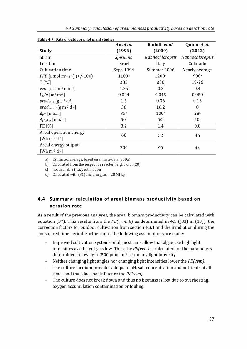
4.4 Summary: calculation of areal biomass productivity based on aeration rate
57
Table 4.7: Data of outdoor pilot plant studies
Study Hu et al. (1996)
Rodolfi et al. (2009)
Quinn et al. (2012)
Strain Spirulina Nannochloropsis Nannochloropsis Location Israel Italy Colorado Cultivation time Sept. 1994 Summer 2006 Yearly average PFD [µmol m-2 s-1] (+/-100) 1100a 1200a 900a T [°C] ≤35 ≤30 19-26 vvm [m3 m-3 min-1] 1.25 0.3 0.4 Vc/a [m3 m-2] 0.024 0.045 0.050 prodvol,d [g L-1 d-1] 1.5 0.36 0.16 prodarea,d [g m-2 d-1] 36 16.2 8 Δph [mbar] 35b 100b 28b Δpother [mbar] 50c 50c 50c PE [%] 3.2 1.4 0.8 Areal operation energy [Wh m-2 d-1]
60
52 46
Areal energy outputd [Wh m-2 d-1]
200
98 44
a) Estimated average, based on climate data (SoDa) b) Calculated from the respective reactor height with (20) c) not available (n.a.), estimation d) Calculated with (31) and energyDW = 20 MJ kg-1
4.4 Summary: calculation of areal biomass productivity based on aeration rate
As a result of the previous analyses, the areal biomass productivity can be calculated with equation (37). This results from the PE(vvm, I0) as determined in 4.1 ((33) in (13)), the correction factors for outdoor cultivation from section 4.3.1 and the irradiation during the considered time period. Furthermore, the following assumptions are made:
− Improved cultivation systems or algae strains allow that algae use high light intensities as efficiently as low. Thus, the PE(vvm) is calculated for the parameters determined at low light (500 µmol m-2 s-1) at any light intensity.
− Neither changing light angles nor changing light intensities lower the PE(vvm). − The culture medium provides adequate pH, salt concentration and nutrients at all
times and thus does not influence the PE(vvm). − The culture does not break down and thus no biomass is lost due to overheating,
oxygen accumulation contamination or fouling.
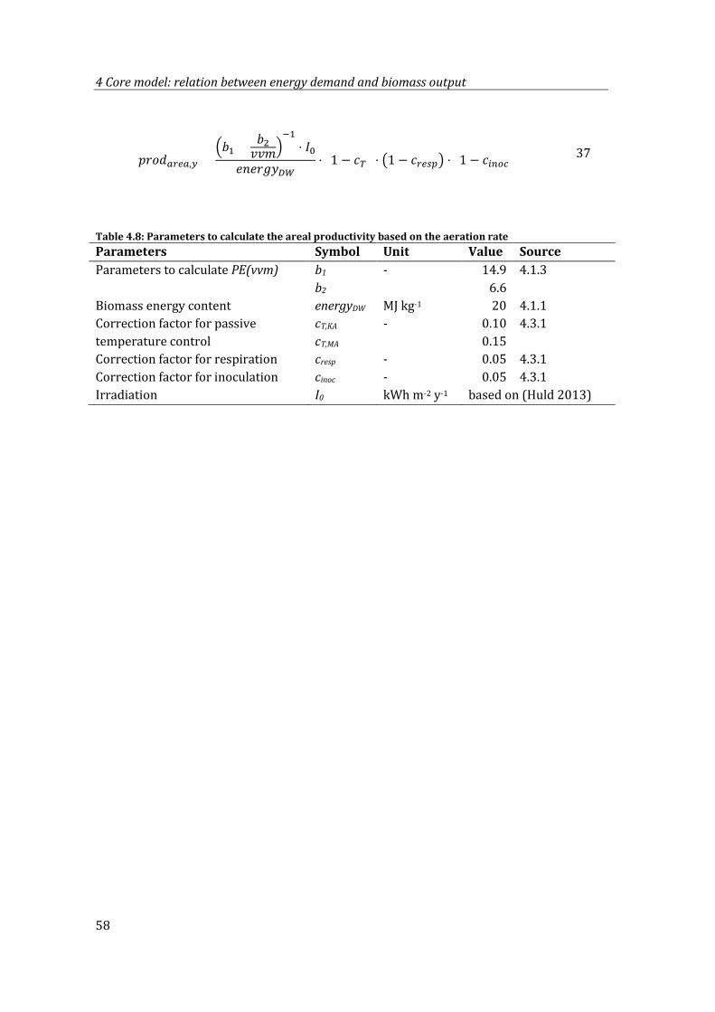
4 Core model: relation between energy demand and biomass output
58
𝑝𝑒𝑏𝑝𝑔𝑐𝑐𝑔,𝑦 =�𝑏1 + 𝑏2
𝑣𝑣𝑏�−1
⋅ 𝐼0
𝑒𝑛𝑒𝑒𝑒𝑒𝐷𝐷⋅ (1 − 𝑐𝑇) ⋅ �1 − 𝑐𝑐𝑐𝑔𝑝� ⋅ (1 − 𝑐𝑏𝑛𝑜𝑐) (37)
Table 4.8: Parameters to calculate the areal productivity based on the aeration rate Parameters Symbol Unit Value Source Parameters to calculate PE(vvm) b1
b2 - 14.9
6.6 4.1.3
Biomass energy content energyDW MJ kg-1 20 4.1.1 Correction factor for passive temperature control
cT,KA
cT,MA - 0.10
0.15 4.3.1
Correction factor for respiration cresp - 0.05 4.3.1 Correction factor for inoculation cinoc - 0.05 4.3.1 Irradiation I0 kWh m-2 y-1 based on (Huld 2013)
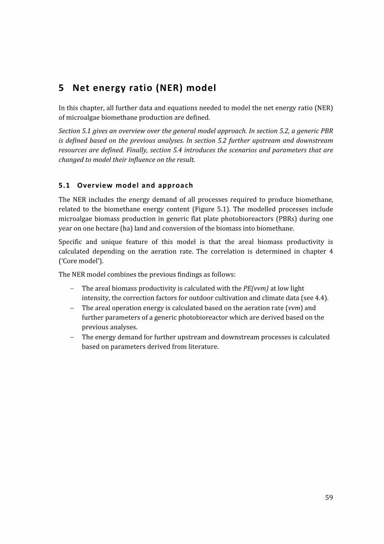
59
5 Net energy ratio (NER) model
In this chapter, all further data and equations needed to model the net energy ratio (NER) of microalgae biomethane production are defined.
Section 5.1 gives an overview over the general model approach. In section 5.2, a generic PBR is defined based on the previous analyses. In section 5.2 further upstream and downstream resources are defined. Finally, section 5.4 introduces the scenarios and parameters that are changed to model their influence on the result.
5.1 Overview model and approach
The NER includes the energy demand of all processes required to produce biomethane, related to the biomethane energy content (Figure 5.1). The modelled processes include microalgae biomass production in generic flat plate photobioreactors (PBRs) during one year on one hectare (ha) land and conversion of the biomass into biomethane.
Specific and unique feature of this model is that the areal biomass productivity is calculated depending on the aeration rate. The correlation is determined in chapter 4 (‘Core model’).
The NER model combines the previous findings as follows:
− The areal biomass productivity is calculated with the PE(vvm) at low light intensity, the correction factors for outdoor cultivation and climate data (see 4.4).
− The areal operation energy is calculated based on the aeration rate (vvm) and further parameters of a generic photobioreactor which are derived based on the previous analyses.
− The energy demand for further upstream and downstream processes is calculated based on parameters derived from literature.
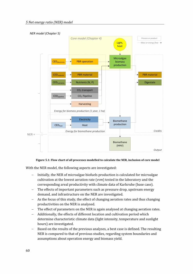
5 Net energy ratio (NER) model
60
PBR material
Nutrients (N, P)
CO2 Pipeline
CO2 transport
Harvesting
Electricity
Heat
Biomethane (HHV)
Process or product
Mass or energy flow
Credits
Energy for biomass production (1 year, 1 ha)
Energy for biomethane production
CEDelectricity
CEDmaterial
CEDnutrients
CEDpipeline
CEDheat
Digestate
PBR material
Core model (Chapter 4)Light, heat
NER model (Chapter 5)
PBR operation
Output
Biomethane production
Microalgae biomass
production
NER =
Figure 5.1: Flow chart of all processes modelled to calculate the NER, inclusion of core model
With the NER model, the following aspects are investigated:
− Initially, the NER of microalgae biofuels production is calculated for microalgae cultivation at the lowest aeration rate (vvm) tested in the laboratory and the corresponding areal productivity with climate data of Karlsruhe (base case).
− The effects of important parameters such as pressure drop, upstream energy demand, and infrastructure on the NER are investigated.
− As the focus of this study, the effect of changing aeration rates and thus changing productivities on the NER is analysed.
− The effect of parameters on the NER is again analysed at changing aeration rates. − Additionally, the effects of different location and cultivation period which
determine characteristic climate data (light intensity, temperature and sunlight hours) are investigated.
− Based on the results of the previous analyses, a best case is defined. The resulting NER is compared to that of previous studies, regarding system boundaries and assumptions about operation energy and biomass yield.
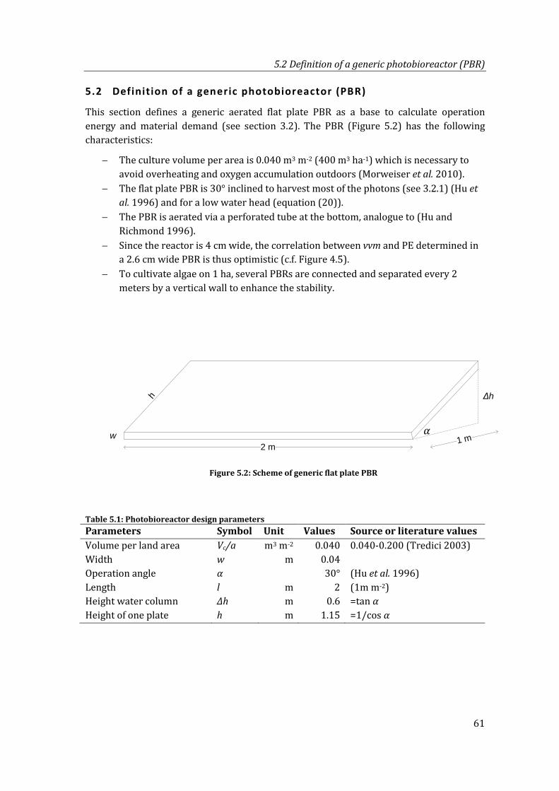
5.2 Definition of a generic photobioreactor (PBR)
61
5.2 Definition of a generic photobioreactor (PBR)
This section defines a generic aerated flat plate PBR as a base to calculate operation energy and material demand (see section 3.2). The PBR (Figure 5.2) has the following characteristics:
− The culture volume per area is 0.040 m3 m-2 (400 m3 ha-1) which is necessary to avoid overheating and oxygen accumulation outdoors (Morweiser et al. 2010).
− The flat plate PBR is 30° inclined to harvest most of the photons (see 3.2.1) (Hu et al. 1996) and for a low water head (equation (20)).
− The PBR is aerated via a perforated tube at the bottom, analogue to (Hu and Richmond 1996).
− Since the reactor is 4 cm wide, the correlation between vvm and PE determined in a 2.6 cm wide PBR is thus optimistic (c.f. Figure 4.5).
− To cultivate algae on 1 ha, several PBRs are connected and separated every 2 meters by a vertical wall to enhance the stability.
𝛼1 m
2 mw
Δhh
Figure 5.2: Scheme of generic flat plate PBR
Table 5.1: Photobioreactor design parameters Parameters Symbol Unit Values Source or literature values Volume per land area Vc/a m3 m-2 0.040 0.040-0.200 (Tredici 2003) Width w m 0.04 Operation angle 𝛼 30° (Hu et al. 1996) Length l m 2 (1m m-2) Height water column Δh m 0.6 =tan 𝛼 Height of one plate h m 1.15 =1/cos 𝛼
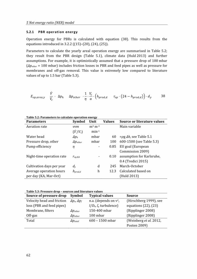
5 Net energy ratio (NER) model
62
5.2.1 PBR operation energy
Operation energy for PBRs is calculated with equation (38). This results from the equations introduced in 3.2.2 ((15)–(20), (24), (25)).
Parameters to calculate the yearly areal operation energy are summarised in Table 5.2; they result from the PBR design (Table 5.1), climate data (Huld 2013) and further assumptions. For example, it is optimistically assumed that a pressure drop of 100 mbar (Δpother = 100 mbar) includes friction losses in PBR and feed pipes as well as pressure for membranes and off-gas removal. This value is extremely low compared to literature values of up to 1.5 bar (Table 5.3).
𝑁𝑜𝑝,𝑔𝑐𝑐𝑔,𝑦 =�̇�𝑉𝑐
⋅ (∆𝑝ℎ + ∆𝑝𝑜𝑡ℎ𝑐𝑐) ⋅1𝜂
⋅𝑉𝑐
𝑏⋅ �ℎ𝑝𝑐𝑜𝑐,𝑐 + 𝑒𝑜𝑝 ⋅ �24 − ℎ𝑝𝑐𝑜𝑐,𝑐�� ⋅ 𝑝𝑦 (38)
Table 5.2: Parameters to calculate operation energy Parameters Symbol Unit Values Source or literature values Aeration rate vvm
(�̇�/Vc) m3 m-3
min-1 Main variable
Water head Δph mbar 60 =ρg Δh, see Table 5.1 Pressure drop, other Δpother mbar 100 600-1500 (see Table 5.3) Pump efficiency η - 0.85 EU goal (European
Commission 2009) Night-time operation rate rop,KA - 0.10 assumption for Karlsruhe,
0.4 (Tredici 2015) Cultivation days per year dy d 245 March-October Average operation hours per day (KA, Mar-Oct)
hprod,d h 12.3 Calculated based on (Huld 2013)
Table 5.3: Pressure drop – sources and literature values Source of pressure drop Symbol Typical values Source Velocity head and friction loss (PBR and feed pipes)
Δpv, Δpf n.a. (depends on v2, l/Dh, ζ, turbulence)
(Hirschberg 1999), see equations (22), (23)
Membrane, filters Δpother 150-400 mbar (Ripplinger 2008) Off-gas Δpother 100 mbar (Ripplinger 2008) Total Δptotal 600 – 1500 mbar (Weinberg et al. 2012,
Posten 2009)
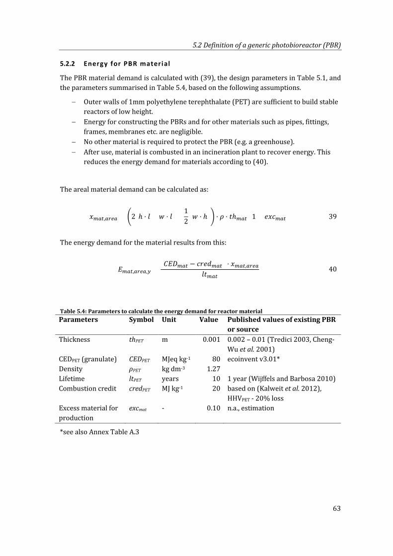
5.2 Definition of a generic photobioreactor (PBR)
63
5.2.2 Energy for PBR material
The PBR material demand is calculated with (39), the design parameters in Table 5.1, and the parameters summarised in Table 5.4, based on the following assumptions.
− Outer walls of 1mm polyethylene terephthalate (PET) are sufficient to build stable reactors of low height.
− Energy for constructing the PBRs and for other materials such as pipes, fittings, frames, membranes etc. are negligible.
− No other material is required to protect the PBR (e.g. a greenhouse). − After use, material is combusted in an incineration plant to recover energy. This
reduces the energy demand for materials according to (40).
The areal material demand can be calculated as:
𝑥𝑚𝑔𝑡,𝑔𝑐𝑐𝑔 = �2(ℎ ⋅ 𝑙 + 𝑤 ⋅ 𝑙) +12
(𝑤 ⋅ ℎ)� ⋅ 𝜌 ⋅ 𝑡ℎ𝑚𝑔𝑡 (1 + 𝑒𝑥𝑐𝑚𝑔𝑡) (39)
The energy demand for the material results from this:
𝑁𝑚𝑔𝑡,𝑔𝑐𝑐𝑔,𝑦 =(𝐶𝑁𝐶𝑚𝑔𝑡 − 𝑐𝑒𝑒𝑝𝑚𝑔𝑡) ⋅ 𝑥𝑚𝑔𝑡,𝑔𝑐𝑐𝑔
𝑙𝑡𝑚𝑔𝑡 (40)
Table 5.4: Parameters to calculate the energy demand for reactor material Parameters Symbol Unit Value Published values of existing PBR
or source Thickness thPET m 0.001 0.002 – 0.01 (Tredici 2003, Cheng-
Wu et al. 2001) CEDPET (granulate) CEDPET MJeq kg-1 80 ecoinvent v3.01* Density ρPET kg dm-3 1.27 Lifetime ltPET years 10 1 year (Wijffels and Barbosa 2010) Combustion credit credPET MJ kg-1 20 based on (Kalweit et al. 2012),
HHVPET - 20% loss Excess material for production
excmat - 0.10 n.a., estimation
*see also Annex Table A.3
5 Net energy ratio (NER) model
64
5.3 Calculation of other energy demand
This section defines the energy demand for upstream and downstream resources. The energy demand for each resource results from the required amount (xn), multiplied with the respective cumulative energy demand (CEDn) and credits where appropriate (see 2.1.2).
The nutrient and CO2 demand is calculated directly proportional to the produced biomass, so is the energy to ferment the biomass. Electricity for harvesting is related to the culture volume (see 3.2.2). Infrastructure includes, apart from the PBR, only pipelines to supply CO2.
5.3.1 Upstream: supply of resources
CO2 and nutrients
The resources to supply CO2 are calculated with (41) and (42), assuming that:
− Microalgae require 1.8 kg CO2 per kg dry weight (Kliphuis et al. 2010) and take up 90% of the supplied CO2.
− An industrial power plant provides CO2; no energy is accounted for CO2 separation. − CO2 is compressed to 22 bar for a low pressure transport over 15 km in pipelines
(Skarka 2015).
𝑥𝐶𝐶2,𝑔𝑐𝑐𝑔,𝑦 = 𝑝𝑒𝑏𝑝𝑔𝑐𝑐𝑔,𝑦 ⋅𝑏𝐶𝐶2
𝑏𝑏𝑏⋅ 𝑁𝑡𝑐,𝐶𝐶2 (41)
𝑥𝑝𝑏𝑝𝑐𝑓𝑏𝑛𝑐,𝑦 =𝑙𝑒𝑛𝑒𝑡ℎ𝑝𝑏𝑝
𝑙𝑡𝑝𝑏𝑝 (42)
The nutrient demand is calculated with (43) under the assumptions that:
− Microalgae biomass consists of 6.6% and 1.3% (w/w) nitrogen and (N) phosphorous (P) respectively (Grobbelaar 2003). The culture medium contains 20% excess nutrients (Richmond and Cheng-Wu 2001) to ensure that microalgae can take them up sufficiently.
− 80% of N and 99% of P in the digested biomass could be used again as fertiliser (Rösch et al. 2012) and are credited as such. Excess nutrients are not taken up and thus not credited.
𝑥(𝑁,𝑃),𝑔𝑐𝑐𝑔,𝑦 = 𝑝𝑒𝑏𝑝𝑔𝑐𝑐𝑔,𝑦 ⋅ 𝑏𝑁,𝑃�𝑒𝑥𝑐𝑁,𝑃 − 𝑐𝑒𝑒𝑝𝑁,𝑃� (43)
Furthermore, the following simplifications are made:
− Energy demand to supply other (micro-) nutrients is negligible.
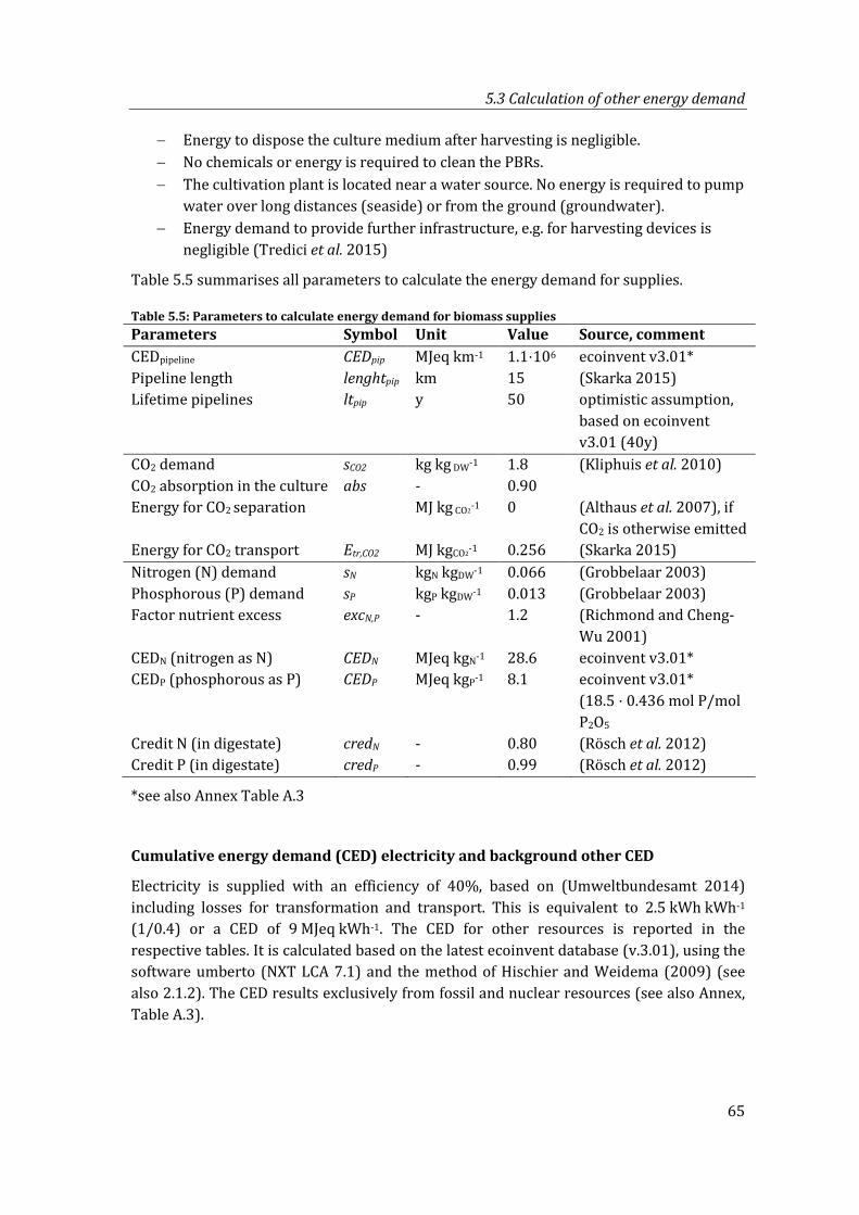
5.3 Calculation of other energy demand
65
− Energy to dispose the culture medium after harvesting is negligible. − No chemicals or energy is required to clean the PBRs. − The cultivation plant is located near a water source. No energy is required to pump
water over long distances (seaside) or from the ground (groundwater). − Energy demand to provide further infrastructure, e.g. for harvesting devices is
negligible (Tredici et al. 2015)
Table 5.5 summarises all parameters to calculate the energy demand for supplies.
Table 5.5: Parameters to calculate energy demand for biomass supplies Parameters Symbol Unit Value Source, comment CEDpipeline CEDpip MJeq km-1 1.1⋅106 ecoinvent v3.01* Pipeline length lenghtpip km 15 (Skarka 2015) Lifetime pipelines ltpip y 50 optimistic assumption,
based on ecoinvent v3.01 (40y)
CO2 demand sCO2 kg kg DW-1 1.8 (Kliphuis et al. 2010) CO2 absorption in the culture abs - 0.90 Energy for CO2 separation MJ kg CO2-1 0 (Althaus et al. 2007), if
CO2 is otherwise emitted Energy for CO2 transport Etr,CO2 MJ kgCO2-1 0.256 (Skarka 2015) Nitrogen (N) demand sN kgN kgDW-1 0.066 (Grobbelaar 2003) Phosphorous (P) demand sP kgP kgDW-1 0.013 (Grobbelaar 2003) Factor nutrient excess excN,P - 1.2 (Richmond and Cheng-
Wu 2001) CEDN (nitrogen as N) CEDN MJeq kgN-1 28.6 ecoinvent v3.01* CEDP (phosphorous as P) CEDP MJeq kgP-1 8.1 ecoinvent v3.01*
(18.5 ⋅ 0.436 mol P/mol P2O5)
Credit N (in digestate) credN - 0.80 (Rösch et al. 2012) Credit P (in digestate) credP - 0.99 (Rösch et al. 2012)
*see also Annex Table A.3
Cumulative energy demand (CED) electricity and background other CED
Electricity is supplied with an efficiency of 40%, based on (Umweltbundesamt 2014) including losses for transformation and transport. This is equivalent to 2.5 kWh kWh-1 (1/0.4) or a CED of 9 MJeq kWh-1. The CED for other resources is reported in the respective tables. It is calculated based on the latest ecoinvent database (v.3.01), using the software umberto (NXT LCA 7.1) and the method of Hischier and Weidema (2009) (see also 2.1.2). The CED results exclusively from fossil and nuclear resources (see also Annex, Table A.3).
5 Net energy ratio (NER) model
66
5.3.2 Downstream: harvesting and biomethane production
The energy for harvesting and culture transport is related to the culture volume. The energy for fermentation and biogas upgrading is proportional to the amount of produced biomethane (and thus also to the microalgae biomass).
Harvesting & culture transport
The energy demand for harvesting and culture transport is calculated with equations (26)- (28) and the following data and simplifications:
− Microalgae are harvested with a separator with 1.5 kW power demand and a capacity of 1.2 m³ h-1, resulting in a volumetric harvesting energy of 1.25 kWh m-3. Posten et al. (2012) expect this energy demand for harvesting representing technical progress.
− The whole culture medium is exchanged every 10 days (dex = 10) and the pump for culture exchange requires 0.13 kWh m-3 (Norsker et al. 2011). The batch length does not influence the biomass productivity.
− No additional pump energy, devices, space or chemicals are required to pre-concentrate the biomass (e.g. by settling the algae in ponds).
Biomethane production
Energy for biomass fermentation is calculated with the data summarised in Table 5.6 and the following simplifications:
− Harvesting concentrates the biomass up to a total solids (TS) content of 2-10% required for wet fermentation.
− The biogas is upgraded to methane and fed into the natural gas network. The energy to operate the biogas plant is thus supplied externally (Jungbluth et al. 2007). (Different scenarios of internal and external biogas energy use are analysed in Weinberg et al. (2012)).
− The biogas plant has a long lifetime and is only partially used for algae biomass. Thus, the CED to construct the biogas plant is negligible compared to the operation energy.
− The methane yield is directly proportional to the microalgal biomass (44).
𝑋𝑚𝑐𝑡ℎ,𝑔𝑐𝑐𝑔,𝑦 = 𝑝𝑒𝑏𝑝𝑔𝑐𝑐𝑔,𝑦 ⋅ 𝑏𝑚𝑐𝑡ℎ (44)
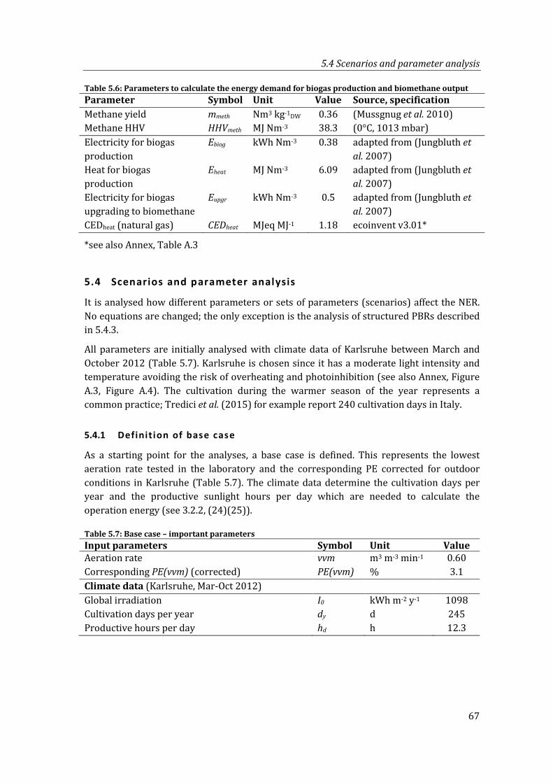
5.4 Scenarios and parameter analysis
67
Table 5.6: Parameters to calculate the energy demand for biogas production and biomethane output Parameter Symbol Unit Value Source, specification Methane yield mmeth Nm3 kg-1DW 0.36 (Mussgnug et al. 2010) Methane HHV HHVmeth MJ Nm-3 38.3 (0°C, 1013 mbar) Electricity for biogas production
Ebiog kWh Nm-3 0.38 adapted from (Jungbluth et al. 2007)
Heat for biogas production
Eheat MJ Nm-3 6.09 adapted from (Jungbluth et al. 2007)
Electricity for biogas upgrading to biomethane
Eupgr kWh Nm-3 0.5 adapted from (Jungbluth et al. 2007)
CEDheat (natural gas) CEDheat MJeq MJ-1 1.18 ecoinvent v3.01*
*see also Annex, Table A.3
5.4 Scenarios and parameter analysis
It is analysed how different parameters or sets of parameters (scenarios) affect the NER. No equations are changed; the only exception is the analysis of structured PBRs described in 5.4.3.
All parameters are initially analysed with climate data of Karlsruhe between March and October 2012 (Table 5.7). Karlsruhe is chosen since it has a moderate light intensity and temperature avoiding the risk of overheating and photoinhibition (see also Annex, Figure A.3, Figure A.4). The cultivation during the warmer season of the year represents a common practice; Tredici et al. (2015) for example report 240 cultivation days in Italy.
5.4.1 Definition of base case
As a starting point for the analyses, a base case is defined. This represents the lowest aeration rate tested in the laboratory and the corresponding PE corrected for outdoor conditions in Karlsruhe (Table 5.7). The climate data determine the cultivation days per year and the productive sunlight hours per day which are needed to calculate the operation energy (see 3.2.2, (24)(25)).
Table 5.7: Base case – important parameters Input parameters Symbol Unit Value Aeration rate vvm m3 m-3 min-1 0.60 Corresponding PE(vvm) (corrected) PE(vvm) % 3.1 Climate data (Karlsruhe, Mar-Oct 2012) Global irradiation I0 kWh m-2 y-1 1098 Cultivation days per year dy d 245 Productive hours per day hd h 12.3
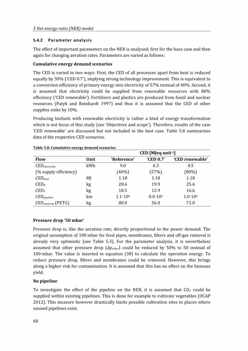
5 Net energy ratio (NER) model
68
5.4.2 Parameter analysis
The effect of important parameters on the NER is analysed; first for the base case and then again for changing aeration rates. Parameters are varied as follows:
Cumulative energy demand scenarios
The CED is varied in two ways: First, the CED of all processes apart from heat is reduced equally by 30% (‘CED 0.7’), implying strong technology improvement. This is equivalent to a conversion efficiency of primary energy into electricity of 57% instead of 40%. Second, it is assumed that electricity could be supplied from renewable resources with 80% efficiency (‘CED renewable’). Fertilisers and plastics are produced from fossil and nuclear resources (Patyk and Reinhardt 1997) and thus it is assumed that the CED of other supplies sinks by 10%.
Producing biofuels with renewable electricity is rather a kind of energy transformation which is not focus of this study (see ‘Objectives and scope’). Therefore, results of the case ‘CED renewable’ are discussed but not included in the best case. Table 5.8 summarises data of the respective CED scenarios.
Table 5.8: Cumulative energy demand scenarios CED [MJeq unit-1] Flow Unit ‘Reference’ ‘CED 0.7’ ‘CED renewable’ CEDelectricity (% supply efficiency)
kWh
9.0 (40%)
6.3 (57%)
4.5 (80%)
CEDheat MJ 1.18 1.18 1.18 CEDN kg 28.6 19.9 25.6 CEDP kg 18.5 12.9 16.6 CEDpipeline km 1.1⋅106 8.0⋅105 1.0⋅106 CEDmaterial (PETG) kg 80.0 56.0 72.0
Pressure drop ’50 mbar’
Pressure drop is, like the aeration rate, directly proportional to the power demand. The original assumption of 100 mbar for feed pipes, membranes, filters and off-gas removal is already very optimistic (see Table 5.3). For the parameter analysis, it is nevertheless assumed that other pressure drop (Δpother) could be reduced by 50% to 50 instead of 100 mbar. The value is inserted in equation (38) to calculate the operation energy. To reduce pressure drop, filters and membranes could be removed. However, this brings along a higher risk for contamination. It is assumed that this has no effect on the biomass yield.
No pipeline
To investigate the effect of the pipeline on the NER, it is assumed that CO2 could be supplied within existing pipelines. This is done for example to cultivate vegetables (OCAP 2012). This measure however drastically limits possible cultivation sites to places where unused pipelines exist.
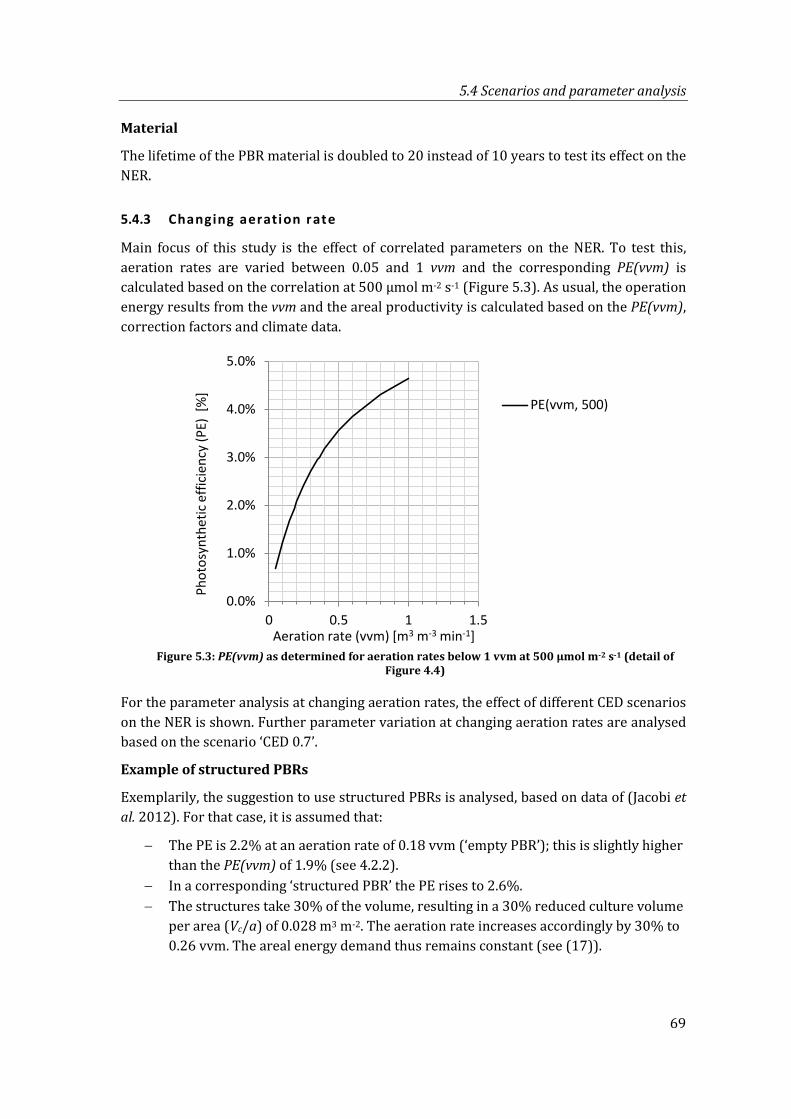
5.4 Scenarios and parameter analysis
69
Material
The lifetime of the PBR material is doubled to 20 instead of 10 years to test its effect on the NER.
5.4.3 Changing aeration rate
Main focus of this study is the effect of correlated parameters on the NER. To test this, aeration rates are varied between 0.05 and 1 vvm and the corresponding PE(vvm) is calculated based on the correlation at 500 µmol m-2 s-1 (Figure 5.3). As usual, the operation energy results from the vvm and the areal productivity is calculated based on the PE(vvm), correction factors and climate data.
Figure 5.3: PE(vvm) as determined for aeration rates below 1 vvm at 500 µmol m-2 s-1 (detail of
Figure 4.4)
For the parameter analysis at changing aeration rates, the effect of different CED scenarios on the NER is shown. Further parameter variation at changing aeration rates are analysed based on the scenario ‘CED 0.7’.
Example of structured PBRs
Exemplarily, the suggestion to use structured PBRs is analysed, based on data of (Jacobi et al. 2012). For that case, it is assumed that:
− The PE is 2.2% at an aeration rate of 0.18 vvm (‘empty PBR’); this is slightly higher than the PE(vvm) of 1.9% (see 4.2.2).
− In a corresponding ‘structured PBR’ the PE rises to 2.6%. − The structures take 30% of the volume, resulting in a 30% reduced culture volume
per area (Vc/a) of 0.028 m3 m-2. The aeration rate increases accordingly by 30% to 0.26 vvm. The areal energy demand thus remains constant (see (17)).
0.0%
1.0%
2.0%
3.0%
4.0%
5.0%
0 0.5 1 1.5
Phot
osyn
thet
ic e
ffici
ency
(PE)
[%
]
Aeration rate (vvm) [m3 m-3 min-1]
PE(vvm, 500)
5 Net energy ratio (NER) model
70
5.4.4 Location and cultivation period
Location and cultivation period are varied. Those determine light intensity, temperature and sunlight hours per day.
First, the effect of cultivating algae at a different location is determined. The areal biomass productivity at a certain aeration rate is calculated with climate data of Madrid (MA) instead of Karlsruhe (KA). To account for higher temperature and light intensity in Madrid (see also Annex, Figure A.2), a higher temperature correction factor and night-time operation rate is assumed (Table 5.9). The cultivation period remains constant (March-October, blue row in Table 5.10).
Second, it is analysed how the cultivation period affects the NER. For this, the cultivation period is reduced step-wise by two months, beginning with a year-round cultivation (see Table 5.10). Results are shown for both locations at a constant aeration rate. Exemplarily, it is shown for Karlsruhe how cultivation period and aeration rate interact.
Table 5.9: Temperature correction factors and night-time operation rate for Karlsruhe and Madrid Parameter Karlsruhe (KA) Madrid (MA) Literature data cT 0.10 0.15 0.40-0.60 (Hu et al. 1996) r 0.10 0.20 0.42 Italy (Tredici et al. 2015)
Table 5.10: Location and cultivation period – input parameters, based on (Huld 2013) Cultivation period (2012)
dy Average irradiation hours
per day hd
Solar irradiation [kWh m-2 y-1]
Average light intensity (day)
[W m-2] KA MA KA MA KA MA January-December 366* 10.4 10.7 1220 1790 320 460 February-November 304* 11.4 11.4 1180 1660 340 480 March-October 245 12.3 12.1 1100 1500 360 510 April-September 183 12.8 12.3 920 1230 390 550 May-August 123 13.3 12.5 680 920 420 600 June-July 61 13.8 12.7 340 480 400 630
*2012 is a leap year
71
6 Results and discussion
The NER of biomethane production from microalgae cultivated in generic aerated photobioreactors is calculated based on the correlation between aeration rate and PE determined in chapter 4 and further data and equations summarised in chapter 5. In this chapter, important results are shown and discussed.
Section 6.1 shows the NER of the base case. The influence of the different parameters on the base case is examined in section 6.2. In sections 6.3 and 6.4 as the central points of this investigation, it is demonstrated how the NER changes with the aeration rate – and how consequently parameter variations affect the NER at changing aeration rates. In section 6.5, the effects of a different location and different cultivation periods on the NER are shown – also in combination with changing aeration rate. In section 6.6, the main findings are summarised and a best case scenario is defined. This best case is in section 6.7 compared to the best cases of previous studies concerning (i) system boundaries and (ii) assumptions about key parameters. The potential technology improvement is also discussed. Finally, limitations of this approach and suggestions for further work are presented in section 6.8.
6.1 Base case
The base case represents the NER of biomethane production from microalgae cultivated in Karlsruhe during March-October in a photobioreactor aerated at 0.6 vvm. Table 6.1 summarises characteristic operation and productivity parameters of the base case.
Table 6.1: Operation and productivity parameters (base case) Characteristic parameters Symbol Unit Value Operation power, volumetric Pvol W m-3 188 Operation power, areal Parea W m-2 7.5 Operation energy, areal (24h) Eop,area,d kWh m-2 d-1 0.10 Yearly biomass yield Yha,y t ha-1 y-1 62 Average areal productivity (per day) prodarea,d g m-2 d-1 25 Average volumetric productivity (per day) prodvol,d g L-1 d-1 0.63
In total, all considered processes and substances require about 4 times more energy than the biomethane contains; the NER is 4.0 (Figure 6.1).
Operation energy dominates the total energy demand or input with around 65%. Additional 25% of the total energy demand is required for biomass production and harvesting; only about 10% are required to convert biomass into methane. Apart from operation energy, pipeline and material demand have a large share on the energy input. Nutrients hardly contribute to the high NER since it is assumed that the major part of nutrients remains in the digestate and could be recycled as fertiliser (Table 6.2).
6 Results and discussion
72
Figure 6.1: Energy input (cumulative energy demand) and output (HHV biomethane) per hectare
and year (base case)
Table 6.2: Resource demand per hectare and year, resulting energy demand and NER (base case)
Value Unit
ha-1 y-1 Input [GJeq]
Credits [GJeq]
Output [GJeq]
MJeq MJ-1 methane
Operation 227 MWh 2042 2.39 Operation nighttime 22 MWh 194 0.23 Culture transport 2.6 MWh 23 0.03 Harvesting 12.5 MWh 113 0.13 PBR Material 3.4 t 270 67 0.24 Nitrogen 4.9 t 139 92 0.05 Phosphorous 1.0 t 8 7 0.00 CO2 transport 8.8 MWh 79 0.09 CO2 pipeline 0.3 km 341 0.40 Biogas: heat 136 GJ 161 0.19 Biogas: energy 8.4 MWh 76 0.09 Biogas: upgrading 11.1 MWh 100 0.12 OUTPUT Biomethane 856 Totals 3546 166 4.0
0.0E+00
5.0E+05
1.0E+06
1.5E+06
2.0E+06
2.5E+06
3.0E+06
3.5E+06
4.0E+06
Input [MJ-eq] Output [MJ]
[MJ h
a-1y-1
]OUTPUT Biomethane
Biogas: upgrading
Biogas: energy
Biogas: heat
CO pipeline
CO transport
Phosphorous (-credit)
Nitrogen (-credit)
PBR Material (-credit)
Harvesting
Culture transport
Operation nighttime
Operation
2
2
6.2 Base case – parameter analysis
73
The biomass yield of 62 tons per ha and year is within the range of 60–70 t ha-1 y-1
expected to be “realistic” for PBRs (Chiaramonti et al. 2013). The operation power of less than 200 W m-3 is a goal of current PBR development (Posten 2009).
Regarding the areal energy balance, the areal operation energy (227+22 MWh ha-1 y-1, see Table 6.2) is still lower than the energy contained in the biomass, but already higher than the biomethane energy produced from that (Figure 6.2). Reasons are additional night-time operation and respiration losses but also that only a share of the biomass energy content can be turned into biomethane energy.
The biomethane yield together with its heating value results in 14 MJHHV kg-1DW (0.36 Nm3 kg-1DW ⋅ 38.3 MJ Nm-3, see Table 5.6). Compared to 20 MJHHV kg-1DW in the biomass (see Table 4.8), this corresponds to an ‘energy yield’ of 70%. This assumption is higher than for example that of Weinberg et al. (2012) who calculate with a biomethane yield of 11 MJHHV kg-1DW (10.4 MJLHV kg-1DW ).
Figure 6.2: Areal operation energy, energy content in biomass (intermediate) and biomethane
energy (base case)
6.2 Base case – parameter analysis
The impact of parameter changes on the base case is analysed.
6.2.1 Cumulative energy demand
The CED is linearly related to all input flows. Therefore, assumptions about the CED strongly influence the NER. Nevertheless, all CED scenarios result in a NER > 1. The CED for operation exceeds 1 but also without any operation energy, between 1.1-1.6 MJeq per MJ biomethane are needed for other supplies and processes (Table 6.3).
Note that the scenario ‘CED 0.7’ equally reduces all energy demand while the scenario ‘CED renewable’ reduces mainly energy demand for electricity and thus also changes the proportion of operation energy to other energy demand (Figure 6.3).
0
50
100
150
200
250
300
350
400
Areal energydemand operation
(day+night, no CED)
Areal energy outputin biomass
(intermediate)
Areal energy outputbiomethane
[MW
h ha
-1y-1
]
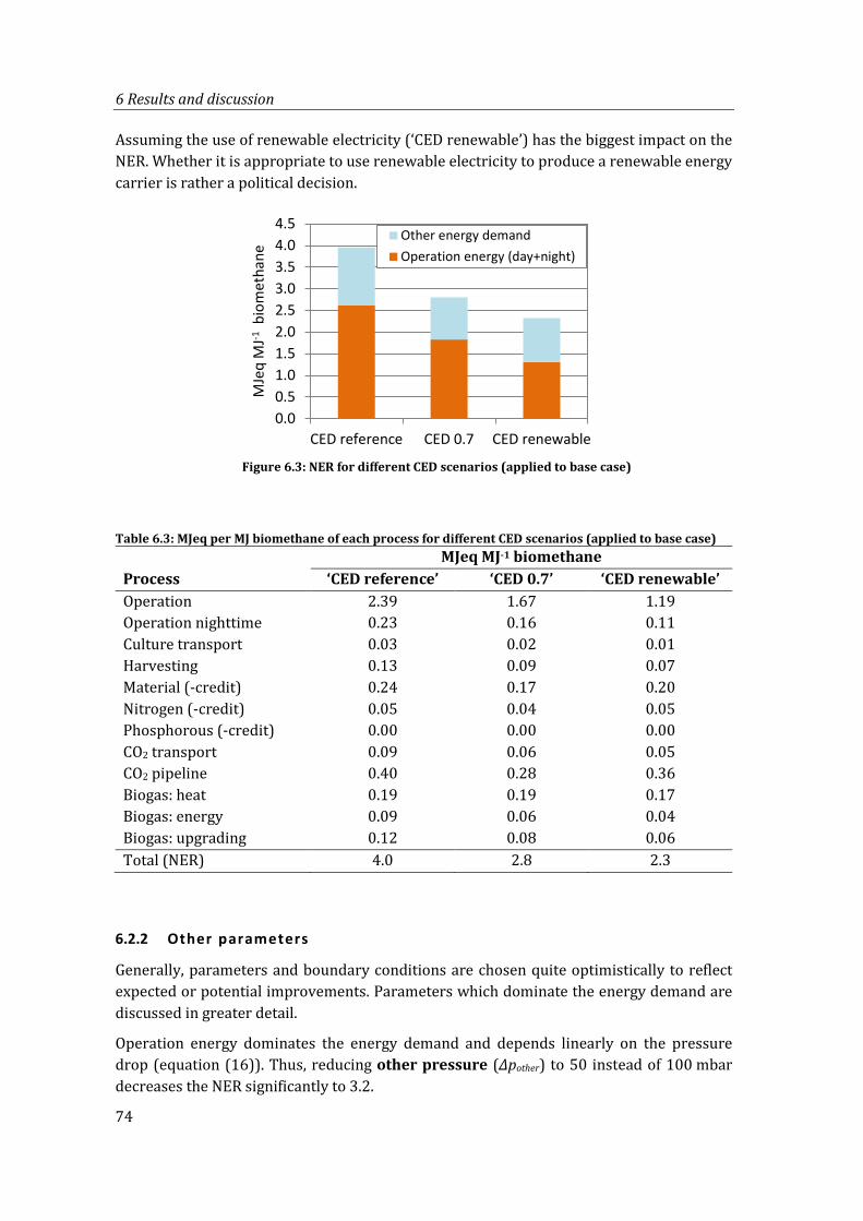
6 Results and discussion
74
Assuming the use of renewable electricity (‘CED renewable’) has the biggest impact on the NER. Whether it is appropriate to use renewable electricity to produce a renewable energy carrier is rather a political decision.
Figure 6.3: NER for different CED scenarios (applied to base case)
Table 6.3: MJeq per MJ biomethane of each process for different CED scenarios (applied to base case) MJeq MJ-1 biomethane Process ‘CED reference’ ‘CED 0.7’ ‘CED renewable’ Operation 2.39 1.67 1.19 Operation nighttime 0.23 0.16 0.11 Culture transport 0.03 0.02 0.01 Harvesting 0.13 0.09 0.07 Material (-credit) 0.24 0.17 0.20 Nitrogen (-credit) 0.05 0.04 0.05 Phosphorous (-credit) 0.00 0.00 0.00 CO2 transport 0.09 0.06 0.05 CO2 pipeline 0.40 0.28 0.36 Biogas: heat 0.19 0.19 0.17 Biogas: energy 0.09 0.06 0.04 Biogas: upgrading 0.12 0.08 0.06 Total (NER) 4.0 2.8 2.3
6.2.2 Other parameters
Generally, parameters and boundary conditions are chosen quite optimistically to reflect expected or potential improvements. Parameters which dominate the energy demand are discussed in greater detail.
Operation energy dominates the energy demand and depends linearly on the pressure drop (equation (16)). Thus, reducing other pressure (Δpother) to 50 instead of 100 mbar decreases the NER significantly to 3.2.
0.00.51.01.52.02.53.03.54.04.5
CED reference CED 0.7 CED renewable
MJe
q M
J-1bi
omet
hane
Other energy demandOperation energy (day+night)
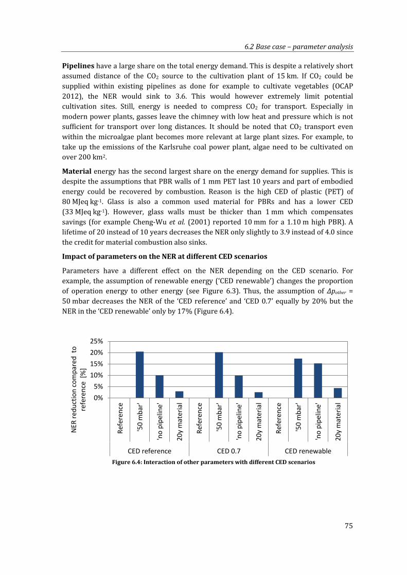
6.2 Base case – parameter analysis
75
Pipelines have a large share on the total energy demand. This is despite a relatively short assumed distance of the CO2 source to the cultivation plant of 15 km. If CO2 could be supplied within existing pipelines as done for example to cultivate vegetables (OCAP 2012), the NER would sink to 3.6. This would however extremely limit potential cultivation sites. Still, energy is needed to compress CO2 for transport. Especially in modern power plants, gasses leave the chimney with low heat and pressure which is not sufficient for transport over long distances. It should be noted that CO2 transport even within the microalgae plant becomes more relevant at large plant sizes. For example, to take up the emissions of the Karlsruhe coal power plant, algae need to be cultivated on over 200 km2.
Material energy has the second largest share on the energy demand for supplies. This is despite the assumptions that PBR walls of 1 mm PET last 10 years and part of embodied energy could be recovered by combustion. Reason is the high CED of plastic (PET) of 80 MJeq kg-1. Glass is also a common used material for PBRs and has a lower CED (33 MJeq kg-1). However, glass walls must be thicker than 1 mm which compensates savings (for example Cheng-Wu et al. (2001) reported 10 mm for a 1.10 m high PBR). A lifetime of 20 instead of 10 years decreases the NER only slightly to 3.9 instead of 4.0 since the credit for material combustion also sinks.
Impact of parameters on the NER at different CED scenarios
Parameters have a different effect on the NER depending on the CED scenario. For example, the assumption of renewable energy (‘CED renewable’) changes the proportion of operation energy to other energy (see Figure 6.3). Thus, the assumption of Δpother = 50 mbar decreases the NER of the ‘CED reference’ and ‘CED 0.7’ equally by 20% but the NER in the ‘CED renewable’ only by 17% (Figure 6.4).
Figure 6.4: Interaction of other parameters with different CED scenarios
0%5%
10%15%20%25%
Refe
renc
e
'50
mba
r'
'no
pipe
line'
20y
mat
eria
l
Refe
renc
e
'50
mba
r'
'no
pipe
line'
20y
mat
eria
l
Refe
renc
e
'50
mba
r'
'no
pipe
line'
20y
mat
eria
l
CED reference CED 0.7 CED renewable
NER
redu
ctio
n co
mpa
red
to
refe
renc
e [%
]
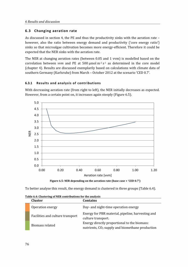
6 Results and discussion
76
6.3 Changing aeration rate
As discussed in section 4, the PE and thus the productivity sinks with the aeration rate – however, also the ratio between energy demand and productivity (‘core energy ratio’) sinks so that microalgae cultivation becomes more energy-efficient. Therefore it could be expected that the NER sinks with the aeration rate.
The NER at changing aeration rates (between 0.05 and 1 vvm) is modelled based on the correlation between vvm and PE at 500 µmol m-2 s-1 as determined in the core model (chapter 4). Results are discussed exemplarily based on calculations with climate data of southern Germany (Karlsruhe) from March – October 2012 at the scenario ‘CED 0.7’.
6.3.1 Results and analysis of contributions
With decreasing aeration rate (from right to left), the NER initially decreases as expected. However, from a certain point on, it increases again steeply (Figure 6.5).
Figure 6.5: NER depending on the aeration rate (base case + ‘CED 0.7’)
To better analyse this result, the energy demand is clustered in three groups (Table 6.4).
Table 6.4: Clustering of NER contributions for the analysis Cluster Contains
Operation energy Day- and night-time operation energy
Facilities and culture transport
Energy for PBR material, pipeline, harvesting and culture transport.
Biomass related
Energy directly proportional to the biomass: nutrients, CO2 supply and biomethane production
0.0
0.5
1.0
1.5
2.0
2.5
3.0
3.5
4.0
4.5
5.0
0.00 0.20 0.40 0.60 0.80 1.00 1.20
NER
Aeration rate [vvm]
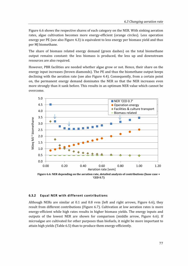
6.3 Changing aeration rate
77
Figure 6.6 shows the respective shares of each category on the NER. With sinking aeration rates, algae cultivation becomes more energy-efficient (orange circles). Less operation energy per PE (see also Figure 4.3) is equivalent to less energy per biomass yield and thus per MJ biomethane.
The share of biomass related energy demand (green dashes) on the total biomethane output remains constant: the less biomass is produced, the less up and downstream resources are also required.
However, PBR facilities are needed whether algae grow or not. Hence, their share on the energy input increases (brown diamonds). The PE and thus the biomethane output keeps declining with the aeration rate (see also Figure 4.4). Consequently, from a certain point on, the permanent energy demand dominates the NER so that the NER increases even more strongly than it sank before. This results in an optimum NER value which cannot be overcome.
Figure 6.6: NER depending on the aeration rate, detailed analysis of contributions (base case +
’CED 0.7)
6.3.2 Equal NER with dif ferent contributions
Although NERs are similar at 0.1 and 0.8 vvm (left and right arrows, Figure 6.6), they result from different contributions (Figure 6.7). Cultivation at low aeration rates is more energy-efficient while high rates results in higher biomass yields. The energy inputs and outputs of the lowest NER are shown for comparison (middle arrow, Figure 6.6). If microalgae are cultivated for other purposes than biofuels, it might be more important to attain high yields (Table 6.5) than to produce them energy-efficiently.
0.0
0.5
1.0
1.5
2.0
2.5
3.0
3.5
4.0
4.5
5.0
0.00 0.20 0.40 0.60 0.80 1.00 1.20
MJe
q M
J-1bi
omet
hane
Aeration rate [vvm]
NER 'CED 0.7'Operation energyFacilities & culture transportBiomass related
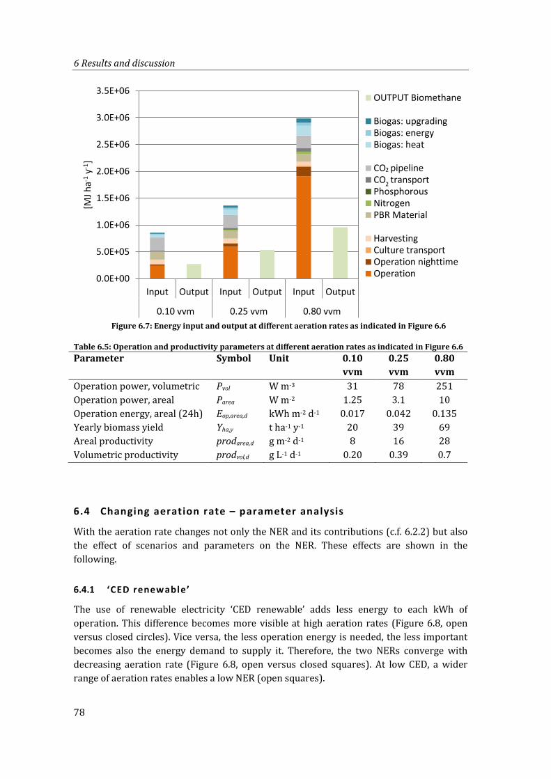
6 Results and discussion
78
Figure 6.7: Energy input and output at different aeration rates as indicated in Figure 6.6
Table 6.5: Operation and productivity parameters at different aeration rates as indicated in Figure 6.6 Parameter Symbol Unit 0.10
vvm 0.25 vvm
0.80 vvm
Operation power, volumetric Pvol W m-3 31 78 251 Operation power, areal Parea W m-2 1.25 3.1 10 Operation energy, areal (24h) Eop,area,d kWh m-2 d-1 0.017 0.042 0.135 Yearly biomass yield Yha,y t ha-1 y-1 20 39 69 Areal productivity prodarea,d g m-2 d-1 8 16 28 Volumetric productivity prodvol,d g L-1 d-1 0.20 0.39 0.7
6.4 Changing aeration rate – parameter analysis
With the aeration rate changes not only the NER and its contributions (c.f. 6.2.2) but also the effect of scenarios and parameters on the NER. These effects are shown in the following.
6.4.1 ‘CED renewable’
The use of renewable electricity ‘CED renewable’ adds less energy to each kWh of operation. This difference becomes more visible at high aeration rates (Figure 6.8, open versus closed circles). Vice versa, the less operation energy is needed, the less important becomes also the energy demand to supply it. Therefore, the two NERs converge with decreasing aeration rate (Figure 6.8, open versus closed squares). At low CED, a wider range of aeration rates enables a low NER (open squares).
0.0E+00
5.0E+05
1.0E+06
1.5E+06
2.0E+06
2.5E+06
3.0E+06
3.5E+06
Input Output Input Output Input Output
0.10 vvm 0.25 vvm 0.80 vvm
[MJ h
a-1y-1
]OUTPUT Biomethane
Biogas: upgradingBiogas: energyBiogas: heat
CO pipelineCO transportPhosphorousNitrogenPBR Material
HarvestingCulture transportOperation nighttimeOperation
2
2
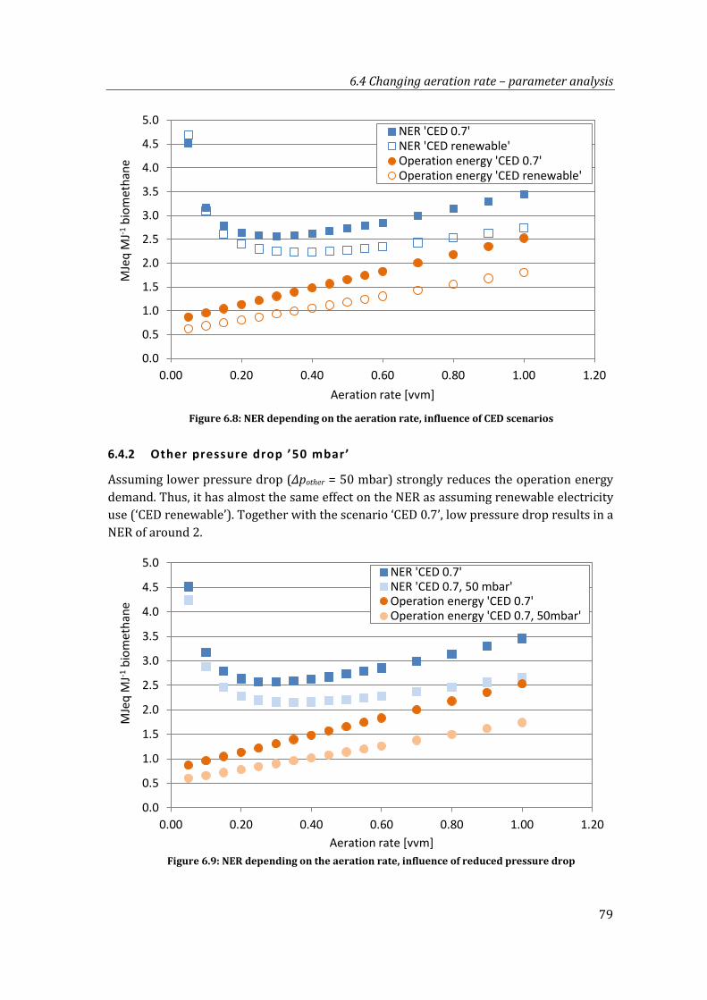
6.4 Changing aeration rate – parameter analysis
79
Figure 6.8: NER depending on the aeration rate, influence of CED scenarios
6.4.2 Other pressure drop ’50 mbar’
Assuming lower pressure drop (Δpother = 50 mbar) strongly reduces the operation energy demand. Thus, it has almost the same effect on the NER as assuming renewable electricity use (‘CED renewable’). Together with the scenario ‘CED 0.7’, low pressure drop results in a NER of around 2.
Figure 6.9: NER depending on the aeration rate, influence of reduced pressure drop
0.0
0.5
1.0
1.5
2.0
2.5
3.0
3.5
4.0
4.5
5.0
0.00 0.20 0.40 0.60 0.80 1.00 1.20
MJe
q M
J-1bi
omet
hane
Aeration rate [vvm]
NER 'CED 0.7'NER 'CED renewable'Operation energy 'CED 0.7'Operation energy 'CED renewable'
0.0
0.5
1.0
1.5
2.0
2.5
3.0
3.5
4.0
4.5
5.0
0.00 0.20 0.40 0.60 0.80 1.00 1.20
MJe
q M
J-1bi
omet
hane
Aeration rate [vvm]
NER 'CED 0.7'NER 'CED 0.7, 50 mbar'Operation energy 'CED 0.7'Operation energy 'CED 0.7, 50mbar'
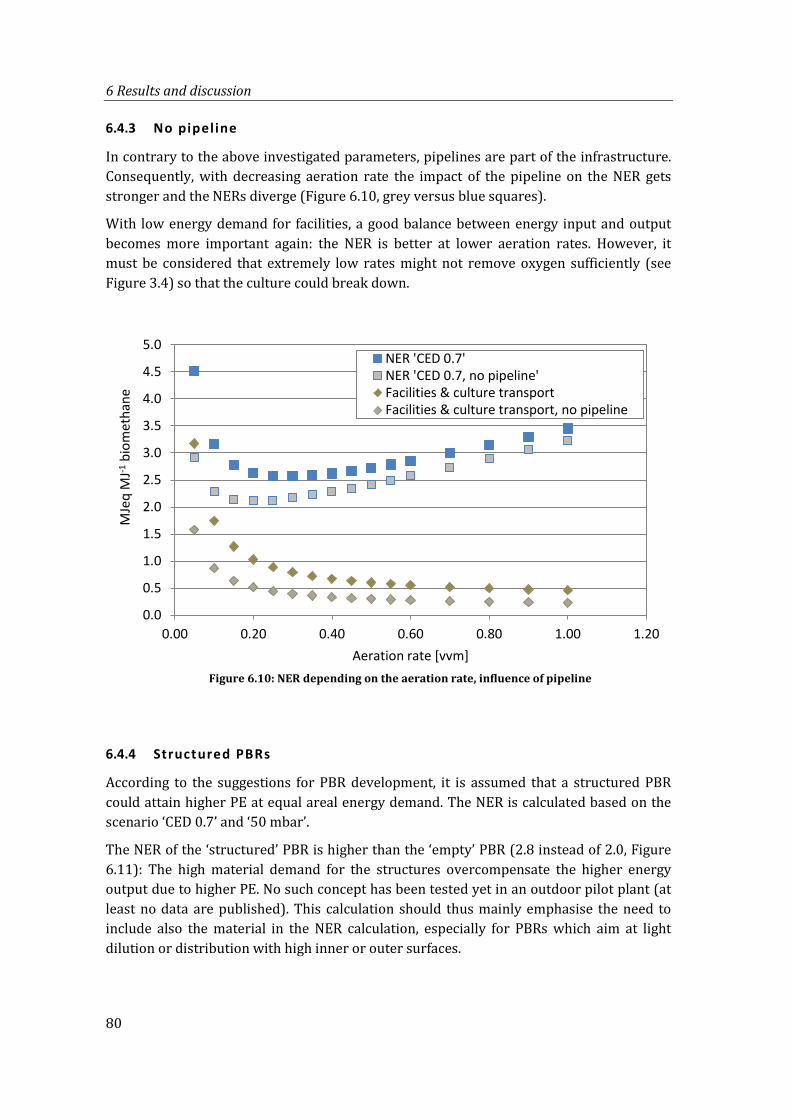
6 Results and discussion
80
6.4.3 No pipeline
In contrary to the above investigated parameters, pipelines are part of the infrastructure. Consequently, with decreasing aeration rate the impact of the pipeline on the NER gets stronger and the NERs diverge (Figure 6.10, grey versus blue squares).
With low energy demand for facilities, a good balance between energy input and output becomes more important again: the NER is better at lower aeration rates. However, it must be considered that extremely low rates might not remove oxygen sufficiently (see Figure 3.4) so that the culture could break down.
Figure 6.10: NER depending on the aeration rate, influence of pipeline
6.4.4 Structured PBRs
According to the suggestions for PBR development, it is assumed that a structured PBR could attain higher PE at equal areal energy demand. The NER is calculated based on the scenario ‘CED 0.7’ and ‘50 mbar’.
The NER of the ‘structured’ PBR is higher than the ‘empty’ PBR (2.8 instead of 2.0, Figure 6.11): The high material demand for the structures overcompensate the higher energy output due to higher PE. No such concept has been tested yet in an outdoor pilot plant (at least no data are published). This calculation should thus mainly emphasise the need to include also the material in the NER calculation, especially for PBRs which aim at light dilution or distribution with high inner or outer surfaces.
0.0
0.5
1.0
1.5
2.0
2.5
3.0
3.5
4.0
4.5
5.0
0.00 0.20 0.40 0.60 0.80 1.00 1.20
MJe
q M
J-1bi
omet
hane
Aeration rate [vvm]
NER 'CED 0.7'NER 'CED 0.7, no pipeline'Facilities & culture transportFacilities & culture transport, no pipeline
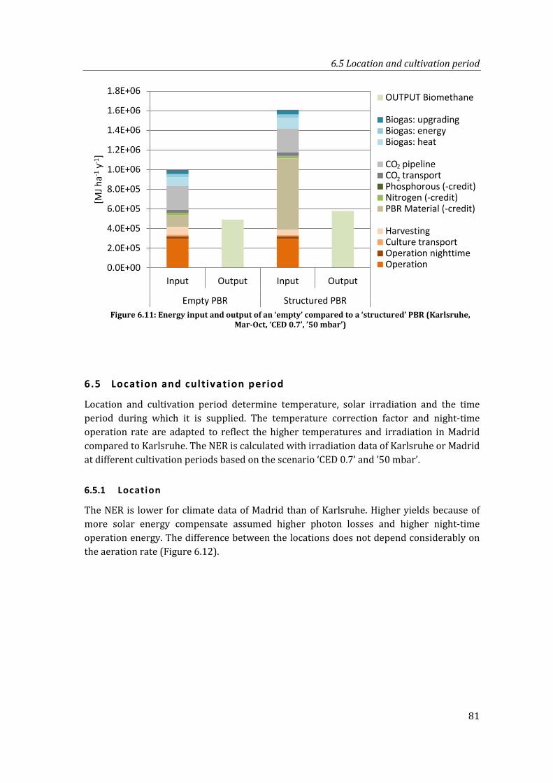
6.5 Location and cultivation period
81
Figure 6.11: Energy input and output of an ‘empty’ compared to a ‘structured’ PBR (Karlsruhe,
Mar-Oct, ‘CED 0.7’, ’50 mbar’)
6.5 Location and cultivation period
Location and cultivation period determine temperature, solar irradiation and the time period during which it is supplied. The temperature correction factor and night-time operation rate are adapted to reflect the higher temperatures and irradiation in Madrid compared to Karlsruhe. The NER is calculated with irradiation data of Karlsruhe or Madrid at different cultivation periods based on the scenario ‘CED 0.7’ and ’50 mbar’.
6.5.1 Location
The NER is lower for climate data of Madrid than of Karlsruhe. Higher yields because of more solar energy compensate assumed higher photon losses and higher night-time operation energy. The difference between the locations does not depend considerably on the aeration rate (Figure 6.12).
0.0E+00
2.0E+05
4.0E+05
6.0E+05
8.0E+05
1.0E+06
1.2E+06
1.4E+06
1.6E+06
1.8E+06
Input Output Input Output
Empty PBR Structured PBR
[MJ h
a-1y-1
]OUTPUT Biomethane
Biogas: upgradingBiogas: energyBiogas: heat
CO pipelineCO transportPhosphorous (-credit)Nitrogen (-credit)PBR Material (-credit)
HarvestingCulture transportOperation nighttimeOperation
2
2
6 Results and discussion
82
Figure 6.12: NER depending on the aeration rate – comparison Karlsruhe and Madrid (Mar-Oct,
‘CED 0.7’, ’50 mbar’)
This result is based on the estimated photon loss for passive temperature control. If cultivation in Madrid required more sunlight protection – more photons would be lost and the yield would sink – the NERs would converge. Furthermore, the assumption that the PE does not depend on the light intensity is more advantageous for climate data of Madrid than of Karlsruhe. In Madrid (in 2012), the light intensity was above 500 µmol m-2 s-1 in over 75% of sunlight hours (60% of time Karlsruhe) (c.f. Annex, Figure A.3). Moreover, photoinhibition and overheating – and thus culture breakdown due to high light intensities is more likely in Madrid where the light intensity is more often above 1800 µmol m-2 s-1 (c.f. Annex, Figure A.4).
In general, countries with more sunlight have potential higher biomass yields (see 3.1.2). At the same time, greater efforts are required to provide optimal growth temperature and light intensity. To compare different locations, it would be necessary to consider these trade-offs in greater detail.
Notably, the NER changes not as much as the areal productivity. For example, at 0.6 vvm the areal productivity and thus the biomethane output increases by almost a third (Figure 6.13). Yet, the NER sinks only from 2.2 to 1.9 since a higher biomass output requires also more energy for upstream and downstream processes.
0.00.51.01.52.02.53.03.54.04.5
0.00 0.20 0.40 0.60 0.80 1.00 1.20
NER
Aeration rate [vvm]
KarlsruheMadrid
6.5 Location and cultivation period
83
Figure 6.13: Energy inputs and outputs for cultivation in Karlsruhe and Madrid at 0.6 vvm
(Mar-Oct, ‘CED 0.7’, ’50 mbar’)
6.5.2 Cultivation period
Shortening the cultivation time (beginning from a year-round cultivation) has a similar effect on the NER as decreasing the aeration rate: The NER initially sinks and then increases again more steeply (Figure 6.14). The effect is similar in Madrid (Figure 6.15). The reason is in that case however not the ratio of vvm to PE (see 6.3) which remains constant, but the light intensity: with less sunlight, the same PE results in lower yields (c.f. equation (13)). Winter days do not provide much sunlight, but the PBR must be operated nevertheless; thus cultivating microalgae during the whole year is less energy-efficient than cultivating them in months with high solar irradiation (see also Annex, Figure A.2). However, analogue to a very low aeration rate, a very short cultivation time results in too few biomass so that the share of infrastructure on the NER increases and the NER rises again.
Table 6.6 shows for example, that for a cultivation period between May and August, more biomass is produced per day (19 versus 12 g m-2 d-1) but less during the whole year (24 versus 43 t ha-1 y-1).
Preconditions for this effect are that (a) the PE does not depend on the light intensity and (b) that the culture does not break down due to overheating (see also discussion of the previous section).
0.0E+00
5.0E+05
1.0E+06
1.5E+06
2.0E+06
2.5E+06
Input Output Input Output
Karlsruhe Madrid
[MJ h
a-1y-1
]OUTPUT Biomethane
Biogas: upgradingBiogas: energyBiogas: heat
CO pipelineCO transportPhosphorousNitrogenPBR Material
HarvestingCulture transportOperation nighttimeOperation
2
2
6 Results and discussion
84
Figure 6.14: NER depending on the cultivation period (Karlsruhe, 0.25 vvm ‘CED 0.7, 50 mbar’)
Table 6.6: Operation and productivity parameters at different cultivation times as indicated in Figure 6.14 Parameter Symbol Unit Jan-Dec May-Aug Operation power, volumetric Pvol W m-3 54 54 Operation power, areal Parea W m-2 2.2 2.2 Operation energy, areal (24h) Eop,area,d kWh m-2 d-1 0.025 0.031 Yearly biomass yield Yha,y t ha-1 y-1 43 24 Areal productivity prodarea,d g m-2 d-1 12 19 Volumetric productivity prodvol,d g L-1 d-1 0.3 0.5
Figure 6.15: NER depending on the cultivation period (Madrid, 0.25 vvm ‘CED 0.7, 50 mbar’)
0.0
0.5
1.0
1.5
2.0
2.5
3.0
3.5
4.0
0 1 2 3 4 5 6 7
[MJe
q M
J-1bi
omet
hane
]NER (KA, 0.25 vvm, CED 0.7, 50 mbar)Facilities & culture transportOperation energyBiomass related ressources
0.0
0.5
1.0
1.5
2.0
2.5
3.0
0 1 2 3 4 5 6 7
[MJe
q M
J-1bi
omet
hane
]
NER (MA, 0.25 vvm, CED 0.7, 50 mbar)Facilities & culture transportOperation energyBiomass related ressources
Jan-Dec Feb-Nov Mar-Oct Apr-Sept May-Aug Jun-Jul
Jan-Dec Feb-Nov Mar-Oct Apr-Sept May-Aug Jun-Jul
6.6 Summary of findings and definition of best case
85
Table 6.7: Operation and productivity parameters at different cultivation times as indicated in Figure 6.15 Parameter Symbol Unit Jan-Dec May-Aug Operation power, volumetric Pvol W m-3 54 54 Operation power, areal Parea W m-2 2.2 2.2 Operation energy, areal (24h) Eop,area,d kWh m-2 d-1 0.029 0.032 Yearly biomass yield Yha,y t ha-1 y-1 60 31 Areal productivity prodarea,d g m-2 d-1 16 25 Volumetric productivity prodvol,d g L-1 d-1 0.41 0.62
Interaction of cultivation period an aeration rate
The optimal cultivation period for a low NER depends also on the aeration rate (Figure 6.14): At very high rates (dark blue squares), microalgae cultivation is only energy-efficient in months that provide much solar energy in a short time. At very low rates (light blue squares), it is better to cultivate microalgae during the whole year. At a good balance between aeration rate and biomass yield (middle blue squares), the cultivation period has a relatively low effect on the NER.
Figure 6.16: NER at different cultivation periods and aeration rates (Karlsruhe, ‘CED 0.7, 50 mbar’)
6.6 Summary of f indings and definition of best case
Due to the correlated parameters, the lowest NER is attained at low aeration rates which are more energy-efficient. Nevertheless, because of the energy demand for infrastructure and the resources needed to produce and process the biomass, the lowest NER remains around two.
0.0
2.0
4.0
6.0
8.0
10.0
12.0
0 1 2 3 4 5 6 7
NER
KA 4.0 vvmKA 0.25 vvmKA 0.05 vvm
Jan-Dec Feb-Nov Mar-Oct Apr-Sept May-Aug Jun-Jul
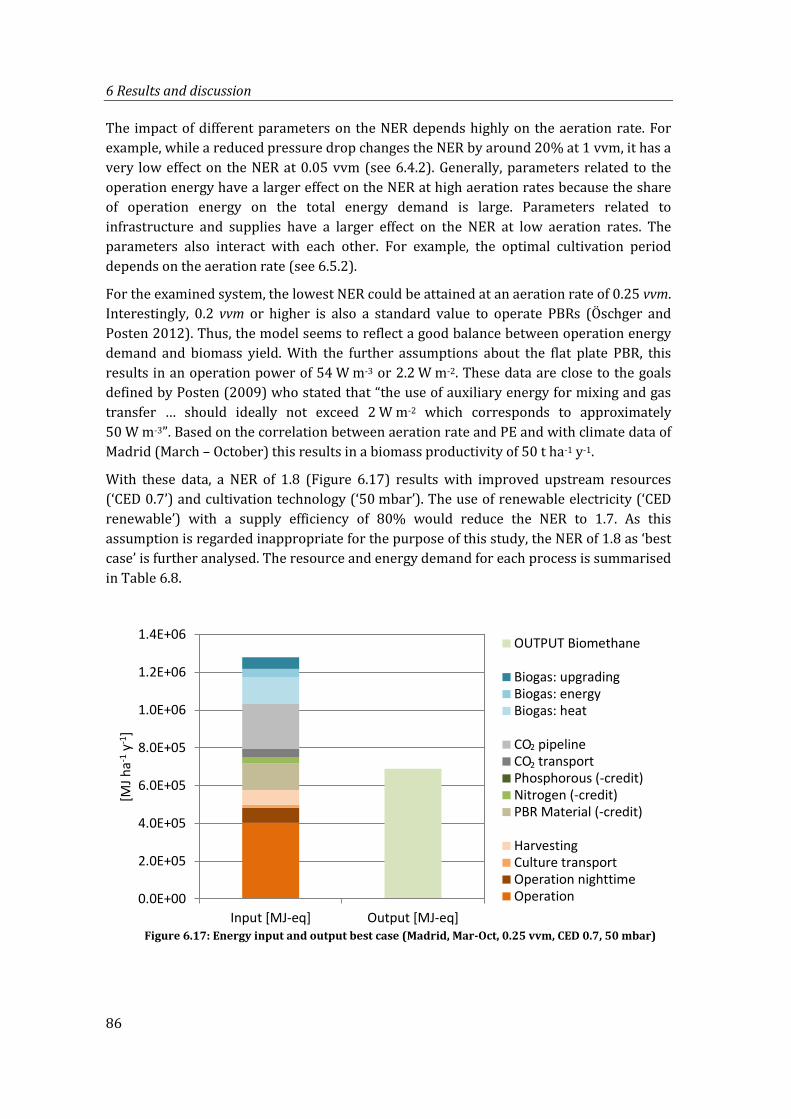
6 Results and discussion
86
The impact of different parameters on the NER depends highly on the aeration rate. For example, while a reduced pressure drop changes the NER by around 20% at 1 vvm, it has a very low effect on the NER at 0.05 vvm (see 6.4.2). Generally, parameters related to the operation energy have a larger effect on the NER at high aeration rates because the share of operation energy on the total energy demand is large. Parameters related to infrastructure and supplies have a larger effect on the NER at low aeration rates. The parameters also interact with each other. For example, the optimal cultivation period depends on the aeration rate (see 6.5.2).
For the examined system, the lowest NER could be attained at an aeration rate of 0.25 vvm. Interestingly, 0.2 vvm or higher is also a standard value to operate PBRs (Öschger and Posten 2012). Thus, the model seems to reflect a good balance between operation energy demand and biomass yield. With the further assumptions about the flat plate PBR, this results in an operation power of 54 W m-3 or 2.2 W m-2. These data are close to the goals defined by Posten (2009) who stated that “the use of auxiliary energy for mixing and gas transfer … should ideally not exceed 2 W m-2 which corresponds to approximately 50 W m-3”. Based on the correlation between aeration rate and PE and with climate data of Madrid (March – October) this results in a biomass productivity of 50 t ha-1 y-1.
With these data, a NER of 1.8 (Figure 6.17) results with improved upstream resources (‘CED 0.7’) and cultivation technology (‘50 mbar’). The use of renewable electricity (‘CED renewable’) with a supply efficiency of 80% would reduce the NER to 1.7. As this assumption is regarded inappropriate for the purpose of this study, the NER of 1.8 as ‘best case’ is further analysed. The resource and energy demand for each process is summarised in Table 6.8.
Figure 6.17: Energy input and output best case (Madrid, Mar-Oct, 0.25 vvm, CED 0.7, 50 mbar)
0.0E+00
2.0E+05
4.0E+05
6.0E+05
8.0E+05
1.0E+06
1.2E+06
1.4E+06
Input [MJ-eq] Output [MJ-eq]
[MJ h
a-1y-1
]
OUTPUT Biomethane
Biogas: upgradingBiogas: energyBiogas: heat
CO pipelineCO transportPhosphorous (-credit)Nitrogen (-credit)PBR Material (-credit)
HarvestingCulture transportOperation nighttimeOperation
2
2
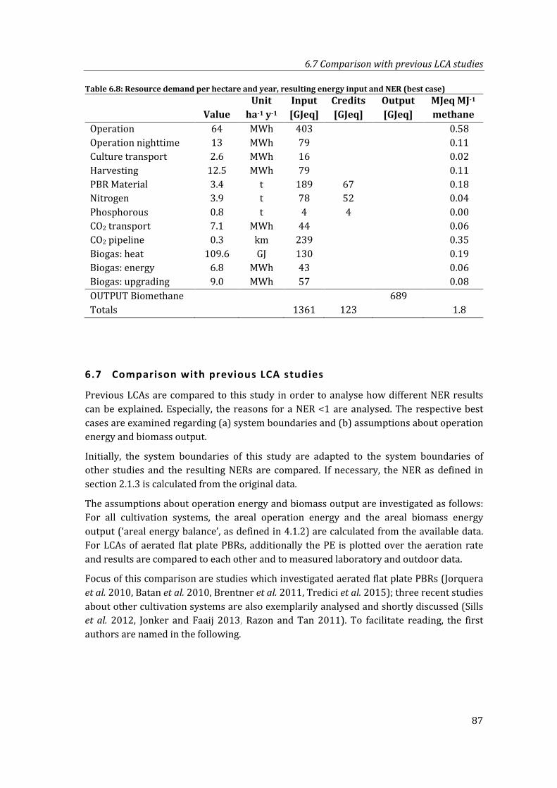
6.7 Comparison with previous LCA studies
87
Table 6.8: Resource demand per hectare and year, resulting energy input and NER (best case)
Value Unit
ha-1 y-1 Input [GJeq]
Credits [GJeq]
Output [GJeq]
MJeq MJ-1 methane
Operation 64 MWh 403 0.58 Operation nighttime 13 MWh 79 0.11 Culture transport 2.6 MWh 16 0.02 Harvesting 12.5 MWh 79 0.11 PBR Material 3.4 t 189 67 0.18 Nitrogen 3.9 t 78 52 0.04 Phosphorous 0.8 t 4 4 0.00 CO2 transport 7.1 MWh 44 0.06 CO2 pipeline 0.3 km 239 0.35 Biogas: heat 109.6 GJ 130 0.19 Biogas: energy 6.8 MWh 43 0.06 Biogas: upgrading 9.0 MWh 57 0.08 OUTPUT Biomethane 689 Totals 1361 123 1.8
6.7 Comparison with previous LCA studies
Previous LCAs are compared to this study in order to analyse how different NER results can be explained. Especially, the reasons for a NER <1 are analysed. The respective best cases are examined regarding (a) system boundaries and (b) assumptions about operation energy and biomass output.
Initially, the system boundaries of this study are adapted to the system boundaries of other studies and the resulting NERs are compared. If necessary, the NER as defined in section 2.1.3 is calculated from the original data.
The assumptions about operation energy and biomass output are investigated as follows: For all cultivation systems, the areal operation energy and the areal biomass energy output (‘areal energy balance’, as defined in 4.1.2) are calculated from the available data. For LCAs of aerated flat plate PBRs, additionally the PE is plotted over the aeration rate and results are compared to each other and to measured laboratory and outdoor data.
Focus of this comparison are studies which investigated aerated flat plate PBRs (Jorquera et al. 2010, Batan et al. 2010, Brentner et al. 2011, Tredici et al. 2015); three recent studies about other cultivation systems are also exemplarily analysed and shortly discussed (Sills et al. 2012, Jonker and Faaij 2013, Razon and Tan 2011). To facilitate reading, the first authors are named in the following.
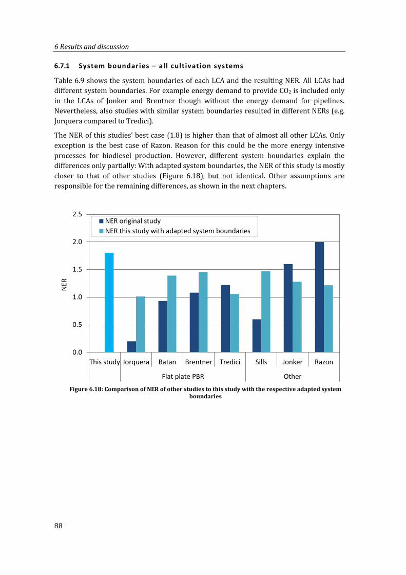
6 Results and discussion
88
6.7.1 System boundaries – al l cultivation systems
Table 6.9 shows the system boundaries of each LCA and the resulting NER. All LCAs had different system boundaries. For example energy demand to provide CO2 is included only in the LCAs of Jonker and Brentner though without the energy demand for pipelines. Nevertheless, also studies with similar system boundaries resulted in different NERs (e.g. Jorquera compared to Tredici).
The NER of this studies’ best case (1.8) is higher than that of almost all other LCAs. Only exception is the best case of Razon. Reason for this could be the more energy intensive processes for biodiesel production. However, different system boundaries explain the differences only partially: With adapted system boundaries, the NER of this study is mostly closer to that of other studies (Figure 6.18), but not identical. Other assumptions are responsible for the remaining differences, as shown in the next chapters.
Figure 6.18: Comparison of NER of other studies to this study with the respective adapted system
boundaries
0.0
0.5
1.0
1.5
2.0
2.5
This study Jorquera Batan Brentner Tredici Sills Jonker Razon
Flat plate PBR Other
NER
NER original studyNER this study with adapted system boundaries
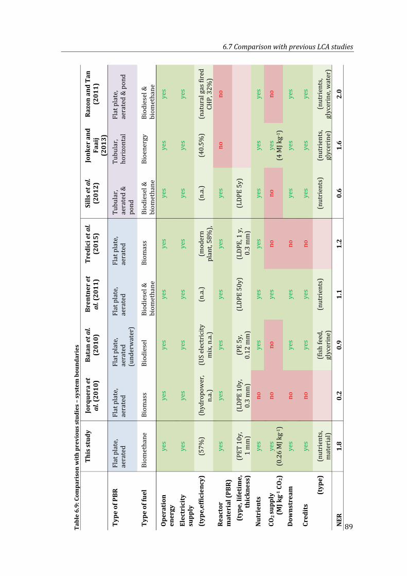
6.7 Comparison with previous LCA studies
89 Tabl
e 6.
9: C
ompa
riso
n w
ith
prev
ious
stu
dies
– s
yste
m b
ound
arie
s
Th
is s
tudy
Jo
rque
ra e
t al
. (20
10)
Bata
n et
al.
(201
0)
Bren
tner
et
al. (
2011
) Tr
edic
i et a
l. (2
015)
Si
lls e
t al.
(201
2)
Jonk
er a
nd
Faai
j (2
013)
Razo
n an
d Ta
n (2
011)
Type
of P
BR
Flat
pla
te,
aera
ted
Flat
pla
te,
aera
ted
Flat
pla
te,
aera
ted
(und
erw
ater
)
Flat
pla
te,
aera
ted
Flat
pla
te,
aera
ted
Tubu
lar,
aera
ted
&
pond
Tubu
lar,
hori
zont
al
Flat
pla
te,
aera
ted
& p
ond
Type
of f
uel
Biom
etha
ne
Biom
ass
Biod
iese
l Bi
odie
sel &
bi
omet
hane
Bi
omas
s Bi
odie
sel &
bi
omet
hane
Bi
oene
rgy
Biod
iese
l &
biom
etha
ne
Ope
rati
on
ener
gy
yes
yes
yes
yes
yes
yes
yes
yes
Elec
tric
ity
supp
ly
yes
yes
yes
yes
yes
yes
yes
yes
(typ
e,ef
ficie
ncy)
(5
7%)
(hyd
ropo
wer
, n.
a.)
(US
elec
tric
ity
mix
, n.a
.) (n
.a.)
(mod
ern
plan
t, 58
%),
(n.a
.) (4
0.5%
) (n
atur
al g
as fi
red
CHP,
32%
) Re
acto
r m
ater
ial (
PBR)
ye
s ye
s ye
s ye
s ye
s ye
s no
no
(typ
e, li
feti
me,
th
ickn
ess)
(P
ET 1
0y,
1 m
m)
(LDP
E 10
y,
0.3
mm
) (P
E 5y
, 0.
12 m
m)
(LDP
E 50
y)
(LDP
E, 1
y,
0.3
mm
) (L
DPE
5y)
Nut
rien
ts
yes
no
yes
yes
yes
yes
yes
yes
CO2
supp
ly
(MJ k
g-1 C
O2)
ye
s (0
.26
MJ k
g-1)
no
no
yes
no
no
yes
(4 M
J kg-1
) no
Dow
nstr
eam
ye
s no
ye
s ye
s no
ye
s ye
s ye
s
Cred
its
yes
no
yes
yes
no
yes
yes
yes
(typ
e)
(nut
rien
ts,
mat
eria
l)
(fis
h fe
ed,
glyc
erin
e)
(nut
rien
ts)
(n
utri
ents
) (n
utri
ents
, gl
ycer
ine)
(n
utri
ents
, gl
ycer
ine,
wat
er)
NER
1.
8 0.
2 0.
9 1.
1 1.
2 0.
6 1.
6 2.
0
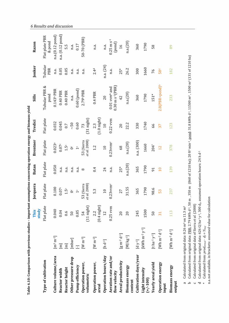
6 Results and discussion
90
Tabl
e 6.
10: C
ompa
riso
n w
ith
prev
ious
stu
dies
– im
port
ant a
ssum
ptio
ns c
once
rnin
g op
erat
ion
ener
gy a
nd b
iom
ass
yiel
d
Th
is
stud
y Jo
rque
ra
Bata
n Br
entn
er
Tred
ici
Sills
Jo
nker
Ra
zon
Type
of c
ulti
vati
on
Fl
at p
late
Fl
at p
late
Fl
at p
late
Fl
at p
late
Fl
at p
late
Tu
bula
r PBR
&
pond
Tu
bula
r PB
R Fl
at p
late
PBR
&
pon
d Cu
ltur
e vo
lum
e/ar
ea
[m3 m
-2]
0.04
0 0.
100
0.05
0 0.
023a
0.03
2 0.
143b P
BR
n.a.
n.
a.(0
.12
pond
) Re
acto
r w
idth
[m
] 0.
04
0.07
c n.
a.
0.07
c 0.
045
0.40
PBR
0.
05
n.a.
(0.1
2 po
nd)
Reac
tor
heig
ht
[m]
0.6
1.5c
n.a.
1.
5c 0.
7 0.
40 P
BR
0.05
5.
5 O
ther
pre
ssur
e dr
op
[mba
r]
50
0c n.
a.
0c ~
50
n.a.
n.
a.
n.a.
Pu
mp
effic
ienc
y [-
] 0.
85
1c n.
a.
1c 0.
60
0.60
(pon
d)
n.a.
0.
17
Ope
rati
on p
ower
, vo
lum
etri
c [W
m-3
] 54
(1
1 ni
ght)
53
(Sie
rra
et a
l. 20
08)
8 53
(Sie
rra
et a
l. 20
08)
73
(31
nigh
t)
2.79
b PB
R n.
a.
50-7
0 (P
BR)
Ope
rati
on p
ower
, ar
eal
[W m
-2]
2.2
(0
.4 n
ight
) 5.
3 0.
4
1.2
2.3
(1
.0 n
ight
) 0.
4 PB
R
2.4d
n.a.
Ope
rati
on h
ours
/day
[h
d-1
] 12
10
24
10
10
20
n.
a. (2
4)
n.a.
Ae
rati
on r
ate
and/
or
flow
vel
ocit
y
0.25
vvm
0.
23vv
mc
n.a.
0.
23vv
mc
0.22
vvm
0.
01 v
vmb a
nd
0.30
m s-1
(PBR
) n.
a.
0.25
m s-1
(p
ond)
Ar
eal p
rodu
ctiv
ity
[g
m-2
d-1
] 20
27
25
* 68
20
42
25
* 16
Biom
ass
ener
gy
cont
ent
[MJ k
g-1]
20
31.5
5 n.
a.(2
0)
n.a.
(20)
22
.2
n.a.
(20)
26
.2
n.a.
(20)
Cult
ivat
ion
days
/yea
r [d
y-1
] 24
5 36
5 36
5 n.
a. (3
00)
330
360
300
360
Ligh
t int
ensi
ty
(+/-
100)
[k
Wh
m-2
y-1
] 15
00
1790
17
90
1660
17
40
1790
16
60
1790
Year
ly a
real
yie
ld
[t h
a-1 y
-1]
50
98.6
91
20
4* 66
15
1*
76
58
Ope
rati
on e
nerg
y in
put
[Wh
m-2
d-1
] 31
53
10
12
37
2.
8(PB
R+po
nd)b
58d
Biom
ass
ener
gy
outp
ut
[Wh
m-2
d-1
] 11
3 23
7 13
9 37
8 12
3 23
3 18
2 89
aCa
lcul
ated
from
ori
gina
l dat
a: 0
.26
m3 o
n 11
.3 m
2 b
Calc
ulat
ed fr
om o
rigi
nal d
ata:
PBR
: 2.7
9 kW
h d-
1 , 50
m³,
350
m² (
860
of 1
210
ha);
20 ft
3 min
-1, p
ond:
31.
8 kW
h d-
1 , 11
500
m2 ,
150
0 m
3 (13
1 of
121
0 ha
) c
Calc
ulat
ed fr
om o
rigi
nal d
ata
of S
ierr
a et
al.
(200
8)
dCa
lcul
ated
from
ori
gina
l dat
a: 6
26 G
J ha-
1 y-
1 , 30
0 d y
, ass
umed
ope
ratio
n ho
urs:
24
h d-
1 *
Calc
ulat
ed fr
om: p
rod a
rea,
d ⋅ d
y = Y
ha,y
n.a.
not
ava
ilabl
e, in
bra
cket
s: a
ssum
ed v
alue
for c
alcu
latio
n
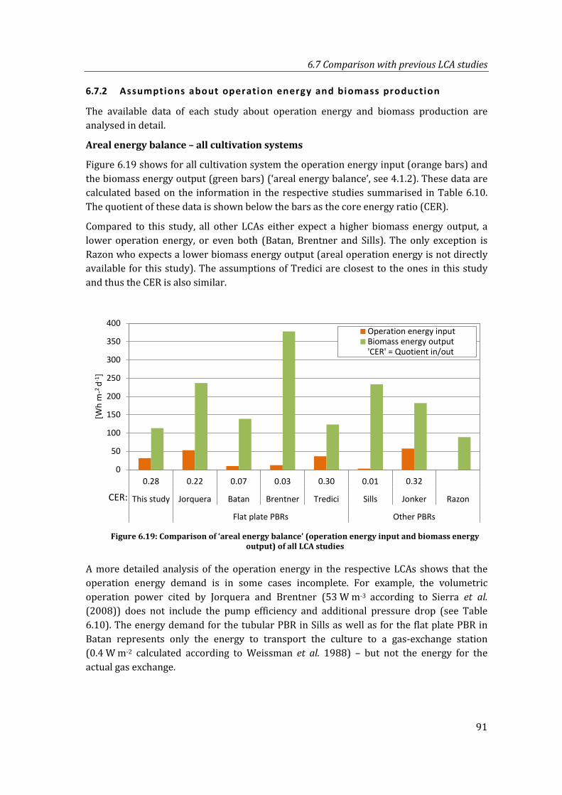
6.7 Comparison with previous LCA studies
91
6.7.2 Assumptions about operation energy and biomass production
The available data of each study about operation energy and biomass production are analysed in detail.
Areal energy balance – all cultivation systems
Figure 6.19 shows for all cultivation system the operation energy input (orange bars) and the biomass energy output (green bars) (‘areal energy balance’, see 4.1.2). These data are calculated based on the information in the respective studies summarised in Table 6.10. The quotient of these data is shown below the bars as the core energy ratio (CER).
Compared to this study, all other LCAs either expect a higher biomass energy output, a lower operation energy, or even both (Batan, Brentner and Sills). The only exception is Razon who expects a lower biomass energy output (areal operation energy is not directly available for this study). The assumptions of Tredici are closest to the ones in this study and thus the CER is also similar.
Figure 6.19: Comparison of ‘areal energy balance’ (operation energy input and biomass energy
output) of all LCA studies
A more detailed analysis of the operation energy in the respective LCAs shows that the operation energy demand is in some cases incomplete. For example, the volumetric operation power cited by Jorquera and Brentner (53 W m-3 according to Sierra et al. (2008)) does not include the pump efficiency and additional pressure drop (see Table 6.10). The energy demand for the tubular PBR in Sills as well as for the flat plate PBR in Batan represents only the energy to transport the culture to a gas-exchange station (0.4 W m-2 calculated according to Weissman et al. 1988) – but not the energy for the actual gas exchange.
0.28 0.22 0.07 0.03 0.30 0.01 0.320
50
100
150
200
250
300
350
400
.
This study Jorquera Batan Brentner Tredici Sills Jonker Razon
Flat plate PBRs Other PBRs
[Wh
m-2
d-1]
Operation energy inputBiomass energy output'CER' = Quotient in/out
CER:
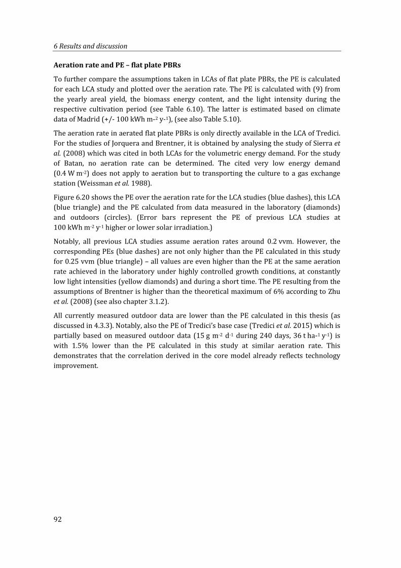
6 Results and discussion
92
Aeration rate and PE – flat plate PBRs
To further compare the assumptions taken in LCAs of flat plate PBRs, the PE is calculated for each LCA study and plotted over the aeration rate. The PE is calculated with (9) from the yearly areal yield, the biomass energy content, and the light intensity during the respective cultivation period (see Table 6.10). The latter is estimated based on climate data of Madrid (+/- 100 kWh m-2 y-1), (see also Table 5.10).
The aeration rate in aerated flat plate PBRs is only directly available in the LCA of Tredici. For the studies of Jorquera and Brentner, it is obtained by analysing the study of Sierra et al. (2008) which was cited in both LCAs for the volumetric energy demand. For the study of Batan, no aeration rate can be determined. The cited very low energy demand (0.4 W m-2) does not apply to aeration but to transporting the culture to a gas exchange station (Weissman et al. 1988).
Figure 6.20 shows the PE over the aeration rate for the LCA studies (blue dashes), this LCA (blue triangle) and the PE calculated from data measured in the laboratory (diamonds) and outdoors (circles). (Error bars represent the PE of previous LCA studies at 100 kWh m-2 y-1 higher or lower solar irradiation.)
Notably, all previous LCA studies assume aeration rates around 0.2 vvm. However, the corresponding PEs (blue dashes) are not only higher than the PE calculated in this study for 0.25 vvm (blue triangle) – all values are even higher than the PE at the same aeration rate achieved in the laboratory under highly controlled growth conditions, at constantly low light intensities (yellow diamonds) and during a short time. The PE resulting from the assumptions of Brentner is higher than the theoretical maximum of 6% according to Zhu et al. (2008) (see also chapter 3.1.2).
All currently measured outdoor data are lower than the PE calculated in this thesis (as discussed in 4.3.3). Notably, also the PE of Tredici’s base case (Tredici et al. 2015) which is partially based on measured outdoor data (15 g m-2 d-1 during 240 days, 36 t ha-1 y-1) is with 1.5% lower than the PE calculated in this study at similar aeration rate. This demonstrates that the correlation derived in the core model already reflects technology improvement.
6.7 Comparison with previous LCA studies
93
Figure 6.20: PE over vvm for aerated flat plate PBRs, comparison of LCA assumptions with
laboratory and outdoor data
6.7.3 Potential improvements due to genetical ly modified algae?
As many other studies assumed a better relation between aeration rate and PE, the question is whether or how this can be achieved. The correlation between aeration rate and PE is due to mass transfer rates and light management (see 4.1.1). Could genetically modified algae (GMA) decrease the energy demand for high mass transfer rates and good light management?
Genetically modified algae cannot save the energy for mixing: all algae need high mass transfer rates for fast growth. Neither is it possible to accelerate the growth-limiting dark reactions of algae: they involve too many enzymes and metabolic processes (see 3.1.1). Even if it was possible to accelerate carbon fixation, one of the following enzymes in the complex cascade of dark reactions would still limit microalgae growth (Williams and Laurens 2010).
0.0%
1.0%
2.0%
3.0%
4.0%
5.0%
6.0%
7.0%
8.0%
0 1 2 3 4 5
PE [%
]
Aeration rate (vvm) [m3 m-3 min-1]
This study
LCA assumptions (flat plate)
Laboratory (500 )
Laboratory (900
Laboratory (1800
Outdoor data
µmol m-2 s-1
µmol m-2 s-1)
µmol m-2 s-1)
Hu 1996
Rodolfi 2009
Quinn 2012
Tredici
Brentner
Jorquera
Batan
6 Results and discussion
94
Due to the above described limitations, most of the research focusses on improved light management. In this thesis, it is assumed that algae can use high light intensities as efficiently as low (see 4.4) to calculate the PE depending on the aeration rate.
One suggestion to genetically engineer algae for better light use is for example to ‘lock’ microalgae in the state where they are adapted to high light (see also 3.1.3 f). In theory, “if the chlorophyll content is reduced, a greater number of photons are delivered to the deeper parts of the culture” (Williams and Laurens 2011). This could save mixing energy for light management – however, high mass transfer rates and gas exchange must be maintained. Algae that cannot adapt to changing light intensities any more can also be a disadvantage for outdoor cultures (Tredici 2010, Williams and Laurens 2010). Furthermore, energy is needed “to control light conditions in bioreactors” (Mussgnug et al. 2007). This might offset savings due to higher PE.
Cultivating GMA brings along disadvantages. For example, the genetically modified green algae Chlamydomonas reinhardtii (Stm6) grows only half as fast as the wild type (wt13) (1.2 d-1 (Franz et al. 2012) versus 2.5 d-1 (Jacobi et al. 2012)). This might also affect the PE. Apart from that, GMA tend to re-mutate and are poorly competitive with other species (Williams and Laurens 2011). It is thus questionable whether GMA can solve the problems of energy-efficient microalgae mass cultivation.
6.7.4 Potential improvements due to other cultivation systems?
Of the other recent studies which are exemplarily analysed in this thesis, only Sills et al. (2012) resulted in a NER below one in their best case. The authors themselves mentioned the limitation that they did not correlate important process parameters. In the following, it is shortly discussed to what extent other cultivation systems could improve the relation between energy demand and biomass energy output.
Tubular photobioreactors
Tubular PBRs need turbulent flow conditions to provide high mass transfer rates and to “avoid that the cells stagnate in the dark interior of a tube” (Acién et al. 2013). Turbulent flow conditions come along with high friction losses and thus a high energy demand (c.f. equation (22)), especially in long PBRs required on large scale. Furthermore in tubes, oxygen accumulates quickly and carbon is often limited so that many gas exchange station are required (Acién et al. 2013, Tredici 2003). Hulatt and Thomas (2011) experimented on a tubular reactor and found that it “consumed 15 times more energy in circulating the culture than it produced as biomass” (CER of 15). It has thus been proposed that microalgae cultivation in tubular PBRs requires more energy than in flat plate PBRs (Lehr and Posten 2009, Tredici and Materassi 1992, Hulatt and Thomas 2011).
Open ponds
In open ponds less energy is needed to cultivate algae but yields are also lower (Öschger and Posten 2012). According to calculations of Murphy and Allen (2011) energy for water management alone is with current technologies “approximately seven times greater than energy output in the form of biodiesel (this corresponds to an NER > 7) and more than double that contained within the entire algal biomass” (CER > 2).
6.8 Limitations and suggestions for further work
95
Also in open ponds the energy demand is coupled with the quality of mixing and thus the productivity: turbulence (mixing) is provoked mainly on the bends and bends are also responsible for the head losses (Chiaramonti et al. 2013). Furthermore, productivities attained in small or short ponds (with many bends) cannot be extrapolated to large systems. Therefore, the main point of this dissertation also applies to microalgae cultivation in ponds. As Chiaramonti et al. (2013) emphasised, “… the energy demand alone cannot be considered as a sufficient parameter for the comparison of different cultivation systems, as the geometry, the materials, the water head of the channel and the velocity of the water significantly influence the performances and productivity.”
6.7.5 Summary of comparison
Almost all NER results of previous LCA studies below or around one are due to the fact that energy demand and productivities are modelled (or cited) independently of each other. The independent and sometimes incomplete assumptions about cultivation energy and biomass productivity result in a low core energy ratio (CER, see also Figure 6.19) and/or a high PE (Table 6.11). Especially a combination of these data is unlikely. Other reasons for a NER < 1 are incomplete system boundaries.
Table 6.11: Summary of comparison of different LCA studies: NER, system boundaries, CER, and PE
Flat plate PBRs Other
This study
Jorquera Batan Brentner Tredici Sills Jonker Razon
NER 1.8 0.2 0.9 1.1 1.2 0.6 1.6 2.0
System boundaries
<< < = << < < <
CER 0.3 0.2 0.07 0.03 0.3 0.01 0.3 n.a.
PE 1.8% 4.8% 2.8% 6.8% 2.3% 4.7% 3.3% 1.8%
= equal to this study < lower than in this study (PE: higher than in this study)
<< much lower than in this study (PE: much higher than in this study) combination of low CER and high PE
6.8 Limitations and suggestions for further work
Due to the limited availability of data and the scope and setup of this study, some questions remain open.
6.8.1 Limitations
The correlation between aeration rate and PE is derived from a limited number of data points. Especially at low aeration rates few data are available. This part of the curve is
6 Results and discussion
96
however the more interesting since microalgae cultivation becomes more energy-efficient. The question is to what extent. It is for example likely that the culture completely breaks down below a certain aeration rate due to oxygen accumulation or other inhibitory effects, especially outdoors. The curve would then start later and increase more steeply in the beginning. Therefore, further measurements are required to evaluate the energy-efficiency of microalgae cultivation especially at low aeration rates and for outdoor cultivation. The determined correlation matches very well with the available data though.
Apart from the PBR design, the cultivated algae strain could influence the PE at a certain aeration rate. It might be possible that other microorganisms attain higher PE at the same aeration rate. This must be experimentally tested. The sensitivity of different algae strains to shear stress (Gudin and Chaumont 1991), oxygen, pH etc. can influence the correlation. Analyses of Hu et al. (1996) however showed that Spirulina attained higher volumetric productivities at the same experimental conditions compared to the cyanobacteria Anabaena siamensis and the eukaryotic Monodus subterraneus (2.25 , 1.9 and 1.7 g L-1 d-1 respectively). It can thus be expected that the correlation between vvm and PE determined from the small and fast growing Spirulina cultures is optimistic.
The correction factors for temperature control, night-time respiration and inoculation are constant. This does for example not reflect that the respiration rate depends on the culture temperature as well as on the previous growth rate (Wilhelm and Jakob 2011). The assumed data represent minimum expected values.
As a consequence of the missing data, uncertainties remain especially regarding the PE at low aeration rates and for outdoor cultivation. However, these do not challenge the general non-linear dependency between aeration rate and PE.
In the NER model several simplifications are made:
Energy demand for infrastructure and supply of resources is not completely considered. For example, the provision of water for cultivation might add to the energy demand, especially, when the water has to be transported over longer distances (Slade et al. 2011a). Similarly, the energy demand to provide CO2 depends on the cultivation site (Skarka 2015).
In the fermentation process, analogue to the microalgae cultivation process, the energetic output depends on the energy input and other conditions. For example, a longer retention time in the digester increases the methane yield per kg biomass but also the heat and electricity demand to produce it (Mairet et al. 2011). Similarly, a pre-treatment of the algae cells can increase the biomethane output but consumes energy (Mussgnug et al. 2010). Furthermore, the biomethane yield depends on the microalgae strain and the composition of the biomass (Sialve et al. 2009). As the focus of this study lies on the microalgae cultivation process, these trade-offs are not modelled.
The simplifications in the NER model might rather lead to an underestimation of the energy demand for large-scale microalgae cultivation and thus of the NER.
6.8 Limitations and suggestions for further work
97
6.8.2 Transferabil ity of method
The correlation resulting from the experimental data of Hu and Richmond (1996) applies to microalgae cultivation (strictly speaking to cultivation of cyanobacteria Spirulina) in aerated photobioreactors only. However, the correlation is based on mechanisms which apply to all PBRs and algae (as explained in chapter 3). Therefore, also the general insight that it costs more energy to harvest all sunlight efficiently than only a share of it, can be transferred to other systems.
With the method developed in this thesis, the relation between operation energy and PE can be quantified also for other systems. To do this, a systematic experimental setup is required which singles out certain effects on the PE. All relevant biological and technical data to calculate the energy demand and the PE must be measured and documented. These include not only the volumetric productivity, but also the energy content of microalgae, the culture volume per area, the pressure drop etc. Moreover, the energy demand for each device that provides good growth conditions must be considered. Once this is ensured, the subsequent approach can be followed:
− The PE can be calculated from the measured data with (12) or (29) and plotted (for different light intensities) over the energy demand or a characteristic parameter which describes it. A curve can be fitted to the data (see 4.1).
− The correlation between energy demand and PE can be compared to and validated with further published data if available. The effect of modifications in the reactor design can be tested (see 4.2).
− Correction factors for outdoor cultivation can be derived according to 4.3. Ideally, the cultivation system is tested outdoors and for long-term conditions.
The NER can then be calculated based on the derived correlation between energy demand and PE. The NER must include all energetically relevant processes, e.g. for the reactor material since this can contribute largely to the energy demand (especially if materials are used to distribute light, see also 6.4.4). In case no detailed data are available, the ‘areal energy balance’ and ‘core energy ratio’ as defined in section 4.1.2 can be calculated from measured data as a first approximation of the NER.
By analysing the relation between input and output parameters (rather than focussing on one of these two aspects) further suggestions to improve reactor design or microalgae can be investigated. For example, Morweiser et al. (2010) suggest uncoupling mixing from gas supply via gassing by membranes in an ultra-thin and low PBR. This saves energy for the formation of gas bubbles but requires additional energy for mixing to ensure high mass transfer rates; more material per area is also required. It can also be evaluated, whether the excretion of small carbohydrates by algae as investigated by Günther et al. (2012) improves the relation between energy demand and biomass output. This approach avoids a large part of the growth-limiting dark reactions and could also save harvesting energy since the same cells could be used for a longer time period. However, high mass transfer rates to ensure carbon fixation are still required.
98
7 Conclusions and outlook
7.1 Conclusions
In this dissertation, the net energy ratio (NER) of microalgae biofuels production is calculated for the first time by reflecting the correlation between operation energy and biomass productivity. While dependencies between these parameters and the underlying mechanisms have long been known, their consequences have never been considered to calculate the NER for microalgae biofuels production.
The approach developed in this thesis consequently helps to obtain a deeper understanding of the trade-offs in microalgae cultivation and enables to predict more reliable NERs of microalgae biofuels production.
As microalgae cultivation method, aerated flat plate photobioreactors are analysed since these systems have been proposed for outdoor cultivation and are target of current research. Therefore, also most comprehensive data are available for these systems. As biofuel, biomethane production was exemplarily investigated since it requires low production energy.
The ‘core model’ for calculating the biomass productivity based on the operation energy and the light intensity is developed as follows: published data of laboratory experiments are analysed which show the dependencies between aeration rate, light intensity and photosynthetic efficiency (PE). A curve is fitted to the data and validated based on further experimental data. Correction factors are derived to reflect environmental conditions outdoors. To consider potential developments, it is assumed that algae use high light intensities as efficiently as low.
The net energy ratio (NER) of microalgae biomethane production results from the data of the core model and further definitions derived from literature, for example regarding improved reactor design and energy for further upstream and downstream processes.
In the following, important findings are summarised and the research questions are answered.
This study shows that operation energy and biomass productivity – the crucial parameters to determine the NER – are not only linked, but related non-linearly. When the produced biomass increases, the energy to produce it increases disproportionately. This is due to the fundamental limitations of microalgae growth: The metabolic dark reactions in microalgae are slow and thus each cell can only use a limited amount of sunlight at a time. Thus, to harvest all available sunlight, many algae must ‘share’ the light. Since many algae inhibit each other, it becomes increasingly difficult to provide optimal growth conditions for each cell. This effect can be observed at any light intensity.
As a consequence of the non-linear relation between operation energy and productivity, the NER has an optimum; it cannot fall below a certain value: Without operation energy,
7.2 Outlook
99
no biomass is produced but energy is already required for infrastructure. With increasing aeration rate, more biomass is produced – though less energy-efficiently. Therefore, the NER optimum tends not to be at the highest biomass productivity but rather at low productivities. The lowest possible NER depends on many other parameters, such as the energy for infrastructure, the efficiency of energy supply, but also on climate conditions. These parameters interact with each other.
From the non-linear relation between operation energy and bioenergy output results also, that the effect of parameters on the NER depends on the aeration rate: improvements related to the energy for infrastructure have a larger effect on the NER at low aeration rates whereas improvements related to the operation energy (e.g. reduced pressure drop) have a larger effect on the NER at high aeration rates. The optimal NER depends also on the interaction of climate conditions and aeration rate. For example, at high aeration rates, the NER is lowest when algae are cultivated only during a short time during the year.
Regarding the NER for biomethane production in aerated flat plate PBRs, this dissertation shows that the optimal NER remained above 1 in all cases – although expected technology improvement is considered. An optimal NER of around 1.8 is calculated at an aeration rate of 0.2 vvm, the corresponding operation power is 54 W m-3 or 2.2 W m-2 and the corresponding biomass productivity is 50 t ha-1 y-1.
Assumptions and results of seven other LCA studies are analysed thoroughly. The analyses show that previous LCAs resulted in a NER below or close to one mainly when the biomass productivity was modelled or cited independently of the operation energy. Other reasons of a NER <1 are incomplete system boundaries.
Although this dissertation focusses on cultivation of microalgae in aerated flat plate photobioreactors, the correlation between operation energy and productivity is based on mechanisms which apply to all cultivation systems and algae. As a consequence, it is not possible to considerably increase the productivity and decrease the energy demand at the same time. This insight essentially affects the potential development of microalgae biofuel production. Above that, the findings of this study enable to cultivate microalgae more energy-efficiently which is a benefit for any application of microalgae biomass.
7.2 Outlook
This study investigated the NER specifically for biomethane production from microalgae cultivated in generic aerated flat plate PBRs with the discussed limitations. It can be extended in several aspects. Especially to compare different locations, it would be worthwhile analysing trade-offs between biomass productivities and the energy and resource demand for light and temperature management in greater detail. To do this, the energy demand for cooling or heating can be modelled based on climate data and different reactor configurations. Furthermore, the energy demand to supply important resources like water and nutrients can be modelled in detail based on the distance of the required resources to potential cultivation sites.

7 Conclusions and outlook
100
Results of this study imply that future research should focus on achieving a good balance between operation energy and biomass productivity output rather than achieving the maximum possible biomass productivity (or even improving it). The best possible NER for other cultivation systems can be determined by applying the method developed in this study.
Relevant data to further determine correlations between energy demand and biomass energy output could be gathered in the current large EU-funded microalgae biofuels projects (see Annex, Table A.5).
Finally, the systematic approach developed in this thesis to correlate important model parameters based on their underlying scientific mechanisms can also be used to evaluate the potential development of other technologies.

101
“[T]he best material model for a cat is another, or preferably the same cat.”
(Rosenblueth and Wiener 1945)

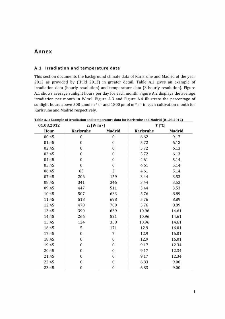
I
Annex
A.1 Irradiation and temperature data
This section documents the background climate data of Karlsruhe and Madrid of the year 2012 as provided by (Huld 2013) in greater detail. Table A.1 gives an example of irradiation data (hourly resolution) and temperature data (3-hourly resolution). Figure A.1 shows average sunlight hours per day for each month. Figure A.2 displays the average irradiation per month in W m-2. Figure A.3 and Figure A.4 illustrate the percentage of sunlight hours above 500 µmol m-2 s-1 and 1800 µmol m-2 s-1 in each cultivation month for Karlsruhe and Madrid respectively.
Table A.1: Example of irradiation and temperature data for Karlsruhe and Madrid (01.03.2012)
01.03.2012 I0 [W m-2] T [°C] Hour Karlsruhe Madrid Karlsruhe Madrid 00:45 0 0 6.62 9.17 01:45 0 0 5.72 6.13 02:45 0 0 5.72 6.13 03:45 0 0 5.72 6.13 04:45 0 0 4.61 5.14 05:45 0 0 4.61 5.14 06:45 65 2 4.61 5.14 07:45 206 159 3.44 3.53 08:45 341 346 3.44 3.53 09:45 447 511 3.44 3.53 10:45 507 633 5.76 8.89 11:45 518 698 5.76 8.89 12:45 478 700 5.76 8.89 13:45 390 639 10.96 14.61 14:45 266 521 10.96 14.61 15:45 124 358 10.96 14.61 16:45 5 171 12.9 16.01 17:45 0 7 12.9 16.01 18:45 0 0 12.9 16.01 19:45 0 0 9.17 12.34 20:45 0 0 9.17 12.34 21:45 0 0 9.17 12.34 22:45 0 0 6.83 9.00 23:45 0 0 6.83 9.00
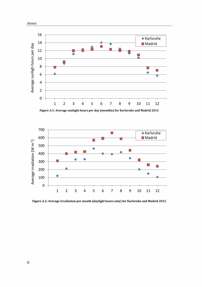
Annex
II
Figure A.1: Average sunlight hours per day (monthly) for Karlsruhe and Madrid 2012
Figure A.2: Average irradiation per month (daylight hours only) for Karlsruhe and Madrid 2012
0
2
4
6
8
10
12
14
16
0 1 2 3 4 5 6 7 8 9 10 11 12 13
Aver
age
sunl
igh
hour
s per
day
KarlsruheMadrid
0
100
200
300
400
500
600
700
0 1 2 3 4 5 6 7 8 9 10 11 12 13
Aver
age
irrad
iatio
n [W
m-2
]
KarlsruheMadrid
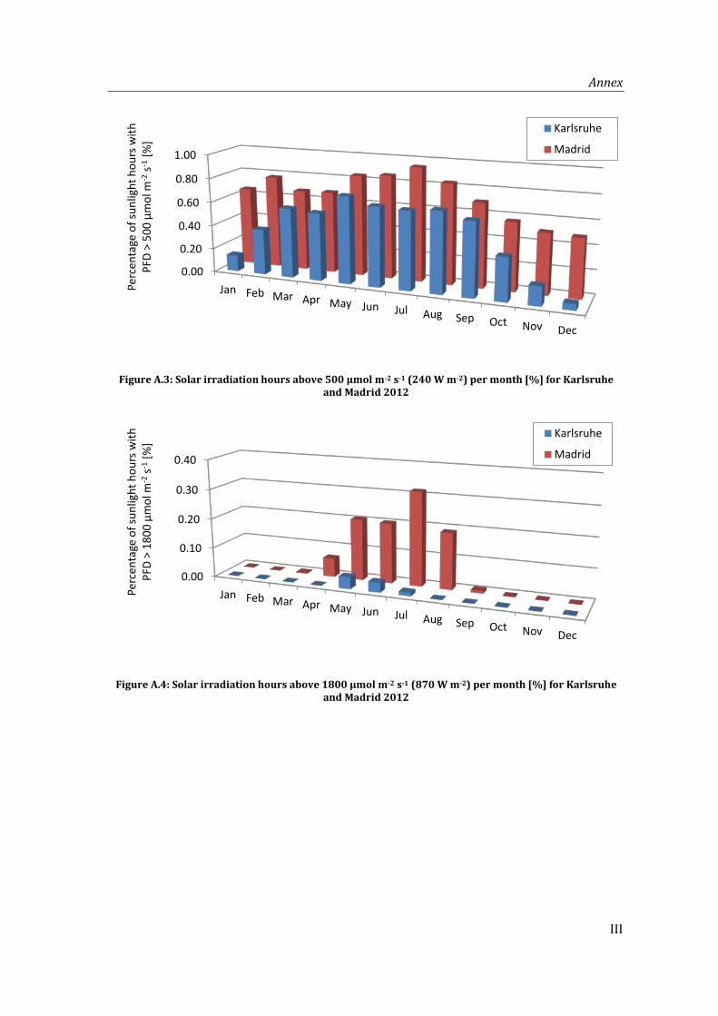
Annex
III
Figure A.3: Solar irradiation hours above 500 µmol m-2 s-1 (240 W m-2) per month [%] for Karlsruhe
and Madrid 2012
Figure A.4: Solar irradiation hours above 1800 µmol m-2 s-1 (870 W m-2) per month [%] for Karlsruhe
and Madrid 2012
0.00
0.20
0.40
0.60
0.80
1.00
Jan Feb Mar Apr May Jun Jul Aug Sep Oct Nov Dec
Perc
enta
ge o
f sun
light
hou
rs w
ith
PFD
> 50
0 µm
ol m
-2s-1
[%]
Karlsruhe
Madrid
0.00
0.10
0.20
0.30
0.40
Jan Feb Mar Apr May Jun Jul Aug Sep Oct Nov Dec
Perc
enta
ge o
f sun
light
hou
rs w
ith
PFD
> 18
00 µ
mol
m-2
s-1[%
]
Karlsruhe
Madrid
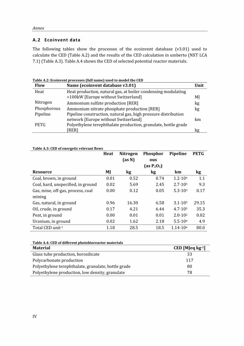
Annex
IV
A.2 Ecoinvent data
The following tables show the processes of the ecoinvent database (v3.01) used to calculate the CED (Table A.2) and the results of the CED calculation in umberto (NXT LCA 7.1) (Table A.3). Table A.4 shows the CED of selected potential reactor materials.
Table A.2: Ecoinvent processes (full name) used to model the CED Flow Name (ecoinvent database v3.01) Unit Heat Heat production, natural gas, at boiler condensing modulating
>100kW [Europe without Switzerland] MJ Nitrogen Ammonium sulfate production [RER] kg Phosphorous Ammonium nitrate phosphate production [RER] kg Pipeline Pipeline construction, natural gas, high pressure distribution
network [Europe without Switzerland] km PETG Polyethylene terephthalate production, granulate, bottle grade
[RER] kg
Table A.3: CED of energetic relevant flows Heat Nitrogen
(as N) Phosphor
ous (as P2O5)
Pipeline PETG
Resource MJ kg kg km kg Coal, brown, in ground 0.01 0.52 0.74 1.2⋅104 1.1 Coal, hard, unspecified, in ground 0.02 5.69 2.45 2.7⋅105 9.3 Gas, mine, off-gas, process, coal mining
0.00 0.12 0.05 5.3⋅103 0.17
Gas, natural, in ground 0.96 16.30 6.58 3.1⋅105 29.15 Oil, crude, in ground 0.17 4.21 6.44 4.7⋅105 35.3 Peat, in ground 0.00 0.01 0.01 2.0⋅102 0.02 Uranium, in ground 0.02 1.62 2.18 5.5⋅104 4.9 Total CED unit-1 1.18 28.5 18.5 1.14⋅106 80.0
Table A.4: CED of different photobioreactor materials Material CED [MJeq kg-1] Glass tube production, borosilicate 33 Polycarbonate production 117 Polyethylene terephthalate, granulate, bottle grade 80 Polyethylene production, low density, granulate 78
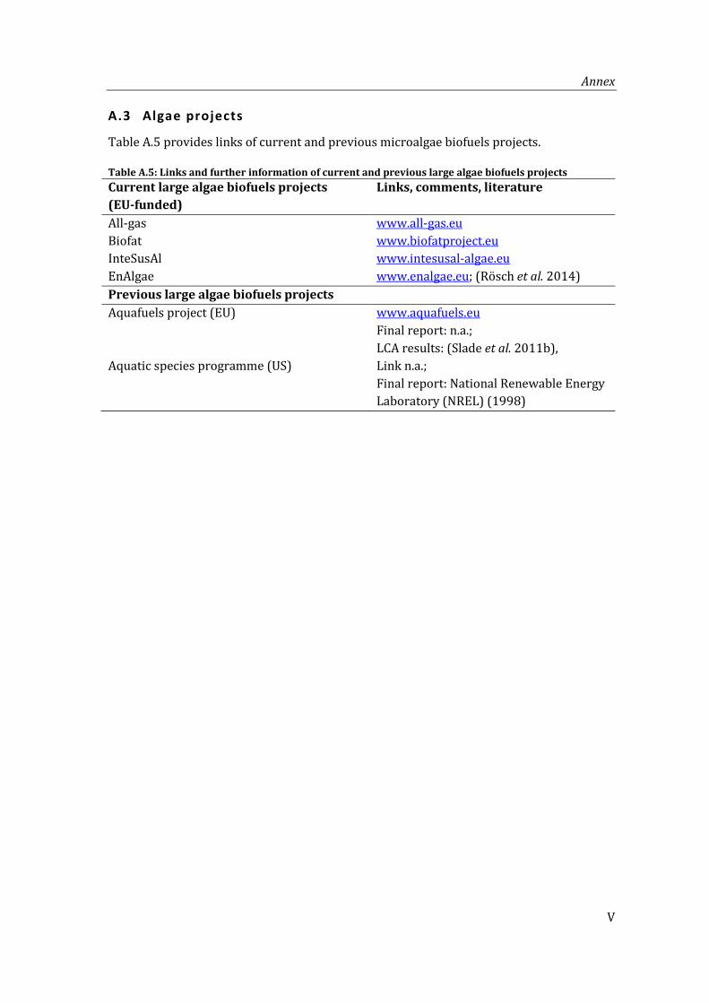
Annex
V
A.3 Algae projects
Table A.5 provides links of current and previous microalgae biofuels projects.
Table A.5: Links and further information of current and previous large algae biofuels projects Current large algae biofuels projects (EU-funded)
Links, comments, literature
All-gas www.all-gas.eu Biofat www.biofatproject.eu InteSusAl www.intesusal-algae.eu EnAlgae www.enalgae.eu; (Rösch et al. 2014) Previous large algae biofuels projects Aquafuels project (EU) www.aquafuels.eu
Final report: n.a.; LCA results: (Slade et al. 2011b),
Aquatic species programme (US) Link n.a.; Final report: National Renewable Energy Laboratory (NREL) (1998)
VI
References
Acién Fernández FG, Fernández Sevilla JM, Molina Grima E (2013): Photobioreactors for
the production of microalgae. Rev Environ Sci Biotechnol; 12 (2): 131–51.
Agrawal SC, Singh V (2000): Vegetative survival, akinete formation and germination in three blue-green algae and one green alga in relation to light intensity, temperature, heat shock and UV exposure. Folia Microbiol; 45 (5): 439–46.
Aitken D, Antizar-Ladislao B (2012): Achieving a green solution: limitations and focus points for sustainable algal fuels. Energies; 5 (12): 1613–47.
Althaus HJ, Chudacoff M, Hischier R, Jungbluth N, Osses M, Primas A (2007): Life Cycle Inventories of Chemicals; ecoinvent report No. 8, Dübendorf, CH.
Batan L, Quinn J, Willson B, Bradley T (2010): Net Energy and Greenhouse Gas Emission Evaluation of Biodiesel Derived from Microalgae. Environ. Sci. Technol; 44 (20): 7975–80.
Bilanovic D, Shelef G, Sukenik A (1988): Flocculation of microalgae with cationic polymers – Effects of medium salinity. Biomass; 17 (1): 65–76.
Bolton JR, Hall DO (1991): The maximum efficiency of photosynthesis. Photochemistry and Photobiology; 53 (4): 545–8.
Borowitzka MA (2013): Energy from microalgae: a short history. In: Borowitzka MA, Moheimani NR (eds.). Algae for biofuels and energy, Springer. Dordrecht, New York, p. 1-15.
Brentner LB, Eckelman MJ, Zimmerman JB (2011): Combinatorial life cycle assessment to inform process design of industrial production of algal biodiesel. Environ Sci Technol; 45 (16): 7060–7.
Burgess G, Fernández-Velasco JG (2007): Materials, operational energy inputs, and net energy ratio for photobiological hydrogen production. Int J Hydrogen Energy; 32 (9): 1225–34.
Burlew JS (1953): Current status of the large-scale culture of algae. In: Burlew JS (ed.). Algal culture: From laboratory to pilot plant, Carnegie Institution. Washington, DC.
Campbell PK, Beer T, Batten D (2011): Life cycle assessment of biodiesel production from microalgae in ponds. Special Issue: Biofuels - II: Algal Biofuels and Microbial Fuel Cells; 102 (1): 50–6.
Carvalho AP, Malcata FX (2001): Transfer of carbon dioxide within cultures of microalgae: plain bubbling versus hollow-fiber modules. Biotechnol Progr; 17 (2): 265–72.
References
VII
Carvalho AP, Meireles LA, Malcata FX (2006): Microalgal reactors: a review of enclosed system designs and performances. Biotechnol Progr; 22 (6): 1490–506.
Cheng-Wu Z, Zmora O, Kopel R, Richmond A (2001): An industrial-size flat plate glass reactor for mass production of Nannochloropsis sp. (Eustigmatophyceae). Aquaculture; 195 (1–2): 35–49.
Chiaramonti D, Prussi M, Casini D, Tredici MR, Rodolfi L, Bassi N et al. (2013): Review of energy balance in raceway ponds for microalgae cultivation: re-thinking a traditional system is possible; Special issue on advances in sustainable biofuel production and use - XIX International Symposium on Alcohol Fuels - ISAF. Appl Energy; 102: 101–11.
Chowdhury R, Viamajala S, Gerlach R (2012): Reduction of environmental and energy footprint of microalgal biodiesel production through material and energy integration. Bioresour Technol; 108: 102–11.
Clarens AF, Nassau H, Resurreccion EP, White MA, Colosi LM (2011): Environmental impacts of algae-derived biodiesel and bioelectricity for transportation; Environ Sci Technol; 45 (17): 7554–60.
Collet P, Hélias A, Lardon L, Ras M, Goy R, Steyer J (2011): Life-cycle assessment of microalgae culture coupled to biogas production. Special Issue: Biofuels - II: Algal Biofuels and Microbial Fuel Cells; 102 (1): 207–14.
Collet P, Spinelli D, Lardon L, Hélias A, Steyer J, Bernard O (2013): Life Cycle Assessment of microalgal-based biofuels. In: Pandey A, Lee D, Chisti, Yusuf, Soccol, Carlos Ricardo (eds.). Biofuels from algae, Elsevier, p. 287–312.
Dassey AJ, Hall SG, Theegala CS (2014): An analysis of energy consumption for algal biodiesel production: Comparing the literature with current estimates. Algal Research; 4: 89–95.
Deublein D, Steinhauser A (2011): Biogas from waste and renewable resources: An introduction. 2nd ed., Wiley-VCH, Weinheim.
Dillschneider R, Steinweg C, Rosello-Sastre R, Posten C (2013): Biofuels from microalgae: Photoconversion efficiency during lipid accumulation. Bioresour Technol; 142: 647–54.
DIN Deutsches Institut für Normung e.V. (2006): Environmental management - Life cycle assessment - Principles and framework (DIN EN ISO 14040), Beuth Verlag, Berlin.
DIN Deutsches Institut für Normung e.V. (2006): Environmental management - Life cycle assessment - Requirements and guidelines (DIN EN ISO 14044), Beuth Verlag, Berlin.
Doucha J, Straka F, Lívanský K (2005): Utilization of flue gas for cultivation of microalgae Chlorella sp. in an outdoor open thin-layer photobioreactor. J Appl Phycol; 17 (5): 403–12.
References
VIII
European Commission (2009): Commission regulation (EC) No 641/2009 implementing Directive 2005/32/EC of the European Parliament and of the Council with regard to ecodesign requirements for glandless standalone circulators and glandless circulators integrated in products.
European Parliament, European Council (2009): Directive 2009/28/EC of the European Parliament and of the Council of 23 April 2009 on the promotion of the use of energy from renewable sources and amending and subsequently repealing Directives 2001/77/EC and 2003/30/EC (Directive 2009/28/EC OJ 2009 L 140).
Fortier MP, Sturm BSM (2012): Geographic analysis of the feasibility of collocating algal biomass production with wastewater treatment plants. Environ Sci Technol; 46 (20): 11426–34.
Frank E, Elgowainy A, Han J, Wang Z (2013): Life cycle comparison of hydrothermal liquefaction and lipid extraction pathways to renewable diesel from algae. Mitig Adapt Strateg Glob Change; 18 (1): 137-158.
Franz A, Lehr F, Posten C, Schaub G (2012): Modeling microalgae cultivation productivities in different geographic locations - estimation method for idealized photobioreactors. Biotechnol J; 7 (4): 546–57.
Frischknecht R, Heijungs R, Hofstetter P (1998): Einstein’s lessons for energy accounting in LCA. Int. J. LCA; 3 (5): 266–72.
Geider RJ, Osborne BA (1989): Respiration and Microalgal Growth: A Review of the Quantitative Relationship between Dark Respiration and Growth. New Phytologist; 112 (3): 327–41.
Goldman JC (1979): Outdoor algal mass cultures – II. Photosynthetic yield limitations. Water Research; 13 (2): 119–36.
Golueke CG, Oswald WJ (1959): Biological Conversion of light energy to the chemical energy of methane. Applied microbiology; 7 (4): 219–27.
Grobbelaar J (1994): Turbulence in mass algal cultures and the role of light/dark fluctuations. J Appl Phycol; 6 (3): 331–5.
Grobbelaar JU (2003): Algal Nutrition ‒ Mineral Nutrition. In: Richmond A (ed.). Handbook of Microalgal Culture: Biotechnology and applied phycology, Blackwell Publishing Ltd. Oxford, UK, p. 95–115.
Gudin C, Chaumont D (1991): Cell fragility – The key problem of microalgae mass production in closed photobioreactors. Algal biotechnology; 38 (2–3): 145–51.
Günther A, Jakob T, Goss R, König S, Spindler D, Räbiger N et al. (2012): Methane production from glycolate excreting algae as a new concept in the production of biofuels. Bioresour Technol; 121: 454–7.
Gürzenich D, Mathur J, Bansal N, Wagner H (1999): Cumulative energy demand for selected renewable energy technologies. Int. J. LCA; 4 (3): 143-149.
References
IX
Hall CAS, Balogh S, Murphy DJ (2009): What is the Minimum EROI that a Sustainable Society Must Have? Energies; 2 (1): 25–47.
Hallenbeck PC, Benemann JR (2002): Biological hydrogen production; fundamentals and limiting processes. Int J Hydrogen Energy; 27 (11-12): 1185–93.
Harris DO (1970): Growth inhibitors produced by the green algae (Volvocaceae). Archiv. Mikrobiol; 76 (1): 47-50.
Heijungs R, Huijbregts MAJ (2004): A review of approaches to treat uncertainty in LCA; Available from: http://www.iemss.org/iemss2004/pdf/lca/heijarev.pdf. [November 22, 2015].
Hirschberg HG (1999): Handbuch der Verfahrenstechnik und Anlagenbau; Chemie, Technik, Wirtschaftlichkeit ; mit 689 Tabellen, Springer, Berlin [u.a.].
Hischier R, Weidema B (2009): Implementation of Life Cycle Impact Assessment Methods; ecoinvent report No. 3, v2.1, Dübendorf, CH.
Hu Q, Guterman H, Richmond A (1996): A flat inclined modular photobioreactor for outdoor mass cultivation of photoautotrophs. Biotechnol Bioeng; 51 (1): 51–60.
Hu Q, Richmond A (1996): Productivity and photosynthetic efficiency of Spirulina platensis as affected by light intensity, algal density and rate of mixing in a flat plate photobioreactor. J Appl Phycol; 8 (2): 139–45.
Hu Q, Zarmi Y, Richmond A (1998): Combined effects of light intensity, light-path and culture density on output rate of Spirulina platensis (Cyanobacteria). European Journal of Phycology; 33 (2): 165–71.
Hulatt CJ, Thomas DN (2011): Energy efficiency of an outdoor microalgal photobioreactor sited at mid-temperate latitude. Bioresour Technol; 102 (12): 6687–95.
Huld T (2013): Irradiation and temperature data Karlsruhe and Madrid 2012. E-mail, 16.12.2013, Ispra, Italy.
Huld T, Müller R, Gambardella A (2012): A new solar radiation database for estimating PV performance in Europe and Africa. Solar Energy; 86 (6): 1803–15.
Jacobi A, Bucharsky EC, Schell KG (2012): The application of transparent glass sponge for improvement of light distribution in photobioreactors. J Bioproces Biotechniq; 02 (01).
Jacovides CP, Timvios FS, Papaioannou G, Asimakopoulos DN, Theofilou CM (2004): Ratio of PAR to broadband solar radiation measured in Cyprus. Agricultural and Forest Meteorology; 121 (3–4): 135–40.
Janssen M, Tramper J, Mur LR, Wijffels RH (2003): Enclosed outdoor photobioreactors: Light regime, photosynthetic efficiency, scale-up, and future prospects. Biotechnol Bioeng; 81 (2): 193–210.
References
X
Jonker JGG, Faaij APC (2013): Techno-economic assessment of micro-algae as feedstock for renewable bio-energy production; Special Issue on Advances in sustainable biofuel production and use - XIX International Symposium on Alcohol Fuels - ISAF. Appl Energy; 102: 461–75.
Jorquera O, Kiperstok A, Sales EA, Embiruçu M, Ghirardi ML (2010): Comparative energy life-cycle analyses of microalgal biomass production in open ponds and photobioreactors. Bioresour Technol; 101 (4): 1406–13.
Jungbluth N, Chudacoff M, Dauriat A, Dinkel F, Doka M, Faist-Emmenegger M et al. (2007): Life Cycle Inventories of Bioenergy; ecoinvent report No. 17, Dübendorf, CH.
Kadam KL (2002): Environmental implications of power generation via coal-microalgae cofiring. Energy; 27 (10): 905–22.
Kalweit A, Paul C, Peters S, Wallbaum R (eds.) (2012): Handbuch für Technisches Produktdesign; Material und Fertigung, Entscheidungsgrundlagen für Designer und Ingenieure, Springer, Berlin.
Kamen MD (1963): Primary processes in photosynthesis, Academic Press, New York.
Khoo HH, Sharratt PN, Das P, Balasubramanian RK, Naraharisetti PK, Shaik S (2011): Life cycle energy and CO2 analysis of microalgae-to-biodiesel: Preliminary results and comparisons. Bioresour Technol; 102 (10): 5800–7.
Kliphuis AMJ, Winter L de, Vejrazka C, Martens DE, Janssen M, Wijffels RH (2010): Photosynthetic efficiency of Chlorella sorokiniana in a turbulently mixed short light-path photobioreactor. Biotechnol Progr; 26 (3): 687–96.
Klöpffer W, Grahl B (2009): Ökobilanz (LCA); Ein Leitfaden für Ausbildung und Beruf, Wiley-VCH, Weinheim.
Kok B (1953): Experiments on photosynthesis by Chlorella in flashing light. In: Burlew JS (ed.). Algal culture: From laboratory to pilot plant, Carnegie Institution. Washington, DC, p. 63–75.
Lardon L, Helias A, Sialve B, Steyer JP, Bernard O (2009): Life-Cycle Assessment of Biodiesel Production from Microalgae. Environ Sci Technol; 43 (17): 6475–81.
Lehr F (2012): Wasserstoff-Erzeugung mit Mikroalgen; Prozessintensivierung durch integrierte Verfahrensetnwicklung. Dissertation, Karlsruhe.
Lehr F, Posten C (2009): Closed photo-bioreactors as tools for biofuel production. Curr Opin Biotech; 20 (3): 280–5.
Lundquist TJ, Woertz IC, Quinn NWT, Benemann JR (2010): A realistic technology and engineering assessment of algae biofuel production.
Madigan MT, Martinko JM, Brock TD (2006): Brock Biology of microorganisms. 11th ed., Pearson/Prentice Hall, Upper Saddle River, N.J.
References
XI
Meyer M (2012): Economic anlysis of energy and matter generation from microalgae; An environmental LCC model for hydrogen and biogas prodcution from Chlamydomonas reinhardtii. Masterarbeit, Uppsala; Available from: http://stud.epsilon.slu.se. [November 22, 2015].
Meyer MA, Weiss A (2014): Life cycle costs for the optimized production of hydrogen and biogas from microalgae. Energy; 78: 84–93.
Morweiser M, Kruse O, Hankamer B, Posten C (2010): Developments and perspectives of photobioreactors for biofuel production. Appl Microbiol Biotechnol; 87 (4): 1291–301.
Mu D, Min M, Krohn B, Mullins KA, Ruan R, Hill J (2014): Life cycle environmental impacts of wastewater-based algal biofuels. Environ Sci Technol; 48 (19): 11696–704.
Murphy CF, Allen DT (2011): Energy-water nexus for mass cultivation of algae. Environ Sci Technol; 45 (13): 5861–8.
Mussgnug JH, Klassen V, Schlüter A, Kruse O (2010): Microalgae as substrates for fermentative biogas production in a combined biorefinery concept. J Biotechnol; 150 (1): 51–6.
Mussgnug JH, Thomas-Hall S, Rupprecht J, Foo A, Klassen V, McDowall A et al. (2007): Engineering photosynthetic light capture: impacts on improved solar energy to biomass conversion. Plant Biotech J; 5 (6): 802–14.
National Renewable Energy Laboratory (NREL) (1998): A Look Back at the U.S. Department of Energy’s Aquatic Species Program: Biodiesel from Algae; Close out report. Prepared for the US Department of Energy (DOE), Golden, Colorado.
Nič M, Jirát J, Košata B, Jenkins A, McNaught A (eds.) (2009): IUPAC. Compendium of Chemical Terminology; the "Gold Book", 2nd ed., Blackwell Scientific Publications, Research Triagle Park, NC.
Norsker N, Barbosa MJ, Vermuë MH, Wijffels RH (2011): Microalgal production – A close look at the economics. Biotechnol Adv; 29 (1): 24–7.
OCAP (2012): OCAP Factsheet; CO2 v.o.f., Schiedam, NL; Available from: http://www.ocap.nl/files/Ocap_Factsheet2012_UK.pdf. [November 22, 2015].
Öschger L, Posten C (2012): Construction and assessment parameters of photobioreactors. In: Posten C, Walter C (eds.). Microalgal biotechnology: Potential and production, Walter de Gruyter. Berlin, Boston.
Patyk A, Reinhardt GA (1997): Düngemittel - Energie- und Stoffstrombilanzen, Vieweg, Braunschweig/Wiesbaden.
Perry MJ, Talbot MC, Alberte RS (1981): Photoadaption in marine phytoplankton: Response of the photosynthetic unit. Mar. Biol; 62 (2-3): 91–101.
Posten C (2009): Design principles of photo-bioreactors for cultivation of microalgae. Eng Life Sci; 9 (3): 165–77.
References
XII
Posten C, Walter C (eds.) (2012): Microalgal biotechnology; Integration and economy, Walter de Gruyter, Berlin, Boston.
Pruvost J (2011): Cultivation of algae in photobioreactors for biodiesel production. In: Pandey A, Larroche C, Ricke, S. C., Dussap, C. G., Gnansounou, E. (eds.). Biofuels: Alternative feedstocks and conversion processes, 1st ed., Academic Press. Amsterdam, Boston, p. 439–464.
Pulz O (2001): Photobioreactors: production systems for phototrophic microorganisms. Appl Microbiol Biotechnol; 57 (3): 287–93.
Quinn JC, Yates T, Douglas N, Weyer K, Butler J, Bradley TH et al. (2012): Nannochloropsis production metrics in a scalable outdoor photobioreactor for commercial applications. Bioresour Technol; 117: 164–71.
Rawat I, Ranjith Kumar R, Mutanda T, Bux F (2013): Biodiesel from microalgae: A critical evaluation from laboratory to large scale production. Appl Energy; 103: 444–67.
Razon LF, Tan RR (2011): Net energy analysis of the production of biodiesel and biogas from the microalgae: Haematococcus pluvialis and Nannochloropsis. Appl Energy; 88 (10): 3507–14.
Richards BS, Watt ME (2007): Permanently dispelling a myth of photovoltaics via the adoption of a new net energy indicator. Renew Sust Energ Rev; 11 (1): 162–72.
Richmond A, Cheng-Wu Z (2001): Optimization of a flat plate glass reactor for mass production of Nannochloropsis sp. outdoors. J Biotechnol; 85 (3): 259–69.
Ripplinger P (2008): Wertstoffe aus dem Flachplatten-Airlift-Reaktor; Subitec GmbH, Stuttgart., Präsentation Januar 2008, Stuttgart.
Rodolfi L, Chini Zittelli G, Bassi N, Padovani G, Biondi N, Bonini G et al. (2009): Microalgae for oil: Strain selection, induction of lipid synthesis and outdoor mass cultivation in a low-cost photobioreactor. Biotechnol Bioeng; 102 (1): 100–12.
Roels JA, Heijnen JJ (1980): Power dissipation and heat production in bubble columns: Approach based on nonequilibrium thermodynamics. Biotechnol. Bioeng; 22 (11): 2399–404.
Rösch C, Skarka J, Wegerer N (2012): Materials flow modeling of nutrient recycling in biodiesel production from microalgae. Bioresour Technol; 107: 191–9.
Rösch C, Skarka J, Kugler F (2014): Results of the EnAlgae Stakeholder Workshop on "Benefits and Risks from Biomass Production with Microalgae"; Held at Frankfurt Airport, Germany On 5th June 2014; Available from: www.enalgae.eu/getfile.php?type=site_documents&id=WP2A11%20benefits%20stakeholder%20workshop%20report%205Jun14.pdf. [November 22, 2015].
Rosenblueth A, Wiener N (1945): The Role of Models in Science. Philosophy of Science; 12 (4): 316–21.
Sander K, Murthy GS (2010): Life cycle analysis of algae biodiesel. Int J LCA: 1–11.
References
XIII
Sawayama S, Minowa T, Yokoyama S (1999): Possibility of renewable energy production and CO2 mitigation by thermochemical liquefaction of microalgae. Biomass and Bioenergy; 17 (1): 33–9.
Sevigné Itoiz E, Fuentes-Grünewald C, Gasol CM, Garcés E, Alacid E, Rossi S et al. (2012): Energy balance and environmental impact analysis of marine microalgal biomass production for biodiesel generation in a photobioreactor pilot plant. Biorefinery; 39: 324–35.
Shirvani T, Yan X, Inderwildi OR, Edwards PP, King DA (2011): Life cycle energy and greenhouse gas analysis for algae-derived biodiesel. Energy Environ. Sci; 4 (10): 3773.
Sialve B, Bernet N, Bernard O (2009): Anaerobic digestion of microalgae as a necessary step to make microalgal biodiesel sustainable. Biotechnol Adv; 27 (4): 409–16.
Sierra E, Acién FG, Fernández JM, Garcí-a JL, González C, Molina E (2008): Characterization of a flat plate photobioreactor for the production of microalgae. Chem Eng J; 138 (1-3): 136–47.
Sills DL, Paramita V, Franke MJ, Johnson MC, Akabas TM, Greene CH et al. (2012): Quantitative uncertainty analysis of life cycle assessment for algal biofuel production. Environ Sci Technol; 47 (2): 687–94.
Skarka J (2015): Potenziale zur Erzeugung von Biomasse aus Mikroalgen in Europa unter besonderer Berücksichtigung der Flächen- und CO2-Verfügbarkeit. Dissertation, Karlsruhe; Available from: http://nbn-resolving.org/urn:nbn:de:swb:90-469308. [November 22, 2015].
Slade R, Xu D, Bauen A (2011a): The Sustainability of Algae Biofuels: LCA ,Environmental and Economic Impacts; AquaFUELs project, final conference (30.06.2011); Available from: http://www.aquafuels.eu/attachments/076_08%20-%20R.Slade%20-%20LCA,%20environmental%20&%20economic%20assessment.pdf. [November 22, 2015].
Slade R, Xu D, Bauen A (2011b): Life-cycle assessment and environmental assessment; Deliverables 3.3 and 3.5 of the proposal: Algae and aquatic biomass for a sustainable production of 2nd generation biofuels (AquaFUELs); Available from: http://www.aquafuels.eu/attachments/079_D%203.3-3.5%20Life-Cycle%20Assessment%20and%20Environmental%20Assessment.pdf. [November 22, 2015].
Slegers PM, Wijffels RH, van Straten G, van Boxtel AJB (2011): Design scenarios for flat panel photobioreactors; Special Issue of Energy from algae: Current status and future trends. Appl Energy; 88 (10): 3342–53.
SoDa: Solar radiation data; Available from: http://www.soda-is.com/eng/services/service_invoke/gui.php?xml_descript=hc1_month.xml#parameters. [September 30, 2014].
References
XIV
Sousa C, Winter L de, Janssen M, Vermuë MH, Wijffels RH (2012): Growth of the microalgae Neochloris oleoabundans at high partial oxygen pressures and sub-saturating light intensity. Bioresour Technol; 104: 565–70.
Stephenson AL, Kazamia E, Dennis JS, Howe CJ, Scott SA, Smith AG (2010): Life-Cycle Assessment of Potential Algal Biodiesel Production in the United Kingdom: A Comparison of Raceways and Air-Lift Tubular Bioreactors; Energy & Fuels. Energy Fuels; 24 (7): 4062–77.
Sukarni, Sudjito, Hamidi N, Yanuhar U, Wardana I (2014): Potential and properties of marine microalgae Nannochloropsis oculata as biomass fuel feedstock. International Journal of Energy and Environmental Engineering; 5 (4): 279–90.
Tamiya EL, Hase E, Shibata AM, Iwamura T, Nihei T, Saha T (1953): Kinetics of growth of Chlorella with special reference to its dependence on quantity of available light and on temperature. In: Burlew JS (ed.). Algal culture: From laboratory to pilot plant, Carnegie Institution. Washington, DC.
Torzillo G, Pushparaj B, Bocci F, Balloni W, Materassi R, Florenzano G (1986): Production of Spirulina biomass in closed photobioreactors. Biomass; 11 (1): 61–74.
Torzillo G, Sacchi A, Materassi R, Richmond A (1991): Effect of temperature on yield and night biomass loss in Spirulina platensis grown outdoors in tubular photobioreactors. J Appl Phycol; 3 (2): 103–9.
Tredici MR (2010): Photobiology of microalgae mass cultures: understanding the tools for the next green revolution. Biofuels; 1 (1): 143–62.
Tredici MR (2003): Mass Production of Microalgae: Photobioreactors. In: Richmond A (ed.). Handbook of Microalgal Culture: Biotechnology and applied phycology, Blackwell Publishing Ltd. Oxford, UK, p. 178–214.
Tredici MR, Bassi N, Prussi M, Biondi N, Rodolfi L, Chini Zittelli G et al. (2015): Energy balance of algal biomass production in a 1-ha “Green Wall Panel” plant: How to produce algal biomass in a closed reactor achieving a high Net Energy Ratio. Applied Energy; 154: 1103–11.
Tredici MR, Materassi R (1992): From open ponds to vertical alveolar panels: the Italian experience in the development of reactors for the mass cultivation of phototrophic microorganisms. J Appl Phycol; 4 (3): 221-231.
Ugwu CU, Aoyagi H, Uchiyama H (2008): Photobioreactors for mass cultivation of algae. Bioresour Technol; 99 (10): 4021–8.
Umweltbundesamt (2014): Entwicklung des Brennstoffnutzungsgrades fossiler Kraftwerke; Available from: http://www.umweltbundesamt.de/daten/energiebereitstellung-verbrauch/stromerzeugung#textpart-5. [November 22, 2015].
Vasudevan V, Stratton RW, Pearlson MN, Jersey GR, Beyene AG, Weissman JC et al. (2012): Environmental performance of algal biofuel technology options; Environ Sci Technol; 46 (4): 2451–9.
References
XV
Verein deutscher Ingenieure (VDI) (2012): Cumulative energy demand (CED), Terms, definitions, methods of calculation; ICS 01.040.27, 27.100 (VDI 4600), Beuth Verlag, Berlin.
Walker DA (1992): Tansley Review No. 36 Excited leaves. New Phytologist; 121 (3): 325–45.
Walker DA (2009): Biofuels, facts, fantasy, and feasibility. J Appl Phycol; 21 (5): 509–17.
Walker DA (2010): Biofuels – for better or worse? Annals of Applied Biology; 156 (3): 319–27.
Waltz E (2009): Biotech's green gold? Nat Biotechnol; 27 (1): 15–8.
Weinberg J, Kaltschmitt M, Wilhelm C (2012): Analysis of greenhouse gas emissions from microalgae-based biofuels. Biomass Conv Bioref; 2 (2): 179–94.
Weissman JC, Goebel RP, Benemann JR (1988): Photobioreactor design: mixing, carbon utilization, and oxygen accumulation. Biotechnology and bioengineering; 31 (4): 336–44.
Wijffels RH, Barbosa MJ (2010): An outlook on microalgal biofuels. Science; 329 (5993): 796–9.
Wilhelm C, Jakob T (2011): From photons to biomass and biofuels: evaluation of different strategies for the improvement of algal biotechnology based on comparative energy balances. Appl Microbiol Biotechnol; 92 (5): 909–19.
Wilhelm C, Jakob T (2012): Balancing the conversion efficiency from photon to biomass. In: Posten C, Walter C (eds.). Microalgal biotechnology: Potential and production, Walter de Gruyter. Berlin, Boston.
Wilhelm C, Selmar D (2011): Energy dissipation is an essential mechanism to sustain the viability of plants: The physiological limits of improved photosynthesis. J Plant Physiol; 168 (2): 79–87.
Williams P, Thomas DN, Reynolds CS (2008): Phytoplankton Productivity: Carbon Assimilation in Marine and Freshwater Ecosystems, Wiley.
Williams PJ, Laurens LM (2010): Microalgae as biodiesel & biomass feedstocks: Review & analysis of the biochemistry, energetics & economics. Energy Environ Sci; 3 (5): 554–90.
Woertz IC, Benemann JR, Du N, Unnasch S, Mendola D, Mitchell, B. Greg et al. (2014): Life cycle GHG emissions from microalgal biodiesel – A CA-GREET Model. Environ. Sci. Technol; 48 (11): 6060–8.
Wykoff DD, Davies JP, Melis A, Grossman AR (1998): The regulation of photosynthetic electron transport during nutrient deprivation in Chlamydomonas reinhardtii. Plant Physiol; 117 (1): 129–39.

References
XVI
Zamalloa C, Vulsteke E, Albrecht J, Verstraete W (2011): The techno-economic potential of renewable energy through the anaerobic digestion of microalgae. Bioresour Technol; 102 (2): 1149–58.
Zhu X, Long SP, Ort D (2008): What is the maximum efficiency with which photosynthesis can convert solar energy into biomass? Curr Opin Biotech; 19 (2): 153–9.

XVII
Acknowledgements
I would like to thank my advisor Prof. Liselotte Schebek (TU Darmstadt) and my supervisor Dr. Andreas Patyk (ITAS), who made this work possible. I also thank my second advisor Prof. Peter Cornel (TU Darmstadt), for his helpful comments.
This dissertation was written at the Institute for Technology Assessment and Systems Analysis (ITAS) at the Karlsruhe Institute of Technology. I thank my colleagues at ITAS for their support and inspiring discussions, especially the Simulanten group.
Many thanks go to Thomas Huld (Joint Research Centre) for providing the temperature and irradiation data.
I am very grateful to Oliver, Magdalena, Kirsten, Bernardo, Sonja and Dominik for helping me in various ways, be it by reading the manuscript, by encouraging me in difficult times, or by practical help with debugging the model.
Special thanks go to Andi and my family for their love and support.
Academic career of Annika Weiss
since 2010 Researcher at the Karlsruhe Institute of Technology (KIT), Institute for Technology Assessment and Systems Analysis (ITAS), Karlsruhe
2010 - 2015 Dissertation ‘Energy balance of microalgae biofuels’ at the IWAR Institute, Technical University of Darmstadt
2009 Researcher at the University of Manchester, School of Earth, Atmospheric, and Environmental Sciences, Manchester, UK
2002 – 2009
2008
2006/07
Studies of Environmental Engineering (Dipl.-Ing.), major subjects: water treatment and environmental biotechnology at the Technical University of Berlin (Diplom) and University of Stuttgart (Vordiplom) Diploma thesis ‘Development of a biological treatment process for dye wastewater’ in Manchester, UK Undergraduate thesis ‘Antibiotic resistant bacteria in extreme environments of Andean wetlands’ at the industrial microbiology pilot plant PROIMI in Tucuman, Argentina

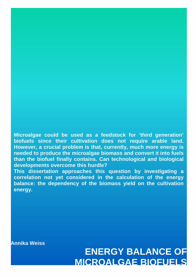
Annika Weiss
ENERGY BALANCE OF MICROALGAE BIOFUELS
Microalgae could be used as a feedstock for ‘third generation’ biofuels since their cultivation does not require arable land. However, a crucial problem is that, currently, much more energy is needed to produce the microalgae biomass and convert it into fuels than the biofuel finally contains. Can technological and biological developments overcome this hurdle? This dissertation approaches this question by investigating a correlation not yet considered in the calculation of the energy balance: the dependency of the biomass yield on the cultivation energy.


![Edld 5352 week01_assignmentjbuckels_ea1189[1]](https://img.dokumen.tips/doc/110x75/548f3c36b4795991608b4791/edld-5352-week01assignmentjbuckelsea11891.jpg)
![[5352]-503 CEGP013091](https://img.dokumen.tips/doc/110x75/61fa19cdf313ba794c314e19/5352-503-cegp013091.jpg)

![Edld 5352 week04_assignment[1]](https://img.dokumen.tips/doc/110x75/54b4568c4a79591c698b46f7/edld-5352-week04assignment1-5584a7bdceb96.jpg)