Embed Size (px)
Citation preview

International Journal of Applied Engineering and Technology ISSN: 2277-212X (Online)
An Online International Journal Available at http://www.cibtech.org/jet.htm
2012 Vol. 2 (2) April-June, pp.101-139/Singh
Research Article
101
ENDOSCOPIC OPTICAL COHERENCE TOMOGRAPHY *Akash K Singh
IBM Corporation Sacramento USA
*Author for Correspondence
ABSTRACT
Real-time in-vivo forward-viewing optical coherence tomography imaging has been demonstrated with a
novel lens scanning based MEMS endoscope catheter. An endoscopic catheter with an outer dimension of
7 mm x 7 mm has been designed, manufactured and assembled. By employing high-speed spectral
domain optical coherence tomography, in-vivo two-dimensional cross-sectional images of human skin
tissues were obtained as a preliminary study. Imaging speed of 122 frames per second and axial resolution
of 7.7 μm is accomplished. The operation voltages are only DC 3 V and AC 6 Vpp at resonance
frequency of 122 Hz. The catheter can provide many opportunities for clinical applications such as
compact packaging, long working distance and body safe low operating voltages.
Key Words: Lens Scanner, Optical Coherence Tomography (Oct), Spectral Domain Optical Coherence
Tomography (Sd-Oct), Endoscopic Catheter, Micro-Optical Bench
INTRODUCTION
Optical coherence tomography (OCT) has been demonstrated as a high emerging optical imaging
modality, particularly in acquiring in-vivo real-time cross-sectional information of high scattering media
with micrometerscale spatial resolution Huang et al., (1991). Moreover, high-speed, noninvasive, and
non-contact imaging capability of Fourier domain optical coherence tomography has enhanced the growth
of various endoscopic OCT. Their beam scanning mechanisms are mainly categorized as follows: rotating
a fiber-prism assembly at the proximal end, microelectromechanical system (MEMS) mirror, a resonant
cantilever fiber driven by piezoelectric tube, and others. The fiberprism method is suitable for
circumferential imaging but limited by motion-induced artifacts as a result of slow scan speed Tearney et
al., (1997). MEMS mirror based endoscopic probes are separated into three kinds: electrostatic Jung et al.,
(2006), electro-thermal Pan et al., (2001) and Sun et al., (2010) and electromagnetic actuators Kim et al.,
(2007). They could achieve high-speed side-view imaging, despite relatively large device footprints and
high actuation voltages. A fiber cantilever probe is a forward endoscopic imaging embodiment. However,
it has a low coupling efficiency in large-scan angles Liu et al., (2004) and Huo et al., (2010) and Wu et
al., (2009). The previous works have still technical challenges in minimal endoscopic packaging and low
operating voltages with high signal-to-noise ratio. This work presents a fully packaged endoscopic
catheter using the lens scanning module. Recently, we have reported two dimensional lens microstages as
a forward optical scanning module Park et al., (2010). The scanning module is composed by a pigtailed
gradient index (GRIN) lens fiber collimator (GRINTECH GmbH, lens diameter: 1.6 mm, clear aperture:
0.53 mm), two commercialized high quality aspheric glass lenses (ALPS Electric Co., LTD., lens
diameter: 1 mm, f = 0.5 mm, clear aperture: 0.6 mm) and two electrostatic MEMS actuators to move two
lenses perpendicular axis. Two electrostatic MEMS actuators are integrated on a monolithically fabricated
silicon micro optical bench with fiber groove and lens holder structures. The fiber groove and lens holder
structures are designed to assist precise optical alignment during the assembly. Thus, it helps to minimize
the off-axis aberrations that are induced by beam scanning. Experiment show a scanning electron
microscope image of fabricated micro optical bench and a perspective view of the lens scanning module
assembled on an endoscope catheter. It is clearly shown that all optical components are precisely aligned
along the optical axis on top of the silicon micro optical bench. The proposed lens scanning based
endoscopic catheter provides three main advantages for real clinical applications: First, the forward
viewing and pre-objective scanning is desirable for clinical usage, since it can easily locate the probe on a
target area of interest and examine suspicious tissues with long working distance. Second, the lens
International Journal of Applied Engineering and Technology ISSN: 2277-212X (Online)
An Online International Journal Available at http://www.cibtech.org/jet.htm
2012 Vol. 2 (2) April-June, pp.101-139/Singh
Research Article
102
scanning module with high Q-factor provides body-safe low voltage operation. Finally, the high fill-factor
of the lens scanning module secures the compactness of the endoscopic catheter by vertically mounting
all optical components on silicon micro optical bench without the reduction of clear aperture
Endoscopedoscope Catheter
The endoscope catheter, including the lens scanning module, is made of aluminum housing and the outer
size is 7 mm x 7 mm with objective lens diameter of 5 mm. Experiment shows optical image of the lens
scanning based endoscopic MEMS catheter. The sharp edges of the aluminum housing were smoothed
and the entire assembly was leak-free packaged to protect a patient from electrical shocks or any
scratches. The objective mount head was designed to change an objective lens according to various
applications. For the assembly process, the optical axis was firstly set by using a fiber collimator and an
objective lens. To prevent optical aberrations due to machining tolerance of the aluminum housing, the
gradient index (GRIN) lens fiber collimator and the objective lens were carefully positioned by
monitoring the beam shape at the image plane. Secondly, the MEMS scanner module was aligned along
the optical axis using the fiber groove. The fiber groove helps to avoid rotational errors, since the fiber
collimator restricts the rotation of the device. Finally, two scanning lenses are laterally integrated on top
of the silicon lens holders with MEMS scanners, which are designed to put the lenses into it. The size of
the lens holders are designed to grab the lenses tightly. Therefore, once a MEMS scanner aligned to the
optical axis, the scanning lenses can be aligned to the optical axis intrinsically.
Spectral Domain Optical Coherence Tomography System
In this work, high-speed spectral domain optical coherence tomography (SD-OCT) is employed for
forward viewing endoscopic OCT catheter. Experimenture 3 describes the experimental set-up of SD-
OCT combined with the MEMS endoscopic catheter. The SD-OCT system consists of a broadband
superluminescent light emitting diode (Exalos, λ0 = 830.9 nm, Δλ = 46.8 nm, Max. Power = 4.99 mW ), a
2 x 2 coupler, and a home-built spectrometer composed of a volume phase holographic grating (Wasatch
Photonics, VPHG, 1200 lpmm), a near-infrared (NIR) achromatic camera lens (Thorlab, f = 200 mm), a
CMOS line scan camera (Basler, spL 2048-70 km) with 2048 pixel elements, and a high-speed frame
grabber (National Instruments, PCIe-1429). The high-speed camera link type frame grabber can transfer
two-dimensional interference data (512 x 2048 pixels) into a hard disk at a rate of 122 frames per second.
One axial scan time corresponding to the camera exposure period is about 15 μsec. In-vivo real-time
cross-sectional imaging was realized with Labview from the measured two-dimensional interference
spectra. DC and autocorrelation noises included in each axial scan spectrum can deteriorate the quality of
the final image after Fourier transformation. Thus, the ensemble average of all axial scan spectra are
subtracted from each axial scan data before Fourier Transformation [11], with removal of fixed pattern
noises. The axial scan spectra acquired from the line CMOS camera are evenly sampled in the wavelength
domain, thus becoming evenly re-sampled by linear interpolation in the wavenumber domain [12]. The
broadband SLED laser beam has the theoretical axial resolution of 6.49 μm in air. To avoid a dispersion
mismatch between two arms, an identical GRIN lens collimator is implemented in both the sample arm
and the reference arm. The spectrometer resolution of 0.06 nm determines the maximum imaging depth
range of about 3 mm in air.
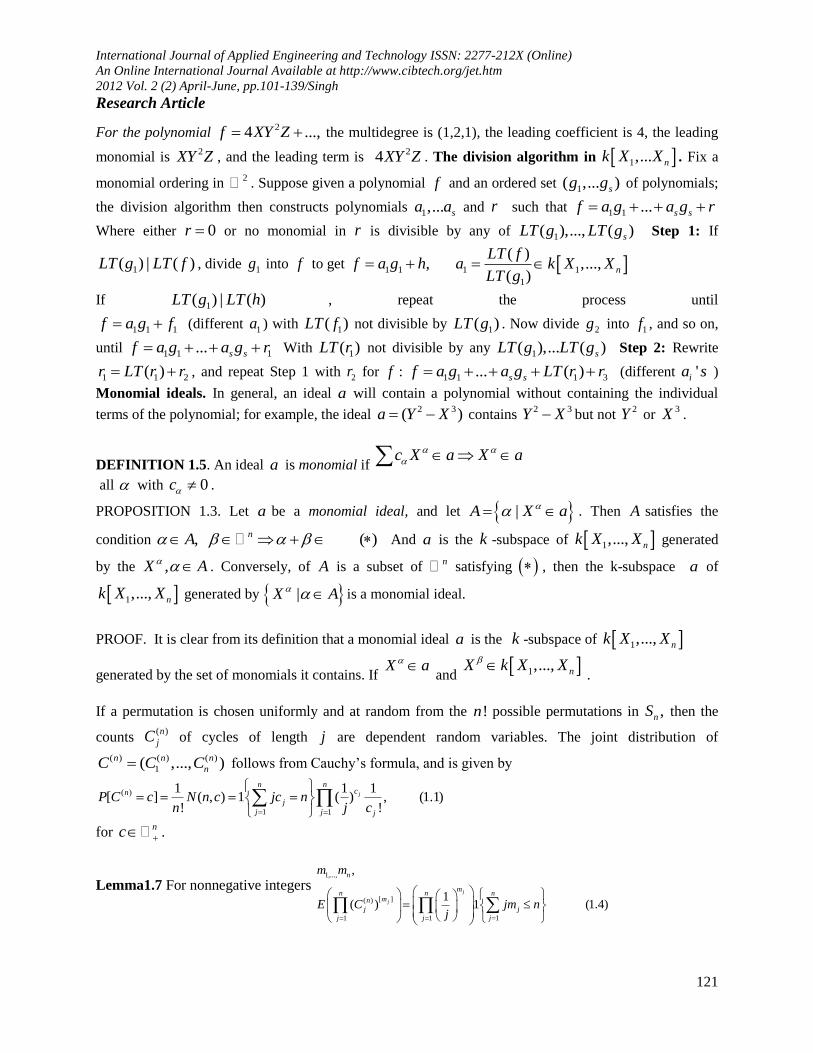
We consider the following anycast field equations defined over an open bounded piece of network and /or
feature spacedR . They describe the dynamics of the mean anycast of each of p node populations.
|
1
( ) ( , ) ( , ) [( ( ( , ), ) )]
(1)( , ), 0,1 ,
( , ) ( , ) [ ,0]
p
i i ij j ij j
j
ext
i
i i
dl V t r J r r S V t r r r h dr
dt
I r t t i p
V t r t r t T
International Journal of Applied Engineering and Technology ISSN: 2277-212X (Online)
An Online International Journal Available at http://www.cibtech.org/jet.htm
2012 Vol. 2 (2) April-June, pp.101-139/Singh
Research Article
103
We give an interpretation of the various parameters and functions that appear in (1), is finite piece of
nodes and/or feature space and is represented as an open bounded set of dR . The vector r and r
represent points in . The function : (0,1)S R is the normalized sigmoid function:
1
( ) (2)1 z
S ze
It describes the relation between the input rate iv of population i as a function of the packets potential,
for example, [ ( )].i i i i iV v S V h We note V the p dimensional vector 1( ,..., ).pV V The p
function , 1,..., ,i i p represent the initial conditions, see below. We note the p dimensional
vector 1( ,..., ).p The p function , 1,..., ,ext
iI i p represent external factors from other network areas.
We note extI the p dimensional vector 1( ,..., ).ext ext
pI I The p p matrix of functions , 1,...,{ }ij i j pJ J
represents the connectivity between populations i and ,j see below. The p real values , 1,..., ,ih i p
determine the threshold of activity for each population, that is, the value of the nodes potential
corresponding to 50% of the maximal activity. The p real positive values , 1,..., ,i i p determine the
slopes of the sigmoids at the origin. Finally the p real positive values , 1,..., ,il i p determine the speed
at which each anycast node potential decreases exponentially toward its real value. We also introduce the
function : ,p pS R R defined by 1 1 1( ) [ ( ( )),..., ( ))],p pS x S x h S h and the diagonal p p
matrix 0 1( ,..., ).pL diag l l Is the intrinsic dynamics of the population given by the linear response of
data transfer. ( )i
dl
dt is replaced by
2( )i
dl
dt to use the alpha function response. We use ( )i
dl
dt for
simplicity although our analysis applies to more general intrinsic dynamics. For the sake, of generality,
the propagation delays are not assumed to be identical for all populations, hence they are described by a
matrix ( , )r r whose element ( , )ij r r is the propagation delay between population j at r and
population i at .r The reason for this assumption is that it is still unclear from anycast if propagation
delays are independent of the populations. We assume for technical reasons that is continuous, that is 20( , ).p pC R
Moreover packet data indicate that is not a symmetric function i.e.,
( , ) ( , ),ij ijr r r r thus no assumption is made about this symmetry unless otherwise stated. In order to
compute the righthand side of (1), we need to know the node potential factor V on interval [ ,0].T the
value of T is obtained by considering the maximal delay:
,, ( , )
max ( , ) (3)m i ji j r r
r r
Hence we choose mT
A. Mathematical Framework
A convenient functional setting for the non-delayed packet field equations is to use the space 2( , )pF L R which is a Hilbert space endowed with the usual inner product:
1
, ( ) ( ) (1)p
i iFi
V U V r U r dr

International Journal of Applied Engineering and Technology ISSN: 2277-212X (Online)
An Online International Journal Available at http://www.cibtech.org/jet.htm
2012 Vol. 2 (2) April-June, pp.101-139/Singh
Research Article
104
To give a meaning to (1), we defined the history space 0([ ,0], )mC C F with
[ ,0]sup ( ) ,mt t F which is the Banach phase space associated with equation (3). Using the
notation ( ) ( ), [ ,0],t mV V t we write (1) as
.
0 1
0
( ) ( ) ( ) ( ), (2),
ext
tV t L V t L S V I t
V C
Where
1 : ,
(., ) ( , (., ))
L C F
J r r r dr
Is the linear continuous operator satisfying 2 21 ( , ).p pL R
L J Notice that most of the papers on this
subject assume infinite, hence requiring .m
Proposition 1.0 if the following assumptions are satisfied.
1. 2 2( , ),p pJ L R
2. The external current 0( , ),extI C R F
3. 2
0 2( , ),sup .p p
mC R
Then for any ,C there exists a unique solution 1 0([0, ), ) ([ , , )mV C F C F to (3)
Notice that this result gives existence on ,R finite-time explosion is impossible for this delayed
differential equation. Nevertheless, a particular solution could grow indefinitely, we now prove that this
cannot happen.
B. Boundedness of Solutions
A valid model of neural networks should only feature bounded packet node potentials.
Theorem 1.0 All the trajectories are ultimately bounded by the same constant R if
max ( ) .ext
t R FI I t
Proof :Let us defined :f R C R as
2
0 1
1( , ) (0) ( ) ( ), ( )
2
defext F
t t tF
d Vf t V L V L S V I t V t
dt
We note 1,...mini p il l
2
( , ) ( ) ( ) ( )t F F Ff t V l V t p J I V t
Thus, if
2.
( ) 2 , ( , ) 02
def defF
tF
p J I lRV t R f t V
l
Let us show that the open route of F of center 0 and radius , ,RR B is stable under the dynamics of
equation. We know that ( )V t is defined for all 0t s and that 0f on ,RB the boundary of RB . We
International Journal of Applied Engineering and Technology ISSN: 2277-212X (Online)
An Online International Journal Available at http://www.cibtech.org/jet.htm
2012 Vol. 2 (2) April-June, pp.101-139/Singh
Research Article
105
consider three cases for the initial condition 0.V If 0 CV R and set sup{ | [0, ], ( ) }.RT t s t V s B
Suppose that ,T R then ( )V T is defined and belongs to ,RB the closure of ,RB because RB is closed,
in effect to ,RB we also have 2
| ( , ) 0t T TF
dV f T V
dt because ( ) .RV T B Thus we deduce
that for 0 and small enough, ( ) RV T B which contradicts the definition of T. Thus T R and
RB is stable. Because f<0 on , (0)R RB V B implies that 0, ( ) Rt V t B . Finally we consider
the case (0) RV CB . Suppose that 0, ( ) ,Rt V t B then 2
0, 2 ,F
dt V
dt thus ( )
FV t is
monotonically decreasing and reaches the value of R in finite time when ( )V t reaches .RB This
contradicts our assumption. Thus 0 | ( ) .RT V T B
Proposition 1.1 : Let s and t be measured simple functions on .X for ,E M define
( ) (1)E
E s d
Then is a measure on M .
( ) (2)X X X
s t d s d td Proof : If s and if 1 2, ,...E E are disjoint members of M whose union is ,E the countable additivity of
shows that
1 1 1
1 1 1
( ) ( ) ( )
( ) ( )
n n
i i i i r
i i r
n
i i r r
r i r
E A E A E
A E E
Also, ( ) 0, so that is not identically .
Next, let s be as before, let 1,..., m be the distinct values of t,and let { : ( ) }j jB x t x If
,ij i jE A B the ( ) ( ) ( )ij
i j ijE
s t d E
and ( ) ( )ij ij
i ij j ijE E
sd td E E Thus (2) holds with ijE in place of X . Since X is the
disjoint union of the sets (1 ,1 ),ijE i n j m the first half of our proposition implies that (2) holds.
Theorem 1.1: If K is a compact set in the plane whose complement is connected, if f is a continuous
complex function on K which is holomorphic in the interior of , and if 0, then there exists a
polynomial P such that ( ) ( )f z P z for all z K . If the interior of K is empty, then part of
the hypothesis is vacuously satisfied, and the conclusion holds for every ( )f C K . Note that K need to
be connected.

International Journal of Applied Engineering and Technology ISSN: 2277-212X (Online)
An Online International Journal Available at http://www.cibtech.org/jet.htm
2012 Vol. 2 (2) April-June, pp.101-139/Singh
Research Article
106
Proof: By Tietze’s theorem, f can be extended to a continuous function in the plane, with compact
support. We fix one such extension and denote it again by f . For any 0, let ( ) be the supremum
of the numbers 2 1( ) ( )f z f z Where 1z and 2z are subject to the condition 2 1z z . Since f is
uniformly continous, we have 0
lim ( ) 0 (1)
From now on, will be fixed. We shall prove
that there is a polynomial P such that
( ) ( ) 10,000 ( ) ( ) (2)f z P z z K
By (1), this proves the theorem. Our first objective is the construction of a function ' 2( ),cC R such
that for all z
( ) ( ) ( ), (3)
2 ( )( )( ) , (4)
f z z
z
And
1 ( )( )( ) ( ), (5)
X
z d d iz
Where X is the set of all points in the support of whose distance from the complement of K does not
. (Thus X contains no point which is “far within” K .) We construct as the convolution of f with
a smoothing function A. Put ( ) 0a r if ,r put
2
2
2 2
3( ) (1 ) (0 ), (6)
ra r r
And define
( ) ( ) (7)A z a z
For all complex z . It is clear that ' 2( )cA C R . We claim that
2
3
1, (8)
0, (9)
24 2, (10)
15
sR
R
R
A
A
A
The constants are so adjusted in (6) that (8) holds. (Compute the integral in polar coordinates), (9) holds
simply because A has compact support. To compute (10), express A in polar coordinates, and note that
0,A
' ,A ar
Now define
2 2
( ) ( ) ( ) ( ) (11)
R R
z f z Ad d A z f d d
International Journal of Applied Engineering and Technology ISSN: 2277-212X (Online)
An Online International Journal Available at http://www.cibtech.org/jet.htm
2012 Vol. 2 (2) April-June, pp.101-139/Singh
Research Article
107
Since f and A have compact support, so does . Since
2
( ) ( )
[ ( ) ( )] ( ) (12)
R
z f z
f z f z A d d
And ( ) 0A if , (3) follows from (8). The difference quotients of A converge boundedly to
the corresponding partial derivatives, since ' 2( )cA C R . Hence the last expression in (11) may be
differentiated under the integral sign, and we obtain
2
2
2
( )( ) ( )( ) ( )
( )( )( )
[ ( ) ( )]( )( ) (13)
R
R
R
z A z f d d
f z A d d
f z f z A d d
The last equality depends on (9). Now (10) and (13) give (4). If we write (13) with x and y in place
of , we see that has continuous partial derivatives, if we can show that 0 in ,G where G is
the set of all z K whose distance from the complement of K exceeds . We shall do this by showing
that
( ) ( ) ( ); (14)z f z z G
Note that 0f in G , since f is holomorphic there. Now if ,z G then z is in the interior of K
for all with . The mean value property for harmonic functions therefore gives, by the first
equation in (11),
2
2
0 0
0
( ) ( ) ( )
2 ( ) ( ) ( ) ( ) (15)
i
R
z a r rdr f z re d
f z a r rdr f z A f z
For all z G , we have now proved (3), (4), and (5) The definition of X shows that X is compact and
that X can be covered by finitely many open discs 1,..., ,nD D of radius 2 , whose centers are not in
.K Since 2S K is connected, the center of each
jD can be joined to by a polygonal path in 2S K
. It follows that each jD contains a compact connected set ,jE of diameter at least 2 , so that
2
jS E
is connected and so that .jK E with 2r . There are functions 2( )j jg H S E and constants
jb so that the inequalities.
2
2
50( , ) , (16)
1 4,000( , ) (17)
j
j
Q z
Q zz z
Hold for jz E and ,jD if
International Journal of Applied Engineering and Technology ISSN: 2277-212X (Online)
An Online International Journal Available at http://www.cibtech.org/jet.htm
2012 Vol. 2 (2) April-June, pp.101-139/Singh
Research Article
108
2( , ) ( ) ( ) ( ) (18)j j j jQ z g z b g z
Let be the complement of 1 ... .nE E Then is an open set which contains .K Put 1 1X X D
and 1 1( ) ( ... ),j j jX X D X X for 2 ,j n
Define ( , ) ( , ) ( , ) (19)j jR z Q z X z
And 1
( ) ( )( ) ( , ) (20)
( )
X
F z R z d d
z
Since,
1
1( ) ( )( ) ( , ) , (21)
i
j
j X
F z Q z d d
(18) shows that F is a finite linear combination of the functions jg and
2
jg . Hence ( ).F H By (20),
(4), and (5) we have
2 ( )( ) ( ) | ( , )
1| ( ) (22)
X
F z z R z
d d zz
Observe that the inequalities (16) and (17) are valid with R in place of jQ if X and .z Now
fix .z , put ,iz e and estimate the integrand in (22) by (16) if 4 , by (17) if 4 .
The integral in (22) is then seen to be less than the sum of
4
0
50 12 808 (23)d
And 2
24
4,0002 2,000 . (24)d
Hence (22) yields
( ) ( ) 6,000 ( ) ( ) (25)F z z z
Since ( ), ,F H K and 2S K is connected, Runge’s theorem shows that F can be uniformly
approximated on K by polynomials. Hence (3) and (25) show that (2) can be satisfied. This completes
the proof.
Lemma 1.0 : Suppose ' 2( ),cf C R the space of all continuously differentiable functions in the plane,
with compact support. Put
1(1)
2i
x y
Then the following “Cauchy formula” holds:
International Journal of Applied Engineering and Technology ISSN: 2277-212X (Online)
An Online International Journal Available at http://www.cibtech.org/jet.htm
2012 Vol. 2 (2) April-June, pp.101-139/Singh
Research Article
109
2
1 ( )( )( )
( ) (2)
R
ff z d d
z
i
Proof: This may be deduced from Green’s theorem. However, here is a simple direct proof:
Put ( , ) ( ), 0,ir f z re r real
If ,iz re the chain rule gives
1( )( ) ( , ) (3)
2
i if e r
r r
The right side of (2) is therefore equal to the limit, as 0, of
2
0
1(4)
2
id dr
r r
For each 0,r is periodic in , with period 2 . The integral of / is therefore 0, and (4)
becomes 2 2
0 0
1 1( , ) (5)
2 2d dr d
r
As 0, ( , ) ( )f z uniformly. This gives (2)
If X a and 1,... nX k X X , then X X X a , and so A satisfies the condition ( ) .
Conversely,
,
( )( ) ( ),nA
c X d X c d X finite sums
and so if A satisfies ( ) , then the subspace generated by the monomials ,X a , is an ideal. The
proposition gives a classification of the monomial ideals in 1,... nk X X : they are in one to one
correspondence with the subsets A of n satisfying ( ) . For example, the monomial ideals in k X
are exactly the ideals ( ), 1nX n , and the zero ideal (corresponding to the empty set A ). We write
|X A for the ideal corresponding to A (subspace generated by the ,X a ).
LEMMA 1.1. Let S be a subset of n . The the ideal a generated by ,X S is the monomial ideal
corresponding to
| ,df
n nA some S
Thus, a monomial is in a if and only if it is divisible by one of the , |X S
PROOF. Clearly A satisfies , and |a X A . Conversely, if A , then n for
some S , and X X X a . The last statement follows from the fact that
| nX X . Let nA satisfy . From the geometry of A , it is clear that there is a
finite set of elements 1,... sS of A such that 2| ,n
i iA some S (The
'i s are the corners of A ) Moreover, |df
a X A is generated by the monomials ,i
iX S .
International Journal of Applied Engineering and Technology ISSN: 2277-212X (Online)
An Online International Journal Available at http://www.cibtech.org/jet.htm
2012 Vol. 2 (2) April-June, pp.101-139/Singh
Research Article
110
For a nonzero ideal a in 1 ,..., nk X X , we let ( ( ))LT a be the ideal generated by
( ) |LT f f a
LEMMA 1.2 Let a be a nonzero ideal in 1 ,..., nk X X ; then ( ( ))LT a is a monomial ideal, and it
equals 1( ( ),..., ( ))nLT g LT g for some 1,..., ng g a .
PROOF. Since ( ( ))LT a can also be described as the ideal generated by the leading monomials (rather
than the leading terms) of elements of a .
THEOREM 1.2. Every ideal a in 1 ,..., nk X X is finitely generated; more precisely, 1( ,..., )sa g g
where 1,..., sg g are any elements of a whose leading terms generate ( )LT a
PROOF. Let f a . On applying the division algorithm, we find
1 1 1... , , ,...,s s i nf a g a g r a r k X X , where either 0r or no monomial occurring in it
is divisible by any ( )iLT g . But i ir f a g a , and therefore
1( ) ( ) ( ( ),..., ( ))sLT r LT a LT g LT g , implies that every monomial occurring in r is divisible by one
in ( )iLT g . Thus 0r , and 1( ,..., )sg g g .
DEFINITION 1.1. A finite subset 1,| ..., sS g g of an ideal a is a standard (..
( )Gr obner bases for
a if 1( ( ),..., ( )) ( )sLT g LT g LT a . In other words, S is a standard basis if the leading term of every
element of a is divisible by at least one of the leading terms of the ig .
THEOREM 1.3 The ring 1[ ,..., ]nk X X is Noetherian i.e., every ideal is finitely generated.
PROOF. For 1,n [ ]k X is a principal ideal domain, which means that every ideal is generated by
single element. We shall prove the theorem by induction on n . Note that the obvious map
1 1 1[ ,... ][ ] [ ,... ]n n nk X X X k X X is an isomorphism – this simply says that every polynomial f in n
variables 1,... nX X can be expressed uniquely as a polynomial in nX with coefficients in 1[ ,..., ]nk X X :
1 0 1 1 1 1( ,... ) ( ,... ) ... ( ,... )r
n n n r nf X X a X X X a X X
Thus the next lemma will complete the proof
LEMMA 1.3. If A is Noetherian, then so also is [ ]A X
PROOF. For a polynomial
1
0 1 0( ) ... , , 0,r r
r if X a X a X a a A a
r is called the degree of f , and 0a is its leading coefficient. We call 0 the leading coefficient of the
polynomial 0. Let a be an ideal in [ ]A X . The leading coefficients of the polynomials in a form an
ideal 'a in A , and since A is Noetherian,
'a will be finitely generated. Let 1,..., mg g be elements of a
International Journal of Applied Engineering and Technology ISSN: 2277-212X (Online)
An Online International Journal Available at http://www.cibtech.org/jet.htm
2012 Vol. 2 (2) April-June, pp.101-139/Singh
Research Article
111
whose leading coefficients generate 'a , and let r be the maximum degree of
ig . Now let ,f a and
suppose f has degree s r , say, ...sf aX Then 'a a , and so we can write
, ,i ii
i i
a b a b A
a leading coefficient of g
Now
, deg( ),is r
i i i if b g X r g
has degree deg( )f . By continuing in this way, we find that
1mod( ,... )t mf f g g With tf a polynomial of degree t r . For each d r , let da be the subset
of A consisting of 0 and the leading coefficients of all polynomials in a of degree ;d it is again an ideal
in A . Let ,1 ,,...,
dd d mg g be polynomials of degree d whose leading coefficients generate da . Then the
same argument as above shows that any polynomial df in a of degree d can be written
1 ,1 ,mod( ,... )dd d d d mf f g g With 1df of degree 1d . On applying this remark repeatedly we
find that 1 01,1 1, 0,1 0,( ,... ,... ,... )
rt r r m mf g g g g Hence
1 01 1,1 1, 0,1 0,( ,... ,... ,..., ,..., )
rt m r r m mf g g g g g g
and so the polynomials 01 0,,..., mg g generate a
One of the great successes of category theory in computer science has been the development of a “unified
theory” of the constructions underlying denotational semantics. In the untyped -calculus, any term may
appear in the function position of an application. This means that a model D of the -calculus must have
the property that given a term t whose interpretation is ,d D Also, the interpretation of a functional
abstraction like x . x is most conveniently defined as a function from Dto D , which must then be
regarded as an element of D. Let : D D D be the function that picks out elements of D to
represent elements of D D and : D D D be the function that maps elements of D to
functions of D. Since ( )f is intended to represent the function f as an element of D, it makes sense to
require that ( ( )) ,f f that is, D D
o id
Furthermore, we often want to view every element of
D as representing some function from D to D and require that elements representing the same function be
equal – that is
( ( ))
D
d d
or
o id
The latter condition is called extensionality. These conditions together imply that and are inverses---
that is, D is isomorphic to the space of functions from D to D that can be the interpretations of functional
abstractions: D D D .Let us suppose we are working with the untyped calculus , we need a
solution ot the equation ,D A D D where A is some predetermined domain containing
interpretations for elements of C. Each element of D corresponds to either an element of A or an element
of ,D D with a tag. This equation can be solved by finding least fixed points of the function
( )F X A X X from domains to domains --- that is, finding domains X such that
International Journal of Applied Engineering and Technology ISSN: 2277-212X (Online)
An Online International Journal Available at http://www.cibtech.org/jet.htm
2012 Vol. 2 (2) April-June, pp.101-139/Singh
Research Article
112
,X A X X and such that for any domain Y also satisfying this equation, there is an embedding
of X to Y --- a pair of maps
R
f
f
X Y
Such that R
X
R
Y
f o f id
f o f id
Where f g means that f approximates g in some ordering representing their information content.
The key shift of perspective from the domain-theoretic to the more general category-theoretic approach
lies in considering F not as a function on domains, but as a functor on a category of domains. Instead of a
least fixed point of the function, F.
Definition 1.3: Let K be a category and :F K K as a functor. A fixed point of F is a pair (A,a), where
A is a K-object and : ( )a F A A is an isomorphism. A prefixed point of F is a pair (A,a), where A is a
K-object and a is any arrow from F(A) to A
Definition 1.4 : An chain in a category K is a diagram of the following form: 1 2
1 2 .....of f f
oD D D Recall that a cocone of an chain is a K-object X and a collection of K –arrows
: | 0i iD X i such that 1i i io f for all 0i . We sometimes write : X as a
reminder of the arrangement of 's components Similarly, a colimit : X is a cocone with the
property that if ': X is also a cocone then there exists a unique mediating arrow
':k X X such
that for all 0,, i ii v k o . Colimits of chains are sometimes referred to as limco its .
Dually, an op chain in K is a diagram of the following form:
1 2
1 2 .....of f f
oD D D A cone : X of an
op chain is a K-object X and a collection
of K-arrows : | 0i iD i such that for all 10, i i ii f o . An op -limit of an
op chain
is a cone : X with the property that if ': X is also a cone, then there exists a unique
mediating arrow ':k X X such that for all 0, i ii ok . We write k (or just ) for the
distinguish initial object of K, when it has one, and A for the unique arrow from to each K-object
A. It is also convenient to write 1 2
1 2 .....f f
D D to denote all of except oD and 0f . By analogy,
is | 1i i . For the images of and under F we write
1 2( ) ( ) ( )
1 2( ) ( ) ( ) ( ) .....oF f F f F f
oF F D F D F D
and ( ) ( ) | 0iF F i
We write iF for the i-fold iterated composition of F – that is,
1 2( ) , ( ) ( ), ( ) ( ( ))oF f f F f F f F f F F f ,etc. With these definitions we can state that every
monitonic function on a complete lattice has a least fixed point:
International Journal of Applied Engineering and Technology ISSN: 2277-212X (Online)
An Online International Journal Available at http://www.cibtech.org/jet.htm
2012 Vol. 2 (2) April-June, pp.101-139/Singh
Research Article
113
Lemma 1.4. Let K be a category with initial object and let :F K K be a functor. Define the
chain by 2
! ( ) (! ( )) (! ( ))2
( ) ( ) .........F F F F F
F F
If both : D and ( ) : ( ) ( )F F F D are colimits, then (D,d) is an intial F-algebra, where
: ( )d F D D is the mediating arrow from ( )F
to the cocone
Theorem 1.4 Let a DAG G given in which each node is a random variable, and let a discrete conditional
probability distribution of each node given values of its parents in G be specified. Then the product of
these conditional distributions yields a joint probability distribution P of the variables, and (G,P) satisfies
the Markov condition.
Proof. Order the nodes according to an ancestral ordering. Let 1 2, ,........ nX X X be the resultant ordering.
Next define.
1 2 1 1
2 2 1 1
( , ,.... ) ( | ) ( | )...
.. ( | ) ( | ),
n n n n nP x x x P x pa P x Pa
P x pa P x pa
Where iPA is the set of parents of iX of in G and ( | )i iP x pa is the specified conditional probability
distribution. First we show this does indeed yield a joint probability distribution. Clearly,
1 20 ( , ,... ) 1nP x x x for all values of the variables. Therefore, to show we have a joint distribution, as
the variables range through all their possible values, is equal to one. To that end, Specified conditional
distributions are the conditional distributions they notationally represent in the joint distribution. Finally,
we show the Markov condition is satisfied. To do this, we need show for 1 k n that
whenever
( ) 0, ( | ) 0
( | ) 0
( | , ) ( | ),
k k k
k k
k k k k k
P pa if P nd pa
and P x pa
then P x nd pa P x pa
Where kND is the set of nondescendents of kX of in G. Since k kPA ND , we need only show
( | ) ( | )k k k kP x nd P x pa . First for a given k , order the nodes so that all and only nondescendents of
kX precede kX in the ordering. Note that this ordering depends on k , whereas the ordering in the first
part of the proof does not. Clearly then
1 2 1
1 2
, ,....
, ,....
k k
k k k n
ND X X X
Let
D X X X
follows kd
We define the thm cyclotomic field to be the field / ( ( ))mQ x x
Where ( )m x is the
thm cyclotomic
polynomial. / ( ( ))mQ x x ( )m x has degree ( )m over Q since ( )m x has degree ( )m . The
roots of ( )m x are just the primitive thm roots of unity, so the complex embeddings of / ( ( ))mQ x x
are simply the ( )m maps
International Journal of Applied Engineering and Technology ISSN: 2277-212X (Online)
An Online International Journal Available at http://www.cibtech.org/jet.htm
2012 Vol. 2 (2) April-June, pp.101-139/Singh
Research Article
114
: / ( ( )) ,
1 , ( , ) 1,
( ) ,
k m
k
k m
Q x x C
k m k m where
x
m being our fixed choice of primitive thm root of unity. Note that ( )k
m mQ for every ;k it follows that
( ) ( )k
m mQ Q for all k relatively prime to m . In particular, the images of the i coincide, so
/ ( ( ))mQ x x is Galois over Q . This means that we can write ( )mQ for / ( ( ))mQ x x without
much fear of ambiguity; we will do so from now on, the identification being .m x One advantage of
this is that one can easily talk about cyclotomic fields being extensions of one another,or intersections or
compositums; all of these things take place considering them as subfield of .C We now investigate some
basic properties of cyclotomic fields. The first issue is whether or not they are all distinct; to determine
this, we need to know which roots of unity lie in ( )mQ .Note, for example, that if m is odd, then m is a
2 thm root of unity. We will show that this is the only way in which one can obtain any non-thm roots of
unity.
LEMMA 1.5 If m divides n , then ( )mQ is contained in ( )nQ
PROOF. Since ,n
mm we have ( ),m nQ so the result is clear
LEMMA 1.6 If m and n are relatively prime, then
( , ) ( )m n nmQ Q
and
( ) ( )m nQ Q Q
(Recall the ( , )m nQ is the compositum of ( ) ( ) )m nQ and Q
PROOF. One checks easily that m n is a primitive thmn root of unity, so that
( ) ( , )mn m nQ Q
( , ) : ( ) : ( :
( ) ( ) ( );
m n m nQ Q Q Q Q Q
m n mn
Since ( ) : ( );mnQ Q mn this implies that ( , ) ( )m n nmQ Q We know that ( , )m nQ has degree
( )mn over Q , so we must have ( , ) : ( ) ( )m n mQ Q n
and
( , ) : ( ) ( )m n mQ Q m
( ) : ( ) ( ) ( )m m nQ Q Q m
And thus that ( ) ( )m nQ Q Q
PROPOSITION 1.2 For any m and n
International Journal of Applied Engineering and Technology ISSN: 2277-212X (Online)
An Online International Journal Available at http://www.cibtech.org/jet.htm
2012 Vol. 2 (2) April-June, pp.101-139/Singh
Research Article
115
,( , ) ( )m n m n
Q Q
And
( , )( ) ( ) ( );m n m nQ Q Q
here ,m n and ,m n denote the least common multiple and the greatest common divisor of m and ,n
respectively.
PROOF. Write 1 1
1 1...... ....k ke fe f
k km p p and p p where the ip are distinct primes. (We allow i ie or f to
be zero)
1 21 2
1 21 2
1 11 12
1 11 1
max( ) max( )1, ,11 1
( ) ( ) ( )... ( )
( ) ( ) ( )... ( )
( , ) ( )........ ( ) ( )... ( )
( ) ( )... ( ) ( )
( )....... (
e e ekk
f f fkk
e e f fk kk
e f e fk kk k
e ef k fk
m p p p
n p p p
m n p pp p
p p p p
p p
Q Q Q Q
and
Q Q Q Q
Thus
Q Q Q Q Q
Q Q Q Q
Q Q
max( ) max( )1, ,11 1........
,
)
( )
( );
e ef k fkp p
m n
Q
Q
An entirely similar computation shows that ( , )( ) ( ) ( )m n m nQ Q Q
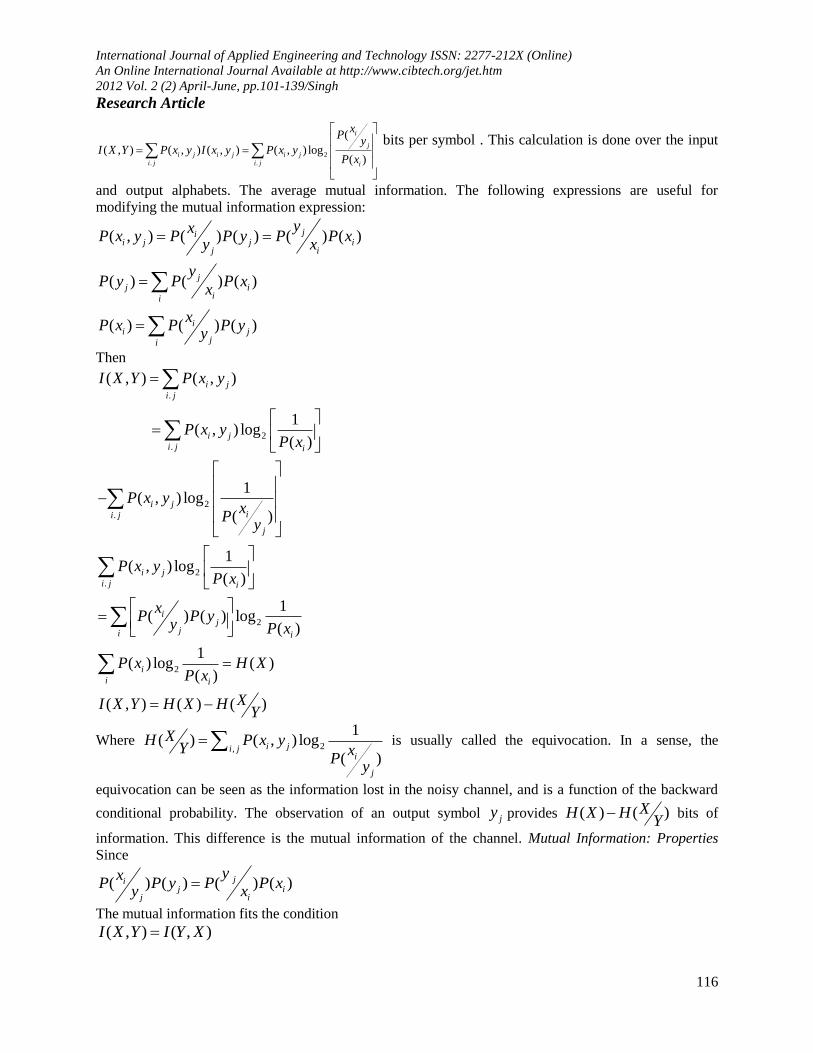
Mutual information measures the information transferred when ix is sent and iy is received, and is
defined as
2
( )
( , ) log (1)( )
i
ii i
i
xP
yI x y bits
P x
In a noise-free channel, each iy is uniquely connected to the corresponding ix , and so they constitute an
input –output pair ( , )i ix y for which
2
1( ) 1 ( , ) log
( )i
i jj
i
xP and I x y
y P x bits; that is, the transferred information is equal to the self-
information that corresponds to the input ix In a very noisy channel, the output iy and input ix would be
completely uncorrelated, and so ( ) ( )ii
j
xP P x
y and also ( , ) 0;i jI x y that is, there is no transference
of information. In general, a given channel will operate between these two extremes. The mutual
information is defined between the input and the output of a given channel. An average of the calculation
of the mutual information for all input-output pairs of a given channel is the average mutual information:
International Journal of Applied Engineering and Technology ISSN: 2277-212X (Online)
An Online International Journal Available at http://www.cibtech.org/jet.htm
2012 Vol. 2 (2) April-June, pp.101-139/Singh
Research Article
116
2
. .
(
( , ) ( , ) ( , ) ( , ) log( )
i
j
i j i j i j
i j i j i
xP
yI X Y P x y I x y P x y
P x
bits per symbol . This calculation is done over the input
and output alphabets. The average mutual information. The following expressions are useful for
modifying the mutual information expression:
( , ) ( ) ( ) ( ) ( )
( ) ( ) ( )
( ) ( ) ( )
jii j j i
j i
jj i
ii
ii j
ji
yxP x y P P y P P x
y x
yP y P P x
x
xP x P P y
y
Then
.
2
.
2
.
2
.
2
2
( , ) ( , )
1( , ) log
( )
1( , ) log
( )
1( , ) log
( )
1( ) ( ) log
( )
1( ) log ( )
( )
( , ) ( ) ( )
i j
i j
i j
i j i
i jii j
j
i j
i j i
ij
ji i
i
i i
I X Y P x y
P x yP x
P x yx
Py
P x yP x
xP P y
y P x
P x H XP x
XI X Y H X HY
Where 2,
1( ) ( , ) log
( )i ji j
i
j
XH P x yY x
Py
is usually called the equivocation. In a sense, the
equivocation can be seen as the information lost in the noisy channel, and is a function of the backward
conditional probability. The observation of an output symbol jy provides ( ) ( )XH X HY
bits of
information. This difference is the mutual information of the channel. Mutual Information: Properties
Since
( ) ( ) ( ) ( )jij i
j i
yxP P y P P x
y x
The mutual information fits the condition
( , ) ( , )I X Y I Y X
International Journal of Applied Engineering and Technology ISSN: 2277-212X (Online)
An Online International Journal Available at http://www.cibtech.org/jet.htm
2012 Vol. 2 (2) April-June, pp.101-139/Singh
Research Article
117
And by interchanging input and output it is also true that
( , ) ( ) ( )YI X Y H Y HX
Where
2
1( ) ( ) log
( )j
j j
H Y P yP y
This last entropy is usually called the noise entropy. Thus, the information transferred through the channel
is the difference between the output entropy and the noise entropy. Alternatively, it can be said that the
channel mutual information is the difference between the number of bits needed for determining a given
input symbol before knowing the corresponding output symbol, and the number of bits needed for
determining a given input symbol after knowing the corresponding output symbol
( , ) ( ) ( )XI X Y H X HY
As the channel mutual information expression is a difference between two quantities, it seems that this
parameter can adopt negative values. However, and is spite of the fact that for some , ( / )j jy H X y can
be larger than ( )H X , this is not possible for the average value calculated over all the outputs:
2 2
, ,
( )( , )
( , ) log ( , ) log( ) ( ) ( )
i
j i j
i j i j
i j i ji i j
xP
y P x yP x y P x y
P x P x P y
Then
,
( ) ( )( , ) ( , ) 0
( , )
i j
i j
i j i j
P x P yI X Y P x y
P x y
Because this expression is of the form
2
1
log ( ) 0M
ii
i i
QP
P
The above expression can be applied due to the factor ( ) ( ),i jP x P y which is the product of two
probabilities, so that it behaves as the quantity iQ , which in this expression is a dummy variable that fits
the condition 1iiQ . It can be concluded that the average mutual information is a non-negative
number. It can also be equal to zero, when the input and the output are independent of each other. A
related entropy called the joint entropy is defined as
2
,
2
,
2
,
1( , ) ( , ) log
( , )
( ) ( )( , ) log
( , )
1( , ) log
( ) ( )
i j
i j i j
i j
i j
i j i j
i j
i j i j
H X Y P x yP x y
P x P yP x y
P x y
P x yP x P y
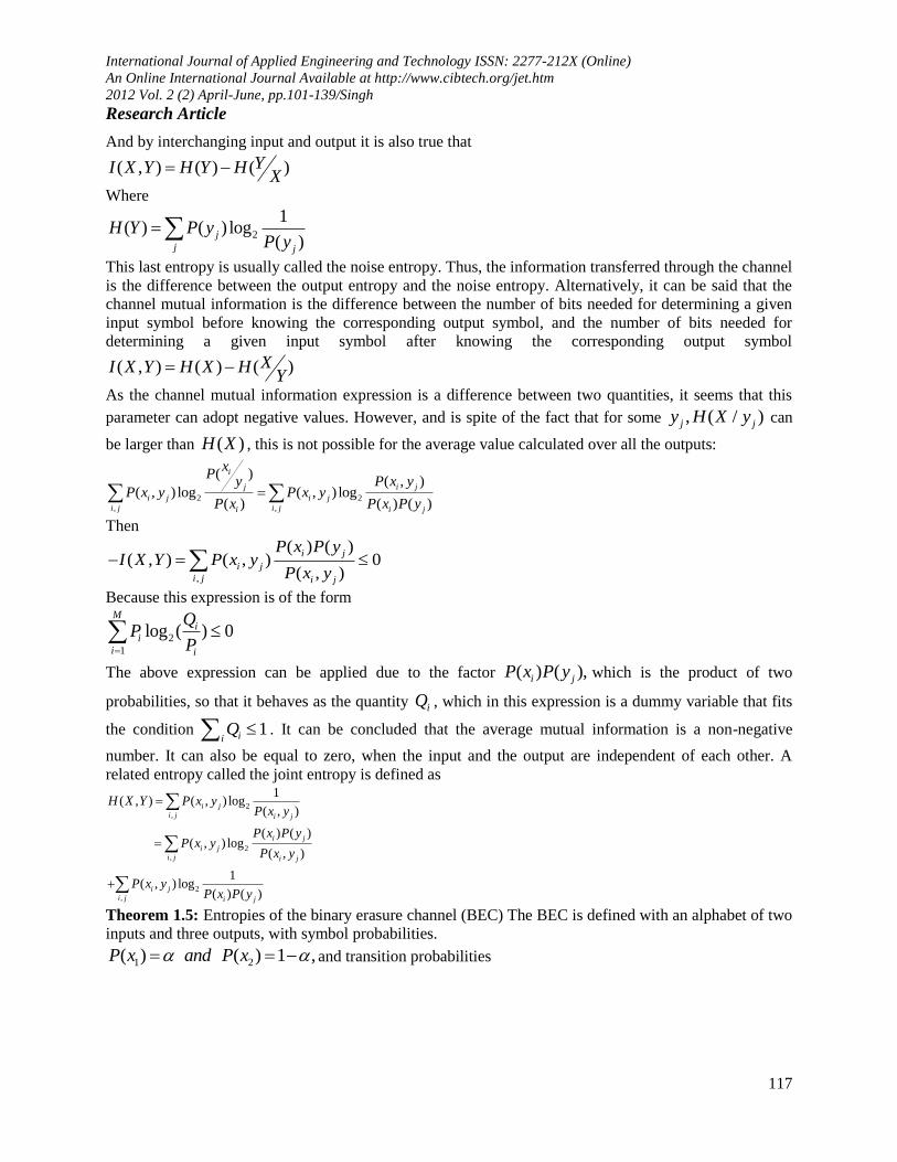
Theorem 1.5: Entropies of the binary erasure channel (BEC) The BEC is defined with an alphabet of two
inputs and three outputs, with symbol probabilities.
1 2( ) ( ) 1 ,P x and P x and transition probabilities
International Journal of Applied Engineering and Technology ISSN: 2277-212X (Online)
An Online International Journal Available at http://www.cibtech.org/jet.htm
2012 Vol. 2 (2) April-June, pp.101-139/Singh
Research Article
118
3 2
2 1
3
1
1
2
3
2
( ) 1 ( ) 0,
( ) 0
( )
( ) 1
y yP p and P
x x
yand P
x
yand P p
x
yand P p
x
Lemma 1.7. Given an arbitrary restricted time-discrete, amplitude-continuous channel whose restrictions
are determined by sets nF and whose density functions exhibit no dependence on the state s , let n be a
fixed positive integer, and ( )p x an arbitrary probability density function on Euclidean n-space. ( | )p y x
for the density 1 1( ,..., | ,... )n n np y y x x and nF for F. For any real number a, let
( | )( , ) : log (1)
( )
p y xA x y a
p y
Then for each positive integer u , there is a code ( , , )u n such that
( , ) (2)aue P X Y A P X F
Where
( , ) ... ( , ) , ( , ) ( ) ( | )
... ( )
A
F
P X Y A p x y dxdy p x y p x p y x
and
P X F p x dx
Proof: A sequence (1)x F such that
1
(1)| 1
: ( , ) ;
x
x
P Y A X x
where A y x y A
Choose the decoding set 1B to be (1)xA . Having chosen
(1) ( 1),........, kx x and 1 1,..., kB B , select
kx F
such that
( )
1( )
1
| 1 ;k
kk
ixi
P Y A B X x
Set ( )
1
1k
k
k ix iB A B
, If the process does not terminate in a finite number of steps, then the sequences
( )ix and decoding sets , 1,2,..., ,iB i u form the desired code. Thus assume that the process terminates
after t steps. (Conceivably 0t ). We will show t u by showing that
( , )ate P X Y A P X F . We proceed as follows.
Let
1
( , )
. ( 0, ).
( , ) ( , )
( ) ( | )
( ) ( | ) ( )
x
x
t
jj
x y A
x y A
x y B A x
B B If t take B Then
P X Y A p x y dx dy
p x p y x dy dx
p x p y x dy dx p x
International Journal of Applied Engineering and Technology ISSN: 2277-212X (Online)
An Online International Journal Available at http://www.cibtech.org/jet.htm
2012 Vol. 2 (2) April-June, pp.101-139/Singh
Research Article
119
C. Algorithms
Ideals. Let A be a ring. Recall that an ideal a in A is a subset such that a is subgroup of A regarded as a
group under addition;
,a a r A ra A
The ideal generated by a subset S of A is the intersection of all ideals A containing a ----- it is easy to
verify that this is in fact an ideal, and that it consist of all finite sums of the form i i
r s with
,i ir A s S . When 1,....., mS s s , we shall write 1( ,....., )ms s for the ideal it generates.
Let a and b be ideals in A. The set | ,a b a a b b is an ideal, denoted by a b . The ideal
generated by | ,ab a a b b is denoted by ab . Note that ab a b . Clearly ab consists of all
finite sums i i
a b with ia a and ib b , and if 1( ,..., )ma a a and 1( ,..., )nb b b , then
1 1( ,..., ,..., )i j m nab a b a b a b .Let a be an ideal of A. The set of cosets of a in A forms a ring /A a , and
a a a is a homomorphism : /A A a . The map 1( )b b is a one to one correspondence
between the ideals of /A a and the ideals of A containing a An ideal p if prime if p A and
ab p a p or b p . Thus p is prime if and only if /A p is nonzero and has the property that
0, 0 0,ab b a i.e., /A p is an integral domain. An ideal m is maximal if |m A and
there does not exist an ideal n contained strictly between m and A . Thus m is maximal if and only if
/A m has no proper nonzero ideals, and so is a field. Note that m maximal m prime. The ideals of
A B are all of the form a b , with a and b ideals in A and B . To see this, note that if c is an ideal
in A B and ( , )a b c , then ( ,0) ( , )(1,0)a a b c and (0, ) ( , )(0,1)b a b c . This shows that
c a b with
| ( , )a a a b c some b b
and
| ( , )b b a b c some a a
Let A be a ring. An A -algebra is a ring B together with a homomorphism :Bi A B . A
homomorphism of A -algebra B C is a homomorphism of rings : B C such that
( ( )) ( )B Ci a i a for all . An A -algebra B is said to be finitely generated ( or of finite-type over
A) if there exist elements 1,..., nx x B such that every element of B can be expressed as a polynomial in
the ix with coefficients in ( )i A , i.e., such that the homomorphism 1,..., nA X X B sending iX to
ix is surjective. A ring homomorphism A B is finite, and B is finitely generated as an A-module. Let
k be a field, and let A be a k -algebra. If 1 0 in A , then the map k A is injective, we can identify
k with its image, i.e., we can regard k as a subring of A . If 1=0 in a ring R, the R is the zero ring, i.e.,
0R . Polynomial rings. Let k be a field. A monomial in 1,..., nX X is an expression of the form
1
1 ... ,naa
n jX X a N . The total degree of the monomial is ia . We sometimes abbreviate it by
1, ( ,..., ) n
nX a a .
The elements of the polynomial ring 1,..., nk X X are finite sums
1
1 1.... 1 ....... , ,n
n n
aa
a a n a a jc X X c k a
a A
International Journal of Applied Engineering and Technology ISSN: 2277-212X (Online)
An Online International Journal Available at http://www.cibtech.org/jet.htm
2012 Vol. 2 (2) April-June, pp.101-139/Singh
Research Article
120
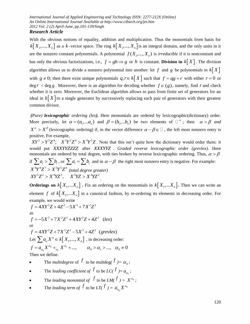
With the obvious notions of equality, addition and multiplication. Thus the monomials from basis for
1,..., nk X X as a k -vector space. The ring 1,..., nk X X is an integral domain, and the only units in it
are the nonzero constant polynomials. A polynomial 1( ,..., )nf X X is irreducible if it is nonconstant and
has only the obvious factorizations, i.e., f gh g or h is constant. Division in k X . The division
algorithm allows us to divide a nonzero polynomial into another: let f and g be polynomials in k X
with 0;g then there exist unique polynomials ,q r k X such that f qg r with either 0r or
deg r < deg g . Moreover, there is an algorithm for deciding whether ( )f g , namely, find r and check
whether it is zero. Moreover, the Euclidean algorithm allows to pass from finite set of generators for an
ideal in k X to a single generator by successively replacing each pair of generators with their greatest
common divisor.
(Pure) lexicographic ordering (lex). Here monomials are ordered by lexicographic(dictionary) order.
More precisely, let 1( ,... )na a and 1( ,... )nb b be two elements of n ; then and
X X (lexicographic ordering) if, in the vector difference , the left most nonzero entry is
positive. For example,
2 3 4 3 2 4 3 2;XY Y Z X Y Z X Y Z . Note that this isn’t quite how the dictionary would order them: it
would put XXXYYZZZZ after XXXYYZ . Graded reverse lexicographic order (grevlex). Here
monomials are ordered by total degree, with ties broken by reverse lexicographic ordering. Thus,
if i ia b , or i ia b and in the right most nonzero entry is negative. For example:
4 4 7 5 5 4X Y Z X Y Z (total degree greater) 5 2 4 3 5 4 2,XY Z X YZ X YZ X YZ .
Orderings on 1,... nk X X . Fix an ordering on the monomials in 1,... nk X X . Then we can write an
element f of 1,... nk X X in a canonical fashion, by re-ordering its elements in decreasing order. For
example, we would write 2 2 3 2 24 4 5 7f XY Z Z X X Z
as
3 2 2 2 25 7 4 4 ( )f X X Z XY Z Z lex or
2 2 2 3 24 7 5 4 ( )f XY Z X Z X Z grevlex
Let 1,..., na X k X X
, in decreasing order:
0 1
0 1 0 1 0..., ..., 0f a X X
Then we define.
The multidegree of f to be multdeg( f )= 0 ;
The leading coefficient of f to be LC( f )=0
a ;
The leading monomial of f to be LM( f ) = 0X
;
The leading term of f to be LT( f ) = 0
0a X
International Journal of Applied Engineering and Technology ISSN: 2277-212X (Online)
An Online International Journal Available at http://www.cibtech.org/jet.htm
2012 Vol. 2 (2) April-June, pp.101-139/Singh
Research Article
121
For the polynomial 24 ...,f XY Z the multidegree is (1,2,1), the leading coefficient is 4, the leading
monomial is 2XY Z , and the leading term is
24XY Z . The division algorithm in 1,... nk X X . Fix a
monomial ordering in 2 . Suppose given a polynomial f and an ordered set 1( ,... )sg g of polynomials;
the division algorithm then constructs polynomials 1,... sa a and r such that 1 1 ... s sf a g a g r
Where either 0r or no monomial in r is divisible by any of 1( ),..., ( )sLT g LT g Step 1: If
1( ) | ( )LT g LT f , divide 1g into f to get 1 1 1 1
1
( ), ,...,
( )n
LT ff a g h a k X X
LT g
If
1( ) | ( )LT g LT h , repeat the process until
1 1 1f a g f (different 1a ) with 1( )LT f not divisible by
1( )LT g . Now divide 2g into 1f , and so on,
until 1 1 1... s sf a g a g r With 1( )LT r not divisible by any 1( ),... ( )sLT g LT g Step 2: Rewrite
1 1 2( )r LT r r , and repeat Step 1 with 2r for f : 1 1 1 3... ( )s sf a g a g LT r r (different 'ia s )
Monomial ideals. In general, an ideal a will contain a polynomial without containing the individual
terms of the polynomial; for example, the ideal 2 3( )a Y X contains
2 3Y X but not 2Y or
3X .
DEFINITION 1.5. An ideal a is monomial if c X a X a
all with 0c .
PROPOSITION 1.3. Let a be a monomial ideal, and let |A X a . Then A satisfies the
condition , ( )nA And a is the k -subspace of 1,..., nk X X generated
by the ,X A . Conversely, of A is a subset of n satisfying , then the k-subspace a of
1,..., nk X X generated by |X A is a monomial ideal.
PROOF. It is clear from its definition that a monomial ideal a is the k -subspace of 1,..., nk X X
generated by the set of monomials it contains. If X a
and 1,..., nX k X X
.
If a permutation is chosen uniformly and at random from the !n possible permutations in ,nS then the
counts ( )n
jC of cycles of length j are dependent random variables. The joint distribution of
( ) ( ) ( )
1( ,..., )n n n
nC C C follows from Cauchy’s formula, and is given by
( )
1 1
1 1 1[ ] ( , ) 1 ( ) , (1.1)
! !
j
nncn
j
j j j
P C c N n c jc nn j c
for nc .
Lemma1.7 For nonnegative integers 1,...,
[ ]( )
11 1
,
1( ) 1 (1.4)
j
j
n
mn n n
mn
j j
jj j
m m
E C jm nj
International Journal of Applied Engineering and Technology ISSN: 2277-212X (Online)
An Online International Journal Available at http://www.cibtech.org/jet.htm
2012 Vol. 2 (2) April-June, pp.101-139/Singh
Research Article
122
Proof. This can be established directly by exploiting cancellation of the form [ ] !/ 1/ ( )!jm
j j j jc c c m
when ,j jc m which occurs between the ingredients in Cauchy’s formula and the falling factorials in the
moments. Write jm jm . Then, with the first sum indexed by 1( ,... ) n
nc c c and the last sum
indexed by 1( ,..., ) n
nd d d via the correspondence ,j j jd c m we have
[ ] [ ]( ) ( )
1 1
[ ]
: 1 1
11 1
( ) [ ] ( )
( )1
!
1 11
( )!
j j
j
j
j j
j j
n nm mn n
j j
cj j
mnn
j
j cc c m for all j j j j
n nn
jm dd jj j j
E C P C c c
cjc n
j c
jd n mj j d
This last sum simplifies to the indicator 1( ),m n corresponding to the fact that if 0,n m then
0jd for ,j n m and a random permutation in n mS must have some cycle structure 1( ,..., )n md d .
The moments of ( )n
jC follow immediately as
( ) [ ]( ) 1 (1.2)n r r
jE C j jr n
We note for future reference that (1.4) can also be written in the form
[ ] [ ]( )
11 1
( ) 1 , (1.3)j j
n n nm mn
j j j
jj j
E C E Z jm n
Where the jZ are independent Poisson-distribution random variables that satisfy ( ) 1/jE Z j
The marginal distribution of cycle counts provides a formula for the joint distribution of the cycle counts
,n
jC we find the distribution of n
jC using a combinatorial approach combined with the inclusion-
exclusion formula.
Lemma 1.8. For 1 ,j n
[ / ]
( )
0
[ ] ( 1) (1.1)! !
k ln j kn l
j
l
j jP C k
k l
Proof. Consider the set I of all possible cycles of length ,j formed with elements chosen from
1,2,... ,n so that [ ]/j jI n . For each ,I consider the “property” G of having ; that is, G is
the set of permutations nS such that is one of the cycles of . We then have ( )!,G n j
since the elements of 1,2,...,n not in must be permuted among themselves. To use the inclusion-
exclusion formula we need to calculate the term ,rS which is the sum of the probabilities of the r -fold
intersection of properties, summing over all sets of r distinct properties. There are two cases to consider.
If the r properties are indexed by r cycles having no elements in common, then the intersection specifies
how rj elements are moved by the permutation, and there are ( )!1( )n rj rj n permutations in the
intersection. There are [ ] / ( !)rj rn j r such intersections. For the other case, some two distinct properties
name some element in common, so no permutation can have both these properties, and the r -fold
intersection is empty. Thus
International Journal of Applied Engineering and Technology ISSN: 2277-212X (Online)
An Online International Journal Available at http://www.cibtech.org/jet.htm
2012 Vol. 2 (2) April-June, pp.101-139/Singh
Research Article
123
[ ]
( )!1( )
1 11( )
! ! !
r
rj
r r
S n rj rj n
nrj n
j r n j r
Finally, the inclusion-exclusion series for the number of permutations having exactly k properties is
,
0
( 1)l
k l
l
k lS
l
Which simplifies to (1.1) Returning to the original hat-check problem, we substitute j=1 in (1.1) to obtain
the distribution of the number of fixed points of a random permutation. For 0,1,..., ,k n
( )
1
0
1 1[ ] ( 1) , (1.2)
! !
n kn l
l
P C kk l
and the moments of ( )
1
nC follow from (1.2) with 1.j In particular, for 2,n the mean and variance
of ( )
1
nC are both equal to 1. The joint distribution of ( ) ( )
1( ,..., )n n
bC C for any 1 b n has an expression
similar to (1.7); this too can be derived by inclusion-exclusion. For any 1( ,..., ) b
bc c c with
,im ic
1
( ) ( )
1
...
01 1
[( ,..., ) ]
1 1 1 1( 1) (1.3)
! !
i i
b
i
n n
b
c lb bl l
l withi ii iil n m
P C C c
i c i l
The joint moments of the first b counts ( ) ( )
1 ,...,n n
bC C can be obtained directly from (1.2) and (1.3) by
setting 1 ... 0b nm m
The limit distribution of cycle counts
It follows immediately from Lemma 1.2 that for each fixed ,j as ,n
( ) 1/[ ] , 0,1,2,...,!
kn j
j
jP C k e k
k
So that ( )n
jC converges in distribution to a random variable jZ having a Poisson distribution with mean
1/ ;j we use the notation ( )n
j d jC Z where (1/ )j oZ P j to describe this. Infact, the limit random
variables are independent.
Theorem 1.6 The process of cycle counts converges in distribution to a Poisson process of with
intensity 1j . That is, as ,n
( ) ( )
1 2 1 2( , ,...) ( , ,...) (1.1)n n
dC C Z Z
Where the , 1,2,...,jZ j are independent Poisson-distributed random variables with 1
( )jE Zj
Proof. To establish the converges in distribution one shows that for each fixed 1,b as ,n
( ) ( )
1 1[( ,..., ) ] [( ,..., ) ]n n
b bP C C c P Z Z c
International Journal of Applied Engineering and Technology ISSN: 2277-212X (Online)
An Online International Journal Available at http://www.cibtech.org/jet.htm
2012 Vol. 2 (2) April-June, pp.101-139/Singh
Research Article
124
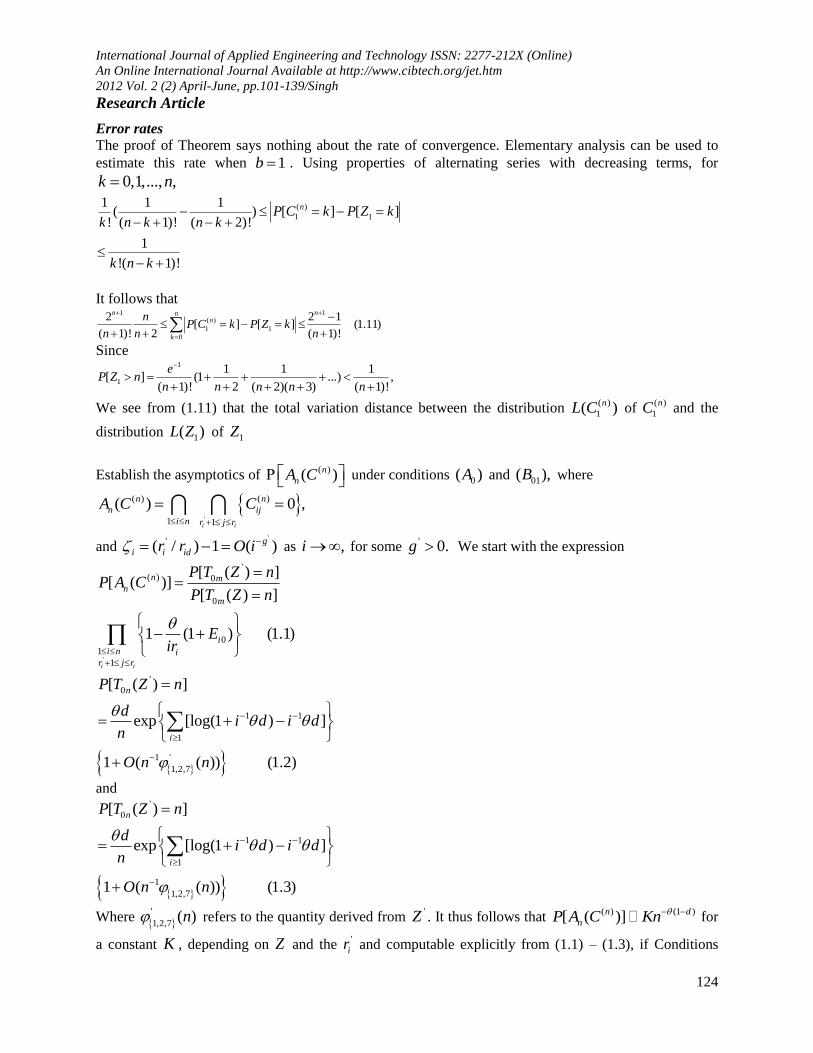
Error rates
The proof of Theorem says nothing about the rate of convergence. Elementary analysis can be used to
estimate this rate when 1b . Using properties of alternating series with decreasing terms, for
0,1,..., ,k n
( )
1 1
1 1 1( ) [ ] [ ]
! ( 1)! ( 2)!
1
!( 1)!
nP C k P Z kk n k n k
k n k
It follows that 1 1
( )
1 1
0
2 2 1[ ] [ ] (1.11)
( 1)! 2 ( 1)!
n nnn
k
nP C k P Z k
n n n
Since 1
1
1 1 1[ ] (1 ...) ,
( 1)! 2 ( 2)( 3) ( 1)!
eP Z n
n n n n n
We see from (1.11) that the total variation distance between the distribution ( )
1( )nL C of ( )
1
nC and the
distribution 1( )L Z of 1Z
Establish the asymptotics of ( )( )n
nA C under conditions 0( )A and 01( ),B where
'
( ) ( )
1 1
( ) 0 ,
i i
n n
n ij
i n r j r
A C C
and ''( / ) 1 ( )g
i i idr r O i as ,i for some ' 0.g We start with the expression
'
'( ) 0
0
0
1
1
[ ( ) ][ ( )]
[ ( ) ]
1 (1 ) (1.1)
i i
n mn
m
i
i n ir j r
P T Z nP A C
P T Z n
Eir
'
0
1 1
1
1 '
1,2,7
[ ( ) ]
exp [log(1 ) ]
1 ( ( )) (1.2)
n
i
P T Z n
di d i d
n
O n n
and
'
0
1 1
1
1
1,2,7
[ ( ) ]
exp [log(1 ) ]
1 ( ( )) (1.3)
n
i
P T Z n
di d i d
n
O n n
Where '
1,2,7( )n refers to the quantity derived from
'Z . It thus follows that ( ) (1 )[ ( )]n d
nP A C Kn for
a constant K , depending on Z and the '
ir and computable explicitly from (1.1) – (1.3), if Conditions
International Journal of Applied Engineering and Technology ISSN: 2277-212X (Online)
An Online International Journal Available at http://www.cibtech.org/jet.htm
2012 Vol. 2 (2) April-June, pp.101-139/Singh
Research Article
125
0( )A and 01( )B are satisfied and if '
( )g
i O i from some ' 0,g since, under these circumstances,
both
1 '
1,2,7( )n n and
1
1,2,7( )n n tend to zero as .n In particular, for polynomials and square
free polynomials, the relative error in this asymptotic approximation is of order 1n if
' 1.g
For 0 / 8b n and 0 ,n n with 0n
7,7
( ( [1, ]), ( [1, ]))
( ( [1, ]), ( [1, ]))
( , ),
TV
TV
d L C b L Z b
d L C b L Z b
n b
Where 7,7( , ) ( / )n b O b n under Conditions 0 1( ), ( )A D and 11( )B
Since, by the Conditioning
Relation, 0 0( [1, ] | ( ) ) ( [1, ] | ( ) ),b bL C b T C l L Z b T Z l
It follows by direct calculation that
0 0
0
0
( ( [1, ]), ( [1, ]))
( ( ( )), ( ( )))
max [ ( ) ]
[ ( ) ]1 (1.4)
[ ( ) ]
TV
TV b b
bA
r A
bn
n
d L C b L Z b
d L T C L T Z
P T Z r
P T Z n r
P T Z n
Suppressing the argument Z from now on, we thus obtain
( ( [1, ]), ( [1, ]))TVd L C b L Z b
0
0 0
[ ][ ] 1
[ ]
bnb
r n
P T n rP T r
P T n
[ /2]
00
/2 0 0
[ ][ ]
[ ]
n
bb
r n r b
P T rP T r
P T n
0
0
[ ]( [ ] [ ]n
b bn bn
s
P T s P T n s P T n r
[ /2]
0 0
/2 0
[ ] [ ]n
b b
r n r
P T r P T r
[ /2]
0
0 0
[ /2]
0 0
0 [ /2] 1
[ ] [ ][ ]
[ ]
[ ] [ ] [ ] / [ ]
nbn bn
b
s n
n n
b bn n
s s n
P T n s P T n rP T s
P T n
P T r P T s P T n s P T n
The first sum is at most 1
02 ;bn ETthe third is
bound by
International Journal of Applied Engineering and Technology ISSN: 2277-212X (Online)
An Online International Journal Available at http://www.cibtech.org/jet.htm
2012 Vol. 2 (2) April-June, pp.101-139/Singh
Research Article
126
0 0/2
10.5(1)
( max [ ]) / [ ]
2 ( / 2, ) 3,
[0,1]
b nn s n
P T s P T n
n b n
n P
[ /2] [ /2]2
0 010.80 0
10.8 0
3 14 ( ) [ ] [ ]
[0,1] 2
12 ( )
[0,1]
n n
b b
r s
b
nn n P T r P T s r s
P
n ET
P n
Hence we may take
10.81
07,7
10.5(1)
6 ( )( , ) 2 ( ) 1
[0,1]
6( / 2, ) (1.5)
[0,1]
b
nn b n ET Z P
P
n bP
Required order under Conditions 0 1( ), ( )A D and 11( ),B if ( ) .S If not, 10.8
n can be replaced
by 10.11
nin the above, which has the required order, without the restriction on the ir implied by
( )S . Examining the Conditions 0 1( ), ( )A D and 11( ),B it is perhaps surprising to find that 11( )B is
required instead of just 01( );B that is, that we should need 1
2( )a
illl O i
to hold for some 1 1a .
A first observation is that a similar problem arises with the rate of decay of 1i as well. For this reason,
1n is replaced by 1n
. This makes it possible to replace condition 1( )A by the weaker pair of conditions
0( )A and 1( )D in the eventual assumptions needed for 7,7
,n b to be of order ( / );O b n the decay
rate requirement of order 1i
is shifted from 1i itself to its first difference. This is needed to obtain the
right approximation error for the random mappings example. However, since all the classical applications
make far more stringent assumptions about the 1, 2,i l than are made in 11( )B . The critical point of the
proof is seen where the initial estimate of the difference( ) ( )[ ] [ 1]m m
bn bnP T s P T s . The factor
10.10( ),n which should be small, contains a far tail element from 1n
of the form 1 1( ) ( ),n u n which
is only small if 1 1,a being otherwise of order 11( )aO n for any 0, since 2 1a is in any case
assumed. For / 2,s n this gives rise to a contribution of order 11( )aO n in the estimate of the
difference [ ] [ 1],bn bnP T s P T s which, in the remainder of the proof, is translated into a
contribution of order 11( )aO tn for differences of the form [ ] [ 1],bn bnP T s P T s finally leading
to a contribution of order 1abn for any 0 in 7.7
( , ).n b Some improvement would seem to be
possible, defining the function g by ( ) 1 1 ,w s w s t
g w
differences that are of the form
[ ] [ ]bn bnP T s P T s t can be directly estimated, at a cost of only a single contribution of the form
International Journal of Applied Engineering and Technology ISSN: 2277-212X (Online)
An Online International Journal Available at http://www.cibtech.org/jet.htm
2012 Vol. 2 (2) April-June, pp.101-139/Singh
Research Article
127
1 1( ) ( ).n u n Then, iterating the cycle, in which one estimate of a difference in point probabilities is
improved to an estimate of smaller order, a bound of the form 112[ ] [ ] ( )a
bn bnP T s P T s t O n t n for any 0 could perhaps be attained, leading to a
final error estimate in order 11( )aO bn n for any 0 , to replace 7.7( , ).n b This would be of the
ideal order ( / )O b n for large enough ,b but would still be coarser for small .b
With b and n as in the previous section, we wish to show that
1
0 0
7,8
1( ( [1, ]), ( [1, ])) ( 1) 1
2
( , ),
TV b bd L C b L Z b n E T ET
n b
Where
121 1
7.8( , ) ( [ ])n b O n b n b n for any 0 under Conditions 0 1( ), ( )A D and 12( ),B with
12 . The proof uses sharper estimates. As before, we begin with the formula
0
0 0
( ( [1, ]), ( [1, ]))
[ ][ ] 1
[ ]
TV
bnb
r n
d L C b L Z b
P T n rP T r
P T n
Now we observe that
[ /2]
00
0 00 0
0
[ /2] 1
2 2
0 0 0/2
0
10.5(2)2 2
0
[ ] [ ][ ] 1
[ ] [ ]
[ ]( [ ] [ ])
4 ( max [ ]) / [ ]
[ / 2]
3 ( / 2, )8 , (1.1)
[0,1]
n
bn bb
r rn n
n
b bn bn
s n
b b nn s n
b
b
P T n r P T rP T r
P T n P T n
P T s P T n s P T n r
n ET P T s P T n
P T n
n bn ET
P
We have
0[ /2]
0
0
[ /2]
0
0
[ /2]
0 0
0
0 020 00
1
010.14 10.8
[ ]
[ ]
( [ ]( [ ] [ ]
( )(1 )[ ] [ ] )
1
1[ ] [ ]
[ ]
( , ) 2( ) 1 4 ( )
6
bn
n
r
n
b bn bn
s
n
b n
s
b b
r sn
P T r
P T n
P T s P T n s P T n r
s rP T s P T n
n
P T r P T s s rn P T n
n b r s n K n
0 10.14
2 2
0 0 10.8
( , )[0,1]
4 1 4 ( )
3( ) , (1.2)
[0,1]
b
b
ET n bnP
n ET K n
nP
International Journal of Applied Engineering and Technology ISSN: 2277-212X (Online)
An Online International Journal Available at http://www.cibtech.org/jet.htm
2012 Vol. 2 (2) April-June, pp.101-139/Singh
Research Article
128
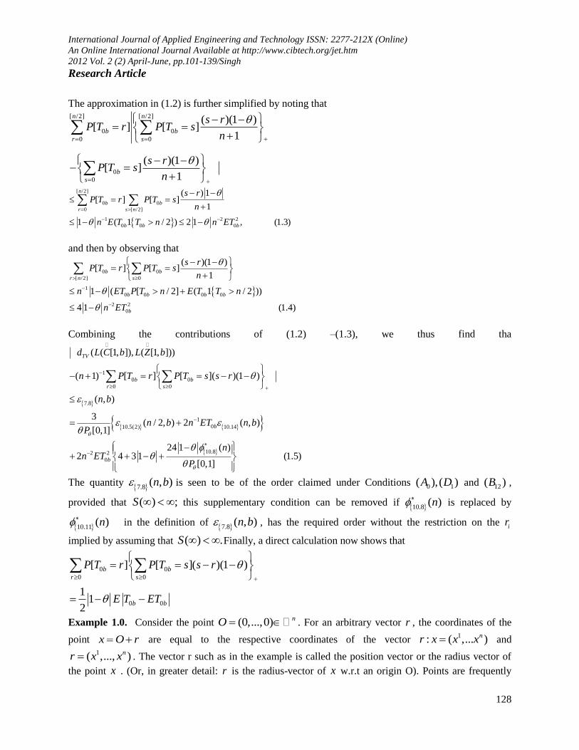
The approximation in (1.2) is further simplified by noting that [ /2] [ /2]
0 0
0 0
( )(1 )[ ] [ ]
1
n n
b b
r s
s rP T r P T s
n
0
0
( )(1 )[ ]
1b
s
s rP T s
n
[ /2]
0 0
0 [ /2]
1 2 2
0 0 0
( ) 1[ ] [ ]
1
1 ( 1 / 2 ) 2 1 , (1.3)
n
b b
r s n
b b b
s rP T r P T s
n
n E T T n n ET
and then by observing that
0 0
[ /2] 0
1
0 0 0 0
2 2
0
( )(1 )[ ] [ ]
1
1 ( [ / 2] ( 1 / 2 ))
4 1 (1.4)
b b
r n s
b b b b
b
s rP T r P T s
n
n ET P T n E T T n
n ET
Combining the contributions of (1.2) –(1.3), we thus find tha
1
0 0
0 0
7.8
1
010.5(2) 10.14
10.82 2
0
( ( [1, ]), ( [1, ]))
( 1) [ ] [ ]( )(1 )
( , )
3( / 2, ) 2 ( , )
[0,1]
24 1 ( )2 4 3 1 (1.5)
[0,1]
TV
b b
r s
b
b
d L C b L Z b
n P T r P T s s r
n b
n b n ET n bP
nn ET
P
The quantity 7.8( , )n b is seen to be of the order claimed under Conditions 0 1( ), ( )A D and 12( )B ,
provided that ( ) ;S this supplementary condition can be removed if 10.8
( )n is replaced by
10.11( )n
in the definition of 7.8( , )n b , has the required order without the restriction on the ir
implied by assuming that ( ) .S Finally, a direct calculation now shows that
0 0
0 0
0 0
[ ] [ ]( )(1 )
11
2
b b
r s
b b
P T r P T s s r
E T ET
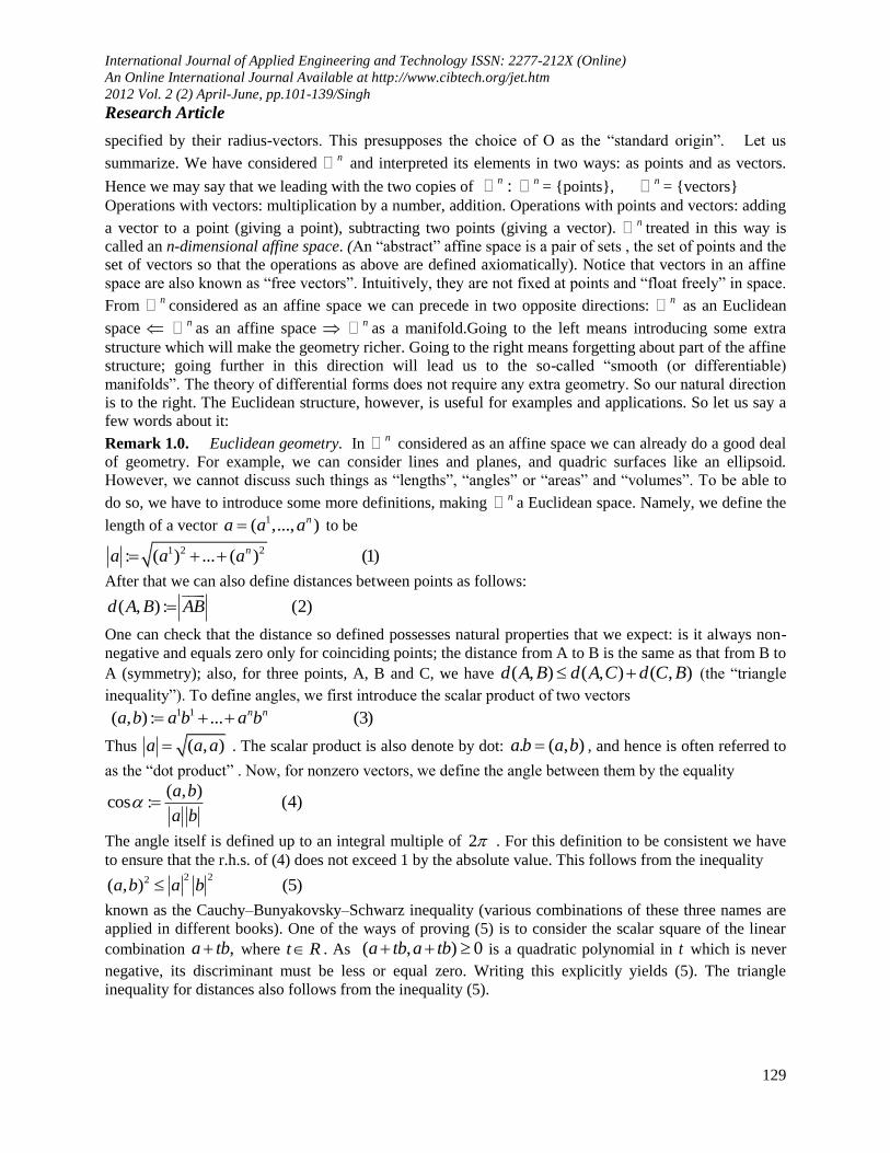
Example 1.0. Consider the point (0,...,0) nO . For an arbitrary vector r , the coordinates of the
point x O r are equal to the respective coordinates of the vector 1: ( ,... )nr x x x and
1( ,..., )nr x x . The vector r such as in the example is called the position vector or the radius vector of
the point x . (Or, in greater detail: r is the radius-vector of x w.r.t an origin O). Points are frequently
International Journal of Applied Engineering and Technology ISSN: 2277-212X (Online)
An Online International Journal Available at http://www.cibtech.org/jet.htm
2012 Vol. 2 (2) April-June, pp.101-139/Singh
Research Article
129
specified by their radius-vectors. This presupposes the choice of O as the “standard origin”. Let us
summarize. We have considered n and interpreted its elements in two ways: as points and as vectors.
Hence we may say that we leading with the two copies of :n n = {points},
n = {vectors}
Operations with vectors: multiplication by a number, addition. Operations with points and vectors: adding
a vector to a point (giving a point), subtracting two points (giving a vector). n treated in this way is
called an n-dimensional affine space. (An “abstract” affine space is a pair of sets , the set of points and the
set of vectors so that the operations as above are defined axiomatically). Notice that vectors in an affine
space are also known as “free vectors”. Intuitively, they are not fixed at points and “float freely” in space.
From n considered as an affine space we can precede in two opposite directions:
n as an Euclidean
space n as an affine space
n as a manifold.Going to the left means introducing some extra
structure which will make the geometry richer. Going to the right means forgetting about part of the affine
structure; going further in this direction will lead us to the so-called “smooth (or differentiable)
manifolds”. The theory of differential forms does not require any extra geometry. So our natural direction
is to the right. The Euclidean structure, however, is useful for examples and applications. So let us say a
few words about it:
Remark 1.0. Euclidean geometry. In n considered as an affine space we can already do a good deal
of geometry. For example, we can consider lines and planes, and quadric surfaces like an ellipsoid.
However, we cannot discuss such things as “lengths”, “angles” or “areas” and “volumes”. To be able to
do so, we have to introduce some more definitions, making n a Euclidean space. Namely, we define the
length of a vector 1( ,..., )na a a to be
1 2 2: ( ) ... ( ) (1)na a a
After that we can also define distances between points as follows:
( , ) : (2)d A B AB
One can check that the distance so defined possesses natural properties that we expect: is it always non-
negative and equals zero only for coinciding points; the distance from A to B is the same as that from B to
A (symmetry); also, for three points, A, B and C, we have ( , ) ( , ) ( , )d A B d A C d C B (the “triangle
inequality”). To define angles, we first introduce the scalar product of two vectors
1 1( , ) : ... (3)n na b a b a b
Thus ( , )a a a . The scalar product is also denote by dot: . ( , )a b a b , and hence is often referred to
as the “dot product” . Now, for nonzero vectors, we define the angle between them by the equality
( , )cos : (4)
a b
a b
The angle itself is defined up to an integral multiple of 2 . For this definition to be consistent we have
to ensure that the r.h.s. of (4) does not exceed 1 by the absolute value. This follows from the inequality 2 22( , ) (5)a b a b
known as the Cauchy–Bunyakovsky–Schwarz inequality (various combinations of these three names are
applied in different books). One of the ways of proving (5) is to consider the scalar square of the linear
combination ,a tb where t R . As ( , ) 0a tb a tb is a quadratic polynomial in t which is never
negative, its discriminant must be less or equal zero. Writing this explicitly yields (5). The triangle
inequality for distances also follows from the inequality (5).
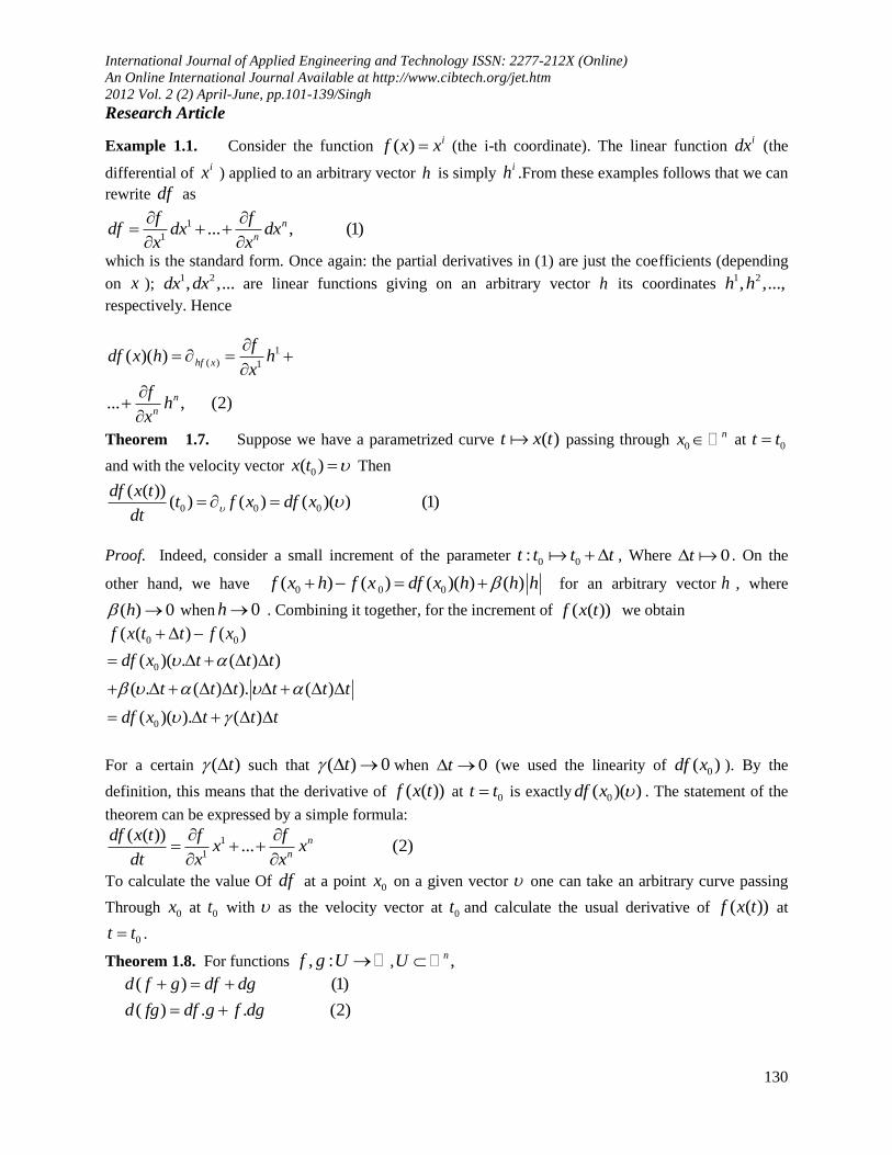
International Journal of Applied Engineering and Technology ISSN: 2277-212X (Online)
An Online International Journal Available at http://www.cibtech.org/jet.htm
2012 Vol. 2 (2) April-June, pp.101-139/Singh
Research Article
130
Example 1.1. Consider the function ( ) if x x (the i-th coordinate). The linear function idx (the
differential of ix ) applied to an arbitrary vector h is simply
ih .From these examples follows that we can
rewrite df as
1
1... , (1)n
n
f fdf dx dx
x x
which is the standard form. Once again: the partial derivatives in (1) are just the coefficients (depending
on x ); 1 2, ,...dx dx are linear functions giving on an arbitrary vector h its coordinates
1 2, ,...,h h
respectively. Hence
1
( ) 1( )( )
... , (2)
hf x
n
n
fdf x h h
x
fh
x
Theorem 1.7. Suppose we have a parametrized curve ( )t x t passing through 0
nx at 0t t
and with the velocity vector 0( )x t Then
0 0 0
( ( ))( ) ( ) ( )( ) (1)
df x tt f x df x
dt
Proof. Indeed, consider a small increment of the parameter 0 0:t t t t , Where 0t . On the
other hand, we have 0 0 0( ) ( ) ( )( ) ( )f x h f x df x h h h for an arbitrary vector h , where
( ) 0h when 0h . Combining it together, for the increment of ( ( ))f x t we obtain
0 0
0
0
( ( ) ( )
( )( . ( ) )
( . ( ) ). ( )
( )( ). ( )
f x t t f x
df x t t t
t t t t t t
df x t t t
For a certain ( )t such that ( ) 0t when 0t (we used the linearity of 0( )df x ). By the
definition, this means that the derivative of ( ( ))f x t at 0t t is exactly 0( )( )df x . The statement of the
theorem can be expressed by a simple formula:
1
1
( ( ))... (2)n
n
df x t f fx x
dt x x
To calculate the value Of df at a point 0x on a given vector one can take an arbitrary curve passing
Through 0x at 0t with as the velocity vector at 0t and calculate the usual derivative of ( ( ))f x t at
0t t .
Theorem 1.8. For functions , :f g U , ,nU
( ) (1)
( ) . . (2)
d f g df dg
d fg df g f dg
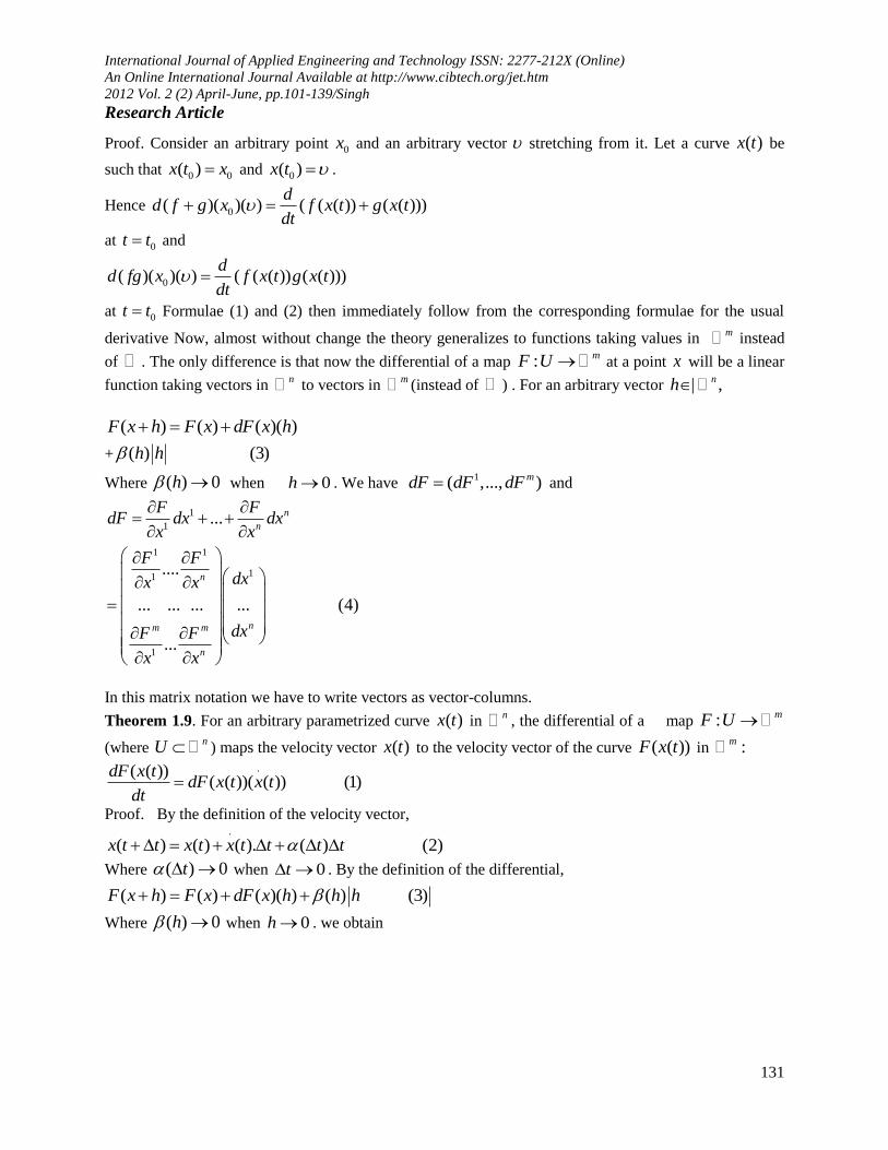
International Journal of Applied Engineering and Technology ISSN: 2277-212X (Online)
An Online International Journal Available at http://www.cibtech.org/jet.htm
2012 Vol. 2 (2) April-June, pp.101-139/Singh
Research Article
131
Proof. Consider an arbitrary point 0x and an arbitrary vector stretching from it. Let a curve ( )x t be
such that 0 0( )x t x and 0( )x t .
Hence 0( )( )( ) ( ( ( )) ( ( )))
dd f g x f x t g x t
dt
at 0t t and
0( )( )( ) ( ( ( )) ( ( )))d
d fg x f x t g x tdt
at 0t t Formulae (1) and (2) then immediately follow from the corresponding formulae for the usual
derivative Now, almost without change the theory generalizes to functions taking values in m instead
of . The only difference is that now the differential of a map : mF U at a point x will be a linear
function taking vectors in n to vectors in
m (instead of ) . For an arbitrary vector | ,nh
( ) ( ) ( )( )F x h F x dF x h
+ ( ) (3)h h
Where ( ) 0h when 0h . We have 1( ,..., )mdF dF dF and
1
1
1 1
11
1
...
....
... ... ... ... (4)
...
n
n
n
nm m
n
F FdF dx dx
x x
F F
dxx x
dxF F
x x
In this matrix notation we have to write vectors as vector-columns.
Theorem 1.9. For an arbitrary parametrized curve ( )x t in n , the differential of a map : mF U
(where nU ) maps the velocity vector ( )x t to the velocity vector of the curve ( ( ))F x t in :m
.( ( ))( ( ))( ( )) (1)
dF x tdF x t x t
dt
Proof. By the definition of the velocity vector, .
( ) ( ) ( ). ( ) (2)x t t x t x t t t t
Where ( ) 0t when 0t . By the definition of the differential,
( ) ( ) ( )( ) ( ) (3)F x h F x dF x h h h
Where ( ) 0h when 0h . we obtain
International Journal of Applied Engineering and Technology ISSN: 2277-212X (Online)
An Online International Journal Available at http://www.cibtech.org/jet.htm
2012 Vol. 2 (2) April-June, pp.101-139/Singh
Research Article
132
.
.
. .
.
( ( )) ( ( ). ( ) )
( ) ( )( ( ) ( ) )
( ( ) ( ) ). ( ) ( )
( ) ( )( ( ) ( )
h
F x t t F x x t t t t
F x dF x x t t t t
x t t t t x t t t t
F x dF x x t t t t
For some ( ) 0t when 0t . This precisely means that .
( ) ( )dF x x t is the velocity vector of
( )F x . As every vector attached to a point can be viewed as the velocity vector of some curve passing
through this point, this theorem gives a clear geometric picture of dF as a linear map on vectors.
Theorem 1.10 Suppose we have two maps :F U V and : ,G V W where
, ,n m pU V W (open domains). Let : ( )F x y F x . Then the differential of the
composite map :GoF U W is the composition of the differentials of F and :G
( )( ) ( ) ( ) (4)d GoF x dG y odF x
Proof. We can use the description of the differential .Consider a curve ( )x t in n with the velocity
vector .
x . Basically, we need to know to which vector in p it is taken by ( )d GoF . the curve
( )( ( ) ( ( ( ))GoF x t G F x t . By the same theorem, it equals the image under dG of the Anycast Flow
vector to the curve ( ( ))F x t in m . Applying the theorem once again, we see that the velocity vector to
the curve ( ( ))F x t is the image under dF of the vector .
( )x t . Hence . .
( )( ) ( ( ))d GoF x dG dF x for an
arbitrary vector .
x .
Corollary 1.0. If we denote coordinates in n by
1( ,..., )nx x and in m by
1( ,..., )my y , and write
1
1
1
1
... (1)
... , (2)
n
n
n
n
F FdF dx dx
x x
G GdG dy dy
y y
Then the chain rule can be expressed as follows:
1
1( ) ... , (3)m
m
G Gd GoF dF dF
y y
Where idF are taken from (1). In other words, to get ( )d GoF we have to substitute into (2) the
expression for i idy dF from (3). This can also be expressed by the following matrix formula:
1 1 1 1
11 1
1 1
.... ....
( ) ... ... ... ... ... ... ... (4)
... ...
m n
np p m m
m n
G G F F
dxy y x x
d GoF
dxG G F F
y y x x
International Journal of Applied Engineering and Technology ISSN: 2277-212X (Online)
An Online International Journal Available at http://www.cibtech.org/jet.htm
2012 Vol. 2 (2) April-June, pp.101-139/Singh
Research Article
133
i.e., if dG and dF are expressed by matrices of partial derivatives, then ( )d GoF is expressed by the
product of these matrices. This is often written as 1 11 1
11
1 1
1 1
1
1
........
... ... ... ... ... ...
... ...
....
... ... ... , (5)
...
mn
p p p p
n m
n
m m
n
z zz z
y yx x
z z z z
x x y y
y y
x x
y y
x x
Or
1
, (6)im
a i ai
z z y
x y x
Where it is assumed that the dependence of my on
nx is given by the map F , the dependence
of pz on
my is given by the map ,G and the dependence of pz on
nx is given by the
composition GoF .
Definition 1.6. Consider an open domain nU . Consider also another copy of
n , denoted for
distinction n
y , with the standard coordinates 1( ... )ny y . A system of coordinates in the open domain U
is given by a map : ,F V U where n
yV is an open domain of n
y , such that the following three
conditions are satisfied :
(1) F is smooth;
(2) F is invertible;
(3) 1 :F U V is also smooth
The coordinates of a point x U in this system are the standard coordinates of 1( ) n
yF x
In other words, 1 1: ( ..., ) ( ..., ) (1)n nF y y x x y y
Here the variables 1( ..., )ny y are the “new” coordinates of the point x
Example 1.2. Consider a curve in 2 specified in polar coordinates as
( ) : ( ), ( ) (1)x t r r t t
We can simply use the chain rule. The map ( )t x t can be considered as the composition of the maps
( ( ), ( )),( , ) ( , )t r t t r x r . Then, by the chain rule, we have
. . .
(2)dx x dr x d x x
x rdt r dt dt r
International Journal of Applied Engineering and Technology ISSN: 2277-212X (Online)
An Online International Journal Available at http://www.cibtech.org/jet.htm
2012 Vol. 2 (2) April-June, pp.101-139/Singh
Research Article
134
Here .
r and .
are scalar coefficients depending on t , whence the partial derivatives ,x xr
are
vectors depending on point in 2 . We can compare this with the formula in the “standard” coordinates:
. . .
1 2x e x e y . Consider the vectors ,x xr
. Explicitly we have
(cos ,sin ) (3)
( sin , cos ) (4)
x
r
xr r
From where it follows that these vectors make a basis at all points except for the origin (where 0r ). It
is instructive to sketch a picture, drawing vectors corresponding to a point as starting from that point.
Notice that ,x xr
are, respectively, the velocity vectors for the curves ( , )r x r
0( )fixed and 0( , ) ( )x r r r fixed . We can conclude that for an arbitrary curve given in
polar coordinates the velocity vector will have components . .
( , )r if as a basis we take
: , : :rx xe e
r
. . .
(5)rx e r e
A characteristic feature of the basis ,re e is that it is not “constant” but depends on point. Vectors “stuck
to points” when we consider curvilinear coordinates.
Proposition 1.3. The velocity vector has the same appearance in all coordinate systems.
Proof. Follows directly from the chain rule and the transformation law for the basis ie .In particular,
the elements of the basis iixe
x
(originally, a formal notation) can be understood directly as the
velocity vectors of the coordinate lines 1( ,..., )i nx x x x (all coordinates but
ix are fixed). Since we
now know how to handle velocities in arbitrary coordinates, the best way to treat the differential of a map
: n mF is by its action on the velocity vectors. By definition, we set
0 0 0
( ) ( ( ))( ) : ( ) ( ) (1)
dx t dF x tdF x t t
dt dt
Now 0( )dF x is a linear map that takes vectors attached to a point 0
nx to vectors attached to the
point ( ) mF x
1
1
1 1
11
1
1
...
...
( ,..., ) ... ... ... ... , (2)
...
n
n
n
m
nm m
n
F FdF dx dx
x x
F F
dxx x
e e
dxF F
x x
International Journal of Applied Engineering and Technology ISSN: 2277-212X (Online)
An Online International Journal Available at http://www.cibtech.org/jet.htm
2012 Vol. 2 (2) April-June, pp.101-139/Singh
Research Article
135
In particular, for the differential of a function we always have
1
1... , (3)n
n
f fdf dx dx
x x
Where ix are arbitrary coordinates. The form of the differential does not change when we perform a
change of coordinates.
Example 1.3 Consider a 1-form in 2 given in the standard coordinates:
A ydx xdy In the polar coordinates we will have cos , sinx r y r , hence
cos sin
sin cos
dx dr r d
dy dr r d
Substituting into A , we get
2 2 2 2
sin (cos sin )
cos (sin cos )
(sin cos )
A r dr r d
r dr r d
r d r d
Hence 2A r d is the formula for A in the polar coordinates. In particular, we see that this is again a
1-form, a linear combination of the differentials of coordinates with functions as coefficients. Secondly,
in a more conceptual way, we can define a 1-form in a domain U as a linear function on vectors at every
point of U : 1
1( ) ... , (1)n
n
If i
ie , where iixe
x
. Recall that the differentials of functions were defined as linear
functions on vectors (at every point), and ( ) (2)i i i
j jj
xdx e dx
x
at every point x .
Theorem 1.9. For arbitrary 1-form and path , the integral
does not change if we change
parametrization of provide the orientation remains the same.
Proof: Consider '
( ( )),dx
x tdt
and '
'( ( ( ))),
dxx t t
dt As
'
'( ( ( ))),
dxx t t
dt =
'
' '( ( ( ))), . ,
dx dtx t t
dt dt
Let p be a rational prime and let ( ).pK We write for p or this section. Recall that K has
degree ( ) 1p p over . We wish to show that .KO Note that is a root of 1,px and
thus is an algebraic integer; since K is a ring we have that .KO We give a proof without
assuming unique factorization of ideals. We begin with some norm and trace computations. Let j be an
integer. If j is not divisible by ,p then j is a primitive
thp root of unity, and thus its conjugates are
2 1, ,..., .p Therefore
2 1
/ ( ) ... ( ) 1 1j p
K pTr
If p does divide ,j then 1,j so it has only the one conjugate 1, and / ( ) 1j
KTr p By linearity
of the trace, we find that
International Journal of Applied Engineering and Technology ISSN: 2277-212X (Online)
An Online International Journal Available at http://www.cibtech.org/jet.htm
2012 Vol. 2 (2) April-June, pp.101-139/Singh
Research Article
136
2
/ /
1
/
(1 ) (1 ) ...
(1 )
K K
p
K
Tr Tr
Tr p
We also need to compute the norm of 1 . For this, we use the factorization
1 2
2 1
... 1 ( )
( )( )...( );
p p
p
p
x x x
x x x
Plugging in 1x shows that
2 1(1 )(1 )...(1 )pp
Since the (1 )j are the conjugates of (1 ), this shows that / (1 )KN p The key result for
determining the ring of integers KO is the following.
LEMMA 1.9
(1 ) KO p
Proof. We saw above that p is a multiple of (1 ) in ,KO so the inclusion (1 ) KO p is
immediate. Suppose now that the inclusion is strict. Since (1 ) KO is an ideal of containing
p and p is a maximal ideal of , we must have (1 ) KO Thus we can write
1 (1 )
For some .KO That is, 1 is a unit in .KO
COROLLARY 1.1 For any ,KO / ((1 ) ) .KTr p
PROOF. We have
/ 1 1
1 1 1 1
1
1 1
((1 ) ) ((1 ) ) ... ((1 ) )
(1 ) ( ) ... (1 ) ( )
(1 ) ( ) ... (1 ) ( )
K p
p p
p
p
Tr
Where the i are the complex embeddings of K (which we are really viewing as automorphisms of K )
with the usual ordering. Furthermore, 1 j is a multiple of 1 in KO for every 0.j Thus
/ ( (1 )) (1 )K KTr O Since the trace is also a rational integer.
PROPOSITION 1.4 Let p be a prime number and let | ( )pK be the thp cyclotomic field. Then
[ ] [ ] / ( ( ));K p pO x x Thus 21, ,..., p
p p is an integral basis for KO .
PROOF. Let KO and write
2
0 1 2... p
pa a a
With .ia Then
2
0 1
2 1
2
(1 ) (1 ) ( ) ...
( )p p
p
a a
a
By the linearity of the trace and our above calculations we find that / 0( (1 ))KTr pa We also
have
/ ( (1 )) ,KTr p so 0a Next consider the algebraic integer
International Journal of Applied Engineering and Technology ISSN: 2277-212X (Online)
An Online International Journal Available at http://www.cibtech.org/jet.htm
2012 Vol. 2 (2) April-June, pp.101-139/Singh
Research Article
137
1 3
0 1 2 2( ) ... ;p
pa a a a
This is an algebraic integer since 1 1p is. The same
argument as above shows that 1 ,a and continuing in this way we find that all of the ia are in .
This completes the proof.
Example 1.4 Let K , then the local ring ( )p is simply the subring of of rational numbers with
denominator relatively prime to p . Note that this ring ( )p is not the ring
p of p -adic integers; to get
p one must complete ( )p . The usefulness of
,K pO comes from the fact that it has a particularly simple
ideal structure. Let a be any proper ideal of ,K pO and consider the ideal Ka O of .KO We claim that
,( ) ;K K pa a O O That is, that a is generated by the elements of a in .Ka O It is clear from the
definition of an ideal that ,( ) .K K pa a O O To prove the other inclusion, let be any element of a .
Then we can write / where KO and .p In particular, a (since / a and a is
an ideal), so KO and .p so .Ka O Since ,1/ ,K pO this implies that
,/ ( ) ,K K pa O O as claimed.We can use this fact to determine all of the ideals of , .K pO Let a
be any ideal of ,K pO and consider the ideal factorization of Ka O in .KO write it as
n
Ka O p b For
some n and some ideal ,b relatively prime to .p we claim first that , , .K p K pbO O We now find that
, , ,( ) n n
K K p K p K pa a O O p bO p O Since , .K pbO Thus every ideal of
,K pO has the form ,
n
K pp O
for some ;n it follows immediately that ,K pO is noetherian. It is also now clear that ,
n
K pp O is the unique
non-zero prime ideal in ,K pO . Furthermore, the inclusion
, ,/K K p K pO O pO Since , ,K p KpO O p
this map is also surjection, since the residue class of ,/ K pO (with KO and p ) is the
image of 1
in / ,K pO which makes sense since is invertible in / .K pO Thus the map is an
isomorphism. In particular, it is now abundantly clear that every non-zero prime ideal of ,K pO is maximal.
To show that ,K pO is a Dedekind domain, it remains to show that it is integrally closed in K . So
let K be a root of a polynomial with coefficients in , ;K pO write this polynomial as
11 0
1 0
...m mm
m
x x
With i KO and .i K pO Set 0 1 1... .m Multiplying by m we
find that is the root of a monic polynomial with coefficients in .KO Thus ;KO since ,p
we have ,/ K pO . Thus
,K pO is integrally close in .K
COROLLARY 1.2. Let K be a number field of degree n and let be in KO then
'
/ /( ) ( )K K KN O N
PROOF. We assume a bit more Galois theory than usual for this proof. Assume first that /K is
Galois. Let be an element of ( / ).Gal K It is clear that /( ) / ( ) ;K KO O since ( ) ,K KO O
this shows that ' '
/ /( ( ) ) ( )K K K KN O N O . Taking the product over all ( / ),Gal K we have

International Journal of Applied Engineering and Technology ISSN: 2277-212X (Online)
An Online International Journal Available at http://www.cibtech.org/jet.htm
2012 Vol. 2 (2) April-June, pp.101-139/Singh
Research Article
138
' '
/ / /( ( ) ) ( )n
K K K K KN N O N O Since / ( )KN is a rational integer and KO is a free -module of
rank ,n
// ( )K K KO N O Will have order / ( ) ;n
KN therefore '
/ / /( ( ) ) ( )n
K K K K KN N O N O
This completes the proof. In the general case, let L be the Galois closure of K and set [ : ] .L K m
RESULTS
Two-dimensional cross-sectional images of in-vivo human skin tissues were successfully obtained by
employing lens scanning based MEMS endoscopic probe with SD-OCT system. An objective lens with
15 mm in working distance and 20 μm in lateral resolution is utilized for the deeper penetration depth.
The lateral scanning lens is actuated at the resonance frequency for two-dimensional imaging. Experiment
shows the axial resolution of the endoscopic SD-OCT system and the frequency response of the lens
scanner. The axial resolution of the system is measured to 7.7 μm in air, and the scanning area of 2.1 mm
is achieved at the resonant excitation at 122 Hz. Note that the heavy mass of the scanning lens
significantly increases the mechanical Q-factor, so it allows the low voltage operation at DC 3 V and AC
6 Vpp. As the beam moved along the scanning line, the generated interference spectra are spontaneously
obtained by a CMOS line scan camera. The camera acquisition rate is synchronized with the scanning
speed of the lens scanner, which corresponds to 62.5k A-lines/sec. The imaging speed of the system,
consequently, is 122frame/sec with pixel resolution of 256 x 1024 pixels (L x D). Experiment shows in-
vivo two-dimensional cross-sectional images of a human finger print and nail fold. Experiment shows the
detailed structures of the epidermis, the dermis, and the sweat gland of human palm. The four thin
laminated layers of the nail plate are shown in Experiment. The brightness and contrast in all images are
adjusted to show clear pictures.
CONCLUSIONS
In summary, the lens scanning based MEMS endoscopic catheter for forward imaging was designed,
assembled and integrated with high-speed SD-OCT system. Two different human tissue images were
successfully acquired by the endoscopic catheter. The current catheter has an outer dimension of 7 mm x
7 mm due to an objective lens diameter of 5 mm, while the MEM scanner with a scanning lens of 1mm in
diameter has 2.7 mm in width. Further reduction of the catheter size down to 5 mm work can be realized
by employing a miniaturized objective lens. This method provides small endoscopic packaging with large
aperture, body-safe low voltage operation, long working distances, and high-speed forward imaging
capability, therefore, it may provide new direction for examination for gastroscopic examination or 3D
forward imaging guided laparoscopic surgery. Authors and Affiliations
Dr Akash Singh is working with IBM Corporation as an IT Architect and has been designing Mission
Critical System and Service Solutions; He has published papers in IEEE and other International
Conferences and Journals.
He joined IBM in Jul 2003 as an IT Architect which conducts research and design of High Performance
Smart Grid Services and Systems and design mission critical architecture for High Performance
Computing Platform and Computational Intelligence and High Speed Communication systems. He is a
member of IEEE (Institute for Electrical and Electronics Engineers), the AAAI (Association for the
Advancement of Artificial Intelligence) and the AACR (American Association for Cancer Research). He is
the recipient of numerous awards from World Congress in Computer Science, Computer Engineering and
Applied Computing 2010, 2011, and IP Multimedia System 2008 and Billing and Roaming 2008. He is
active research in the field of Artificial Intelligence and advancement in Medical Systems. He is in
Industry for 18 Years where he performed various role to provide the Leadership in Information
Technology and Cutting edge Technology.

International Journal of Applied Engineering and Technology ISSN: 2277-212X (Online)
An Online International Journal Available at http://www.cibtech.org/jet.htm
2012 Vol. 2 (2) April-June, pp.101-139/Singh
Research Article
139
REFERENCES
Huang D, Swanson EA, Lin CP, Schuman JS, Stinson WG, Chang W, Hee M, Flotte T, Gregory K,
Puliafito C and Fujimoto J (1991). Optical coherence tomography. Science 254 1178-1181.
Tearney GJ, Brezinski ME, Bouma BE, Boppart BE, Pitris C, Southern JF and JG Fujimoto
(1997). In vivo endoscopic optical biopsy with optical coherence tomography. Science 276(5321) 2037–
2039.
Jung W, McCormick DT, Zhang J, Wang L, Tien NC, and Chen Z (2006). Three-dimensional
endoscopic optical coherence tomography by use of a two-axis microelectromechanical scanning mirror.
Applied Physics Letter 88(16) 163901.
Pan Y, Xie H, and Fedder GK (2001). Endoscopic optical coherence tomography based on a
microelectromechanical mirror. Optics Letter 26(24) 1996 -1998.
Sun J, Guo S, Wu L, Choe SW, Sorg BS and Xie H (2010). 3D In Vivo optical coherence tomography
based on a low-voltage large-scan-range 2D MEMS mirror. Optics Express 18(12) 12065-12075.
Kim KH, Park BH, Maguluri GN, Lee TW, Rogomentich FJ, Bancu MG, Bouma BE, de Boer JF
and Bernstein JJ (2007). Two-axis magnetically driven MEMS scanning catheter for endoscopic high-
speed optical coherence tomography. Optics Express 15(26) 18130-18140.
Liu X, Cobb MJ, Chen Y, Kimmey MB and Li X (2004). Rapid-scanning forward-imaging miniature
endoscope for real-time optical coherence tomography. Optics Letter 29(15) 1763-1765.
Huo L, Xi J, Wu Y and Li X (2010). Forward-viewing resonant fiber-optic scanning endoscope of
appropriate scanning speed for 3D OCT imaging. Optics Express 18(14) 14375-14384.
Wu T, Ding Z, Wang K, Chen M and Wang C (2009). Two-dimensional scanning realized by an
asymmetry fiber cantilever driven by single piezo bender actuator for optical coherence tomography.
Optics Express 17(16) 13819-13829.
Park HC, Song C and Jeong KH (2010). Micromachined lens microstages for two-dimensional forward
optical scanning. Optics Express 18(15) 16133-16138.
Wang RK and Ma Z (2006). A practical approach to eliminate autocorrelation artifacts for volume-rate
spectral domain optical coherence tomography. Physic in Medicine and Biology 51 3231-3239.
Wojtkowski M, Leitgeb R, Kowalczyk A, Bajraszewski T and Fercher AF (2002). In vivo human
retinal imaging by Fourier domain optical coherence tomography. Journal of Biomedical Optics 7(3) 457-
463.