Embed Size (px)
Citation preview
EN2911X: Reconfigurable Computing Topic 03: Reconfigurable Computing Design Methodologies
Professor Sherief Reda http://scale.engin.brown.edu
Electrical Sciences and Computer Engineering School of Engineering
Brown University Fall 2014
1
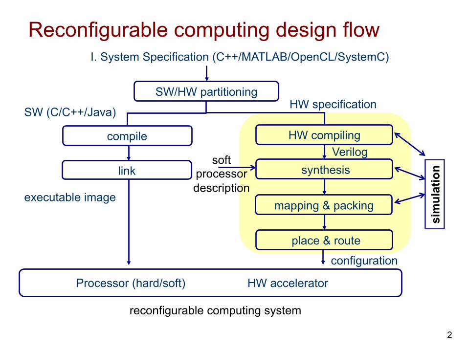
Reconfigurable computing design flow
SW/HW partitioning
SW (C/C++/Java)
I. System Specification (C++/MATLAB/OpenCL/SystemC)
HW specification
HW compiling Verilog
synthesis
mapping & packing
place & route
Processor (hard/soft)
compile
link
configuration
executable image
reconfigurable computing system
HW accelerator
soft processor description
2
sim
ulat
ion
System specification Use High-Level Languages (HLLs) (C, C++, Java, MATLAB).
Advantages: § Since systems consist of both SW and HW, then we can
describe the entire system with the same specification § Fast to code, debug and verify the system is working
Disadvantages: § No concurrent support § No notion of time (clock or delay) § Different communication model than HW (uses signals) § Missing data types (e.g., bit vectors, logic values)
Ø Augment the HLL (e.g. C++) with a new data types, classes, library, to support additional hardware-like functionality (e.g. SystemC)
3
Topics discussed 1. SW/HW partitioning 2. Compilation 3. Synthesis 4. Mapping 5. Packing 6. Placement 7. Routing 8. Simulation 9. Configuration
4
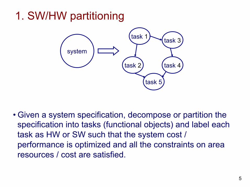
1. SW/HW partitioning
• Given a system specification, decompose or partition the specification into tasks (functional objects) and label each task as HW or SW such that the system cost / performance is optimized and all the constraints on area resources / cost are satisfied.
5
system
task 1
task 2 task 4
task 3
task 5
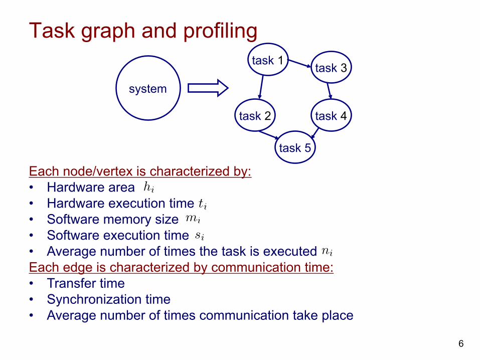
Task graph and profiling
system
Each node/vertex is characterized by: • Hardware area • Hardware execution time • Software memory size • Software execution time • Average number of times the task is executed Each edge is characterized by communication time: • Transfer time • Synchronization time • Average number of times communication take place
task 1
task 2 task 4
task 3
task 5
hi
timi
si
ni
6
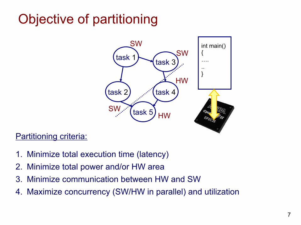
Objective of partitioning
Partitioning criteria:
1. Minimize total execution time (latency) 2. Minimize total power and/or HW area 3. Minimize communication between HW and SW 4. Maximize concurrency (SW/HW in parallel) and utilization
task 1
task 2 task 4
task 3
task 5
int main() { …. .. }
SW
SW HW
HW
SW
7
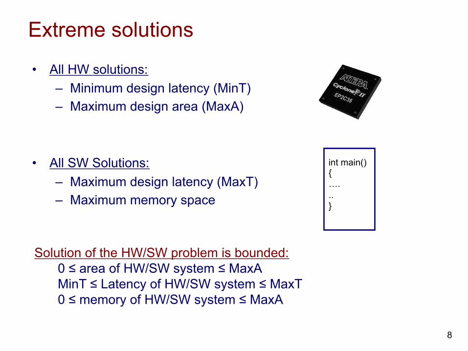
Extreme solutions
• All HW solutions: – Minimum design latency (MinT) – Maximum design area (MaxA)
• All SW Solutions: – Maximum design latency (MaxT) – Maximum memory space
int main() { …. .. }
Solution of the HW/SW problem is bounded: 0 ≤ area of HW/SW system ≤ MaxA MinT ≤ Latency of HW/SW system ≤ MaxT 0 ≤ memory of HW/SW system ≤ MaxA
8
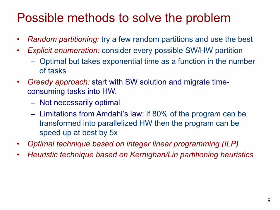
Possible methods to solve the problem • Random partitioning: try a few random partitions and use the best • Explicit enumeration: consider every possible SW/HW partition
– Optimal but takes exponential time as a function in the number of tasks
• Greedy approach: start with SW solution and migrate time-consuming tasks into HW. – Not necessarily optimal – Limitations from Amdahl’s law: if 80% of the program can be
transformed into parallelized HW then the program can be speed up at best by 5x
• Optimal technique based on integer linear programming (ILP) • Heuristic technique based on Kernighan/Lin partitioning heuristics
9
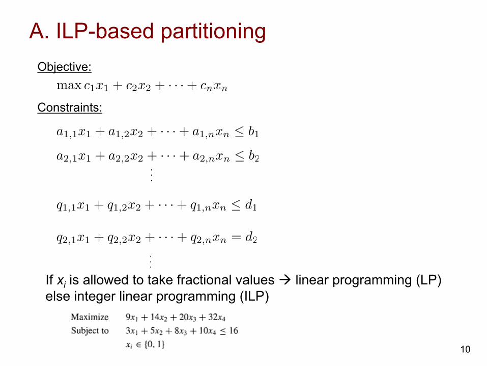
A. ILP-based partitioning Objective:
Constraints:
a2,1x1 + a2,2x2 + · · · + a2,nxn b2
a1,1x1 + a1,2x2 + · · · + a1,nxn b1
q1,1x1 + q1,2x2 + · · · + q1,nxn d1
q2,1x1 + q2,2x2 + · · · + q2,nxn = d2
...
...
max c1x1 + c2x2 + · · · + cnxn
If xi is allowed to take fractional values à linear programming (LP) else integer linear programming (ILP)
10
Examples of LP
• How to solve LP? • What is the runtime? • Many toolboxes are available
[from M. Pinedo]
1 2 3 4 5 6 x1
1
2
3
4
5
6 x2
)objective(6xx 21 =+
4xx2 21 ≤+
12x4x3 21 ≤+
)2,1j(0x12x4x34xx2:tosubjectxxmax
j
21
21
21
=≥
≤+
≤+
+
0
solution space
11
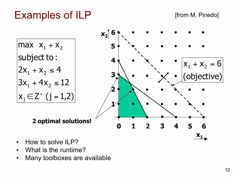
Examples of ILP
• How to solve ILP? • What is the runtime? • Many toolboxes are available
[from M. Pinedo]
1 2 3 4 5 6 x1
1
2
3
4
5
6 x2
)objective(6xx 21 =+
)2,1j(Zx
12x4x34xx2:tosubjectxxmax
j
21
21
21
=∈
≤+
≤+
+
+
0 2 optimal solutions!
12
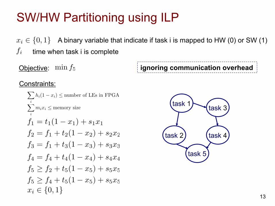
SW/HW Partitioning using ILP
xi 2 {0, 1} A binary variable that indicate if task i is mapped to HW (0) or SW (1)
Objective:
X
i
hi(1� xi) number of LEs in FPGA
X
i
mixi memory size
Constraints:
xi 2 {0, 1}
task 1
task 2 task 4
task 3
task 5
fi time when task i is complete
min f5
f1 = t1(1� x1) + s1x1
f2 = f1 + t2(1� x2) + s2x2
f3 = f1 + t3(1� x3) + s3x3
f4 = f4 + t4(1� x4) + s4x4
f5 � f2 + t5(1� x5) + s5x5
f5 � f4 + t5(1� x5) + s5x5
13
ignoring communication overhead

B. Heuristic approach Total size is constrained by number and size of available FPGA(s)
SW tasks HW tasks
task
task task
task task Execution time
moves
local optimal
global optimal
Kernighan/Lin – Fidducia/Mattheyses algorithm • Start with all task vertices free to swap/move (unlocked) • Label each possible swap/move with immediate change in execution time that
it causes (gain) • Iteratively select and execute a swap/move with highest gain (whether
positive or negative); lock the moving vertex (i.e., cannot move again during the pass),
• Best solution seen during the pass is adopted as starting solution for next pass
14
task
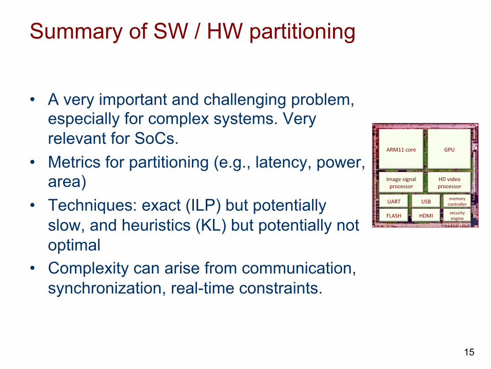
Summary of SW / HW partitioning
• A very important and challenging problem, especially for complex systems. Very relevant for SoCs.
• Metrics for partitioning (e.g., latency, power, area)
• Techniques: exact (ILP) but potentially slow, and heuristics (KL) but potentially not optimal
• Complexity can arise from communication, synchronization, real-time constraints.
15
ARM11%core%
Image%signal%processor%
GPU%
HD%video%processor%
UART% USB%
FLASH%
memory%controller%
security%engine%HDMI%
2. Compilation
• Reconfigurable configurable has the ability to execute multiple operations in parallel through spatial distribution of the computing resources
• We have already studied how HDLs (e.g., Verilog) are synthesized to logic
• High-level algorithmic descriptions lack descriptions of concurrency. When compiling an algorithmic description or SW-based language into HW, it is necessary to expose the concurrency in the application. How can we do that?
16
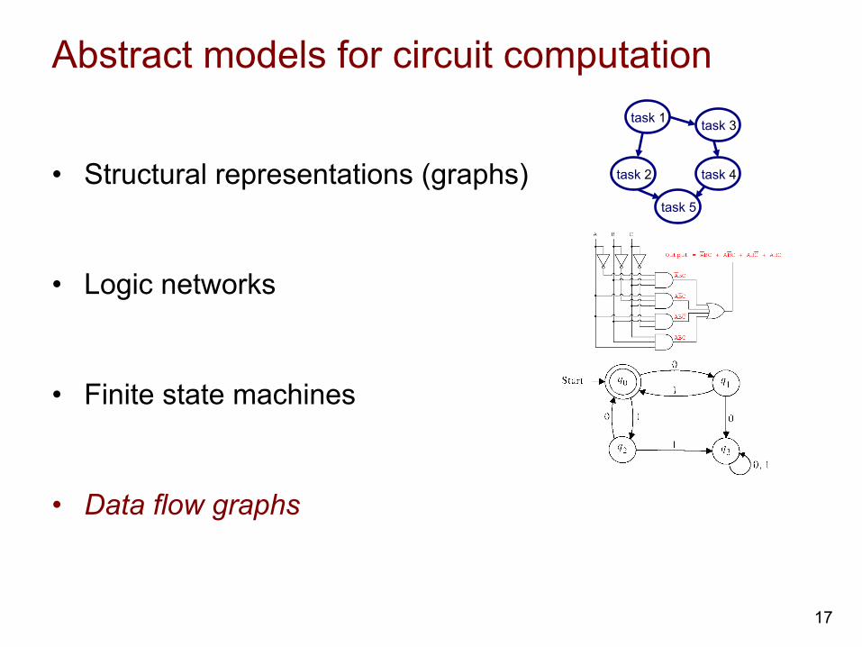
Abstract models for circuit computation
• Structural representations (graphs)
• Logic networks
• Finite state machines
• Data flow graphs
17
task 1
task 2 task 4
task 3
task 5
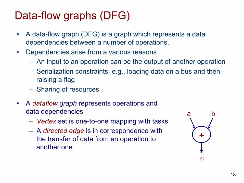
Data-flow graphs (DFG) • A data-flow graph (DFG) is a graph which represents a data
dependencies between a number of operations. • Dependencies arise from a various reasons
– An input to an operation can be the output of another operation – Serialization constraints, e.g., loading data on a bus and then
raising a flag – Sharing of resources
• A dataflow graph represents operations and data dependencies – Vertex set is one-to-one mapping with tasks – A directed edge is in correspondence with
the transfer of data from an operation to another one
+
a b
c
18
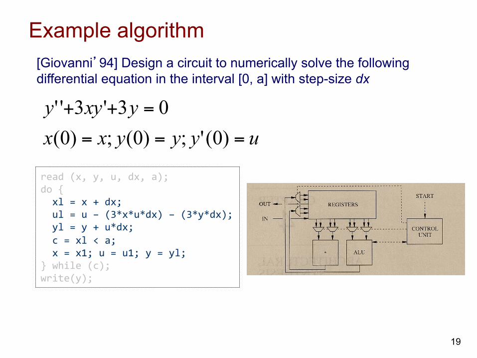
Example algorithm
uyyyxxyxyy
===
=++
)0(';)0(;)0(03'3''
[Giovanni’94] Design a circuit to numerically solve the following differential equation in the interval [0, a] with step-size dx
read (x, y, u, dx, a); do { xl = x + dx; ul = u – (3*x*u*dx) – (3*y*dx); yl = y + u*dx; c = xl < a; x = x1; u = u1; y = yl; } while (c); write(y);
19

DFG of algorithm xl = x + dx; ul = u – (3*x*u*dx) – (3*y*dx); yl = y + u*dx; c = xl < a;
* *
*
-
*
*
-
* +
3 x u dx 3 y u dx dx x
+ <
a
xl y
dx
yl c u
u1 20
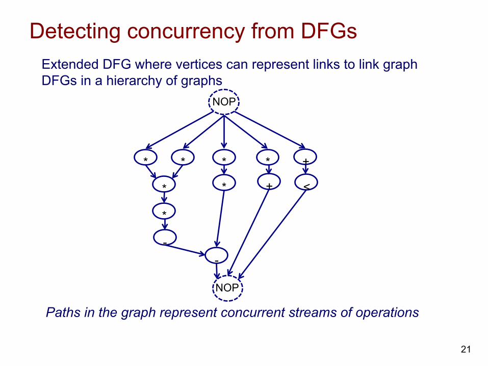
Detecting concurrency from DFGs
* *
*
*
-
*
*
-
* +
+ <
Paths in the graph represent concurrent streams of operations
Extended DFG where vertices can represent links to link graph DFGs in a hierarchy of graphs
NOP
NOP
21
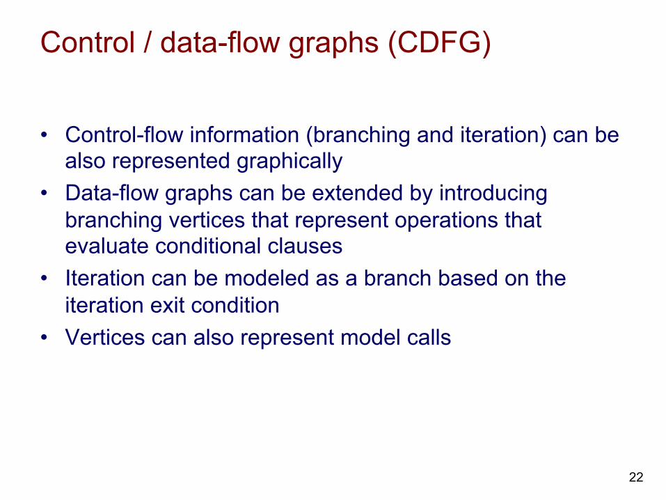
Control / data-flow graphs (CDFG)
• Control-flow information (branching and iteration) can be also represented graphically
• Data-flow graphs can be extended by introducing branching vertices that represent operations that evaluate conditional clauses
• Iteration can be modeled as a branch based on the iteration exit condition
• Vertices can also represent model calls
22
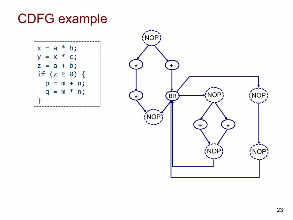
CDFG example
x = a * b; y = x * c; z = a + b; if (z ≥ 0) { p = m + n; q = m * n; }
NOP
*
*
NOP
BR
+
NOP
+ *
NOP
NOP
NOP
23
Code transformations
24
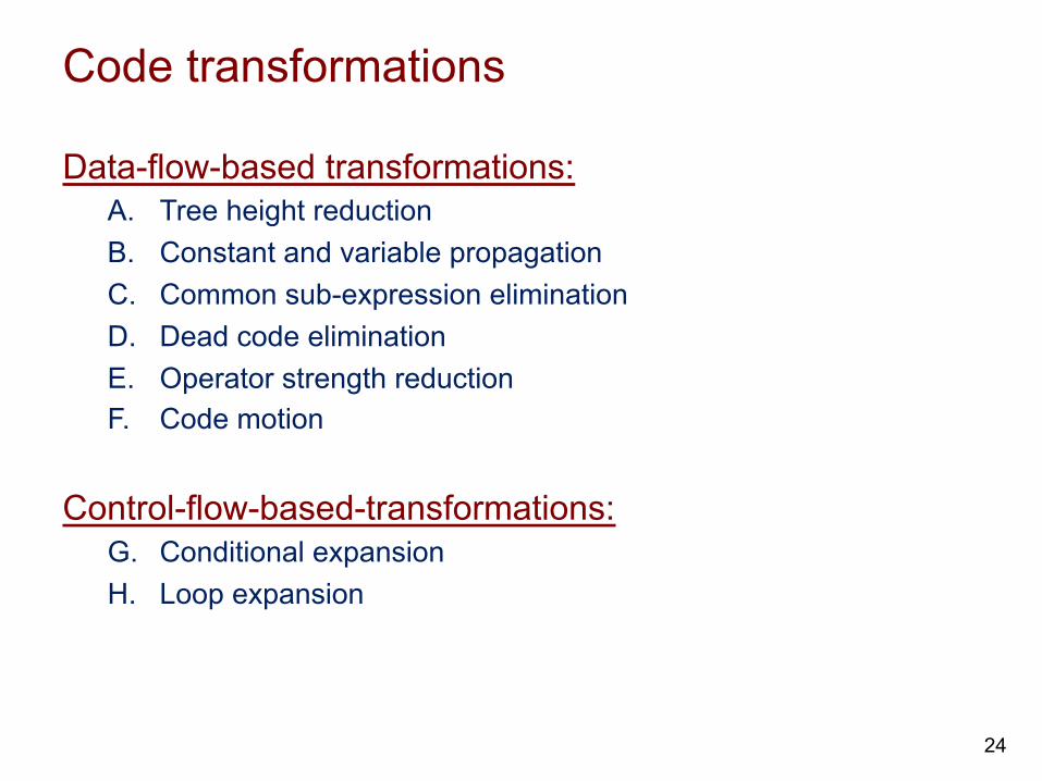
Data-flow-based transformations: A. Tree height reduction B. Constant and variable propagation C. Common sub-expression elimination D. Dead code elimination E. Operator strength reduction F. Code motion
Control-flow-based-transformations: G. Conditional expansion H. Loop expansion
A. Tree-height reduction (THR)
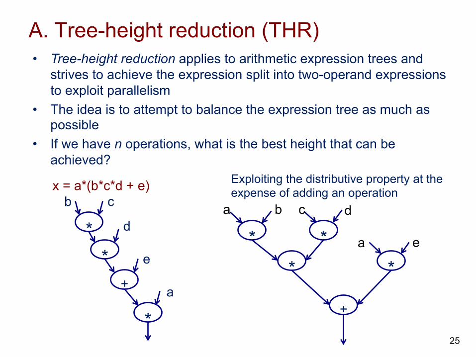
x = a*(b*c*d + e)
+
* *
*
b c
d
e
a
* * a b c d
* * a e
+
Exploiting the distributive property at the expense of adding an operation
25
• Tree-height reduction applies to arithmetic expression trees and strives to achieve the expression split into two-operand expressions to exploit parallelism
• The idea is to attempt to balance the expression tree as much as possible
• If we have n operations, what is the best height that can be achieved?

A. Impact of serializing memory accesses on tree height reduction
26
original after serialization after THR after THR & serialization
[example from Cardoso ‘10]
• Bandwidth to the memory is critical to realize the speed-up potential of reconfigurable systems
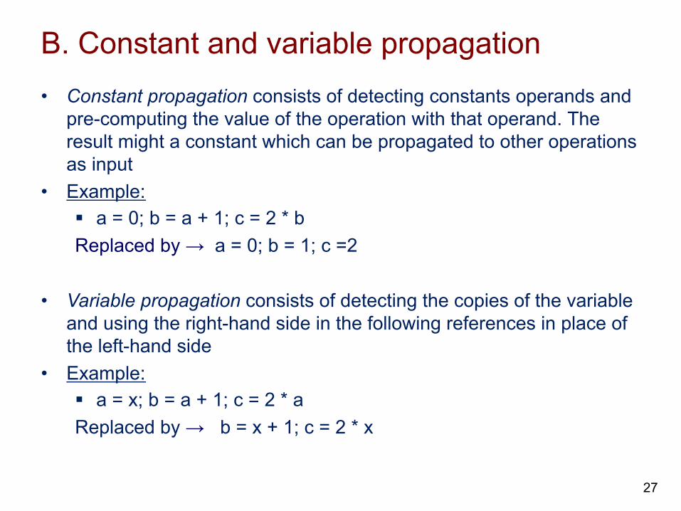
B. Constant and variable propagation • Constant propagation consists of detecting constants operands and
pre-computing the value of the operation with that operand. The result might a constant which can be propagated to other operations as input
• Example: § a = 0; b = a + 1; c = 2 * b Replaced by → a = 0; b = 1; c =2
• Variable propagation consists of detecting the copies of the variable and using the right-hand side in the following references in place of the left-hand side
• Example: § a = x; b = a + 1; c = 2 * a Replaced by → b = x + 1; c = 2 * x
27
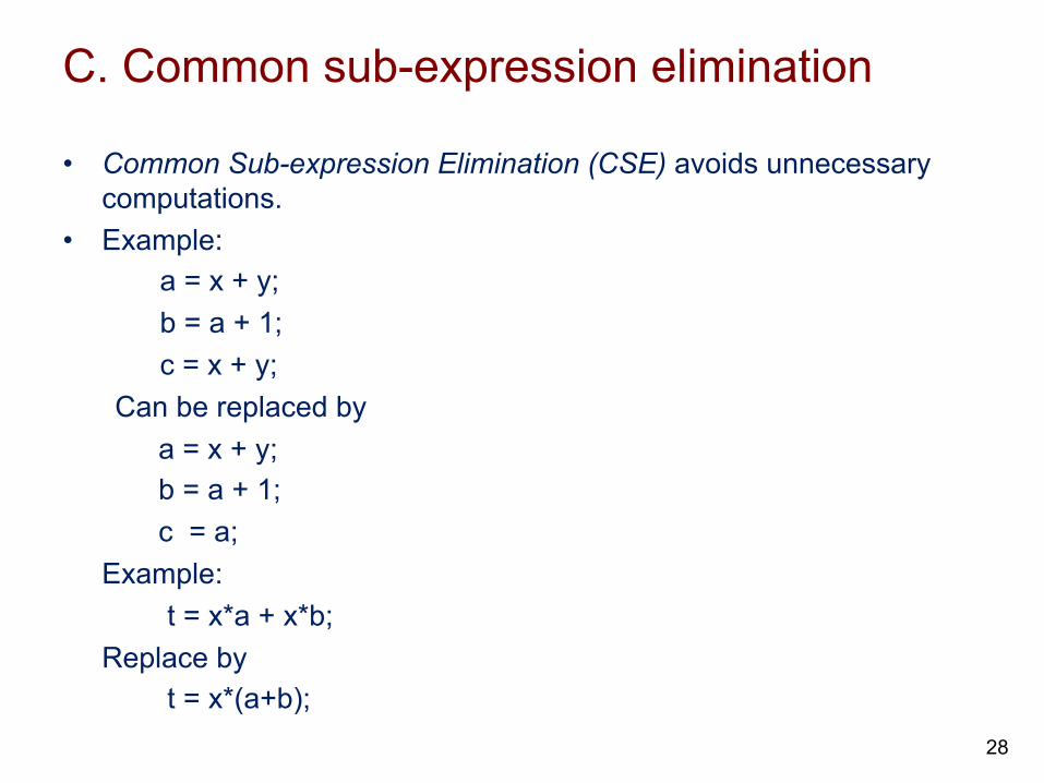
C. Common sub-expression elimination
• Common Sub-expression Elimination (CSE) avoids unnecessary computations.
• Example: a = x + y; b = a + 1; c = x + y;
Can be replaced by a = x + y; b = a + 1; c = a;
Example: t = x*a + x*b;
Replace by t = x*(a+b);
28
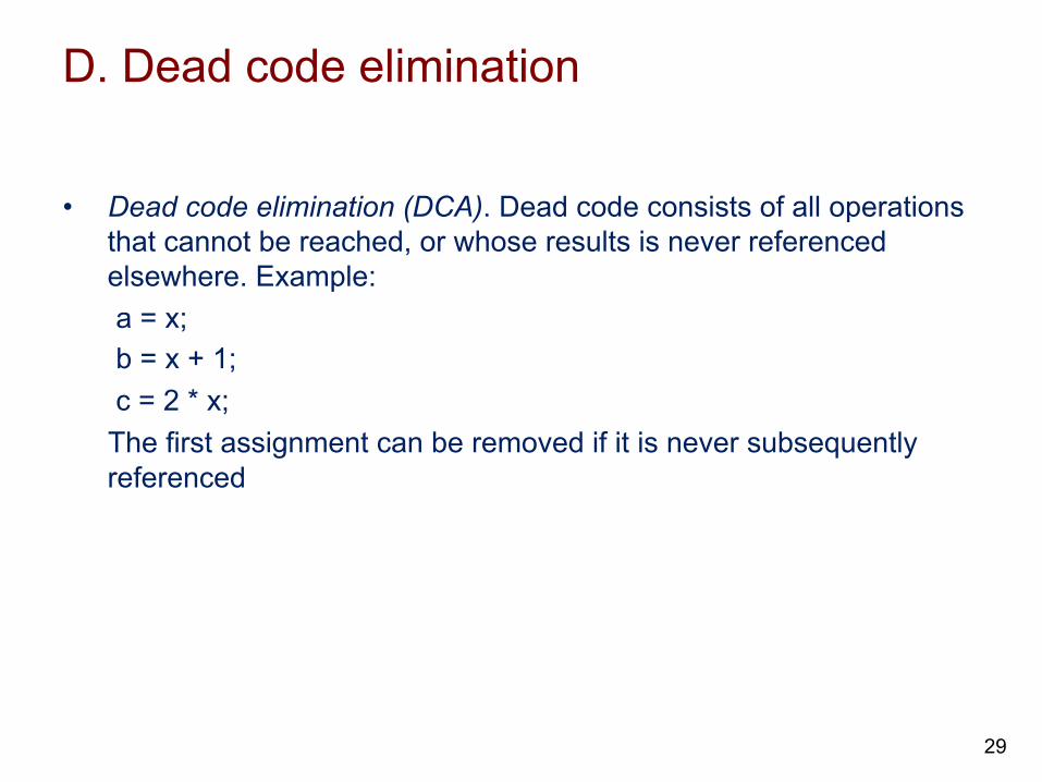
D. Dead code elimination
• Dead code elimination (DCA). Dead code consists of all operations that cannot be reached, or whose results is never referenced elsewhere. Example: a = x; b = x + 1; c = 2 * x; The first assignment can be removed if it is never subsequently referenced
29
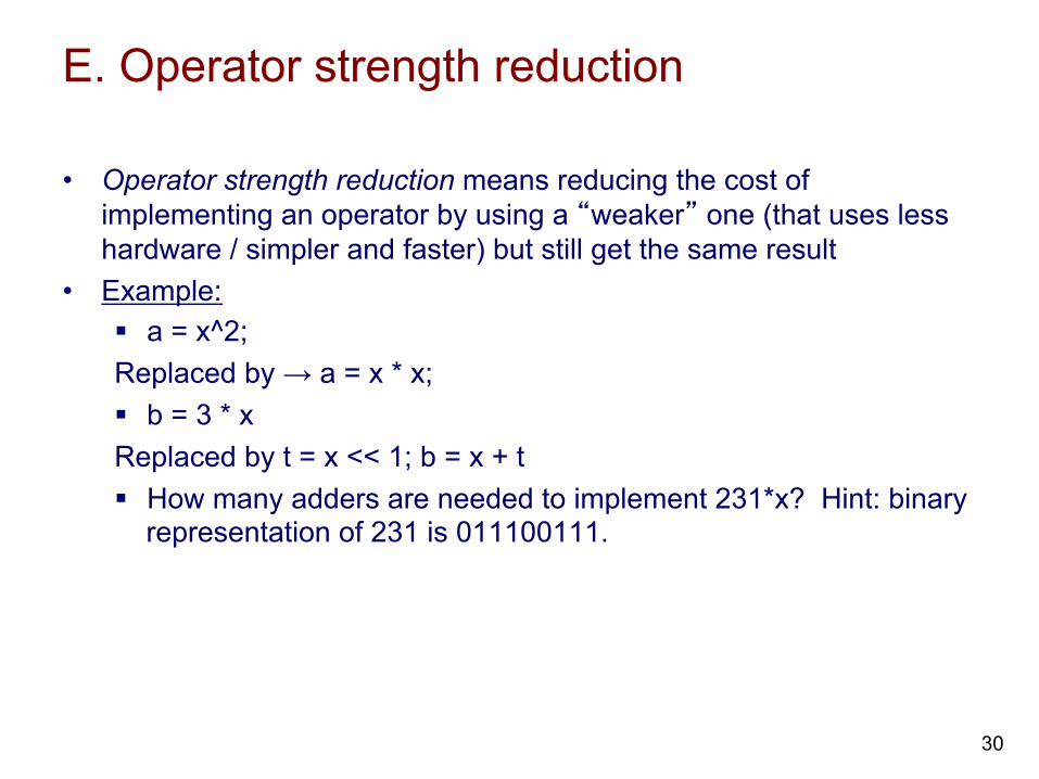
E. Operator strength reduction
• Operator strength reduction means reducing the cost of implementing an operator by using a “weaker” one (that uses less hardware / simpler and faster) but still get the same result
• Example: § a = x^2; Replaced by → a = x * x; § b = 3 * x Replaced by t = x << 1; b = x + t § How many adders are needed to implement 231*x? Hint: binary
representation of 231 is 011100111.
30

F. Code motion: hoisting and sinking
31
• Code motion (up – hoisting or down – sinking) may have the potential benefit of making the two computations independent, thus enabling concurrent execution. Such movement may increase the potential for other optimization techniques.
• Examples: 1. for (i = 1; i < a *b) {…} Replaced by → t = a * b; for ( i =1; i <= t) {…} 2. before code hoisting after code hoisting
[example from Cardoso ‘10]
G. Conditional expansion
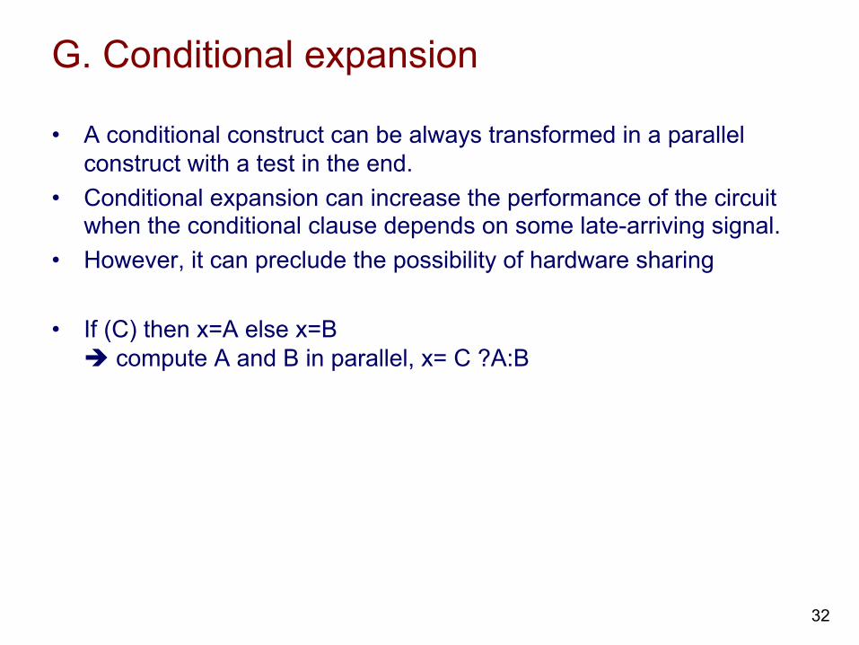
• A conditional construct can be always transformed in a parallel construct with a test in the end.
• Conditional expansion can increase the performance of the circuit when the conditional clause depends on some late-arriving signal.
• However, it can preclude the possibility of hardware sharing
• If (C) then x=A else x=B è compute A and B in parallel, x= C ?A:B
32
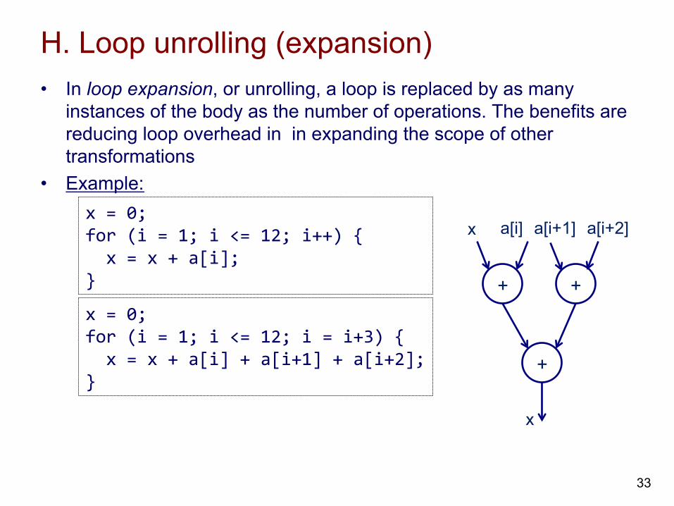
H. Loop unrolling (expansion) • In loop expansion, or unrolling, a loop is replaced by as many
instances of the body as the number of operations. The benefits are reducing loop overhead in in expanding the scope of other transformations
• Example: x = 0; for (i = 1; i <= 12; i++) { x = x + a[i]; }
x = 0; for (i = 1; i <= 12; i = i+3) { x = x + a[i] + a[i+1] + a[i+2]; }
+
+
+
x a[i] a[i+1]
x
a[i+2]
33
Data oriented transformations
34
A. Bit-width narrowing and bit optimizations B. Data distribution C. Data replication D. Scalar replacement E. Data transformation for floating points
A. Bit width optimizations
35
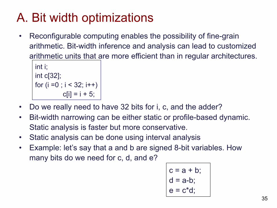
• Reconfigurable computing enables the possibility of fine-grain arithmetic. Bit-width inference and analysis can lead to customized arithmetic units that are more efficient than in regular architectures.
• Do we really need to have 32 bits for i, c, and the adder? • Bit-width narrowing can be either static or profile-based dynamic.
Static analysis is faster but more conservative. • Static analysis can be done using interval analysis • Example: let’s say that a and b are signed 8-bit variables. How
many bits do we need for c, d, and e?
int i; int c[32]; for (i =0 ; i < 32; i++)
c[i] = i + 5;
c = a + b; d = a-b; e = c*d;
B. Data distribution
36
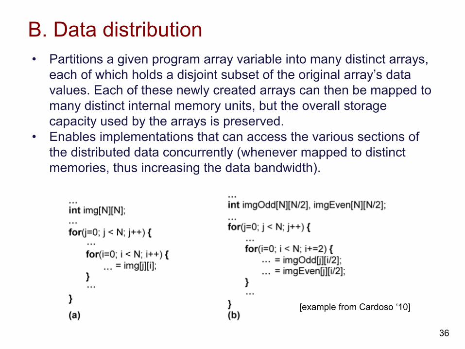
• Partitions a given program array variable into many distinct arrays, each of which holds a disjoint subset of the original array’s data values. Each of these newly created arrays can then be mapped to many distinct internal memory units, but the overall storage capacity used by the arrays is preserved.
• Enables implementations that can access the various sections of the distributed data concurrently (whenever mapped to distinct memories, thus increasing the data bandwidth).
[example from Cardoso ‘10]
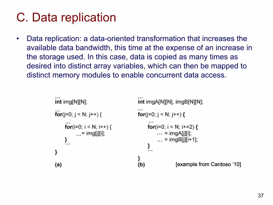
C. Data replication
37
• Data replication: a data-oriented transformation that increases the available data bandwidth, this time at the expense of an increase in the storage used. In this case, data is copied as many times as desired into distinct array variables, which can then be mapped to distinct memory modules to enable concurrent data access.
[example from Cardoso ‘10] [example from Cardoso ‘10]
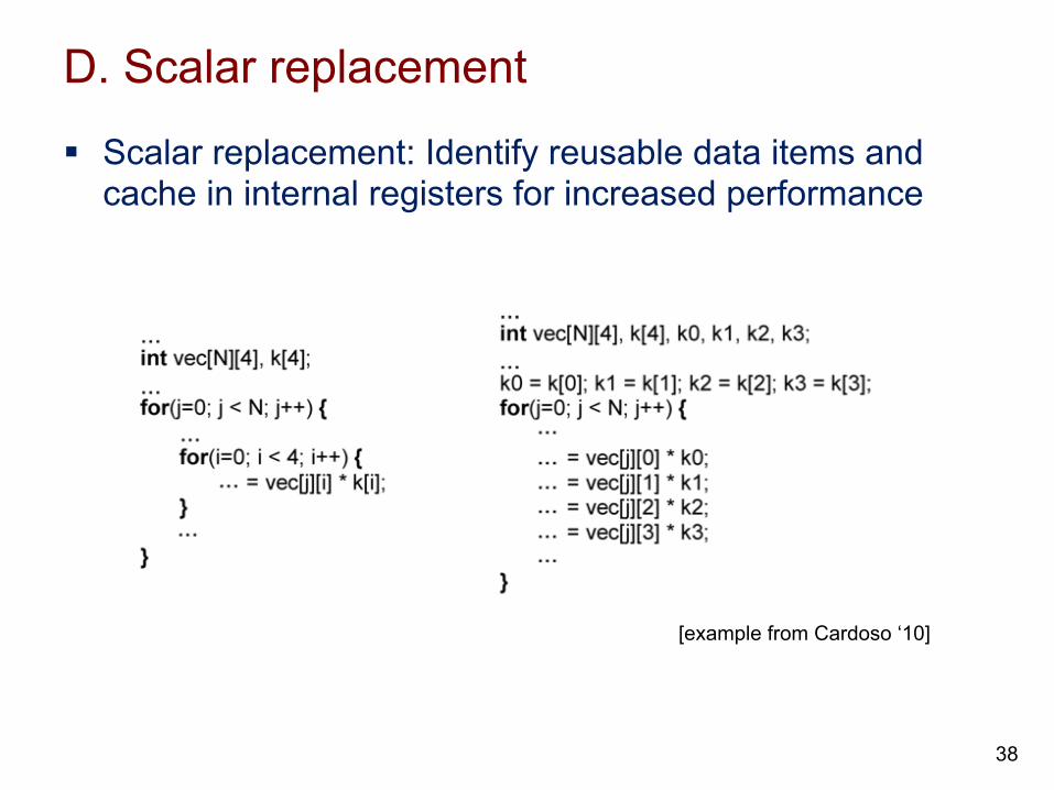
D. Scalar replacement
38
§ Scalar replacement: Identify reusable data items and cache in internal registers for increased performance
[example from Cardoso ‘10]
E. Data transformations for floating points
39
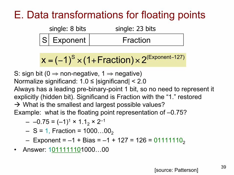
S: sign bit (0 ⇒ non-negative, 1 ⇒ negative) Normalize significand: 1.0 ≤ |significand| < 2.0 Always has a leading pre-binary-point 1 bit, so no need to represent it explicitly (hidden bit). Significand is Fraction with the “1.” restored à What is the smallest and largest possible values? Example: what is the floating point representation of –0.75?
– –0.75 = (–1)1 × 1.12 × 2–1
– S = 1, Fraction = 1000…002 – Exponent = –1 + Bias = –1 + 127 = 126 = 011111102
• Answer: 1011111101000…00
S Exponent Fraction single: 8 bits single: 23 bits
x = (−1)S × (1+Fraction)×2(Exponent−127)
[source: Patterson]
E. Example of floating point addition
40
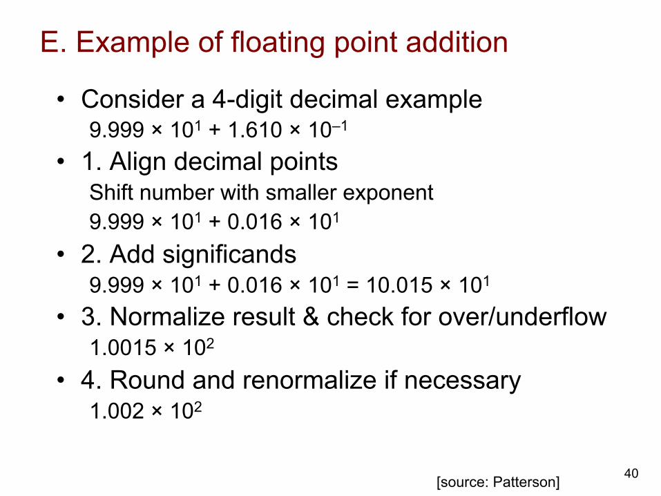
• Consider a 4-digit decimal example 9.999 × 101 + 1.610 × 10⁻¹
• 1. Align decimal points Shift number with smaller exponent 9.999 × 101 + 0.016 × 101
• 2. Add significands 9.999 × 101 + 0.016 × 101 = 10.015 × 101
• 3. Normalize result & check for over/underflow 1.0015 × 10²
• 4. Round and renormalize if necessary 1.002 × 10²
[source: Patterson]
E. Example of floating point addition
41
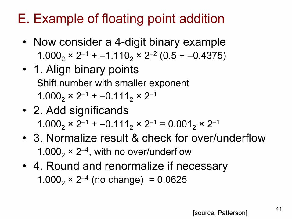
• Now consider a 4-digit binary example 1.0002 × 2–1 + –1.1102 × 2–2 (0.5 + –0.4375)
• 1. Align binary points Shift number with smaller exponent 1.0002 × 2–1 + –0.1112 × 2–1
• 2. Add significands 1.0002 × 2–1 + –0.1112 × 2–1 = 0.0012 × 2–1
• 3. Normalize result & check for over/underflow 1.0002 × 2–4, with no over/underflow
• 4. Round and renormalize if necessary 1.0002 × 2–4 (no change) = 0.0625
[source: Patterson]
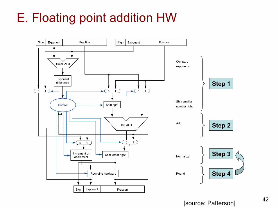
E. Floating point addition HW
42
Step 1
Step 2
Step 3
Step 4
[source: Patterson]
E. Comparison of HW area requirements
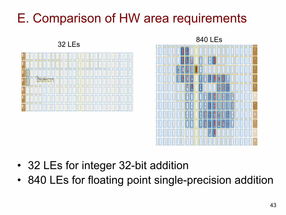
43
• 32 LEs for integer 32-bit addition • 840 LEs for floating point single-precision addition
32 LEs 840 LEs
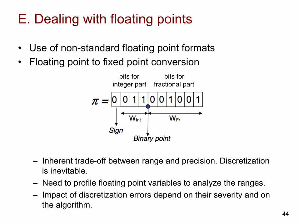
E. Dealing with floating points
• Use of non-standard floating point formats • Floating point to fixed point conversion
– Inherent trade-off between range and precision. Discretization is inevitable.
– Need to profile floating point variables to analyze the ranges. – Impact of discretization errors depend on their severity and on
the algorithm. 44
bits for integer part
bits for fractional part
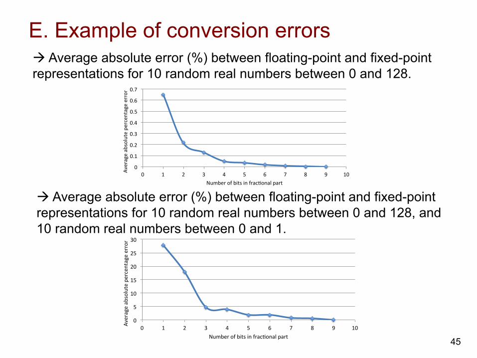
E. Example of conversion errors
45
0"
5"
10"
15"
20"
25"
30"
0" 1" 2" 3" 4" 5" 6" 7" 8" 9" 10"Average"absolute"percentage"error"
Number"of"bits"in"frac?onal"part"
0"
0.1"
0.2"
0.3"
0.4"
0.5"
0.6"
0.7"
0" 1" 2" 3" 4" 5" 6" 7" 8" 9" 10"Average"absolute"percentage"error"
Number"of"bits"in"frac@onal"part"
à Average absolute error (%) between floating-point and fixed-point representations for 10 random real numbers between 0 and 128.
à Average absolute error (%) between floating-point and fixed-point representations for 10 random real numbers between 0 and 128, and 10 random real numbers between 0 and 1.
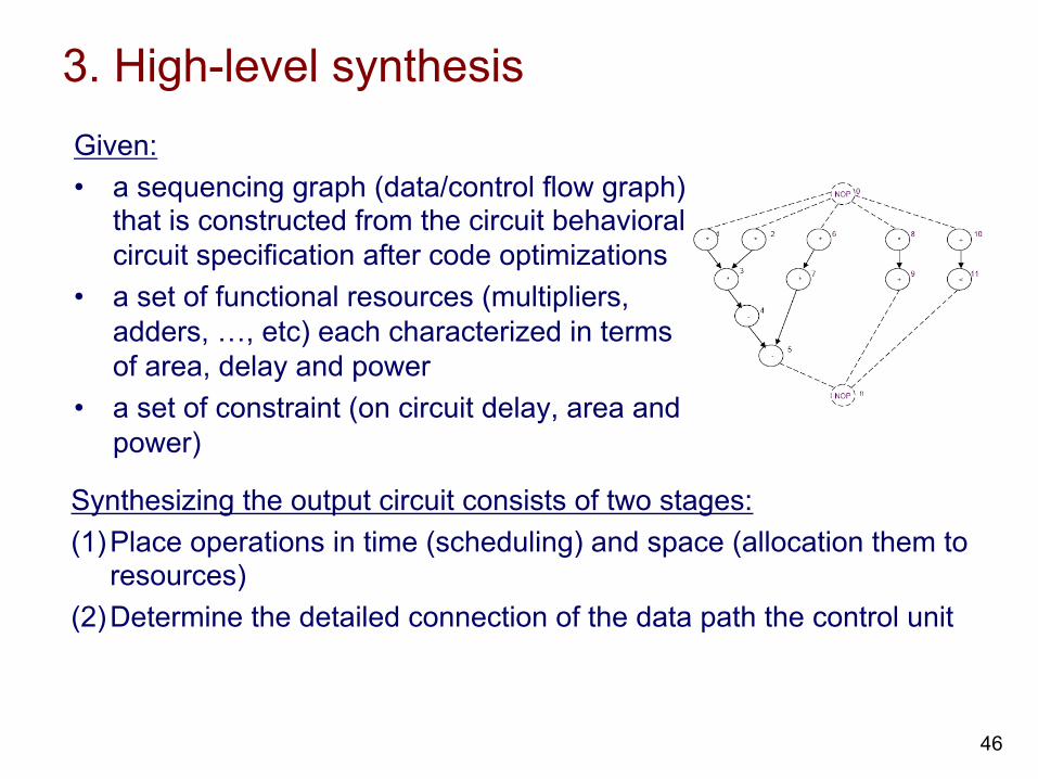
3. High-level synthesis Given: • a sequencing graph (data/control flow graph)
that is constructed from the circuit behavioral circuit specification after code optimizations
• a set of functional resources (multipliers, adders, …, etc) each characterized in terms of area, delay and power
• a set of constraint (on circuit delay, area and power)
Synthesizing the output circuit consists of two stages: (1) Place operations in time (scheduling) and space (allocation them to
resources) (2) Determine the detailed connection of the data path the control unit
46
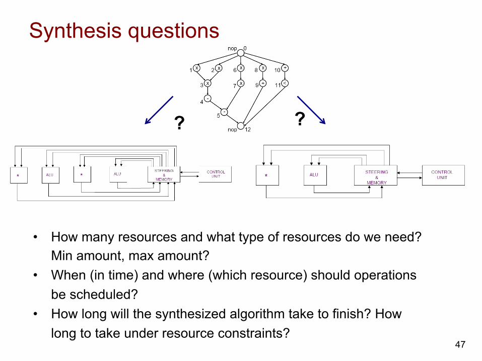
Synthesis questions
47
? ?
• How many resources and what type of resources do we need? Min amount, max amount?
• When (in time) and where (which resource) should operations be scheduled?
• How long will the synthesized algorithm take to finish? How long to take under resource constraints?
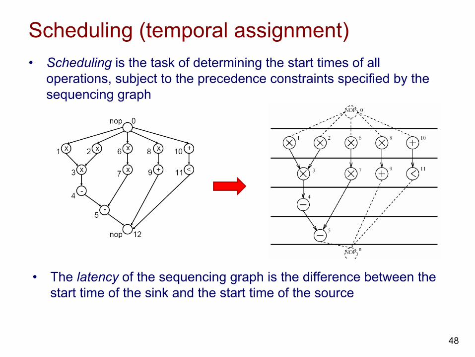
Scheduling (temporal assignment) • Scheduling is the task of determining the start times of all
operations, subject to the precedence constraints specified by the sequencing graph
• The latency of the sequencing graph is the difference between the start time of the sink and the start time of the source
48
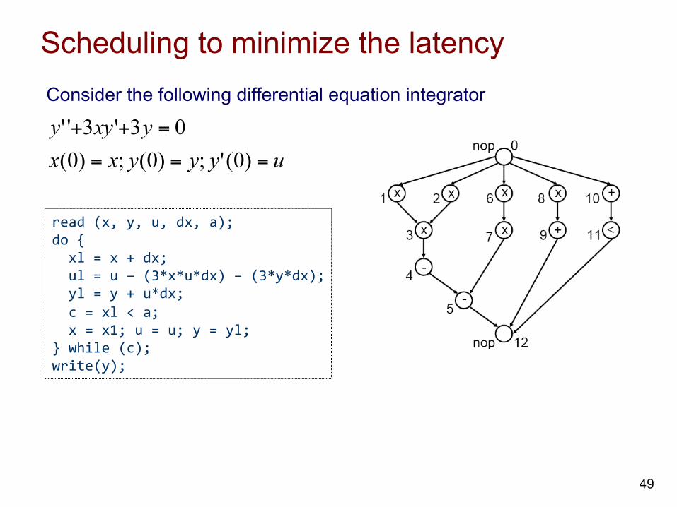
Scheduling to minimize the latency
uyyyxxyxyy
===
=++
)0(';)0(;)0(03'3''
read (x, y, u, dx, a); do { xl = x + dx; ul = u – (3*x*u*dx) – (3*y*dx); yl = y + u*dx; c = xl < a; x = x1; u = u; y = yl; } while (c); write(y);
Consider the following differential equation integrator
49
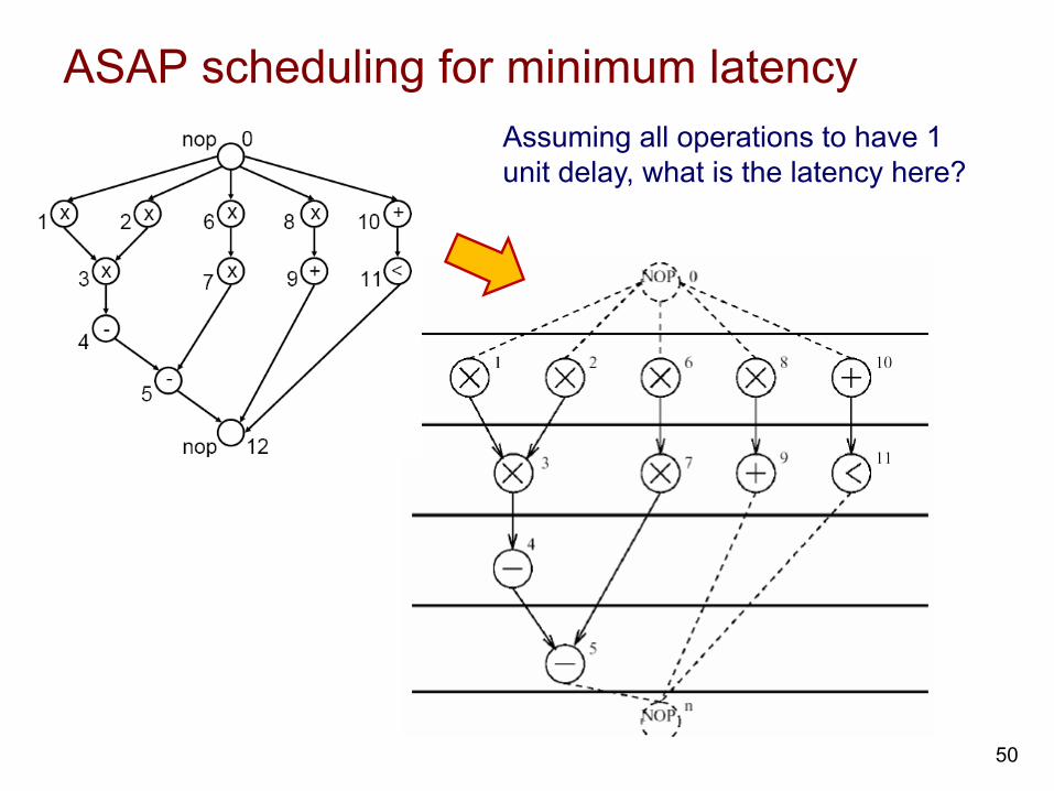
ASAP scheduling for minimum latency Assuming all operations to have 1 unit delay, what is the latency here?
50
ASAP scheduling algorithm
51
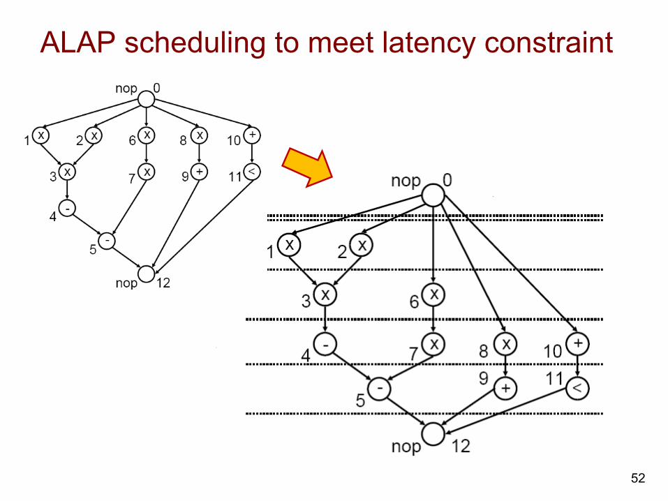
ALAP scheduling to meet latency constraint
52
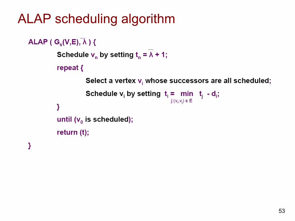
ALAP scheduling algorithm
53
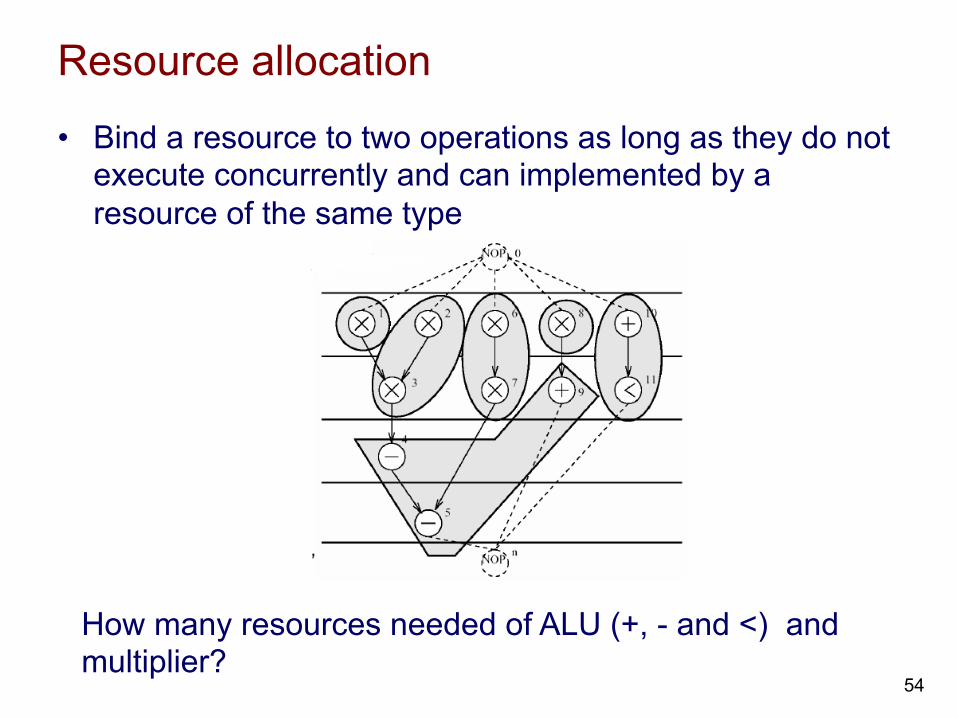
Resource allocation
• Bind a resource to two operations as long as they do not execute concurrently and can implemented by a resource of the same type
How many resources needed of ALU (+, - and <) and multiplier?
54
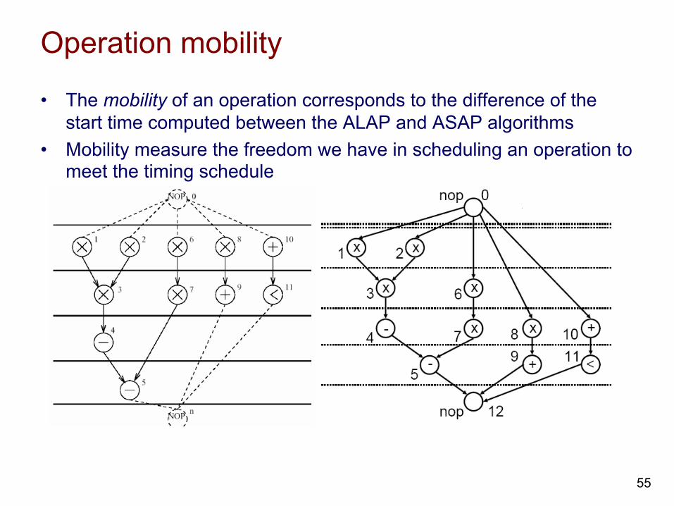
Operation mobility
• The mobility of an operation corresponds to the difference of the start time computed between the ALAP and ASAP algorithms
• Mobility measure the freedom we have in scheduling an operation to meet the timing schedule
55
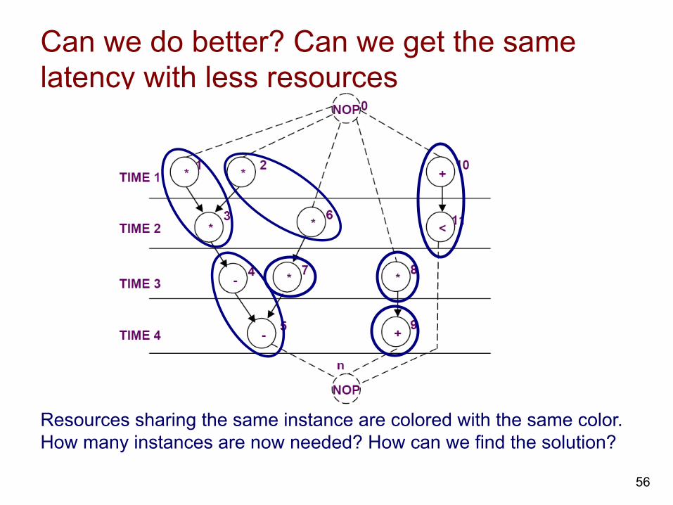
Can we do better? Can we get the same latency with less resources
Resources sharing the same instance are colored with the same color. How many instances are now needed? How can we find the solution?
56
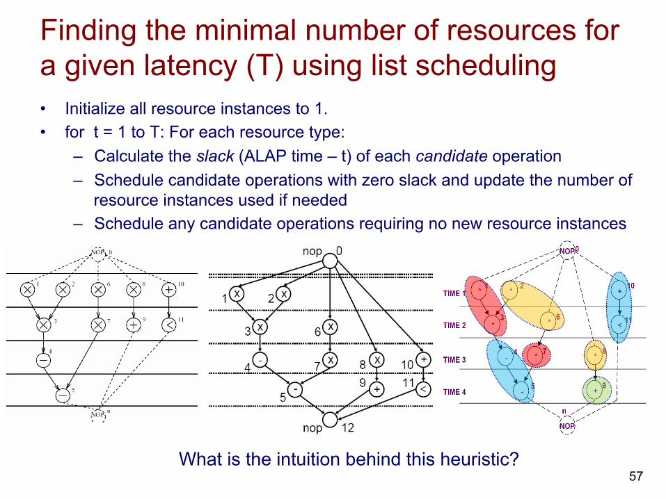
Finding the minimal number of resources for a given latency (T) using list scheduling • Initialize all resource instances to 1. • for t = 1 to T: For each resource type:
– Calculate the slack (ALAP time – t) of each candidate operation – Schedule candidate operations with zero slack and update the number of
resource instances used if needed – Schedule any candidate operations requiring no new resource instances
What is the intuition behind this heuristic? 57
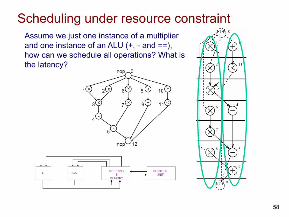
Scheduling under resource constraint Assume we just one instance of a multiplier and one instance of an ALU (+, - and ==), how can we schedule all operations? What is the latency?
58
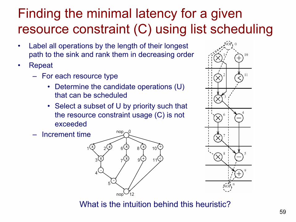
Finding the minimal latency for a given resource constraint (C) using list scheduling • Label all operations by the length of their longest
path to the sink and rank them in decreasing order • Repeat
– For each resource type • Determine the candidate operations (U)
that can be scheduled • Select a subset of U by priority such that
the resource constraint usage (C) is not exceeded
– Increment time
What is the intuition behind this heuristic? 59
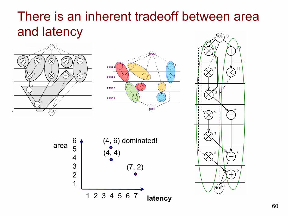
There is an inherent tradeoff between area and latency
latency
area (4, 6) dominated!
(7, 2)
(4, 4)
1 2 3 4 5 6 7
6 5 4 3 2 1
60
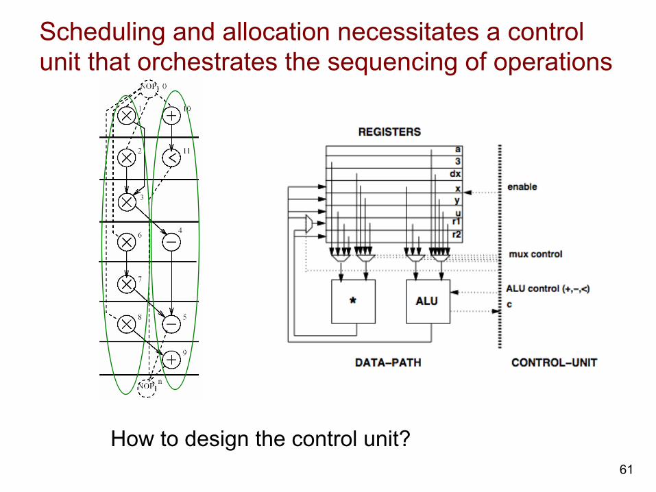
Scheduling and allocation necessitates a control unit that orchestrates the sequencing of operations
61
How to design the control unit?

Control unit example for(i=0; i<10; i=i+1) begin x = a[i] + b[i]; z = z + x; end
a
b
x
z
i Control
unit
CMP
10
Enable
+
MUX MUX
1
How many control signals are produced from the control unit? How can we design the control unit?
101001 111001
.
.
.
counter control
bits
62
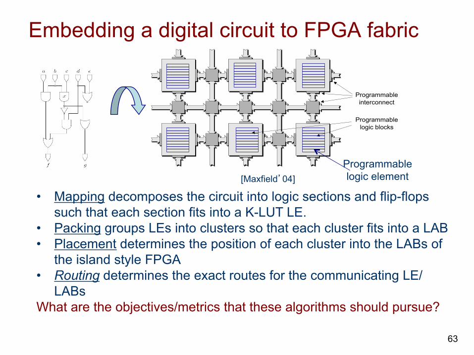
Embedding a digital circuit to FPGA fabric
Programmableinterconnect
Programmablelogic blocks
[Maxfield’04] Programmable logic element
• Mapping decomposes the circuit into logic sections and flip-flops such that each section fits into a K-LUT LE.
• Packing groups LEs into clusters so that each cluster fits into a LAB • Placement determines the position of each cluster into the LABs of
the island style FPGA • Routing determines the exact routes for the communicating LE/
LABs What are the objectives/metrics that these algorithms should pursue?
63
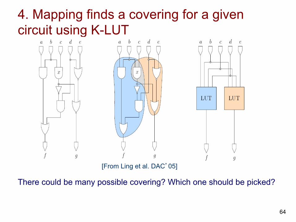
4. Mapping finds a covering for a given circuit using K-LUT
[From Ling et al. DAC’05]
There could be many possible covering? Which one should be picked?
64
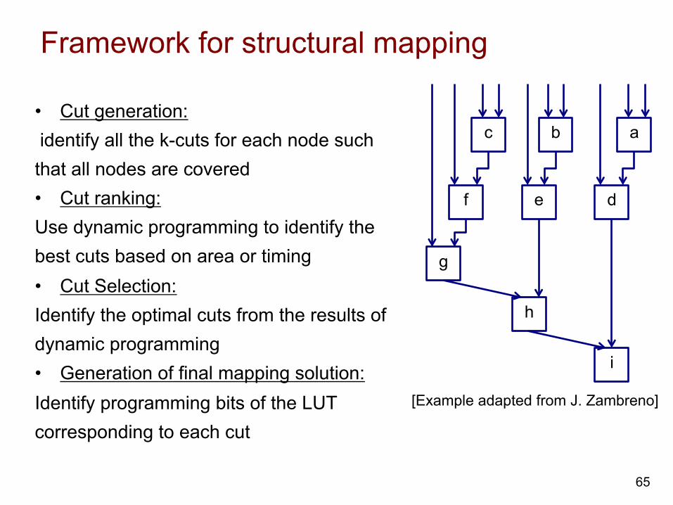
Framework for structural mapping
65
c b a
f e d
g
h
i
[Example adapted from J. Zambreno]
• Cut generation: identify all the k-cuts for each node such that all nodes are covered • Cut ranking: Use dynamic programming to identify the best cuts based on area or timing • Cut Selection: Identify the optimal cuts from the results of dynamic programming • Generation of final mapping solution: Identify programming bits of the LUT corresponding to each cut
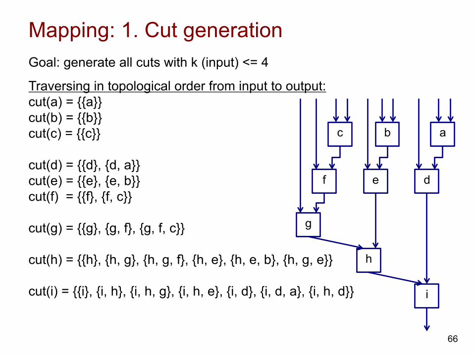
Mapping: 1. Cut generation
66
c b a
f e d
g
h
i
Goal: generate all cuts with k (input) <= 4
Traversing in topological order from input to output: cut(a) = {{a}} cut(b) = {{b}} cut(c) = {{c}} cut(d) = {{d}, {d, a}} cut(e) = {{e}, {e, b}} cut(f) = {{f}, {f, c}} cut(g) = {{g}, {g, f}, {g, f, c}} cut(h) = {{h}, {h, g}, {h, g, f}, {h, e}, {h, e, b}, {h, g, e}} cut(i) = {{i}, {i, h}, {i, h, g}, {i, h, e}, {i, d}, {i, d, a}, {i, h, d}}
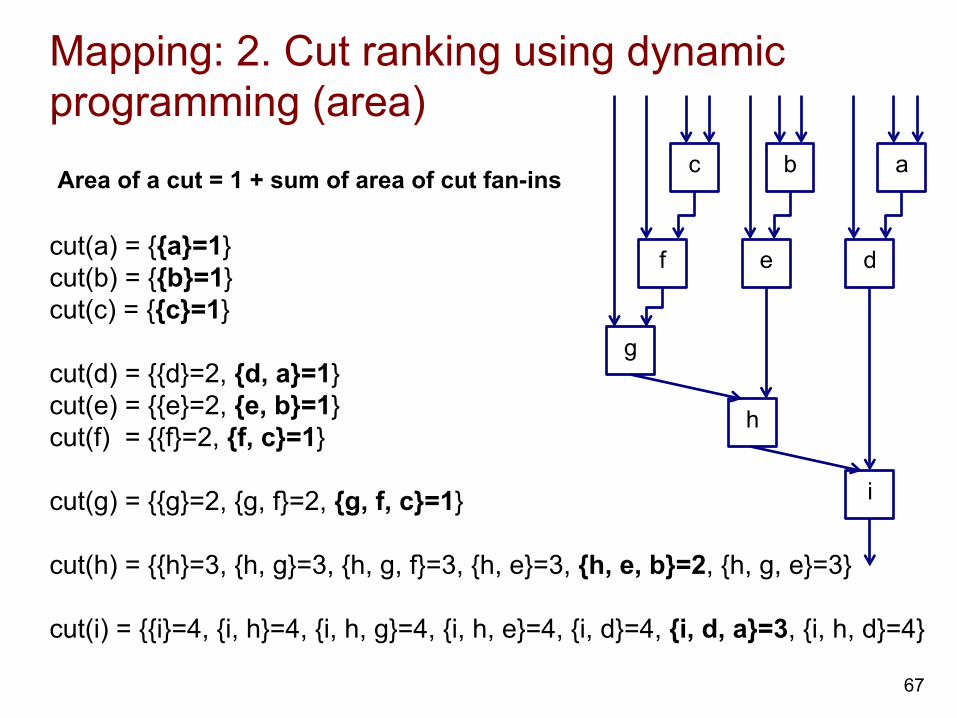
Mapping: 2. Cut ranking using dynamic programming (area)
67
c b a
f e d
g
h
i
cut(a) = {{a}=1} cut(b) = {{b}=1} cut(c) = {{c}=1} cut(d) = {{d}=2, {d, a}=1} cut(e) = {{e}=2, {e, b}=1} cut(f) = {{f}=2, {f, c}=1} cut(g) = {{g}=2, {g, f}=2, {g, f, c}=1} cut(h) = {{h}=3, {h, g}=3, {h, g, f}=3, {h, e}=3, {h, e, b}=2, {h, g, e}=3} cut(i) = {{i}=4, {i, h}=4, {i, h, g}=4, {i, h, e}=4, {i, d}=4, {i, d, a}=3, {i, h, d}=4}
Area of a cut = 1 + sum of area of cut fan-ins
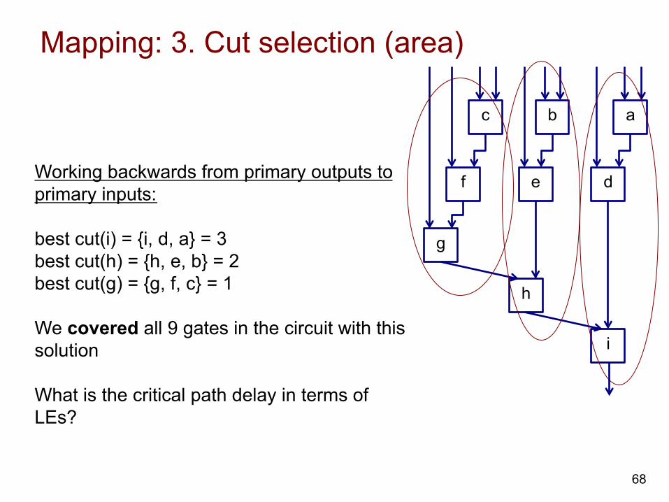
Mapping: 3. Cut selection (area)
68
c b a
f e d
g
h
i
Working backwards from primary outputs to primary inputs: best cut(i) = {i, d, a} = 3 best cut(h) = {h, e, b} = 2 best cut(g) = {g, f, c} = 1 We covered all 9 gates in the circuit with this solution What is the critical path delay in terms of LEs?
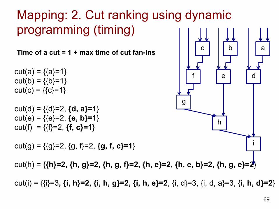
Mapping: 2. Cut ranking using dynamic programming (timing)
69
c b a
f e d
g
h
i
cut(a) = {{a}=1} cut(b) = {{b}=1} cut(c) = {{c}=1} cut(d) = {{d}=2, {d, a}=1} cut(e) = {{e}=2, {e, b}=1} cut(f) = {{f}=2, {f, c}=1} cut(g) = {{g}=2, {g, f}=2, {g, f, c}=1} cut(h) = {{h}=2, {h, g}=2, {h, g, f}=2, {h, e}=2, {h, e, b}=2, {h, g, e}=2} cut(i) = {{i}=3, {i, h}=2, {i, h, g}=2, {i, h, e}=2, {i, d}=3, {i, d, a}=3, {i, h, d}=2}
Time of a cut = 1 + max time of cut fan-ins
Mapping: 3. Cut selection (timing)
70
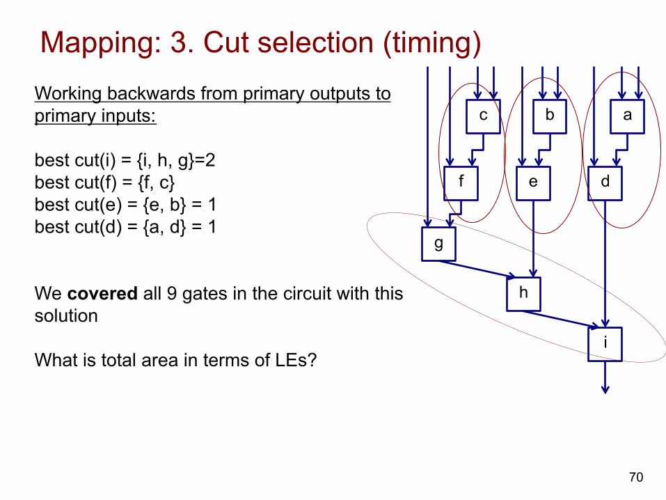
Working backwards from primary outputs to primary inputs: best cut(i) = {i, h, g}=2 best cut(f) = {f, c} best cut(e) = {e, b} = 1 best cut(d) = {a, d} = 1 We covered all 9 gates in the circuit with this solution What is total area in terms of LEs?
c b a
f e d
g
h
i
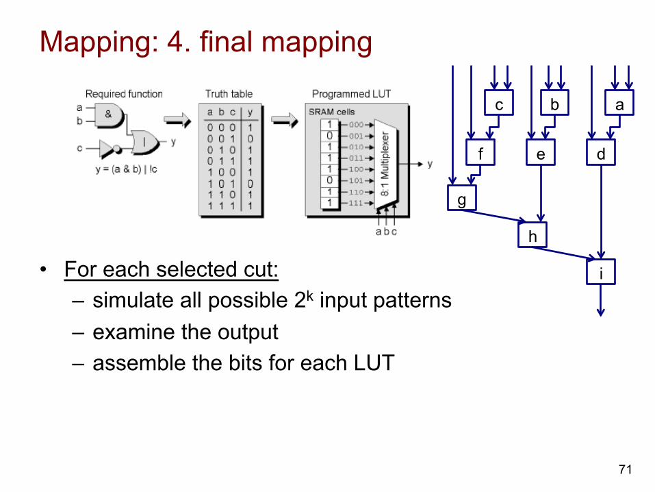
Mapping: 4. final mapping
• For each selected cut: – simulate all possible 2k input patterns – examine the output – assemble the bits for each LUT
71
c b a
f e d
g
h
i
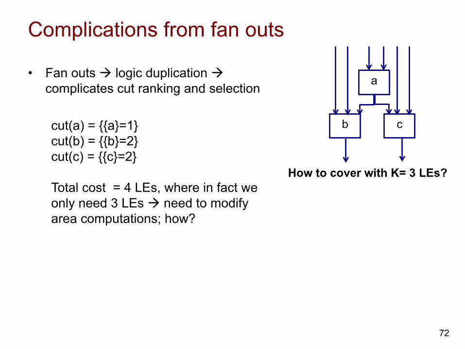
Complications from fan outs
• Fan outs à logic duplication à complicates cut ranking and selection
72
a
c b
How to cover with K= 3 LEs?
cut(a) = {{a}=1} cut(b) = {{b}=2} cut(c) = {{c}=2} Total cost = 4 LEs, where in fact we only need 3 LEs à need to modify area computations; how?
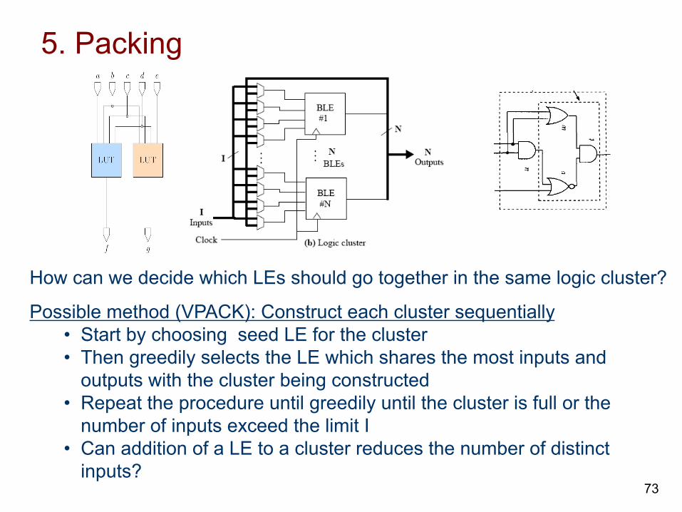
5. Packing
How can we decide which LEs should go together in the same logic cluster?
Possible method (VPACK): Construct each cluster sequentially • Start by choosing seed LE for the cluster • Then greedily selects the LE which shares the most inputs and
outputs with the cluster being constructed • Repeat the procedure until greedily until the cluster is full or the
number of inputs exceed the limit I • Can addition of a LE to a cluster reduces the number of distinct
inputs? 73
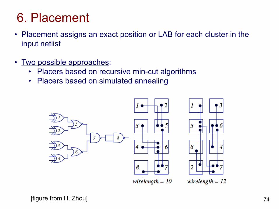
6. Placement • Placement assigns an exact position or LAB for each cluster in the
input netlist
• Two possible approaches: • Placers based on recursive min-cut algorithms • Placers based on simulated annealing
74 [figure from H. Zhou]

How to measure wire length for nets with fanout > 1?
75
1. Semi-perimeter method: Half the perimeter of the bounding rectangle that encloses all the pins of the net to be connected. Most widely used approximation!
2. Complete graph: Since #edges in a complete graph (n(n−1))/2
3. Minimum chain: Start from one vertex and connect to the closest one, and then to the next closest, etc.
[slide adapted from H. Zhou]
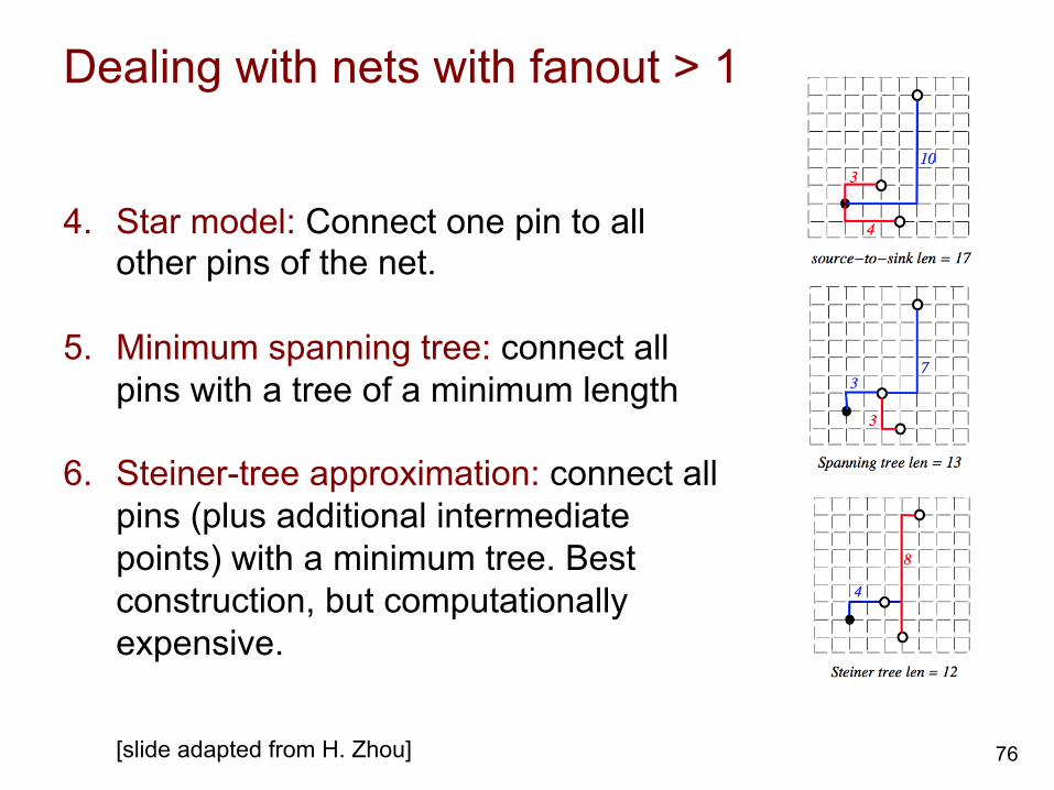
Dealing with nets with fanout > 1
76
4. Star model: Connect one pin to all other pins of the net.
5. Minimum spanning tree: connect all
pins with a tree of a minimum length
6. Steiner-tree approximation: connect all pins (plus additional intermediate points) with a minimum tree. Best construction, but computationally expensive.
[slide adapted from H. Zhou]
77
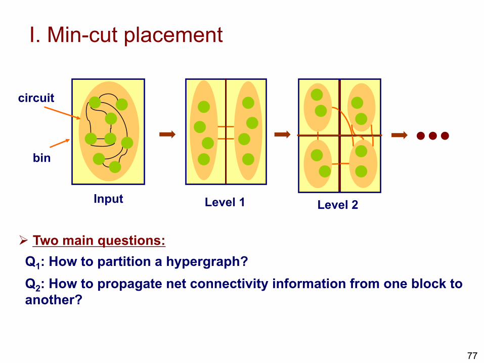
I. Min-cut placement
Input
Ø Two main questions: Q1: How to partition a hypergraph? Q2: How to propagate net connectivity information from one block to another?
circuit
bin
Level 1 Level 2
78
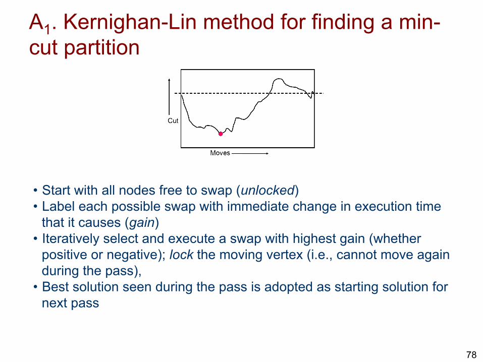
A1. Kernighan-Lin method for finding a min-cut partition
• Start with all nodes free to swap (unlocked) • Label each possible swap with immediate change in execution time
that it causes (gain) • Iteratively select and execute a swap with highest gain (whether
positive or negative); lock the moving vertex (i.e., cannot move again during the pass),
• Best solution seen during the pass is adopted as starting solution for next pass
79
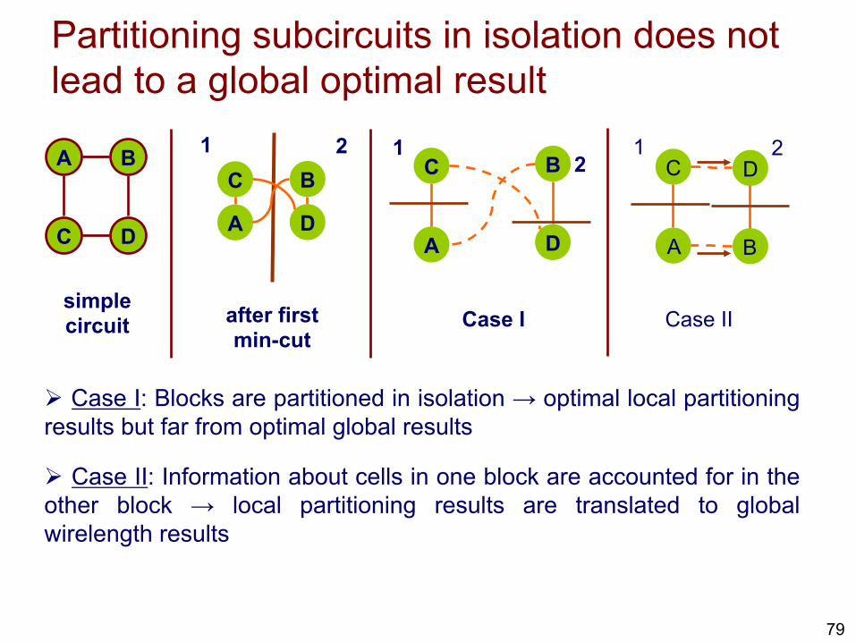
Partitioning subcircuits in isolation does not lead to a global optimal result
A B
C D
simple circuit
A
B C
D
1 2
after first min-cut
Case II
1 2
A B
C D
Ø Case II: Information about cells in one block are accounted for in the other block → local partitioning results are translated to global wirelength results
1 2
A
B C
D
Case I
Ø Case I: Blocks are partitioned in isolation → optimal local partitioning results but far from optimal global results
1

80
A2: Terminal propagation is good technique to capture global connectivity
B1 B2 u
v
uf
Ø B1 has been partitioned; B2 is to be partitioned
Ø u is propagated as a fixed vertex uf to the subblock that is closer
Ø uf biases the partitioner to move v upward
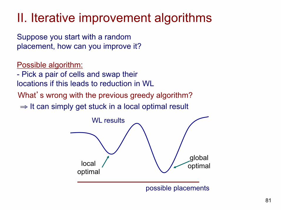
II. Iterative improvement algorithms
81
What’s wrong with the previous greedy algorithm?
Suppose you start with a random placement, how can you improve it? Possible algorithm: - Pick a pair of cells and swap their locations if this leads to reduction in WL
WL results
possible placements
local optimal
global optimal
⇒ It can simply get stuck in a local optimal result
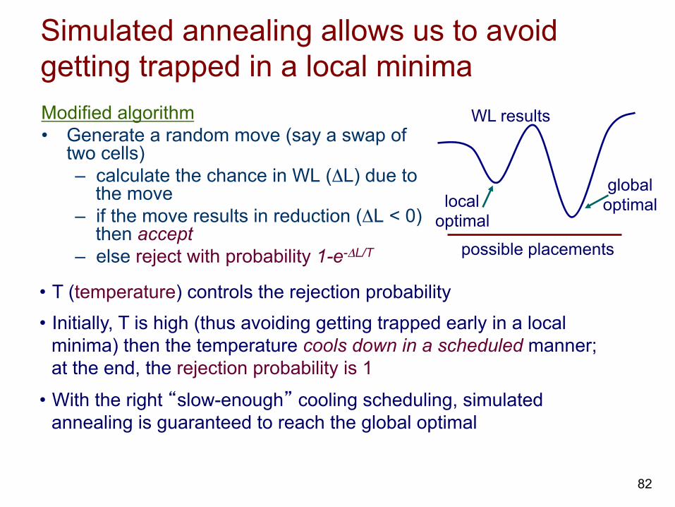
Simulated annealing allows us to avoid getting trapped in a local minima Modified algorithm • Generate a random move (say a swap of
two cells) – calculate the chance in WL (ΔL) due to
the move – if the move results in reduction (ΔL < 0)
then accept – else reject with probability 1-e-ΔL/T
• T (temperature) controls the rejection probability • Initially, T is high (thus avoiding getting trapped early in a local
minima) then the temperature cools down in a scheduled manner; at the end, the rejection probability is 1
• With the right “slow-enough” cooling scheduling, simulated annealing is guaranteed to reach the global optimal
WL results
possible placements
local optimal
global optimal
82
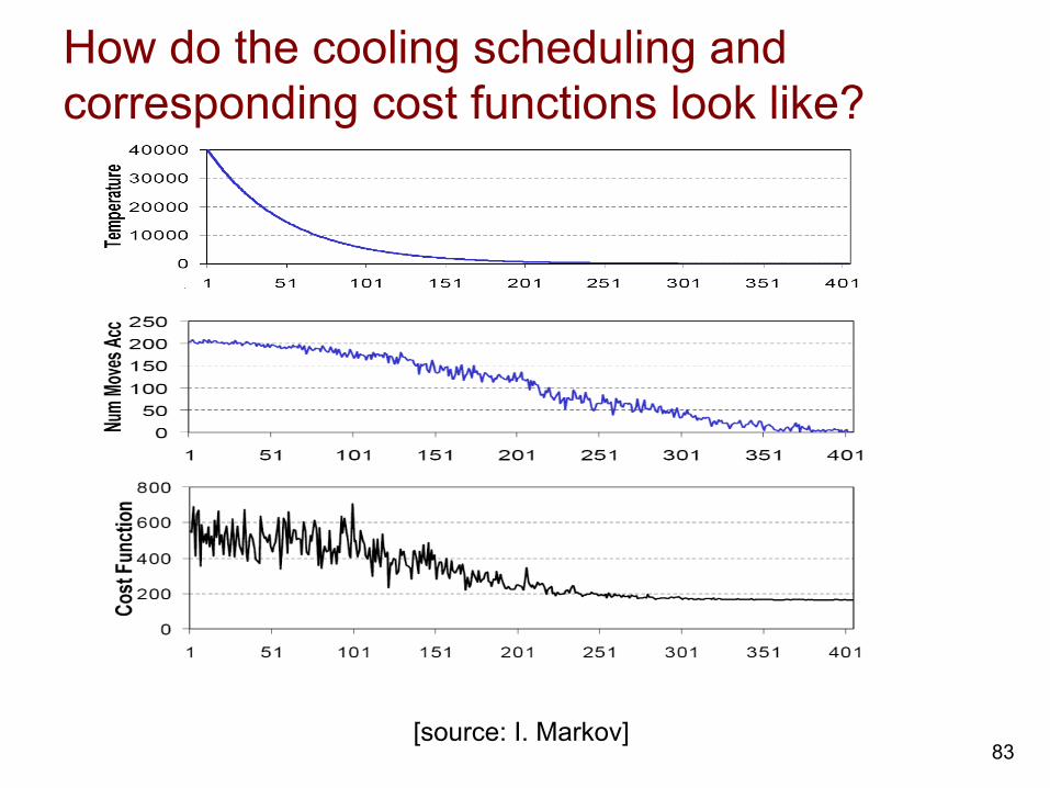
How do the cooling scheduling and corresponding cost functions look like?
[source: I. Markov] 83
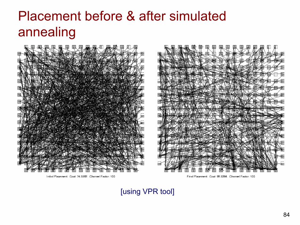
Placement before & after simulated annealing
[using VPR tool]
84
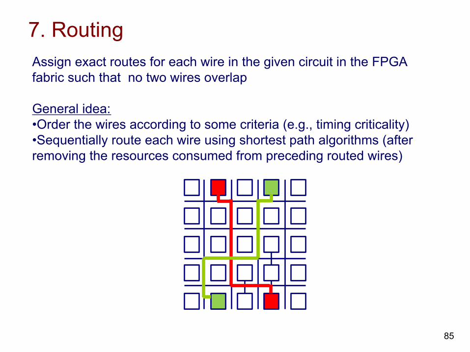
7. Routing Assign exact routes for each wire in the given circuit in the FPGA fabric such that no two wires overlap General idea: • Order the wires according to some criteria (e.g., timing criticality) • Sequentially route each wire using shortest path algorithms (after removing the resources consumed from preceding routed wires)
85
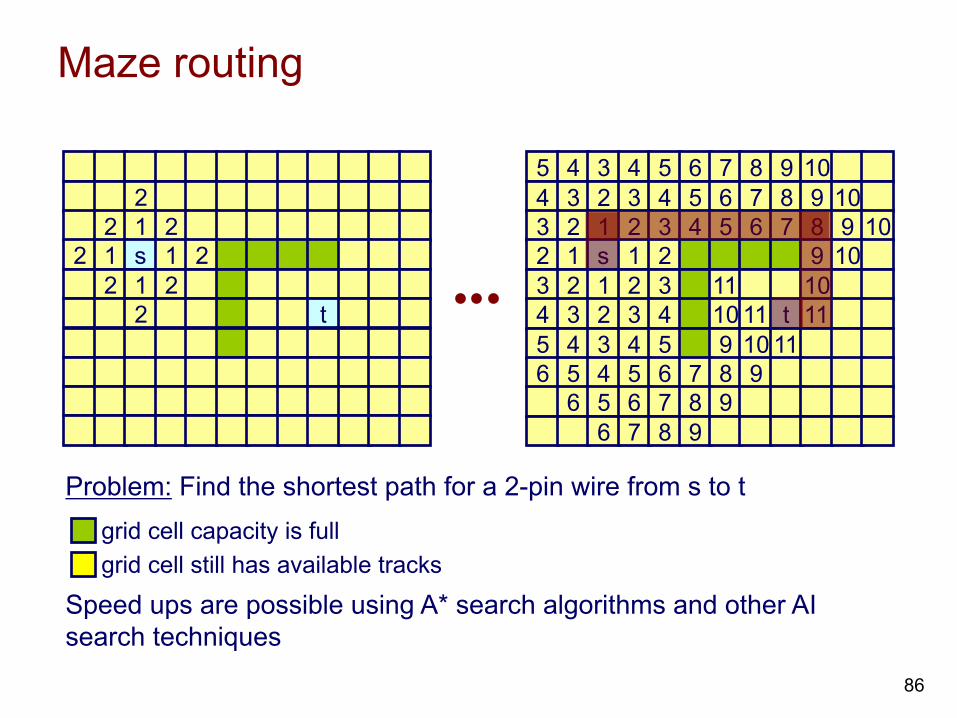
Maze routing
2 2 1 2
2 1 s 1 2 2 1 2
2 t
Problem: Find the shortest path for a 2-pin wire from s to t
5 4 3 4 5 6 7 8 9 10 4 3 2 3 4 5 6 7 8 9 10 3 2 1 2 3 4 5 6 7 8 9 10 2 1 s 1 2 9 10 3 2 1 2 3 11 10 4 3 2 3 4 10 11 t 11 5 4 3 4 5 9 10 11 6 5 4 5 6 7 8 9
6 5 6 7 8 9 6 7 8 9
grid cell capacity is full grid cell still has available tracks
Speed ups are possible using A* search algorithms and other AI search techniques
86
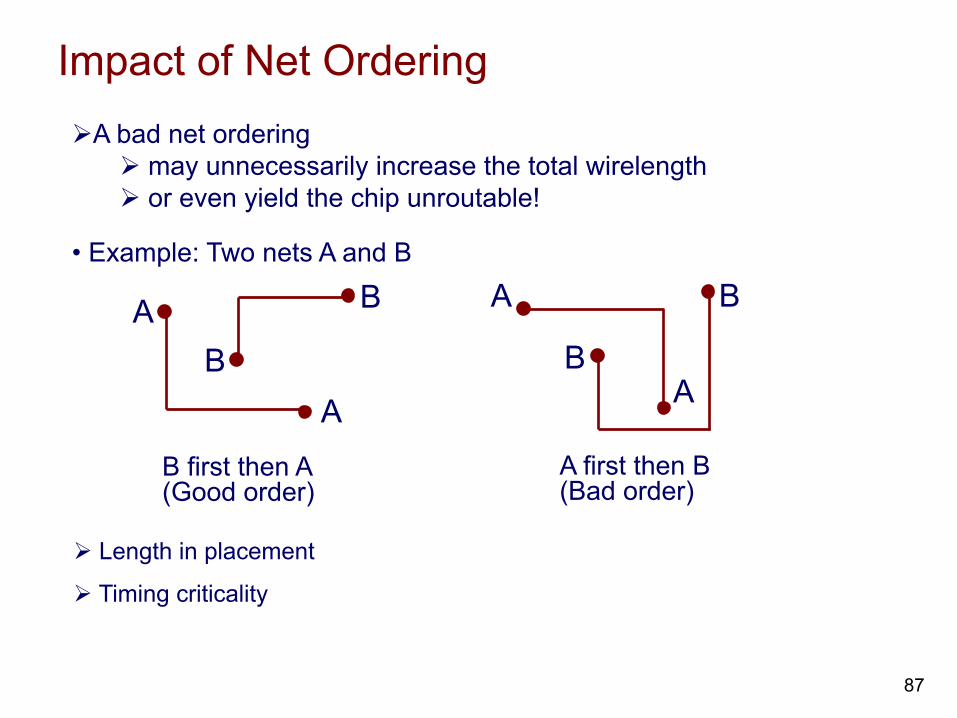
Impact of Net Ordering Ø A bad net ordering
Ø may unnecessarily increase the total wirelength Ø or even yield the chip unroutable!
A
A B
B
B first then A (Good order)
A
A B
B
A first then B (Bad order)
• Example: Two nets A and B
Ø Length in placement
Ø Timing criticality
87
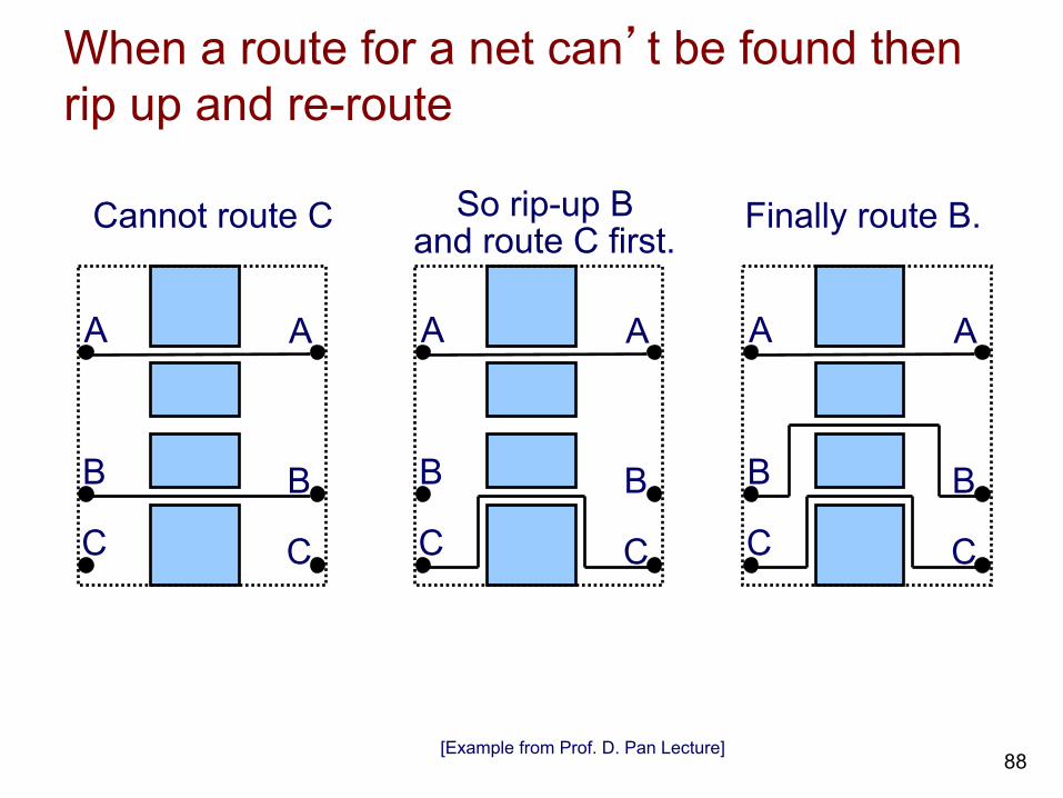
When a route for a net can’t be found then rip up and re-route
A
B
C
A
B
C
Cannot route C
A
B
C
A
B
C
So rip-up B and route C first.
A
B
C
A
B
C
Finally route B.
[Example from Prof. D. Pan Lecture] 88
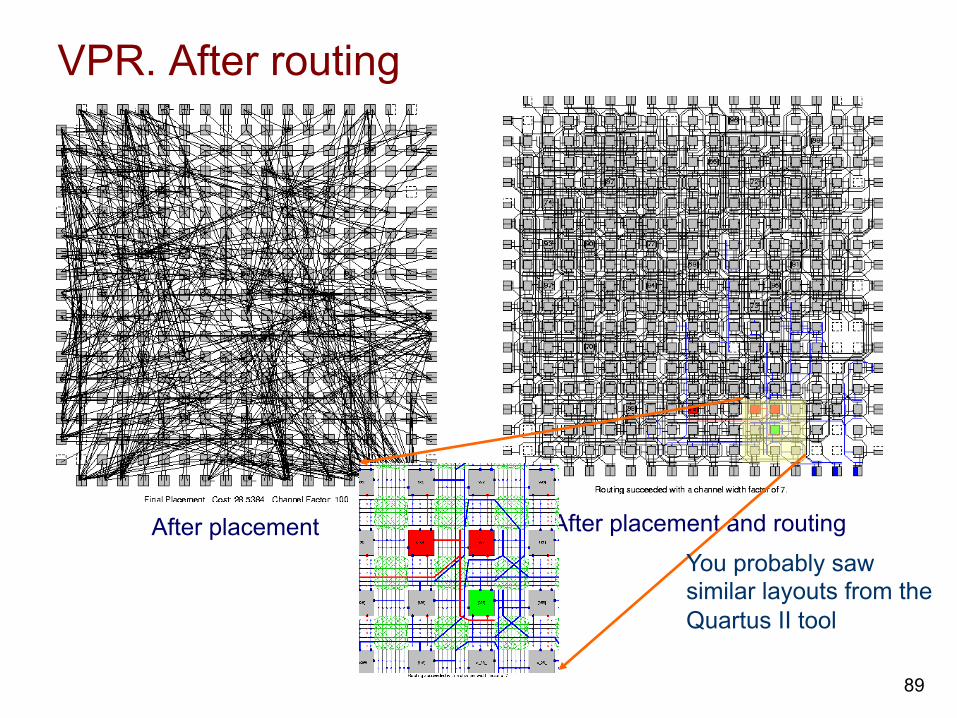
VPR. After routing
After placement After placement and routing
You probably saw similar layouts from the Quartus II tool
89
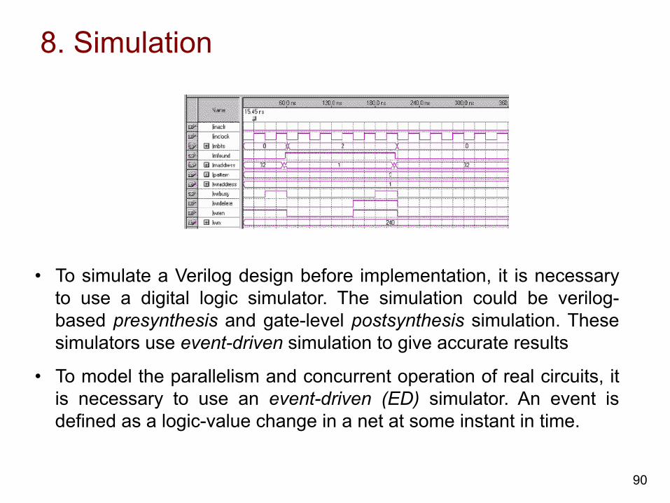
8. Simulation
• To simulate a Verilog design before implementation, it is necessary to use a digital logic simulator. The simulation could be verilog-based presynthesis and gate-level postsynthesis simulation. These simulators use event-driven simulation to give accurate results
• To model the parallelism and concurrent operation of real circuits, it is necessary to use an event-driven (ED) simulator. An event is defined as a logic-value change in a net at some instant in time.
90
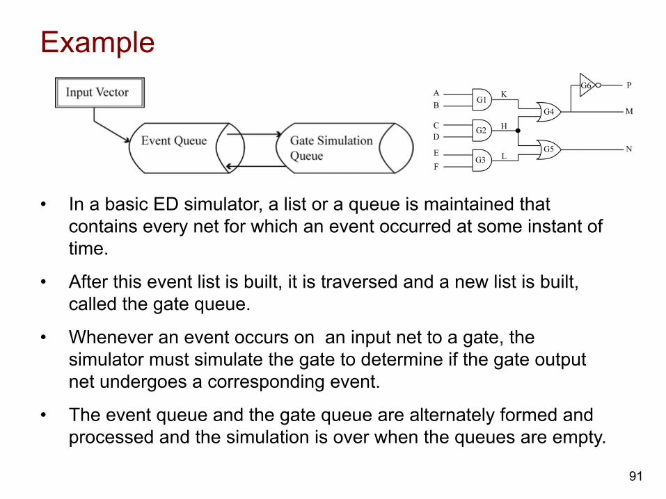
Example
• In a basic ED simulator, a list or a queue is maintained that contains every net for which an event occurred at some instant of time.
• After this event list is built, it is traversed and a new list is built, called the gate queue.
• Whenever an event occurs on an input net to a gate, the simulator must simulate the gate to determine if the gate output net undergoes a corresponding event.
• The event queue and the gate queue are alternately formed and processed and the simulation is over when the queues are empty.
91
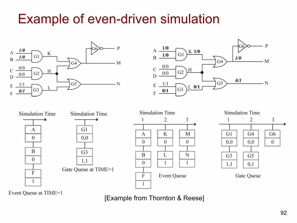
Example of even-driven simulation
[Example from Thornton & Reese]
92
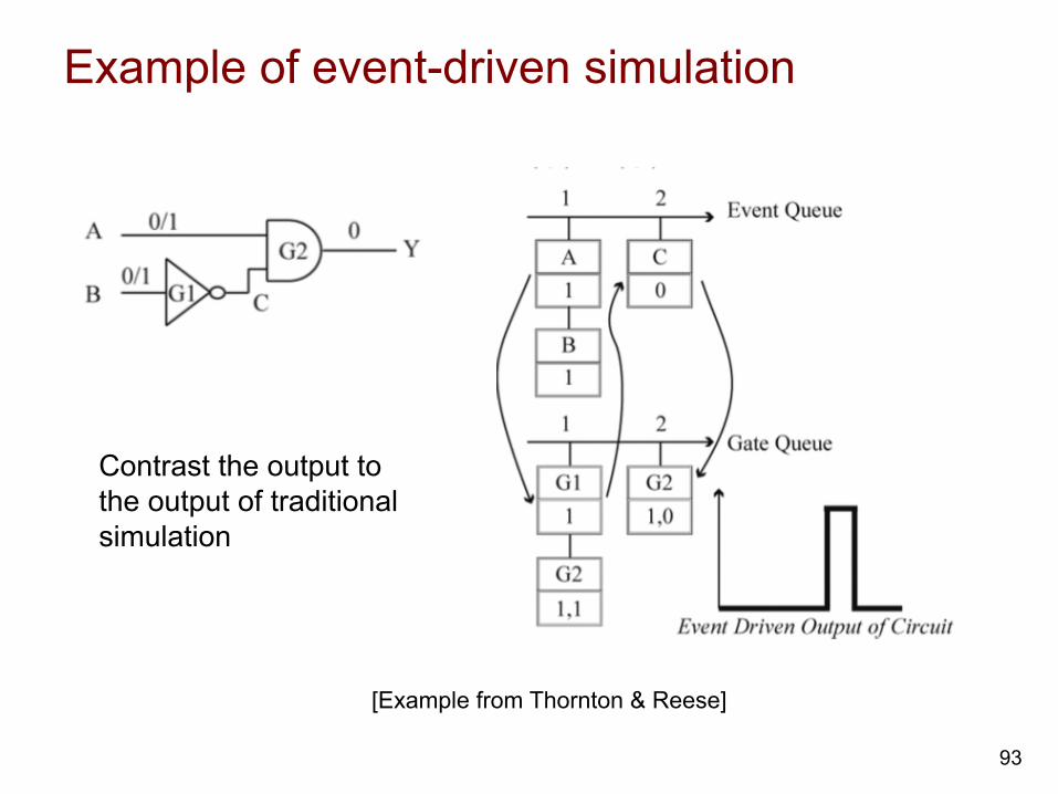
Example of event-driven simulation
Contrast the output to the output of traditional simulation
[Example from Thornton & Reese]
93

Presynthesis vs. postsynthesis simulation
[Example from Thornton & Reese]
94
Ø Synthesis after routing will use most accurate timing info
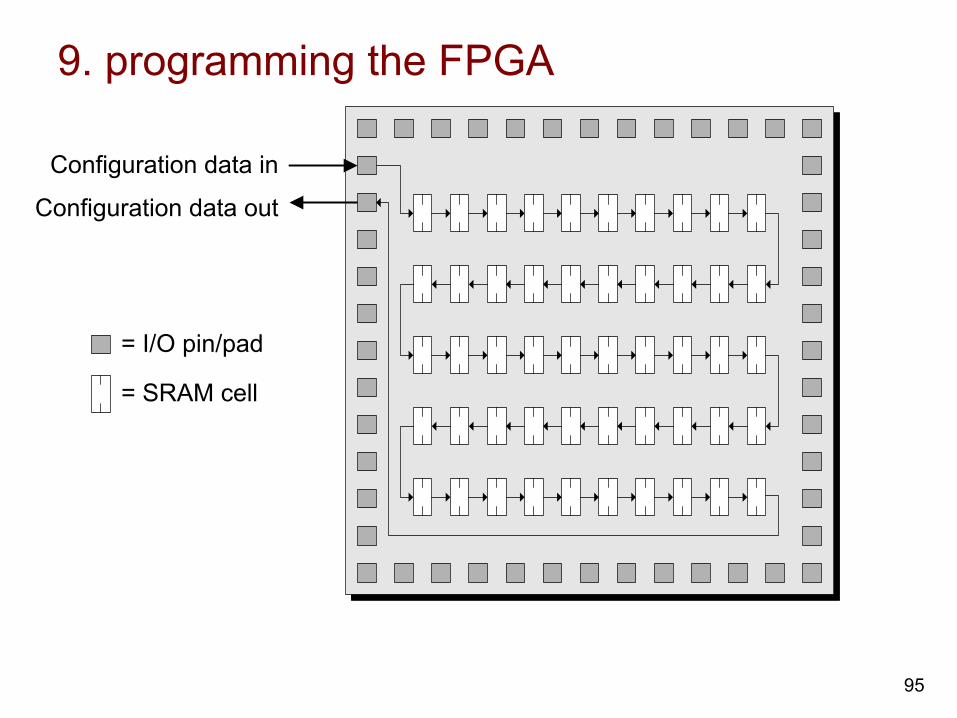
9. programming the FPGA
Configuration data in
Configuration data out
= I/O pin/pad
= SRAM cell
95
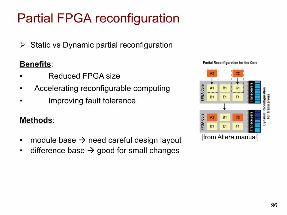
Partial FPGA reconfiguration
96
Ø Static vs Dynamic partial reconfiguration Benefits: • Reduced FPGA size • Accelerating reconfigurable computing • Improving fault tolerance Methods: • module base à need careful design layout • difference base à good for small changes
[from Altera manual]
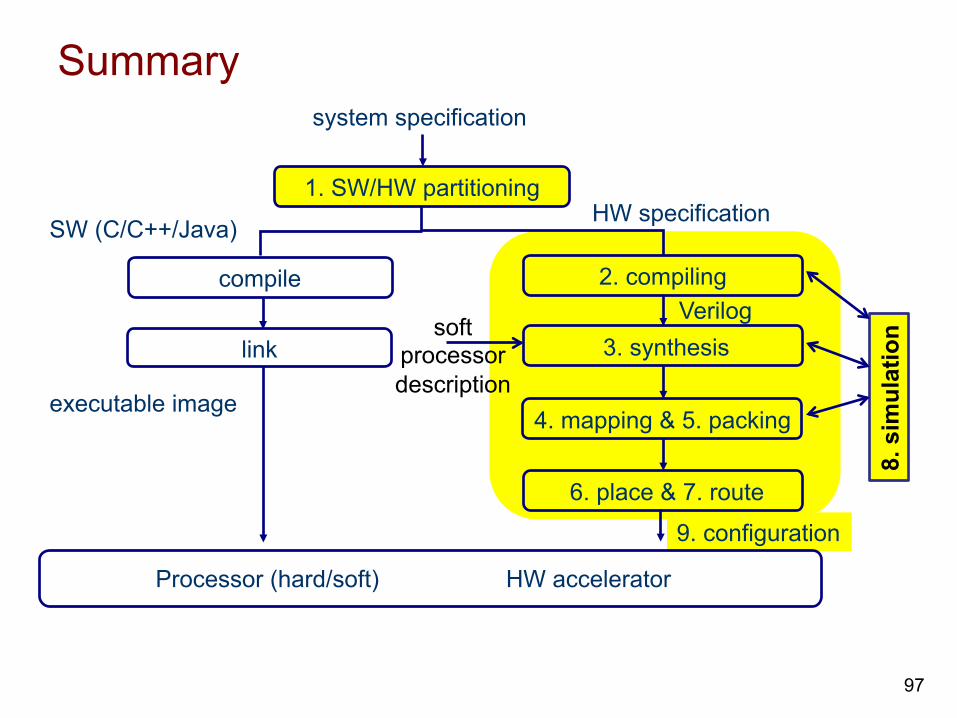
Summary
97
1. SW/HW partitioning
SW (C/C++/Java) HW specification
2. compiling Verilog
3. synthesis
4. mapping & 5. packing
6. place & 7. route
Processor (hard/soft)
compile
link
9. configuration
executable image
HW accelerator
soft processor description
8. s
imul
atio
n
system specification