Empirical Analysis of Limit Order Markets∗

Burton Hollifield†

Robert A. Miller‡

Patrik Sandas§

April, 2002Revised: February, 2003

Abstract

We provide empirical restrictions of a model of optimal order submissions in a limit ordermarket. A trader’s optimal order submission in our model depends on the trader’s valuationfor the asset and the trade offs between order prices, execution probabilities and picking offrisks. The optimal order submission strategy is a monotone function of a trader’s valuation forthe asset. We use the monotonicity restriction to test if the traders follow the optimal ordersubmission strategy in our sample, using the order prices, execution probabilities and pickingoff risks of the orders chosen by the traders in the sample. We compute a semiparametric testusing a sample of order submissions from the Stockholm Stock Exchange. We do not reject themonotonicity restriction for buy orders or sell orders separately, but do reject the monotonicityrestriction when we combine buy and sell orders. The expected payoffs from submitting limitorders away from the quotes are too low relative to the expected payoffs from submitting limitorders close to the quotes to rationalize all the observed order submissions in our sample.

Keywords: limit orders; market orders; order submission strategy; semiparametric estimationJEL Codes: G10, C14, C35, C52

∗We would like to thank Aydogan Alti, Dan Bernhardt, Bruno Biais, David Brown, George Deltas, Zvi Eckstein,Ron Goettler, Pierre Hillion, Ananth Madhavan, Jonas Niemeyer, Christine Parlour, John Rust, Duane Seppi, andparticipants at many different workshops for useful comments. We also thank the Stockholm Stock Exchange, Stock-holms Fondbors Jubileumsfond, and Dextel Findata AB for providing the sample. Hollifield gratefully acknowledgesfinancial support from the Social Sciences Research Council of Canada and the Vancouver Stock Exchange. Part ofthis research was conducted while Hollifield was with the Faculty of Commerce at University of British Columbia.Sandas gratefully acknowledges financial support from the Alfred P. Sloan and the W.L. Mellon Foundations.

†Corresponding author: Graduate School of Industrial Administration, Carnegie Mellon University, Pittsburgh,PA, 15213, e-mail: burtonh@andrew.cmu.edu

‡Graduate School of Industrial Administration, Carnegie Mellon University§The Wharton School, University of Pennsylvania, and CEPR

1 Introduction

Many financial assets trade in limit order markets. In a limit order market, traders can submit

market orders and limit orders. A market order fills immediately at the most attractive price posted

by previously submitted limit orders in the limit order book. A limit order specifies a particular

price, but does not guarantee that the order will be filled. Unfilled limit orders enter the limit order

book, where they are stored until they are canceled or filled by market orders.

A limit order offers the trader a better price than a market order, but there are costs to

submitting a limit order. A limit order may fail to fill; we call the probability that a limit order fills

the execution probability. A limit order may take time to fill. If the trader does not continuously

monitor the limit order, then the limit order may fill when there is a change in the asset value; we

call the expected loss from such fills the picking off risk. Many theoretical models of optimal order

submissions are based on the trade offs between order prices, execution probabilities and picking

off risks. For example, in Cohen, Maier, Schwartz, and Whitcomb (1981); Foucault (1999); Harris

(1998); and Parlour (1998), market and limit order submitters consider the trade offs. In Biais,

Martimort, and Rochet (2000); Glosten (1994); and Seppi (1997) limit order submitters consider

the trade offs.

Empirically, traders change their order submissions as market conditions change. Traders typi-

cally observe information on the number of unfilled limit orders in the book; as well as the bid-ask

spread, equal to the difference between the prices of the lowest priced sell limit order and highest

priced buy limit order in the book. Biais, Hillion, and Spatt (1995) find that traders in the Paris

Bourse are more likely to submit limit orders when the limit order book contains relatively few

orders; or when the bid-ask spread widens. Similar results are found for other limit order markets:

see, for example, Griffiths, Smith, Turnbull, and White (2000) and Ranaldo (2002). If the execu-

tion probabilities for limit orders increase when there are fewer orders in the limit order book or

when the bid-ask spread widens, the evidence may be consistent with the traders responding to

changes in the trade offs. Harris and Hasbrouck (1996) find that the expected payoffs from limit

orders relative to market orders increase when the bid-ask spread widens on the New York Stock

Exchange. Traders change their order submission strategies as the bid-ask spread widens, tending

to submit more limit orders. But are the traders’ order submissions consistent with the theories

1

based on the trade offs?

We show how to determine if the traders’ order submissions are consistent with theories based

on the trade offs. We provide empirical restrictions of a model of optimal order submissions based

on the trade offs, and develop a semiparametric test of them. We compute the test using the order

flow and the limit order book for Ericsson, one of the most actively traded stocks on the Stockholm

Stock Exchange.

A trader’s optimal order submission in our model depends on the trader’s valuation for the asset,

and the trade offs between the order price, the execution probability and the picking off risk of

alternative order submissions. The optimal order submission strategy is a monotone step function

of the trader’s valuation, characterized in terms of threshold valuations. The threshold valuations

are functions of the order prices and the trader’s subjective beliefs about the execution probabilities

and picking off risks. If the traders’ actual order submissions follow the optimal order submission

strategy, then the threshold valuations evaluated at the order prices, execution probabilities and

picking off risks of the traders’ actual order submissions must form a monotone sequence. We use

the actual order submissions, and the realized order fills to form estimates of execution probabilities

and picking off risks. We use the estimates of the execution probabilities and picking off risks to

form estimates of the threshold values at the actual order submissions, and test if they form a

monotone sequence. The test does not require knowledge of the traders’ valuations for the asset,

nor knowledge of the execution probabilities and picking off risks of orders not submitted by the

traders.

A buy limit order fills after it becomes the highest-priced unfilled limit order in the book and

a sell market order is submitted by another trader. Consequently, traders must predict future

traders’ order submissions to determine the execution probabilities and the picking off risks asso-

ciated with alternative order submissions. In a stationary environment, the execution probabilities

and picking off risks associated with alternative order submissions have sample analogues. Hotz

and Miller (1993) and Manski (1993) suggest using nonparametric methods to estimate agents’

conditional expectations to identify and estimate structural models. We follow such an approach,

using nonparametric methods to estimate the execution probabilities and picking off risks for alter-

native order submissions. We condition on information in the limit order book and lagged trading

2

activity to measure information available to the traders.

Our approach is also related to work on the structural estimation of auction models. The

optimal bid in a first-price auction with private values depends on the bidder’s private value and

the trade off between the bid and the probability of the bid winning the auction. Guerre, Perrigne,

and Vuong (2000) show that the observed bid distribution in a first-price private values auction is

consistent with theory if and only if the bid distribution satisfies two conditions. One condition

is that the equilibrium bids must satisfy a monotonicity condition. Guerre, Perrigne, and Vuong

(2000) and Laffont and Vuong (1996) point out that the monotonicity condition can be used to test

the theory. The monotonicity restriction of the optimal order submission strategy that we test is a

necessary condition for optimality of the observed order submissions given the actual dynamics of

the limit order book.

In our sample, we do not reject the monotonicity restriction for buy or sell orders separately

and reject them when we combine buy and sell orders. The expected payoffs from submitting limit

orders with low execution probabilities are too low relative to the expected payoffs from submitting

limit orders with high execution probabilities to rationalize all the order submissions in our sample.

2 Description of the Market and the Sample

In 1990 the Stockholm Stock Exchange completed the introduction of a limit order market system,

the Stockholm Automated Exchange. Here, we briefly describe the Stockholm Automated Exchange

and our sample. There are no floor traders, market makers, or specialists with unique quoting

obligations or trading privileges. Trading is continuous from 10 a.m. to 2:30 p.m. with the opening

price determined by a call auction. All order prices are required to be multiples of a fixed tick size.

When prices are below 100 SKr, the tick size is 1/2 SKr and when prices are above 100 SKr, the

tick size is 1 SKr. During the sample period, $1 was approximately equal to 6.25 SKr. The order

quantity must be a multiple of a round lot, with a typical round lot quantity of 100 shares.

All trading is between market and limit orders. Unfilled limit orders are stored in the electronic

limit order book and are automatically filled by market orders. Unfilled limit orders in the order

book are prioritized first by price and then by time of submission. The prices of the sell limit orders

in the book are called ask quotes and the prices of the buy limit orders in the book are called bid

3

quotes. If a market order is for a smaller quantity than the quantity at the best quote in the limit

order book, the market order will completely fill at a price equal to the best quote. If a market

order cannot be filled completely at the best quote, it will transact with multiple quotes in the

book until either it is completely filled or the book is empty. Any unfilled portion of a market order

converts into a limit order.

A limit order can be canceled at any time at no cost. Traders can also submit hidden limit

orders, where only a portion of the order quantity is displayed in the order book. The hidden part

of a limit order has lower priority than all displayed limit orders at the same order price level.

Orders can only be directly submitted to the trading system by exchange member firms. A

member firm submits orders as a broker for its customers and as a dealer for itself. During our

sample period, there were 24 exchange member firms. We refer to the member firms as brokers.

The brokers are directly connected to the trading system and observe all price quotes with the

corresponding total order quantities in the limit order book. The brokers’ information is updated

almost instantaneously after order submissions or cancellations. Traders who are not directly

connected to the system can obtain information about the five best bid and ask quotes and the

corresponding order quantities in the limit order book through information vendors such as Reuters

or Telerate.

The Stockholm Stock Exchange was the only authorized marketplace for equity trading in

Sweden until January 1, 1993. But many of the stocks listed on the exchange were also cross-

listed on foreign exchanges; trading in London on the international Stock Exchange Automated

Quotation (SEAQ) system and in the United States on the National Association of Securities

Dealers Automated Quotation (NASDAQ) system accounted for a significant fraction of the trading

of many Swedish stocks.

Brokers can settle trades larger than 100 round lots outside the Stockholm Automated Exchange

system. An internal cross is a trade of 100-500 round lots where the broker represents both sides

of the trade. A block trade is a trade greater than 500 round lots.

We obtained the order records and the trade records directly from the Stockholm Automated

Exchange system for the 59 trading days between December 3, 1991, and March 2, 1992 for Ericsson.

The order records is a chronological list of order submissions, changes in the outstanding order

4

quantities, and order cancellations. The trade records is a chronological list of transactions. Each

limit order receives a unique code, and subsequent changes in the outstanding order quantity are

recorded using the same code. We combine changes in the outstanding order quantity and the

transactions to determine whether a change in the order quantity was caused by a trade or a

cancellation. We reconstruct complete transaction and cancellation histories for limit orders and

the entire history of the order book over our sample.

We have detailed information, but there are limitations. We only identify the broker submitting

the order; we cannot separately identify the orders that a broker submits for his customers from

the orders that a broker submits for himself. We also do not observe whether or not an order

includes a hidden order quantity component. We only infer that an order must have involved a

hidden portion if the displayed portion of the hidden order is executed in full. In our sample, there

are few hidden orders whose displayed portions do fully execute. The first limitation causes us to

focus on how a representative trader decides on his order submissions.

Some limit orders remain in the order book at the end of our sample period. To minimize the

effects of the resulting censoring bias on our empirical work, we do not use orders submitted during

the last two days of our sample. Only 2.8% of the orders remain in the system for more than

two trading days, and 62.3% of such orders are eventually canceled. We discard orders submitted

during the first three minutes of the trading day to ensure that the sample reflects only continuous

trading. The filtering rules leave us with 20,760 observations of individual order submissions and

their realized fills.

Table 1 reports descriptive statistics on the daily trading activity for Ericsson. The tick size

varies between 1/2 SKr and 1 SKr since the price fluctuates below and above 100 SKr. The

mean daily close-to-close return is 0.21% with a standard deviation of 3.04%. For comparison, the

table also reports statistics on close-to-close returns computed using prices of Ericsson shares on

NASDAQ from January 2, 1989, through to December 31, 1993, using data from the Center for

Research in Security Prices. The return distribution in our sample is not unusual.

The fourth row of Table 1 reports information on the daily number of active brokers in Ericsson.

All 24 brokers are active in Ericsson over the sample period. Sorting the brokers by their share of

trading volume, the top 3 brokers each transact 10% to 11%, and the next 7 brokers each transact

5

5% to 9%. The shares are almost identical for order submissions. No single broker dominates the

trading of Ericsson.

The fifth row of Table 1 reports the daily trading volume on the Stockholm Automated Ex-

change. The sixth through eight rows of Table 1 report descriptive statistics for orders crossed

internally by brokers, block trades during regular trading hours, and after-hours trading. The

ninth row reports the total trading volume. In our subsequent analysis, we focus on traders’ order

submissions within the Stockholm Automated Exchange and abstract from traders’ decisions to

use the automated system itself or not.

The first column of Table 2 reports the number of buy and sell market and limit orders. The

second column reports the mean execution probabilities, equal to the mean of the fraction of the

limit order quantity that is filled within two trading days of order submission. The execution

probabilities show the unconditional trade off between the execution probability and the order

price; limit orders at prices farther away from the quotes have lower execution probabilities than

limit orders with prices closer to the quotes. The third column of Table 2 reports the mean time-

to-fill for limit orders. Limit orders at prices farther away from the quotes take longer to fill than

limit orders at prices closer to the quotes. The final three columns of Table 2 report the mean and

standard deviation of the order quantity.

The top plot in Figure 1 is the sample survivor function for limit orders. The sample survivor

function evaluated at t is the probability that a limit order remains outstanding for at least t

minutes. When a limit order is partially filled at time t, we weight the fill time by the fraction of

the submitted order quantity filled. Subsequent order fills or cancellations are weighted in the same

manner. Most limit orders leave the book quickly; only 4.6% of the limit orders last for more than

one trading day (270 minutes). The bottom two plots in Figure 1 show the cumulative distribution

function for order fill and cancellation times. Most fills or cancellations occur within three hours

of the order submission.

The first six rows of Table 3 report information about the order quantities in the limit order

books. The average quantity at the best bid or ask quote is roughly nine times the average market

order quantity; only 12 market orders in our sample are for quantities that are larger than the

quantities available in the order book at the best quote at the time of order submission. The order

6

quantities in the limit order book are volatile. The standard deviations of the order quantities at

the three best bid or ask quote levels are all greater than 173 round lots. The standard deviations

of the cumulative order quantities are all greater than 294 round lots.

The last six rows of Table 3 provide information on the bid-ask spread and the distances between

prices quotes in the book. The bid-ask spread is typically is one tick and relatively constant over

our sample. The distances between other price quotes in the book behave similarly.

On average, there is a trade off between order price, execution probability and the length of

time that an order remains unfilled in the limit order book. While most orders are either filled or

canceled quickly, the mean time-to-fill is more than an hour for two and three tick limit orders.

When time elapses between order submission and execution, the order may fill when there is change

in the asset’s value; limit orders may face picking off risk. Finally, the number of orders in limit

order book itself is volatile — observing such information may help a trader predict execution

probabilities and picking off risks. In the next section, we model a representative trader’s optimal

order submission strategy in such a market.

3 Model

At time t, one trader has the opportunity to submit an order. The trader is risk neutral, character-

ized by his valuation for the asset, vt, and the quantity that he wishes to trade, qt. We decompose

vt into two components,

vt = yt + ut. (1)

The random variable yt is the common value of the asset at t; one interpretation is that it is

equal to the traders’ expectations of the liquidation value of the asset. The common value changes

as the traders learn new information, with

yt+1 = yt + δt+1. (2)

Innovations in the common value δt+1 satisfy

Et[δt+1] = 0, (3)

7

where the subscript t denotes conditioning on information available after the common value is

known at t, but before the trader at t arrives. The distribution of common value innovations

has bounded support. Common value innovations are drawn from a stationary process, and the

distribution of the innovations is conditioned on the history of common value innovations through a

finite dimensional set of sufficient statistics. Conditioning on a set of sufficient statistics allows for

persistence in the higher-order moments of the innovations. For example, current common value

volatility may depend on lagged common value volatility.

The random variable ut is the trader’s private value for the asset. Different traders can have

different private values— heterogeneity in the traders’ private values for the asset creates potential

gains from trade. Traders may have different private values as a result of endowment shocks or

differences in their current portfolios. The private value is drawn from a continuous distribution

Prt (ut ≤ u) ≡ Gt(u), (4)

where, as above, the subscript t denotes conditioning on information available after the common

value is known at t, but before the trader at t arrives. The distribution of the private value

has bounded support. The private value is drawn from a stationary process and the conditional

distribution of the private value depends on the same finite dimensional vector of sufficient statistics

as the conditional distribution of common value innovations. For example, the current distribution

of the private values may depend on lagged common value volatility. Once a trader arrives at the

market, his private value remains fixed while he has an order outstanding.

At a random time, t+τcancel, after the trader arrives at the market, the payoff from any unfilled

limit orders submitted by the trader will go to zero, causing the trader to cancel any unfilled limit

orders. The trader does not know the cancellation time at time t. The conditional distribution of

the cancellation time depends on the same finite dimensional vector of sufficient statistics as the

common value innovations. For example, the distribution of the cancellation time may depend on

lagged common value volatility. Let Υ < ∞ be the maximum possible lifetime of the order,

Prt(τcancel ≤ Υ < ∞) = 1. (5)

8

The trader’s desired order quantity, qt, is independent of the trader’s valuation, and is drawn

from a distribution with bounded support. The conditional distribution of the order quantity

depends on the same set of sufficient statistics as the common value innovations. For example, the

distribution of order quantity may depend on lagged common value volatility.

At t, the trader has a single opportunity to submit either a market order or a limit order. The

trader observes the queue of orders in the limit order book, the current common value, and the

history of common value innovations. The trader pays a cost of c per share to submit an order.

The cost is the same for all types of orders submitted.

The decision indicators dsellt,s ∈ {0, 1} for s = 0, 1, . . . , S, and dbuy

t,b ∈ {0, 1} for b = 0, 1, . . . , B

denote the trader’s order submission at t. The trader chooses from a finite set of order prices:

S < ∞ and B < ∞. If the trader submits a sell market order, the order price is the best bid quote

and dsellt,0 = 1. If the trader submits a sell limit order at the price s ticks above the current best bid

quote, dsellt,s = 1. If the trader submits a buy market order, the order price is the best ask quote and

dbuyt,0 = 1. If the trader submits a buy limit order at the price b ticks below the current best ask

quote, dbuyt,b = 1. If the trader does not submit any order at time t, dsell

t,s = 0 for all s and dbuyt,b = 0

for all b.

Suppose a trader with valuation vt = yt + ut at t submits a buy order of quantity qt at a price

pt,b, b ticks below the current best ask quote: dbuyt,b = 1. Define dQt,t+τ as the number of shares

of the order submitted at t that transact at t + τ . If the realized cancellation time is t + τcancel,

dQt,t+τ = 0 for all τ ≥ τcancel. If the trader submits a limit order, he will not know when the order

will execute in the future: dQt,t+τ for τ > 0 is a random variable. For any possible realization of

the future order flow, the future common value and the cancellation time, the total quantity of the

order that eventually transacts must be less than the order quantity:

Υ∑

τ=1

dQt,t+τ ≤ qt. (6)

The payoff that the trader receives from transacting dQt,t+τ at time t + τ at price pt,b is

dQt,t+τ (yt+τ + ut − pt,b) = dQt,t+τ (vt − pt,b) + dQt,t+τ (yt+τ − yt) , (7)

9

where yt+τ is the common value at t+τ . The term dQt,t+τ (vt − pt,b) is the payoff that a transaction

of dQt,t+τ would earn upon immediate execution at price pt,b. The term dQt,t+τ (yt+τ − yt) is the

number of shares transacted in τ periods multiplied by the change in the common value. Summing

over all possible transaction times for the order and including the cost of submitting the order, the

realized payoff is

Ut,t+Υ =Υ∑

τ=0

dQt,t+τ (vt − pt,b) +Υ∑

τ=0

dQt,t+τ (yt+τ − yt)− qtc. (8)

We define the execution probability as

ψbuyt (b, qt) ≡ Et

[Υ∑

τ=0

dQt,t+τ

qt

∣∣∣∣∣ dbuyt,b = 1, qt

](9)

and the picking off risk as

ξbuyt (b, qt) ≡ Et

[Υ∑

τ=0

dQt,t+τ

qt(yt+τ − yt)

∣∣∣∣∣ dbuyt,b = 1, qt

]. (10)

The conditional expectations in equations (9) and (10) do not depend on the trader’s private value.

If the order is a market order, the execution probability is one and the picking off risk is zero. In

taking the expectations in equations (9) and (10), the trader is accounting for the different possible

realizations of other traders’ future order submissions, future common values, and cancellation

times.

The trader’s expected payoff is the expected value of equation (8), conditional on the trader’s

information set, which includes the current limit order book; the current common value; the history

of common value innovations; the trader’s private value; the trader’s order quantity; and the trader’s

order submission:

Et

[Ut,t+Υ

∣∣∣dbuyt,b = 1, ut, qt

]= qtψ

buyt (b, qt) (vt − pt,b) + qtξ

buyt (b, qt)− qtc. (11)

The first term in the trader’s expected payoff is the expected number of shares that will even-

tually transact multiplied by the payoff per share for an immediate transaction at price pt,b. The

second term in the trader’s expected payoff is the covariance of changes in the common value with

10

the quantity of the order that transacts. The final term in the trader’s expected payoff is the cost

of submitting the order. The expected payoff to a trader submitting a sell order for qt shares at a

price s ticks above the current best bid quote is defined similarly.

The trader submits the order that maximizes his expected payoff, conditional on his information,

private value, and order quantity qt,

max{dsell

t,s }S

s=0,n

dbuyt,b

oB

b=0

S∑

s=0

dsellt,s Et

[Ut,t+Υ

∣∣∣dsellt,s = 1, ut, qt

]+

B∑

b=0

dbuyt,b Et

[Ut,t+Υ

∣∣∣dbuyt,b = 1, ut, qt

], (12)

subject to:

dsellt,s ∈ {0, 1}, for s = 0, 1, . . . , S, dbuy

t,b ∈ {0, 1}, for b = 0, 1, . . . , B, (13)

S∑

s=0

dsellt,s +

B∑

b=0

dbuyt,b ≤ 1. (14)

Equation (14) is the constraint that at most one order is submitted. Let dsell∗t (s, ut, qt) and

dbuy∗t (b, ut, qt) be the optimal strategy, detailing the trader’s submission as a function of his be-

liefs and information, private value, and order quantity.

Lemma 1 Suppose that a trader with private value u and quantity q optimally submits a buy order

at price b ≥ 0 ticks below the ask quote: dbuy∗t (b, u, q) = 1.

1. A trader with private value u′ > u and quantity q submits a buy order at a price b′ ticks below

the ask quote: dbuy∗t (b′, u′, q) = 1, with the execution probability higher at b′ than at b,

ψbuyt (b′, q) ≥ ψbuy

t (b, q). (15)

2. Suppose that the execution probabilities are strictly decreasing in the distance between the limit

order price and the best ask quote, ψbuyt (j +1, q) < ψbuy

t (j, q), for all j = 0, 1, . . . , B−1. Then

a trader with private value u′ > u for q shares submits a buy order at a price b′ ticks below

the ask quote: dbuy∗t (b′, u′, q) = 1, with b′ ≤ b.

Similar results hold on the sell side.

The optimal order submission depends on the trader’s valuation. The common value is fixed at

11

t so that the only source of heterogeneity in the decision at t is the trader’s private value. If the

trader buys, the higher the trader’s private value, the higher the execution probability is for the

trader’s optimal buy order. If the trader sells, the lower the trader’s private value, the higher the

execution probability is for the trader’s optimal sell order.

Lemma 1 and the discrete price grid imply that we can partition the set of valuations into

intervals. All traders wishing to trade the same quantity whose valuations lie within the same

interval submit the same order. Define the threshold valuation θbuyt (b, b′, q) as the valuation of a

trader who is indifferent between submitting a buy order at price pt,b and a buy order at price pt,b′ ,

θbuyt

(b, b′, q

)= pt,b +

(pt,b − pt,b′

)ψbuy

t (b′, q) +(ξbuyt (b′, q)− ξbuy

t (b, q))

ψbuyt (b, q)− ψbuy

t (b′, q). (16)

The threshold valuation for a buy order at price pt,b and not submitting an order is

θbuyt (b,NO, q) = pt,b +

−ξbuyt (b, q) + c

ψbuyt (b, q)

. (17)

The threshold valuation for a sell order at price pt,s and a sell order price pt,s′ is

θsellt

(s, s′, q

)= pt,s −

(pt,s′ − pt,s

)ψsell

t (s′, q) +(ξsellt (s, q)− ξsell

t (s′, q))

ψsellt (s, q)− ψsell

t (s′, q). (18)

The threshold valuation for a limit sell order at price pt,s and not submitting any order is

θsellt (s,NO, q) = pt,s − ξsell

t (s, q) + c

ψsellt (s, q)

. (19)

The threshold valuation for a sell order at price pt,s and a buy order at price pt,b is

θt (s, b, q) = pt,s +(pt,b − pt,s) ψbuy

t (b, q)−(ξsellt (s, q) + ξbuy

t (b, q))

ψsellt (s, q) + ψbuy

t (b, q). (20)

Let B∗t (q) index the set of buy order prices that are optimal for some trader who wishes to trade

q shares at time t,

B∗t (q) ≡{

b∣∣∣dbuy∗

t (b, u, q) = 1 for some u}

, (21)

12

with elements b∗i,t(q), for i = 1, . . . , I, ordered by the execution probabilities,

ψbuyt (b∗i,t(q), q) > ψbuy

t (b∗i+1,t(q), q). (22)

Let S∗t (q) index the set of sell order prices that are optimal for some trader who wishes to trade q

shares at time t, with elements s∗j,t(q), for j = 1, . . . , J , ordered by the execution probabilities.

Lemma 2

θbuyt

(b∗1,t(q), b

∗2,t(q), q

)> θbuy

t

(b∗2,t(q), b

∗3,t(q), q

)> . . . > θbuy

t

(b∗I−1,t(q), b

∗I,t(q), q

), (23)

θsellt

(s∗J−1,t(q), s

∗J,t(q), q

)> θsell

t

(s∗J−2,t(q), s

∗J−1,t(q), q

)> . . . > θsell

t

(s∗1,t(q), s

∗2,t(q), q

), (24)

θbuyt

(b∗I−1,t(q), b

∗I,t(q), q

)> θt

(s∗J,t(q), b

∗I,t(q), q

)> θsell

t

(s∗J−1,t(q), s

∗J,t(q), q

). (25)

To describe the optimal decision rule, define the marginal thresholds for sellers and buyers as

θbuyt (Marginalt(q), q) = max

(θt

(s∗J,t(q), b

∗I,t(q), q

), θbuy

t

(b∗I,t(q), NO, q

)),

θsellt (Marginalt(q), q) = min

(θt

(s∗J,t(q), b

∗I,t(q), q

), θsell

t

(s∗J,t(q),NO, q

)). (26)

If the buyer and seller marginal thresholds are equal to each other, all traders find it optimal to

submit an order. Otherwise, some traders find it optimal not to submit any order.

Lemma 3 The optimal order submission strategy is

dbuy∗t (b, u, q) = 1, if

b = b∗1,t(q) and

θbuyt (b∗1,t(q), b

∗2,t(q), q) ≤ yt + u < ∞,

or

b = b∗i,t(q) for i = 2, ..., I − 1 and

θbuyt (b∗i,t(q), b

∗i+1,t(q), q) ≤ yt + u < θbuy

t (b∗i−1,t(q), b∗i,t(q), q),

or

b = b∗I,t(q) and

θbuyt (Marginalt(q), q) ≤ yt + u < θbuy

t (b∗I,t(q), b∗I−1,t(q), q),

(27)

13

dsell∗t (s, u, q) = 1, if

s = s∗1,t(q), and

−∞ ≤ yt + u < θsellt (s∗1,t(q), s

∗2,t(q), q),

or

s = s∗j,t(q), for some j = 2, . . . , J − 1 and

θsellt (s∗j−1,t(q), s

∗j,t(q), q) ≤ yt + u < θsell

t (s∗j,t(q), s∗j+1,t(q), q),

or

s = s∗J,t(q), and

θsellt (s∗J−1,t(q), s

∗J,t(q), q) ≤ yt + u < θsell

t (Marginalt(q), q),

(28)

otherwise,

dbuy∗t (b, u, q) = dsell∗

t (s, u, q) = 0. (29)

Let Vt(yt+u, q) be the indirect utility function for a trader at t with valuation yt+u and quantity

q. The indirect utility function is computed by substituting the optimal strategy in equations (27)

through (29) into the trader’s objective function, equation (12).

Lemma 4 Vt(yt + u, q) has the following properties.

1. Vt(yt + u, q) is a positive, convex function of yt + u.

2. Suppose that dbuy∗t (b, u, q) = 1 for some (b, u, q). Then for u′ > u, Vt(yt +u′, q) > Vt(yt +u, q).

3. Suppose that dsell∗t (s, u, q) = 1 for some (s, u, q). Then for u′ < u, Vt(yt+u′, q) > Vt(yt+u, q).

Figure 2 provides an example of Vt(yt + u, q). Here, S∗t (1) = {0, 1, 2} and B∗t (1) = {0, 1, 2}:market, one tick, and two tick limit buy and sell orders are optimal for a trader with some valuation

and the order quantity is one share. The expected payoffs as a function of the trader’s valuation

from submitting sell orders are plotted with dashed lines and the expected payoffs from submitting

buy orders are plotted with dashed-dotted lines. From equation (11), the trader’s expected payoff

from submitting any particular order is a linear function of his valuation, with slope equal to the

execution probability for that order. The indirect utility function is plotted with a thick solid line

and is the upper envelope of the payoffs for different order submissions.

A change in the cost of submitting the order, c, leads to a parallel shift in the expected payoff

from all order submissions. A change in the picking off risk for any particular order leads to a parallel

14

shift in the expected payoff from submitting that particular order, while keeping unchanged the

expected payoff from submitting any other order. A change in the execution probability for any

particular order leads to a shift in the slope in the expected payoff from submitting that particular

order, while keeping unchanged the expected payoff from submitting any other order.

Geometrically, the thresholds are the valuations for which the expected payoffs intersect. For

example, the threshold for a sell market order and a sell limit order at one tick from the best

bid quote is θsellt (0, 1, 1); a trader with a valuation less than θsell

t (0, 1, 1) submits a sell market

order. The thresholds associated with submitting any particular order and submitting no order

are the valuations where the expected payoffs cross the horizontal axis. Here, θsellt (2, NO, 1) <

θt (2, 2, 1) , and θbuyt (2,NO, 1) > θt (2, 2, 1) . If the trader’s valuation is between θsell

t (2, NO, 1) and

θbuyt (2,NO, 1), the trader does not submit any order.

Consider increasing the order submission cost, c. The expected payoffs for submitting any order

decrease, with all payoff curves shifting down by the same amount. As a consequence, only the

thresholds associated with submitting an order and submitting no order change. The marginal buy

threshold increases and the marginal sell threshold decreases; more traders will choose not to make

an order submission.

Consider increasing the picking off risk for the one tick sell limit order. The expected payoffs for

submitting a one tick sell order decreases, and the expected payoffs for any other order submissions

do not change. The expected payoffs for a one tick sell limit order make a parallel outward shift,

implying that the threshold for the one tick sell order and the two tick sell order decreases and

the threshold for the one tick sell order and market order increases. The payoff curve for a market

order is steeper than the payoff curve for the two tick sell order; the threshold associated with the

market order increases by less than the threshold associated with the two tick order decreases as a

consequence of increasing the picking off risk.

Consider increasing the execution probability for the one tick sell order. The expected payoffs for

submitting a one tick sell order increase, and the expected payoffs for any other order submissions

do not change, implying that the threshold for the one tick sell limit order and the two tick sell

limit order increases and the threshold for the one tick sell limit order and market order decreases.

The optimal submission strategy in equations (27)–(29) can be used to compute the probability

15

of a trader submitting a sell order at a price s∗1,t(q) ticks above the current best bid quote, conditional

on the arrival of a trader who wishes to trade q shares. Typically, s∗1,t(q) = 0 — a sell market order

is optimal for some trader. The probability is

Prt

(dsell∗ (

s∗1,t(q), ut, q)

= 1∣∣∣ q

)= Prt

(yt + ut ≤ θsell

t

(s∗1,t(q), s

∗2,t(q), q

)∣∣ q)

= Gt

(θsellt

(s∗1,t(q), s

∗2,t(q), q

)− yt

). (30)

The last line follows from the definition of Gt in equation (4) and because the quantity and the

private value are independent random variables. Similarly, for j = 2, . . . , J − 1

Prt

(dsell∗

t

(s∗j,t(q), ut, q

)= 1

∣∣∣ q)

= Gt

(θsellt

(s∗j,t(q), s

∗j+1,t(q), q

)− yt

)−Gt

(θsellt

(s∗j−1,t(q), s

∗j,t(q), q

)− yt

), (31)

and for j = J

Prt

(dsell∗

t

(s∗J,t(q), ut, q

)= 1

∣∣∣ q)

= Gt

(θsellt (Marginalt(q), q)− yt

)−Gt

(θsellt

(s∗J−1,t(q), s

∗J,t(q), q

)− yt

). (32)

Similar expressions to equations (30) through (32) hold for buy orders.

Equations (30) through (32) can be used to interpret previous empirical studies of order sub-

missions. For example, Biais, Hillion, and Spatt (1995) find that a larger ask depth increases the

probability of a sell market order and decreases the probability of a sell limit order. A larger

ask depth may imply a smaller execution probability for a one tick sell limit order, increasing the

threshold valuation for a sell market order and a one tick sell limit order. From equations (30) and

(31), increasing the threshold valuation increases the probability of observing a sell market order

and decreases the probability of a sell limit order.

Biais, Hillion, and Spatt (1995) also find that traders are more likely to submit limit orders

when the bid-ask spread widens. Suppose the bid-ask spread widens from one to two ticks, holding

the best ask quote, the common value, the execution probabilities, and picking off risks constant.

Such an increase in the spread would decrease the threshold for a sell market order and a one tick

16

sell order. From equations (30) and (31), the probability of a sell market order decreases and the

probability of a sell limit order increases. A widening of the spread may also increase the execution

probability for one tick away limit orders. An increase in the execution probability would decrease

the threshold for a sell market order and a one tick sell order. Again, the probability of a sell

market order decreases and the probability of a sell limit increases.

Equations (30) through (32) also provide two ways to interpret the autocorrelation in order

submissions documented in existing empirical work. First, the threshold valuations may be auto-

correlated if the limit order book changes only gradually causing the expected payoffs from different

order submissions to be autocorrelated. Second, innovations in the common value are correlated

with the current order submission, and unless the book adjusts immediately to innovations in the

common value, such common value innovations will cause autocorrelated order submissions.

Figure 3 plots the optimal order submission strategy corresponding to the indirect utility func-

tion in Figure 2. The distribution of private values Gt is a mixture of three normal distributions.

The horizontal axis in the figure is the trader’s private value and the vertical axis is the cumulative

probability distribution of the private values. The probability of various order submissions is deter-

mined by the thresholds, the common value, and the distribution of private values Gt by equations

(30) through (32).

For example, the probability of a trader submitting a sell market order is Gt

(θsellt (0, 1, 1)− yt

).

A trader with valuation between θsellt (1, 2, 1)− yt and θsell

t (0, 1, 1)− yt submits a one tick sell limit

order. The probability of a trader submitting a one tick sell limit order is Gt

(θsellt (1, 2, 1)− yt

)−Gt

(θsellt (0, 1, 1)− yt

). A trader with a private value between θsell

t (2, NO, 1) and θbuyt (2, NO, 1) does

not submit any order, and the probability of such an event is

Prt (NO|q) = Gt

(θbuyt (2, NO, 1)− yt

)−Gt

(θsellt (2,NO, 1)− yt

). (33)

Given that a trader may find it optimal to submit no order, the probability of observing a sell

market order, conditional on observing any order submission, is

Prt

(dsell∗

t

(s∗1,t(q), ut, q

)= 1

∣∣∣ q, order submission)

=Gt

(θsellt (0, 1, 1)− yt

)

1− Prt (NO |q) . (34)

17

From Equations (30) through (32) the conditional probabilities of observing different order

submissions form an ordered qualitative response model, as defined by Amemiya (1985, Definition

9.3.1, page 292). It is possible to use the model to estimate the private value distribution. Of

course the estimates must allow for the possibility that some traders may choose not to make any

order submission.

We use Lemma 2 as a basis of an empirical test of the model. The test does not require

knowledge of Gt but does require knowledge of actual order submissions; their prices, execution

probabilities and picking off risks. The logic of the test is illustrated by the following example.

The conditional probability of observing each of the following buy orders is strictly positive: a buy

market order, a one tick buy limit order, and a two tick buy limit order. The best ask quote is

100, and the tick size is 1. The execution probabilities are ψbuyt (0, 1) = 1, ψbuy

t (1, 1) = 0.7 and

ψbuyt (2, 1) = 0.6. For simplicity, the picking off risk for all buy limit orders is zero. The order

quantity is one share. Observing such data implies that the model is false.

Figure 4 plots the payoffs for a trader submitting the three different buy orders against the

trader’s valuation; a dashed line for a buy market order, a light solid line for a one tick buy limit

order, and a dashed-dotted line for a two tick buy limit order. There is no valuation for which the

one tick buy limit order is optimal; the expected payoff from submitting a one tick buy limit order

is always lower than the payoffs from submitting a market order or a two tick limit order. The

threshold valuations are

θbuyt (0, 1, 1) = 100 +

(1)(0.7)(1.0− 0.7)

= 102.33,

θbuyt (1, 2, 1) = 99 +

(1)(0.6)(0.7− 0.6)

= 105.00. (35)

In the example, θbuyt (1, 2, 1) > θbuy

t (0, 1, 1); the threshold valuations violate the monotonicity

restriction. Since traders submit one tick limit orders with positive probability, the observed order

submissions are not the outcome of the optimization in equations (12) through (14). Computing

the threshold valuations requires only the execution probabilities for the orders that are actually

submitted. It does not require knowledge of the traders’ valuations nor of the distribution of the

traders’ valuations, nor knowledge of the execution probabilities and picking off risks of orders not

18

submitted by the traders.

The example is not a knife-edge case. Hold the execution probability for a market order equal

to one and the execution probability for a two tick limit order equal to 0.6. With execution

probabilities for a one tick limit order between 0.6 and 0.75, the model is inconsistent with traders

submitting a one tick limit order with strictly positive probability. With execution probabilities

for a one tick limit order between 0.75 and 1.00, the model is consistent with traders submitting a

one tick limit order with strictly positive probability.

4 Empirical Evidence

Lemma 2 states that if the traders’ order submissions are the solution to equations (12) – (14),

then the thresholds evaluated at the orders chosen by the traders must form a monotone sequence

when the orders are ranked according to the execution probabilities. We identify orders chosen

by the traders with positive probability in our sample and rank them according to their execution

probabilities. We compute the thresholds at the orders and test the monotonicity property.

We assume that the traders’ conditioning information is measured by a vector of conditioning

variables. Since the model imposes weak functional form restrictions on the execution probabilities

and picking off risks, we estimate the traders’ expectations using nonparametric regressions of

the realized fill history of each of the orders onto a set of conditioning variables. Ideally, we

would include in the conditioning information the order quantity; the entire limit order book; and

information that predicts the distribution of the common value innovations, the distribution of

private values, and the cancellation time. It is impractical to do so. Instead, we condition on six

variables: order quantity, ask depth, bid depth, lagged volume, index volatility, and time of day.

Table 4 contains definitions of the conditioning variables. We choose the conditioning variables on

the basis of the theoretical arguments in Foucault (1999) and Parlour (1998), and the empirical

evidence in Biais, Hillion and Spatt (1995) and Harris and Hasbrouck (1996). Let Xt denote

the conditioning information. In unreported ordered probit models, we reject the null that the

conditioning variables do not predict the traders’ order submissions.1

We include the order quantity since the trade offs between order prices, execution probabilities

and picking off risks are likely to depend on order quantity. Harris and Hasbrouck (1996) show1For buy orders: χ2

6 = 2428.2, with p-value= 0.00 and for sell orders: χ26 = 1622.7, with p-value = 0.00.

19

that in the New York Stock Exchange, an increase order quantity tends to decrease execution

probabilities.

We include the ask and bid depth to capture competition between traders on the same side of the

limit order book. The book quantities reported in Table 3 indicate that the depth is volatile in our

sample. We do not condition on the bid-ask spread, since it is relatively constant over the sample.

The time priority rule implies that a new sell limit order at the best ask quote is likely to have a lower

execution probability when the ask depth is large. The depth on the other side of the book may

also influence the order submissions. A larger bid depth implies more competition among buyers,

increasing the probability of buy market order submissions in the future and therefore increasing

the execution probabilities for new sell limit orders. Such effects occur in the equilibrium in Parlour

(1998).

Biais, Hillion and Spatt (1995) find empirically that trading activity is clustered in time. As

a consequence, lagged trading volume may have an impact on the execution probabilities. In

Foucault’s (1999) theoretical model, the volatility of the asset influences both the execution prob-

abilities and the picking off risks. Such effects are likely to carry over to many formulations of

the order submission problem. We condition on lagged index volatility to measure volatility for

two reasons. First, index volatility measures market-wide volatility and may be less sensitive to

volatility induced by transactions randomly occurring at the best bid or ask quotes than volatility

measured by Ericsson’s transaction price volatility. Second, conditional volatility is autocorrelated.

In Parlour (1998) order submission strategies depend explicitly on the time of day, and Bias,

Hillion, and Spatt (1995) find such effects empirically. Foucault (1999) studies the stationary

equilibrium to an overlapping generations model where orders last one period. The model in

Foucault (1999) could be extended to allow for a time of day effect. For example, if the market

closed every k periods, then we expect that identical traders facing the same book to face different

execution probabilities and picking off risks depending on the time until the next market closing.

4.1 Test of Strictly Positive Conditional Choice Probabilities

Let

B(Xt) ={

b∣∣∣Pr

(dbuy

t,b = 1∣∣∣Xt

)> 0

}(36)

20

index buy order prices that are chosen with strictly positive probability in our sample conditional

on Xt, with a similar definition for S(Xt). Order B(Xt) by the distance from the best ask quote

and order S(Xt) by the distance from the best bid quote.

An order is in B(Xt) or S(Xt) for all Xt, if it has strictly positive conditional choice probability

for all Xt. Suppose that buy orders at n, n + 1, . . . , N and sell orders at o, o + 1, . . . , O all have

conditional choice probabilities greater than or equal to LB, where LB > 0. Let z++t be a vector

of strictly positive measurable functions of the vector Xt, and ⊗ the Kronecker product. Define

PC = E

dbuyt,n − LB

...

dbuyt,N − LB

dsellt,o − LB

...

dsellt,O − LB

⊗ z++t

. (37)

The law of iterated expectations and the restriction that the conditional choice probabilities are

greater than or equal to LB imply the null hypothesis

H0 : PC > 0. (38)

We use the sample moment analogue PCT to form an estimator for PC. Under standard con-

ditions,√

T(PCT − PC

)converges in distribution to a normal random variable, with asymptotic

variance-covariance matrix, APC . Wolak (1989) derives a test statistic for a local test of H0,

MPC = min{a|a≥0}

T (PCT − a)A−1PC(PCT − a)′, (39)

and shows that under H0, MPC converges in distribution to the weighted sum of χ2 variables,

Pr(MPC ≥ r) =dim(APC)∑

k=0

Pr[χ2k ≥ r]w(dim(APC), dim(APC)− k,APC), (40)

where χ2k is a χ2 variable with k degrees of freedom, dim(APC) is the rank of the asymptotic

21

variance-covariance matrix, and w(dim(APC), dim(APC) − k,APC), k = 0, . . . , dim(APC) are a

set of weights that depend on the asymptotic variance-covariance matrix. Wolak (1989) describes

a Monte Carlo method for calculating the weights.

Table 5 reports the results for the tests that the conditional choice probabilities are greater

than 0.02. The tests are computed for one tick, two tick, and three tick buy and sell limit orders.

Table 2 reports that in our sample, approximately 48% of the orders submitted are market orders,

and so we do not include market orders in the test.

Each row reports the point estimates of the unconditional differences in decision indicators and

0.02 multiplied by positive instruments, the associated standard errors, and p-values for the null of

monotonicity of the conditional choice probabilities for different order submissions.2 Each column

corresponds to a different positive instrument. The final row of the table reports the MPC test

described above for each instrument and all submissions, and the final column of the table reports

the test statistic across the instruments. All of the point estimates are strictly positive and none

of the tests reject the null hypothesis of strictly positive choice probabilities; the p-values are all

greater than 0.98.

We find no evidence against the hypothesis that the traders submit one tick, two tick, and

three tick limit orders at each value of the conditioning variables. We compute the thresholds for

market orders and limit orders up to three ticks away from the quotes. A censoring bias could

arise in our subsequent tests if some order submission between a market and three tick limit order

were optimal for some trader, but not used in computing the thresholds. Since we use all order

submissions between a market order and a three tick away limit order, the tests do not face such

a censoring bias.

4.2 Test of Monotonicity of the Execution Probabilities

If execution probabilities are monotone in the distance from the best quotes, then ranking the

order prices by the distance from the best quotes is equivalent to ranking them by their execution

probabilities. The assumption is a weak one in a deep market — a deep market imposes enough

competitive pressure on traders such that they cannot increase execution probabilities by placing2The standard errors are computed with 50 lags using the Newey and West (1987) procedure. The empirical

results are robust to changes in the lag length. The asymptotic p-values for the monotonicity tests are computedusing 10,000 Monte Carlo simulation trials.

22

less aggressive orders.

The execution probabilities are computed as a nonparametric regression of realized fills on

information known at the time of order submission. Let K be a multidimensional kernel function

and hT a bandwidth associated with each argument. The nonparametric estimate of ψsell(s, Xt) is

ψsell(s, Xt) ≡∑T

t′ 6=t

(dsell

t′,s∑Υ

τ=1

dQt′,t′+τ

qt′

)K (

h−1T (Xt′ −Xt)

)∑T

t′ 6=tK(h−1

T (Xt′ −Xt)) , (41)

for s ∈ S(Xt), with a similar definition on the buy side. From the definition of S(Xt), ψsell(s, Xt)

is well defined. Since the lifetime of most limit orders is less than two days in our sample, we set

the maximum lifetime of the order, Υ in equation (41), equal to two days.

Elements of B(Xt) are ordered by the distance from the best ask quote and elements of S(Xt)

by the distance from the best bid quote. To test monotonicity of the execution probabilities, define

DF ≡ E

I(Xt ∈ X)

ψbuy(b1, Xt)− ψbuy(b2, Xt)

ψbuy(b2, Xt)− ψbuy(b3, Xt)...

ψsell(s1, Xt)− ψbuy(s2, Xt)

ψsell(s2, Xt)− ψsell(s3, Xt)...

⊗ z++t

, (42)

where I(Xt ∈ X) is a trimming indicator for the set X in the interior of the support of Xt. The

trimming indicator is used to simplify the asymptotic distribution. Applying the law of iterated

expectations, monotonicity of the execution probabilities implies the null hypothesis

H1 : DF > 0. (43)

We use the sample moment analogue of DF to form the estimator DF T , using the nonparametric

estimators of the execution probabilities. In Appendix C, we provide regularity conditions under

which√

T(DF T −DF

)converges in distribution to a normal random variable, and we provide the

asymptotic variance-covariance matrix, ADF . We form a similar test statistic to MPC in equation

23

(39) above as a test of H1.

Table 6 reports the results of the monotonicity tests of the execution probabilities. The tests

are computed using the execution probabilities for market and one tick limit orders; one and two

tick limit orders; and two and three tick limit orders, for both the buy and sell orders.

Each row reports the point estimates of the unconditional differences in execution probabilities

multiplied by positive instruments, standard errors, and p-values for the null of monotonicity of

the execution probabilities for different order submissions.3 Each column corresponds to a different

positive instrument. The final row of the table reports the MDF test described above for each

instrument and all submissions, and the final column of the table reports the test statistic across

each order submission. All of the point estimates are strictly positive and none of the tests reject

the null hypothesis of monotonicity of the execution probabilities; the p-values are all greater than

0.98.

Together, the test statistics reported in Table 5 and Table 6 fail to reject that market orders,

one tick, two tick, and three tick limit buy and sell orders are chosen for each value of the condi-

tioning information, and that ordering the orders by the distance from the quotes is the same as

ordering them by their execution probabilities. We use the associated threshold valuations to form

a monotonicity test.

4.3 Computing the Threshold Valuations

To compute the threshold valuations, we need estimates of the picking off risks. To form estimates

of the picking off risks, we need estimates of changes in the common value. A common proxy for

the common value in many microstructure applications is the mid-quote, equal to the average of

the best bid and ask quote. Such a proxy is inappropriate in our application for two reasons. First,

a trader influences the current mid-quote by his order submission at time t. Second, a limit order

is executed once it becomes the best bid or ask quote, inducing a mechanical correlation between

the mid-quote and the execution. Our common value is not based on the mid-quote but instead is

based on the level of the market index.3The standard errors are computed with 50 lags using the method described in Appendix C to capture the overlap

in the errors in the execution probabilities between orders submitted at different times. The empirical results arerobust to changes in the lag length. The asymptotic p-values for the monotonicity tests are computed using 10,000Monte Carlo simulation trials.

24

From equation (3), the common value is integrated of order one, or I(1). We assume that there

is an I(1) vector of factors, ft, such that

yt = βft, (44)

with β a parameter.

The best bid quote is observed when there are buy limit orders outstanding in the order book.

Accordingly, denote by t′ a time period where there are outstanding buy limit orders in the book.

We provide conditions in Appendix B for the best bid quote to be co-integrated with the common

value,

psellt′,0 = yt′ + εt′

= βft′ + εt′ , (45)

where psellt′,0 is the best bid quote at time t′ and εt′ is I(0). Let βT ′ denote the least squares estimate

of β obtained by regressing psellt′,0 on ft′ . We form an estimate of the common value as

yt = βT ′ft. (46)

We used minute-by-minute observations of the value of the OMX index as our factor series.

The OMX index is a value-weighted index of the 30 most traded companies on the Stockholm

Stock Exchange. We also experimented with including the daily sampled US/SKr exchange rate

and daily sampled Swedish interest rates as factors. The exchange rate and interest rates added

little explanatory power and we therefore only report the results obtained using the market index.

The first column of Table 7 reports a Dickey-Fuller test statistics for the null hypothesis of a

unit root in the OMX index, the bid quote, and the ask quote; the test fails to reject the null. The

final two columns of Table 7 report our estimate of βT ′ and an Engle-Granger cointegration test.

We reject the null hypotheses that the bid and the ask are not cointegrated with the OMX index.

25

Our estimator for ξsell(s, Xt) is

ξsell(s, Xt) =

∑Tt′ 6=t

(dsell

t′,s∑Υ

τ=0

dQt′,t′+τ

qt′(yt′+τ − yt′)

)K (

h−1T (Xt′ −Xt)

)∑T

t′ 6=tK(h−1

T (Xt′ −Xt)) , (47)

where yt is the estimator of the common value in (46), and s ∈ S(Xt). We form a similar estimator

for buy order picking off risks.

We estimate the threshold valuations by

θsell(s, s′, Xt) = ps,t −(ps′,t − ps,t

)ψsell(s′, Xt) +

(ξsell(s, Xt)− ξsell(s′, Xt)

)

ψsell(s, Xt)− ψsell(s′, Xt), (48)

with a similar estimator for the buy side. If ψsell(s, Xt) − ψsell(s′, Xt) > 0, then θsell(s, s′, Xt)

is a continuous function of the execution probabilities and picking off risks. Consistency of the

estimators for the execution probabilities and picking off risks therefore implies consistency of the

estimator θsell(s, s′, Xt) for the thresholds.

4.4 Test of Monotonicity of the Threshold Valuations

We use our estimators for the threshold valuations, equation (48), to form a test statistic for the

monotonicity restrictions in equation (23) of Lemma 2. If

{0, 1, 2, 3} ⊂ S∗(Xt), and {0, 1, 2, 3} ⊂ B∗(Xt), (49)

Lemma 2 implies

θbuy (0, 1, Xt) > θbuy (1, 2, Xt) > θbuy (2, 3, Xt) , (50)

θsell (2, 3, Xt) > θsell (1, 2, Xt) > θsell (0, 1, Xt) , (51)

and

θbuy (2, 3, Xt) > θsell (2, 3, Xt) . (52)

26

Define

Dθ ≡ E

I(Xt ∈ X)

θbuy (0, 1, Xt)− θbuy (1, 2, Xt)

θbuy (1, 2, Xt)− θbuy (2, 3, Xt)

θsell (1, 2, Xt)− θsell (0, 1, Xt)

θsell (2, 3, Xt)− θsell (1, 2, Xt)

θbuy (2, 3, Xt)− θsell (2, 3, Xt)

⊗ z++t

.

Inequalities (50) through (52) and the law of iterated expectations imply the null hypothesis,

H2 : Dθ > 0. (53)

We use the sample moment analogue of Dθ to form the estimator DθT , using the nonpara-

metric estimators for the threshold valuations. In Appendix C, we provide conditions under which√

T(DθT −Dθ

)converges in distribution to a normal random variable and provide the asymptotic

variance-covariance matrix. We form a similar test statistic to MPC in equation (39) above as a

test of H2.

Table 8 reports estimates of the average threshold valuation differences. The top panel reports

the average of the differences for buy orders multiplied by positive instruments; reported below each

estimate are associated asymptotic standard errors and p-values for the null that the differences

are positive.4 Each column uses a different positive instrument. The final column reports the

MDθ statistic for each difference for all the instruments jointly, with asymptotic p-values reported

in parentheses. The second panel reports estimates of the differences for sell orders. The point

estimates of the threshold valuation differences are positive for all buy and sell order thresholds

and the tests do not reject the null hypothesis of monotonicity, either individually for each pair of

threshold valuations and instrument, or jointly across all instruments.

The third panel reports estimates of the differences between the threshold valuation for a two

tick and a three tick buy limit order and the threshold valuation for a two and a three tick sell

limit order. The point estimates are negative for all instruments. The associated tests all reject

the null hypothesis of monotonicity at the 5% level. The joint test across all instruments reported4The standard errors are computed as described in Appendix C using the Newey and West (1987) procedure with

50 lags, and the asymptotic p-value for the MDθ statistic is computed using the simulation method given in Wolak(1989) with 10,000 Monte Carlo simulation trials. The results are robust to changes in the lag length.

27

in the last column rejects the null hypothesis at the 1% level.

The bottom panel of Table 8 reports the joint tests for the buy threshold valuation differences,

the sell threshold valuation differences, and the buy and sell threshold valuations together with

asymptotic p-values reported below the point estimates. For all instruments, we fail to reject the

null hypothesis of monotonicity for the buy and the sell thresholds separately. The final two rows of

the table test the monotonicity of all thresholds jointly, and the tests all reject the null hypothesis

at the 1% level.

Figure 5 plots the estimated payoffs for buy and sell market, one, two, and three tick limit orders,

evaluated at the observation in the sample where the conditioning variables are closest to their

sample averages. The estimated payoffs for traders with valuations equal to the threshold valuations

are computed by substituting estimates of the threshold valuations, the execution probabilities, and

picking off risks, and the order quantity into equation (11), and dividing by the order quantity. The

order submission cost per share, c, is set to zero. The estimated payoffs for traders with valuations

between the threshold valuations lie on the linear segment between the estimated payoffs at the

threshold valuations. The top plot is the expected payoffs for buy orders and the bottom plot is

the expected payoffs for sell orders. The horizontal axis is the trader’s valuation and the vertical

axis is the expected payoff. The thick solid line is the maximum obtainable payoffs, if the traders

were constrained to submit buy orders or sell orders only.

The threshold valuations satisfy the monotonicity restriction for buy order submissions and sell

order submissions separately. The threshold valuations do not satisfy the monotonicity restrictions

for buy order submissions and sell order submissions jointly. Suppose that traders were restricted

to submit buy orders only. The optimal buy order for a trader with a valuation of 115 would be

to submit a three tick buy limit order. But if such a trader were allowed to submit a sell order,

he would obtain a higher expected payoff from submitting a one tick sell limit order. Suppose

that traders were restricted to submit sell orders only. The optimal sell order for a trader with

valuation of 118 would be to submit a three tick sell limit order. But if such a trader were allowed

to submit a buy order, he would obtain a higher expected payoff from submitting a one tick buy

limit order. The situations illustrated in Figure 5 are common enough in our sample for the model

to be rejected for buy and sell order submissions jointly.

28

Suppose the trader selected the orders with the highest payoffs based on Figure 5. Traders would

submit one and two tick limit orders as well as market orders. The payoffs for two tick buy and

sell limit orders intersect somewhere between 116 and 117. As a consequence, all types of traders

would earn positive expected payoffs from some order submission, ignoring any order submission

costs. The positive expected payoffs are inconsistent with the predictions in Glosten (1994), where

an equilibrium condition is that expected payoffs are zero from submitting limit orders for traders

with zero privates values. Our institutional setting with discrete prices and time priority is closer

to the model in Seppi (1997), where the average limit order earns a positive expected profit, and

the marginal limit order earns zero profits. But Sandas (2001), also using Swedish data, rejects

the zero-expected profit condition when applied only to marginal limit orders. Our results are

consistent with those in Sandas (2001).

The first column of Table 9 reports the sample averages of the execution probabilities for one,

two, and three tick buy and sell limit orders. The average execution probabilities show the trade

off between limit order price and execution probability. The second column of Table 9 reports the

average of the estimated picking off risks. On average, buy orders away from best bid quote and sell

orders away from the best ask quote face a larger picking off risk than orders closer to the quotes.

The exception is the three tick sell limit order, which has smaller picking off risk than the picking

off risk for the two tick sell limit order.

The third column of Table 9 reports the average estimated payoffs for traders with valuations

equal to the threshold valuations. The order submission cost per share is set equal to zero. The

estimated payoffs are increasing the closer the order submission is to the quotes. There are two

reasons for the estimated payoffs to change across order submissions. First, the price, the execution

probabilities, and the picking off risks change. Second, the estimated valuations of the trader

submitting the order change. The monotonicity of the estimated payoffs is consistent with the

monotonicity of the indirect utility function in Lemma 4. The average estimated payoffs for three

tick buy limit orders are negative, although not statistically different from zero. The expected

payoffs are computed using a zero order submission cost; if there is a large order enough submission

cost, three tick buy limit orders would lead to negative expected payoffs.

29

5 Interpreting the Evidence

In our model a trader’s private value measures his desire to transact. Traders with extreme private

values have a strong desire to transact; they typically submit one tick limit orders or market orders.

Their payoffs are relatively insensitive to how we model monitoring costs, the possibility of multiple

order submissions and resubmission strategies, since their order submissions have high execution

probabilities. Such traders follow strategies similar to the pre-committed traders in Harris and

Hasbrouck (1996), and their order submissions are insensitive to small changes in the execution

probabilities and picking off risks. The trade offs can rationalize the order submissions of pre-

committed traders.

Traders with private values close to zero are almost indifferent to trading; they typically submit

two or three tick limit orders, switching between buy and sell orders. Their payoffs are sensitive

to how we model monitoring costs, the possibility of multiple order submissions and resubmission

strategies, since their order submissions have low execution probabilities. Such traders follow

strategies similar to the passive traders in Harris and Hasbrouck (1996), and their order submissions

are sensitive to to small changes in the execution probabilities and picking off risks. The trade offs

cannot rationalize the order submissions of passive traders.

We reject the model because the thresholds for the two versus three tick buy limit order is lower

than the thresholds for the two versus three tick sell limit order. Suppose that short sales are not

allowed — only owners of shares can submit sell orders. In this case, a trader with a low valuation

who holds shares may submit a limit sell order, while a trader with the same valuation who does

not hold shares may submit a buy order. We would then observe sell limit order and buy limit

order submissions by traders with identical valuations, and the expected payoff from the sell limit

order submissions would be greater than the expected payoff from the buy limit order submissions

for such valuations. A short sale constraint could be consistent with violations of the monotonicity

condition for buyers and sellers jointly only if all sell limit orders are optimal for unconstrained

traders.

We reject the monotonicity restriction for the buy and sell thresholds jointly because the ex-

pected payoffs for limit orders with low execution probabilities are too low relative to the expected

payoffs for limit orders with high execution probabilities. Modifications of the model that increase

30

the expected payoffs for limit orders with low execution probabilities, decrease the expected payoffs

for limit orders with high execution probabilities or a combination of the two could explain the

rejection. Common fixed or variable costs of submitting orders do not change the relative expected

payoffs, and so such costs cannot explain the rejection.

Recall that the picking off risk is the covariance between changes in the common value and the

order quantity that transacts. Our estimates of the common value are based on the market index.

The rejection could be explained by poor estimates of the picking off risk if the estimates of the

picking off risk are overestimated for limit orders with low execution probabilities relative to those

for limit orders with high execution probabilities. It is possible that our estimates of the picking

off risk are biased if changes in the common value are not immediately reflected by changes in the

market index. On average, limit orders with low execution probabilities take longer to fill than

limit orders with high execution probabilities. Perhaps the estimated changes in the common value

are underestimated at shorter horizons relative to the estimated changes at longer horizons. Such

a pattern could explain our rejection of the monotonicity restrictions for buy and sell thresholds

jointly.

We do not allow for monitoring costs. In reality, traders may monitor outstanding limit orders

to reduce the picking off risk they face. Monitoring costs may increase with the time that the order

spends in the book. A two tick limit order has a shorter expected time to fill than a three tick limit

order; such monitoring costs would lower the payoff of three tick order relative to the payoff of a two

tick order. In this case, monitoring costs could not explain the rejection. Alternatively, monitoring

costs may increase with the picking off risk. A two tick sell limit order has higher picking off risk

than a three tick limit sell order; such monitoring costs would lower the payoff of a two tick sell

limit order relative to the payoff of a three tick sell limit order. In this case, monitoring costs could

explain the rejection.

A trader’s order quantity is exogenous rather than a choice variable in our model; we use

quantity as a conditioning variable in our tests. Our assumption that traders choose the order

price but not the quantity follows much of the theoretical literature, for example, Foucault (1999),

Glosten and Milgrom (1985), and Parlour (1998). According to Table 8 the model is rejected

without using quantity as an instrument, suggesting that endogenous quantity is not the main

31

reason that the model is rejected.

We compute expected payoffs assuming that traders evaluate each order submission opportunity

independently of any other order submission opportunities they may have. The monotonicity

restrictions that we test do not fully characterize optimal order submissions when traders do not

evaluate each order submission independently. For example, the trader may make multiple order

submissions. The trader may also resubmit an order if the initial order fails to fill. The opportunity

to resubmit an order is valuable only when the initial order submission is canceled. The value of the

option to resubmit would increase the payoffs of orders with lower execution probabilities relative

to the payoffs of orders with higher execution probabilities. As a consequence, the possibility of

resubmissions could explain the rejection.

The model can rationalize the order submissions of traders with private valuations away from

zero, but cannot rationalize the order submissions of traders with private valuations close to zero.

The model is rejected because the expected payoffs from order submissions with low execution

probabilities are too low relative to the expected payoffs from limit order submissions with high

execution probabilities. The rejection cannot be explained by common order submission costs or

monitoring costs that increase in the time the limit order remains in the book. The rejection may

be explained by our omission of monitoring costs that increase in the magnitude of the picking off

risk or potential payoffs from order resubmissions.

6 Conclusions

Most theoretical models of order submissions are based on the trade offs between order prices,

execution probabilities and picking off risks. We develop empirical restrictions of a model based

of the trade offs and compute a semiparametric test of them using a sample from the Stockholm

Stock Exchange. We do not reject the restrictions for buy orders or sell orders separately and reject

them when we combine buy and sell orders. The expected payoffs from submitting limit orders

away from the quotes are too low relative to the expected payoffs from submitting orders close

to the quotes to rationalize the trader’s actual order submissions in our sample. The model can

rationalize the order submissions of traders with private valuations away from zero, but cannot

rationalize the order submissions of traders with private valuations close to zero.

32

Existing empirical studies of order submission focus on how various explanatory variables such

as depth, trading activity, or time affects the order submissions. But in theoretical models of order

submissions, such variables enter only indirectly as determinants of the economic trade offs between

order prices, execution probabilities and picking off risks. We explicitly model the link between

the economic trade offs and the order submissions. Our model can be used to develop an ordered

discrete choice model for order submissions based directly on the theory. Such a model can be used

to make inferences about the private value distribution along the lines of the analysis of auctions

in Elyakime et.al. (1994). Estimates of the private value distribution are useful for understanding

trading activity and for evaluating alternative trading rules. Hollifield, Miller, Sandas, and Slive

(2002) estimate such a model, accounting for the censoring that may occur when some traders find

it optimal not to make any order submission.

We consider a one-shot order submission problem, with exogenous order quantity. Extending our

model and empirical approach to allow for monitoring of limit orders; endogenous order quantity;

multiple order submissions; and cancellations and resubmissions are all useful directions for future

work.

References

Ahn, H. and Manski, C. (1993), “Distribution Theory for the Analysis of Binary Choice under

Uncertainty with Nonparametric Estimation of Expectations”, Journal of Econometrics, 56,

291–321.

Altug, S. and Miller, R.A. (1998), “The Effect of Work Experience on Female Wages and Labor

Supply”, Review of Economic Studies, 65, 45–85.

Amemiya, T. (1985), Advanced Econometrics (Cambridge: Harvard University Press).

Biais, B., Hillion, P. and Spatt, C. (1995), “An Empirical Analysis of the Limit Order Book and

the Order Flow in the Paris Bourse”, Journal of Finance, 50, 1655–1689.

Biais, B., Martimort, D. and Rochet, J.C. (2000), “Competing Mechanisms in a Common Value

Environment”, Econometrica, 68, 799–837.

33

Cohen, K., Maier, S., Schwartz, R. and Whitcomb, D. (1981), “Transactions Costs, Order Place-

ment Strategy and Existence of the Bid-Ask Spread”, Journal of Political Economy, 89,

287–305.

Collomb, G. and Hardle, W. (1986), “Strong Uniform Convergence Rate in Robust Nonpara-

metric Time Series Analysis and Prediction: Kernel Regression Estimation from Dependent

Observations”, Stochastic Processes and Their Applications, 23, 77–89.

De Jong, R. (2001), “Nonlinear Estimation Using Estimated Co-integrating Relations”, Journal

of Econometrics, 101, 109–122.

Elyakime, B., Laffont, J-J., Loisel, P. and Vuong, Q. (1994), “First-Price Sealed-Bid Auctions

with Secret Reservation Prices”, Annales D’Economie et de Statistique, 34, 115–141.

Foucault, T. (1999), “Order Flow Composition and Trading Costs in a Dynamic Limit Order

Market”, Journal of Financial Markets, 2, 99–134.

Glosten, L. (1994), “Is the Electronic Open Limit Order Book Inevitable?”, Journal of Finance,

49, 1127–1161.

Glosten, L. and Milgrom, P. (1985), “Bid, Ask, and Transaction Prices in a Specialist Market with

Heterogeneously Informed Traders”, Journal of Financial Economics, 14, 71–100.

Griffiths, M., Smith, B., Turnbull, D.A. and White, R. (2000), “The Costs and the Determinants

of Order Aggressiveness”, Journal of Financial Economics, 56, 65–88.

Guerre, E., Perrigne, I. and Vuong, Q. (2000), “Optimal Nonparametric Estimation of First–Price

Auctions”, Econometrica, 68, 525–574.

Harris, L. (1998), “Optimal Order Submission Strategies in Some Stylized Trading Problems”,

Financial Markets, Institutions and Instruments, 7, no. 2.

Harris, L. and Hasbrouck, J. (1996), “Market vs. Limit Orders: The SuperDOT Evidence on

Order Submission Strategy”, Journal of Financial and Quantitative Analysis, 31, 213–231.

Hollifield, B., Miller, R.A., Sandas, P. and Slive, J. (2002), “Liquidity Supply and Demand in

Limit Order Markets” (Working Paper, Carnegie Mellon University).

34

Hotz, V.J. and Miller, R.A. (1993), “Conditional Choice Probabilities and the Estimation of

Dynamic Models”, Review of Economic Studies, 60, 497–529.

Laffont, J-J. and Vuong, Q. (1996), “Structural Analysis of Auction Data”, American Economic

Review, 86, 414-420.

Manski, C. (1993), “Dynamic Choice in Social Settings: Learning from the Experience of Others”,

Journal of Econometrics, 58, 121–136.

Newey, W. and West, K. (1987), “A Simple, Positive Semi-definite, Heteroscedasticity and Auto-

correlation Consistent Covariance Matrix”, Econometrica, 55, 703–708.

Parlour, C. (1998), “Price Dynamics in Limit Order Markets”, Review of Financial Studies, 11,

789–816.

Ranaldo, A. (2003), “Order Aggressiveness in Limit Order Book Markets”, Journal of Financial

Markets, forthcoming.

Robinson, P. (1989), “Hypothesis Testing in Semiparametric and Nonparametric Models for Eco-

nomic Time Series”, Review of Economic Studies, 56, 511–534.

Sandas, P. (2001), “Adverse Selection and Competitive Market Making: Empirical Evidence from

a Limit Order Market”, Review of Financial Studies, 14, 705–734.

Seppi, D. (1997), “Liquidity Provision with Limit Orders and a Strategic Specialist”, Review of

Financial Studies, 10, 103–150.

Stokey, N. and Lucas, R. with Prescott, E. (1989), Recursive Methods in Economic Dynamics

(Cambridge: Harvard University Press).

Wolak, F. (1989), “Local and Global Testing of Linear and Nonlinear Inequality Constraints in

Nonlinear Econometric Models”, Econometric Theory, 5, 1–35.

35

A Proofs

Proof of Lemma 1. Assume that u′ > u. Given dbuy∗t (b, u, q) = 1,

qψbuyt (b, q) (yt + u− pt,b) + qξbuy

t (b, q)− qc ≥ qψbuyt (b′, q)

(yt + u− pt,b′

)+ qξbuy

t (b′, q)− qc, (A1)

and dbuy∗t (b′, u′, q) = 1,

qψbuyt (b′, q)

(yt + u′ − pt,b′

)+ qξbuy

t (b′, q)− qc ≥ qψbuyt (b, q)

(yt + u′ − pt,b

)+ qξbuy

t (b, q)− qc. (A2)

Adding inequality (A2) to inequality (A1), dividing by q, and rearranging

(ψbuy

t (b, q)− ψbuyt (b′, q)

) (u− u′

) ≥ 0. (A3)

Since u′ > u, equation (A3) implies that ψbuyt (b′, q) > ψbuy

t (b, q). If the execution probability is

monotone in distance from the best ask quote, then equation (A3) implies that b′ ≤ b. The proof

for the sell side is symmetric.

Proof of Lemma 2. If it is optimal for a trader with private value u to submit a buy order, then

it is also optimal for traders with private values u′ > u to submit buy orders. Let s be an arbitrary

sell order, and suppose that dbuy∗t (b, u, q) = 1. After dividing by q,

ψbuyt (b, q)

(yt + u′ − pt,b

)+ ξbuy

t (b, q)− c > ψbuyt (b, q) (yt + u− pt,b) + ξbuy

t (b, q)− c

≥ ψsellt (s, q) (pt,s − yt − u)− ξsell

t (s, q)− c

≥ ψsellt (s, q)

(pt,s − yt − u′

)− ξsellt (s, q)− c. (A4)

The first line follows because u′ > u; the second line follows because it is optimal for a trader

with private value u to submit a buy order at b; the third line follows because u′ > u. Sym-

metric arguments hold for sellers. Thus, there exists ut ≥ ut such that all traders with private

values u > ut find it optimal to submit buy orders, and all trader with private values u < ut find

it optimal to submit sell orders. Monotonicity of the associated thresholds follows from Lemma 1.

36

Proof of Lemma 3. The result follows from Lemma 1 and Lemma 2.

Proof of Lemma 4.

1. Vt(ut, q) ≥ 0, since the trader can always submit no order and earn a zero payoff. To show

convexity, consider two private values, u and u′. Let 0 < λ < 1 and let uλ = λu + (1− λ)u′.

Suppose dbuy∗t (b, uλ, q) = 1,

Vt(yt + u, q) ≥ qψbuyt (b, q)(yt + u− pt,b) + qξbuy

t (b, q)− qc, (A5)

and

Vt(yt + u′, q) ≥ qψbuyt (b, q)(yt + u′ − pt,b) + qξbuy

t (b, q)− qc. (A6)

Taking the convex combination of inequalities (A5) and (A6) and using the definition of uλ,

λVt(yt + u, q) + (1− λ)Vt(yt + u′, q) ≥ qψbuyt (b, q)(yt + uλ − pt,b) + qξbuy

t (b, q)− qc

= Vt(yt + uλ, q). (A7)

The proof is similar if it is optimal for the trader with private value uλ to submit a sell order

or to submit no order.

2. Let dbuy∗t (b, u, q) = 1 and u′ > u.

Vt(yt + u′, q) ≥ qψbuyt (b, q)(yt + u′ − pt,b) + qξbuy

t (b, q)− qc

> qψbuyt (b, q)(yt + u− pt,b) + qξbuy

t (b, q)− qc

= Vt(yt + u, q). (A8)

The first line follows from the definition of Vt(yt + u′, q); the second line follows since u′ > u;

and the third line follows since dbuy∗t (b, u, q) = 1.

3. The proof for sellers is symmetric to that in part 2 above.

37

B Cointegration Results

We assume that there is a strictly positive tick size; feasible order prices are elements of a countable

set. Order the set of feasible prices from lowest to highest, so that Pi < Pi+1. Let Qij,t be the order

quantity outstanding at the ith price at time t, submitted at time t − j, with Qij,t > 0 denoting

buy quantities, Qij,t < 0 denoting sell quantities, and Qij,t = 0 denoting that no order quantity is

outstanding.

The rules of the trading mechanism imply that there cannot be both buy and sell orders out-

standing at the same price at the same time.

Let the common value at time t equal yt. Define the feasible relative prices at time t as the

elements of the set of feasible prices minus yt. The relative order book at t is

Ht = (Pi − yt, Qij,t) for i = 1, 2, 3, . . . ,∞, and j = 1, 2, 3, . . . ,∞. (B1)

We make the following assumptions.

CI1 The maximum life of each limit order is some finite integer Υ < ∞.

CI2 Suppose a limit order is submitted to the limit book at time t. The conditional probability

that the order is canceled at time t + τ for τ < Υ depends on a finite dimensional vector

of variables, Rt+τ . The conditional probabilities are uniformly bounded below by a strictly

positive constant.

CI3 The process (Rt, δt) is a Markov process and satisfies Condition M of Stokey and Lucas (page

348, 1989).

CI4 The conditional distribution of δt, ut, qt only depends on Rt, and δt, ut, qt are conditionally

independent.

CI5 The random variables δt, ut, qt each have uniformly bounded support.

CI6 A trader at t onlys conditions his order submissions on the order book relative to the common

value, Ht, and Rt..

CI7 The cost per share of entering orders, c, is strictly positive.

38

Lemma 5 Under assumptions CI1-CI7, Ht is characterized by a finite number of elements, each

of which is a bounded random variable.

Proof of Lemma 5. We show that at most a finite number of relative prices have order quantities

at any time. Let [u, u] be the support for the private value and let [δ, δ] be the support for common

value innovations. Let pbt be the price of a buy order submission at time t, and ps

t the price of a

sell order submission at t.

A buyer never submits an order than leads to a negative surplus with probability one, and the

highest possible valuation that a buyer could have is his valuation at the time the order fills, which

is bounded by assumption. Therefore,

pbt ≤ yt+Υ + u

≤ yt + Υδ + u. (B2)

Similarly for sellers,

pst ≥ yt + Υδ + u. (B3)

With a cost per share for order entry, no buyer would every submit an order that has a zero

execution probability. Since a limit buy order only transacts with a future sell order and the longest

that a limit order lasts is Υ, for a buy order to have a positive probability of being filled, it must

satisfy

pbt ≥ yt+Υ + Υδ + u

≥ yt + Υδ + Υδ + u

= yt + 2Υδ + u. (B4)

Combining inequalities (B2) and (B4),

yt + 2Υδ + u ≤ pbt ≤ yt + Υδ + u,

39

or

2Υδ + u ≤ pbt − yt ≤ Υδ + u. (B5)

A similar result holds for sell orders. Therefore, the relative prices in the relative order book are

all bounded at the time of entry:

2Υδ + u ≤ pt − yt ≤ Υ2δ + u, (B6)

with pt the order price submitted at t.

Since orders last for up to Υ periods, there can be at most Υ orders outstanding at any time,

and so the relative prices of all orders in the relative order book are bounded. Since there is a finite

price grid, there are a finite number of relative prices satisfying the bound. By assumption, order

quantity is bounded.

From Lemma 5, there are finite number of relative prices that could have outstanding orders at

any time. Let that finite number be M. Therefore, the relative order book can be represented by

Ht = (Pi,t − yt, Qij,t) for i = 1, 2, . . . ,M, and j = 1, 2, 3, . . . ,Υ, (B7)

with Pi, t < Pi+1,t for i = 1, 2, . . . ,M.

Lemma 6 Under assumptions CI1- CI7, (Ht, Rt, δt) is a stationary Markov process, with a unique

ergodic set.

Proof of Lemma 6. By assumption, new order submissions depend upon the relative order book

Rt and the trader’s private value. The conditional distribution of Ht+1 depends upon Ht, new

order submissions, cancellations, and innovations in the common value. By assumption, (Rt, δt) is

Markov, and the distribution of qt depends only on Rt. Therefore, the process (Ht, Rt, δt) is also

Markov.

The hazard rates for cancellation are bounded below by a strictly positive number; there is a

strictly positive probability that all orders will cancel from any state, leaving all the quantities in

the book zero. The conditional distribution of relative prices depends δt. By assumption, (Rt, δt)

40

satisfies Condition M. Therefore, (Ht, Rt, δt) also satisfies Condition M. Theorem 11.12 of Stokey

and Lucas (1989) then applies and so (Ht, Rt, δt) is a stationary process with unique ergodic set.

Define the random variable

εt =

maxi=1,...,M{

Pi,t − yt|∑

j Qij,t > 0}

if some Qij,t > 0,

0 else.(B8)

The random variable εt is the difference between the best bid quote and the common value, if there

are buy orders in the relative book, or zero if there are no buy orders in the book

Lemma 7 Under assumptions CI1−CI7, εt is stationary.

Proof of Lemma 7. The random variable εt is a mapping of (Ht, Rt, δt) to R. Under assumptions

CI1-CI7 (Ht, Rt, δt) is a stationary Markov process with a unique ergodic set.

The best bid quote does not exist if there are no buy orders in the relative book. The ergodic

set for the relative order book contains the states where there are no orders in the book. The next

assumption guarantees that the ergodic set also contains books with limit buy orders in the book.

CI8 Suppose that there are no orders in the book at time t. Then, the probability that a buy

order is submitted is uniformly strictly positive, for all possible value of Rt.

Lemma 8 Under assumptions CI1-CI8, the best bid quote and the common value are cointegrated.

Proof of Lemma 8. By assumption, yt is I(1). From Lemma 7, εt is stationary and ergodic and

is equal the difference between the best bid quote and yt when there are buy orders on the relative

book. The ergodic set contains books with no orders. Assumption CI8 implies that books with

buy orders also in the ergodic set; and that the indicator function for the event of buy orders in

the book is also stationary and ergodic. The process εt′ formed by sampling the process εt when

there are buy orders on the book is also stationary.

41

C Econometrics Appendix

Our data consists of observations of the vector of M conditioning variables, Xt, the decision indi-

cators, dsellt,s , for s ∈ S(Xt), dbuy

t,b, for b ∈ B(Xt), the realized fills for each order, and the realized

product of the fills and the changes in the estimated common value for each order. Let wt be the

vector of variables whose conditional expectations we compute. Define the conditional expectation

functions

Csells (Xt) ≡ E[w|dsell

s,t = 1, Xt], (C1)

Cbuy

b(Xt) ≡ E[w|dbuy

b,t= 1, Xt] (C2)

for ∀s ∈ S(Xt) and ∀b ∈ B(Xt), and define the vector of conditional expectations:

C(Xt) ≡(Csell

s1(Xt), Csell

s2(Xt), . . . , C

buy

b2(Xt), C

buy

b1(Xt)

). (C3)

The object to be estimated depends on the vector valued function ρ(C(Xt), Xt). Define

% ≡ E[I(Xt ∈ X)ρ(C(Xt), Xt)

], (C4)

where I(Xt ∈ X) is a trimming indicator for the set X in the interior of the support of Xt. Our

estimator for % is

%T ≡ 1T

T∑

t=1

I(Xt ∈ X)ρ(C(Xt), Xt), (C5)

where C(Xt) is estimated using a nonparametric kernel regression. For example,

Csells (Xt) ≡

∑Tt′ 6=t wt′d

sells,t′K

(h−1

T (Xt′ −Xt))

∑Tt′ 6=tK

(h−1

T (Xt′ −Xt)) , (C6)

where hT is a bandwidth and K is a multidimensional kernel function.

In our applications, the vector of conditional expectations is

C(Xt) ≡(ψsell(s1, Xt), ξsell(s1, Xt), . . . , ψbuy(b1, Xt), ξbuy(b1, Xt)

). (C7)

42

For testing monotonicity of the execution probabilities,

ρ(C(Xt), Xt) ≡

ψbuy(b1, Xt) − ψbuy(b2, Xt),

ψbuy(b2, Xt) − ψbuy(b3, Xt),...

ψsell(s2, Xt) − ψsell(s3, Xt)

ψsell(s1, Xt) − ψsell(s2, Xt)

⊗ z++t , (C8)

where z++t are strictly positive measurable functions of the vector Xt, and ⊗ is the Kronecker

product. For testing monotonicity of the thresholds, define the composite function

ρ(θ(C(Xt), Xt), Xt) ≡

θbuy(b1, b2, Xt) − θbuy(b2, b3, Xt)

θbuy(b2, b3, Xt) − θbuy(b3, b4, Xt)...

θsell(s1, s2, Xt) − θsell(s2, s3, Xt)

θsell(s2, s3, Xt) − θsell(s1, s2, Xt)...

⊗ z++t , (C9)

and

θ(C(Xt), Xt) ≡(θbuy(b1, b2, Xt;C(Xt)), . . . , θsell(s1, s2, Xt;C(Xt))

), (C10)

with

θsell(s1, s2, Xt; C(Xt)) = ps1,t − (ps2,t − ps1,t)ψsell(s2, Xt) + (ξsell(s1, Xt)− ξsell(s2, Xt))ψsell(s1, Xt)− ψsell(s2, Xt)

. (C11)

Under the assumptions EC1–EC6, the results in Robinson (1989) and Ahn and Manski (1993)5

imply that√

T (%T − %) converges in distribution to a normal random vector with mean zero and

covariance matrix defined in equation (C24) below.5Ahn and Manski (1993) consider i.i.d. data. The uniform consistency results from Collomb and Hardle (1986)

regarding the kernel estimators applied in Ahn and Manski (1993) continue to apply under our assumptions.

43

EC1 Xt, wt, dsells,t , dbuy

b,t, are absolutely regular and the beta-mixing coefficient is o(j−ν). Also,

supX∈X

‖ρ(C(X), X)‖ϕ < ∞, (C12)

where ν > 1 + 2ϕ−2 . For a definition of absolute regularity and the beta-mixing coefficient,

see Robinson (1989).

EC2 (a) The distribution of Xt has Lebesgue density π that is bounded and at least M+1 times

differentiable, with the first M+1 derivatives bounded.

(b) The realized fills and picking off risks have bounded support.

(c) C(Xt) is M+1 times differentiable with bounded derivatives.

(d) The conditional choice probabilities,

αsells (Xt) = Prob(dsell

s = 1|Xt) (C13)

are M+1 times differentiable with bounded derivatives for all s ∈ S(Xt) and similarly

on the buy side. The function π(X)αsells (X) satisfies

infX∈X

π(X)αsells (X) > 0 (C14)

for ∀s ∈ S(Xt), and similarly for the buy side.

EC3 (a) The partial derivatives satisfy

supXt∈X

∥∥∥∥∂ρ(C(Xt), Xt)

∂C(Xt)

∥∥∥∥ < ∞. (C15)

(b) There is an F < ∞ such that the cross partial derivatives satisfy

supXt∈X

∥∥∥∥∂2ρ(C(Xt), Xt)∂C(Xt)∂C(Xt)′

∥∥∥∥ < F. (C16)

44

EC4 Define the matrix of expected derivatives as

µ(X) ≡ E

[∂ρ(C(X), X)

∂C(X)

∣∣∣∣X

], (C17)

with generic element µij(X) with M+1 bounded derivatives satisfying

µij(X)αsell

s (X)< ∞. (C18)

EC5 Define the vector of error terms

εsells,t = dsell

s,t [wt − Csells (Xt)], (C19)

with a similar definition for εbuy

b,t, and

εt =∑

s∈S

εsells,t +

∑

b∈B

εbuy

b,t. (C20)

There exists a positive semi-definite matrix C such that

supXt∈X

limLL→∞

LL∑

ll=−LL

E[εt−llε′t+ll|Xt] < C. (C21)

EC6 (a) The bandwidth sequence is such that Th2(M+1)T → ∞, T 1−2κh2M

T → 0 as T → ∞ for

some κ > 0.

(b) The kernel function K is bounded and symmetric around zero, satisfying∫ K(z)dz = 1

and∫ |z|2(M+1)K(z)dz < ∞. There exists γ > 0 and c < ∞ such that K satisfies the

Lipschitz condition that |K(z)−K(z′)| ≤ c|z − z′|γ for all z, z′ ∈ RM .

(c) The first M moments of K are zero.

Define

ηt = ρ(C(Xt), Xt)− % (C22)

45

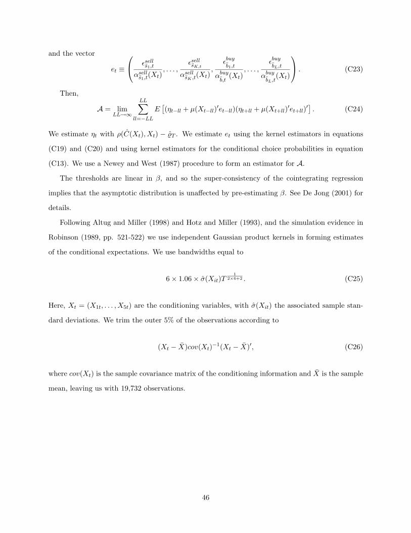
and the vector

et ≡ εsell

s1,t

αsells1,t(Xt)

, . . . ,εsellsK,t

αsellsK ,t(Xt)

,εbuy

b1,t

αbuy

b,t(Xt)

, . . . ,εbuy

bL,t

αbuy

bL,t(Xt)

. (C23)

Then,

A = limLL→∞

LL∑

ll=−LL

E[(ηt−ll + µ(Xt−ll)′et−ll)(ηt+ll + µ(Xt+ll)′et+ll)′

]. (C24)

We estimate ηt with ρ(C(Xt), Xt) − %T . We estimate et using the kernel estimators in equations

(C19) and (C20) and using kernel estimators for the conditional choice probabilities in equation

(C13). We use a Newey and West (1987) procedure to form an estimator for A.

The thresholds are linear in β, and so the super-consistency of the cointegrating regression

implies that the asymptotic distribution is unaffected by pre-estimating β. See De Jong (2001) for

details.

Following Altug and Miller (1998) and Hotz and Miller (1993), and the simulation evidence in

Robinson (1989, pp. 521-522) we use independent Gaussian product kernels in forming estimates

of the conditional expectations. We use bandwidths equal to

6× 1.06× σ(Xit)T1

2×6+2 . (C25)

Here, Xt = (X1t, . . . , X5t) are the conditioning variables, with σ(Xit) the associated sample stan-

dard deviations. We trim the outer 5% of the observations according to

(Xt − X)cov(Xt)−1(Xt − X)′, (C26)

where cov(Xt) is the sample covariance matrix of the conditioning information and X is the sample

mean, leaving us with 19,732 observations.

46

Table 1: Daily Trading Activity

The table reports summary statistics on the daily trading activity of Ericsson. The daily close-to-closereturns are calculated using the mid-quotes. The daily close-to-close returns for Ericsson shares traded onNASDAQ are calculated using daily data from the Center for Research in Security Prices. The number ofactive brokers per day is defined as the number of brokers who made at least one trade on a given tradingday.

Mean Std. Dev. Min. Max.

Daily closing mid-quote (Skr) 110.15 9.19 89.00 127.00Daily close-to-close return (percent) 0.21 3.04 −6.31 11.44Daily close-to-close return (percent) 0.10 2.45 −16.95 13.69on NASDAQ, January 2, 1989–December 31, 1993

Number of active brokers per day 19.28 2.28 14.00 23.00

Daily trading volume in millions of SKr

Stockholm Automated Exchange 38.77 19.53 11.58 114.88Internal crosses 12.20 9.04 1.48 57.51Block trades 0.39 0.92 0.00 5.45After-hours trades 4.66 6.15 0.00 28.26Total trading volume 56.02 29.52 13.06 201.28

Daily number of Stockholm Automated Exchange orders, 10:03 a.m.–2:30 p.m.

All orders 364.23 141.13 128 733Limit orders 212.18 77.58 73 408Market orders 152.04 67.14 55 330

47

Table 2: Order Submissions

The table reports descriptive statistics for the order submissions in Ericsson. The execution probability isdefined as the fraction of the order quantity that transacts within two trading days of the order submission.The time-to-fill is the number of minutes elapsed from the order submission until the order fills. When thereare multiple fills we weight each fill according to the fraction of the order quantity that is filled. Fills thatoccur later than two trading days after the order was submitted are ignored. The order quantity is measuredin 100’s of shares. There are 20,760 orders.

Order Number of orders Execution probability Time-to-fill Order quantityMean Mean Mean Std. Dev.

Buy orders

market 6031 1.00 0.00 19.72 39.211 tick limit 4225 0.68 24.55 25.14 37.602 tick limit 992 0.33 73.94 29.63 44.583 tick limit 893 0.12 172.33 14.65 32.38

Sell orders

market 4044 1.00 0.00 30.73 48.901 tick limit 3212 0.63 18.31 36.08 49.482 tick limit 800 0.28 84.21 37.08 44.873 tick limit 563 0.13 170.95 23.73 91.29

48

Table 3: Order Books

Descriptive statistics for the order books. The statistics in the table are computed for each order bookobserved in the market immediately prior to an order submission. There are 20,760 observations.

Mean Std.Dev. Min. Max.

Order quantities at quotes (100’s of shares)

3rd Ask 169.8 175.9 1.0 1061.12nd Ask 260.8 203.0 1.0 1161.01st Ask 200.9 194.1 1.0 1314.01st Bid 185.9 173.8 1.0 1504.22nd Bid 242.9 217.7 1.0 1504.23rd Bid 167.9 190.9 1.0 1355.2

Cumulative order quantities (100’s of shares)

1st+2nd+3rd Ask 631.5 368.8 13.0 1935.61st+2nd Ask 461.7 294.9 2.0 1809.01st+2nd Bid 428.8 310.2 5.0 2176.91st+2nd+3rd Bid 596.8 396.0 15.0 2730.4

Distance between price quotes (ticks)

bid-ask spread 1.1 0.3 1.0 6.03rd ask – 2nd ask 1.1 0.4 1.0 6.02nd ask – 1st ask 1.1 0.2 1.0 6.01st bid – 2nd bid 1.1 0.2 1.0 8.02nd bid – 3rd bid 1.1 0.5 1.0 10.0

49

Table 4: Description of the Conditioning Variables

The table describes how the construction of the conditioning variables. All variables are transformed to haveapproximately the same scale.

Conditioning variable Description

Order Quantity The number of shares in the order submitted at t.Transformed by taking the logarithm of the number of shares.

Ask Depth The number of shares in the order book at the best ask quote.Transformed by taking the logarithm of one plus the number of sharesdivided by 1000.

Bid Depth The number of shares in the order book at the best bid quote.Transformed by taking the logarithm of one plus the number of sharesdivided by 1000.

Lagged Volume The cumulative number of shares transacted during the minimum of theprevious ten minutes and the time since the market opening.Transformed by taking the logarithm of one plus the number of sharesdivided by 1000.

Index Volatility The standard deviation of the OMX index returns over the minimum of the60 minutes and the number of minutes since market opening.Transformed by taking the logarithm of one plus the volatility times

√270;

there are 270 trading minutes per day.

Time of Day The time since the market opening. Measured in seconds since midnight.Transformed by dividing by 3600.

50

Table 5: Test of Strictly Positive Conditional Choice Probabilities

The top panels of the table report the averages of the differences of the order choices and 0.02, multiplied bypositive instruments. Asymptotic standard errors in parentheses and p-values are reported below each pointestimate. The rightmost column and the bottom part of the table report joint MPC test statistics across theinstruments, the order prices, and across instruments and order prices, with p-values reported below eachtest statistic. We ensure that all instruments are strictly positive by replacing them with 0.00001 if they arezero.

Instruments JointOrder Order Ask Bid Lagged Index Time of MPC

Constant Quantity Depth Depth Volume Volatility Day statistic

Buy limit orders

1 tick 0.18 1.27 0.35 0.37 0.45 0.12 2.20 0.00(0.00) (0.03) (0.01) (0.01) (0.01) (0.00) (0.06) (0.00)1.00 1.00 1.00 1.00 1.00 1.00 1.00 0.99

2 ticks 0.03 0.20 0.04 0.04 0.07 0.02 0.32 0.00(0.00) (0.01) (0.00) (0.00) (0.01) (0.00) (0.02) (0.00)1.00 1.00 1.00 1.00 1.00 1.00 1.00 0.99

3 ticks 0.02 0.13 0.04 0.04 0.05 0.02 0.26 0.00(0.00) (0.01) (0.00) (0.00) (0.01) (0.00) (0.03) (0.00)1.00 1.00 1.00 1.00 1.00 1.00 1.00 0.99

Sell limit orders

1 tick 0.13 1.00 0.32 0.37 0.33 0.09 1.61 0.00(0.00) (0.03) (0.01) (0.01) (0.01) (0.00) (0.05) (0.00)1.00 1.00 1.00 1.00 1.00 1.00 1.00 0.99

2 ticks 0.02 0.15 0.03 0.04 0.05 0.01 0.21 0.00(0.00) (0.01) (0.00) (0.00) (0.01) (0.00) (0.02) (0.00)1.00 1.00 1.00 1.00 1.00 1.00 1.00 0.99

3 ticks 0.01 0.04 0.02 0.02 0.02 0.01 0.08 0.00(0.00) (0.01) (0.00) (0.00) (0.00) (0.00) (0.02) (0.00)1.00 1.00 1.00 1.00 1.00 1.00 1.00 0.99

Joint MPC statistic

All limit orders 0.00 0.00 0.00 0.00 0.00 0.00 0.00 0.000.98 0.99 0.98 0.98 0.98 0.99 0.98 1.00

51

Table 6: Monotonicity Tests for the Execution Probabilities

The top panels of the table report the average differences of the execution probability for different orderprices multiplied by positive instruments. The asymptotic standard errors in parentheses and p-values arereported below the point estimates. The rightmost column and the bottom part of the table report jointMDF test statistics across the instruments, the order prices, and across instruments and order prices, withp-values reported below each test statistic. We ensure that all instruments are strictly positive by replacingthem with 0.00001 if they are zero.

Instruments JointOrder Order Ask Bid Lagged Index Time of MPC

Constant Quantity Depth Depth Volume Volatility Day statistic

Buy limit orders

market 0.31 2.13 0.68 0.76 0.75 0.20 3.70 0.00- 1 tick limit (0.02) (0.11) (0.04) (0.04) (0.04) (0.01) (0.19)

1.00 1.00 1.00 1.00 1.00 1.00 1.00 0.99

1 tick limit 0.33 2.29 0.72 0.79 0.82 0.21 3.99 0.00- 2 tick limit (0.02) (0.16) (0.06) (0.05) (0.06) (0.02) (0.28)

1.00 1.00 1.00 1.00 1.00 1.00 1.00 0.99

2 tick limit 0.20 1.35 0.42 0.47 0.49 0.13 2.36 0.00- 3 tick limit (0.02) (0.16) (0.05) (0.05) (0.06) (0.02) (0.29)

1.00 1.00 1.00 1.00 1.00 1.00 1.00 0.99

Sell limit orders

market 0.35 2.44 0.77 0.85 0.86 0.22 4.23 0.00- 1 tick limit (0.02) (0.13) (0.05) (0.05) (0.05) (0.02) (0.20)

1.00 1.00 1.00 1.00 1.00 1.00 1.00 0.99

1 tick limit 0.35 2.37 0.77 0.85 0.85 0.22 4.17 0.00- 2 tick limit (0.02) (0.18) (0.06) (0.06) (0.07) (0.02) (0.28)

1.00 1.00 1.00 1.00 1.00 1.00 1.00 0.99

2 tick limit 0.13 0.92 0.28 0.32 0.33 0.09 1.60 0.00- 3 tick limit (0.03) (0.19) (0.06) (0.06) (0.08) (0.02) (0.29)

1.00 1.00 1.00 1.00 1.00 1.00 1.00 0.99

Joint MPC statistic

All limit orders 0.00 0.00 0.00 0.00 0.00 0.00 0.00 0.000.98 0.99 0.99 0.98 0.98 0.98 0.99 1.00

52

Table 7: Common Value Estimation

The first column reports unit root tests for the best bid quote, best ask quote, and the OMX index. Allseries are demeaned. There are 20,760 observations. The unit root test is an augmented Dickey-Fuller t-testwith 10 lags, and p-values are reported below each t-statistic. The second column reports the estimatedcoefficient on the demeaned OMX index using both quote series with the standard error in parentheses. Thefinal column reports an augmented Engle-Granger test for cointegration computed using 10 lags.

Cointegrating regressionUnit root test Coefficient Cointegration test

OMX index −0.89p-value = 0.79

Bid quote −1.11 0.37 − 3.67p-value = 0.71 (0.00) p-value < 0.03

Ask quote −1.08 0.36 − 3.62p-value = 0.72 (0.00) p-value < 0.03

53

Table 8: Monotonicity Tests for the Threshold Valuations

The top panels of the table report the average differences of threshold valuations for different order pricesmultiplied by positive instruments. Asymptotic standard errors in parentheses and the p-values are reportedbelow the point estimates. The rightmost column and the bottom part of the table report joint MDθ teststatistics across the instruments, the order prices, and across instruments and order prices, with p-valuesreported below each test statistic. We ensure that all instruments are strictly positive by replacing themwith 0.00001 if they are zero.

Threshold Instruments JointValuation Order Ask Bid Lagged Index Time of MPC

Difference Constant Quantity Depth Depth Volume Volatility Day statistic

Buy threshold valuations

θbuy(0, 1, Xt) 2.15 14.82 4.66 5.11 5.38 1.42 25.76 0.00−θbuy(1, 2, Xt) (0.15) (1.03) (0.37) (0.40) (0.40) (0.12) (1.84)

1.00 1.00 1.00 1.00 1.00 1.00 1.00 0.99

θbuy(1, 2, Xt) 1.21 8.34 2.73 3.02 2.93 0.78 14.58 0.00−θbuy(2, 3, Xt) (0.14) (0.93) (0.33) (0.35) (0.38) (0.12) (1.68)

1.00 1.00 1.00 1.00 1.00 1.00 1.00 0.99

Sell threshold valuations

θsell(1, 2, Xt) 2.02 13.89 4.58 5.06 5.02 1.32 24.28 0.00−θsell(0, 1, Xt) (0.16) (1.20) (0.38) (0.44) (0.44) (0.14) (1.83)

1.00 1.00 1.00 1.00 1.00 1.00 1.00 0.99

θsell(2, 3, Xt) 0.24 1.61 0.47 0.54 0.57 0.16 2.82 0.00−θsell(1, 2, Xt) (0.49) (3.61) (1.14) (1.29) (1.44) (0.41) (5.48)

0.69 0.67 0.66 0.66 0.65 0.65 0.70 0.99

Buy and sell threshold valuations

θbuy(2, 3, Xt) −1.43 −9.84 −3.26 −3.62 −3.47 −0.92 −17.27 13.16−θsell(2, 3, Xt) (0.42) (3.01) (1.00) (1.11) (1.25) (0.38) (4.77)

0.00 0.00 0.00 0.00 0.00 0.01 0.00 0.01

Joint MDθ statistic

Buy thresholds 0.00 0.00 0.00 0.00 0.00 0.00 0.00 0.000.75 0.76 0.74 0.75 0.75 0.76 0.75 1.00

Sell thresholds 0.00 0.00 0.00 0.00 0.00 0.00 0.00 0.000.75 0.75 0.75 0.75 0.75 0.75 0.75 1.00

Buy and sell 70.35 76.33 80.97 76.43 50.46 32.90 79.49 99.31thresholds 0.00 0.00 0.00 0.00 0.00 0.00 0.00 0.00

54

Table 9: Average Estimated Payoffs for Different Order Submissions

The table reports unconditional averages of the execution probabilities, the picking off risks, and estimatedpayoffs for traders with valuations equal to threshold valuations for the market and one tick, one tick andtwo tick, and two tick and three tick buy and sell orders. The estimated payoffs for traders with valuationsequal to the threshold valuations are computed by substituting estimates of the threshold valuations, theexecution probabilities, and the picking off risks, and the order quantity into equation (11), and dividing bythe order quantity. The order entry cost of c per share is set equal to zero. Asymptotic standard errors arereported in parentheses, and are computed using 50 lags.

Order Execution Picking off Estimated payoff atprobability risk threshold valuation

Buy orders

1 tick limit 0.68 0.01 1.94(0.01) (0.03) (0.13)

2 tick limit 0.33 −0.09 0.39(0.02) (0.05) (0.06)

3 tick limit 0.12 −0.15 −0.02(0.02) (0.10) (0.05)

Sell orders

1 tick limit 0.63 0.01 1.54(0.01) (0.02) (0.10)

2 tick limit 0.27 0.14 0.19(0.02) (0.07) (0.09)

3 tick limit 0.13 0.11 0.12(0.02) (0.08) (0.16)

55

Figure 1: Survivor Functions

The top graph plots the survivor function for limit orders. The survivor function at any time isdefined as the probability that a limit order is outstanding a given number of minutes after it wassubmitted. The middle and the bottom graphs plot the cumulative distribution functions for thelimit order execution and cancellation times. All three functions are computed for orders submittedbetween 10:03 a.m. and 2:30 p.m. There are a total of 11,760 limit orders submitted. The survivorand distribution functions are calculated by assigning a weight to each observation equal to thefraction of the order quantity executed or canceled. Limit orders submitted during the last twotrading days in our sample are not used in the calculations.

0 60 120 180 240 300 3600

0.1

0.2

0.3

0.4

0.5

0.6

0.7

0.8

0.9

1Survivor Function of Limit Orders

time (minutes after order submission)

Sur

vivo

r F

unct

ion

0 60 120 180 240 300 3600

0.1

0.2

0.3

0.4

0.5

0.6

0.7

0.8

0.9

1Cumulative Distribution of Limit Order Execution Time

time (minutes after order submission)

Pro

b(tim

e(ex

ecut

ion)

≤ ti

me)

0 60 120 180 240 300 3600

0.1

0.2

0.3

0.4

0.5

0.6

0.7

0.8

0.9

1Cumulative Distribution of Limit Order Cancellation Time

time (minutes after order submission)

Pro

b(tim

e(ca

ncel

) ≤

time)

56

Figure 2: Indirect Utility Function

The graph provides an example of the indirect utility function. The order quantity is set equal toone. The horizontal axis is the trader’s valuation, and the vertical axis is the expected payoff fromalternative order submissions. Sell orders are plotted with dashed lines (- - -) and buy orders areplotted with dashed-dotted lines (-.-.). The indirect utility function is plotted with the dark solidline (—).

θsellt

(0,1,1) θsellt

(1,2,1) θsellt

(2,NO,1)

θt(2,2,1)

θbuyt

(2,NO,1) θbuyt

(1,2,1) θbuyt

(0,1,1)

Valuation vt=y

t+u

0

Expected

Payoff

← Et[U

t,t+ϒ | dbuy

t,0=1,u

t,1]

← Et[U

t,t+ϒ | dbuy

t,1=1,u

t,1]

← Et[U

t,t+ϒ | dbuy

t,2=1,u

t,1]

Et[U

t,t+ϒ | dsell

t,0=1,u

t,1] →

Et[U

t,t+ϒ | dsell

t,1=1,u

t,1] →

Et[U

t,t+ϒ | dsell

t,2=1,u

t,1] →

← Vt(y

t+u,1)

57

Figure 3: Optimal Order Submission Strategy

The graph illustrates an example of the optimal order submission strategy. The probabilities of ob-serving different order submissions are determined by the threshold valuations and the distributionof private valuations. The threshold valuations are computed using equations (16) through (19).The distribution of the private valuations Gt is a mixture of three normal distributions.

θsellt

(0,1,1)−yt

|

θsellt

(1,2,1)−yt

|

θsellt

(2,NO,1)−yt

|

θbuyt

(2,NO,1)−yt

|

θbuyt

(1,2,1)−yt

|

θbuyt

(0,1,1)−yt

|

Private Valuation u

0

0.1

0.2

0.3

0.4

0.5

0.6

0.7

0.8

0.9

1

Gt(u

)=P

rob(

u t ≤ u

)

Prob(buy market)

Prob(1 tick buy limit)

Prob(2 tick buy limit)

No Order

Prob(2 tick sell limit)

Prob(1 tick sell limit)

Prob(sell market)

58

Figure 4: Example of Violation of the Monotonicity of the Thresholds

The figure illustrates an example where the threshold valuations do not satisfy the monotonicitycondition: θbuy

t (0, 1, 1) < θbuyt (1, 2, 1). The execution probabilities for limit orders are monotonically

decreasing in the distance between the limit order price and the best ask quote. The executionprobabilities are ψbuy

t (0, 1) = 1, ψbuyt (1, 1) = 0.7, ψbuy

t (2, 1) = 0.6; the tick size is 1; the best askquote is 100; and the picking off risks are equal to zero. The indirect utilities for a trader submittinga buy market order (- - -), a one tick buy limit order (—), and a two tick buy limit order(-.-.) areplotted as a function of the trader’s valuation.

θbuyt

(0,1,1) θbuyt

(1,2,1)

Valuation vt=y

t+u

98 99 100 101 102 103 104 105 1060

1

2

3

4

5

Et[U

t,t+ϒ | dbuy

t,0=1,u

t,1] → .

← Et[U

t,t+ϒ | dbuy

t,1=1,u

t,1]

Et[U

t,t+ϒ | dbuy

t,2=1,u

t,1] → .

Exp

ecte

d P

ayof

f

59

Figure 5: Estimated Payoffs

The figure plots the estimated payoffs as a function of the trader’s valuation. The estimated payoffsare evaluated at the sample observation with conditioning variables closest to their sample averages.The horizontal axis gives the trader’s valuation and the vertical axis the payoffs for alternative ordersubmissions.

113 114 115 116 117 118 119 120−0.5

0

0.5

1

1.5

2

2.5

3

3.5

Exp

ecte

d P

ayof

f

Valuation v=yt+u

Sell Orders

Et[U

t,t+ϒ | dsell

t,0=1,u

t,1]

Et[U

t,t+ϒ | dsell

t,1=1,u

t,1]

Et[U

t,t+ϒ | dsell

t,2=1,u

t,1]

Et[U

t,t+ϒ | dsell

t,3=1,u

t,1]

113 114 115 116 117 118 119 120−0.5

0

0.5

1

1.5

2

2.5

3

3.5

Exp

ecte

d P

ayof

f

Valuation v=yt+u

Buy Orders

Et[U

t,t+ϒ | dbuy

t,0=1,u

t,1]

Et[U

t,t+ϒ | dbuy

t,1=1,u

t,1]

Et[U

t,t+ϒ | dbuy

t,2=1,u

t,1]

Et[U

t,t+ϒ | dbuy

t,3=1,u

t,1]

60