Physikalisches Praktikum für Fortgeschrittene (P3)

Elektrische Leitfähigkeit von Festkörpern bei

tiefen Temperaturen

Betreuer: Dr. Lukashenko

Michael Lohse, Matthias Ernst

Gruppe 11

Karlsruhe, 8.11.2010

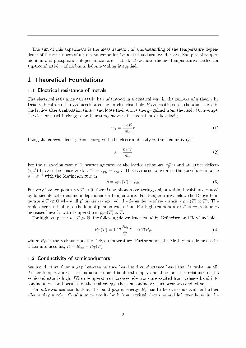
The aim of this experiment is the measurement and understanding of the temperature depen-dence of the resistances of metals, superconductive metals and semiconductors. Samples of copper,niobium and phosphorous-doped silicon are studied. To achieve the low temperatures needed forsuperconductivity of niobium, helium-cooling is applied.

1 Theoretical Foundations

1.1 Electrical resistance of metals

The electrical resistance can easily be understood in a classical way in the context of a theory byDrude. Electrons that are accelerated by an electrical eld E are scattered at the atom cores inthe lattice after a relaxation time τ and loose their entire energy gained from the eld. On average,the electrons (with charge e and mass me move with a constant drift velocity

vD =−eEme

τ (1)

Using the current density j = −envD with the electron density n, the conductivity is

σ =ne2τ

me(2)

For the relaxation rate τ−1, scattering rates at the lattice (phonons, τ−1Ph ) and at lattice defects

(τ−1St ) have to be considered: τ−1 = τ−1

Ph + τ−1St . This can used to express the specic resistance

ρ = σ−1 with the Mathiesen rule asρ = ρPh(T ) + ρSt (3)

For very low temperatures T → 0, there is no phonon scattering, only a residual resistance causedby lattice defects remains independent on temperature. For temperatures below the Debye tem-perature T Θ where all phonons are excited, the dependence of resistance is ρPh(T ) ∝ T 5. Therapid decrease is due to the loss of phonon excitation. For high temperatures T Θ, resistanceincreases linearly with temperature: ρPh(T ) ∝ T .For high temperatures T Θ, the following dependence found by Grüneisen and Borelius holds:

RT(T ) = 1.17RΘ

ΘT − 0.17RΘ (4)

where RΘ is the resistance at the Debye temperature. Furthermore, the Mathiesen rule has to betaken into account, R = Rres +RT(T ).

1.2 Conductivity of semiconductors

Semiconducturs show a gap between valence band and conductance band that is rather small.At low temperatures, the conductance band is almost empty and therefore the resistance of thesemiconductor is high. When temperature increases, electrons are excited from valence band intoconductance band because of thermal energy, the semiconductor thus becomes conductive.For intrinsic semiconductors, the band gap of energy Eg has to be overcome and no further

eects play a role. Conductance results both from excited electrons and left-over holes in the

2

valence band. In total, conductivity and resistance of intrinsic semiconductors at temperature Tcan be expressed as

σi = Cie− Eg

2kT

R = RmineEg2kT

(5)

with the Boltzmann constant k and material-dependent constants Ci and Rmin.In constrast, extrinsic semiconductors show a more complicated behaviour because here, the

seminconductor is doped with other atoms with more or less electrons, acting as electron donators(n-doped semiconductors) or acceptors (p-doped semiconductors). This is particular important atlow temperatures, where conductance is signicantly larger than with intrinsic semiconductors. Athigh temperatures, eects of thermal excitation become more important and thus, extrinsic andintrinsic semiconductors show the same behaviour in high-temperature limes. The full temperaturedependence of extrinsic semiconductors is rather complicated, as it consists of several parts thatplay a main role in a certain temperature range each. A sample can be found in the preparationfolder (g. 2, page 14f).

1.3 Superconductivity

Some materials show a sharp drop in their electrical resistance to zero below a certain criticaltemperature Tc. This phenomenon is called superconductivity and was discovered experimentallymore than 100 years ago. Because of this sharp transition, it can be considered as phase transition,expressed by an order parameter of the eletrons. Critical temperatures for metallic superconductorsare around 0 − 10K. Other superconductors with more complicated structures like YBaCo showcritical temperatures up to 150K.

1.4 BCS-theory

An explanation for superconductivity has been given by Bardeen, Cooper and Schrieer (BCS-theory). Electrons moving through an atomar lattice can polarize this lattice. The polarizationcan now act on another electron, thus creating a correlation between these two electrons that isattrative and larger than their Coulombic repulsion. This correlation is transmitted by phononsand is called Cooper pair. A Cooper pair consists of two electrons of opposite spin, (~p ↑,−~p ↓).In total, it has a spin of 0 and is therefore a boson. Unlike fermions (as electrons), several bosonscan be in the same state, mainly the ground state. In the BCS theory, a close correlation betweenall cooper pairs is postulated, they have to be in the same quantum mechanical state. Because ofthis, interaction like momentum transfer can not act on a single Cooper pair but has to act on allCooper pairs at once. Because this is impossible, electrons can not exchange momentum with thelattice, so there is no resistance of the electric current in a superconductor.To break a Cooper pair, the according energy of the correlation is needed. This energy can

either be thermal energy that increases the momentum of all cooper pairs so they nally collapseor can be supplied by a magnetic eld. If a magnetic eld is applied to a superconductor, acurrent is induced. Unlike in usual conductors, where this current weakens very fast because ofthe resistance of the conductor, the induced current in a superconductors stays permanent as theresistance vanishes. Furthermore, the induced current creates an internal magnetic eld that hasthe same absolute value as the external so it cancels this inside of the superconductor except fora thin layer of thickness λ on the surface. This phenomenon is called Meissner eect (in germanMeiÿner-Ochsenfeld Eekt). When the external magnetic eld reaches a certain value, the Meissner

3

eect breakes down (of course, the critical magnetic eld also depends on temperature). Becauseof the Meissner eect, a superconductor can be considered as perfect diamagnet, so the magneticsusceptibility vanishes,

χ =µ0M

B= −1 (6)

with the magnetization M , the magnetic eld B and the vacuum permeability µ0. Superconduc-tors with a critical magnetic eld at which superconductivity collapses at once and the Meissnereect no longer holds are called type I superconductors. Some superconductors, termed type IIsuperconductors show a dierent behaviour. At low temperatures, the Meissner eect can be ob-served. At a lower critical eld Bc1, they enter a state called Shubnikov phase where the magneticeld is not repelled completely from the inside of the superconductor but enter it in so called vor-tices. This gradually weakens superconductivity until a second critical magnetic eld Bc1 where itcollapses.

1.5 GLAG-theory

A phenomenological treatment of superconductivity has been given by Ginsburg, Landau, Abri-kosov and Gorkov (GLAG-theory). Two characteristic lengths are crucial: the penetration depthλ, where the magnetic eld has dropped to the fraction of 1

e of its outer value found to be

λ(T ) = λ(0)

(1−

(T

Tc

)4)− 1

2

(7)

and the Ginsburg Landau coherence length, describing thermodynamic uctuations of the cooperpairs is determined as

ξGL(T ) =ξ

(0)GL√

1− TTc

(8)

The coherence length at T = 0K is given by

ξ(0)GL =

( −Φ0

2πSTc

) 12

(9)

with the ux quantum Φ0 = 2−07 ·10−15V s and the slope S = dBc2dT

∣∣∣T=Tc

of the critical magnetic

eld Bc2

Bc2(T ) =Φ0

2πξ2GL(T )

=Φ0

2πξ(0)GL

2

(1− T

Tc

)

⇒ S =dBc2

dT

∣∣∣∣T=Tc

=−Φ0

2πξ(0)GL

2Tc

(10)

With the Ginsburg Landau parameter κ = λξGL

, superconductors can be classied. For type I

superconductors, κ is found to be κ < 1√2, for type II superconductors κ > 1√

2. Niobium which

we will use as sample is just at the border of those two types, depending on the number of latticedefects.

4

2 Experimental Setup

All measurements are carried out in a cryostat, shown in gure 4 of the preparation folder. Thiscryostat consists of two double-walled glass dewars. The outer dewar is lled with liquid nitrogen,thus able to cool the samples down to at most 77K. The inner dewar is then lled with liquidhelium, so the samples can be cooled to at most 4K and superconductivity of the niobium samplecan be reached. Inside of the inner dewar, a sample holder and a heater are attached. The sampleholder is sourrounded by a superconductive coil, for a normal conducting coil would vapour theliquid helium because of the Joule heat in a short time.Temperature can be taken via a platinum sensor that is able to properly measure temperature

down to about 50K because of the mainly linear dependece of resistance on current and a car-bon sensor, for which resistance increases at lower temperatures thus enabling us to gauge lowtemperatures accurately.Three samples are to be measured: a copper sample as metal, a phosphorus-doped silicon sample

as a semi-conductor and a niobium sample. We expect these interdependece of the resistance ontemperature:

• Copper sample: Copper is a typical metal, so we expect a linearity at high temperatures. Atabout the Debye temperature, we expect a proportionality of R ∝ T 5. At lower temperatures,this should turn into a constant, the residual resistance.

• Silicon sample: Phosphorus-doped silicon is a semiconductor. We therefore expect an inverseexponential correlation of resistance and temperature, so the resistance at low temperaturesought to be very high.

• Niobium sample: Niobium is a metal which becomes superconductive at TC = 9.2K. Wecan observe this transition because of the helium cooling, so we expect a similar shape as forcopper, except for a drop from the residual resistance to R = 0Ω at about that temperature.

3 Procedure

After we had been introduced to the experimental setup by the supervisor, we evacuated the innerdewar and its walls to avoid water residues, then relled the walls with a small amount of heliumand ushed the inner dewar with helium. We then lled the outer dewar with liquid nitrogen tocool down the samples.We began taking data at about 4,5C. Unfortunately, we forgot to measure the resistances of

the samples and thermometers at room temperature. The highest values we measured seemed tobe in reasonable agreement to the values in the preparation folder. Furthermore, we have beenable to extrapolate most of these values because of the expected and observed linear dependenceof resistance on temperature. Doing this, we obtain RCu = 2.43Ω, RNb = 50.82Ω, RSi = 0.09Ωand RPt = 109.54Ω. These are a little bit dierent from the values provided in the preparationfolder, but not very much.At about 200K, we poured liquid helium to the inner dewar to speed up the cooling process.

Because the temperature dropped so fast, we could not write down the values as before but we wereable to take pictures of the displays from which we gained proper values of this fast cool-down. Atabout 55K, we switched from platinum to carbon sensor for proper temperature measurement.To determine the dependence of the critical temperature on the magnetic eld, we used a plotting

device to gain the resistance-temperature-curve for dierent magnetic elds. We increased the

5

current through the superconductive coil from 0A to 12A in steps of 1.5A. Each time, we heatedthe sample so it lost superconductivity and plotted the cool-down curve. We noticed a lineardecrease of resistance on increasing magnetic eld as expected.Finally, we used the heater to slowly increase temperature of the samples to about 150K an took

resistance values again to gain more accurate data in that domain.

4 Analysis

The values we measured for the resistance curves are the voltages that dropped on each sample byproviding each one with a current of I = 1mA. The resistance is then easily computed via R = U

I .

4.0.1 Some words on error calculation

In principle, we would have to to error propagation and thereby calculate systematical and statis-tical errors of all values we measured. Unfortunately, the manual did not dene any errors of themeasuring units. In particular, we don't know anything about the errors in the thermal sensorswe are using and the tted functions supplied in the manual that we have to use to compute thetemperature are also mainly given without any error estimates. So we could only guess systemat-ical errors in our experiment but as we do not know the experimental setup and its capabilitiesvery well, we do not want to speculate on numbers and so a specication of systematical errorsis impossible. It seems though that systematical errors are quite small or being compensated asmost of our results appear quite reasonable.In course of the many linear regressions we performed, statistical errors have been obtained as

well. We will declare those with the values of the ts but we will not perform any error propagationas this is only part of the entire error and we can not do error calculation on systematical errorsas just explained.

4.1 Resistance graphs

Figure 1 shows the resistance graph for the three samples we measured. As one can clearly see,Niobium has a rather high resistance that decreases with decreasing temperature and drops tozero at about 5K. Copper has a quite low resistance that steadily decreases and the Si:P sampleshows a very low resistance at high temperatures but with a sharp increase at about 4K.To investigate the shapes of the resistance curves in more detail, these are shown in a single grapheach.Figure 2 shows our results for the copper sample. The linear dependence of the resistance on the

temperature from room temperature to about 55K can clearly be seen. The slightly bent shape(red) of the cool down curve between 55K and 200K is due to the addition of liquid helium. Thisconsiderably speeded up the cool-down process so our measurements obviously did not take placein thermal equilibrium. Later, when whe heated the samples more slowly and took the valuesagain, the linear developing of the values is much better (yellow curve). At lower temperaturesthan about 50K, the linearity changes to a more curved shape and becomes constant at about30K. To analyze the domain of low temperatures, the range between 0K and 70K is depicted ingure 3.

6

0

0.05

0.1

0.15

0.2

0.25

0 10 20 30 40 50 60 70

Resistance

[Ω]

Temperature [K]

Cool down, Pt sensorCool down, C sensorWarm up, C sensorWarm up, Pt sensor

Figure 3: Resistance graph of Copper sample at lower temperatures

0

10

20

30

40

50

0 50 100 150 200 250 300

Resistance

[Ω]

Temperature [K]

Si sampleCu sampleNb sample

Figure 1: Resistance graph of all measured samples

0

0.5

1

1.5

2

2.5

0 50 100 150 200 250 300

Resistance

[Ω]

Temperature [K]

Cool down, Pt sensorCool down, C sensorWarm up, C sensorWarm up, Pt sensor

Figure 2: Resistance graph of Copper sample

7

There, the non-linear behavior within a certain range (this will be discussed later) and the lowbut nevertheless non-vanishing residual resistance can be seen.The graph of the niobium sample is shown in gure 4.

0

10

20

30

40

50

0 50 100 150 200 250 300

Resistance

[Ω]

Temperature [K]

Cool down, Pt sensorCool down, C sensorWarm up, C sensorWarm up, Pt sensor

Figure 4: Resistance graph of Niobium sample

Despite the overall higher resistance of niobium, the associated curve resembles the one of thecopper sample except at very low temperatures. There, the transition to the superconductive statewith a vanishing resistance is obious. For niobium, too, the low temperature domin are upscaledand shown in gure 5.

20

21

22

23

24

25

26

0 10 20 30 40 50 60 70

Resistance

[Ω]

Temperature [K]

Cool down, Pt sensorCool down, C sensorWarm up, C sensorWarm up, Pt sensor

Figure 5: Resistance graph of Niobium sample at lower temperatures

Note that the transition to the superconductive state is not shown. Here, too, we see the residualresistance before this transition and the non-linear behavior.Finally, the graph of the silicon sample is shown in gure 6. The scaling is logarithmic on both

axes.

8

0.01

0.1

1

10

100

10 100

Resistance

[Ω]

Temperature [K]

Cool down, Pt sensorCool down, C sensorWarm up, C sensorWarm up, Pt sensor

Figure 6: Resistance graph of Phosphorous doped Silicon sample

For silicon, a very dierent shape than ones of the metallic samples has to be stated. Asalready pointed out and in agreement to our expectation, the resistance of silicon increases almostimperceptibly with decreasing temperature and then sharply increases. This behaviour results inthe semiconducting nature of silicon.

4.2 Debye temperatures and power of non-linear temperature-resistancedependence

To obtain the Debye temperature Θ and the Debye resistance R(Θ), we use the Grüneisen-Borrelius-equation:

RT (T ) = 1.17RΘ

ΘT − 0.17RΘ (11)

As the Matthiesen rule holds, R = Rres +RT (T ), we have to subtract the residual resistance fromthe measured values to get the correct results.

RT (T ) = 1.17RΘ

Θ︸ ︷︷ ︸m

T −0.17RΘ +Rres︸ ︷︷ ︸c

(12)

Then, we can perform a linear regression and use the values the axis intercept c and for the slopem to gain the values of interest by RΘ = (Rres − c)/0.17 and Θ = 1.17RΘ/m.The residual resistances were taken from the lowest values we measured. For the copper sample,

these remained constant at Rres,Cu = 0.02Ω from 22K to 7K. For niobium, we used the last valuemeasured before the transition to superconductivity, so Rres,Nb = 21.23Ω.The linear regression graph for copper is displayed in picture 7.

9

-0.5

0

0.5

1

1.5

2

2.5

0 50 100 150 200 250 300

Resistance

[Ω]

Temperature [K]

Measured valuesLinear regression

Figure 7: Linear regression of copper at higher temperatures

We used the values during cooling down before we added helium and the values during warming-up from 70K upwards, where our data suited the suggested linearity very well. This corresponds tothe values for m = (0.009114± 0.000017)Ω/K and c = (−0.4304± 0.0033Ω). We therefore obtain

Θ = 340.12K

RΘ = 2.65Ω(13)

The very small statistical errors of these values can be neglected as the instrumental error isassumed to be much larger. Nevertheless, our results is in surprising agreement to published dataof Θ = 343.5K (C. Kittel, Introduction to Solid State Physics, 7th Ed., Wiley, 1996).With the same procedure, we can calculate Θ and RΘ for niobium. The linear regression graph

is supplied in g. 8.

0

10

20

30

40

50

60

0 50 100 150 200 250 300

Resistance

[Ω]

Temperature [K]

Measured valuesLinear regression

Figure 8: Linear regression of niobium at higher temperatures

10

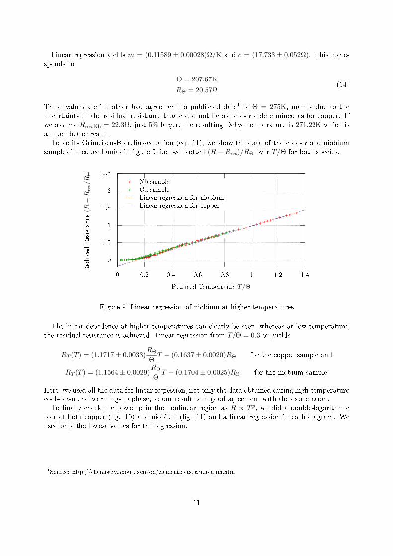
Linear regression yields m = (0.11589 ± 0.00028)Ω/K and c = (17.733 ± 0.052Ω). This corre-sponds to

Θ = 207.67K

RΘ = 20.57Ω(14)

These values are in rather bad agreement to published data1 of Θ = 275K, mainly due to theuncertainty in the residual resistance that could not be as properly determined as for copper. Ifwe assume Rres,Nb = 22.3Ω, just 5% larger, the resulting Debye temperature is 271.22K which isa much better result.To verify Grüneisen-Borrelius-equation (eq. 11), we show the data of the copper and niobium

samples in reduced units in gure 9, i.e. we plotted (R−Rres)/RΘ over T/Θ for both species.

0

0.5

1

1.5

2

2.5

0 0.2 0.4 0.6 0.8 1 1.2 1.4

ReducedResistance

(R−

Rre

s/R

Θ]

Reduced Temperature T/Θ

Nb sampleCu sampleLinear regression for niobiumLinear regression for copper

Figure 9: Linear regression of niobium at higher temperatures

The linear depedence at higher temperatures can clearly be seen, whereas at low temperature,the residual resistance is achieved. Linear regression from T/Θ = 0.3 on yields

RT (T ) = (1.1717± 0.0033)RΘ

ΘT − (0.1637± 0.0020)RΘ for the copper sample and

RT (T ) = (1.1564± 0.0029)RΘ

ΘT − (0.1704± 0.0025)RΘ for the niobium sample.

Here, we used all the data for linear regression, not only the data obtained during high-temperaturecool-down and warming-up phase, so our result is in good agreement with the expectation.To nally check the power p in the nonlinear region as R ∝ T p, we did a double-logarithmic

plot of both copper (g. 10) and niobium (g. 11) and a linear regression in each diagram. Weused only the lowest values for the regression.

1Source: http://chemistry.about.com/od/elementfacts/a/niobium.htm

11

-6

-4

-2

0

2

4

6

3 3.5 4 4.5 5 5.5 6

Log.Resistance

ln((R−

Rres)/

Ω)

Log. Temperature ln(T/K)

Measured values

Linear regression

Figure 10: Double-logarithmic graph for copper

-6

-4

-2

0

2

4

6

8

10

12

2 2.5 3 3.5 4 4.5 5 5.5 6

Log.Resistance

ln((R−R

res)/

Ω)

Log. Temperature ln(T/K)

Measured values

Linear regression

Figure 11: Double-logarithmic graph for niobium

We get pCu = 4.65 ± 0.93 and pCu = 3.97 ± 0.43. In both cases, we do not have enough datain the non-linear region and those we have are widely scattered, so the t is based on very fewpoints. This explains the dierence from the expected power pex = 5.

4.3 Specic resistances and mean free paths

To calculate the specic resistances of our copper and niobium samples, we use the denition ofthe specic resistance ρ:

ρ(T ) = R(T )A

l(15)

with the electrical resistance R, the cross section A and the lenght l of the sample under consid-eration. If we assume the dimensions of the samples to be independent on temperature, we can

12

calculate those with the values given in the preparation folder and then calculate the specic resis-tance at low temperatures using the residual resistances determined above. Knowing the specicresistance, the mean free path ` can be calculated via ` = ρ`

ρ with the values of ρ` given in themanual.For the copper sample, the following values are given in the preparation folder:

ρCu(300K) = 1.71 · 10−8Ω cm ρ` = 658.7 · 10−18Ωm2

d = 1 · 10−4m⇒ ACu = π

(d

2

)2

= 7.85 · 10−9m2

To calculate the resistance of copper at 300K, we use the Grüneisen-Borrelius-equation 12 withthe values we found above, ΘCu = 340.12K, RΘ,Cu = 2.65Ω (see eq. 13) and Rres,Cu = 0.02Ω.We obtain R(300K) = 2.30Ω and, with equation 15, lCu = RA

ρ = 1.06m. Using the residualresistance and the assumption of temperature-independent sample volume, we get ρCu(4.2K) =1.48 · 10−10Ω m. The mean free path at T = 4.2K is then

`Cu,4.2K =ρ`

ρ=

658.7 · 10−18Ωm2

1.48 · 10−10Ω m= 4.44 · 10−6Ω = 4.44µΩ (16)

This rather high value compared to atomar dimension shows us that at this low temperature, theatoms are mainly "frozen" so collisions of electrons with atoms are much less probable than atroom temperature so the mean free path is rather long.For niobium, we can nd the following values in the preparation folder:

ρ` = 375 · 10−18Ωm2 l = 8 · 10−3m

w = 9 · 10−4m s = 40 · 10−9m ⇒ ANb = w · s = 3.60 · 10−11m2

As the length is given, we only need to calculate the specic resistance ρNb(12K) = 9.55 ·10−8Ωm.Using this, we get

`Nb,12K = 3.93 · 10−9m = 3.93nm (17)

This value is much smaller than the one found for copper (corresponding to the much higherresidual resistance). We see that the transition to superconductivity that occurs only 3Kbelowand where the mean free path is innity requires an abrupt phase transition.

4.4 Superconductivity of Niobium

Now, we want to determine the temperature dependency of the upper critical magnetic eldBc2. As described above, we used the supplied device which plotted the voltage that droppedon the niobium sample. After we had calibrated the device, we disabled the plotter, heated thesample so it lost superconductivity, reenabled the plotter and let the sample cool down belowthe critical temperature. We did that several times, where we increased the current through thesuperconducting coil from 0A to 12A in steps of 1.5A.In the plots, we could not see a very sharp transition but rather a smoothed shape. We thereforeused the points where the voltage had dropped to the half of its initial value to calculate the criticaltemperatures. The magnetic eld is computed by the formula given in the manual,

B = µ0n

2lI

(x+ l/2√

r2 + (x+ l/2)2− x− l/2√

r2 + (x− l/2)2

)(18)

13

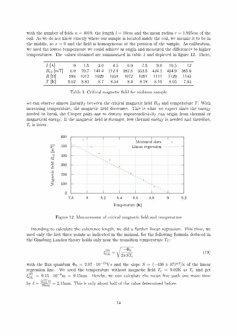
with the number of folds n = 4019, the length l = 10cm and the mean radius r = 1.925cm of thecoil. As we do not know exactly where our sample is located inside the coil, we assume it to be inthe middle, so x = 0 and the eld is homogeneous at the position of the sample. As calibration,we used the lowest temperature we could achieve as origin and measured the dierences to highertemperatures. The values obtained are summarized in table 1 and depicted in gure 12. There,

I [A] 0 1.5 3.0 4.5 6.0 7.5 9.0 10.5 12Bc2 [mT] 0.0 70.7 141.4 212.1 282.8 353.5 424.2 494.9 565.6R [Ω] 988 1012 1029 1051 1072 1091 1111 1129 1145T [K] 9.02 8.83 8.7 8.54 8.4 8.28 8.15 8.05 7.95

Table 1: Critical magnetic eld for niobium sample

we can observe almost linearity between the critical magnetic eld Bc2 and temperature T . Withincreasing temperature, the magnetic eld decreases. This is what we expect since the energyneeded to break the Cooper pairs ans so destroy supercondictivity can origin from thermal ormagnetical energy. If the magnetic eld is stronger, less thermal energy is needed and therefore,Tc is lower.

0

100

200

300

400

500

600

7.8 8 8.2 8.4 8.6 8.8 9 9.2

Magnetic

eldB

c2[m

T]

Temperature [K]

Measured dataLinear regression

Figure 12: Measurement of critical magnetic eld and temperature

Intending to calculate the coherence length, we did a further linear regression. This time, weused only the last three points as indicated in the manual, for the following formula deduced inthe Ginsburg Landau theory holds only near the transition temperature TC:

ξ(0)GL =

√−Φ0

2πSTc(19)

with the ux quantum Φ0 = 2.07 · 10−15V s and the slope S = (−436 ± 47)mT/K of the linearregression line. We used the temperature without magnetic eld Tc = 9.02K as Tc and get

ξ(0)GL = 9.15 · 10−9m = 9.15nm. Hereby, we can calculate the mean free path one more time

by ` =(ξ

(0)GL)2

39nm = 2.15nm. This is only about half of the value determined before.

14

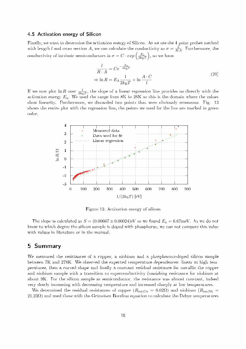
4.5 Activation energy of Silicon

Finally, we want to determine the activation energy of Silicon. As we use the 4-point probes methodwith length l and cross section A, we can calculate the conductivity as σ = L

R·A . Furthermore, the

conductivity of intrinsic semiconductors is σ = C · exp(

Ea2kBT

), so we have

l

R ·A = Ce− Ea

2kBT

⇒ lnR = EA1

2kBT+ ln

A · Cl

(20)

If we now plot lnR over 12kBT

, the slope of a linear regression line provides us directly with theactivation energy Ea. We used the range from 8K to 28K as this is the domain where the valuesshow linearity. Furthermore, we discarded two points that were obviously erroneous. Fig. 13shows the entire plot with the regression line, the points we used for the line are marked in greencolor.

-3

-2

-1

0

1

2

3

4

0 100 200 300 400 500 600 700 800 900

lnR/Ω

1/(2kBT ) [eV]

Measured dataData used for tLinear regression

Figure 13: Activation energy of silicon

The slope is calculated as S = (0.00667± 0.00024)eV so we found Ea = 6.67meV. As we do notknow to which degree the silicon sample is doped with phosphorus, we can not compare this valuewith values in literature or in the manual.

5 Summary

We measured the resistances of a copper, a niobium and a phosphorous-doped silicon samplebetween 7K and 278K. We observed the expected temperature dependences: linear at high tem-peratures, then a curved shape and nally a constant residual resistance for metallic the copperand niobium sample with a transition to superconductivity (vanishing resistance for niobium atabout 9K. For the silicon sample as semiconductor, the resistance was almost constant, indeedvery slowly increasing with decreasing temperature and increased sharply at low temperatures.We determined the residual resistances of copper (Rres,Cu = 0.02Ω) and niobium (Rres,Nb =

21.23Ω) and used these with the Grüneisen-Borelius-equation to calculate the Debye temperatures

15

and resistances. These are ΘCu = 340.12K, RΘ,Cu = 2.65Ω, ΘNb = 207.67K and RΘ,Nb = 20.57Ω.We could verify the Grüneisen-Borelius-equation and found the powers of R ∝ T p in the to bepCu = 4.65 and pCu = 3.97.To obtain the mean free paths of the copper and niobium samples, we rst calculated the specic

resistances of copper ρCu(4.2K) = 1.48 · 10−10Ωm and niobium ρNb(12K) = 9.55 · 10−8Ωm. Themean free paths are `Cu,4.2K = 4.44µm and `Nb,12K = 3.93nm.Further, we applied a magnetic eld to the niobium sample to calculate the Ginsburg-Landau

coherence length. We got ξ(0)GL = 9.15nm. Using this value, we could calculate the mean free path

of niobium again, resulting in ` == 2.15nm. This is in the same range of magnitude but onlyalmost half of the value obtained in the rst place.Finally, we calculated the activation energy of silicon by using the exponential dependence of

the conductance on this energy: Ea = 6.67meV.

Appendix

• Graph of resistance on temperature for dierent magnetic elds and copy (2 sheets)

• Measurement data

16