Electronic Structure forElectronic Structure forExcited StatesExcited States

((multiconfigurationalmulticonfigurationalmethods)methods)

Spiridoula MatsikaSpiridoula Matsika

Excited Electronic StatesExcited Electronic States• Theoretical treatment of excited states is needed

for:– UV/Vis electronic spectroscopy– Photochemistry– Photophysics

• Electronic structure methods for excited statesare more challenging and not at the same stageof advancement as ground state methods– Need balanced treatment of more than one states

that may be very different in character– The problem becomes even more complicated when

moving away from the ground state equilibriumgeometry

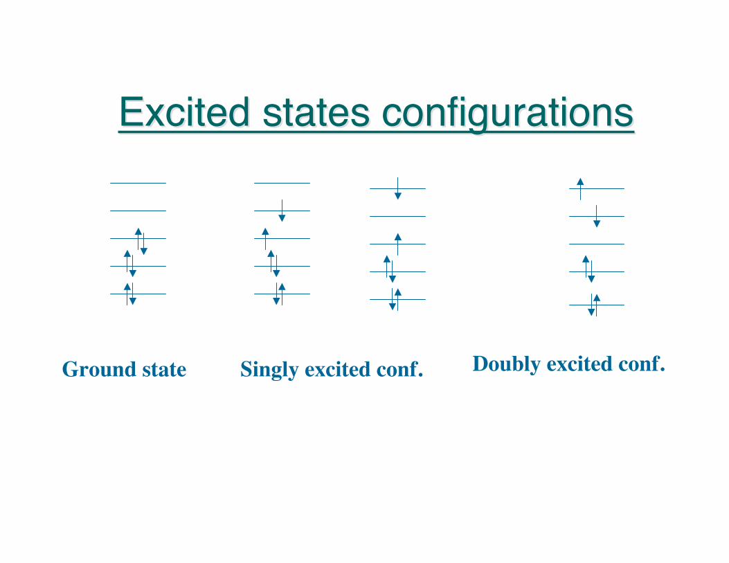
Excited states configurationsExcited states configurations

Singly excited conf. Doubly excited conf.Ground state

- +

Singlet CSF Triplet CSF

Configurations can be expressed as Slater determinants interms of molecular orbitals. Since in the nonrelativistic casethe eigenfunctions of the Hamiltoian are simultaneouseigenfunctions of the spin operator it is useful to useconfiguration state functions (CSFs)- spin adapted linearcombinations of Slater determinants, which areeigenfunctiosn of S2

Excited states can have very differentExcited states can have very differentcharacter and this makes their balancedcharacter and this makes their balanced

description even more difficult. For exampledescription even more difficult. For exampleexcited states can be:excited states can be:

• Valence states• Rydberg states• Charge transfer states

Rydberg Rydberg statesstates• Highly excited states where the electron is

excited to a diffuse hydrogen-like orbital• Low lying Rydberg states may be close to

valence states• Diffuse basis functions are needed for a proper

treatment of Rydberg states, otherwise thestates are shifted to much higher energies

• Diffuse orbitals need to be included in the activespace or in a restricted active space (RAS)

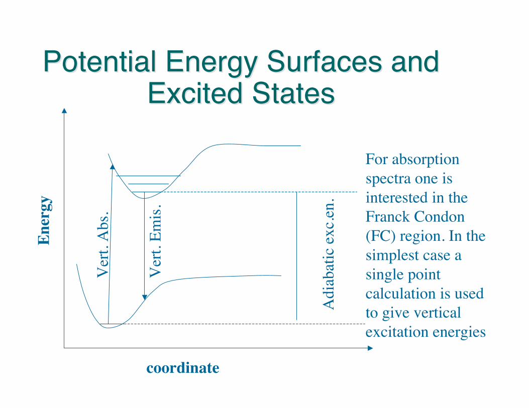
Potential Energy Surfaces andPotential Energy Surfaces andExcited StatesExcited States

Ver

t. A

bs.

Ver

t. Em

is .

Adi

abat

ic ex

c.en

.

Ener

gy

coordinate

For absorptionspectra one isinterested in theFranck Condon(FC) region. In thesimplest case asingle pointcalculation is usedto give verticalexcitation energies

When one is interested in the photochemistry andphotophysics of molecular systems the PES has to beexplored not only in the FC region but also alongdistorted geometries. Minima, transition states, andconical intersections need to be found (gradients forexcited states are needed)

Ener

gy

Reaction coordinate

TSTS

CICI

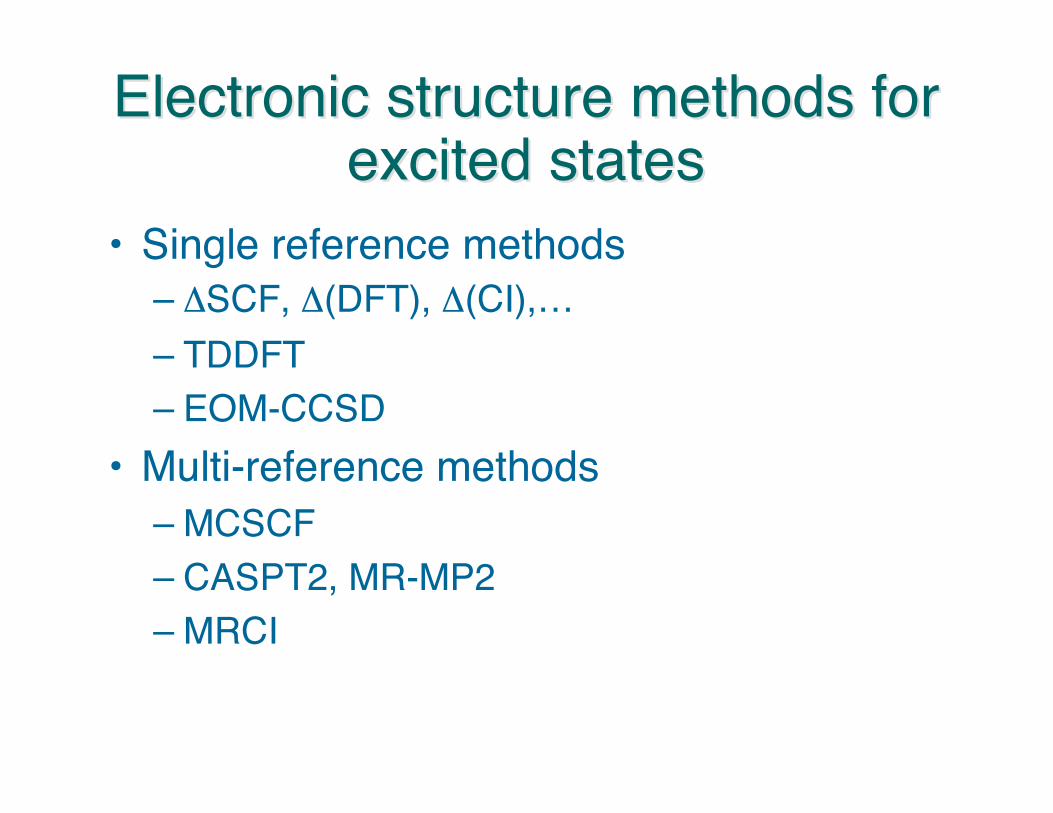
Electronic structure methods forElectronic structure methods forexcited statesexcited states

• Single reference methods– ΔSCF, Δ(DFT), Δ(CI),…– TDDFT– EOM-CCSD

• Multi-reference methods– MCSCF– CASPT2, MR-MP2– MRCI

• In the simplest case one can calculateexcited state energies as energydifferences of single-reference calculations.ΔE=E(e.s)-E(g.s.). This can be done:– For states of different symmetry– For states of different multiplicity– Possibly for states that occupy orbitals of

different symmetry

€

ΨCI = cmΨmm=1

NCSF

∑

Configuration InteractionConfiguration Interaction• Initially in any electronic structure calculation one

solves the HF equations and obtains MOs and aground state solution that does not include correlation

• The simplest way to include dynamical correlationand improve the HF solution is to use configurationinteraction. The wavefunction is constructed as alinear combination of many Slater determinants orconfiguration state functions (CSF). CI is a singlereference method but forms the basis for themultireference methods

Occupied orbitals

Virtual orbitals

Frozen orbitals

Frozen Virtual orbitals

Excitations fromoccupied tovirtual orbitals

Different orbital spaces in a CI calculationDifferent orbital spaces in a CI calculation

CSFs are created by distributing the electrons in the molecularorbitals obtained from the HF solution.

The variational principle is used for solving the Schrodingerequation

€

ΨCI = c0 HF + cirΨi

r

r

virt .

∑i

occ

∑ + cijrsΨij

rs

r<s

virt .

∑i< j

occ.

∑ + ...

€

ˆ H Ψ = EΨ

€

ˆ H = ˆ T e + ˆ V ee + ˆ V eN + ˆ V NN

=−1

2me

∇ i2

i∑ −

Zα

rαii∑

α

∑ +1rijj> i

∑i∑ +

ZαZβ

Rαββ >α

∑α

∑

= ˆ h ii∑ +

1rijj> i

∑i∑ + ˆ V NN

∫∫

ΨΨ

ΨΨ=

τ

τ

d

dE

*

*

var

H≥ 0

€

H11 − E H12 ... H1N

H21 H22 − E ... H2N

... ... ... ...H1N H2N ... HNN − E

= 0

Matrix formulation (NMatrix formulation (NCSFCSF x N x NCSFCSF))

For a linear trial function the variational principle leads to solving thesecular equation for the CI coefficients or diagonalizing the H matrix

The Hamiltonian can be computed and then diagonalized. Since thematrices are very big usually a direct diagonalization is used thatdoes not require storing the whole matrix.

€

Hmn = Ψm H Ψn

Number of singlet Number of singlet CSFsCSFsfor H2O with 6-31G(d)for H2O with 6-31G(d)

basisbasis

30046752102904475192449020181583655677147876621146665391126442596325562711

# CSFsExcitationlevel €

N =n!(n +1)!

m2

! m2

+1

! n − m

2

! n − m

2+1

!

•(m,n): distribute m electrons in n orbitals

Today expansions with billionof CSFs can be solved

0

0

00EHF

€

Ψir H Ψj

s

€

ΨHF H Ψijrs

€

ΨHF H Ψijrs

€

ΨHF H Ψir = 0

€

Ψkt H Ψij

rs€

Ψkt H Ψij

rs

dense

dense

dense

sparse

sparse€

Ψlmqp H Ψijk

rst

€

Ψlmqp H Ψijk

rst

sparse

sparse

CIS

ΨHF

ΨHF singles doubles triples

CISD

Brillouin’s thmCIS will give excited states but will leave the HF ground state unchanged

τφφφφφφ

τψψ

εετψψ

τψψ

τψψ

τψψ

dr

stpqwhere

bajiibjadH

iaiaEdH

theoremsBrillouindH

EdH

dHH

E

tstsqp

bj

ai

iaHFai

ai

ai

HF

jiij

iii

)]1()2()2()1([1)2()1()||(

),()||(

)||(

)'(0

12

0

00

−=

≠≠=

+−+=

=

=

=

=

∫

∫∫∫∫

∫

tHt

Condon-Slater rules are used toCondon-Slater rules are used toevaluate matrix elementsevaluate matrix elements

CISCIS• For singly excited states• HF quality of excited states• Overestimates the excitation energies• Can be combined with semiempirical methods

(ZINDO/S)

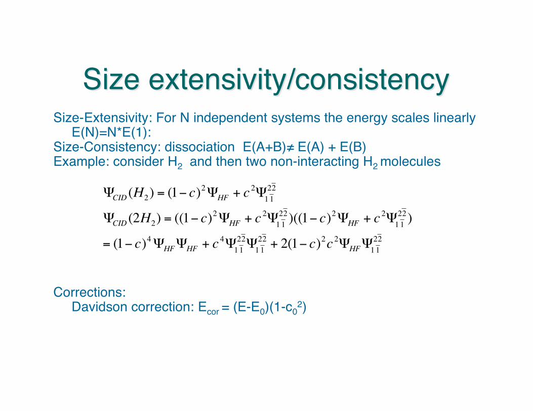
Size Size extensivityextensivity/consistency/consistencySize-Extensivity: For N independent systems the energy scales linearly

E(N)=N*E(1):Size-Consistency: dissociation E(A+B)≠ E(A) + E(B)Example: consider H2 and then two non-interacting H2 molecules

Corrections:Davidson correction: Ecor = (E-E0)(1-c0

2)€

ΨCID (H2) = (1− c)2ΨHF + c 2Ψ1 1 22

ΨCID (2H2) = ((1− c)2ΨHF + c 2Ψ1 1 22 )((1− c)2ΨHF + c 2Ψ1 1

22 )

= (1− c)4ΨHFΨHF + c 4Ψ1 1 22 Ψ1 1

22 + 2(1− c)2c 2ΨHFΨ1 1 22

Single reference Single reference vsvs..multireferencemultireference

• RHF for H2 : The Hartree-Fock wavefunction for H2 is

• The MO is a linear combinations of AOs: σ=1sA+ 1sB (spin is ignored)

• This wavefunction is correct at the minimum but dissociates into 50% H+H-

and 50% H·H·

€

Ψ =12σ (1)α(1) σ(1)β(1)σ (2)α(2) σ(2)β(2)

=

=12(σ (1)α(1)σ (2)β(2) −σ(1)β(1)σ(2)α(2)) =

=12(σ (1)σ (2))(α(1)β(2) −β(1)α(2))

€

Ψ =12(1sA (1) +1sB (1))(1sA (2) +1sB (2)) =

=12(1sA (1)1sB (2) +1sB (1)1sA (2) +1sA (1)1sA (2) +1sB (1)1sB (2))

Covalent H·H· Ionic H+H-

σg

σ u*

ionic H+H-

CI for HCI for H22• When two configurations are mixed:

• Ignore spin

• The coefficients c1 and c2 determine how the conf. Are mixed in order to getthe right character as the molecule dissociates. At the dissociation limit theorbitals σ, σ* are degenerate and c1=c2.

€

ΨCI = c1σ(1)α(1) σ (1)β(1)σ(2)α(2) σ (2)β(2)

+ c2σ * (1)α(1) σ * (1)β(1)σ * (2)α(2) σ * (2)β(2)

=

c1(σ(1)σ(2) + c2σ * (1)σ * (2))

€

Ψ = c1(1sA (1) +1sB (1))(1sA (2) +1sB (2))+c2(1sA (1) −1sB (1))(1sA (2) −1sB (2)) =

= c1(1sA (1)1sA (2) +1sB (1)1sB (2) +1sA (1)1sA (2) +1sB (1)1sB (2))+c2(1sA (1)1sA (2) +1sB (1)1sB (2) −1sA (1)1sA (2) −1sB (1)1sB (2))

Ionic H+H-

σg

σ u*

Ψ1 Ψ2

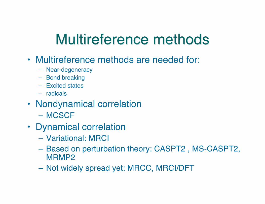
Multireference Multireference methodsmethods• Multireference methods are needed for:

– Near-degeneracy– Bond breaking– Excited states– radicals

• Nondynamical correlation– MCSCF

• Dynamical correlation– Variational: MRCI– Based on perturbation theory: CASPT2 , MS-CASPT2,

MRMP2– Not widely spread yet: MRCC, MRCI/DFT

Multiconfiguration Multiconfiguration Self-Self-Consistent Field TheoryConsistent Field Theory

(MCSCF)(MCSCF)• CSF: spin adapted linear combination of

Slater determinants

• Two optimizations have to be performed– Optimize the MO coefficients– optimize the expansion coefficients of the CSFs

€

ΨMCSCF = cn CSFn=1

CSFs

∑

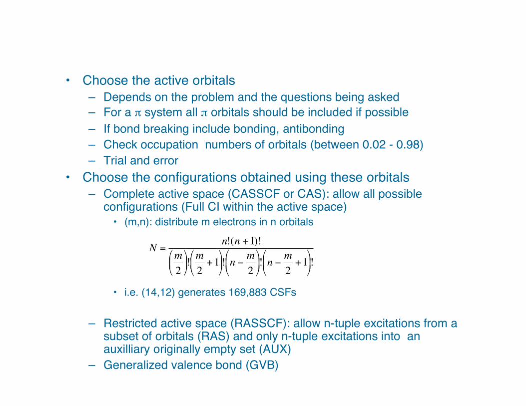
• Choose the active orbitals– Depends on the problem and the questions being asked– For a π system all π orbitals should be included if possible– If bond breaking include bonding, antibonding– Check occupation numbers of orbitals (between 0.02 - 0.98)– Trial and error

• Choose the configurations obtained using these orbitals– Complete active space (CASSCF or CAS): allow all possible

configurations (Full CI within the active space)• (m,n): distribute m electrons in n orbitals

• i.e. (14,12) generates 169,883 CSFs

– Restricted active space (RASSCF): allow n-tuple excitations from asubset of orbitals (RAS) and only n-tuple excitations into anauxilliary originally empty set (AUX)

– Generalized valence bond (GVB)

€

N =n!(n +1)!

m2

! m2

+1

! n − m

2

! n − m

2+1

!

CAS

Virtual orbitals

Double occupied orbitals

CAS

Virtual orbitals

DOCC orbitals

RAS: n excitationsout permitted

AUX:nexcitationsin permitted

CASSCF RASSCF

Orbital spaces in an MCSCF calculationsOrbital spaces in an MCSCF calculations

• The choice of the active space determines the accuracy of themethod. It requires some knowledge of the system and carefultesting.

• For small systems all valence orbitals can be included in the activespace

• For conjugated systems all π orbitals if possible should be includedin the active space. For heteroatomic rings the lone pairs should beincluded also. What cas should be chosen for the followingsystems?– N2– Ozone– Allyl radical– Benzene– Uracil

The most important question inThe most important question inmultireference multireference methods:methods:

Choosing the active spaceChoosing the active space

State averaged MCSCFState averaged MCSCF• All states of interest must be included in the average• When the potential energy surface is calculated, all states

of interest across the coordinate space must be includedin the average

• State-averaged MOs describe a particular state poorerthan state-specific MOs optimized for that state

• State-average is needed in order to calculate all stateswith similar accuracy using a common set of orbitals. Thisis the only choice for near degenerate states, avoidedcrossings, conical intersections.

• Provides common set of orbitals for transition dipoles andoscillator strengths

Multireference Multireference configurationconfigurationinteractioninteraction

• Includes dynamical correlation beyond theMCSCF

• Orbitals from an MCSCF (state-averaged) areused for the subsequent MRCI

• The states must be described qualitativelycorrect at the MCSCF level. For example, if 4states are of interest but the 4th state at theMRCI level is the 5th state at the MCSCF level a5-state average MCSCF is needed

CAS

Virtual orbitals

DOCC orbitals

Frozen orbitals

MRCIMRCIFrozen Virtualorbitals

•A reference space is neededsimilar to the active space atMCSCF

•References are created withinthat space

•Single and double excitationsusing each one of thesereferences as a starting point

•ΨMRCI=∑ciΨi

CASPT2CASPT2• Second order perturbation theory is used

to include dynamic correlation• Has been used widely for medium size

conjugated organic systems• Errors for excitation energies ~0.3 eV• There are no analytic gradients available

so it is difficult to be used for geometryoptimizations and dynamics

COLUMBUSCOLUMBUS• Ab initio package• MCSCF• MRCI• Analytic gradients for MRCI• Graphical Unitary Group Approach

(GUGA)

Colinp Colinp (input script)(input script)• Integral• SCF• MCSCF• CI• Control input