Embed Size (px)
DESCRIPTION
Electromagnetic testing emt-acfm chapter 10c - revised
Citation preview
Charlie Chong/ Fion Zhang
Electromagnetic TestingMFLT/ ECT/ Microwave/RFTChapter 10C – ACFMAlternating Current Field Measurement 14th Feb 2015My ASNT Level III Pre-Exam Preparatory Self Study Notes

Charlie Chong/ Fion Zhang
ACFM - The alternative NDT Method
Charlie Chong/ Fion Zhang
ACFM - The alternative NDT Method
Charlie Chong/ Fion Zhang
ACFM - The alternative NDT Method

Charlie Chong/ Fion Zhang

Charlie Chong/ Fion Zhang
NDT Level III ExaminationsBasic and Method ExamsASNT NDT Level III certification candidates are required to pass both the NDT Basic and a method examination in order to receive the ASNT NDT Level III certificate.Exam SpecificationsThe table below lists the number of questions and time allowed for each exam. Clicking on an exam will take you to an abbreviated topical outline and reference page for that exam. For the full topical outlines and complete list of references, see the topical outlines listed in the American National Standard ANSI/ASNT CP-105, Standard Topical Outlines for Qualification of Nondestructive Testing Personnel.
ETElectromagnetic Testing135 Questions 4 hrs Papers Certification: NDT only

Fion Zhang at Shanghai2015 February
苏州太湖 2014

Charlie Chong/ Fion Zhang
Charlie Chong/ Fion Zhang
Alternating Current Field Measurement ACFM - Reading Session Three
Charlie Chong/ Fion Zhang
Reading 1: Sizing and tomography of rolling contact fatigue cracks in rails using NDT technology – potential for high speed applicationAbstractRolling contact fatigue (RCF) cracks in the rail head progressively grow due to in-service loading. Early detection and sizing of RCF cracks allows more efficient mediation treatment such as grinding. In this paper the capability of an Alternating Current Field Measurement (ACFM) technique to detect and size light to moderate RCF cracks, both at high speed (up to 120 km/h) is discussed. Experimental and computer modelling results have shown that crack detection with improved characterisation information can be achieved using a single ACFM probe. Further work is now in progress that brings together a multi-probe sensor with high speed electronic processing to provide a practical system suitable for attachment to a specialist measurement train.
Keywords Non-destructive testing; Alternating Current Field Measurement; Rolling Contact Fatigue.
http://www.shipstructure.org/pdf/91symp22.pdf
Charlie Chong/ Fion Zhang
Introduction
An increase in capacity (higher travel speeds and axle loads) on modern railways increases the dynamic loading on the rails and hence track degradation. To maintain high operational safety at minimal cost, condition monitoring of rail tracks requires methods for early detection of rolling contact fatigue (RCF) cracks and their growth in service. Currently ultrasonic inspection is carried out by a variety of different instruments ranging from hand-held devices, through to dual-purpose road/track vehicles to test fixtures that are towed or carried by dedicated rail cars. Unfortunately, the performance of existing conventional ultrasonic probes in detecting small (<4 mm depth) surface defects such as head checks and gauge corner cracking is inadequate during high speed inspection. In addition, the presence of larger and more critical internal defects can be shadowed by smaller surface cracks during inspection. This is also one of the reasons that the current international practice is to combine non-destructive evaluation of the rail network with reventative maintenance procedures, such as rail head grinding, in order tooptimise the trade-off between maintenance cost and structural reliability
Charlie Chong/ Fion Zhang
Inspection systems based on the simultaneous use of conventional ultrasonic transducers with magnetic flux leakage (MFL) sensors have a higher probability of detecting smaller near-surface and surface-breaking defects in the rail head. However, as inspection speed increases, the performance of MFL sensors tends to deteriorate rapidly due to a reduction in the magnetic flux density. More recently, pulsed eddy current (PEC) probes have been added on certain ultrasonic test trains to offer increased sensitivity in the detection of surface defects at high inspection speed. PEC probes perform far better than MFL sensors at higher inspection speeds but are affected more by lift-off variation and typically need to be position at <2mm from the rail head.
Alternating current field measurement (ACFM) sensors are less sensitive to lift off (up to at 5 mm lift off from the rail head) than the PEC probes, have the potential to operate at high speeds and provide information that can be used to size and shape RCF cracks, the system can be used in the form of a walking stick on the UK network. This paper summarises some of the recent advances in using the ACFM technique for rail NDT.

Charlie Chong/ Fion Zhang
Proof of principle: ACFM operation at high speed
ACFM experiments were carried out at inspection speeds up to 121.5 kmh-1
using a turning lathe-based test rig. A high-speed single channel micro pencil probe manufactured by TSC Inspection Systems Ltd. Was utilised during testing. The pencil probe operated at a frequency of 50 kHz and was driven by a commercial TSC AMIGO instrument. The data obtained were logged using customised software on a PC that incorporated a high-speed data acquisition board. The data acquisition rate during tests was 1 MHz. To test the overall capability and performance of the ACFM system at high inspection speeds under controlled experimental conditions a special rotary test piece was manufactured.
Charlie Chong/ Fion Zhang
The material used for manufacturing the rotary test piece was a 0.9 wt % C steel to make sure that the microstructure, as well as the relative magnetic permeability and electrical conductivity are similar to those exhibited by conventional 260 rail steel grade (typically 0.7-0.8 wt % C), with both steels having a predominantly pearlitic microstructure. The rotary test piece had a 230 mm diameter and was 60 mm thick with a bore in the centre 190 mm in diameter and 50 mm deep. Four transverse notches (2 x 2 mm and 2 x 4 mm deep with a flat profile) were spark eroded at the centre of the 20 mm wide rim of the sample. Each notch was 10 mm long and 0.5 mm wide. The sample was placed in a turning lathe capable of rotating the test piece between 1 to 3000 revolutions per minute (rpm). The rotational speed of 1 rpm for this experimental setup corresponded to the equivalent of a surface speed of 0.0405 kmh-1 at the centre of the notch (i.e. 10 mm away from the edge of the rim) and hence at 3000 rpm the surface speed of the sample at the centre of the notches was 121.5 kmh-1.
Charlie Chong/ Fion Zhang
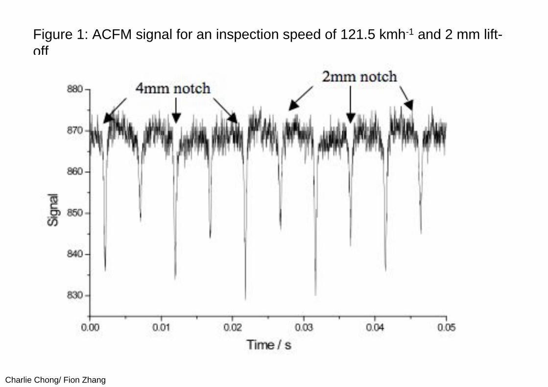
The ACFM probe was positioned opposite to the centre of the notches and at a 0° angle with reference to their surface orientation. Figure 1 shows the ACFM signal obtained for a probe lift-off of 2mm at an inspection speed of 121.5kmh-1.
Charlie Chong/ Fion Zhang
Figure 1: ACFM signal for an inspection speed of 121.5 kmh-1 and 2 mm lift-off
Charlie Chong/ Fion Zhang
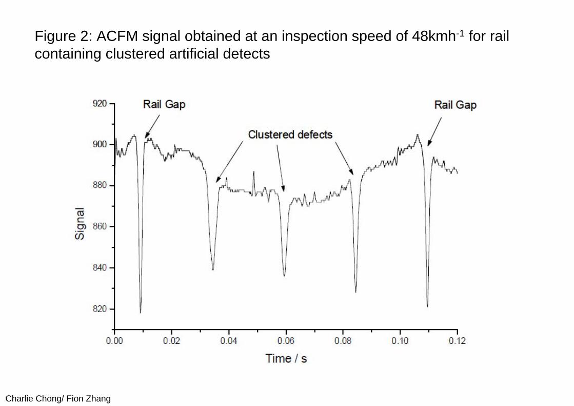
To extend the analysis to consider inspection of rails a 3.6 m diameter spinning rail rig, capable of rotating at speeds between 1 to 80 kmh-1, with a special set of eight 1.41 m long rails containing artificially induced defects (including half-face slots machined normal to the railhead surface, clusters of angled slots, and pocket defects more typical of real defects) was used. The ACFM probe was installed on a customised trolley placed on the rails while the rig was rotated at 1.6 kmh-1, progressively increasing its speed up to 48 kmh-1. Figure 2 shows the ACFM signal obtained at 48 kmh-1 showing that the artificial defect clusters can be successfully detected, further results are published elsewhere
Charlie Chong/ Fion Zhang
Figure 2: ACFM signal obtained at an inspection speed of 48kmh-1 for rail containing clustered artificial detects
Charlie Chong/ Fion Zhang
Modelling of light-moderate RCF cracks for size and shape analysis:
A finite element method (FEM) model, using COMSOL Multiphysics software, has been developed to model the ACFM sensor response to both ideal and real defects in rail. The commercial AMIGO software currently sizes crack using estimations based on the theory for regularly sized cracks, in addition the walking stick ACFM system has had empirical corrections added in, based on experimental data from destructive tests of RCF cracks (for cracks with pocket length > 4 mm). The COMSOL model allows non-regular cracks with a wider variation of pocket length and shapes, as well as overlapping cracks to be accurately assessed. In addition, comparisons between elliptical approximations and actual RCF crack shapes (for light-moderate RCF cracks) have been carried out.
Charlie Chong/ Fion Zhang
The defects are modelled in three dimensions, with a very fine mesh concentrated around the regions of interest, namely the defect and a layer above the surface of the rail where measurements are taken. Modelling was carried out using an impedance boundary condition between the rail surface and the surrounding air. This implies that the current travels along the boundary, greatly simplifying the model and allowing solutions to be found for complex crack shapes. The error of this assumption is negligible due to the very small skin depth in steel at the high probe operation equency. Additional detail on the modelling approach are presented elsewhere
Charlie Chong/ Fion Zhang
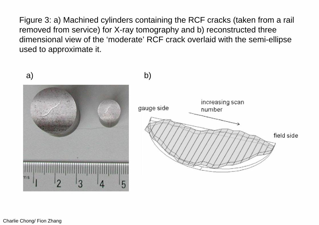
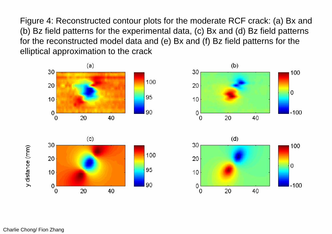
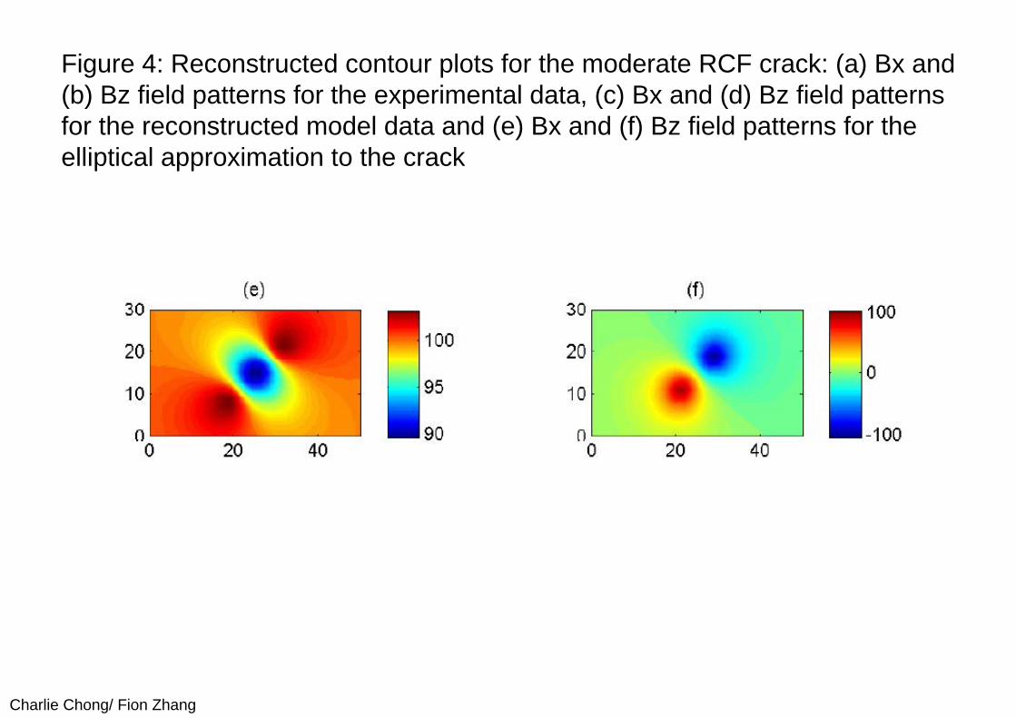
Two RCF cracks, a ‘light’ crack (according to the Railtrack classification system [19] with a surface length of 4.93 mm) and a ‘moderate’ crack (surface length of 12.92 mm) that had developed in a section of rail taken from service, have been assessed. Figure 3 shows images of the two real RCF cracks and a virtual reconstruction of the moderate crack from X-ray tomography images. The vertical angle of propagation was found to be 34° for the light crack and 25° for the moderate one. Contour plots have been reconstructed from the experimental and model scans and are shown in Figure 4 for the moderate crack. Plots (a) and (b) show the experimental results, plots (c) and (d) the reconstructed crack model data and (e) and (f) the results from an elliptical approximation to the crack shape. It can be seen from Figure 4 that there is very good qualitative agreement between the experimental results and the model results, both for the actual crack shape and elliptical approximation, a similar level of agreement was seen for the light RCF crack.
Charlie Chong/ Fion Zhang
Figure 3: a) Machined cylinders containing the RCF cracks (taken from a rail removed from service) for X-ray tomography and b) reconstructed three dimensional view of the ‘moderate’ RCF crack overlaid with the semi-ellipse used to approximate it.
a) b)
Charlie Chong/ Fion Zhang
Figure 4: Reconstructed contour plots for the moderate RCF crack: (a) Bx and (b) Bz field patterns for the experimental data, (c) Bx and (d) Bz field patterns for the reconstructed model data and (e) Bx and (f) Bz field patterns for the elliptical approximation to the crack
Charlie Chong/ Fion Zhang
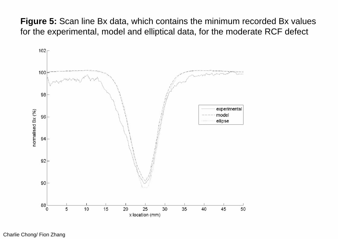
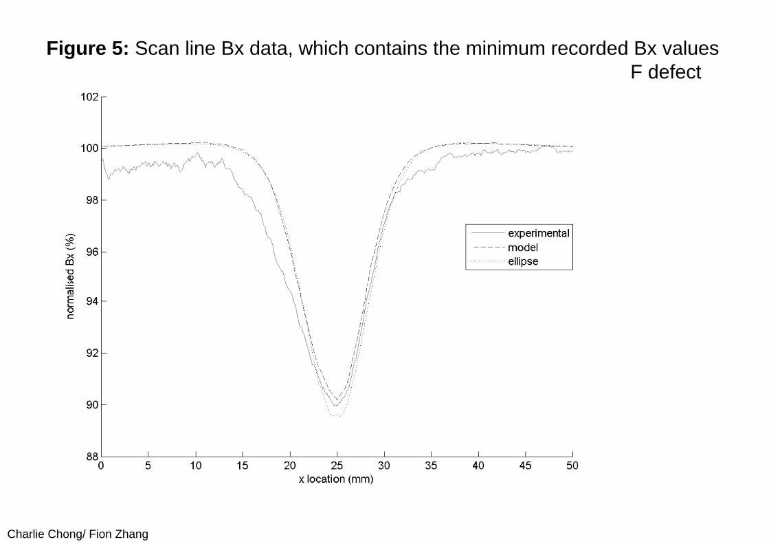
Figure 5 shows the Bx data for the scan line across the moderate RCF crack that achieved the minimum normalised Bx values (this approach represents using an array of sensors (for a high speed approach) or a single probe sensor and, for example, a robot arm to conduct multiple scans for tomographic information.
Overall it can be seen that the predicted ACFM signal changes from a COMSOL model using a semi-elliptical crack to represent the moderate RCF crack in a rail removed from service provides good agreement to the measured ACFM signals. It should be noted that the effective rail maintenance planning requires the vertical depth to which the cracks reach, if grinding regimes are to be optimised to remove the RCF defects. In order to predict this from the ACFM data the model requires the crack angle of propagation into the surface of the rail (typically 20-35° before the cracks turn down at approximately 5 mm vertical depth). The effect of variations in crack shape, orientation and size, including for larger RCF cracks, which are known to be non-elliptical in shape, on the ACFM signal is being researched at present.
Charlie Chong/ Fion Zhang
Figure 5: Scan line Bx data, which contains the minimum recorded Bx values for the experimental, model and elliptical data, for the moderate RCF defect
Charlie Chong/ Fion Zhang
Figure 5: Scan line Bx data, which contains the minimum recorded Bx values for the experimental, model and elliptical data, for the moderate RCF defect
Charlie Chong/ Fion Zhang
Optimisation of ACFM inspection on rail
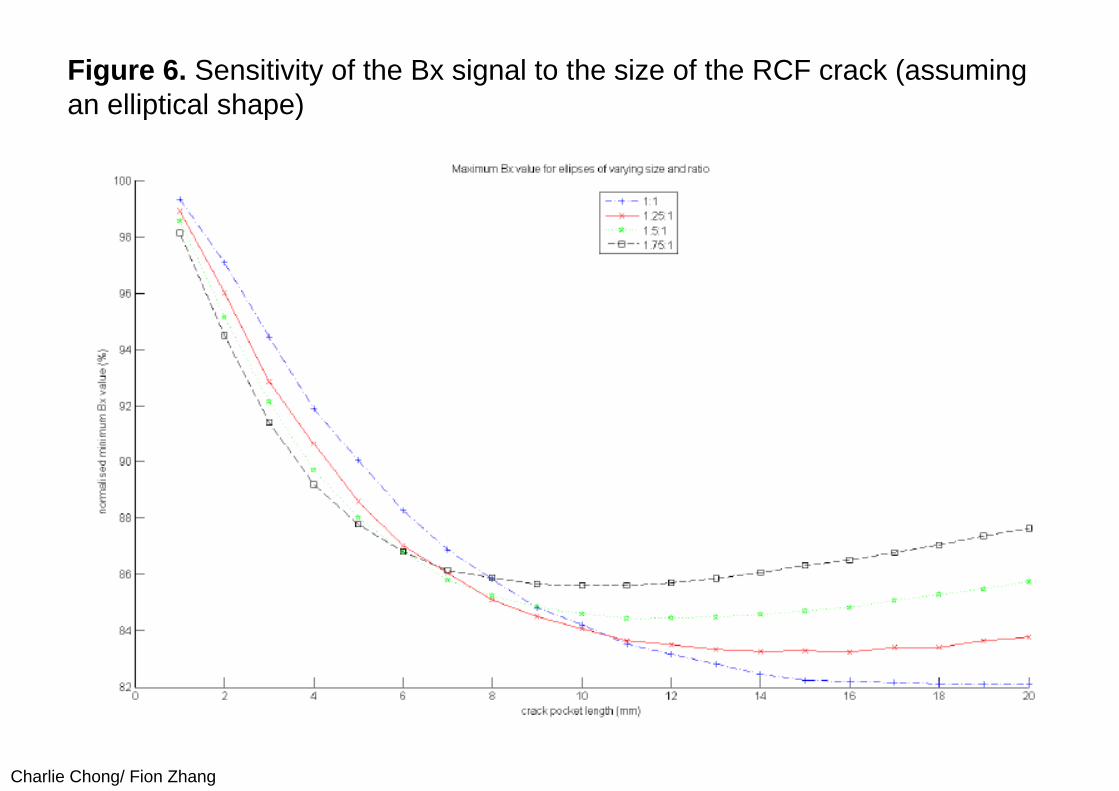
RCF cracks on rails form at varying angles to the rail length, frequently between 30° and 45°, and at varying propagation angles (typically 20-35°) . The ACFM sensor signal is sensitive to the size, shape and orientation of the RCF cracks. In order to determine whether accurate sizing of cracks can be achieved in principle the sensitivity of the signal to these factors needs to be determined. Figure 6 shows the effect on the Bx signal of changing the size of modelled semi-elliptical cracks. Semiellipses of surface length 1 to 20 mm for four elliptical ratios, a:b, for a = 1, 1.25, 1.5 and 1.75 and b = 1, where a is the semi-major axis and b is the semi-minor axis, have been modelled. The model is based on a 5 kHz ACFM sensor. In Figure 6 the minimum Bx value for each semi-ellipse is plotted against the crack pocket length. This value, along with the distance between the Bz trough and peak and the background Bx value may be used to give an accurate estimate of the crack pocket length. This is achieved in the AMIGO software using a lookup table based on analytical theory. However, above a certain crack pocket length, sensitivity of the Bx signal to increasing pocket length saturates.
Charlie Chong/ Fion Zhang
From Figure 6 it can be seen that the minimum Bx value initially decreases steeply as crack pocket length increases. For cracks with a pocket length in this region, the ACFM Bx signal can effectively be used to size the crack. However, as pocket length increases further, the sensitivity of the ACFM Bx signal to increasing pocket length begins to saturate; for the semi-ellipses modelled here, this occurs at between 10 mm pocket length (for the 1.75:1 ratio semi-ellipse) and 19 mm (for the 1:1 semi-ellipse), corresponding to crack surface lengths of 35 to 38 mm.
Charlie Chong/ Fion Zhang
Figure 6. Sensitivity of the Bx signal to the size of the RCF crack (assuming an elliptical shape)
Charlie Chong/ Fion Zhang
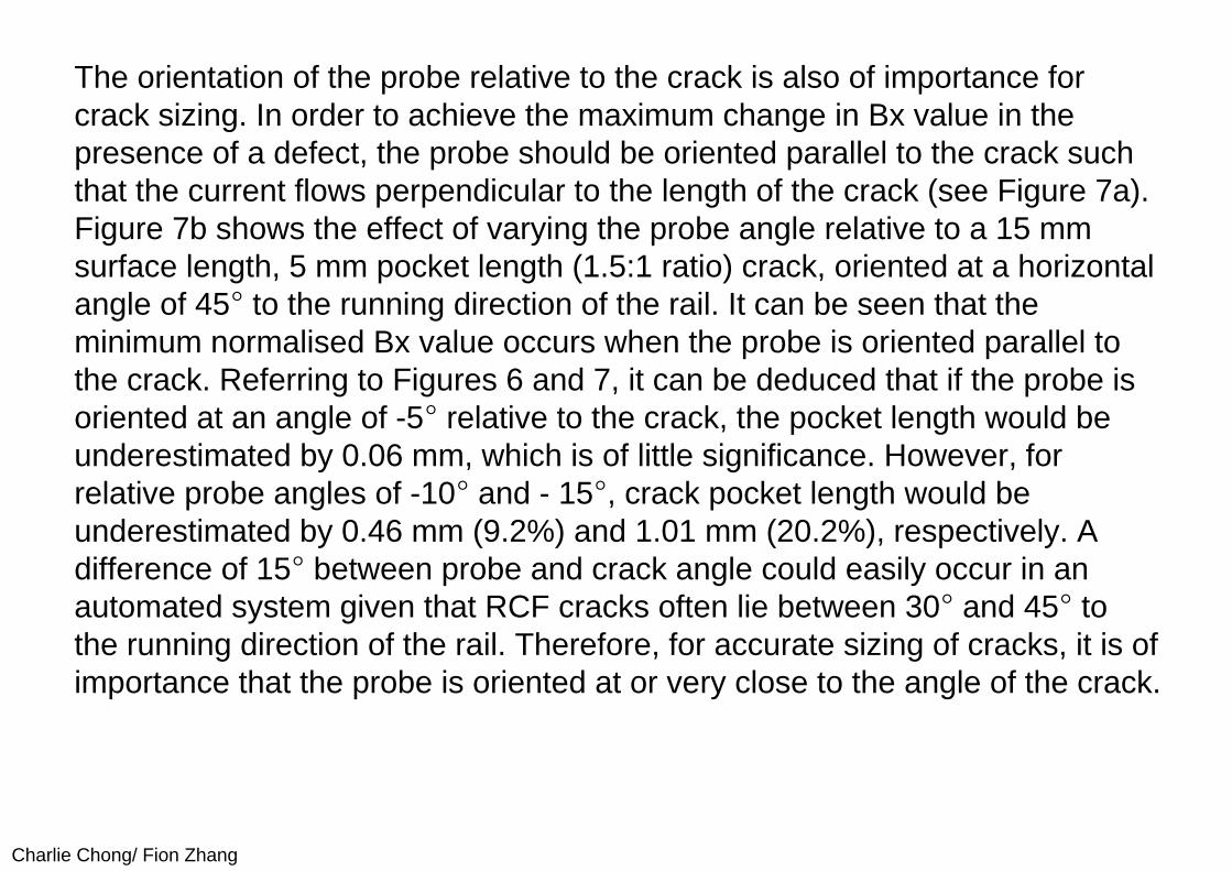
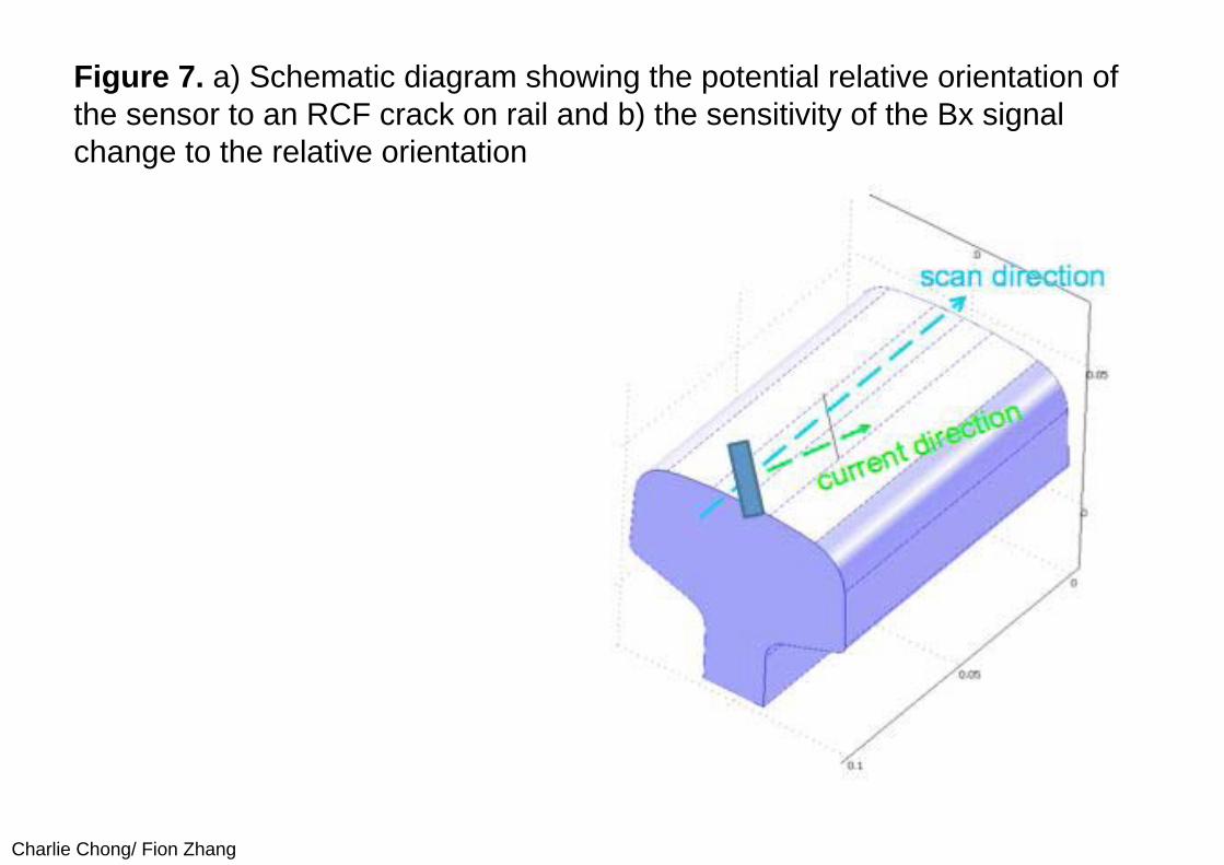
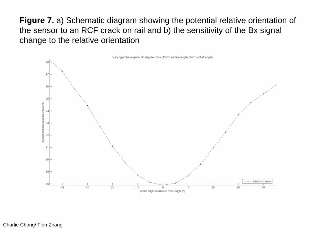
The orientation of the probe relative to the crack is also of importance for crack sizing. In order to achieve the maximum change in Bx value in the presence of a defect, the probe should be oriented parallel to the crack such that the current flows perpendicular to the length of the crack (see Figure 7a). Figure 7b shows the effect of varying the probe angle relative to a 15 mm surface length, 5 mm pocket length (1.5:1 ratio) crack, oriented at a horizontal angle of 45° to the running direction of the rail. It can be seen that the minimum normalised Bx value occurs when the probe is oriented parallel to the crack. Referring to Figures 6 and 7, it can be deduced that if the probe is oriented at an angle of -5° relative to the crack, the pocket length would be underestimated by 0.06 mm, which is of little significance. However, for relative probe angles of -10° and - 15°, crack pocket length would be underestimated by 0.46 mm (9.2%) and 1.01 mm (20.2%), respectively. A difference of 15° between probe and crack angle could easily occur in an automated system given that RCF cracks often lie between 30° and 45° to the running direction of the rail. Therefore, for accurate sizing of cracks, it is of importance that the probe is oriented at or very close to the angle of the crack.
Charlie Chong/ Fion Zhang
Note also that knowledge of the vertical angle of propagation of the crack is necessary to determine crack depth for implementation of a grinding regime. The ACFM signal does not give information about crack propagation angle, or equivalently crack depth.
Charlie Chong/ Fion Zhang
Figure 7. a) Schematic diagram showing the potential relative orientation of the sensor to an RCF crack on rail and b) the sensitivity of the Bx signal change to the relative orientation
Charlie Chong/ Fion Zhang
Figure 7. a) Schematic diagram showing the potential relative orientation of the sensor to an RCF crack on rail and b) the sensitivity of the Bx signal change to the relative orientation
Charlie Chong/ Fion Zhang
Implementation and future work
Experimental and computer modelling results have shown that crack detection with improved characterisation information can be achieved using a single ACFM probe. Work is now underway to develop a specialist rail test sensor that incorporates eight individual pencil probes. This sensor will be used on a test train. Using such a sensor it will be possible to inspect the whole rail head with a single passage. In order to be able to process the data from the eight probes in parallel, and at a speed that would allow a sensor to be fitted to a practical measurement train (i.e. up to 120 kmh-1), it is necessary to utilise advanced high speed electronics. The existing pencil probe processing is based around analogue electronics. In order to address the requirement of high speed, parallel processing a new digital, data acquisition and processing architecture has been developed based that uses field programmable gate array (FPGA) technology. FPGAs are integrated circuits that contain programmable logic blocks and reconfigurable interconnections. Complex functions can be programmed using hardware description language (HDL). The results of this work will be demonstrated as part of the European Commission FP7 Project INTERAIL.
Charlie Chong/ Fion Zhang
Reading 2: The First 20 years of the A.C. field Measurement Technique
Abstract: The A.C. Field Measurement technique was originally developed as a non-contacting version of the A.C. Potential Drop technique, with the aim of accurately measuring the depth of surface-breaking fatigue cracks at welds underwater. Since then, the technique has expanded into many diverse applications, both underwater and in air. This paper describes the evolution of ACFM equipment from the first commercial systems produced in 1991 for underwater inspection of welded offshore structures, to the current sophisticated, semi-automated array systems. Examples are given for inspection of threaded connections in the mining industry, robotic inspection of coke drum linings, and latest developments for train-mounted high speed rail inspection.
Keywords: A.C. field measurement (ACFM), rail, wheelsets, threads, coke-drum, robotic deployment
http://www.tscinspectionsystems.co.uk/pdfdocs/ApplicationCrackGrowthMonitoring.pdf
Charlie Chong/ Fion Zhang
1. Introduction
In the mid 1980’s, oil companies working in the North Sea were looking for a technique better suited to estimating the depths of fatigue cracks found underwater at welded intersections by magnetic particle inspection (MPI). A.C. potential drop (ACPD) was one technique being used for this purpose at the time, but it was very difficult and slow to use underwater because of the need to maintain very good electrical contact between the voltage probe and the surface.
A non-contacting equivalent to ACPD was required. The mechanical engineering department at University College London (UCL) had many years experience in both theoretical and practical developments in ACPD, so a group of UK oil companies approached them to develop the new technique, which became known as a.c. field measurement (ACFM).
Charlie Chong/ Fion Zhang
Principle of ACFM
ACFM uses induced rather than injected currents but maintains, as far as possible, the same uniform strength, unidirectional currents as ACPD. This is the main differentiating factor from conventional eddy current techniques. This allowed UCL to take existing theoretical models of the effect of semi-elliptical surface breaking defects on the current flow and to extend them to predict the effect on the associated magnetic fields above the surface. By measuring components of these magnetic fields and comparing the results with the theoretical predictions, ACFM is able to determine the length and depth of a defect without having to calibrate on slots.
The theoretical model, and early experimental results, were published in 1988 and in 1991, the first commercial instruments were made. Over the following 20 years, ACFM has expanded worldwide into a useful addition to the NDT toolbox, particularly for inspecting painted or coated, welded steel structures.
Charlie Chong/ Fion Zhang
Keywords:
Induced current, uniform field, unidirectional current. Semi-elliptical surface breaking theoretical models, Semi-elliptical surface breaking defects on the current flow and to extend
them to predict the effect on the associated magnetic fields above the surface.
By measuring components of these magnetic fields and comparing the results with the theoretical predictions, ACFM is able to determine the length and depth of a defect without having to calibrate on slots.
Discuss on: unidirectional current induced.
Charlie Chong/ Fion Zhang
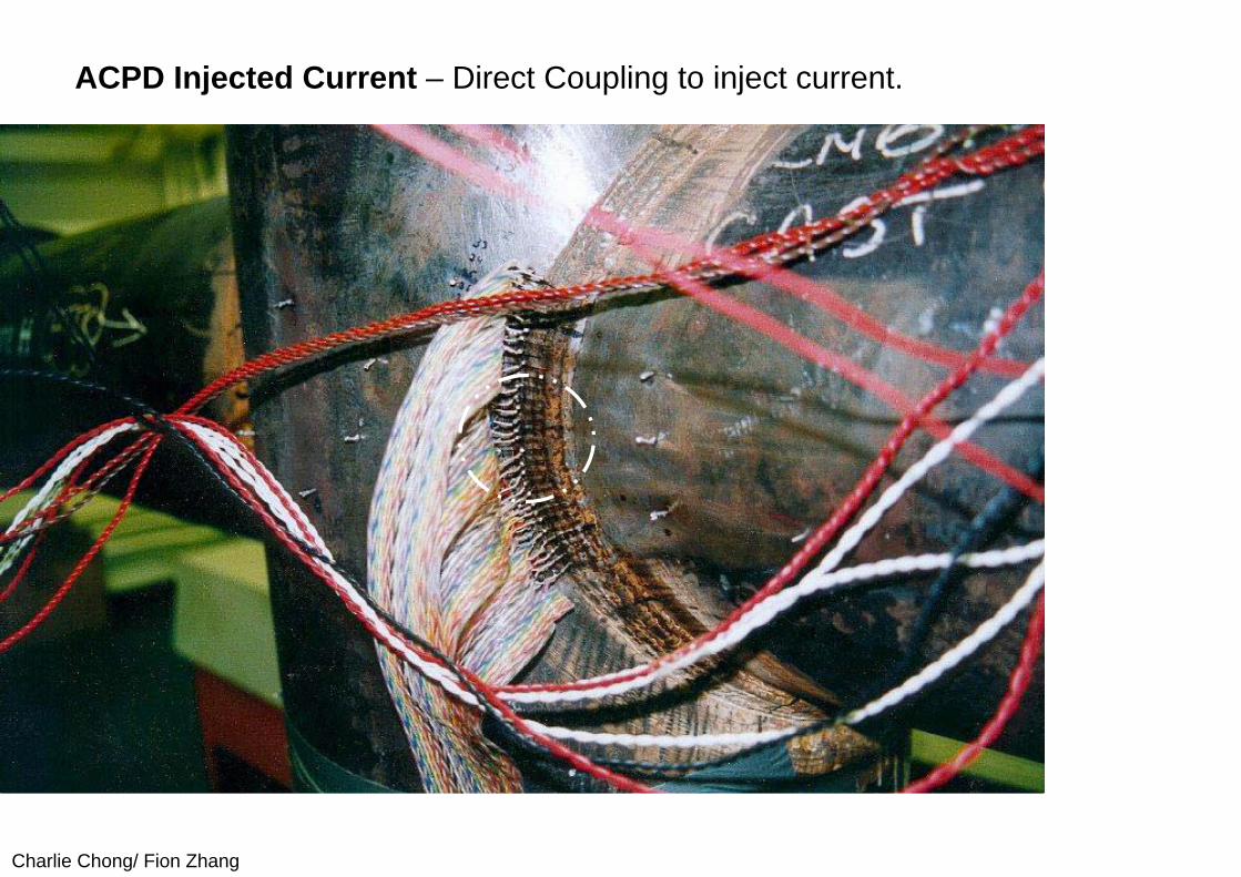
ACPD Injected Current – Direct Coupling to inject current.
Charlie Chong/ Fion Zhang
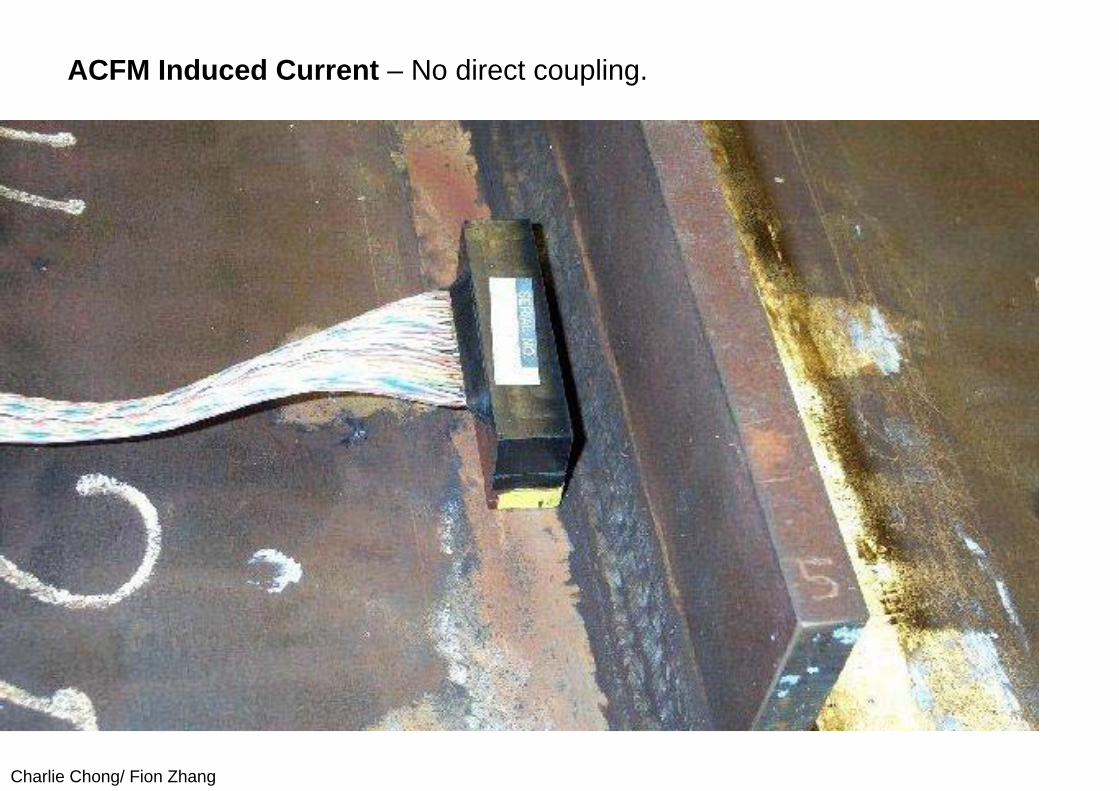
ACFM Induced Current – No direct coupling.
Charlie Chong/ Fion Zhang
2. The ACFM Technique.
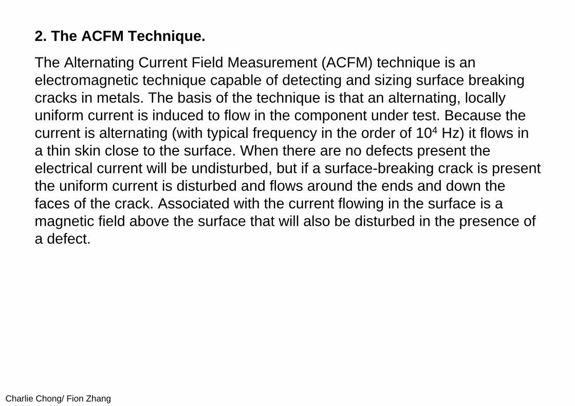
The Alternating Current Field Measurement (ACFM) technique is anelectromagnetic technique capable of detecting and sizing surface breaking cracks in metals. The basis of the technique is that an alternating, locally uniform current is induced to flow in the component under test. Because the current is alternating (with typical frequency in the order of 104 Hz) it flows in a thin skin close to the surface. When there are no defects present the electrical current will be undisturbed, but if a surface-breaking crack is present the uniform current is disturbed and flows around the ends and down the faces of the crack. Associated with the current flowing in the surface is a magnetic field above the surface that will also be disturbed in the presence of a defect.
Charlie Chong/ Fion Zhang
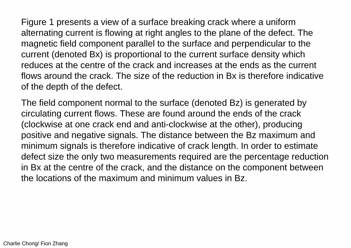
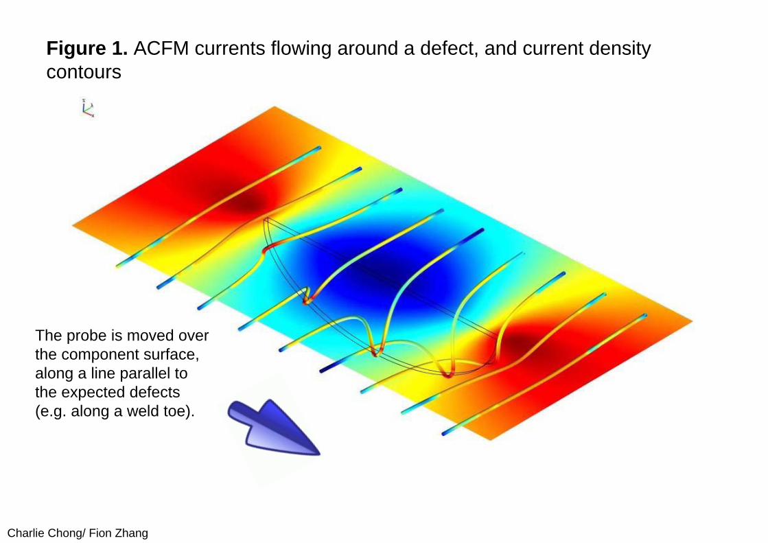
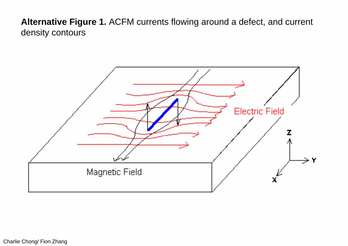
Figure 1 presents a view of a surface breaking crack where a uniform alternating current is flowing at right angles to the plane of the defect. The magnetic field component parallel to the surface and perpendicular to the current (denoted Bx) is proportional to the current surface density which reduces at the centre of the crack and increases at the ends as the current flows around the crack. The size of the reduction in Bx is therefore indicative of the depth of the defect.
The field component normal to the surface (denoted Bz) is generated by circulating current flows. These are found around the ends of the crack (clockwise at one crack end and anti-clockwise at the other), producing positive and negative signals. The distance between the Bz maximum and minimum signals is therefore indicative of crack length. In order to estimate defect size the only two measurements required are the percentage reduction in Bx at the centre of the crack, and the distance on the component between the locations of the maximum and minimum values in Bz.
Charlie Chong/ Fion Zhang
Figure 1. ACFM currents flowing around a defect, and current density contours
The probe is moved over the component surface, along a line parallel to the expected defects (e.g. along a weld toe).
Charlie Chong/ Fion Zhang
Alternative Figure 1. ACFM currents flowing around a defect, and current density contours
Charlie Chong/ Fion Zhang
From a practical standpoint, standard ACFM probes contain a remote field induction system, usually a horizontal solenoid or yoke above the surface, together with two orthogonal magnetic field sensors close to the surface that allow measurement of the two components of magnetic field at the same point in space.
The probe requires no electrical or mechanical contact with the component and can therefore be applied without the removal of surface coatings or grime. In order to collect the required data, the probe is moved over the component surface, along a line parallel to the expected defects (e.g. along a weld toe).
The use of a uniform input field provides other benefits, in addition to the ability to model the field-defect interactions. For example, signals vary relatively slowly with probe stand-off from the surface, so surface roughness or large coating thicknesses cause less of a problem than for conventional eddy current inspection. Also, by scanning parallel to the defect, rather than across it, ACFM has less of a problem inspecting at interfaces between different materials.
Charlie Chong/ Fion Zhang
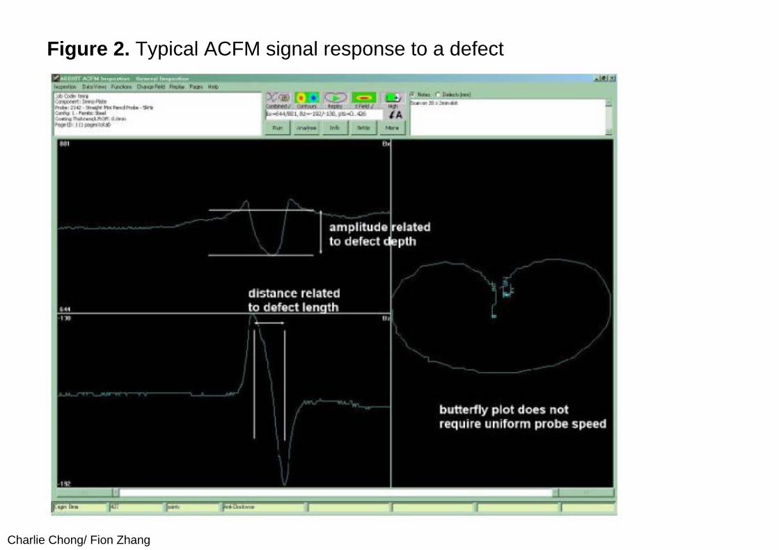
A standard PC is used to control the equipment and display results. The plot on the left of Figure 2 shows typical raw data from the crack end (Bz) and crack depth (Bx) sensors collected from a manually deployed probe. The right hand section of Figure 2 shows the same data presented as a so-called butterfly plot, in which Bx is plotted against Bz. In the presence of a defect, a loop reminiscent of a butterfly is drawn in the screen and the operator looks for this distinctive shape to decide whether a crack is present or not. All data is stored by the system and is available for subsequent review and analysis. This is particularly useful for audit purposes and for reporting.
Charlie Chong/ Fion Zhang
Figure 2. Typical ACFM signal response to a defect
Charlie Chong/ Fion Zhang
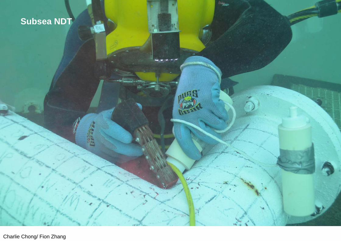
Since the ACFM technique was originally developed for sizing cracks underwater, the first practical system was an underwater one. The first subsea instrument to utilise the ACFM technique (the U11) was built in 1991.
Although developed for sizing defects found by other techniques (usually magnetic particle inspection), the fact that ACFM probes work through rust and paint etc. mean that ACFM is also well suited as a detection technique. The prototype was used in a series of Probability of Detection trials on real fatigue cracks on tubular welded intersections in a diving tank at City University, London. The results demonstrated that ACFM was at least as good as MPI for detection, and with the added advantage of providing defect depth information accurate to about +/- 15%.
Charlie Chong/ Fion Zhang
Subsea NDT
Charlie Chong/ Fion Zhang
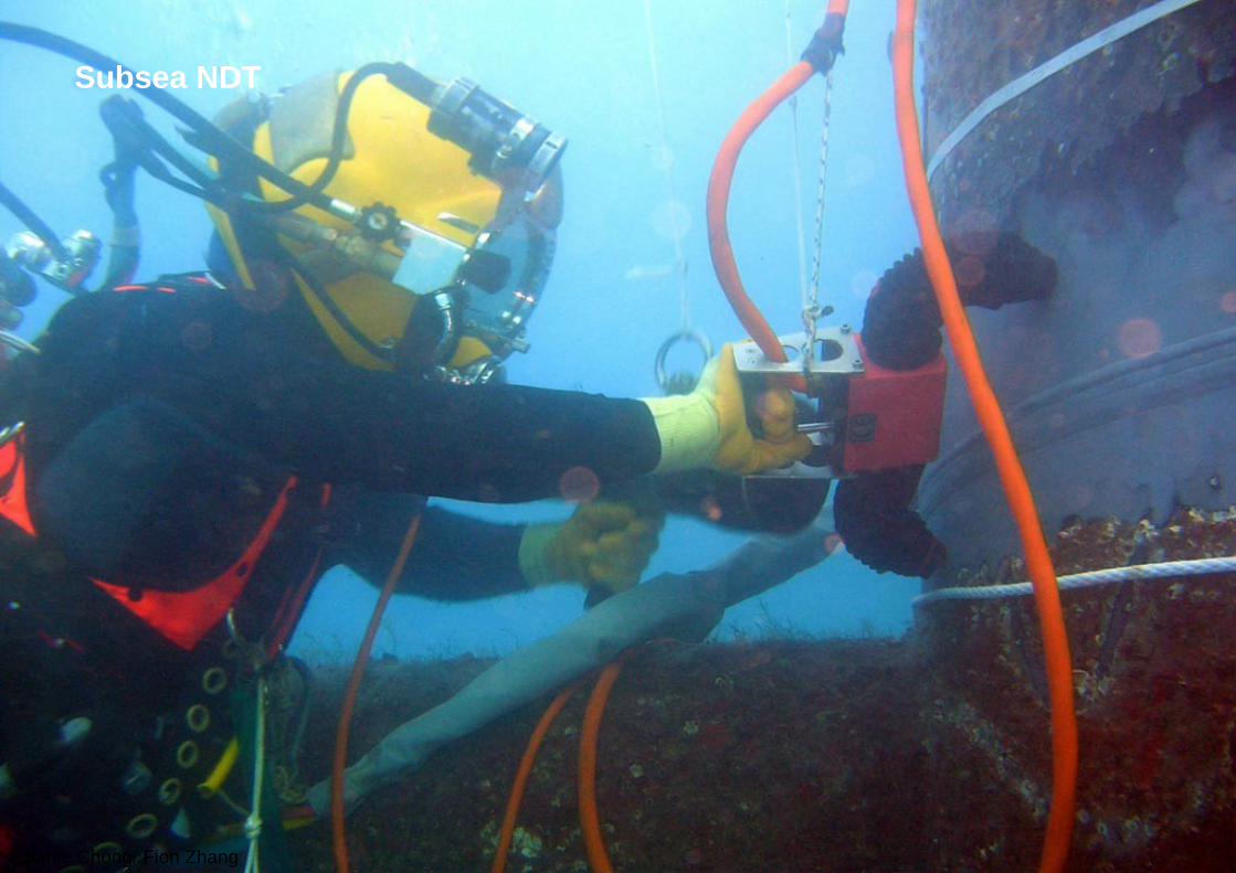
Subsea NDT
Charlie Chong/ Fion Zhang
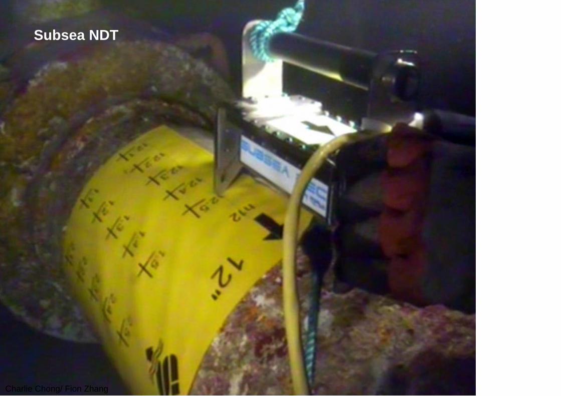
Subsea NDT
Charlie Chong/ Fion Zhang
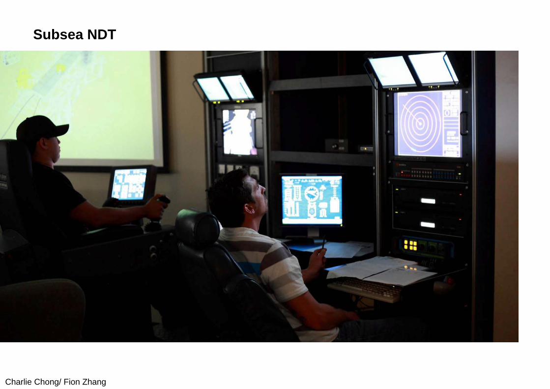
Subsea NDT
Charlie Chong/ Fion Zhang
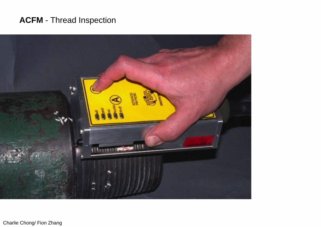
3. ACFM for Thread Inspection
Following the successful deployment of ACFM underwater, attention turned to other applications in the oil industry where the technique would be beneficial. One such application was the inspection of the threaded connections on drillpipe and other drillstring components. These are usually inspected by MPI (or dye-penetrant on non-magnetic tools), but this is difficult to do, especially on the female box threads, and it was known that MPI can miss defects in this situation, leading to the possibility of an expensive down-hole failure [3]. ACFM offered the advantages of a signal response that increased with defect depth (thus having a greater probability of not missing a significant defect), no need to carry out inspections in darkened areas, and no need to rotate the drillpipe. In addition, the relatively uniform geometry found in a thread meant that background signal changes are very small which allowed the development of software that could automate detection.
Charlie Chong/ Fion Zhang
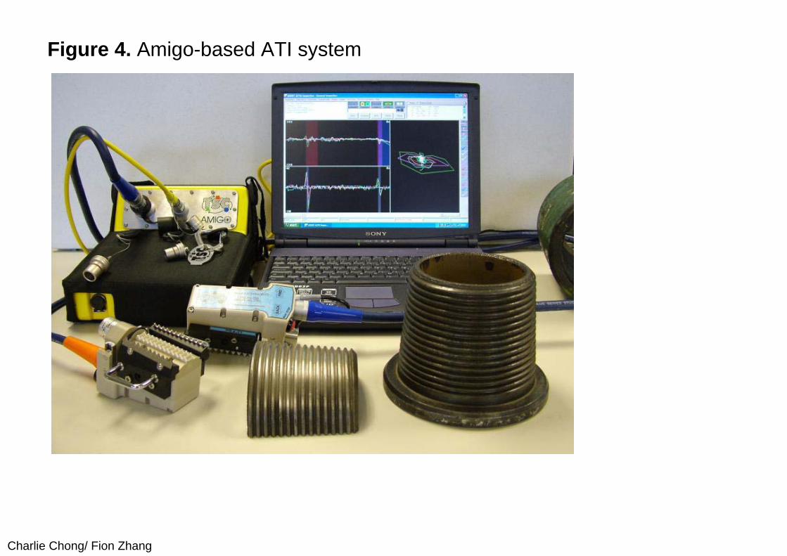
Thread inspection can be carried out with conventional single sensor probes, using replaceable shoes to fit each thread form. However, inspection speed can be greatly increased by using an array probe, with sensors in each thread root, which inspects the complete thread in one 360° scan.
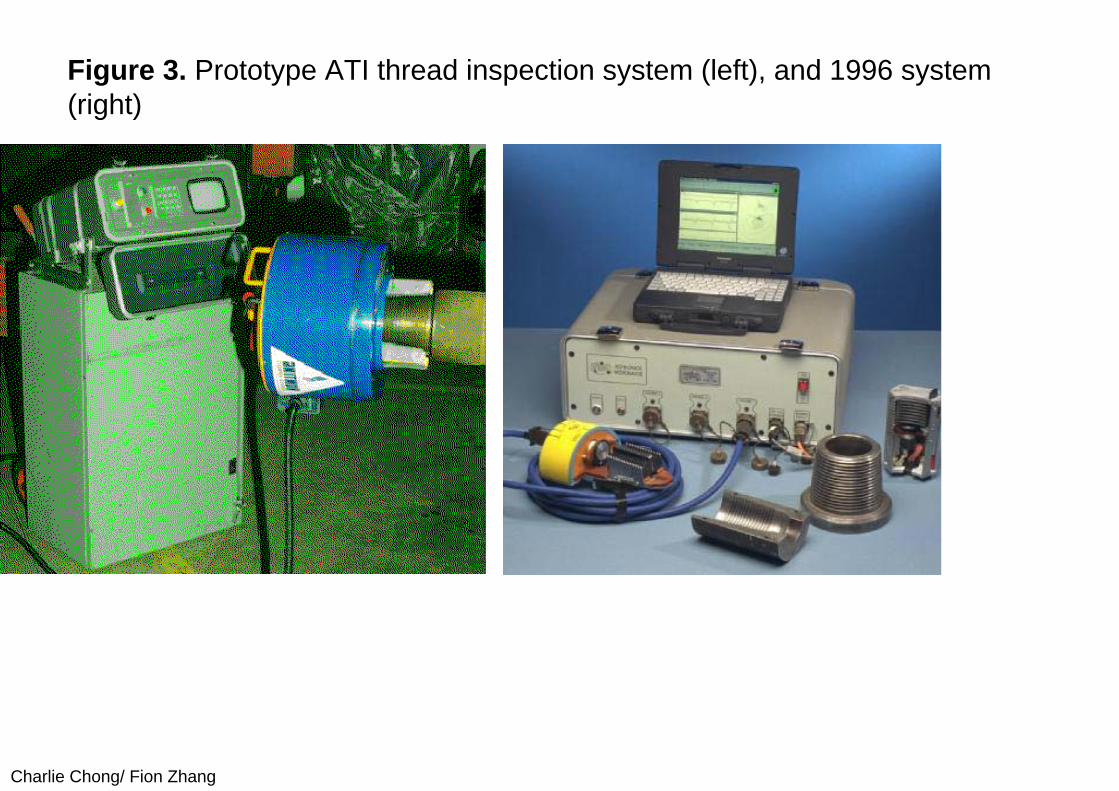
The first prototype array thread inspection system (known as Automated Thread Inspection, or ATI, shown on the left in Figure 3) was intended to be completely automated. It included proximity sensors to indicate when the inspection device was engaged properly on the first loaded thread, lift-off sensors to ensure probes sit down in the thread roots, and pneumatic drives to rotate the tool around the thread. The operator was just required to put the probe head on the tool joint, push a button to start the inspection, and take the head off at the end of the inspection. Two array probes were used so the tool only had to rotate 180°. However, the device proved very unwieldy不灵巧的 and difficult to deploy reliably.
Charlie Chong/ Fion Zhang
Figure 3. Prototype ATI thread inspection system (left), and 1996 system (right)
Charlie Chong/ Fion Zhang
It was decided to abandon the idea of making the system completely automated, and instead to require more from the operator. In 1996, a group of UK oil companies funded the development of a new ATI system based on the U12 ACFM instrument designed to support three different array probes at the same time. The operator was responsible for placing the probes in the right place, and for rotating the probe around the thread, avoiding the pneumatics and motors of the prototype system. Since no position information was available from a motor, each array probe contained a rotary position encoder to record defect locations and lengths. The minimum defect size for reliable automated detection and sizing was proven to meet the target size of 8mm long by 0.75mm deep, although defects as small as 5mm long by 0.5mm deep could usually be detected.
Charlie Chong/ Fion Zhang
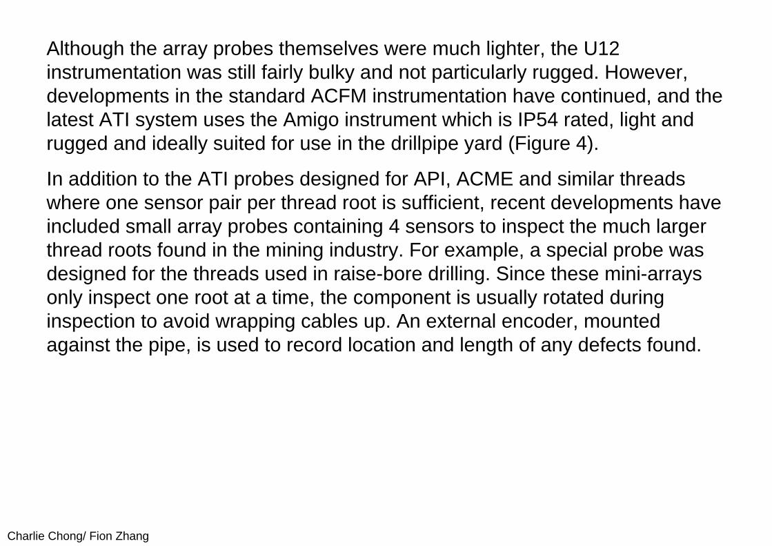
Although the array probes themselves were much lighter, the U12 instrumentation was still fairly bulky and not particularly rugged. However, developments in the standard ACFM instrumentation have continued, and the latest ATI system uses the Amigo instrument which is IP54 rated, light and rugged and ideally suited for use in the drillpipe yard (Figure 4).
In addition to the ATI probes designed for API, ACME and similar threads where one sensor pair per thread root is sufficient, recent developments have included small array probes containing 4 sensors to inspect the much larger thread roots found in the mining industry. For example, a special probe was designed for the threads used in raise-bore drilling. Since these mini-arrays only inspect one root at a time, the component is usually rotated during inspection to avoid wrapping cables up. An external encoder, mounted against the pipe, is used to record location and length of any defects found.
Charlie Chong/ Fion Zhang
Figure 4. Amigo-based ATI system
Charlie Chong/ Fion Zhang
ACFM - Thread Inspection
Charlie Chong/ Fion Zhang
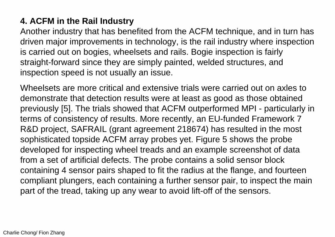
4. ACFM in the Rail IndustryAnother industry that has benefited from the ACFM technique, and in turn has driven major improvements in technology, is the rail industry where inspection is carried out on bogies, wheelsets and rails. Bogie inspection is fairly straight-forward since they are simply painted, welded structures, and inspection speed is not usually an issue.
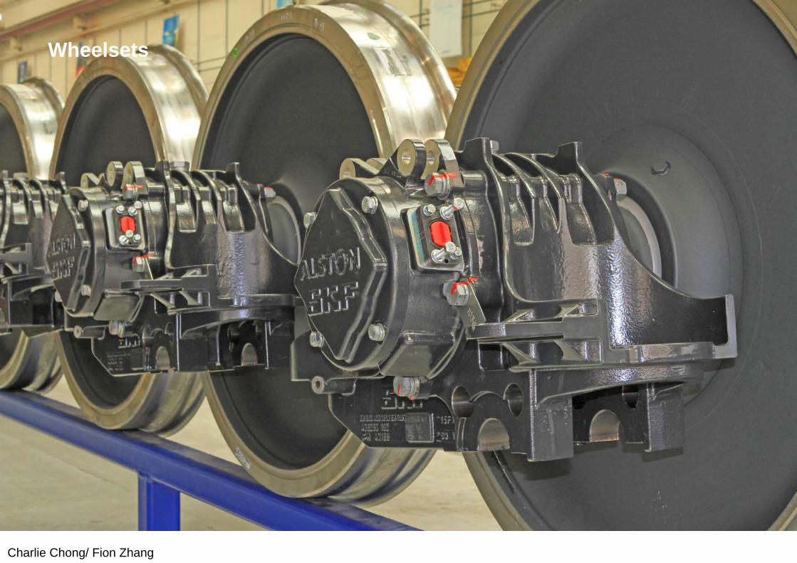
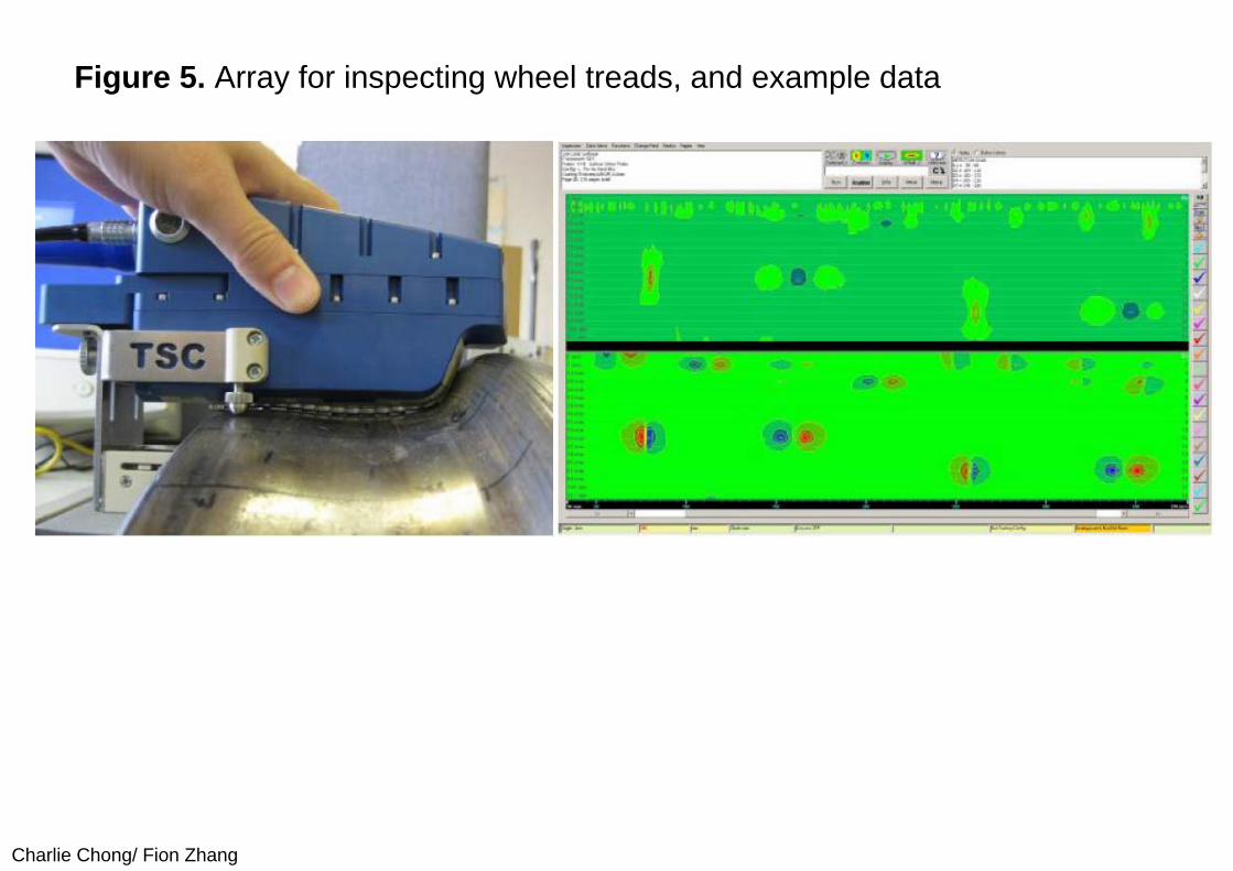
Wheelsets are more critical and extensive trials were carried out on axles to demonstrate that detection results were at least as good as those obtained previously [5]. The trials showed that ACFM outperformed MPI - particularly in terms of consistency of results. More recently, an EU-funded Framework 7 R&D project, SAFRAIL (grant agreement 218674) has resulted in the most sophisticated topside ACFM array probes yet. Figure 5 shows the probe developed for inspecting wheel treads and an example screenshot of data from a set of artificial defects. The probe contains a solid sensor block containing 4 sensor pairs shaped to fit the radius at the flange, and fourteen compliant plungers, each containing a further sensor pair, to inspect the main part of the tread, taking up any wear to avoid lift-off of the sensors.
Charlie Chong/ Fion Zhang
Wheelsets
Charlie Chong/ Fion Zhang
Following these successes, attention has turned to the sizing of rolling contact fatigue (RCF) cracks on rails. Rail breaks from RCF cracking, particularly on bends, was a major problem in the UK in the 1990s. Inspection was conventionally carried by visual inspection and ultrasonic “walking stick”probes. Visual inspection gives no indication of the depth of any defects seen, while there was concern that ultrasonic probes were not able to depth size the deepest defect if it was closely surrounded by shallower ones.
RCF defects have very different morphology to the standard fatigue cracks for which ACFM was developed. They are generally inclined at only 30o or so from the surface, but then may change direction to grow towards the surface leading to loss of part of the rail surface, or conversely may turn downwards rapidly through the rail leading to a rail break.
Charlie Chong/ Fion Zhang
In addition to this, the crack front will often be wider under the surface than the length on the surface, and crack depth will be large compared to surface length. All these factors mean that the theoretical sizing model developed in the 1980s does not work for RCF cracks. To overcome this, extensive calibration trials were undertaken using rail with real RCF cracks which were then broken open. Results of sizing using the new calibration procedure were subsequently compared with other defective rails and generally good agreement was found
Special software incorporating the new sizing algorithm was produced. This software also included automated detection, and reporting of the deepest defect found in a given length of rail. An ACFM array probe, shaped to the rail profile, was fitted to a “walking stick” that also carried a modified high-speed Amigo instrument and laptop. Further research is now underway to speed up the data throughput to allow deployment of ACFM on track vehicles such as road-rail cars and test trains, running at speeds between 15 and 100 km/hr.
Charlie Chong/ Fion Zhang
Figure 5. Array for inspecting wheel treads, and example data
Charlie Chong/ Fion Zhang
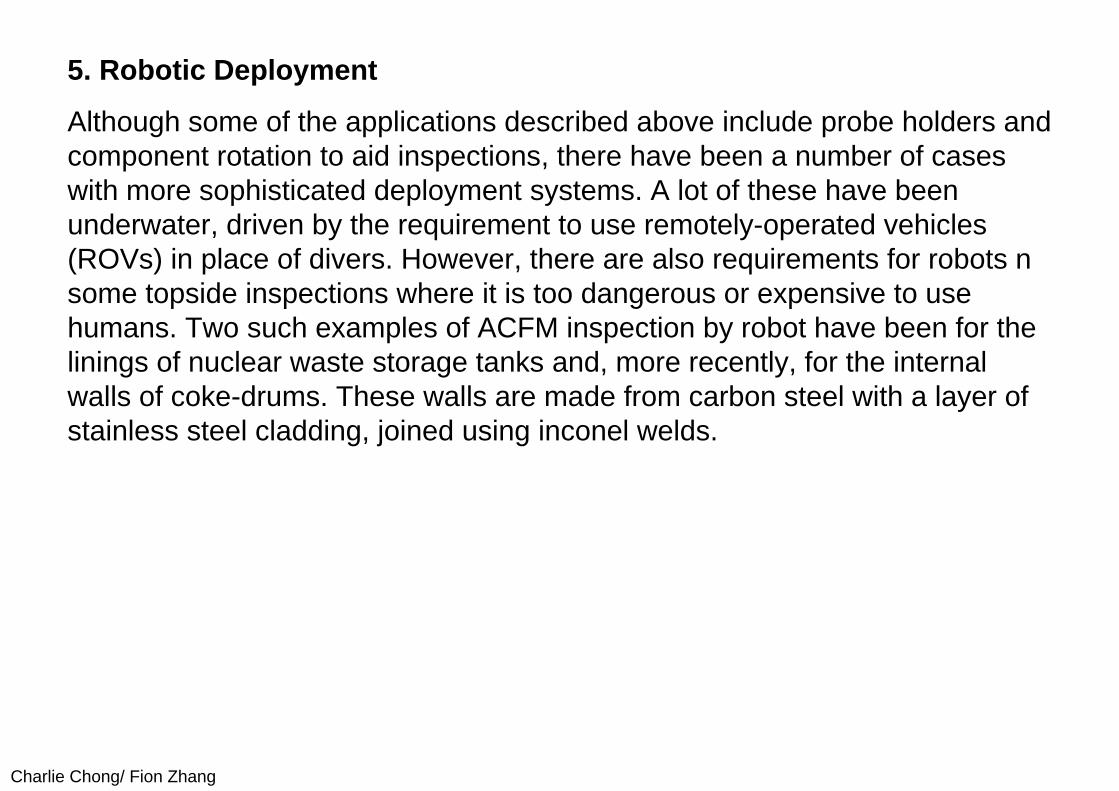
5. Robotic Deployment
Although some of the applications described above include probe holders and component rotation to aid inspections, there have been a number of cases with more sophisticated deployment systems. A lot of these have been underwater, driven by the requirement to use remotely-operated vehicles (ROVs) in place of divers. However, there are also requirements for robots n some topside inspections where it is too dangerous or expensive to use humans. Two such examples of ACFM inspection by robot have been for the linings of nuclear waste storage tanks and, more recently, for the internal walls of coke-drums. These walls are made from carbon steel with a layer of stainless steel cladding, joined using inconel welds.
Charlie Chong/ Fion Zhang
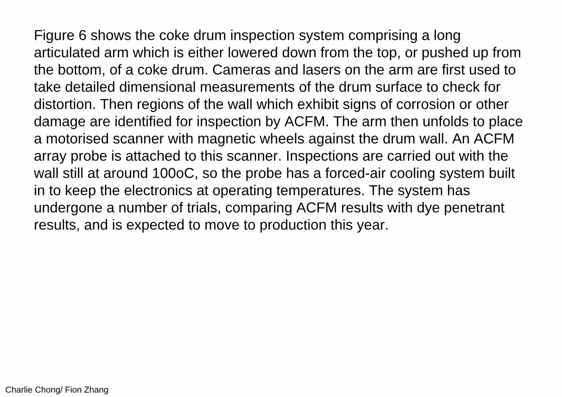
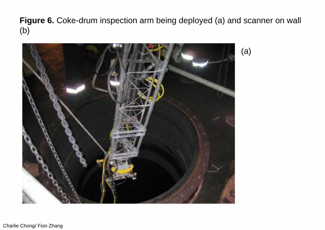
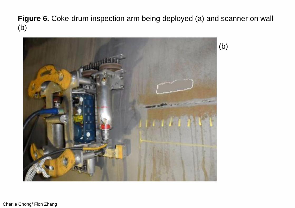
Figure 6 shows the coke drum inspection system comprising a longarticulated arm which is either lowered down from the top, or pushed up from the bottom, of a coke drum. Cameras and lasers on the arm are first used to take detailed dimensional measurements of the drum surface to check for distortion. Then regions of the wall which exhibit signs of corrosion or other damage are identified for inspection by ACFM. The arm then unfolds to place a motorised scanner with magnetic wheels against the drum wall. An ACFM array probe is attached to this scanner. Inspections are carried out with the wall still at around 100oC, so the probe has a forced-air cooling system built in to keep the electronics at operating temperatures. The system has undergone a number of trials, comparing ACFM results with dye penetrant results, and is expected to move to production this year.
Charlie Chong/ Fion Zhang
Figure 6. Coke-drum inspection arm being deployed (a) and scanner on wall (b)
(a)
Charlie Chong/ Fion Zhang
Figure 6. Coke-drum inspection arm being deployed (a) and scanner on wall (b)
(b)
Charlie Chong/ Fion Zhang
6. Conclusions
Since the first commercial systems became available 20 years ago, ACFM has continued to evolve to solve inspection problems in a wide variety of industries. Instrumentation continues to get smaller and faster, array probes get larger, and deployment systems get more sophisticated. It is expected that this trend will continue.
Charlie Chong/ Fion Zhang
Reading 3: TSC Inspection Systems ACFM Inspection Procedure QFMu and U31
(I) Interpretation of ACFM Signals1. General MethodIn general, a defect will product a characteristic signal on Bx and Bz signals and these combine to give the "butterfly". The rule adopted is that the signal represents a defect when:
1) Bz responds by a peak and trough, and2) Bx responds by a "dip" from the mean value.
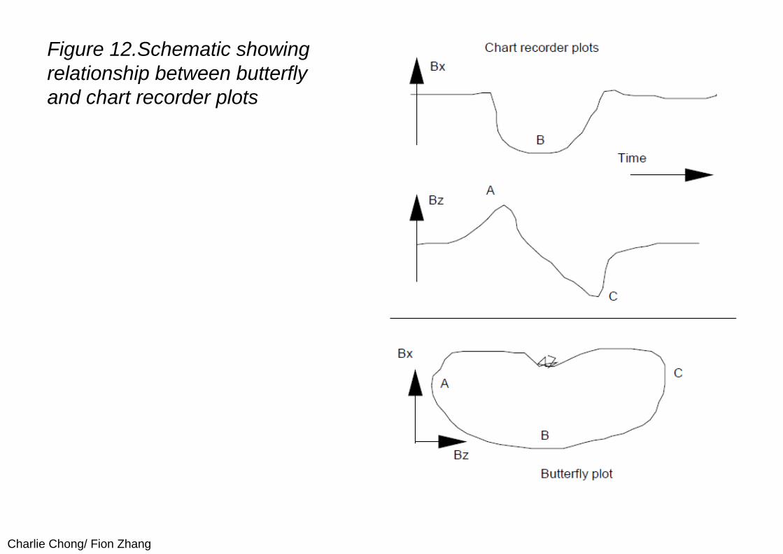
In the majority of situations for, isolated and relatively short cracks, this will give a butterfly plot which moves to right or left (according to probe direction), then downward then returns to the original position to close the loop. Figure 12 The figure below shows the relationship between Bx, Bz and the butterfly trace where "A" represents the first Bz peak, "B" represents the deepest point in Bx, and "C" represents the Bz trough.
http://erikatchison.com/userfiles/file/Documents/ACFM%20Inspection%20Procedure.pdf
Charlie Chong/ Fion Zhang
Figure 12.Schematic showing relationship between butterfly and chart recorder plots
Charlie Chong/ Fion Zhang
Lift off, permeability changes, probe rocking etc. can cause responses from Bx and or Bz. Lift-off, for example, causes the Bx signal to dip or peak (depending on material type) with little response from the Bz signal. This would produce a closed loop confined to the vertical axis rather than the open loop produced by a crack. A seam weld, on the other hand, usually causes a peak in Bx combined with Bz signals that result in an open loop moving upwards from the starting point.
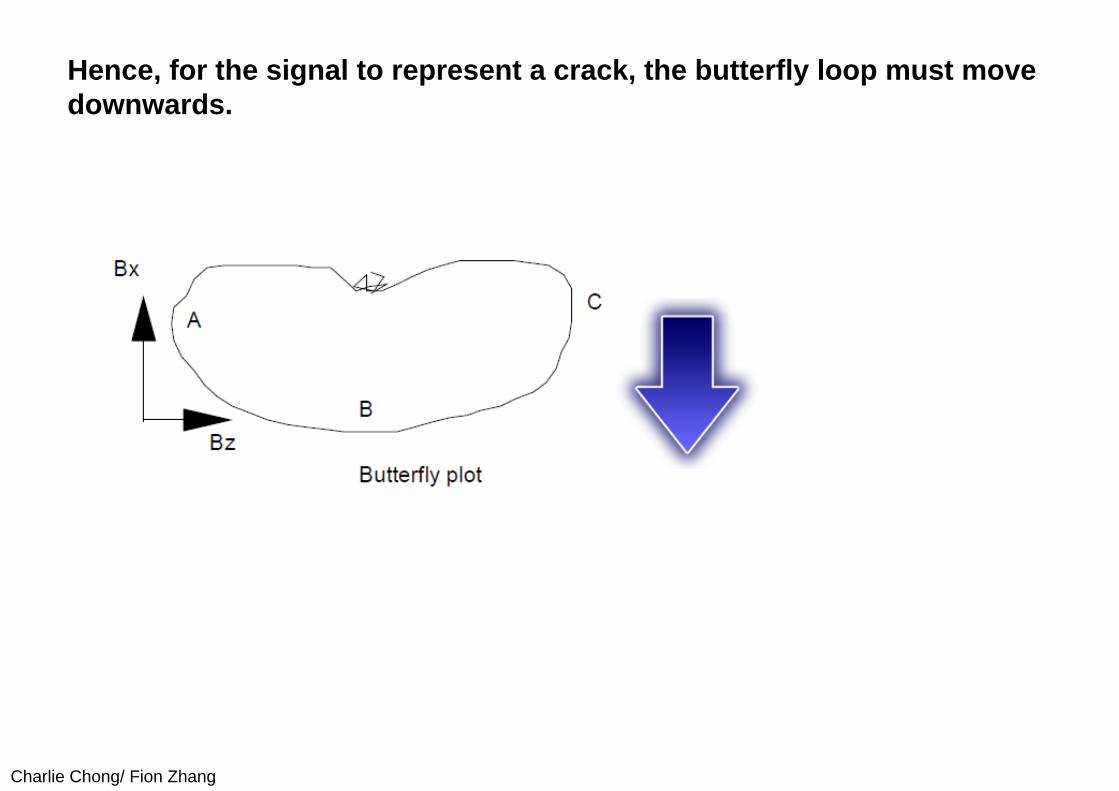
Hence, for the signal to represent a crack, the butterfly loop must move downwards. This rule is intended to eliminate false calls due to momentary lift off, perhaps as the probe runs over local weld imperfections. It therefore is intended for small signals. There are exceptions to the general rules and these mainly apply to long defects (> 50mm).
Keywords:Hence, for the signal to represent a crack, the butterfly loop must move downwards.
Charlie Chong/ Fion Zhang
Hence, for the signal to represent a crack, the butterfly loop must move downwards.
Charlie Chong/ Fion Zhang
For long cracks the Bz peak and trough may be some way apart. This means hat at the centre of the crack there is no Bz signal and we rely on Bx (i.e. the dip in Bx) to make the butterfly go down. If there is a general drift on the Bx signal, i.e. if the top signal is not perfectly level, this may confuse the butterfly by acting against the crack signal. This conflicting Bx signal means the butterfly rules no longer can be relied on and it is necessary to use the Bx and Bz plots to look for tell-tale signals where there is a response from Bz followed by a downward deviation, from the trend, on Bx. This is particularly important for tight angles where the Bx signal trend rises toward the tight angle due to global geometry effects.
In theory it is possible for a weld to be cracked around the full circumference, thus resulting in no crack ends. If the crack has a uniform depth, the Bx signals would be lower than expected, but in all other aspects the signals could be similar to an uncracked connection. In this situation the presence of a signal centred much lower on the butterfly plot than for other connections should be an indication that a full circumference defect is present. This can be further investigated by comparing the Bx signals as the probe is moved from parent plate to the weld toe area and then repeating the exercise on the other weld toe.
Charlie Chong/ Fion Zhang
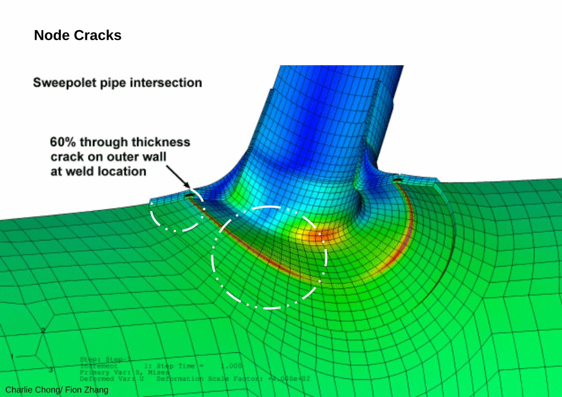
Node Cracks
Charlie Chong/ Fion Zhang
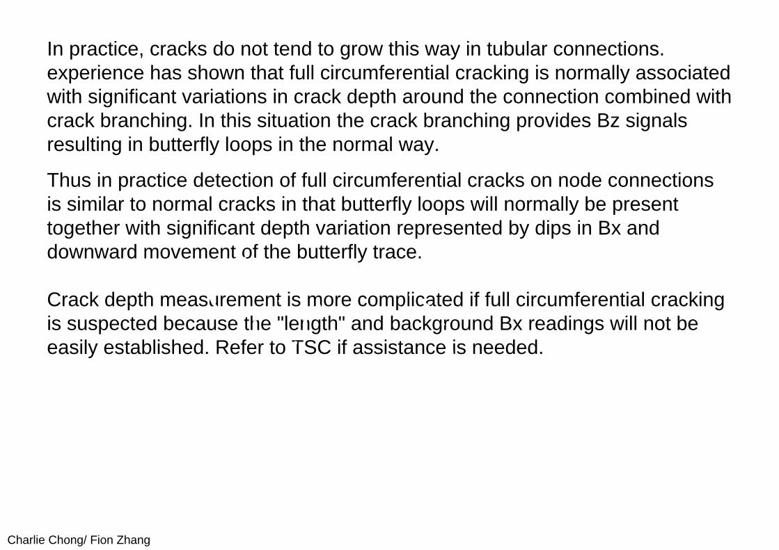
In practice, cracks do not tend to grow this way in tubular connections. experience has shown that full circumferential cracking is normally associated with significant variations in crack depth around the connection combined with crack branching. In this situation the crack branching provides Bz signals resulting in butterfly loops in the normal way.
Thus in practice detection of full circumferential cracks on node connections is similar to normal cracks in that butterfly loops will normally be present together with significant depth variation represented by dips in Bx and downward movement of the butterfly trace.
Crack depth measurement is more complicated if full circumferential cracking is suspected because the "length" and background Bx readings will not be easily established. Refer to TSC if assistance is needed.
Charlie Chong/ Fion Zhang
At all times look at the Bx and Bz traces. If Bx has a dip then suspect a crack. If the butterfly makes any significant loops, look at a broad area either side of the signal. This is particularly important if the butterfly is moving up or down the screen. A butterfly moving up or down the screen with any sort of looping is likely to be a long crack.
Charlie Chong/ Fion Zhang
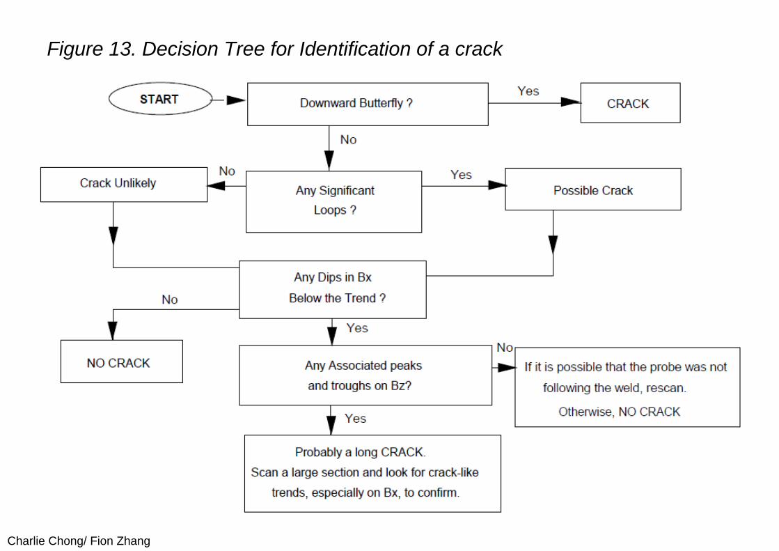
Figure 13. Decision Tree for Identification of a crack
Charlie Chong/ Fion Zhang
2. Crack SizingCrack sizing can be carried out either on-line (immediately after the necessary data has been collected) or offline (by recalling stored data). During the detection stage, scans of Bx and Bz are recorded for all defects found. A first estimate of length is also obtained from a manual measurement of the extent of the Bz signal. This data is then used to obtain sizing estimates using the QFMu program as outlined below. For more details, refer to the Level 1 Software User Manual.
Charlie Chong/ Fion Zhang
1. Select a section of the Bx time base plot to one side of the defect signal that is representative of the background level. This should simultaneously be near the centre of the area filled bay the general off crack background noise in the butterfly plot. This value is chosen as the Bx Background Level. N.B. If the background level is significantly different either side of the defect, the average of the two values should be used. This is normally necessary for defects in regions of changing geometry or near to a plate edge (see Inspecting Flat Plate Welded Supports/Stiffeners).
2. Select the minimum of the Bx time base trace from the centre of the defect signal (or the bottom of the butterfly loop). This value is chosen as the Bx Minimum Level.
3. To calculate defect length and depth, the QFMu software requires three parameters - the two Bx values selected above, and the length estimate obtained during the detection stage (the length in mm between the Bzpeak and trough indications at the inspection site).
Charlie Chong/ Fion Zhang
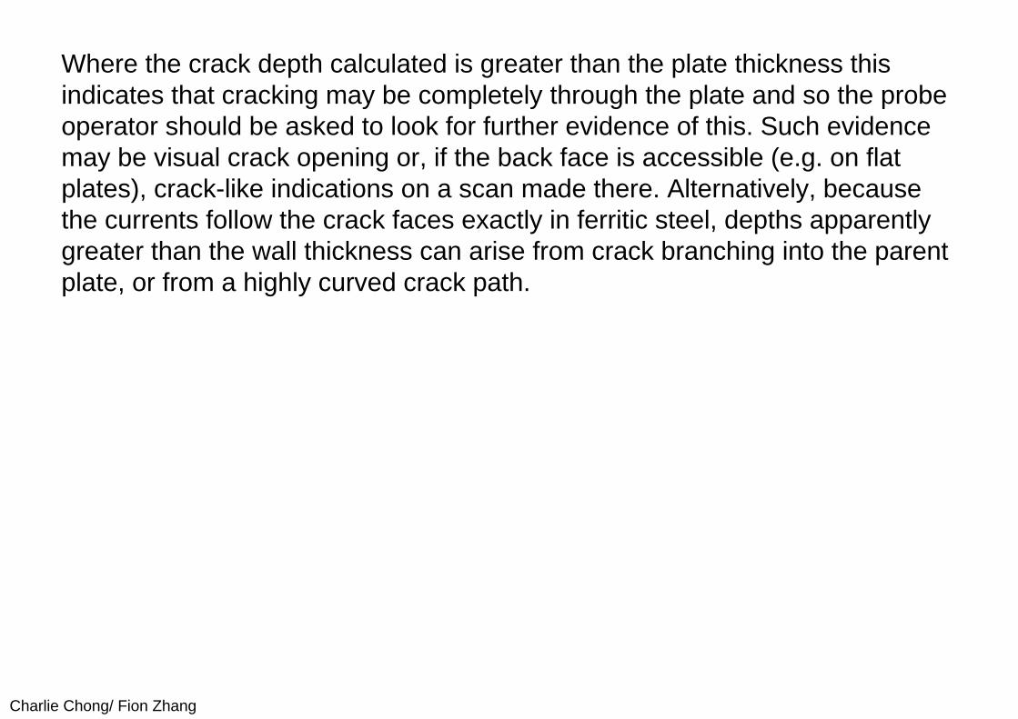
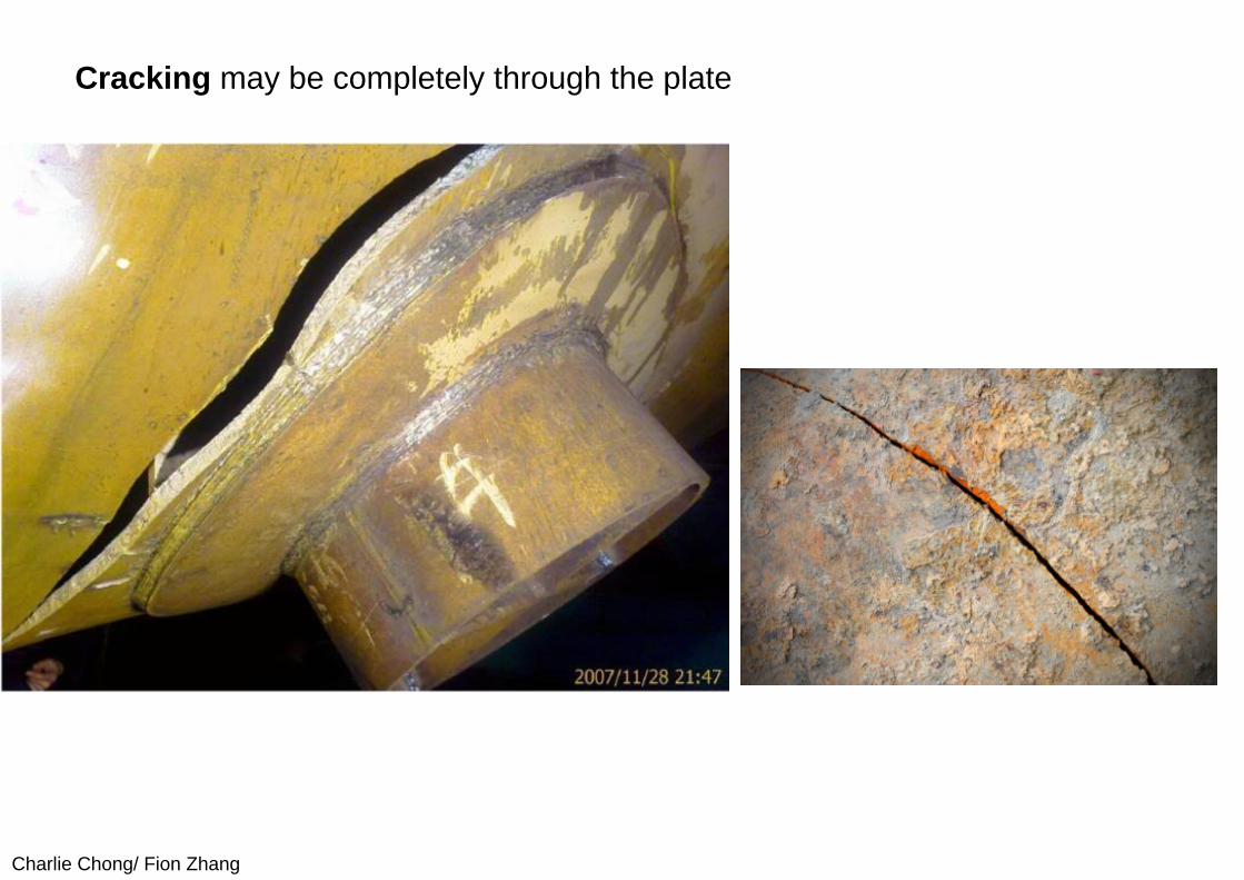
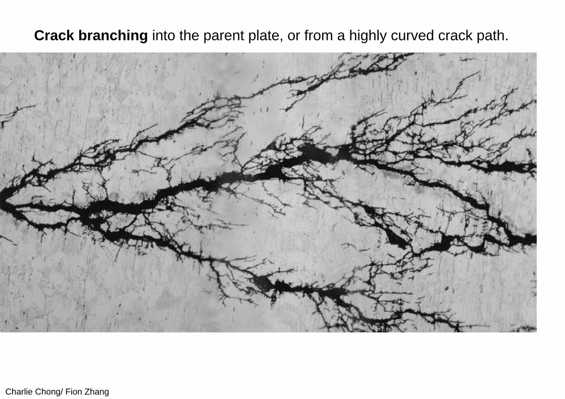
Where the crack depth calculated is greater than the plate thickness this indicates that cracking may be completely through the plate and so the probe operator should be asked to look for further evidence of this. Such evidence may be visual crack opening or, if the back face is accessible (e.g. on flat plates), crack-like indications on a scan made there. Alternatively, because the currents follow the crack faces exactly in ferritic steel, depths apparently greater than the wall thickness can arise from crack branching into the parent plate, or from a highly curved crack path.
Charlie Chong/ Fion Zhang
Cracking may be completely through the plate
Charlie Chong/ Fion Zhang
Crack branching into the parent plate, or from a highly curved crack path.
Charlie Chong/ Fion Zhang
3. Using MPI With ACFMWhen defects are being removed by grinding, it is often the case that MPI is used in conjunction with ACFM to monitor defect removal. In these cases it is tempting to save inspection time by using MPI lengths instead of Bz lengths when sizing defects. This will lead to errors and is not a recommended practice. This section considers the implication and suggests how, under certain conditions, data from MPI inspection can be used in the absence of any additional information. When conducting MPI inspections an approved MPI inspection procedure should be used. Demagnetise the area following MPI inspection (see "Magnetic State" on page 15).
Charlie Chong/ Fion Zhang
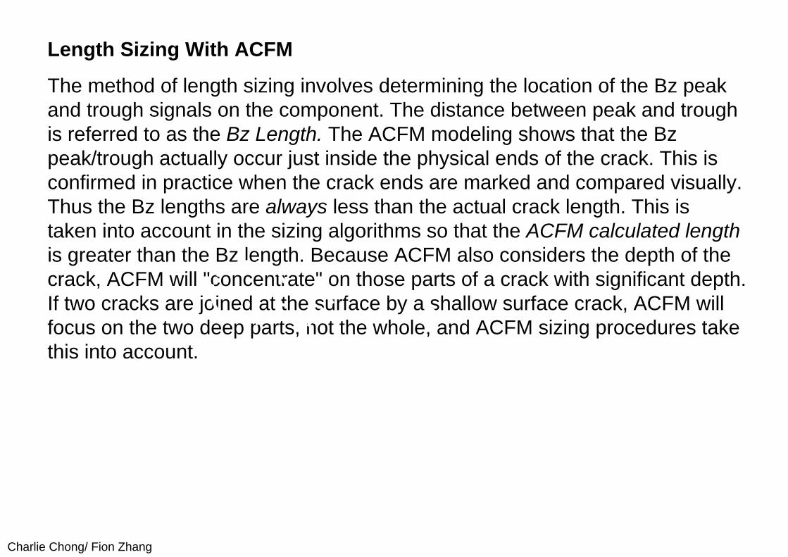
Length Sizing With ACFM
The method of length sizing involves determining the location of the Bz peak and trough signals on the component. The distance between peak and trough is referred to as the Bz Length. The ACFM modeling shows that the Bzpeak/trough actually occur just inside the physical ends of the crack. This is confirmed in practice when the crack ends are marked and compared visually. Thus the Bz lengths are always less than the actual crack length. This is taken into account in the sizing algorithms so that the ACFM calculated length is greater than the Bz length. Because ACFM also considers the depth of the crack, ACFM will "concentrate" on those parts of a crack with significant depth. If two cracks are joined at the surface by a shallow surface crack, ACFM will focus on the two deep parts, not the whole, and ACFM sizing procedures take this into account.
Charlie Chong/ Fion Zhang
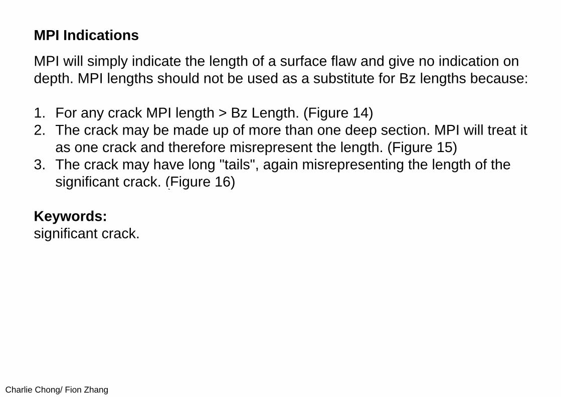
MPI Indications
MPI will simply indicate the length of a surface flaw and give no indication on depth. MPI lengths should not be used as a substitute for Bz lengths because:
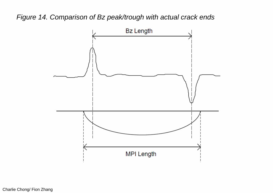
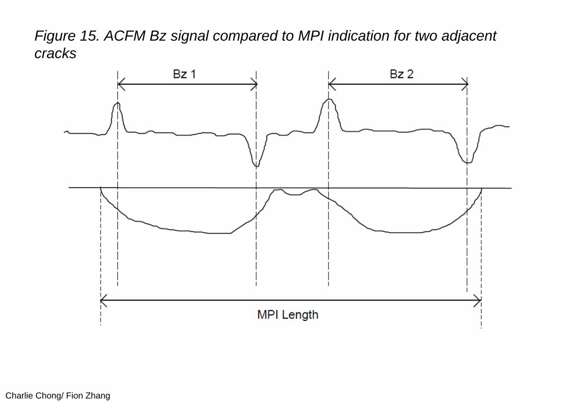
1. For any crack MPI length > Bz Length. (Figure 14)2. The crack may be made up of more than one deep section. MPI will treat it
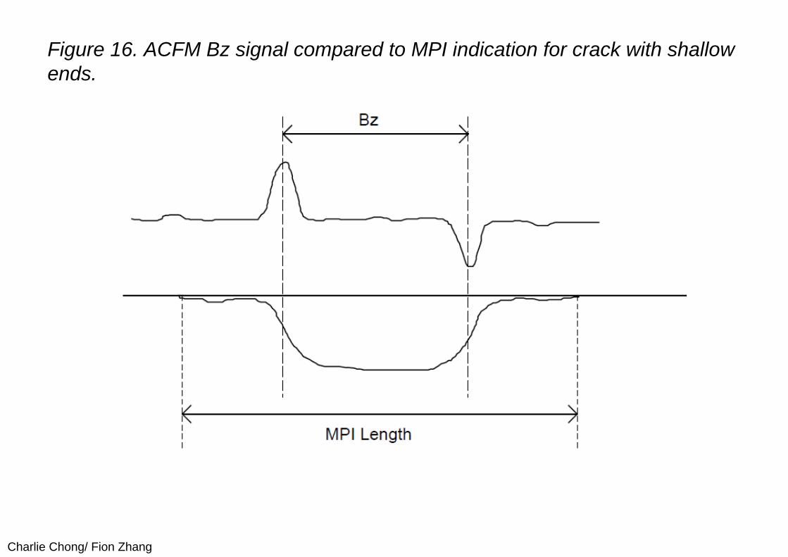
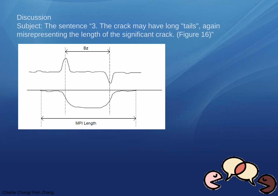
as one crack and therefore misrepresent the length. (Figure 15)3. The crack may have long "tails", again misrepresenting the length of the
significant crack. (Figure 16)
Keywords:significant crack.
Charlie Chong/ Fion Zhang
Figure 14. Comparison of Bz peak/trough with actual crack ends
Charlie Chong/ Fion Zhang
Figure 15. ACFM Bz signal compared to MPI indication for two adjacent cracks
Charlie Chong/ Fion Zhang
Figure 16. ACFM Bz signal compared to MPI indication for crack with shallow ends.
Charlie Chong/ Fion Zhang
DiscussionSubject: The sentence “3. The crack may have long "tails", again misrepresenting the length of the significant crack. (Figure 16)”
Charlie Chong/ Fion Zhang
4. Use of MPI Lengths In ACFM CalculationsOne example where it may be preferable to use MPI lengths instead of Bzlengths is a situation where ACFM is being used during a grinding process and it is found that there is a start/stop Bz signal at the grind profile ends which are close to the defect ends. Hence there may be some doubt as to whether the crack Bz locations are being masked by the grind profile end signals. As an alternative, MPI lengths may be used in the crack depth sizing. As described earlier, the use of MPI length as a substitute for Bz length is incorrect. However there is a work around if, and only if, certain criteria are met. The answer will still be approximate but may be acceptable.
Charlie Chong/ Fion Zhang
The criteria are:
1. Before grinding, carry out an ACFM inspection and use Bz to calculate the crack length. If:
i) The calculated length agrees with the MPI length, andii) The Bx signal indicates a simple crack continue to step 2. If either of
these conditions are not satisfied, do not attempt to use MPI information with ACFM.
2. Estimate by how much the Bz length is less than MPI. You should find that the Bz length is between 80% and 90% of MPI length.
3. Carry out the grinding.
Charlie Chong/ Fion Zhang
4. Re-inspect with ACFM. If the crack remains a single crack (i.e. no additional features appear on Bx take the MPI length after grinding and apply the factor in (2) above. Then compare the estimated ACFM length with the factored MPI length. If they agree, the factored MPI length should give a reasonable depth estimate when used in the ACFM sizing procedure. If the two estimates do not agree, it is possible that a situation such as shown in Figure 12 has arisen and the MPI length should not be used to depth size the defect.
5. The above process can be repeated providing the crack remains as a single defect. Should it split into two, the process will not work and any depth calculation will be in error.
Charlie Chong/ Fion Zhang
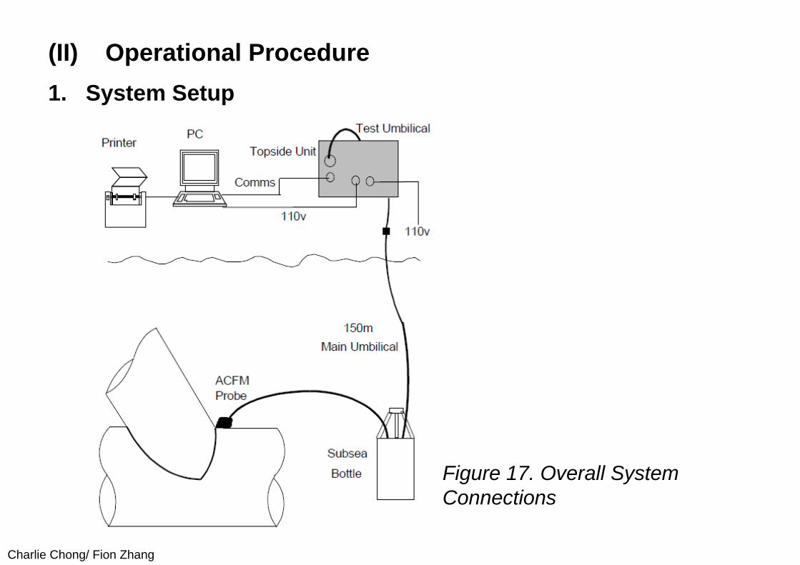
(II) Operational Procedure1. System Setup
Figure 17. Overall System Connections
Charlie Chong/ Fion Zhang
2. U31 Subsea Bottle
The U31 subsea bottle is designed to be deployed underwater with the diver. An ACFM probe is attached to the bottle via the 16 way Wetcon Connector. This connector may be broken subsea, to change probes for instance, but the bottle should be powered down first to prevent accelerated corrosion of the pins. Note that there is no shock hazard to the diver. An umbilical is connected to the 8 way Wetcon connector which carries power and communications to the bottle. The main umbilical is 150m long as standard but two may be joined together to give a 300m total length. Note that no more than two main umbilicals can be connected together. The main umbilical is deployed from the surface and attaches to the test umbilical which in turn is connected to the Topside Unit.
Charlie Chong/ Fion Zhang
3. U31 Topside UnitThe topside unit provides power and communications to the subsea bottle. The test umbilical is connected to the 12 way Amphenol connector on the front panel. This umbilical can then be plugged directly into the subsea bottle for testing purposes or routed to a convenient location and attached to the main umbilical. 110V power is supplied to the unit via the 4 way Amphenol connector on the front panel. If the local supply is 240V then a suitable transformer will be required. Note that unlike previous underwater ACFM instruments the U31 does not require a centre tapped isolation transformer. A 110V output connector is supplied on the front panel to power the computer. The topside unit is connected to the computer via a communications cable which is attached to the 6 way Lemo connector on the front panel.
Charlie Chong/ Fion Zhang
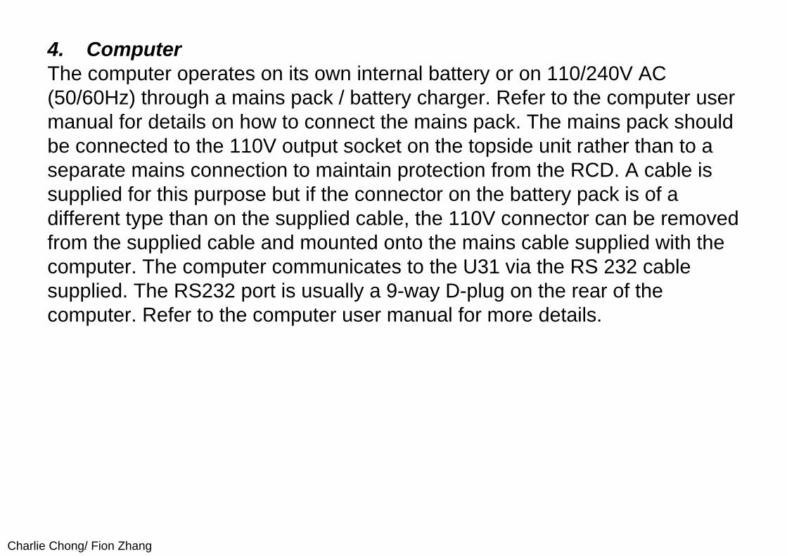
4. ComputerThe computer operates on its own internal battery or on 110/240V AC (50/60Hz) through a mains pack / battery charger. Refer to the computer user manual for details on how to connect the mains pack. The mains pack should be connected to the 110V output socket on the topside unit rather than to a separate mains connection to maintain protection from the RCD. A cable is supplied for this purpose but if the connector on the battery pack is of a different type than on the supplied cable, the 110V connector can be removed from the supplied cable and mounted onto the mains cable supplied with the computer. The computer communicates to the U31 via the RS 232 cable supplied. The RS232 port is usually a 9-way D-plug on the rear of the computer. Refer to the computer user manual for more details.
Charlie Chong/ Fion Zhang
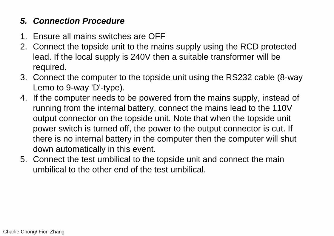
5. Connection Procedure
1. Ensure all mains switches are OFF2. Connect the topside unit to the mains supply using the RCD protected
lead. If the local supply is 240V then a suitable transformer will be required.
3. Connect the computer to the topside unit using the RS232 cable (8-way Lemo to 9-way 'D'-type).
4. If the computer needs to be powered from the mains supply, instead of running from the internal battery, connect the mains lead to the 110V output connector on the topside unit. Note that when the topside unit power switch is turned off, the power to the output connector is cut. If there is no internal battery in the computer then the computer will shut down automatically in this event.
5. Connect the test umbilical to the topside unit and connect the main umbilical to the other end of the test umbilical.

Charlie Chong/ Fion Zhang
6. Connect the main umbilical to the subsea bottle. 7. Test RCD by turning ON the mains supply to the lead (with the topside
unit still switched OFF). Press the Reset button and verify that the red indicator is showing. Press the Test button and confirm that the red indicator is removed. Press the Reset button again and check that the red indicator reappears and remains.
Charlie Chong/ Fion Zhang
6. Function CheckAt the start and end of an inspection session a function check must be performed using the equipment. This is to ensure that the equipment is functioning correctly and to familiarize the operator with the relative levels of noise and defect signal. The following procedure assumes familiarization with the QFMu software. For details, refer to the appropriate Software User Manuals.
Charlie Chong/ Fion Zhang
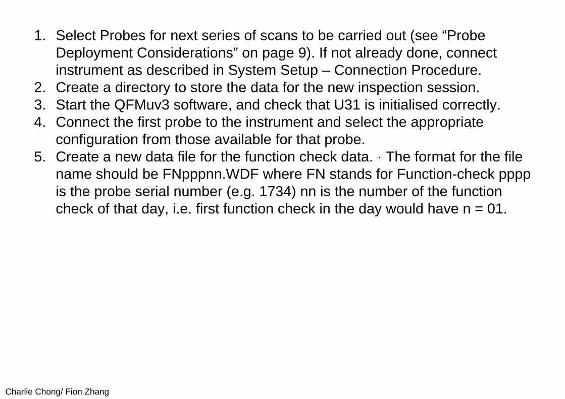
1. Select Probes for next series of scans to be carried out (see “Probe Deployment Considerations” on page 9). If not already done, connect instrument as described in System Setup – Connection Procedure.
2. Create a directory to store the data for the new inspection session. 3. Start the QFMuv3 software, and check that U31 is initialised correctly. 4. Connect the first probe to the instrument and select the appropriate
configuration from those available for that probe. 5. Create a new data file for the function check data. · The format for the file
name should be FNpppnn.WDF where FN stands for Function-check ppppis the probe serial number (e.g. 1734) nn is the number of the function check of that day, i.e. first function check in the day would have n = 01.
Charlie Chong/ Fion Zhang
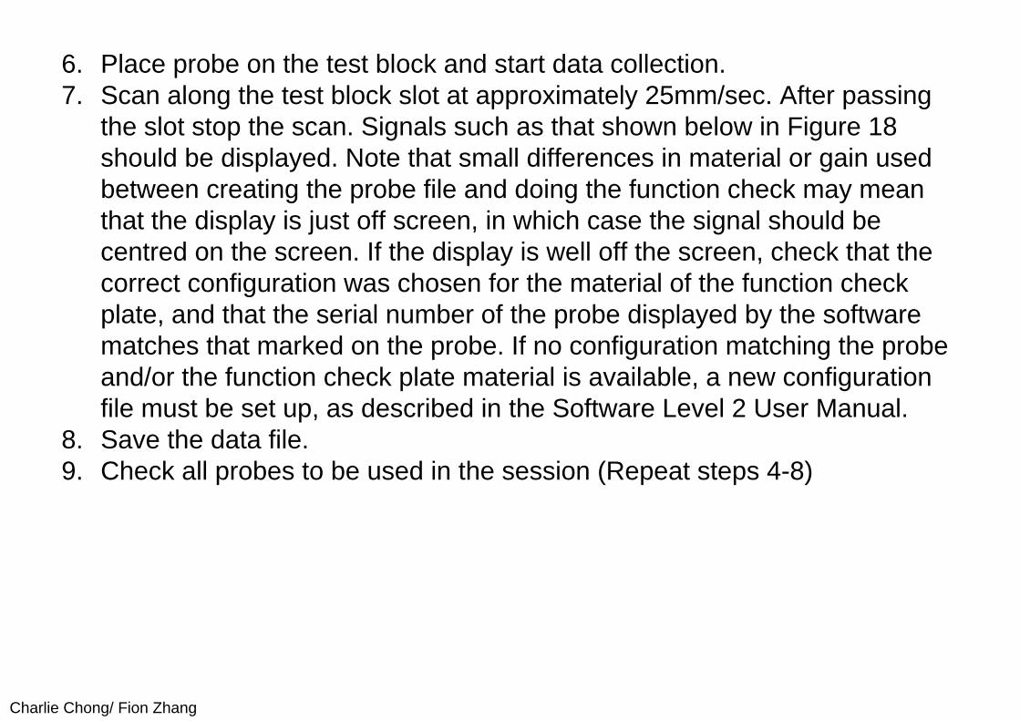
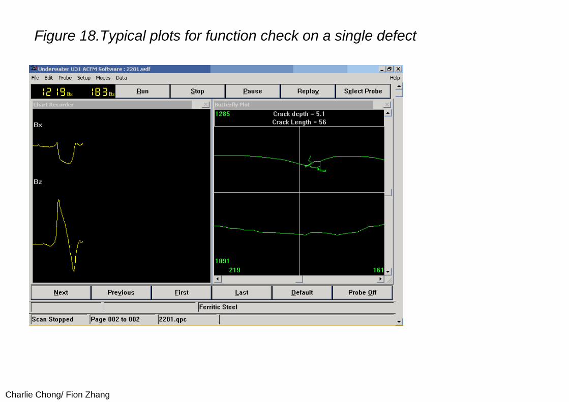
6. Place probe on the test block and start data collection. 7. Scan along the test block slot at approximately 25mm/sec. After passing
the slot stop the scan. Signals such as that shown below in Figure 18 should be displayed. Note that small differences in material or gain used between creating the probe file and doing the function check may mean that the display is just off screen, in which case the signal should be centred on the screen. If the display is well off the screen, check that the correct configuration was chosen for the material of the function check plate, and that the serial number of the probe displayed by the software matches that marked on the probe. If no configuration matching the probe and/or the function check plate material is available, a new configuration file must be set up, as described in the Software Level 2 User Manual.
8. Save the data file. 9. Check all probes to be used in the session (Repeat steps 4-8)
Charlie Chong/ Fion Zhang
Figure 18.Typical plots for function check on a single defect
Charlie Chong/ Fion Zhang
(III) Inspection Procedure
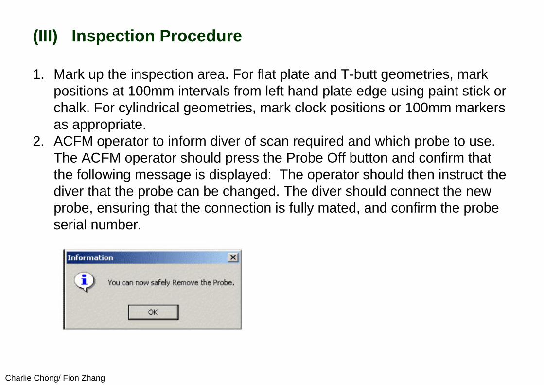
1. Mark up the inspection area. For flat plate and T-butt geometries, mark positions at 100mm intervals from left hand plate edge using paint stick or chalk. For cylindrical geometries, mark clock positions or 100mm markers as appropriate.
2. ACFM operator to inform diver of scan required and which probe to use. The ACFM operator should press the Probe Off button and confirm that the following message is displayed: The operator should then instruct the diver that the probe can be changed. The diver should connect the new probe, ensuring that the connection is fully mated, and confirm the probe serial number.
Charlie Chong/ Fion Zhang
3. When the diver has completed connecting the new probe, press the Select Probe button and select the required probe configuration. This will restore the power to the probe socket.
4. Create a new file for the inspection data. · Choose a filename in the form "XXXXXXXa“ where: XXXXXXX = Identifying code for location to be inspected (up to 7 characters). a = Inspection number/letter for that location (e.g. a for first inspection, b for second inspection etc.). When choosing a data filename, make sure the file is uniquely identifiable and contains a reference to the component under test. Note: The individual scans within the inspection are described by pages within the file, in numerical order. A separate recording sheet or log-book must record the scan made on each page (i.e. the weld toe/bead inspected and thedirection of the probe 'C' or 'A').
Charlie Chong/ Fion Zhang
5. Set the range of the numbered marker lines (or clock-points) to be covered in the scan (start, end and direction) While recording data, reference markers can be entered which are called CLOCK POINTS. These are lines labelled with a number between 1 and 99. The numbers wrap around at the end point so that they can be used to mark positions when scanning around a tubular geometry. The default end point is 12, appropriate for conventional clock positions around a circle, however the markers can just as easily be used to scale mark a linear geometry. e.g. each marker may represent 100mm increments.
6. The diver should place the probe at beginning of scan, and confirm intended probe direction (Probe marker A or C leading) to the ACFM operator. When A is leading, the loop produced by a defect in the butterfly plot should be traced in an anti-clockwise direction, when C is leading it should be clockwise.
Charlie Chong/ Fion Zhang
7. The ACFM operator should start the scan and instruct the diver to begin moving the probe. The scan speed should be approx. 25mm/sec, but if this needs to be reduced or increased for operational reasons, the data sampling rate should be set accordingly. Note that if scan rates are set too high that there is an increased chance of the diver not scanning the probe carefully along the weld line.
Charlie Chong/ Fion Zhang
8. The diver should report when the centre of the probe passes a marker. The ACFM operator logs his position. The diver should report visual indications such as seam welds, weld run overlap, weld spatter or grinding marks when these are encountered. The ACFM operator mayadd an un-numbered marker to log these.
9. When the desired section is scanned or the end of the data page is reached or the diver cannot comfortably continue, then the ACFM operator should stop the scan.
10. When the scan has stopped the diver may be remove the probe fromthe component.
11. Study the data, looking for any defect indications. For defect detection refer to “Interpretation of ACFM Signals” on page 21. Any defect signal is to be noted in the report sheets by the operator and the area marked by the probe operator.
Charlie Chong/ Fion Zhang
12. Continue scanning with a minimum of one clock position, or 100mmoverlap on each scan (e.g. clock positions 11-3, 2-6, 5-9, 8-12). Repeat steps 5 to 11 until scan area is covered. When defects are detected, additional scans are necessary in order to facilitate sizing. These are:
i) a slow scan to cover all defects within a region. ii) a scan or series of scans to locate the ACFM crack ends. In these
scans the ACFM operator will ask the diver to move the probe so that it coincides with the peaks and troughs of the Bz signals (usually easiest to observe on the butterfly plot). When the ACFM operator is satisfied that the probe is in the correct place, the diver should place a mark or magnetic arrow to mark the location. The marking will normally be aligned directly with the probe centre.Alternatively, if the access does not allow this, the trailing edge of the probe can be marked first with the position of the centre of the probe marked later.
Charlie Chong/ Fion Zhang
13. Save the collected data in the file selected at the beginning of this session.
14. The diver should place a ruler or tape on the specimen and read off crack end positions to the ACFM operator. The ACFM operator mustrecord this “Bz crack length” and the distance to a datum on the data sheet.
15. Repeat steps 1 to 14 for all inspection areas on the specimen. 16. Crack depth sizing can be carried out immediately, or at a later date, in
accordance with the procedure described in "Crack Sizing" on page 24.
Charlie Chong/ Fion Zhang
(IV) End Of Session Function Check And Backup1. Procedure
Post-Session Function CheckTo ensure that the system was functioning correctly during the session, the function check should be repeated on the appropriate sample at the end of the shift using the procedure outlined in "Function Check" on page 30, steps 3 to 9.
Charlie Chong/ Fion Zhang
Backup Procedure1. Mark back-up medium (e.g. floppy disc, magneto-optical disc, CD-R) with
files to be copied. 2. Put back-up medium in appropriate drive 3. Back-Up all files created in the inspection shift.
4. Exit QFMu and check backup (i) Exit QFMu: (ii) Check files are stored on the backup medium using (e.g.) Windows
Explorer (iii) Remove the backup medium from drive and write-protect (if applicable). 4.
Switch off all power.
Charlie Chong/ Fion Zhang
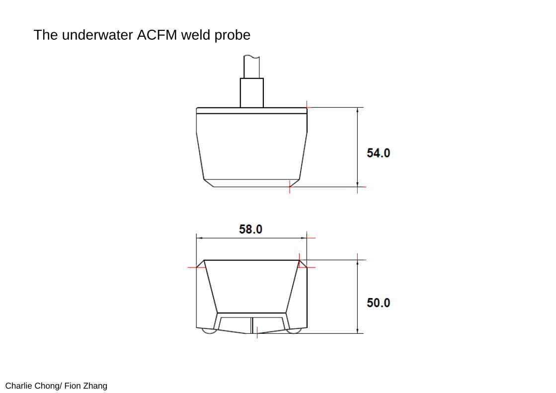
(V) Probe Specifications1. Underwater Weld ProbeThe Underwater Weld Probe is designed for subsea inspection of welds, plate and tubulars. The bottom face is fitted with two feet which, together with the wear-resistant probe nose housing the sensors, give a stable tripod arrangement for ease of scanning. The probe is sealed and fitted with a 50m cable. The probe electronics are encapsulated in a bulge in the cable about 30cm from the probe body. If the probe is to be used in an environment where sharp marine growth could easily damage the probe cable, it is recommended that the cable be protected using additional sheathing.
Charlie Chong/ Fion Zhang
The underwater ACFM weld probe
Charlie Chong/ Fion Zhang
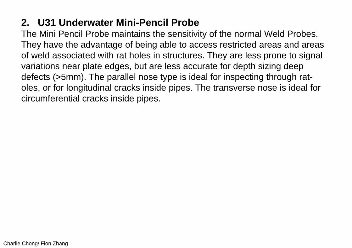
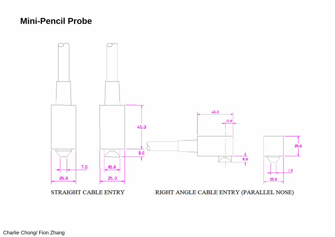
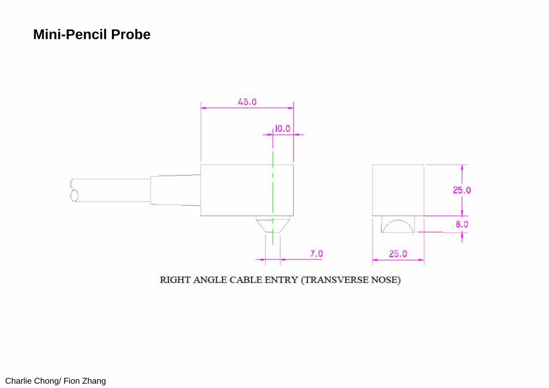
2. U31 Underwater Mini-Pencil ProbeThe Mini Pencil Probe maintains the sensitivity of the normal Weld Probes. They have the advantage of being able to access restricted areas and areas of weld associated with rat holes in structures. They are less prone to signal variations near plate edges, but are less accurate for depth sizing deep defects (>5mm). The parallel nose type is ideal for inspecting through rat-oles, or for longitudinal cracks inside pipes. The transverse nose is ideal for circumferential cracks inside pipes.
Charlie Chong/ Fion Zhang
Mini-Pencil Probe
Charlie Chong/ Fion Zhang
Mini-Pencil Probe
Charlie Chong/ Fion Zhang
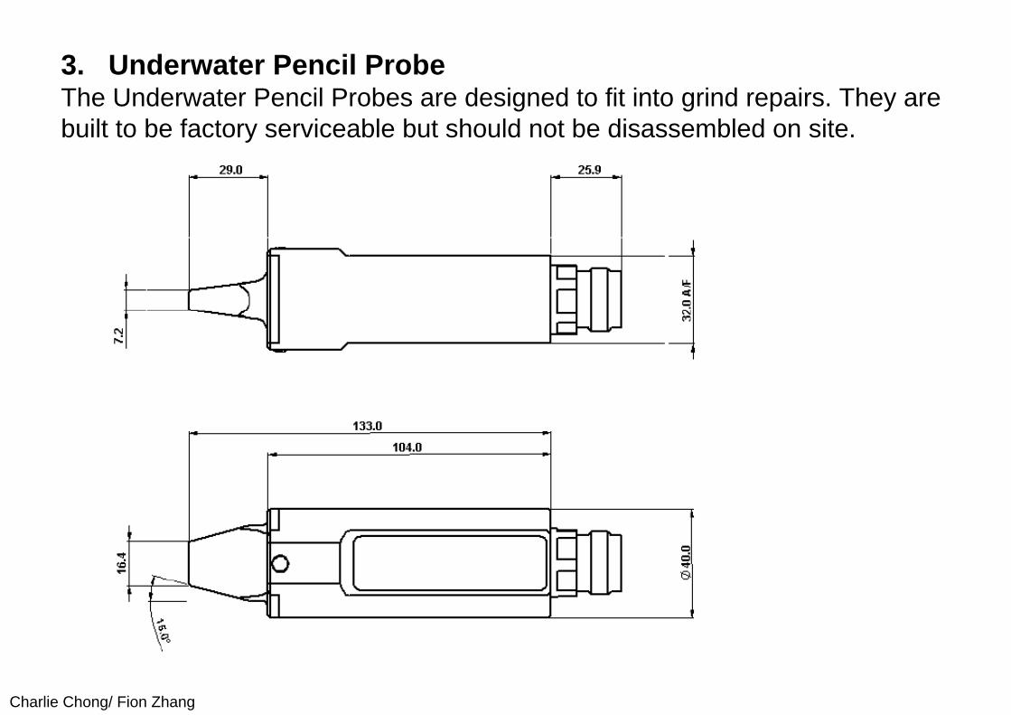
3. Underwater Pencil ProbeThe Underwater Pencil Probes are designed to fit into grind repairs. They are built to be factory serviceable but should not be disassembled on site.
Charlie Chong/ Fion Zhang
4. Other Probe TypesOther probe types may be introduced as part of TSC's continuing policy of product development. If a suitable probe for a particular application is not shown here, contact TSC.
Charlie Chong/ Fion Zhang
(VI) Purpose of Probe FilesThe aims of a probe file are:
a) To maintain a consistent detection sensitivity between inspections, and between probes.
b) To maintain sizing accuracy
The first aim is satisfied by the probe file containing graph scalings to give a standard size butterfly loop from a given defect. The second aim is atisfied by the probe file containing calculated values for inherent coil lift-off and sensitivity. If, after checking instrument settings etc., it is found that the issued probe file is unsuitable for a particular application (for example the inspection is not on ferritic steel or the readings are saturating), refer to TSC. If approval is given to create a new probe file on site, TSC will issue the appropriate procedure. It should be noted that to produce a new probe file, an function check plate in the same material as that under inspection will be needed, containing a slot (preferably 50mm long by 5mm deep).
Charlie Chong/ Fion Zhang
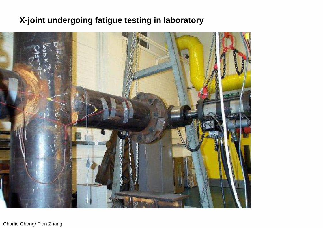
Reading 4: Crack Growth MonitoringWhat is monitoring, and why do it?Crack growth monitoring is where a sequence of crack depths and/or lengths are measured at the same point over a period of time. It is often used in a test laboratory to provide data on fatigue resistance of a material under given conditions (e.g. environment, load, geometry etc.).
In these tests the components can be standard defined geometries (such as compact tension or tensile test specimens) or small pieces representative of a larger structure (such as T-butt welds or tubular intersections). Crack monitoring can also be required on-site to give early warning of crack initiation in a critical area, for example, or to monitor a known defect up to the point where a failure may be imminent allowing repair to be scheduled at a convenient time (i.e. at a planned shutdown rather than an emergency one).
http://www.tscinspectionsystems.co.uk/pdfdocs/ApplicationCrackGrowthMonitoring.pdf
Charlie Chong/ Fion Zhang
X-joint undergoing fatigue testing in laboratory
Charlie Chong/ Fion Zhang
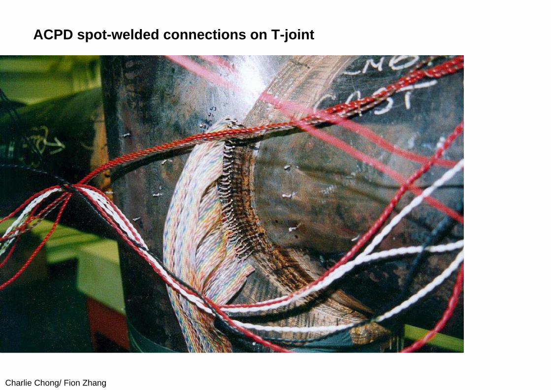
What can TSC offer?TSC can provide systems to carry out crack monitoring using either the a.c. potential drop (ACPD) technique, or the a.c. field measurement (ACFM) technique. Refer to other TSC literature for further information on these two techniques. Both systems use the Model U10 Crack Microgauge instrument and Flair software to provide crack size (length and depth) as a function of position on the test site (i.e. crack profile) and of time (i.e. a crack growth curve). Cable lengths between the test site and the instrument can be up to 20m.
Charlie Chong/ Fion Zhang
ACPD spot-welded connections on T-joint

Charlie Chong/ Fion Zhang
ACFM array on T-butt
Charlie Chong/ Fion Zhang
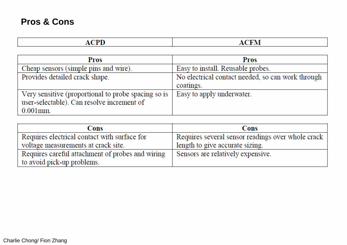
Pros & Cons
Charlie Chong/ Fion Zhang
By using permanently installed sensors, and ratios of two voltage measurements to compensate for drift in instrument settings or environmental effects, both techniques can give an accuracy in measurement of incremental growth of around 0.01mm or 0.1%. It should be noted that absolute accuracy of crack depth is lower than this because of variations in probe spacing, pick-p signals etc. Normal absolute accuracy of an isolated measurement on an existing crack is typically 10%. However, if it can be assumed that initial crack depth is zero (or if the depth of a pre-crack can be measured precisely), absolute accuracy can be as high as incremental accuracy.
Charlie Chong/ Fion Zhang
Examples of UsageCrack monitoring by ACPD has been used in laboratory situations for most standard fatigue test specimens (CT, tensile, 3-point bend etc.) as well as larger test pieces, such as tubular welded joints. These applications have included testing in corrosion cells containing sea water. Conventionally, these test use multiple spot-welded test points, but in the clean, dry conditions of a laboratory, it has also been possible to use sprung contact points driven across a flat sample by stepper motor. By using special materials in the construction of the contacts, housing and wiring, crack monitoring with both ACPD and ACFM has been carried out in hostile environments including high temperature (pipework at 600oC under lagging), and high radioactivity.
Charlie Chong/ Fion Zhang
Potential applications offshore include monitoring critical areas underwater on offshore structures, or monitoring on unmanned offshore installations. This would be done using ACFM sensor arrays to avoid problems of loss of contact, and would use waterproof instrumentation. Monitoring of underwater sites could be achieved either by fitting signal boosters to allow the voltages to be read by an instrument above water, or by developing an unconnected system which is activated and interrogated periodically (by diver or ROV) using wet-mateable power/comms connections (?).
Charlie Chong/ Fion Zhang
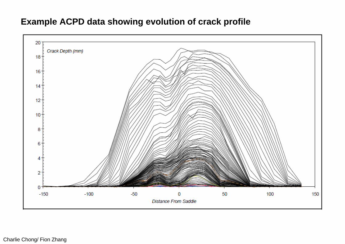
Example ACPD data showing evolution of crack profile
Charlie Chong/ Fion Zhang
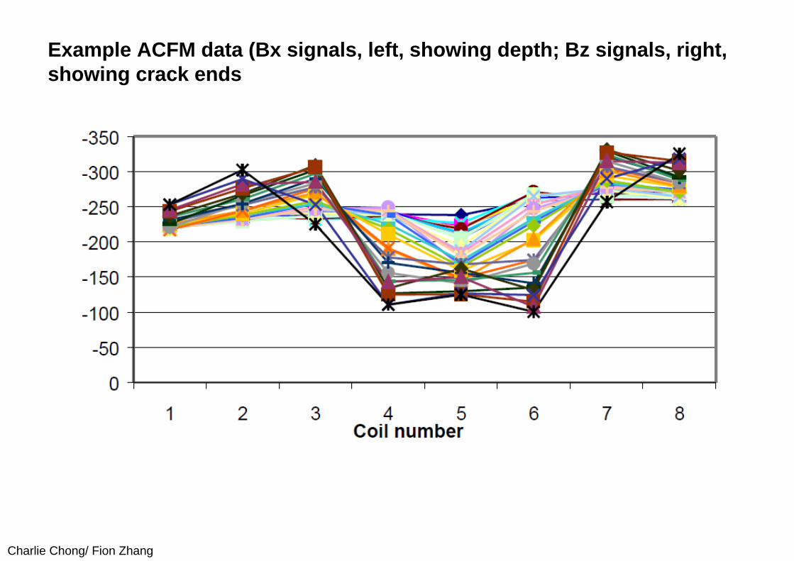
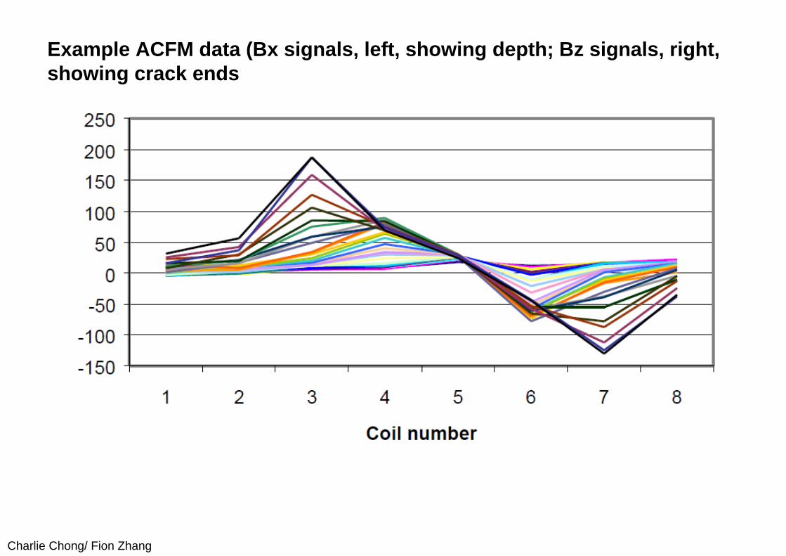
Example ACFM data (Bx signals, left, showing depth; Bz signals, right, showing crack ends
Charlie Chong/ Fion Zhang
Example ACFM data (Bx signals, left, showing depth; Bz signals, right, showing crack ends
Charlie Chong/ Fion Zhang
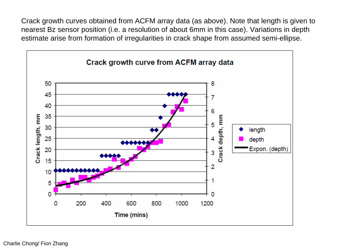
Crack growth curves obtained from ACFM array data (as above). Note that length is given to nearest Bz sensor position (i.e. a resolution of about 6mm in this case). Variations in depth estimate arise from formation of irregularities in crack shape from assumed semi-ellipse.
Charlie Chong/ Fion Zhang
Reading 5: Crack Monitoring using ACFM
AbstractKey input data for Structural Integrity Monitoring (SIM) calculations are the service stresses and the crack/defect size. To satisfy the second requirement the Alternating Current Field Measurement (ACFM) technique has been developed. Initially this was for the offshore oil and gas industry but it is now used very widely in other industries. ACFM allows one to detect and size surface cracks during both subsea and topside inspection. However a recent innovation for ACFM has been the introduction of array probes. Array probes have several sensors in one probe arranged in one or several rows thus allowing the collection of crack depth information from various sites along a crack in one placement of the probe.
The array probe is an area or strip inspection and hence can also be used for crack size monitoring if left in place on the structure. Array probes have now been used for both continuous monitoring and intermittent measurements and an example of these two modes of operation is given in this paper.
http://www.tscinspectionsystems.co.uk/pdfdocs/ApplicationCrackGrowthMonitoring.pdf
Charlie Chong/ Fion Zhang
Background to ACFM
ACFM is an electromagnetic technique for detecting and sizing surface breaking cracks. ACFM is an acronym for alternating current field measurement and was developed during the 1980’s from the A.C. potential drop (ACPD) technique.
The initial theoretical work was undertaken at University College London but since then the marketing of practical instruments and probes has been carried out by TSC Inspection Systems located in the UK.
Its conventional application is for the detection and characterization of fatigue cracks in and around welded joints but is increasingly used to detect a variety of surface breaking defects. Mathematical models of the field interaction with the cracks enable the crack length and depth to be predicted.
Keywords:Mathematical models of the field interaction with the cracks enable the crack length and depth to be predicted.
Charlie Chong/ Fion Zhang
Mathematical model
This mathematical model is based on a defect morphology that is semi-elliptical in shape, the most common shape in fatigue induced cracks. It should be noted that the crack model is not limited to a fixed aspect ratio but the largest depth that can be determined is usually half of the crack length measurement. ACFM has been approved by Lloyds, ABS, BV, DNV, andOCB Germanischer Lloyd for the inspection of offshore installations. ASTM has recently incorporated it as a Standard Practice for the examination of welds (E2261-03). ACFM is recognised as a technique by ASNT and a chapter devoted to ACFM is included in the Non-destructive Testing Handbook, third edition, volume 5: Electromagnetic Testing.
Charlie Chong/ Fion Zhang
Continuous Crack Monitoring
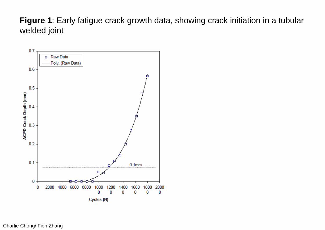
Many crack monitoring studies have been completed in the laboratory using ACPD (Alternating Current Potential Difference). These were research projects where it was necessary to monitor crack shape evolution in welded connections in order to confirm the results of fracture mechanics studies. ACPD requires electrical contact with the metal surface and hence the ACPD contacts were usually spot-welded to the test component at the weld toe.. The results from this work were of high quality and an example of early fatigue crack growth on a tubular welded T joint tested under variable amplitude corrosion fatigue [2] is shown in Figure 1. It can be seen that with ACPD it was possible to monitor early crack growth even with a connection spacing of 5 mm. This was because the crack aspect ratio was often large in this early period of crack growth. After the development of the non-contacting ACFM technique from ACPD it became possible to monitor cracks without the need to attach probes as the sensor spacing could be of the same order as the ACPD studies .
Charlie Chong/ Fion Zhang
Figure 1: Early fatigue crack growth data, showing crack initiation in a tubular welded joint
Charlie Chong/ Fion Zhang
In a more recent series of fatigue tests [3] this new approach has been demonstrated using array probes for monitoring. Thearray probes consisted of eight Bx and Bz coils arranged in a row at 10mm spacing. Four array probes were used to cover an area 160x20mm. The fatigue tests were conducted on a high strength steel (of the type proposed for use in jack ups), in four point bending at a frequency of 2Hz and a stress range of 200MPa. The specimen dimensions were 600 x 150 x 20mm and the weld had been ground to give a smooth finish.
Some detail of one of the tests is given here as an illustration of monitoring. The test occupied a total of 1.1 million cycles and the majority of the crack data occurred over the last night of the test. In this case the weld grinding had produced a long initiation period.
Charlie Chong/ Fion Zhang
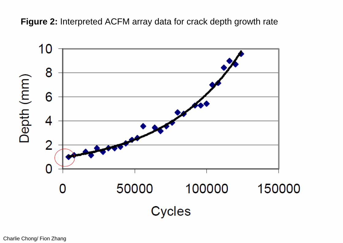
Figure 2 shows the interpreted ACFM array data for crack depth growth rate for the latter part of the test. The test ended in a fast fracture from a crack which appeared to be 10mm deep. It can be seen that the ACFM array probe showed a gradual increase in the crack growth rate right up to the final fracture. The final crack size was measured by visual inspection after the fracture event and found to be 10mm deep and 50mm long.
It can be seen the final prediction of crack size was correct i.e 10mm. However the aspect ratio was 5 to 1 (due to the absence of the weld toe stress concentration factor) and hence the early crack growth was not recorded until the crack was over 1mm deep. This problem would have occurred with ACPD as well. An alternative array system has recently been made and this utilises an array that can be periodically swept along the anticipated crack path by 10 or 15 mm. This adaptation should allow the detection and study of smaller cracks.
Charlie Chong/ Fion Zhang
Figure 2: Interpreted ACFM array data for crack depth growth rate
Charlie Chong/ Fion Zhang
Intermittent crack monitoring: Coke drumsIt is not always necessary to monitor continuously for SIM purposes. In some applications crack growth can be very slow. In such circumstances occasional intervention to obtain a periodic assessment of the condition is appropriate.
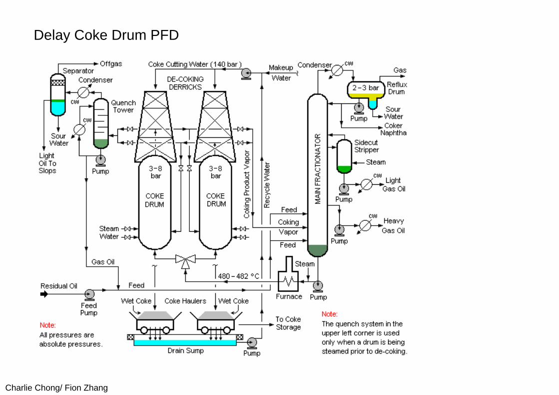
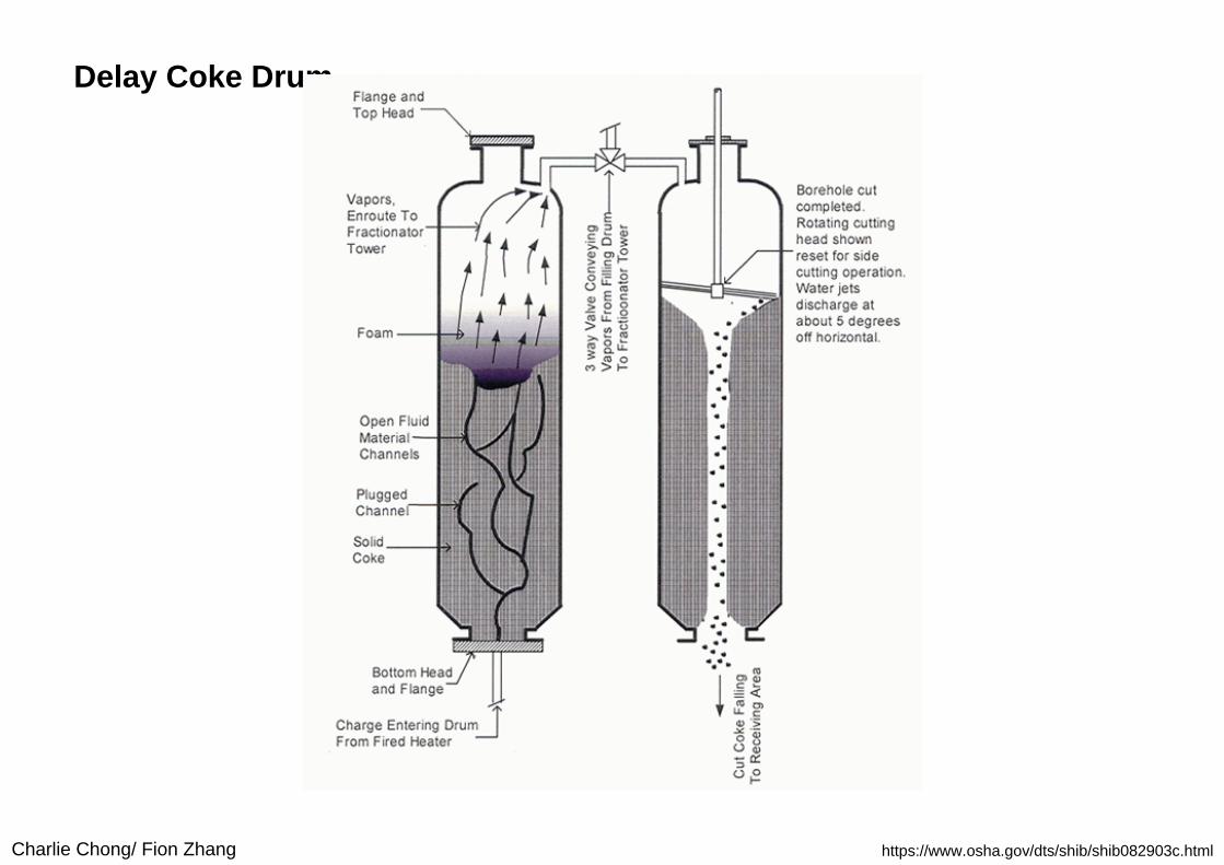
An example of this type is the delayed coke drum. Delayed coke drums are operated under severe conditions of cyclic heating and forced cooling that apply repetitive thermal stresses to the drum walls. It has long been recognized that the ultimate failure mechanism for coke drums is weld cracking due to low cycle fatigue caused by these thermal stresses. It is also known that coke drums distort and bulge in service and that these bulges can be used as pointers to potential weld failure areas. Key features of the technique which lends itself to internal inspection of coke drums include its suitability for remote, robotic deployment and the ability to work on relatively dirty surfaces.
Charlie Chong/ Fion Zhang
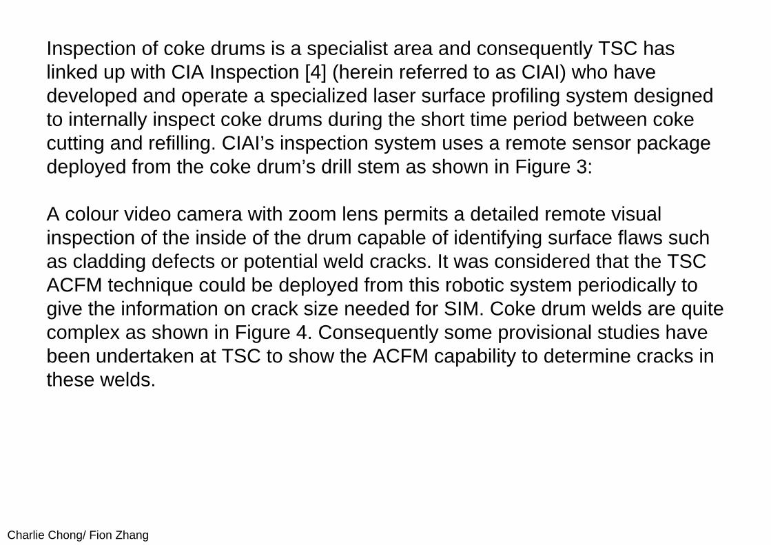
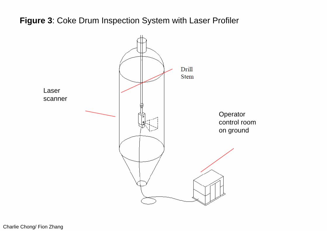
Inspection of coke drums is a specialist area and consequently TSC has linked up with CIA Inspection [4] (herein referred to as CIAI) who have developed and operate a specialized laser surface profiling system designed to internally inspect coke drums during the short time period between coke cutting and refilling. CIAI’s inspection system uses a remote sensor package deployed from the coke drum’s drill stem as shown in Figure 3:
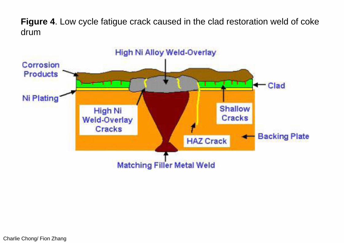
A colour video camera with zoom lens permits a detailed remote visual inspection of the inside of the drum capable of identifying surface flaws such as cladding defects or potential weld cracks. It was considered that the TSC ACFM technique could be deployed from this robotic system periodically to give the information on crack size needed for SIM. Coke drum welds are quite complex as shown in Figure 4. Consequently some provisional studies have been undertaken at TSC to show the ACFM capability to determine cracks in these welds.
Charlie Chong/ Fion Zhang
Figure 3: Coke Drum Inspection System with Laser Profiler
Laserscanner
Operatorcontrol roomon ground
Charlie Chong/ Fion Zhang
Figure 4. Low cycle fatigue crack caused in the clad restoration weld of coke drum
Charlie Chong/ Fion Zhang
Delay Coke Drum PFD
Charlie Chong/ Fion Zhang
Delay Coke Drum
https://www.osha.gov/dts/shib/shib082903c.html

Charlie C
hong/ Fion Zhang
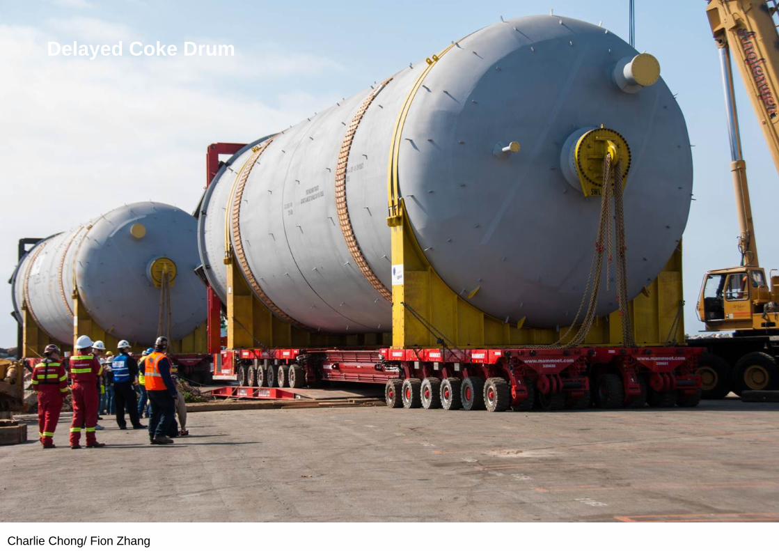
Delayed Coke Drum
Charlie Chong/ Fion Zhang
Delayed Coke Drum
Charlie Chong/ Fion Zhang
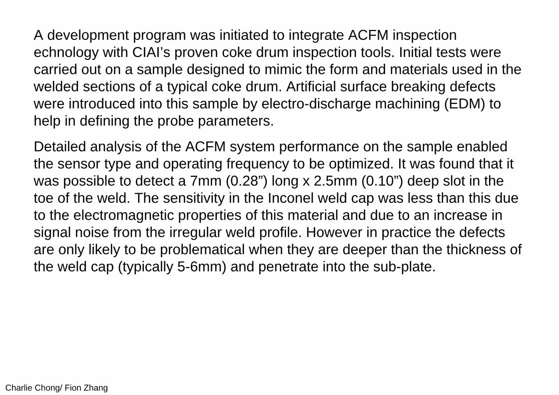
A development program was initiated to integrate ACFM inspectionechnology with CIAI’s proven coke drum inspection tools. Initial tests were carried out on a sample designed to mimic the form and materials used in the welded sections of a typical coke drum. Artificial surface breaking defects were introduced into this sample by electro-discharge machining (EDM) to help in defining the probe parameters.
Detailed analysis of the ACFM system performance on the sample enabled the sensor type and operating frequency to be optimized. It was found that it was possible to detect a 7mm (0.28”) long x 2.5mm (0.10”) deep slot in the toe of the weld. The sensitivity in the Inconel weld cap was less than this due to the electromagnetic properties of this material and due to an increase in signal noise from the irregular weld profile. However in practice the defects are only likely to be problematical when they are deeper than the thickness of the weld cap (typically 5-6mm) and penetrate into the sub-plate.

Charlie Chong/ Fion Zhang
The system uses a custom designed ACFM sensor head composed of an rray of individual sensors incorporated into an integral package. The size and spacing of the sensors are configured depending on the target defect size and other operating factors. The requirement is to be able to scan the weld, both toes and a little into the HAZ with one pass of the probe. This is achieved by using 16 sensor pairs, which cover a width of approximately 114mm (4.5"). A typical ACFM result is shown in Figure 5.
With this newly developed remote crack detection system, management now has the capability to assess the significance of the surface indications without scaffolding, insulation removal or vessel entry. It allows the number and location of relevant indications in the drum to be measured periodically. The results of these investigations would confirm if visual indication are really cracks and it would also characterize the crack so that management could make a decision on the urgency to make a repair.
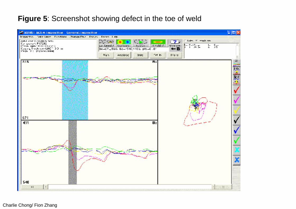
Charlie Chong/ Fion Zhang
Figure 5: Screenshot showing defect in the toe of weld
Charlie Chong/ Fion Zhang
SUMMARYMonitoring of cracks continuously and intermittently allows the continuing assessment for structural integrity. A side product of this activity is that often the quality of crack information is superior to that obtained in a single intervention. This high quality data on crack size allows the facility owner the opportunity to schedule repairs and to maximize the use of equipment. The TSC CIAI development is an example of this new approach and this will be operational in 2006.
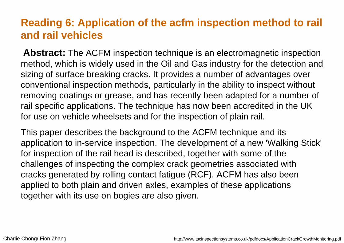
Charlie Chong/ Fion Zhang
Reading 6: Application of the acfm inspection method to rail and rail vehiclesAbstract: The ACFM inspection technique is an electromagnetic inspection method, which is widely used in the Oil and Gas industry for the detection and sizing of surface breaking cracks. It provides a number of advantages over conventional inspection methods, particularly in the ability to inspect without removing coatings or grease, and has recently been adapted for a number of rail specific applications. The technique has now been accredited in the UK for use on vehicle wheelsets and for the inspection of plain rail.
This paper describes the background to the ACFM technique and its application to in-service inspection. The development of a new 'Walking Stick' for inspection of the rail head is described, together with some of the challenges of inspecting the complex crack geometries associated with cracks generated by rolling contact fatigue (RCF). ACFM has also been applied to both plain and driven axles, examples of these applications together with its use on bogies are also given.
http://www.tscinspectionsystems.co.uk/pdfdocs/ApplicationCrackGrowthMonitoring.pdf
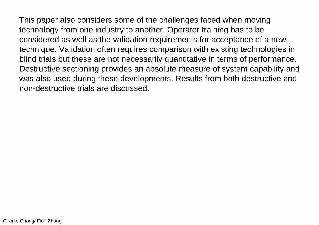
Charlie Chong/ Fion Zhang
This paper also considers some of the challenges faced when moving technology from one industry to another. Operator training has to be considered as well as the validation requirements for acceptance of a new technique. Validation often requires comparison with existing technologies in blind trials but these are not necessarily quantitative in terms of performance. Destructive sectioning provides an absolute measure of system capability and was also used during these developments. Results from both destructive and non-destructive trials are discussed.
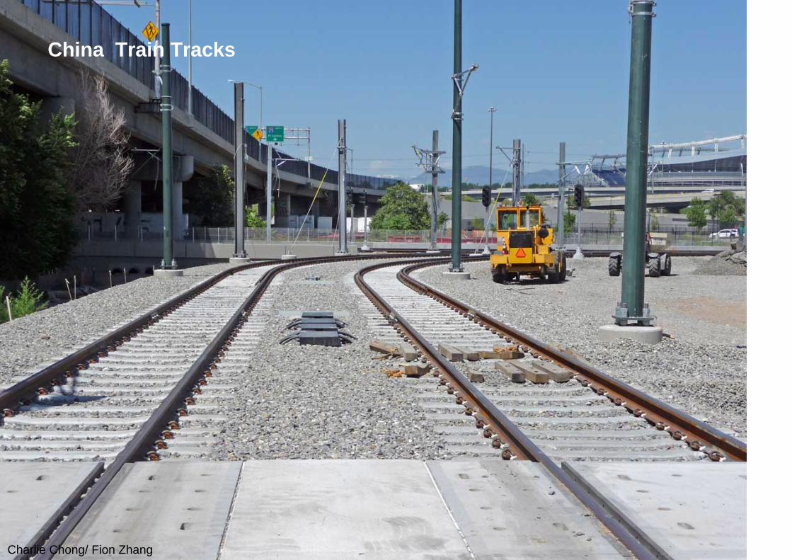
Charlie Chong/ Fion Zhang
China Train Tracks
Charlie Chong/ Fion Zhang
China High Speed Train
Charlie Chong/ Fion Zhang
China High Speed Train
Charlie Chong/ Fion Zhang
China Train Tracks
Charlie Chong/ Fion Zhang
Train Tracks
Charlie Chong/ Fion Zhang
Train Tracks
Charlie Chong/ Fion Zhang
Train Tracks
Charlie Chong/ Fion Zhang
Train Tracks
Charlie Chong/ Fion Zhang
Train Tracks
Charlie Chong/ Fion Zhang
Train Tracks
Charlie Chong/ Fion Zhang
Introduction: The Alternating Current Field Measurement (ACFM) technique is anelectromagnetic inspection method capable of surface crack detection and sizing. The technique does not require coating removal and was originally developed in the late 1980s for use in the Oil Industry, where there was a requirement for improving the reliability of subsea inspection. The first application of ACFM in the rail industry was for the inspection of axles. This came about from a review of available crack detection methods conducted by the Engineering Link following a fatal accident involving the failure of an axle. This review, which looked beyond those methods traditionally used in the rail industry, was followed up by a series of blind trials1 in which the ACFM technique was found to outperform conventional Magnetic Particle Inspection (MPI) and an advanced eddy current method.
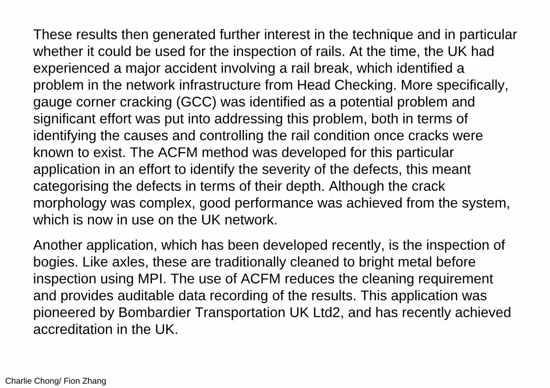
Charlie Chong/ Fion Zhang
These results then generated further interest in the technique and in particular whether it could be used for the inspection of rails. At the time, the UK had experienced a major accident involving a rail break, which identified a problem in the network infrastructure from Head Checking. More specifically, gauge corner cracking (GCC) was identified as a potential problem and significant effort was put into addressing this problem, both in terms of identifying the causes and controlling the rail condition once cracks were known to exist. The ACFM method was developed for this particular application in an effort to identify the severity of the defects, this meant categorising the defects in terms of their depth. Although the crack morphology was complex, good performance was achieved from the system, which is now in use on the UK network.
Another application, which has been developed recently, is the inspection of bogies. Like axles, these are traditionally cleaned to bright metal before inspection using MPI. The use of ACFM reduces the cleaning requirement and provides auditable data recording of the results. This application was pioneered by Bombardier Transportation UK Ltd2, and has recently achieved accreditation in the UK.
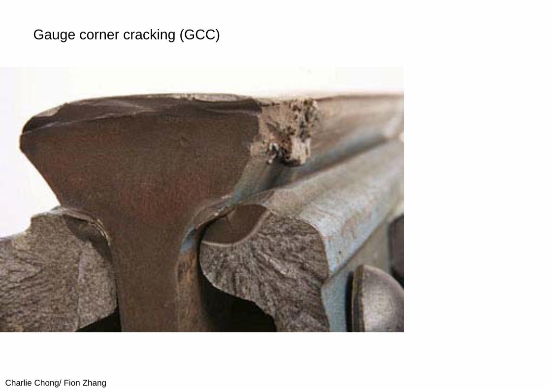
Charlie Chong/ Fion Zhang
Gauge corner cracking (GCC)
Charlie Chong/ Fion Zhang
The ACFM Method: The Alternating Current Field Measurement (ACFM) technique is an electromagnetic technique capable of both detecting and sizing (length and depth) surface breaking cracks in metals. The basis of the technique is that an alternating current can be induced to flow in a thin skin near the surface of any conductor. By introducing a remote uniform current into an area of the component under test, when there are no defects present the electrical current will be undisturbed. If a crack is present the uniform current is disturbed and the current flows around the ends and down the faces of the crack. Because the current is an alternating current (AC) it flows in a thin skin close to the surface and is unaffected by the overall geometry of the component.
Keywords:AC Current can be induced to flow in a thin skin near the surface of any conductor.
Charlie Chong/ Fion Zhang
Associated with the current flowing in the surface is a magnetic field above the surface which, like the current in the surface, will be disturbed in the presence of a defect. An important factor of the ACFM technique is its capability to relate measurements of the magnetic field disturbance to the size of defect that caused that disturbance. The breakthrough came from a combination of studies at University College London, which provided mathematical modelling of the magnetic field rather than electrical fields, and advances in electronics and sensing technology.
Charlie Chong/ Fion Zhang
Although the magnetic field above the surface is a complex 3D field, it is possible, by choosing suitable orthogonal axes, to measure components of the field that are indicative of the nature of the disturbance and which can be related to the physical properties of any cracks present. Figure 1 presents a plan view of a surface breaking crack where a uniform ac current is flowing. The field component denoted Bz in figure 1 responds to the poles generated as the current flows around the ends of the crack introducing current rotations in the plane of the component. These responses are principally at the crack ends and are indicative of crack length. The field component denoted Bx responds to the reduction in current surface density as the current flows down the crack and is indicative of the depth of the defects. Generally the current is introduced perpendicular to the expected direction of cracking so for a shaft or axle subjected to fatigue, the current would be introduced in an axial direction to be disturbed by cracks in a circumferential direction.
Charlie Chong/ Fion Zhang
In practice special probes have been developed which contain a remote field induction system, for introducing the field into the component, together with special combined magnetic field sensors that allow accurate measurement of the components of the magnetic field at the same point in space. The probe requires no electrical contact with the component and can therefore be applied without the removal of surface coatings or grime.
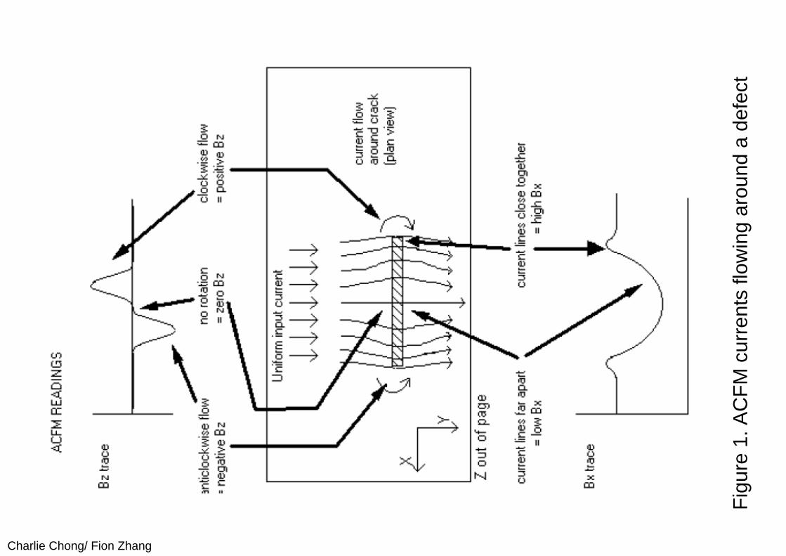
Charlie Chong/ Fion Zhang
Figu
re 1
. AC
FM c
urre
nts
flow
ing
arou
nd a
def
ect
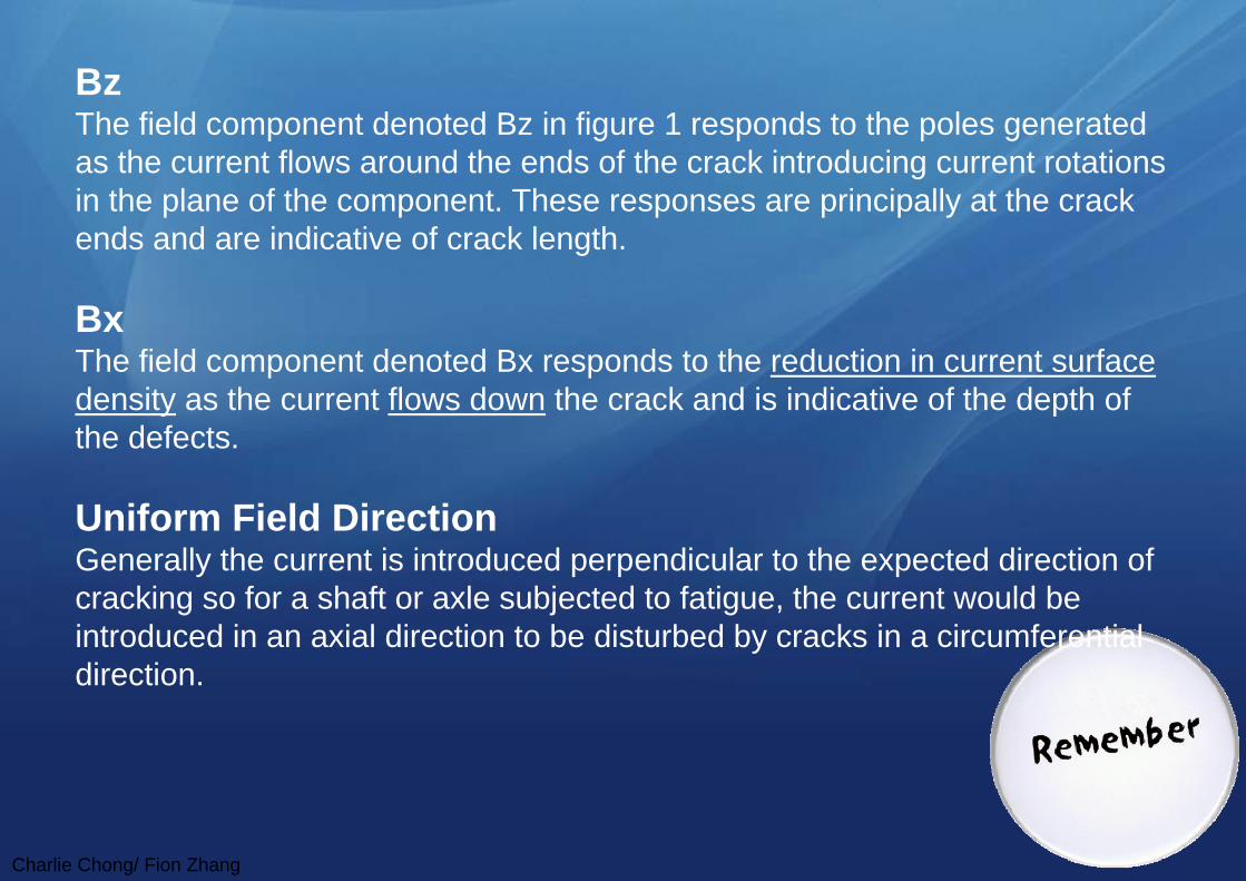
Charlie Chong/ Fion Zhang
BzThe field component denoted Bz in figure 1 responds to the poles generated as the current flows around the ends of the crack introducing current rotations in the plane of the component. These responses are principally at the crack ends and are indicative of crack length.
BxThe field component denoted Bx responds to the reduction in current surface density as the current flows down the crack and is indicative of the depth of the defects.
Uniform Field DirectionGenerally the current is introduced perpendicular to the expected direction of cracking so for a shaft or axle subjected to fatigue, the current would be introduced in an axial direction to be disturbed by cracks in a circumferential direction.
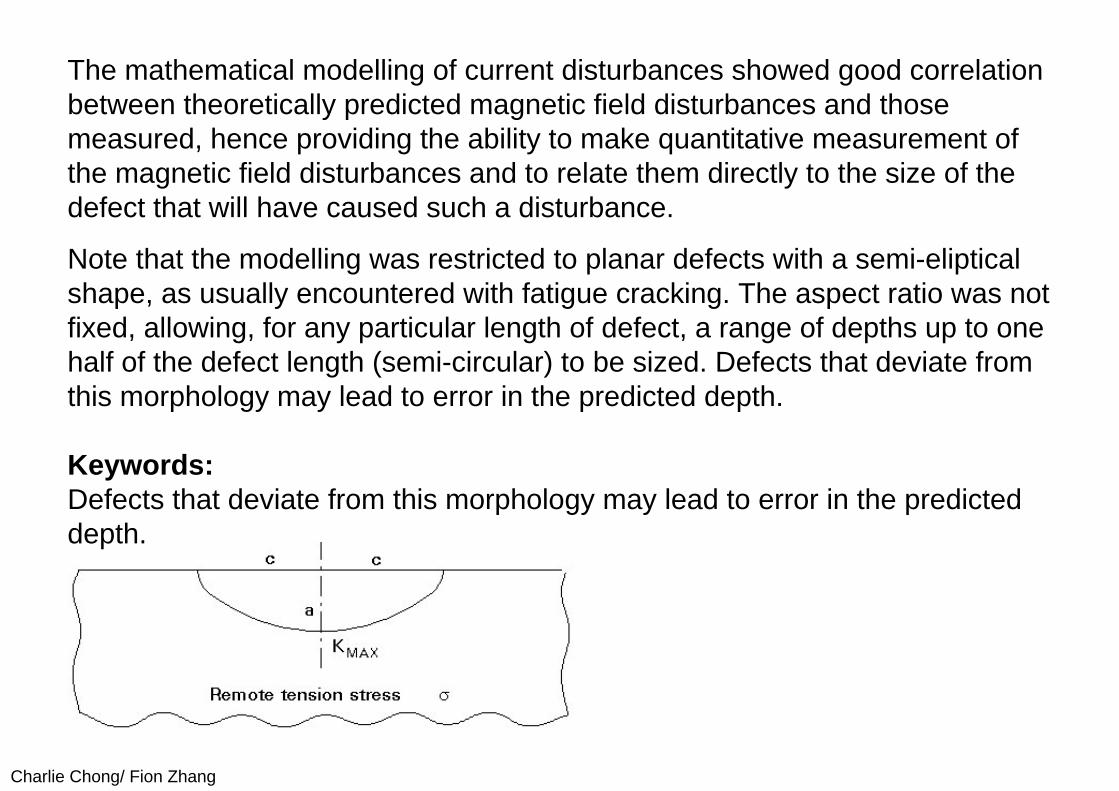
Charlie Chong/ Fion Zhang
The mathematical modelling of current disturbances showed good correlation between theoretically predicted magnetic field disturbances and those measured, hence providing the ability to make quantitative measurement of the magnetic field disturbances and to relate them directly to the size of the defect that will have caused such a disturbance.
Note that the modelling was restricted to planar defects with a semi-elipticalshape, as usually encountered with fatigue cracking. The aspect ratio was not fixed, allowing, for any particular length of defect, a range of depths up to one half of the defect length (semi-circular) to be sized. Defects that deviate from this morphology may lead to error in the predicted depth.
Keywords:Defects that deviate from this morphology may lead to error in the predicted depth.
Charlie Chong/ Fion Zhang
From a practical standpoint, the technique can be applied using a single probe that can be manually moved along a component. Experience showed that with earlier electromagnetic inspection systems, for example eddy current devices, there were a number of drawbacks when used in practical situations.
Many of these arose from signals from features other than cracks, leading to difficult interpretation of the signals. For example, even small amounts of probe lift off from the surface can cause large changes in a standard eddy current response.
The ACFM technique has virtually eliminated this and other related problems by use of the uniform field together with careful probe and electronics design, but in particular by utilising special displays of the data. A standard PC is used to control the equipment and display results. ACFM is unique in the way data is displayed.
Charlie Chong/ Fion Zhang
How ACFM overcomes lift-off problems?
The ACFM technique has virtually eliminated this and other related problems by use of the:
uniform field together with careful probe and electronics design, but in particular by utilizing special displays of the data.
A standard PC is used to control the equipment and display results. ACFM is unique in the way data is displayed.
Charlie Chong/ Fion Zhang
The plot on the left of figure 2 shows typical raw data from the crack end and crack depth sensors collected from a manually deployed probe. The right hand section of figure 2 shows this presented as a butterfly plot. In the presence of a defect, the butterfly loop is drawn in the screen and for manual operation the operator looks for this distinctive shape to decide whether a crack is present or not. Having detected a defect, the data can be subsequently interrogated to determine the depth of the crack without calibration. All data is stored by the system and is available for subsequent review and analysis. This is particularly useful for audit purposes and for reporting.
Because ACFM uses a remote uniform field, it is possible to make a number of field measurements at different positions in the same field. This concept is used for both axles and rail inspection by producing a probe, profiled to the component and containing multiple field sensors. This 1D array of sensors can then be swept along or around surface to provide inspection of the scanned area.
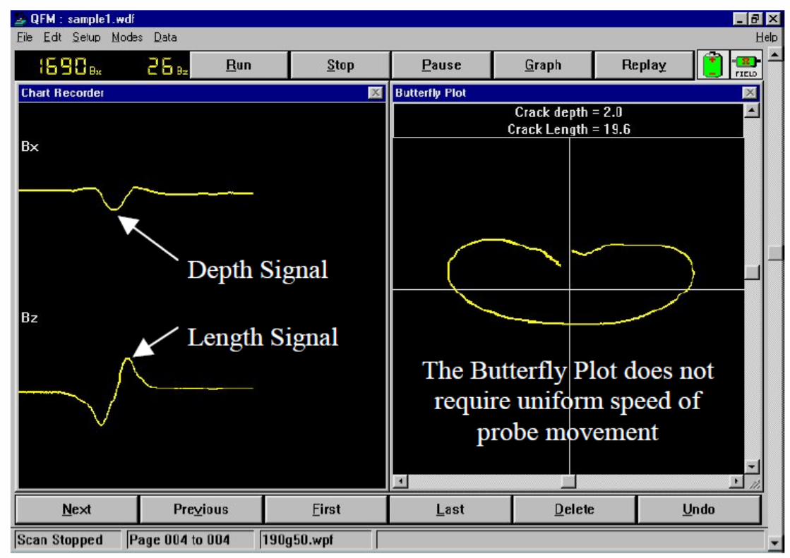
Charlie Chong/ Fion Zhang
1111
Charlie Chong/ Fion Zhang
Application of ACFM to Axles:
Following its successful performance in the Engineering Link axle trials, ACFM has been gradually introduced for the surface inspection of railway axles as a replacement for MPI. Due to its ability to operate through coatings, ACFM inspection can be conducted on painted axles without the need to strip and re-paint. This can provide a major saving in time and costs as well as aiding in corrosion integrity by not disturbing the original coating. Because the ACFM technique records all inspection data, there is a permanent record of the inspection available should an axle fail in service.
Charlie Chong/ Fion Zhang
Axles can be inspected either on or off the vehicle. In the latter case, it is usually most convenient to mount the axle in an engineering lathe and to mount the ACFM probe onto a tool post that can be scanned along the length of the axle while it is rotated. In this way, the whole axle body can be inspected in a continuous helical scan.
If the axle is to be inspected on the vehicle then it is usual to use an array probe. These are larger probes which contain multiple sensors and can inspect a much wider area that standard probes. Each of the sensors is sampled as the probe is moved and an integral encoder logs the distance travelled into the software. The axle is inspected in overlapping bands as the probe is scanned around the axle.
Charlie Chong/ Fion Zhang
the section of axle under the Earth Return Brush (ERB) on an in-service power axle. Access to the area could be achieved by removing the brush and its holder leaving a small circular aperture approximately 90mm (3.5inches) in diameter and 50mm (2.0") deep. MPI was not considered suitable due to the restricted access and the problem with the use of contaminating fluids on an in-service box. Due to axle geometry, Ultrasonic inspection was also not possible.
A custom ACFM array probe was designed and manufactured to fit through the access hole and inspect the axle under the brush with the axle in place on the train. Figure 3 shows the probe which contains 8 sensors covering an area of 70mm (2.8inches).
Deployment was carried out by jacking the appropriate bogie to raise the wheels off the rails, then rotating the wheel while data was collected. In this way, the entire inspection site could be inspected with just one rotation of the axle.
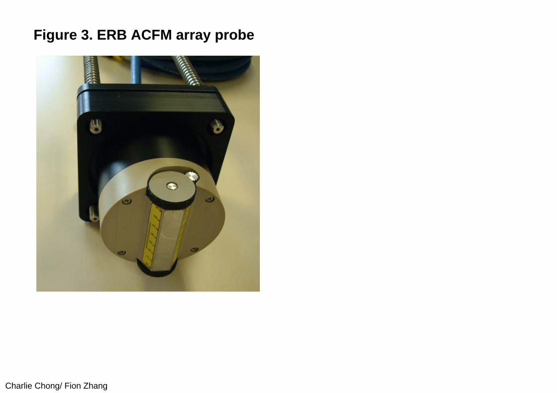
Charlie Chong/ Fion Zhang
Figure 3. ERB ACFM array probe
Charlie Chong/ Fion Zhang
Application of ACFM to rails:
As described above, the ACFM method was originally developed for manual inspection of welds. Here the requirements are very specific, generally the inspection area is a narrow strip near the weld toes and, because the inspections are carried out manually, the scan speed can be relatively slow, perhaps 10mm per second for short periods. The requirement for rail inspection was very different. There was a requirement to inspect a wider area, covering the gauge face, gauge corner and across the head towards tofield side. The speed of inspection needed to be as high a possible, in order to achieve acceptable throughput. It was also desirable to have automated interpretation of the results.
Charlie Chong/ Fion Zhang
Another major challenge was in the crack morphology. Typically GCC comprises multiple, closely spaced cracks at a large angle to the running direction. The cracks are often inclined to the surface, penetrating initially at an angle of approximately 30 degrees until they break through the compressive layer, about 5mm (0.2 inch) below the surface, when the angle increases to approximately 60 degrees.
The ultrasonic testing, that was conventionally being carried out, suffered from "crack shielding" whereby shallower defects could mask deeper defects and thereby undersize the greatest defect depth. Shallow cracking was also difficult for ultrasonics to identify and categorise. There is a poor correlation between crack surface length and penetration depth of the cracks and even short cracks can be deep.
However, due to the limitations of the then available techniques, the UK inspection standards dictated that GCC should be classified according to the greatest surface length rather than the depth – which is the more crucial in engineering terms.
Charlie Chong/ Fion Zhang
Coverage of the rail head was achieved by use of a sensor array, shaped to the head of the rail. In fact the probe was designed to take the shape of a wheel in order to optimise the location of the probe even on worn rail. The inspection across the rail head is carried out by sequentially scanning across the group of sensors. By doing this, a continuous scan of the rail head is achieved as the probe is pushed along the rail.
Speed was initially limited by the sampling rates achievable for a 5kHz input signal. For this application, this was increased to 50kHz and scanning speeds of 2-3km (1.3-1.9 miles) per hour have been achieved. It must be recognisedthat this is a quantitative inspection method and that sufficient data must be collected to not only detect, but also determine the severity of the cracking.
Charlie Chong/ Fion Zhang
The system has been packaged into a pedestrian 'Walking Stick' (figure 4) which is totally self contained and capable of operating for at least 8 hours from its own power source. The walking stick display is a ruggedised PC which controls the system and displays analysed data in a readily useable form for the operator. Very little operator interpretation is required. The ACFM method relies on predication of AC current flows on the surface of a component and the modelling has focussed on the planar semi elliptical cracks, typical of fatigue damage. The sizing models therefore didn't apply to the complex crack shapes synonymous with GCC.
Charlie Chong/ Fion Zhang
In order to provide real time crack sizing it was necessary to consider the mathematical modelling and its relevance to the GCC crack form. It was decided that the existing models would be used as a starting point and that empirical correction factors would be applied to take account of the crack type.
This obviously required a large amount of data on crack growth behaviour and that is difficult to achieve with any existing non-destructive testing methods. For this reason, it was decided to embark on a programme of destructive testing, which could be used to characterise the crack shape and at the same time to validate the results of blind trials using the ACFM method.
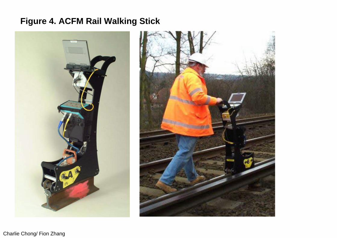
Charlie Chong/ Fion Zhang
Figure 4. ACFM Rail Walking Stick
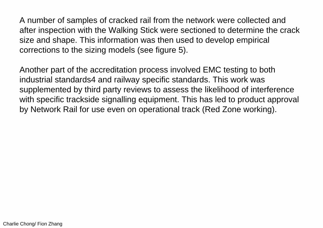
Charlie Chong/ Fion Zhang
A number of samples of cracked rail from the network were collected and after inspection with the Walking Stick were sectioned to determine the crack size and shape. This information was then used to develop empirical corrections to the sizing models (see figure 5).
Another part of the accreditation process involved EMC testing to both industrial standards4 and railway specific standards. This work was supplemented by third party reviews to assess the likelihood of interference with specific trackside signalling equipment. This has led to product approval by Network Rail for use even on operational track (Red Zone working).
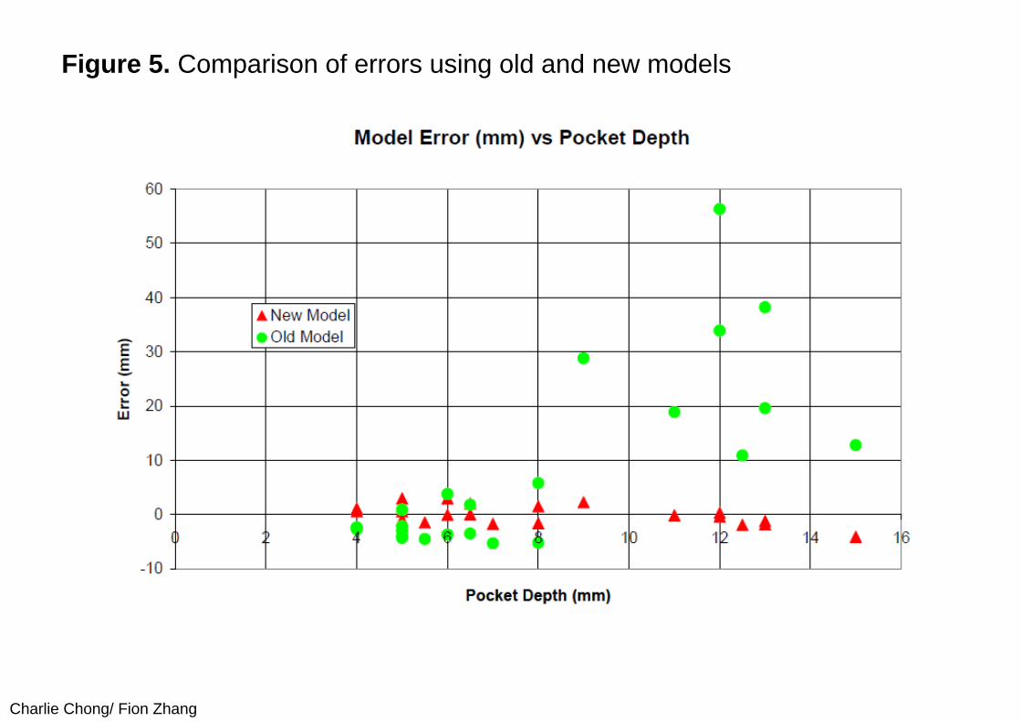
Charlie Chong/ Fion Zhang
Figure 5. Comparison of errors using old and new models
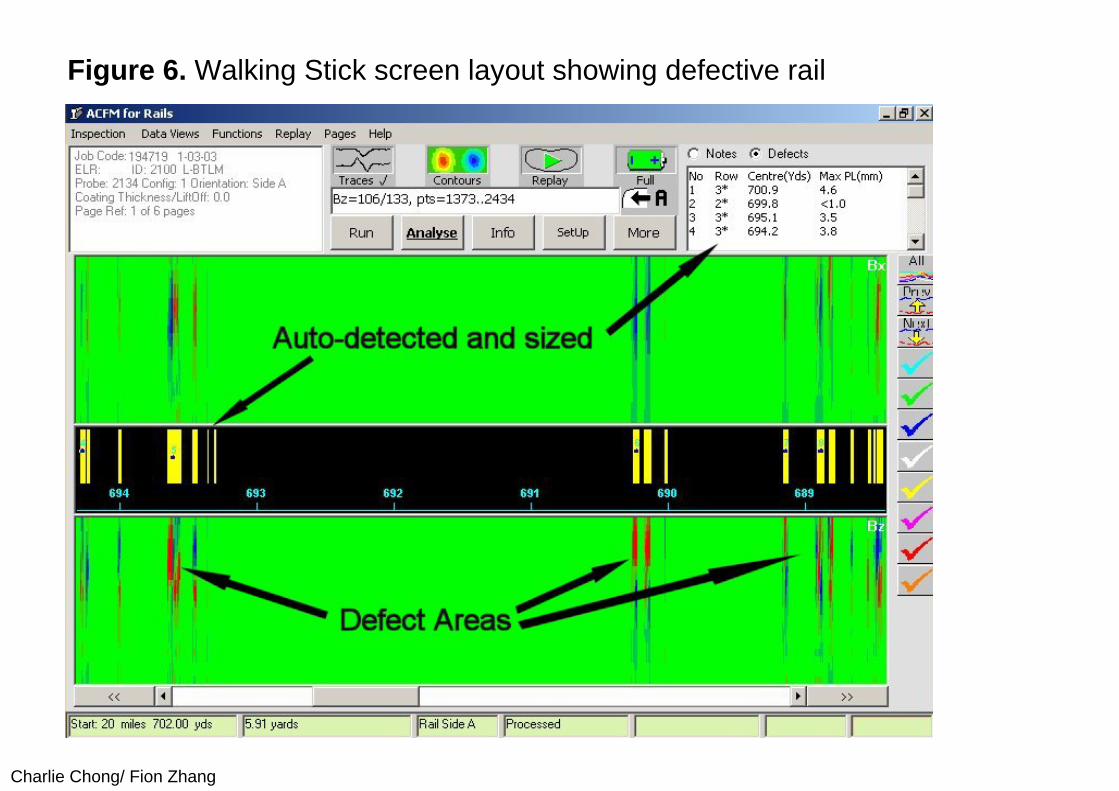
Charlie Chong/ Fion Zhang
Figure 6. Walking Stick screen layout showing defective rail
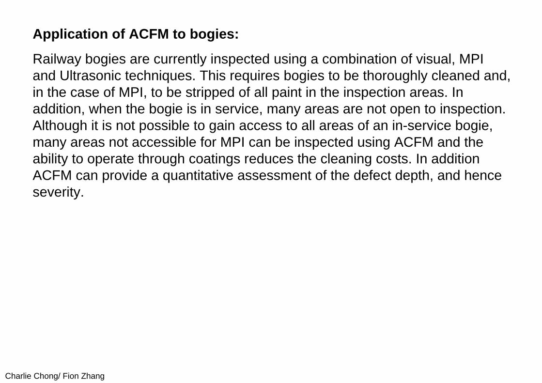
Charlie Chong/ Fion Zhang
Application of ACFM to bogies:
Railway bogies are currently inspected using a combination of visual, MPI and Ultrasonic techniques. This requires bogies to be thoroughly cleaned and, in the case of MPI, to be stripped of all paint in the inspection areas. In addition, when the bogie is in service, many areas are not open to inspection. Although it is not possible to gain access to all areas of an in-service bogie, many areas not accessible for MPI can be inspected using ACFM and the ability to operate through coatings reduces the cleaning costs. In addition ACFM can provide a quantitative assessment of the defect depth, and hence severity.
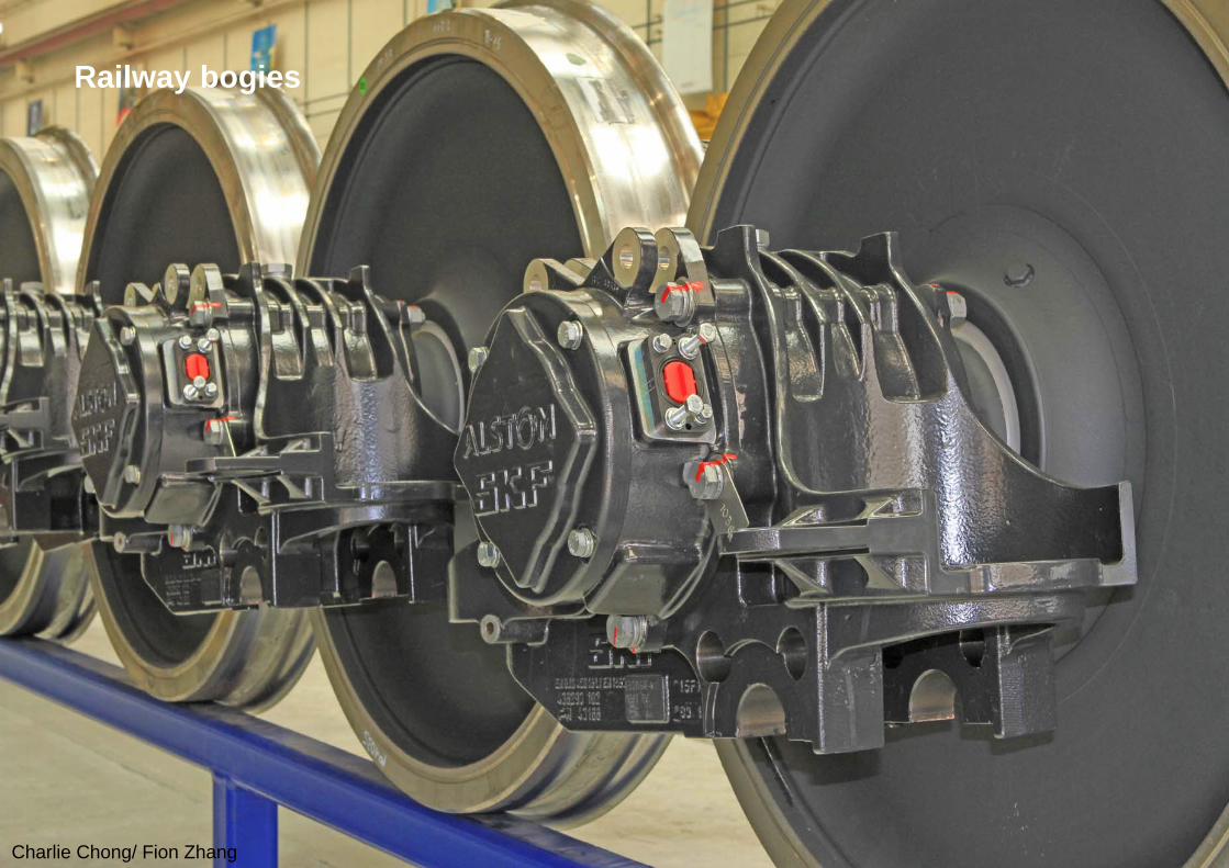
Charlie Chong/ Fion Zhang
Railway bogies
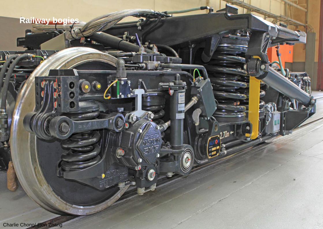
Charlie Chong/ Fion Zhang
Railway bogies
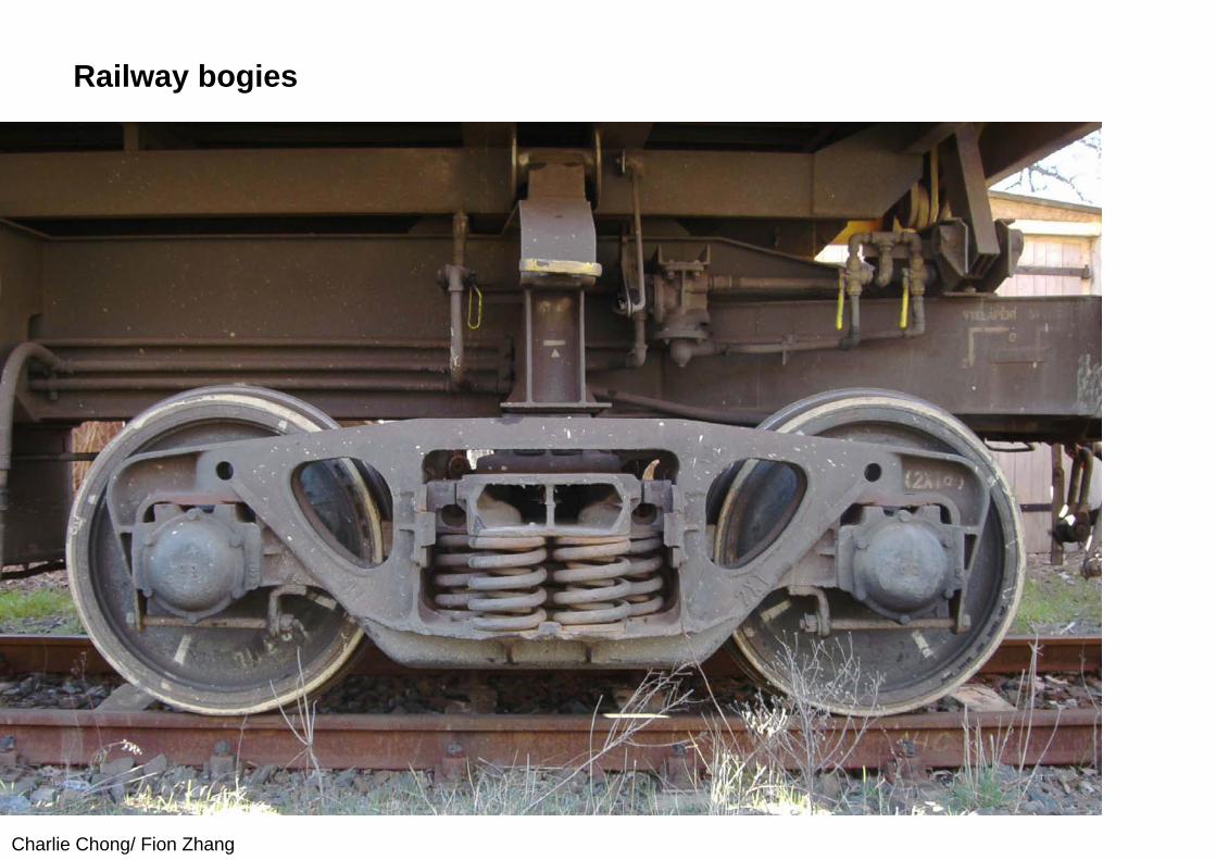
Charlie Chong/ Fion Zhang
Railway bogies
Charlie Chong/ Fion Zhang
Bombardier Transportation, UK recognised the potential for using ACFM to inspect bogies both at overhaul and in-service and launched a program to introduce ACFM into this sector of the rail industry. TSC developed equipment (figure 7) and probes to meet their target defect size of 5mm long x 0.5mm deep and to simplify inspection for the operator. Automated defect detection and sizing was introduced along with other operator aids to simplify and speed up the inspections. In order to provide an auditable and comprehensive report format for end clients, a semi-automated summary report scheme was introduced which could combine the results from all inspections on a particular bogie.
Charlie Chong/ Fion Zhang
To evaluate the performance of the technique and to certify its use for this application, Bombardier Transportation's Conformance Certification Body (CCB) and Vehicle Acceptance Body (VAB) conducted an extensive and detailed study. This study involved a literature search on all past papers, applications and performance reports, a full risk assessment, selective laboratory experiments and field trials. This culminated in a qualification dossier7 which was endorsed by The Engineering Link and The Welding Institute.
One initial application was the inspection of a UK type 91 bogie which had a previously inaccessible weld on the inside of a box section. Access was at arm's length through a small hole in the section enabling a probe to be deployed along the weld toes.
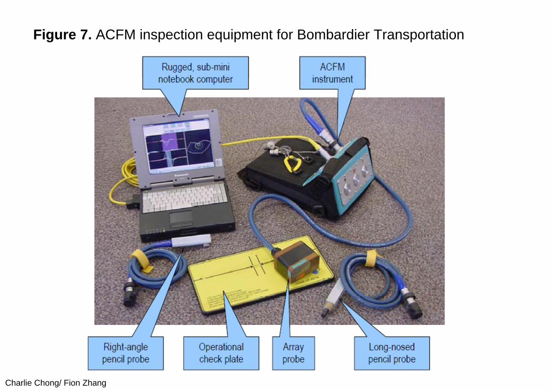
Charlie Chong/ Fion Zhang
Figure 7. ACFM inspection equipment for Bombardier Transportation
Charlie Chong/ Fion Zhang
Training: As with any inspection method, it necessary to ensure that operatives are properly trained and certified to operate the equipment. Special training courses have been developed together with operator certification, compliant with EN473. These have been developed for both Axle Inspection and Rail Inspection under the CSWIP certification Scheme8.
Conclusions: Introducing new inspection techniques into the rail industry is a challenge that involves many aspects of accreditation and approvals. It is also necessary to consider the skills level of operators and training requirements specific to that industry. This paper has shown how inspection technology originally developed for the Oil and gas Industry has met these challenges and been accepted for a number of different applications within the UK.

Charlie Chong/ Fion Zhang
TheThe Reading Magic

Charlie Chong/ Fion Zhang
The Reading Magic

Charlie Chong/ Fion Zhang

Charlie Chong/ Fion Zhang
ass