Embed Size (px)
Citation preview
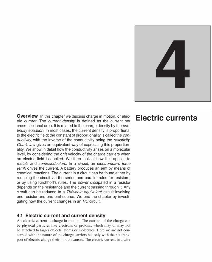
4Electric currentsOverview In this chapter we discuss charge in motion, or elec-
tric current. The current density is defined as the current percross-sectional area. It is related to the charge density by the con-tinuity equation. In most cases, the current density is proportionalto the electric field; the constant of proportionality is called the con-ductivity, with the inverse of the conductivity being the resistivity.Ohm’s law gives an equivalent way of expressing this proportion-ality. We show in detail how the conductivity arises on a molecularlevel, by considering the drift velocity of the charge carriers whenan electric field is applied. We then look at how this applies tometals and semiconductors. In a circuit, an electromotive force(emf) drives the current. A battery produces an emf by means ofchemical reactions. The current in a circuit can be found either byreducing the circuit via the series and parallel rules for resistors,or by using Kirchhoff’s rules. The power dissipated in a resistordepends on the resistance and the current passing through it. Anycircuit can be reduced to a Thévenin equivalent circuit involvingone resistor and one emf source. We end the chapter by investi-gating how the current changes in an RC circuit.
4.1 Electric current and current densityAn electric current is charge in motion. The carriers of the charge canbe physical particles like electrons or protons, which may or may notbe attached to larger objects, atoms or molecules. Here we are not con-cerned with the nature of the charge carriers but only with the net trans-port of electric charge their motion causes. The electric current in a wire
178 Electric currents
is the amount of charge passing a fixed mark on the wire in unit time.The SI unit of current is the coulomb/second, which is called an ampere(amp, or A):
1 ampere = 1coulombsecond
. (4.1)(a)
u
u
uu
u
a
q
q
q
(b)
u Δ t cosq
u Δ t
u
q
(b)
Δ tu Δ
qa
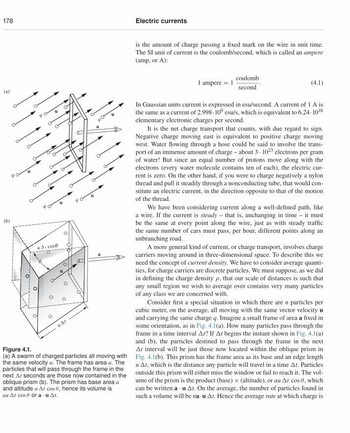
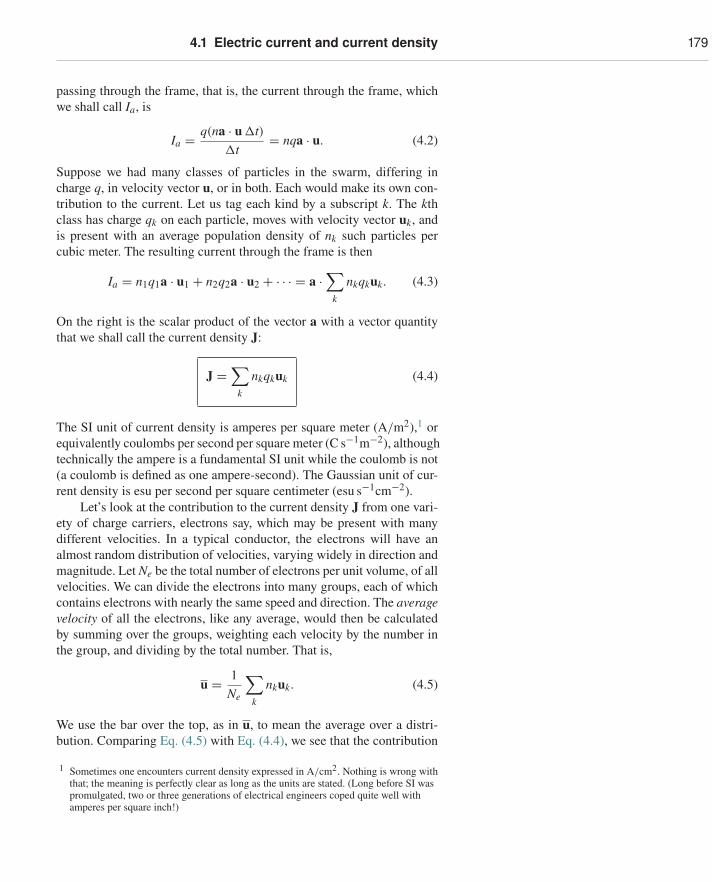
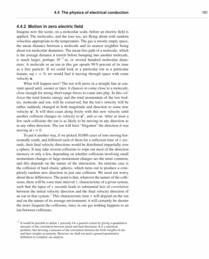
Figure 4.1.(a) A swarm of charged particles all moving withthe same velocity u. The frame has area a. Theparticles that will pass through the frame in thenext �t seconds are those now contained in theoblique prism (b). The prism has base area aand altitude u �t cos θ , hence its volume isau �t cos θ or a · u �t.
In Gaussian units current is expressed in esu/second. A current of 1 A isthe same as a current of 2.998·109 esu/s, which is equivalent to 6.24·1018
elementary electronic charges per second.It is the net charge transport that counts, with due regard to sign.
Negative charge moving east is equivalent to positive charge movingwest. Water flowing through a hose could be said to involve the trans-port of an immense amount of charge – about 3 · 1023 electrons per gramof water! But since an equal number of protons move along with theelectrons (every water molecule contains ten of each), the electric cur-rent is zero. On the other hand, if you were to charge negatively a nylonthread and pull it steadily through a nonconducting tube, that would con-stitute an electric current, in the direction opposite to that of the motionof the thread.
We have been considering current along a well-defined path, likea wire. If the current is steady – that is, unchanging in time – it mustbe the same at every point along the wire, just as with steady trafficthe same number of cars must pass, per hour, different points along anunbranching road.
A more general kind of current, or charge transport, involves chargecarriers moving around in three-dimensional space. To describe this weneed the concept of current density. We have to consider average quanti-ties, for charge carriers are discrete particles. We must suppose, as we didin defining the charge density ρ, that our scale of distances is such thatany small region we wish to average over contains very many particlesof any class we are concerned with.
Consider first a special situation in which there are n particles percubic meter, on the average, all moving with the same vector velocity uand carrying the same charge q. Imagine a small frame of area a fixed insome orientation, as in Fig. 4.1(a). How many particles pass through theframe in a time interval �t? If �t begins the instant shown in Fig. 4.1(a)and (b), the particles destined to pass through the frame in the next�t interval will be just those now located within the oblique prism inFig. 4.1(b). This prism has the frame area as its base and an edge lengthu �t, which is the distance any particle will travel in a time �t. Particlesoutside this prism will either miss the window or fail to reach it. The vol-ume of the prism is the product (base) × (altitude), or au �t cos θ , whichcan be written a · u �t. On the average, the number of particles found insuch a volume will be na·u �t. Hence the average rate at which charge is
4.1 Electric current and current density 179
passing through the frame, that is, the current through the frame, whichwe shall call Ia, is
Ia = q(na · u �t)�t
= nqa · u. (4.2)
Suppose we had many classes of particles in the swarm, differing incharge q, in velocity vector u, or in both. Each would make its own con-tribution to the current. Let us tag each kind by a subscript k. The kthclass has charge qk on each particle, moves with velocity vector uk, andis present with an average population density of nk such particles percubic meter. The resulting current through the frame is then
Ia = n1q1a · u1 + n2q2a · u2 + · · · = a ·∑
k
nkqkuk. (4.3)
On the right is the scalar product of the vector a with a vector quantitythat we shall call the current density J:
J =∑
k
nkqkuk (4.4)
The SI unit of current density is amperes per square meter (A/m2),1 orequivalently coulombs per second per square meter (C s−1m−2), althoughtechnically the ampere is a fundamental SI unit while the coulomb is not(a coulomb is defined as one ampere-second). The Gaussian unit of cur-rent density is esu per second per square centimeter (esu s−1cm−2).
Let’s look at the contribution to the current density J from one vari-ety of charge carriers, electrons say, which may be present with manydifferent velocities. In a typical conductor, the electrons will have analmost random distribution of velocities, varying widely in direction andmagnitude. Let Ne be the total number of electrons per unit volume, of allvelocities. We can divide the electrons into many groups, each of whichcontains electrons with nearly the same speed and direction. The averagevelocity of all the electrons, like any average, would then be calculatedby summing over the groups, weighting each velocity by the number inthe group, and dividing by the total number. That is,
u = 1Ne
∑k
nkuk. (4.5)
We use the bar over the top, as in u, to mean the average over a distri-bution. Comparing Eq. (4.5) with Eq. (4.4), we see that the contribution
1 Sometimes one encounters current density expressed in A/cm2. Nothing is wrong withthat; the meaning is perfectly clear as long as the units are stated. (Long before SI waspromulgated, two or three generations of electrical engineers coped quite well withamperes per square inch!)
180 Electric currents
of the electrons to the current density can be written simply in terms ofthe average electron velocity. Remembering that the electron charge isq = −e, and using the subscript e to show that all quantities refer to thisone type of charge carrier, we can write
Je = −eNeue. (4.6)
This may seem rather obvious, but we have gone through it step bystep to make clear that the current through the frame depends only onthe average velocity of the carriers, which often is only a tiny fraction,in magnitude, of their random speeds. Note that Eq. (4.6) can also bewritten as Je = ρeue, where ρe = −eNe is the volume charge density ofthe electrons.
4.2 Steady currents and charge conservationThe current I flowing through any surface S is just the surface integral
I =∫
SJ · da. (4.7)
We speak of a steady or stationary current system when the cur-rent density vector J remains constant in time everywhere. Steady cur-rents have to obey the law of charge conservation. Consider some regionof space completely enclosed by the balloonlike surface S. The surfaceintegral of J over all of S gives the rate at which charge is leaving thevolume enclosed. Now if charge forever pours out of, or into, a fixedvolume, the charge density inside must grow infinite, unless some com-pensating charge is continually being created there. But charge creationis just what never happens. Therefore, for a truly time-independent cur-rent distribution, the surface integral of J over any closed surface must bezero. This is completely equivalent to the statement that, at every pointin space,
div J = 0. (4.8)
To appreciate the equivalence, recall Gauss’s theorem and our fundamen-tal definition of divergence in terms of the surface integral over a smallsurface enclosing the location in question.
We can make a more general statement than Eq. (4.8). Suppose thecurrent is not steady, J being a function of t as well as of x, y, and z.Then, since
∫S J · da is the instantaneous rate at which charge is leaving
the enclosed volume, while∫
V ρ dv is the total charge inside the volumeat any instant, we have ∫
SJ · da = − d
dt
∫V
ρ dv. (4.9)
4.3 Electrical conductivity and Ohm’s law 181
Letting the volume in question shrink down around any point (x, y, z), therelation expressed in Eq. (4.9) becomes:2
div J = −∂ρ
∂t(time-dependent charge distribution). (4.10)
The time derivative of the charge density ρ is written as a partial derivativesince ρ will usually be a function of spatial coordinates as well as time.Equations (4.9) and (4.10) express the (local) conservation of charge: nocharge can flow away from a place without diminishing the amount ofcharge that is there. Equation (4.10) is known as the continuity equation.
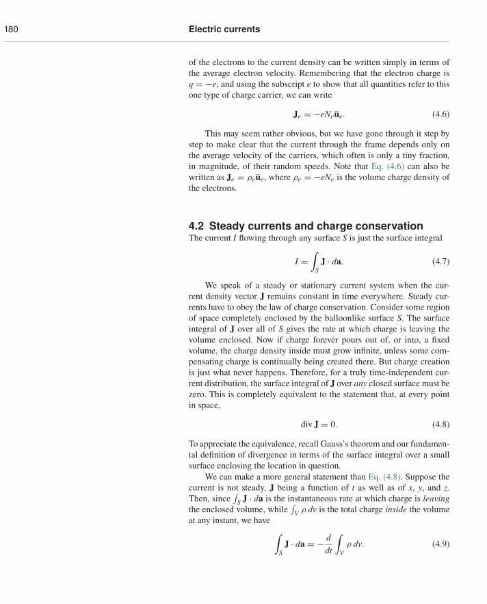
Example (Vacuum diode) An instructive example of a stationary currentdistribution occurs in the plane diode, a two-electrode vacuum tube; see Fig. 4.2.One electrode, the cathode, is coated with a material that emits electrons copi-
Cathode
Heater
Anode
v
x
y
E
Figure 4.2.A vacuum diode with plane-parallel cathode andanode.ously when heated. The other electrode, the anode, is simply a metal plate. By
means of a battery the anode is maintained at a positive potential with respectto the cathode. Electrons emerge from this hot cathode with very low velocitiesand then, being negatively charged, are accelerated toward the positive anode bythe electric field between cathode and anode. In the space between the cathodeand anode the electric current consists of these moving electrons. The circuit iscompleted by the flow of electrons in external wires, possibly by the movementof ions in a battery, and so on, with which we are not here concerned.
In this diode the local density of charge in any region, ρ, is simply −ne,where n is the local density of electrons, in electrons per cubic meter. The localcurrent density J is ρv, where v is the velocity of electrons in that region. In theplane-parallel diode we may assume J has no y or z components. If conditionsare steady, it follows then that Jx must be independent of x, for if div J = 0as Eq. (4.8) says, ∂Jx/∂x must be zero if Jy = Jz = 0. This is belaboringthe obvious; if we have a steady stream of electrons moving in the x direc-tion only, the same number per second have to cross any intermediate planebetween cathode and anode. We conclude that ρv is constant. But observe thatv is not constant; it varies with x because the electrons are accelerated by thefield. Hence ρ is not constant either. Instead, the negative charge density ishigh near the cathode and low near the anode, just as the density of cars onan expressway is high near a traffic slowdown and low where traffic is moving athigh speed.
4.3 Electrical conductivity and Ohm’s lawThere are many ways of causing charge to move, including what wemight call “bodily transport” of the charge carriers. In the Van de Graaff
2 If the step between Eqs. (4.9) and (4.10) is not obvious, look back at our fundamentaldefinition of divergence in Chapter 2. As the volume shrinks, we can eventually take ρ
outside the volume integral on the right. The volume integral is to be carried out at oneinstant of time. The time derivative thus depends on the difference between ρ
∫dv at t
and at t + dt. The only difference is due to the change of ρ there, since the boundary ofthe volume remains in the same place.
182 Electric currents
electrostatic generator (see Problem 4.1) an insulating belt is given a sur-face charge, which it conveys to another electrode for removal, much asan escalator conveys people. That constitutes a perfectly good current.In the atmosphere, charged water droplets falling because of their weightform a component of the electric current system of the earth. In this sec-tion we shall be interested in a more common agent of charge transport,the force exerted on a charge carrier by an electric field. An electric fieldE pushes positive charge carriers in one direction, negative charge car-riers in the opposite direction. If either or both can move, the result isan electric current in the direction of E. In most substances, and over awide range of electric field strengths, we find that the current density isproportional to the strength of the electric field that causes it. The linearrelation between current density and field is expressed by
J = σE (4.11)
The factor σ is called the conductivity of the material. Its value dependson the material in question; it is very large for metallic conductors,extremely small for good insulators. It may depend too on the physi-cal state of the material – on its temperature, for instance. But with suchconditions given, it does not depend on the magnitude of E. If you dou-ble the field strength, holding everything else constant, you get twice thecurrent density.
After everything we said in Chapter 3 about the electric field beingzero inside a conductor, you might be wondering why we are now talkingabout a nonzero internal field. The reason is that in Chapter 3 we weredealing with static situations, that is, ones in which all the charges havesettled down after some initial motion. In such a setup, the charges pileup at certain locations and create a field that internally cancels an appliedfield. But when dealing with currents in conductors, we are not letting thecharges pile up, which means that things can’t settle down. For example,a battery feeds in electrons at one end of a wire and takes them out at theother end. If the electrons were not taken out at the other end, then theywould pile up there, and the electric field would eventually (actually veryquickly) become zero inside.
The units of σ are the units of J (namely C s−1m−2) divided by theunits of E (namely V/m or N/C). You can quickly show that this yieldsC2 s kg−1m−3. However, it is customary to write the units of σ as thereciprocal of ohm-meter, (ohm-m)−1, where the ohm, which is the unitof resistance, is defined below.
In Eq. (4.11), σ may be considered a scalar quantity, implying thatthe direction of J is always the same as the direction of E. That is surelywhat we would expect within a material whose structure has no “built-in” preferred direction. Materials do exist in which the electrical con-ductivity itself depends on the angle the applied field E makes with
4.3 Electrical conductivity and Ohm’s law 183
some intrinsic axis in the material. One example is a single crystal ofgraphite, which has a layered structure on an atomic scale. For anotherexample, see Problem 4.5. In such cases J may not have the directionof E. But there still are linear relations between the components of J andthe components of E, relations expressed by Eq. (4.11) with σ a tensorquantity instead of a scalar.3 From now on we’ll consider only isotropicmaterials, those within which the electrical conductivity is the same inall directions.
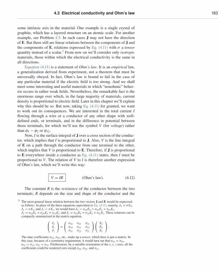
Equation (4.11) is a statement of Ohm’s law. It is an empirical law,a generalization derived from experiment, not a theorem that must beuniversally obeyed. In fact, Ohm’s law is bound to fail in the case ofany particular material if the electric field is too strong. And we shallmeet some interesting and useful materials in which “nonohmic” behav-ior occurs in rather weak fields. Nevertheless, the remarkable fact is theenormous range over which, in the large majority of materials, currentdensity is proportional to electric field. Later in this chapter we’ll explainwhy this should be so. But now, taking Eq. (4.11) for granted, we wantto work out its consequences. We are interested in the total current Iflowing through a wire or a conductor of any other shape with well-defined ends, or terminals, and in the difference in potential betweenthose terminals, for which we’ll use the symbol V (for voltage) ratherthan φ1 − φ2 or φ12.
Now, I is the surface integral of J over a cross section of the conduc-tor, which implies that I is proportional to J. Also, V is the line integralof E on a path through the conductor from one terminal to the other,which implies that V is proportional to E. Therefore, if J is proportionalto E everywhere inside a conductor as Eq. (4.11) states, then I must beproportional to V . The relation of V to I is therefore another expressionof Ohm’s law, which we’ll write this way:
V = IR (Ohm’s law). (4.12)
The constant R is the resistance of the conductor between the twoterminals; R depends on the size and shape of the conductor and the
3 The most general linear relation between the two vectors J and E would be expressedas follows. In place of the three equations equivalent to Eq. (4.11), namely, Jx = σEx,Jy = σEy, and Jz = σEz, we would have Jx = σxxEx + σxyEy + σxzEz,Jy = σyxEx + σyyEy + σyzEz, and Jz = σzxEx + σzyEy + σzzEz. These relations can becompactly summarized in the matrix equation,⎛
⎝ JxJyJz
⎞⎠ =
⎛⎝ σxx σxy σxz
σyx σyy σyzσzx σzy σzz
⎞⎠
⎛⎝ Ex
EyEz
⎞⎠ .
The nine coefficients σxx, σxy, etc., make up a tensor, which here is just a matrix. Inthis case, because of a symmetry requirement, it would turn out that σxy = σyx,σyz = σzy, σxz = σzx. Furthermore, by a suitable orientation of the x, y, z axes, all thecoefficients could be rendered zero except σxx, σyy, and σzz.
184 Electric currents
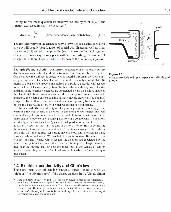
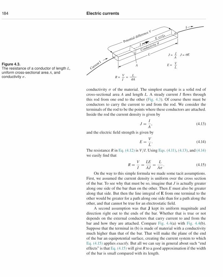
Figure 4.3.The resistance of a conductor of length L,uniform cross-sectional area A, andconductivity σ . L
sAVI
AI
R =
J =
E =
J =L
A
Potential difference V
Conductivity s
Current I
J
E
sE
=
VL
I
conductivity σ of the material. The simplest example is a solid rod ofcross-sectional area A and length L. A steady current I flows throughthis rod from one end to the other (Fig. 4.3). Of course there must beconductors to carry the current to and from the rod. We consider theterminals of the rod to be the points where these conductors are attached.Inside the rod the current density is given by
J = IA
, (4.13)
and the electric field strength is given by
E = VL
. (4.14)
The resistance R in Eq. (4.12) is V/I. Using Eqs. (4.11), (4.13), and (4.14)we easily find that
R = VI= LE
AJ= L
Aσ. (4.15)
On the way to this simple formula we made some tacit assumptions.First, we assumed the current density is uniform over the cross sectionof the bar. To see why that must be so, imagine that J is actually greateralong one side of the bar than on the other. Then E must also be greateralong that side. But then the line integral of E from one terminal to theother would be greater for a path along one side than for a path along theother, and that cannot be true for an electrostatic field.
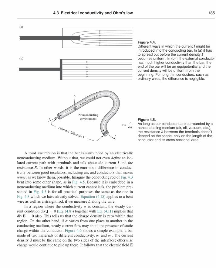
A second assumption was that J kept its uniform magnitude anddirection right out to the ends of the bar. Whether that is true or notdepends on the external conductors that carry current to and from thebar and how they are attached. Compare Fig. 4.4(a) with Fig. 4.4(b).Suppose that the terminal in (b) is made of material with a conductivitymuch higher than that of the bar. That will make the plane of the endof the bar an equipotential surface, creating the current system to whichEq. (4.15) applies exactly. But all we can say in general about such “endeffects” is that Eq. (4.15) will give R to a good approximation if the widthof the bar is small compared with its length.
4.3 Electrical conductivity and Ohm’s law 185
(a)
(b)
Figure 4.4.Different ways in which the current I might beintroduced into the conducting bar. In (a) it hasto spread out before the current density Jbecomes uniform. In (b) if the external conductorhas much higher conductivity than the bar, theend of the bar will be an equipotential and thecurrent density will be uniform from thebeginning. For long thin conductors, such asordinary wires, the difference is negligible.
Nonconductingenvironment
Potential difference V
Conductivity s
LsA
R =
A
I
I
L
Figure 4.5.As long as our conductors are surrounded by anonconducting medium (air, oil, vacuum, etc.),the resistance R between the terminals doesn’tdepend on the shape, only on the length of theconductor and its cross-sectional area.
A third assumption is that the bar is surrounded by an electricallynonconducting medium. Without that, we could not even define an iso-lated current path with terminals and talk about the current I and theresistance R. In other words, it is the enormous difference in conduc-tivity between good insulators, including air, and conductors that makeswires, as we know them, possible. Imagine the conducting rod of Fig. 4.3bent into some other shape, as in Fig. 4.5. Because it is embedded in anonconducting medium into which current cannot leak, the problem pre-sented in Fig. 4.5 is for all practical purposes the same as the one inFig. 4.3 which we have already solved. Equation (4.15) applies to a bentwire as well as a straight rod, if we measure L along the wire.
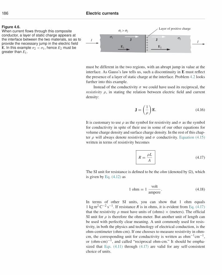
In a region where the conductivity σ is constant, the steady cur-rent condition div J = 0 (Eq. (4.8)) together with Eq. (4.11) implies thatdiv E = 0 also. This tells us that the charge density is zero within thatregion. On the other hand, if σ varies from one place to another in theconducting medium, steady current flow may entail the presence of staticcharge within the conductor. Figure 4.6 shows a simple example, a barmade of two materials of different conductivity, σ1 and σ2. The currentdensity J must be the same on the two sides of the interface; otherwisecharge would continue to pile up there. It follows that the electric field E
186 Electric currents
Figure 4.6.When current flows through this compositeconductor, a layer of static charge appears atthe interface between the two materials, so as toprovide the necessary jump in the electric fieldE. In this example σ2 < σ1, hence E2 must begreater than E1.
s1 > s2
s1 s2
E1 E2
I IJ
Layer of positive charge
J ++++++
must be different in the two regions, with an abrupt jump in value at theinterface. As Gauss’s law tells us, such a discontinuity in E must reflectthe presence of a layer of static charge at the interface. Problem 4.2 looksfurther into this example.
Instead of the conductivity σ we could have used its reciprocal, theresistivity ρ, in stating the relation between electric field and currentdensity:
J =(
1ρ
)E. (4.16)
It is customary to use ρ as the symbol for resistivity and σ as the symbolfor conductivity in spite of their use in some of our other equations forvolume charge density and surface charge density. In the rest of this chap-ter ρ will always denote resistivity and σ conductivity. Equation (4.15)written in terms of resistivity becomes
R = ρLA
(4.17)
The SI unit for resistance is defined to be the ohm (denoted by �), whichis given by Eq. (4.12) as
1 ohm = 1volt
ampere. (4.18)
In terms of other SI units, you can show that 1 ohm equals1 kg m2 C−2 s−1. If resistance R is in ohms, it is evident from Eq. (4.17)that the resistivity ρ must have units of (ohms) × (meters). The officialSI unit for ρ is therefore the ohm-meter. But another unit of length canbe used with perfectly clear meaning. A unit commonly used for resis-tivity, in both the physics and technology of electrical conduction, is theohm-centimeter (ohm-cm). If one chooses to measure resistivity in ohm-cm, the corresponding unit for conductivity is written as ohm−1cm−1,or (ohm-cm)−1, and called “reciprocal ohm-cm.” It should be empha-sized that Eqs. (4.11) through (4.17) are valid for any self-consistentchoice of units.
4.3 Electrical conductivity and Ohm’s law 187
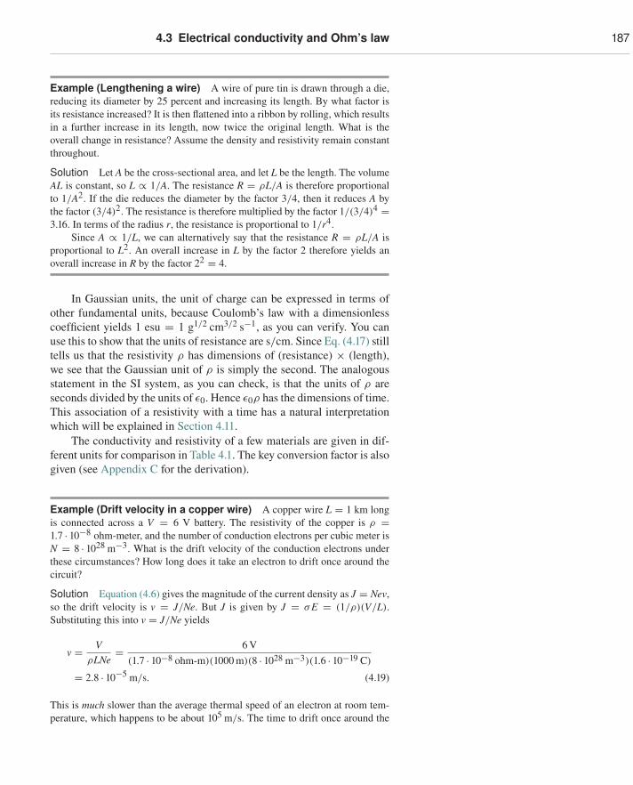
Example (Lengthening a wire) A wire of pure tin is drawn through a die,reducing its diameter by 25 percent and increasing its length. By what factor isits resistance increased? It is then flattened into a ribbon by rolling, which resultsin a further increase in its length, now twice the original length. What is theoverall change in resistance? Assume the density and resistivity remain constantthroughout.
Solution Let A be the cross-sectional area, and let L be the length. The volumeAL is constant, so L ∝ 1/A. The resistance R = ρL/A is therefore proportionalto 1/A2. If the die reduces the diameter by the factor 3/4, then it reduces A bythe factor (3/4)2. The resistance is therefore multiplied by the factor 1/(3/4)4 =3.16. In terms of the radius r, the resistance is proportional to 1/r4.
Since A ∝ 1/L, we can alternatively say that the resistance R = ρL/A isproportional to L2. An overall increase in L by the factor 2 therefore yields anoverall increase in R by the factor 22 = 4.
In Gaussian units, the unit of charge can be expressed in terms ofother fundamental units, because Coulomb’s law with a dimensionlesscoefficient yields 1 esu = 1 g1/2 cm3/2 s−1, as you can verify. You canuse this to show that the units of resistance are s/cm. Since Eq. (4.17) stilltells us that the resistivity ρ has dimensions of (resistance) × (length),we see that the Gaussian unit of ρ is simply the second. The analogousstatement in the SI system, as you can check, is that the units of ρ areseconds divided by the units of ε0. Hence ε0ρ has the dimensions of time.This association of a resistivity with a time has a natural interpretationwhich will be explained in Section 4.11.
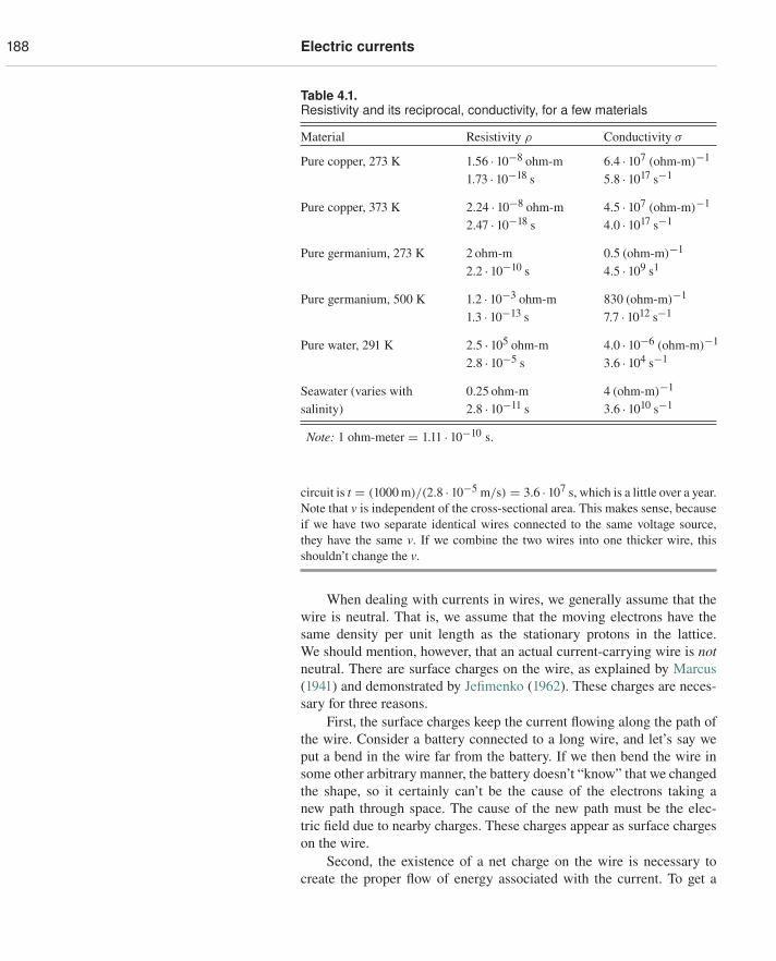
The conductivity and resistivity of a few materials are given in dif-ferent units for comparison in Table 4.1. The key conversion factor is alsogiven (see Appendix C for the derivation).
Example (Drift velocity in a copper wire) A copper wire L = 1 km longis connected across a V = 6 V battery. The resistivity of the copper is ρ =1.7 · 10−8 ohm-meter, and the number of conduction electrons per cubic meter isN = 8 · 1028 m−3. What is the drift velocity of the conduction electrons underthese circumstances? How long does it take an electron to drift once around thecircuit?
Solution Equation (4.6) gives the magnitude of the current density as J = Nev,so the drift velocity is v = J/Ne. But J is given by J = σE = (1/ρ)(V/L).Substituting this into v = J/Ne yields
v = VρLNe
= 6 V(1.7 · 10−8 ohm-m)(1000 m)(8 · 1028 m−3)(1.6 · 10−19 C)
= 2.8 · 10−5 m/s. (4.19)
This is much slower than the average thermal speed of an electron at room tem-perature, which happens to be about 105 m/s. The time to drift once around the
188 Electric currents
Table 4.1.Resistivity and its reciprocal, conductivity, for a few materials
Material Resistivity ρ Conductivity σ
Pure copper, 273 K 1.56 · 10−8 ohm-m 6.4 · 107 (ohm-m)−1
1.73 · 10−18 s 5.8 · 1017 s−1
Pure copper, 373 K 2.24 · 10−8 ohm-m 4.5 · 107 (ohm-m)−1
2.47 · 10−18 s 4.0 · 1017 s−1
Pure germanium, 273 K 2 ohm-m 0.5 (ohm-m)−1
2.2 · 10−10 s 4.5 · 109 s1
Pure germanium, 500 K 1.2 · 10−3 ohm-m 830 (ohm-m)−1
1.3 · 10−13 s 7.7 · 1012 s−1
Pure water, 291 K 2.5 · 105 ohm-m 4.0 · 10−6 (ohm-m)−1
2.8 · 10−5 s 3.6 · 104 s−1
Seawater (varies with 0.25 ohm-m 4 (ohm-m)−1
salinity) 2.8 · 10−11 s 3.6 · 1010 s−1
Note: 1 ohm-meter = 1.11 · 10−10 s.
circuit is t = (1000 m)/(2.8 · 10−5 m/s) = 3.6 · 107 s, which is a little over a year.Note that v is independent of the cross-sectional area. This makes sense, becauseif we have two separate identical wires connected to the same voltage source,they have the same v. If we combine the two wires into one thicker wire, thisshouldn’t change the v.
When dealing with currents in wires, we generally assume that thewire is neutral. That is, we assume that the moving electrons have thesame density per unit length as the stationary protons in the lattice.We should mention, however, that an actual current-carrying wire is notneutral. There are surface charges on the wire, as explained by Marcus(1941) and demonstrated by Jefimenko (1962). These charges are neces-sary for three reasons.
First, the surface charges keep the current flowing along the path ofthe wire. Consider a battery connected to a long wire, and let’s say weput a bend in the wire far from the battery. If we then bend the wire insome other arbitrary manner, the battery doesn’t “know” that we changedthe shape, so it certainly can’t be the cause of the electrons taking anew path through space. The cause of the new path must be the elec-tric field due to nearby charges. These charges appear as surface chargeson the wire.
Second, the existence of a net charge on the wire is necessary tocreate the proper flow of energy associated with the current. To get a
4.4 The physics of electrical conduction 189
handle on this energy flow, we will have to wait until we learn aboutmagnetic fields in Chapter 6 and the Poynting vector in Chapter 9. Butfor now we’ll just say that to have the proper energy flow, there must bea component of the electric field pointing radially away from the wire.This component wouldn’t exist if the net charge on the wire were zero.
Third, the surface charge causes the potential to change along thewire in a manner consistent with Ohm’s law. See Jackson (1996) for morediscussion on these three roles that the surface charges play.
However, having said all this, it turns out that in most of our discus-sions of circuits and currents in this book, we won’t be interested in theelectric field external to the wires. So we can generally ignore the surfacecharges, with no ill effects.
4.4 The physics of electrical conduction4.4.1 Currents and ionsTo explain electrical conduction we have to talk first about atoms andmolecules. Remember that a neutral atom, one that contains as manyelectrons as there are protons in its nucleus, is precisely neutral (seeSection 1.3). On such an object the net force exerted by an electric fieldis exactly zero. And even if the neutral atom were moved along by someother means, that would not be an electric current. The same holds forneutral molecules. Matter that consists only of neutral molecules oughtto have zero electrical conductivity. Here one qualification is in order:we are concerned now with steady electric currents, that is, direct cur-rents, not alternating currents. An alternating electric field could causeperiodic deformation of a molecule, and that displacement of electriccharge would be a true alternating electric current. We shall return tothat subject in Chapter 10. For a steady current we need mobile chargecarriers, or ions. These must be present in the material before the elec-tric field is applied, for the electric fields we shall consider are not nearlystrong enough to create ions by tearing electrons off molecules. Thus thephysics of electrical conduction centers on two questions: how many ionsare there in a unit volume of material, and how do these ions move in thepresence of an electric field?
In pure water at room temperature approximately two H2O moleculesin a billion are, at any given moment, dissociated into negative ions,OH−, and positive ions, H+. (Actually the positive ion is better describedas OH+
3 , that is, a proton attached to a water molecule.) This providesapproximately 6 · 1013 negative ions and an equal number of positiveions in a cubic centimeter of water.4 The motion of these ions in the
4 Students of chemistry may recall that the concentration of hydrogen ions in pure watercorresponds to a pH value of 7.0, which means the concentration is 10−7.0 mole/liter.That is equivalent to 10−10.0 mole/cm3. A mole of anything is 6.02 · 1023 things –hence the number 6 · 1013 given above.
190 Electric currents
applied electric field accounts for the conductivity of pure water givenin Table 4.1. Adding a substance like sodium chloride, whose moleculeseasily dissociate in water, can increase enormously the number of ions.That is why seawater has electrical conductivity nearly a million timesgreater than that of pure water. It contains something like 1020 ions percubic centimeter, mostly Na+ and Cl−.
In a gas like nitrogen or oxygen at ordinary temperatures there wouldbe no ions at all except for the action of some ionizing radiation suchas ultraviolet light, x-rays, or nuclear radiation. For instance, ultravioletlight might eject an electron from a nitrogen molecule, leaving N+
2 , amolecular ion with a positive charge e. The electron thus freed is a neg-ative ion. It may remain free or it may eventually stick to some moleculeas an “extra” electron, thus forming a negative molecular ion. The oxy-gen molecule happens to have an especially high affinity for an extraelectron; when air is ionized, N+
2 and O−2 are common ion types. In any
case, the resulting conductivity of the gas depends on the number ofions present at any moment, which depends in turn on the intensity ofthe ionizing radiation and perhaps other circumstances as well. So wecannot find in a table the conductivity of a gas. Strictly speaking, theconductivity of pure nitrogen shielded from all ionizing radiation wouldbe zero.5
Given a certain concentration of positive and negative ions in amaterial, how is the resulting conductivity, σ in Eq. (4.11), determined?Let’s consider first a slightly ionized gas. To be specific, suppose its den-sity is like that of air in a room – about 1025 molecules per cubic meter.Here and there among these neutral molecules are positive and negativeions. Suppose there are N positive ions in unit volume, each of mass M+and carrying charge e, and an equal number of negative ions, each withmass M− and charge −e. The number of ions in unit volume, 2N, is verymuch smaller than the number of neutral molecules. When an ion col-lides with anything, it is almost always a neutral molecule rather thananother ion. Occasionally a positive ion does encounter a negative ionand combine with it to form a neutral molecule. Such recombination6
would steadily deplete the supply of ions if ions were not being continu-ally created by some other process. But in any case the rate of change ofN will be so slow that we can neglect it here.
5 But what about thermal energy? Won’t that occasionally lead to the ionization of amolecule? In fact, the energy required to ionize, that is, to extract an electron from, anitrogen molecule is several hundred times the mean thermal energy of a molecule at300 K. You would not expect to find even one ion so produced in the entire earth’satmosphere!
6 In calling the process recombination we of course do not wish to imply that the two“recombining” ions were partners originally. Close encounters of a positive ion with anegative ion are made somewhat more likely by their electrostatic attraction. However,that effect is generally not important when the number of ions per unit volume is verymuch smaller than the number of neutral molecules.
4.4 The physics of electrical conduction 191
4.4.2 Motion in zero electric fieldImagine now the scene, on a molecular scale, before an electric field isapplied. The molecules, and the ions too, are flying about with randomvelocities appropriate to the temperature. The gas is mostly empty space,the mean distance between a molecule and its nearest neighbor beingabout ten molecular diameters. The mean free path of a molecule, whichis the average distance it travels before bumping into another molecule,is much larger, perhaps 10−7 m, or several hundred molecular diam-eters. A molecule or an ion in this gas spends 99.9 percent of its timeas a free particle. If we could look at a particular ion at a particularinstant, say t = 0, we would find it moving through space with somevelocity u.
What will happen next? The ion will move in a straight line at con-stant speed until, sooner or later, it chances to come close to a molecule,close enough for strong short-range forces to come into play. In this col-lision the total kinetic energy and the total momentum of the two bod-ies, molecule and ion, will be conserved, but the ion’s velocity will berather suddenly changed in both magnitude and direction to some newvelocity u′. It will then coast along freely with this new velocity untilanother collision changes its velocity to u′′, and so on. After at most afew such collisions the ion is as likely to be moving in any direction asin any other direction. The ion will have “forgotten” the direction it wasmoving at t = 0.
To put it another way, if we picked 10,000 cases of ions moving hor-izontally south, and followed each of them for a sufficient time of τ sec-onds, their final velocity directions would be distributed impartially overa sphere. It may take several collisions to wipe out most of the directionmemory or only a few, depending on whether collisions involving smallmomentum changes or large momentum changes are the more common,and this depends on the nature of the interaction. An extreme case isthe collision of hard elastic spheres, which turns out to produce a com-pletely random new direction in just one collision. We need not worryabout these differences. The point is that, whatever the nature of the colli-sions, there will be some time interval τ , characteristic of a given system,such that the lapse of τ seconds leads to substantial loss of correlationbetween the initial velocity direction and the final velocity direction ofan ion in that system.7 This characteristic time τ will depend on the ionand on the nature of its average environment; it will certainly be shorterthe more frequent the collisions, since in our gas nothing happens to anion between collisions.
7 It would be possible to define τ precisely for a general system by giving a quantitativemeasure of the correlation between initial and final directions. It is a statisticalproblem, like devising a measure of the correlation between the birth weights of ratsand their weights at maturity. However, we shall not need a general quantitativedefinition to complete our analysis.
192 Electric currents
4.4.3 Motion in nonzero electric fieldNow we are ready to apply a uniform electric field E to the system.It will make the description easier if we imagine the loss of directionmemory to occur completely at a single collision, as we have said itdoes in the case of hard spheres. Our main conclusion will actuallybe independent of this assumption. Immediately after a collision an ionstarts off in some random direction. We will denote by uc the velocityimmediately after a collision. The electric force Ee on the ion impartsmomentum to the ion continuously. After time t it will have acquiredfrom the field a momentum increment Eet, which simply adds vectori-ally to its original momentum Muc. Its momentum is now Muc + Eet.If the momentum increment is small relative to Muc, that implies thatthe velocity has not been affected much, so we can expect the next col-lision to occur about as soon as it would have in the absence of theelectric field. In other words, the average time between collisions, whichwe shall denote by t, is independent of the field E if the field is nottoo strong.
The momentum acquired from the field is always a vector in thesame direction. But it is lost, in effect, at every collision, since the direc-tion of motion after a collision is random, regardless of the directionbefore.
What is the average momentum of all the positive ions at a giveninstant of time? This question is surprisingly easy to answer if we look atit this way. At the instant in question, suppose we stop the clock and askeach ion how long it has been since its last collision. Suppose we get theparticular answer t1 from positive ion 1. Then that ion must have momen-tum eEt1 in addition to the momentum Muc
1 with which it emergedfrom its last collision. The average momentum of all N positive ions istherefore
Mu+ = 1N
∑j
(Muc
j + eEtj). (4.20)
Here ucj is the velocity the jth ion had just after its last collision. These
velocities ucj are quite random in direction and therefore contribute zero
to the average. The second part is simply Ee times the average of the tj,that is, times the average of the time since the last collision. That mustbe the same as the average of the time until the next collision, and bothare the same8 as the average time between collisions, t. We conclude
8 You may think the average time between collisions would have to be equal to the sumof the average time since the last collision and the average time to the next. That wouldbe true if collisions occurred at absolutely regular intervals, but they don’t. They areindependent random events, and for such the above statement, paradoxical as it mayseem at first, is true. Think about it. The question does not affect our main conclusion,but if you unravel it you will have grown in statistical wisdom; see Exercise 4.23.(Hint: If one collision doesn’t affect the probability of having another – that’s whatindependent means – it can’t matter whether you start the clock at some arbitrary time,or at the time of a collision.)
4.4 The physics of electrical conduction 193
that the average velocity of a positive ion, in the presence of the steadyfield E, is
u+ = Eet+M+
. (4.21)
This shows that the average velocity of a charge carrier is proportionalto the electric force applied to it. If we observe only the average velocity,it looks as if the medium were resisting the motion with a force pro-portional to the velocity. This is true because if we write Eq. (4.21) asEe − (M+/t+)u+ = 0, we can interpret it as the terminal-velocity state-ment that the Ee electric force is balanced by a −bu+ drag force, whereb ≡ M+/t+. This −bu force is the kind of frictional drag you feel if youtry to stir thick syrup with a spoon, a “viscous” drag. Whenever chargecarriers behave like this, we can expect something like Ohm’s law, forthe following reason.
In Eq. (4.21) we have written t+ because the mean time betweencollisions may well be different for positive and negative ions. The neg-ative ions acquire velocity in the opposite direction, but since they carrynegative charge their contribution to the current density J adds to thatof the positives. The equivalent of Eq. (4.6), with the two sorts of ionsincluded, is now
J = Ne(
eEt+M+
)− Ne
(−eEt−M−
)= Ne2
(t+
M++ t−
M−
)E. (4.22)
Our theory therefore predicts that the system will obey Ohm’s law, forEq. (4.22) expresses a linear relation between J and E, the other quan-tities being constants characteristic of the medium. Compare Eq. (4.22)with Eq. (4.11). The constant Ne2(t+/M+ + t−/M−) appears in the roleof σ , the conductivity.
We made a number of rather special assumptions about this sys-tem, but looking back, we can see that they were not essential so far asthe linear relation between E and J is concerned. Any system contain-ing a constant density of free charge carriers, in which the motion ofthe carriers is frequently “re-randomized” by collisions or other interac-tions within the system, ought to obey Ohm’s law if the field E is not toostrong. The ratio of J to E, which is the conductivity σ of the medium,will be proportional to the number of charge carriers and to the char-acteristic time τ , the time for loss of directional correlation. It is onlythrough this last quantity that all the complicated details of the collisionsenter the problem. The making of a detailed theory of the conductivityof any given system, assuming the number of charge carriers is known,amounts to making a theory for τ . In our particular example this quan-tity was replaced by t, and a perfectly definite result was predicted forthe conductivity σ . Introducing the more general quantity τ , and also
194 Electric currents
allowing for the possibility of different numbers of positive and negativecarriers, we can summarize our theory as follows:
σ ≈ e2(
N+τ+M+
+ N−τ−M−
)(4.23)
We use the ≈ sign to acknowledge that we did not give τ a precise defi-nition. That could be done, however.
Example (Atmospheric conductivity) Normally in the earth’s atmospherethe greatest density of free electrons (liberated by ultraviolet sunlight) amountsto 1012 per cubic meter and is found at an altitude of about 100 km where thedensity of air is so low that the mean free path of an electron is about 0.1 m. Atthe temperature that prevails there, an electron’s mean speed is 105 m/s. What isthe conductivity in (ohm-m)−1?
Solution We have only one type of charge carrier, so Eq. (4.23) gives the con-ductivity as σ = Ne2τ/m. The mean free time is τ = (0.1 m)/(105 m/s) =10−6 s. Therefore,
σ = Ne2τ
m= (1012 m−3)(1.6 · 10−19 C)2(10−6 s)
9.1 · 10−31 kg= 0.028 (ohm-m)−1.
(4.24)
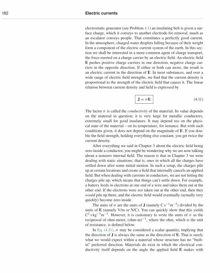
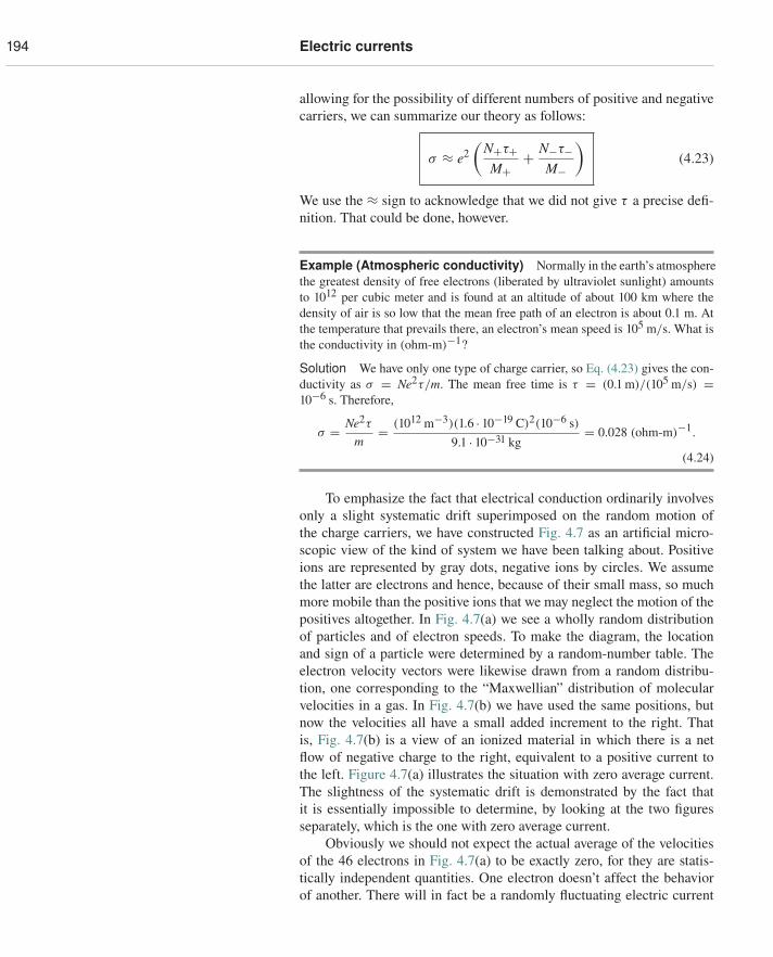
To emphasize the fact that electrical conduction ordinarily involvesonly a slight systematic drift superimposed on the random motion ofthe charge carriers, we have constructed Fig. 4.7 as an artificial micro-scopic view of the kind of system we have been talking about. Positiveions are represented by gray dots, negative ions by circles. We assumethe latter are electrons and hence, because of their small mass, so muchmore mobile than the positive ions that we may neglect the motion of thepositives altogether. In Fig. 4.7(a) we see a wholly random distributionof particles and of electron speeds. To make the diagram, the locationand sign of a particle were determined by a random-number table. Theelectron velocity vectors were likewise drawn from a random distribu-tion, one corresponding to the “Maxwellian” distribution of molecularvelocities in a gas. In Fig. 4.7(b) we have used the same positions, butnow the velocities all have a small added increment to the right. Thatis, Fig. 4.7(b) is a view of an ionized material in which there is a netflow of negative charge to the right, equivalent to a positive current tothe left. Figure 4.7(a) illustrates the situation with zero average current.The slightness of the systematic drift is demonstrated by the fact thatit is essentially impossible to determine, by looking at the two figuresseparately, which is the one with zero average current.
Obviously we should not expect the actual average of the velocitiesof the 46 electrons in Fig. 4.7(a) to be exactly zero, for they are statis-tically independent quantities. One electron doesn’t affect the behaviorof another. There will in fact be a randomly fluctuating electric current
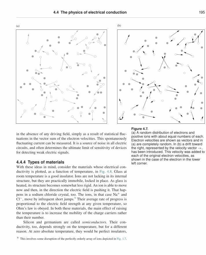
4.4 The physics of electrical conduction 195
(b)(a)
Figure 4.7.(a) A random distribution of electrons andpositive ions with about equal numbers of each.Electron velocities are shown as vectors and in(a) are completely random. In (b) a drift towardthe right, represented by the velocity vector →,has been introduced. This velocity was added toeach of the original electron velocities, asshown in the case of the electron in the lowerleft corner.
in the absence of any driving field, simply as a result of statistical fluc-tuations in the vector sum of the electron velocities. This spontaneouslyfluctuating current can be measured. It is a source of noise in all electriccircuits, and often determines the ultimate limit of sensitivity of devicesfor detecting weak electric signals.
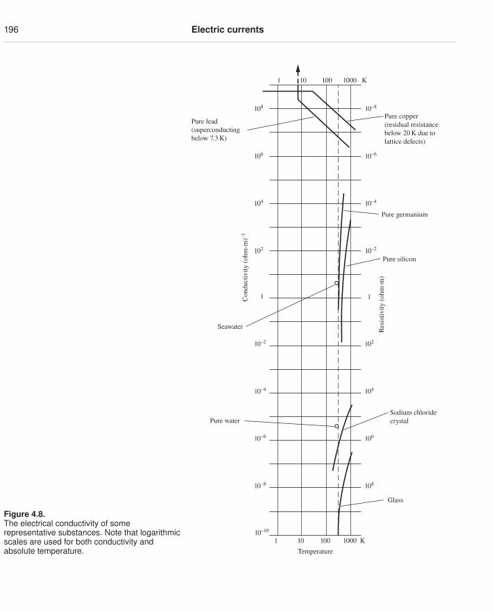
4.4.4 Types of materialsWith these ideas in mind, consider the materials whose electrical con-ductivity is plotted, as a function of temperature, in Fig. 4.8. Glass atroom temperature is a good insulator. Ions are not lacking in its internalstructure, but they are practically immobile, locked in place. As glass isheated, its structure becomes somewhat less rigid. An ion is able to movenow and then, in the direction the electric field is pushing it. That hap-pens in a sodium chloride crystal, too. The ions, in that case Na+ andCl−, move by infrequent short jumps.9 Their average rate of progress isproportional to the electric field strength at any given temperature, soOhm’s law is obeyed. In both these materials, the main effect of raisingthe temperature is to increase the mobility of the charge carriers ratherthan their number.
Silicon and germanium are called semiconductors. Their con-ductivity, too, depends strongly on the temperature, but for a differentreason. At zero absolute temperature, they would be perfect insulators,
9 This involves some disruption of the perfectly orderly array of ions depicted in Fig. 1.7.
196 Electric currents
Figure 4.8.The electrical conductivity of somerepresentative substances. Note that logarithmicscales are used for both conductivity andabsolute temperature.
1 10 100 1000 K
Temperature
Glass
10–10
10–8
10–6
10–4
10–2
Seawater
Pure water
1
108
106
104
102
10–4104
10–2102C
ondu
ctiv
ity (o
hm-m
)–1
106
108
1 10 100 1000 K
10–6
10–8
Pure copper(residual resistancebelow 20 K due tolattice defects)
Pure lead(superconductingbelow 7.3 K)
Pure germanium
Pure silicon
Sodium chloridecrystal
Res
istiv
ity (o
hm-m
)
1
4.4 The physics of electrical conduction 197
containing no ions at all, only neutral atoms. The effect of thermal energyis to create charge carriers by liberating electrons from some of theatoms. The steep rise in conductivity around room temperature and abovereflects a great increase in the number of mobile electrons, not an increasein the mobility of an individual electron. We shall look more closely atsemiconductors in Section 4.6.
The metals, exemplified by copper and lead in Fig. 4.8, are even bet-ter conductors. Their conductivity generally decreases with increasingtemperature, due to an effect we will discuss in Section 4.5. In fact, overmost of the range plotted, the conductivity of a pure metal like copperor lead is inversely proportional to the absolute temperature, as can beseen from the 45◦ slope of our logarithmic graph. Were that behaviorto continue as copper and lead are cooled down toward absolute zero,we could expect an enormous increase in conductivity. At 0.001 K, atemperature readily attainable in the laboratory, we should expect theconductivity of each metal to rise to 300,000 times its room tempera-ture value. In the case of copper, we would be sadly disappointed. Aswe cool copper below about 20 K, its conductivity ceases to rise andremains constant from there on down. We will try to explain that inSection 4.5.
In the case of lead, normally a somewhat poorer conductor than cop-per, something far more surprising happens. As a lead wire is cooledbelow 7.2 K, its resistance abruptly and completely vanishes. The metalbecomes superconducting. This means, among other things, that an elec-tric current, once started flowing in a circuit of lead wire, will continueto flow indefinitely (for years, even!) without any electric field to driveit. The conductivity may be said to be infinite, though the concept reallyloses its meaning in the superconducting state. Warmed above 7.2 K, thelead wire recovers its normal resistance as abruptly as it lost it. Manymetals can become superconductors. The temperature at which the tran-sition from the normal to the superconducting state occurs depends onthe material. In high-temperature superconductors, transitions as high as130 K have been observed.
Our model of ions accelerated by the electric field, their progressbeing continually impeded by collisions, utterly fails us here. Somehow,in the superconducting state all impediment to the electrons’ motion hasvanished. Not only that, magnetic effects just as profound and mysteriousare manifest in the superconductor. At this stage of our study we cannotfully describe, let alone explain, the phenomenon of superconductivity.More will be said in Appendix I, which should be intelligible after ourstudy of magnetism.
Superconductivity aside, all these materials obey Ohm’s law. Dou-bling the electric field doubles the current if other conditions, includ-ing the temperature, are held constant. At least that is true if the fieldis not too strong. It is easy to see how Ohm’s law could fail in the caseof a partially ionized gas. Suppose the electric field is so strong that the
198 Electric currents
additional velocity an electron acquires between collisions is comparableto its thermal velocity. Then the time between collisions will be shorterthan it was before the field was applied, an effect not included in our the-ory and one that will cause the observed conductivity to depend on thefield strength.
A more spectacular breakdown of Ohm’s law occurs if the electricfield is further increased until an electron gains so much energy betweencollisions that in striking a neutral atom it can knock another electronloose. The two electrons can now release still more electrons in the sameway. Ionization increases explosively, quickly making a conducting pathbetween the electrodes. This is a spark. It’s what happens when a spark-plug fires, and when you touch a doorknob after walking over a rug ona dry day. There are always a few electrons in the air, liberated by cos-mic rays if in no other way. Since one electron is enough to trigger aspark, this sets a practical limit to field strength that can be maintainedin a gas. Air at atmospheric pressure will break down at roughly 3 mega-volts/meter. In a gas at low pressure, where an electron’s free path isquite long, as within the tube of an ordinary fluorescent lamp, a steadycurrent can be maintained with a modest field, with ionization by elec-tron impact occurring at a constant rate. The physics is fairly complex,and the behavior far from ohmic.
4.5 Conduction in metalsThe high conductivity of metals is due to electrons within the metal thatare not attached to atoms but are free to move through the whole solid.Proof of this is the fact that electric current in a copper wire – unlikecurrent in an ionic solution – transports no chemically identifiable sub-stance. A current can flow steadily for years without causing the slightestchange in the wire. It could only be electrons that are moving, enteringthe wire at one end and leaving it at the other.
We know from chemistry that atoms of the metallic elements rathereasily lose their outermost electrons.10 These would be bound to theatom if it were isolated, but become detached when many such atomsare packed close together in a solid. The atoms thus become positiveions, and these positive ions form the rigid lattice of the solid metal,usually in an orderly array. The detached electrons, which we shall callthe conduction electrons, move through this three-dimensional lattice ofpositive ions.
The number of conduction electrons is large. The metal sodium, forinstance, contains 2.5 · 1022 atoms in 1 cm3, and each atom provides oneconduction electron. No wonder sodium is a good conductor! But wait,there is a deep puzzle here. It is brought to light by applying our simple
10 This could even be taken as the property that defines a metallic element, makingsomewhat tautological the statement that metals are good conductors.
4.5 Conduction in metals 199
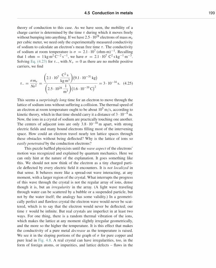
theory of conduction to this case. As we have seen, the mobility of acharge carrier is determined by the time τ during which it moves freelywithout bumping into anything. If we have 2.5 · 1028 electrons of mass meper cubic meter, we need only the experimentally measured conductivityof sodium to calculate an electron’s mean free time τ . The conductivityof sodium at room temperature is σ = 2.1 · 107 (ohm-m)−1. Recallingthat 1 ohm = 1 kg m2 C−2 s−1, we have σ = 2.1 · 107 C2 s kg−1 m−3.Solving Eq. (4.23) for τ−, with N+ = 0 as there are no mobile positivecarriers, we find
τ− = σme
Ne2 =
(2.1 · 107 C2 s
kg m3
)(9.1 · 10−31 kg
)(
2.5 · 1028 1m3
)(1.6 · 10−19 C
)2= 3 · 10−14 s. (4.25)
This seems a surprisingly long time for an electron to move through thelattice of sodium ions without suffering a collision. The thermal speed ofan electron at room temperature ought to be about 105 m/s, according tokinetic theory, which in that time should carry it a distance of 3 · 10−9 m.Now, the ions in a crystal of sodium are practically touching one another.The centers of adjacent ions are only 3.8 · 10−10 m apart, with strongelectric fields and many bound electrons filling most of the interveningspace. How could an electron travel nearly ten lattice spaces throughthese obstacles without being deflected? Why is the lattice of ions soeasily penetrated by the conduction electrons?
This puzzle baffled physicists until the wave aspect of the electrons’motion was recognized and explained by quantum mechanics. Here wecan only hint at the nature of the explanation. It goes something likethis. We should not now think of the electron as a tiny charged parti-cle deflected by every electric field it encounters. It is not localized inthat sense. It behaves more like a spread-out wave interacting, at anymoment, with a larger region of the crystal. What interrupts the progressof this wave through the crystal is not the regular array of ions, densethough it is, but an irregularity in the array. (A light wave travelingthrough water can be scattered by a bubble or a suspended particle, butnot by the water itself; the analogy has some validity.) In a geometri-cally perfect and flawless crystal the electron wave would never be scat-tered, which is to say that the electron would never be deflected; ourtime τ would be infinite. But real crystals are imperfect in at least twoways. For one thing, there is a random thermal vibration of the ions,which makes the lattice at any moment slightly irregular geometrically,and the more so the higher the temperature. It is this effect that makesthe conductivity of a pure metal decrease as the temperature is raised.We see it in the sloping portions of the graph of σ for pure copper andpure lead in Fig. 4.8. A real crystal can have irregularities, too, in theform of foreign atoms, or impurities, and lattice defects – flaws in the
200 Electric currents
stacking of the atomic array. Scattering by these irregularities limits thefree time τ whatever the temperature. Such defects are responsible for theresidual temperature-independent resistivity seen in the plot for copperin Fig. 4.8.
In metals Ohm’s law is obeyed exceedingly accurately up to cur-rent densities far higher than any that can be long maintained. No devi-ation has ever been clearly demonstrated experimentally. According toone theoretical prediction, departures on the order of 1 percent might beexpected at a current density of 1013 A/m2. That is more than a milliontimes the current density typical of wires in ordinary circuits.
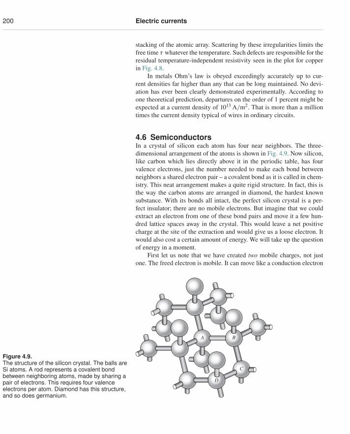
4.6 SemiconductorsIn a crystal of silicon each atom has four near neighbors. The three-dimensional arrangement of the atoms is shown in Fig. 4.9. Now silicon,like carbon which lies directly above it in the periodic table, has fourvalence electrons, just the number needed to make each bond betweenneighbors a shared electron pair – a covalent bond as it is called in chem-istry. This neat arrangement makes a quite rigid structure. In fact, this isthe way the carbon atoms are arranged in diamond, the hardest knownsubstance. With its bonds all intact, the perfect silicon crystal is a per-fect insulator; there are no mobile electrons. But imagine that we couldextract an electron from one of these bond pairs and move it a few hun-dred lattice spaces away in the crystal. This would leave a net positivecharge at the site of the extraction and would give us a loose electron. Itwould also cost a certain amount of energy. We will take up the questionof energy in a moment.
First let us note that we have created two mobile charges, not justone. The freed electron is mobile. It can move like a conduction electron
Figure 4.9.The structure of the silicon crystal. The balls areSi atoms. A rod represents a covalent bondbetween neighboring atoms, made by sharing apair of electrons. This requires four valenceelectrons per atom. Diamond has this structure,and so does germanium.
A B
C
D
4.6 Semiconductors 201
in a metal, like which it is spread out, not sharply localized. The quan-tum state it occupies we call a state in the conduction band. The positivecharge left behind is also mobile. If you think of it as an electron miss-ing in the bond between atoms A and B in Fig. 4.9, you can see that thisvacancy among the valence electrons could be transferred to the bondbetween B and C, thence to the bond between C and D, and so on, justby shifting electrons from one bond to another. Actually, the motion ofthe hole, as we shall call it henceforth, is even freer than this would sug-gest. It sails through the lattice like a conduction electron. The differenceis that it is a positive charge. An electric field E accelerates the hole inthe direction of E, not the reverse. The hole acts as if it had a mass com-parable with an electron’s mass. This is really rather mysterious, for thehole’s motion results from the collective motion of many valence elec-trons.11 Nevertheless, and fortunately, it acts so much like a real positiveparticle that we may picture it as such from now on.
The minimum energy required to extract an electron from a valencestate in silicon and leave it in the conduction band is 1.8 · 10−19 joule, or1.12 electron-volts (eV). One electron-volt is the work done in movingone electronic charge through a potential difference of one volt. Since 1volt equals 1 joule/coulomb, we have12
1 eV = (1.6 · 10−19 C
)(1 J/C
) �⇒ 1 eV = 1.6 · 10−19 J (4.26)
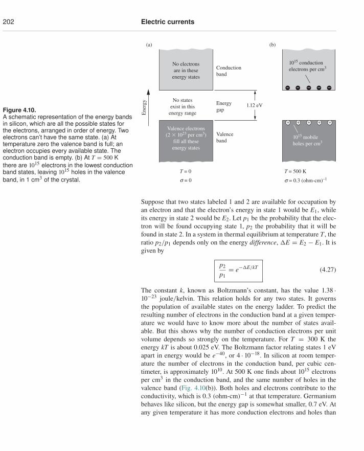
The above energy of 1.12 eV is the energy gap between two bands of pos-sible states, the valence band and the conduction band. States of inter-mediate energy for the electron simply do not exist. This energy ladder isrepresented in Fig. 4.10. Two electrons can never have the same quantumstate – that is a fundamental law of physics (the Pauli exclusion prin-ciple which you will learn about in quantum mechanics). States rangingup the energy ladder must therefore be occupied even at absolute zero.As it happens, there are exactly enough states in the valence band toaccommodate all the electrons. At T = 0, as shown in Fig. 4.10(a), allof these valence states are occupied, and none of the conduction bandstates is.
If the temperature is high enough, thermal energy can raise someelectrons from the valence band to the conduction band. The effect oftemperature on the probability that electron states will be occupied isexpressed by the exponential factor e−�E/kT , called the Boltzmann factor.
11 This mystery is not explained by drawing an analogy, as is sometimes done, with abubble in a liquid. In a centrifuge, bubbles in a liquid would go in toward the axis; theholes we are talking about would go out. A cryptic but true statement, which onlyquantum mechanics will make intelligible, is this: the hole behaves dynamically like apositive charge with positive mass because it is a vacancy in states with negativecharge and negative mass.
12 Technically, “eV” should be written as “eV,” because an electron-volt is the product oftwo things: the (magnitude of the) electron charge e and one volt V.
202 Electric currents
Figure 4.10.A schematic representation of the energy bandsin silicon, which are all the possible states forthe electrons, arranged in order of energy. Twoelectrons can’t have the same state. (a) Attemperature zero the valence band is full; anelectron occupies every available state. Theconduction band is empty. (b) At T = 500 Kthere are 1015 electrons in the lowest conductionband states, leaving 1015 holes in the valenceband, in 1 cm3 of the crystal.
1015 conductionelectrons per cm3Conduction
band
1.12 eVEnergygap
Valence electrons(2 � 1023 per cm3)
fill all theseenergy states
1015 mobileholes per cm3
T = 500 KT = 0
s = 0.3 (ohm-cm)–1s = 0
Valenceband
No statesexist in this
energy rangeEne
rgy
No electronsare in these
energy states
(a) (b)
+ + + + +
Suppose that two states labeled 1 and 2 are available for occupation byan electron and that the electron’s energy in state 1 would be E1, whileits energy in state 2 would be E2. Let p1 be the probability that the elec-tron will be found occupying state 1, p2 the probability that it will befound in state 2. In a system in thermal equilibrium at temperature T , theratio p2/p1 depends only on the energy difference, �E = E2 − E1. It isgiven by
p2
p1= e−�E/kT (4.27)
The constant k, known as Boltzmann’s constant, has the value 1.38 ·10−23 joule/kelvin. This relation holds for any two states. It governsthe population of available states on the energy ladder. To predict theresulting number of electrons in the conduction band at a given temper-ature we would have to know more about the number of states avail-able. But this shows why the number of conduction electrons per unitvolume depends so strongly on the temperature. For T = 300 K theenergy kT is about 0.025 eV. The Boltzmann factor relating states 1 eVapart in energy would be e−40, or 4 · 10−18. In silicon at room temper-ature the number of electrons in the conduction band, per cubic cen-timeter, is approximately 1010. At 500 K one finds about 1015 electronsper cm3 in the conduction band, and the same number of holes in thevalence band (Fig. 4.10(b)). Both holes and electrons contribute to theconductivity, which is 0.3 (ohm-cm)−1 at that temperature. Germaniumbehaves like silicon, but the energy gap is somewhat smaller, 0.7 eV. Atany given temperature it has more conduction electrons and holes than
4.6 Semiconductors 203
p-typesemiconductor
n-typesemiconductor
Electrons fromphosphorusimpurity atoms[5 � 1015 cm–3]
Holes left by electronsattaching to aluminumimpurity atoms[5 � 1015 cm–3]
Conductionband
Valenceband
(a) (b)
Electrons and holesas in pure silicon [1010 cm–3]
Electrons and holesas in pure silicon [1010 cm–3]
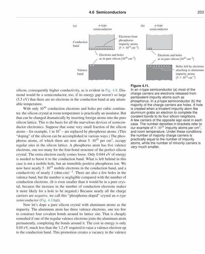
Figure 4.11.In an n-type semiconductor (a) most of thecharge carriers are electrons released frompentavalent impurity atoms such asphosphorus. In a p-type semiconductor (b) themajority of the charge carriers are holes. A holeis created when a trivalent impurity atom likealuminum grabs an electron to complete thecovalent bonds to its four silicon neighbors.A few carriers of the opposite sign exist in eachcase. The number densities in brackets refer toour example of 5 · 1015 impurity atoms per cm3,and room temperature. Under these conditionsthe number of majority charge carriers ispractically equal to the number of impurityatoms, while the number of minority carriers isvery much smaller.
silicon, consequently higher conductivity, as is evident in Fig. 4.8. Dia-mond would be a semiconductor, too, if its energy gap weren’t so large(5.5 eV) that there are no electrons in the conduction band at any attain-able temperature.
With only 1010 conduction electrons and holes per cubic centime-ter, the silicon crystal at room temperature is practically an insulator. Butthat can be changed dramatically by inserting foreign atoms into the puresilicon lattice. This is the basis for all the marvelous devices of semicon-ductor electronics. Suppose that some very small fraction of the siliconatoms – for example, 1 in 107 – are replaced by phosphorus atoms. (This“doping” of the silicon can be accomplished in various ways.) The phos-phorus atoms, of which there are now about 5 · 1015 per cm3, occupyregular sites in the silicon lattice. A phosphorus atom has five valenceelectrons, one too many for the four-bond structure of the perfect siliconcrystal. The extra electron easily comes loose. Only 0.044 eV of energyis needed to boost it to the conduction band. What is left behind in thiscase is not a mobile hole, but an immobile positive phosphorus ion. Wenow have nearly 5 · 1015 mobile electrons in the conduction band, and aconductivity of nearly 1 (ohm-cm)−1. There are also a few holes in thevalence band, but the number is negligible compared with the number ofconduction electrons. (It is even smaller than it would be in a pure crys-tal, because the increase in the number of conduction electrons makesit more likely for a hole to be negated.) Because nearly all the chargecarriers are negative, we call this “phosphorus-doped” crystal an n-typesemiconductor (Fig. 4.11(a)).
Now let’s dope a pure silicon crystal with aluminum atoms as theimpurity. The aluminum atom has three valence electrons, one too fewto construct four covalent bonds around its lattice site. That is cheaplyremedied if one of the regular valence electrons joins the aluminum atompermanently, completing the bonds around it. The cost in energy is only0.05 eV, much less than the 1.2 eV required to raise a valence electron upto the conduction band. This promotion creates a vacancy in the valence
204 Electric currents
band, a mobile hole, and turns the aluminum atom into a fixed negativeion. Thanks to the holes thus created – at room temperature nearly equalin number to the aluminum atoms added – the crystal becomes a muchbetter conductor. There are also a few electrons in the conduction band,but the overwhelming majority of the mobile charge carriers are positive,and we call this material a p-type semiconductor (Fig. 4.11(b)).
Once the number of mobile charge carriers has been established,whether electrons or holes or both, the conductivity depends on theirmobility, which is limited, as in metallic conduction, by scattering withinthe crystal. A single homogeneous semiconductor obeys Ohm’s law. Thespectacularly nonohmic behavior of semiconductor devices – as in a rec-tifier or a transistor – is achieved by combining n-type material withp-type material in various arrangements.
Example (Mean free time in silicon) In Fig. 4.10, a conductivity of30 (ohm-m)−1 results from the presence of 1021 electrons per m3 in the con-duction band, along with the same number of holes. Assume that τ+ = τ− andM+ = M− = me, the electron mass. What must be the value of the mean freetime τ? The rms speed of an electron at 500 K is 1.5 · 105 m/s. Compare themean free path with the distance between neighboring silicon atoms, which is2.35 · 10−10 m.
Solution Since we have two types of charge carriers, the electrons and theholes, Eq. (4.23) gives
τ = mσ
2Ne2 = (9.1 · 10−31 kg)(30 (ohm-m)−1)
2(1021 m−3)(1.6 · 10−19 C)2 ≈ 5.3 · 10−13 s. (4.28)
The distance traveled during this time is vτ = (1.5 · 105 m/s)(5.3 · 10−13 s) ≈8 · 10−8 m, which is more than 300 times the distance between neighboring sili-con atoms.
4.7 Circuits and circuit elementsElectrical devices usually have well-defined terminals to which wires canbe connected. Charge can flow into or out of the device over these paths.In particular, if two terminals, and only two, are connected by wires tosomething outside, and if the current flow is steady with constant poten-tials everywhere, then obviously the current must be equal and oppo-site at the two terminals.13 In that case we can speak of the current Ithat flows through the device, and of the voltage V “between the termi-nals” or “across the terminals,” which means their difference in electric
13 It is perfectly possible to have 4 A flowing into one terminal of a two-terminal objectwith 3 A flowing out at the other terminal. But then the object is accumulating positivecharge at the rate of 1 coulomb/second. Its potential must be changing very rapidly –and that can’t go on for long. Hence this cannot be a steady, or time-independent,current.
4.7 Circuits and circuit elements 205
potential. The ratio V/I for some given I is a certain number of resis-tance units (ohms, if V is in volts and I in amps). If Ohm’s law is obeyed
65 ohms
28 cm length of No. 40 nichrome wire
Two 70 ohm resistors and one 30 ohmresistor
25 watt 115 volt tungsten light bulb (cold)
0.5 N KCl solution with electrodes of certainsize and spacing
lb spool of No. 28 enameled copper magnet wire (1030 ft)
12
(a)
(b)
(c)
(d)
(e )
in all parts of the object through which current flows, that number willbe a constant, independent of the current. This one number completelydescribes the electrical behavior of the object, for steady current flow(DC) between the given terminals. With these rather obvious remarkswe introduce a simple idea, the notion of a circuit element.
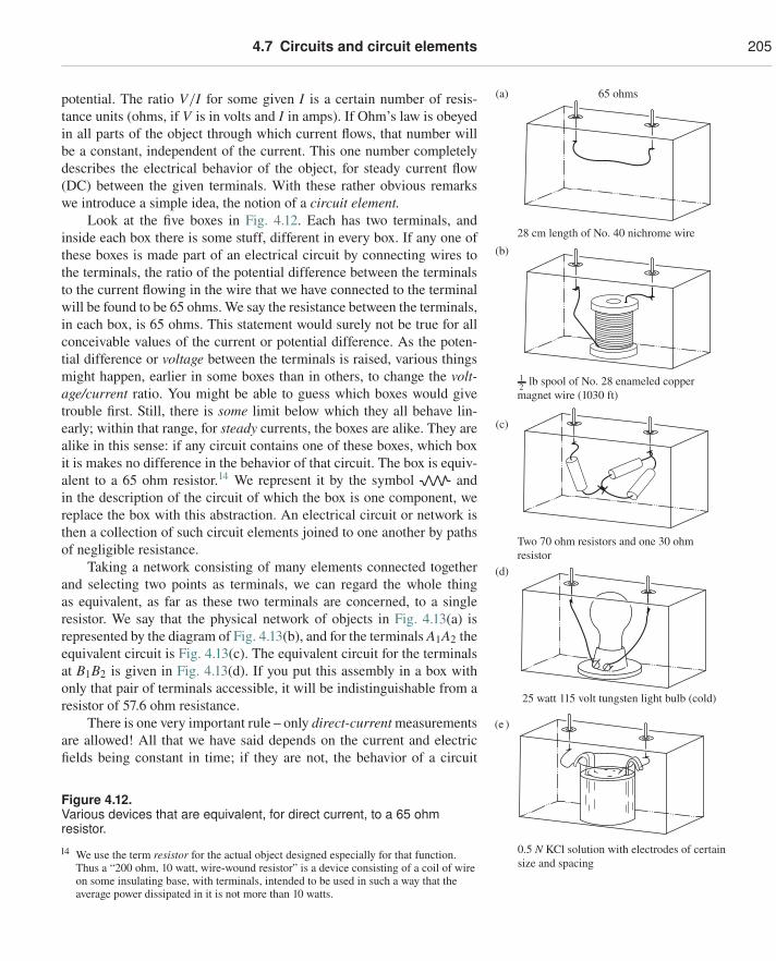
Look at the five boxes in Fig. 4.12. Each has two terminals, andinside each box there is some stuff, different in every box. If any one ofthese boxes is made part of an electrical circuit by connecting wires tothe terminals, the ratio of the potential difference between the terminalsto the current flowing in the wire that we have connected to the terminalwill be found to be 65 ohms. We say the resistance between the terminals,in each box, is 65 ohms. This statement would surely not be true for allconceivable values of the current or potential difference. As the poten-tial difference or voltage between the terminals is raised, various thingsmight happen, earlier in some boxes than in others, to change the volt-age/current ratio. You might be able to guess which boxes would givetrouble first. Still, there is some limit below which they all behave lin-early; within that range, for steady currents, the boxes are alike. They arealike in this sense: if any circuit contains one of these boxes, which boxit is makes no difference in the behavior of that circuit. The box is equiv-alent to a 65 ohm resistor.14 We represent it by the symbol andin the description of the circuit of which the box is one component, wereplace the box with this abstraction. An electrical circuit or network isthen a collection of such circuit elements joined to one another by pathsof negligible resistance.
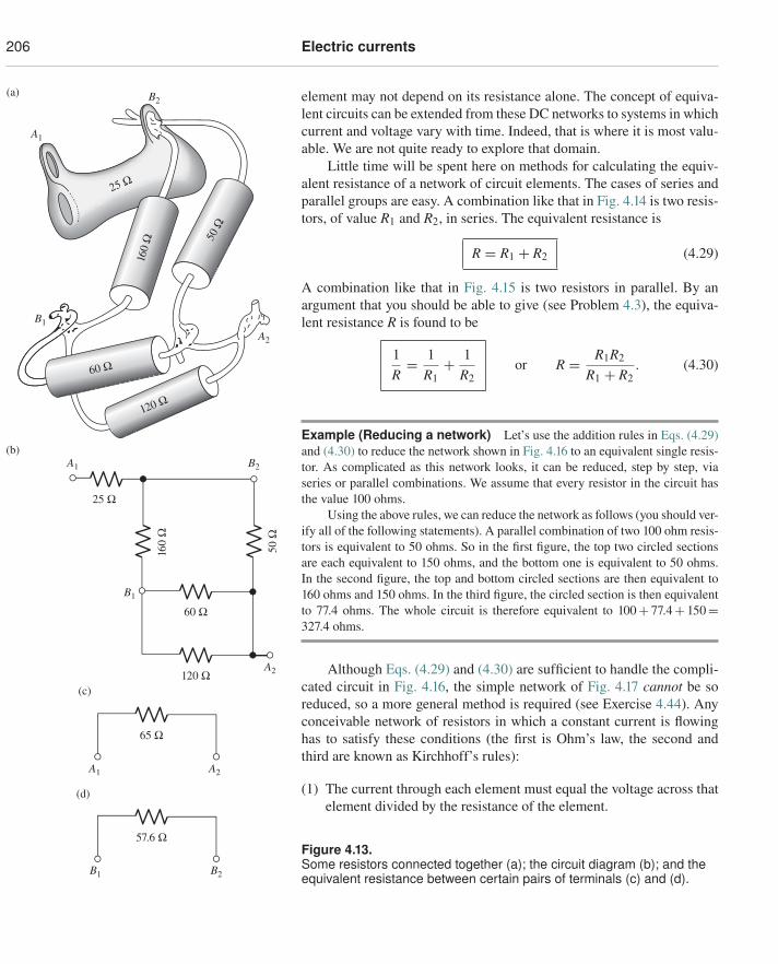
Taking a network consisting of many elements connected togetherand selecting two points as terminals, we can regard the whole thingas equivalent, as far as these two terminals are concerned, to a singleresistor. We say that the physical network of objects in Fig. 4.13(a) isrepresented by the diagram of Fig. 4.13(b), and for the terminals A1A2 theequivalent circuit is Fig. 4.13(c). The equivalent circuit for the terminalsat B1B2 is given in Fig. 4.13(d). If you put this assembly in a box withonly that pair of terminals accessible, it will be indistinguishable from aresistor of 57.6 ohm resistance.
There is one very important rule – only direct-current measurementsare allowed! All that we have said depends on the current and electricfields being constant in time; if they are not, the behavior of a circuit
Figure 4.12.Various devices that are equivalent, for direct current, to a 65 ohmresistor.
14 We use the term resistor for the actual object designed especially for that function.Thus a “200 ohm, 10 watt, wire-wound resistor” is a device consisting of a coil of wireon some insulating base, with terminals, intended to be used in such a way that theaverage power dissipated in it is not more than 10 watts.
206 Electric currents
element may not depend on its resistance alone. The concept of equiva-lent circuits can be extended from these DC networks to systems in which
A1
A2
25 Ω
160
Ω 50 Ω
60 Ω
120 Ω
B2
B1
(a)
(b)
(c)
(d)
A2
B2
B2
B1
A1
B1
A2A1
25 Ω
160
Ω
50 Ω
60 Ω
65 Ω
57.6 Ω
120 Ω
current and voltage vary with time. Indeed, that is where it is most valu-able. We are not quite ready to explore that domain.
Little time will be spent here on methods for calculating the equiv-alent resistance of a network of circuit elements. The cases of series andparallel groups are easy. A combination like that in Fig. 4.14 is two resis-tors, of value R1 and R2, in series. The equivalent resistance is
R = R1 + R2 (4.29)
A combination like that in Fig. 4.15 is two resistors in parallel. By anargument that you should be able to give (see Problem 4.3), the equiva-lent resistance R is found to be
1R= 1
R1+ 1
R2or R = R1R2
R1 + R2. (4.30)
Example (Reducing a network) Let’s use the addition rules in Eqs. (4.29)and (4.30) to reduce the network shown in Fig. 4.16 to an equivalent single resis-tor. As complicated as this network looks, it can be reduced, step by step, viaseries or parallel combinations. We assume that every resistor in the circuit hasthe value 100 ohms.
Using the above rules, we can reduce the network as follows (you should ver-ify all of the following statements). A parallel combination of two 100 ohm resis-tors is equivalent to 50 ohms. So in the first figure, the top two circled sectionsare each equivalent to 150 ohms, and the bottom one is equivalent to 50 ohms.In the second figure, the top and bottom circled sections are then equivalent to160 ohms and 150 ohms. In the third figure, the circled section is then equivalentto 77.4 ohms. The whole circuit is therefore equivalent to 100+ 77.4+ 150=327.4 ohms.
Although Eqs. (4.29) and (4.30) are sufficient to handle the compli-cated circuit in Fig. 4.16, the simple network of Fig. 4.17 cannot be soreduced, so a more general method is required (see Exercise 4.44). Anyconceivable network of resistors in which a constant current is flowinghas to satisfy these conditions (the first is Ohm’s law, the second andthird are known as Kirchhoff’s rules):
(1) The current through each element must equal the voltage across thatelement divided by the resistance of the element.
Figure 4.13.Some resistors connected together (a); the circuit diagram (b); and theequivalent resistance between certain pairs of terminals (c) and (d).
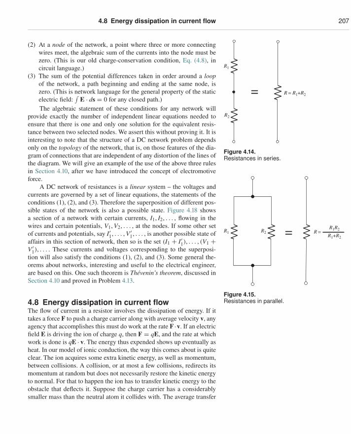
4.8 Energy dissipation in current flow 207
(2) At a node of the network, a point where three or more connectingwires meet, the algebraic sum of the currents into the node must be
R1
R = R1+R2
R2
=
Figure 4.14.Resistances in series.
zero. (This is our old charge-conservation condition, Eq. (4.8), incircuit language.)
(3) The sum of the potential differences taken in order around a loopof the network, a path beginning and ending at the same node, iszero. (This is network language for the general property of the staticelectric field:
∫E · ds = 0 for any closed path.)
The algebraic statement of these conditions for any network willprovide exactly the number of independent linear equations needed toensure that there is one and only one solution for the equivalent resis-tance between two selected nodes. We assert this without proving it. It isinteresting to note that the structure of a DC network problem dependsonly on the topology of the network, that is, on those features of the dia-gram of connections that are independent of any distortion of the lines ofthe diagram. We will give an example of the use of the above three rulesin Section 4.10, after we have introduced the concept of electromotiveforce.
A DC network of resistances is a linear system – the voltages andcurrents are governed by a set of linear equations, the statements of theconditions (1), (2), and (3). Therefore the superposition of different pos-sible states of the network is also a possible state. Figure 4.18 shows
R = =R1 R2R1R2
R1+R2
Figure 4.15.Resistances in parallel.
a section of a network with certain currents, I1, I2, . . . , flowing in thewires and certain potentials, V1, V2, . . . , at the nodes. If some other setof currents and potentials, say I′1, . . . , V ′
1, . . . , is another possible state ofaffairs in this section of network, then so is the set (I1 + I′1), . . . , (V1 +V ′
1), . . . . These currents and voltages corresponding to the superposi-tion will also satisfy the conditions (1), (2), and (3). Some general the-orems about networks, interesting and useful to the electrical engineer,are based on this. One such theorem is Thévenin’s theorem, discussed inSection 4.10 and proved in Problem 4.13.
4.8 Energy dissipation in current flowThe flow of current in a resistor involves the dissipation of energy. If ittakes a force F to push a charge carrier along with average velocity v, anyagency that accomplishes this must do work at the rate F ·v. If an electricfield E is driving the ion of charge q, then F = qE, and the rate at whichwork is done is qE · v. The energy thus expended shows up eventually asheat. In our model of ionic conduction, the way this comes about is quiteclear. The ion acquires some extra kinetic energy, as well as momentum,between collisions. A collision, or at most a few collisions, redirects itsmomentum at random but does not necessarily restore the kinetic energyto normal. For that to happen the ion has to transfer kinetic energy to theobstacle that deflects it. Suppose the charge carrier has a considerablysmaller mass than the neutral atom it collides with. The average transfer
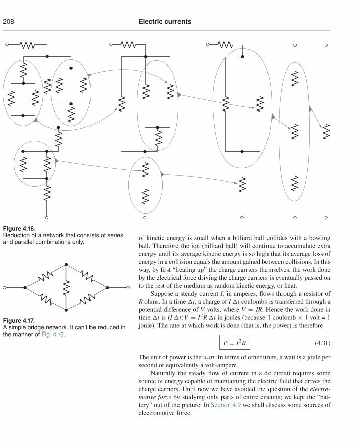
208 Electric currents
Figure 4.16.Reduction of a network that consists of seriesand parallel combinations only.
of kinetic energy is small when a billiard ball collides with a bowlingball. Therefore the ion (billiard ball) will continue to accumulate extraenergy until its average kinetic energy is so high that its average loss ofenergy in a collision equals the amount gained between collisions. In thisway, by first “heating up” the charge carriers themselves, the work doneby the electrical force driving the charge carriers is eventually passed onto the rest of the medium as random kinetic energy, or heat.
Figure 4.17.A simple bridge network. It can’t be reduced inthe manner of Fig. 4.16.
Suppose a steady current I, in amperes, flows through a resistor ofR ohms. In a time �t, a charge of I �t coulombs is transferred through apotential difference of V volts, where V = IR. Hence the work done intime �t is (I �t)V = I2R �t in joules (because 1 coulomb × 1 volt = 1joule). The rate at which work is done (that is, the power) is therefore
P = I2R (4.31)
The unit of power is the watt. In terms of other units, a watt is a joule persecond or equivalently a volt-ampere.
Naturally the steady flow of current in a dc circuit requires somesource of energy capable of maintaining the electric field that drives thecharge carriers. Until now we have avoided the question of the electro-motive force by studying only parts of entire circuits; we kept the “bat-tery” out of the picture. In Section 4.9 we shall discuss some sources ofelectromotive force.
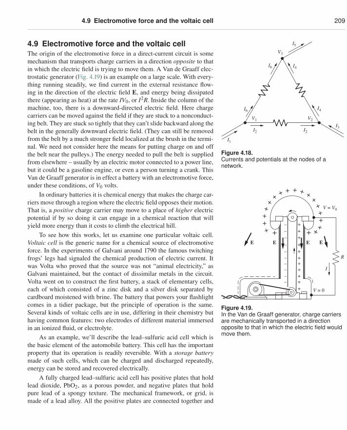
4.9 Electromotive force and the voltaic cell 209
4.9 Electromotive force and the voltaic cellThe origin of the electromotive force in a direct-current circuit is somemechanism that transports charge carriers in a direction opposite to that
I1
I2 I2I3
I4
I4
I5
V3
V1 V2
I6
I6
Figure 4.18.Currents and potentials at the nodes of anetwork.
in which the electric field is trying to move them. A Van de Graaff elec-trostatic generator (Fig. 4.19) is an example on a large scale. With every-thing running steadily, we find current in the external resistance flow-ing in the direction of the electric field E, and energy being dissipatedthere (appearing as heat) at the rate IV0, or I2R. Inside the column of themachine, too, there is a downward-directed electric field. Here chargecarriers can be moved against the field if they are stuck to a nonconduct-ing belt. They are stuck so tightly that they can’t slide backward along thebelt in the generally downward electric field. (They can still be removedfrom the belt by a much stronger field localized at the brush in the termi-nal. We need not consider here the means for putting charge on and offthe belt near the pulleys.) The energy needed to pull the belt is suppliedfrom elsewhere – usually by an electric motor connected to a power line,but it could be a gasoline engine, or even a person turning a crank. ThisVan de Graaff generator is in effect a battery with an electromotive force,under these conditions, of V0 volts.
In ordinary batteries it is chemical energy that makes the charge car-riers move through a region where the electric field opposes their motion.That is, a positive charge carrier may move to a place of higher electricpotential if by so doing it can engage in a chemical reaction that will
++
++
+
+ + + + + + ++
++
+
++++–
–––––––––
++++++++++
V = V0
V = 0
R
I
EEEE
Figure 4.19.In the Van de Graaff generator, charge carriersare mechanically transported in a directionopposite to that in which the electric field wouldmove them.
yield more energy than it costs to climb the electrical hill.To see how this works, let us examine one particular voltaic cell.
Voltaic cell is the generic name for a chemical source of electromotiveforce. In the experiments of Galvani around 1790 the famous twitchingfrogs’ legs had signaled the chemical production of electric current. Itwas Volta who proved that the source was not “animal electricity,” asGalvani maintained, but the contact of dissimilar metals in the circuit.Volta went on to construct the first battery, a stack of elementary cells,each of which consisted of a zinc disk and a silver disk separated bycardboard moistened with brine. The battery that powers your flashlightcomes in a tidier package, but the principle of operation is the same.Several kinds of voltaic cells are in use, differing in their chemistry buthaving common features: two electrodes of different material immersedin an ionized fluid, or electrolyte.
As an example, we’ll describe the lead–sulfuric acid cell which isthe basic element of the automobile battery. This cell has the importantproperty that its operation is readily reversible. With a storage batterymade of such cells, which can be charged and discharged repeatedly,energy can be stored and recovered electrically.
A fully charged lead–sulfuric acid cell has positive plates that holdlead dioxide, PbO2, as a porous powder, and negative plates that holdpure lead of a spongy texture. The mechanical framework, or grid, ismade of a lead alloy. All the positive plates are connected together and
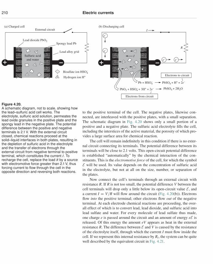
210 Electric currents
External circuit
+ –
Lead dioxide PbO2
Sulfuric acidand water
Spongy lead Pb
Lead alloy grid
Bisulfate ion HSO–4
Hydrogen ion H+
I
I
R
e–
e–
e– e–
(a) Charged cell (b) Discharging cell
Pb + HSO4–
PbO2 + HSO4– + 3H+ + 2e–
PbSO4 + H+ + 2e–
PbSO4 + 2H2O
–
+
–
–
–
– +
++
+
–– –
–
– +
+
+
+
+ –
Electrons from circuit
Electrons to circuit
Figure 4.20.A schematic diagram, not to scale, showing howthe lead–sulfuric acid cell works. Theelectrolyte, sulfuric acid solution, permeates thelead oxide granules in the positive plate and thespongy lead in the negative plate. The potentialdifference between the positive and negativeterminals is 2.1 V. With the external circuitclosed, chemical reactions proceed at thesolid–liquid interfaces in both plates, resulting inthe depletion of sulfuric acid in the electrolyteand the transfer of electrons through theexternal circuit from negative terminal to positiveterminal, which constitutes the current I. Torecharge the cell, replace the load R by a sourcewith electromotive force greater than 2.1 V, thusforcing current to flow through the cell in theopposite direction and reversing both reactions.
to the positive terminal of the cell. The negative plates, likewise con-nected, are interleaved with the positive plates, with a small separation.The schematic diagram in Fig. 4.20 shows only a small portion of apositive and a negative plate. The sulfuric acid electrolyte fills the cell,including the interstices of the active material, the porosity of which pro-vides a large surface area for chemical reaction.
The cell will remain indefinitely in this condition if there is no exter-nal circuit connecting its terminals. The potential difference between itsterminals will be close to 2.1 volts. This open-circuit potential differenceis established “automatically” by the chemical interaction of the con-stituents. This is the electromotive force of the cell, for which the symbolE will be used. Its value depends on the concentration of sulfuric acidin the electrolyte, but not at all on the size, number, or separation ofthe plates.
Now connect the cell’s terminals through an external circuit withresistance R. If R is not too small, the potential difference V between thecell terminals will drop only a little below its open-circuit value E , anda current I = V/R will flow around the circuit (Fig. 4.20(b)). Electronsflow into the positive terminal; other electrons flow out of the negativeterminal. At each electrode chemical reactions are proceeding, the over-all effect of which is to convert lead, lead dioxide, and sulfuric acid intolead sulfate and water. For every molecule of lead sulfate thus made,one charge e is passed around the circuit and an amount of energy eE isreleased. Of this energy the amount eV appears as heat in the externalresistance R. The difference between E and V is caused by the resistanceof the electrolyte itself, through which the current I must flow inside thecell. If we represent this internal resistance by Ri, the system can be quitewell described by the equivalent circuit in Fig. 4.21.
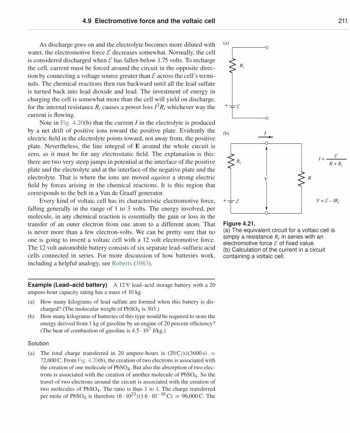
4.9 Electromotive force and the voltaic cell 211
As discharge goes on and the electrolyte becomes more diluted withwater, the electromotive force E decreases somewhat. Normally, the cellis considered discharged when E has fallen below 1.75 volts. To recharge
Ri
Ri R + Ri
R
I
I =
V = E – IRi
V
+
(a)
(b)
+
E
E
E
Figure 4.21.(a) The equivalent circuit for a voltaic cell issimply a resistance Ri in series with anelectromotive force E of fixed value.(b) Calculation of the current in a circuitcontaining a voltaic cell.
the cell, current must be forced around the circuit in the opposite direc-tion by connecting a voltage source greater than E across the cell’s termi-nals. The chemical reactions then run backward until all the lead sulfateis turned back into lead dioxide and lead. The investment of energy incharging the cell is somewhat more than the cell will yield on discharge,for the internal resistance Ri causes a power loss I2Ri whichever way thecurrent is flowing.
Note in Fig. 4.20(b) that the current I in the electrolyte is producedby a net drift of positive ions toward the positive plate. Evidently theelectric field in the electrolyte points toward, not away from, the positiveplate. Nevertheless, the line integral of E around the whole circuit iszero, as it must be for any electrostatic field. The explanation is this:there are two very steep jumps in potential at the interface of the positiveplate and the electrolyte and at the interface of the negative plate and theelectrolyte. That is where the ions are moved against a strong electricfield by forces arising in the chemical reactions. It is this region thatcorresponds to the belt in a Van de Graaff generator.
Every kind of voltaic cell has its characteristic electromotive force,falling generally in the range of 1 to 3 volts. The energy involved, permolecule, in any chemical reaction is essentially the gain or loss in thetransfer of an outer electron from one atom to a different atom. Thatis never more than a few electron-volts. We can be pretty sure that noone is going to invent a voltaic cell with a 12 volt electromotive force.The 12 volt automobile battery consists of six separate lead–sulfuric acidcells connected in series. For more discussion of how batteries work,including a helpful analogy, see Roberts (1983).
Example (Lead–acid battery) A 12 V lead–acid storage battery with a 20ampere-hour capacity rating has a mass of 10 kg.
(a) How many kilograms of lead sulfate are formed when this battery is dis-charged? (The molecular weight of PbSO4 is 303.)
(b) How many kilograms of batteries of this type would be required to store theenergy derived from 1 kg of gasoline by an engine of 20 percent efficiency?(The heat of combustion of gasoline is 4.5 · 107 J/kg.)
Solution
(a) The total charge transferred in 20 ampere-hours is (20 C/s)(3600 s) =72,000 C. From Fig. 4.20(b), the creation of two electrons is associated withthe creation of one molecule of PbSO4. But also the absorption of two elec-trons is associated with the creation of another molecule of PbSO4. So thetravel of two electrons around the circuit is associated with the creation oftwo molecules of PbSO4. The ratio is thus 1 to 1. The charge transferredper mole of PbSO4 is therefore (6 · 1023)(1.6 · 10−19 C) = 96,000 C. The
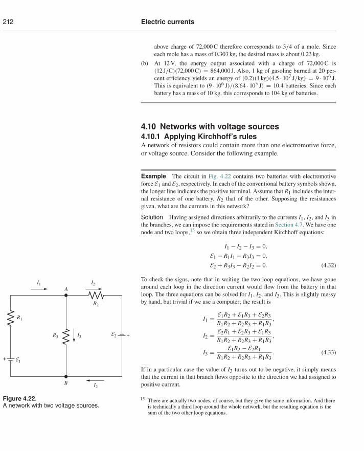
212 Electric currents
above charge of 72,000 C therefore corresponds to 3/4 of a mole. Sinceeach mole has a mass of 0.303 kg, the desired mass is about 0.23 kg.
(b) At 12 V, the energy output associated with a charge of 72,000 C is(12 J/C)(72,000 C) = 864,000 J. Also, 1 kg of gasoline burned at 20 per-cent efficiency yields an energy of (0.2)(1 kg)(4.5 · 107 J/kg) = 9 · 106 J.This is equivalent to (9 · 106 J)/(8.64 · 105 J) = 10.4 batteries. Since eachbattery has a mass of 10 kg, this corresponds to 104 kg of batteries.
4.10 Networks with voltage sources4.10.1 Applying Kirchhoff’s rulesA network of resistors could contain more than one electromotive force,or voltage source. Consider the following example.
Example The circuit in Fig. 4.22 contains two batteries with electromotive
I1A
B
I3
I2
I2
R2
R1
R3
E1
E2
+
+
Figure 4.22.A network with two voltage sources.
force E1 and E2, respectively. In each of the conventional battery symbols shown,the longer line indicates the positive terminal. Assume that R1 includes the inter-nal resistance of one battery, R2 that of the other. Supposing the resistancesgiven, what are the currents in this network?
Solution Having assigned directions arbitrarily to the currents I1, I2, and I3 inthe branches, we can impose the requirements stated in Section 4.7. We have onenode and two loops,15 so we obtain three independent Kirchhoff equations:
I1 − I2 − I3 = 0,
E1 − R1I1 − R3I3 = 0,
E2 + R3I3 − R2I2 = 0. (4.32)
To check the signs, note that in writing the two loop equations, we have gonearound each loop in the direction current would flow from the battery in thatloop. The three equations can be solved for I1, I2, and I3. This is slightly messyby hand, but trivial if we use a computer; the result is
I1 = E1R2 + E1R3 + E2R3R1R2 + R2R3 + R1R3
,
I2 = E2R1 + E2R3 + E1R3R1R2 + R2R3 + R1R3
,
I3 = E1R2 − E2R1R1R2 + R2R3 + R1R3
. (4.33)
If in a particular case the value of I3 turns out to be negative, it simply meansthat the current in that branch flows opposite to the direction we had assigned topositive current.
15 There are actually two nodes, of course, but they give the same information. And thereis technically a third loop around the whole network, but the resulting equation is thesum of the two other loop equations.
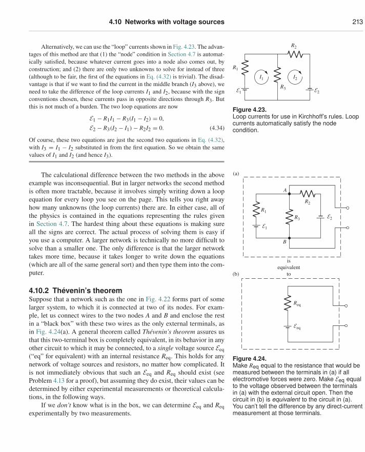
4.10 Networks with voltage sources 213
Alternatively, we can use the “loop” currents shown in Fig. 4.23. The advan-tages of this method are that (1) the “node” condition in Section 4.7 is automat-ically satisfied, because whatever current goes into a node also comes out, by
R1
E1 E2
R2
R3
I1 I2
Figure 4.23.Loop currents for use in Kirchhoff’s rules. Loopcurrents automatically satisfy the nodecondition.
construction; and (2) there are only two unknowns to solve for instead of three(although to be fair, the first of the equations in Eq. (4.32) is trivial). The disad-vantage is that if we want to find the current in the middle branch (I3 above), weneed to take the difference of the loop currents I1 and I2, because with the signconventions chosen, these currents pass in opposite directions through R3. Butthis is not much of a burden. The two loop equations are now
E1 − R1I1 − R3(I1 − I2) = 0,
E2 − R3(I2 − I1) − R2I2 = 0. (4.34)
Of course, these two equations are just the second two equations in Eq. (4.32),with I3 = I1 − I2 substituted in from the first equation. So we obtain the samevalues of I1 and I2 (and hence I3).
R2
A
R3
Req
Eeq
B
R1
E1
E2
isequivalent
to
(a)
(b)
Figure 4.24.Make Req equal to the resistance that would bemeasured between the terminals in (a) if allelectromotive forces were zero. Make Eeq equalto the voltage observed between the terminalsin (a) with the external circuit open. Then thecircuit in (b) is equivalent to the circuit in (a).You can’t tell the difference by any direct-currentmeasurement at those terminals.
The calculational difference between the two methods in the aboveexample was inconsequential. But in larger networks the second methodis often more tractable, because it involves simply writing down a loopequation for every loop you see on the page. This tells you right awayhow many unknowns (the loop currents) there are. In either case, all ofthe physics is contained in the equations representing the rules givenin Section 4.7. The hardest thing about these equations is making sureall the signs are correct. The actual process of solving them is easy ifyou use a computer. A larger network is technically no more difficult tosolve than a smaller one. The only difference is that the larger networktakes more time, because it takes longer to write down the equations(which are all of the same general sort) and then type them into the com-puter.
4.10.2 Thévenin’s theoremSuppose that a network such as the one in Fig. 4.22 forms part of somelarger system, to which it is connected at two of its nodes. For exam-ple, let us connect wires to the two nodes A and B and enclose the restin a “black box” with these two wires as the only external terminals, asin Fig. 4.24(a). A general theorem called Thévenin’s theorem assures usthat this two-terminal box is completely equivalent, in its behavior in anyother circuit to which it may be connected, to a single voltage source Eeq(“eq” for equivalent) with an internal resistance Req. This holds for anynetwork of voltage sources and resistors, no matter how complicated. Itis not immediately obvious that such an Eeq and Req should exist (seeProblem 4.13 for a proof), but assuming they do exist, their values can bedetermined by either experimental measurements or theoretical calcula-tions, in the following ways.
If we don’t know what is in the box, we can determine Eeq and Reqexperimentally by two measurements.
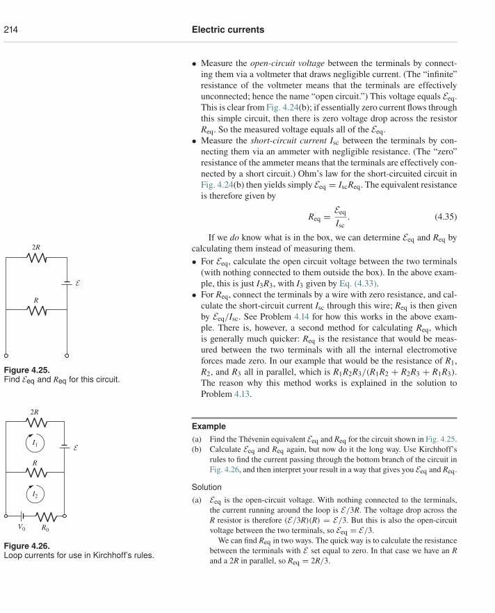
214 Electric currents
• Measure the open-circuit voltage between the terminals by connect-ing them via a voltmeter that draws negligible current. (The “infinite”resistance of the voltmeter means that the terminals are effectivelyunconnected; hence the name “open circuit.”) This voltage equals Eeq.This is clear from Fig. 4.24(b); if essentially zero current flows throughthis simple circuit, then there is zero voltage drop across the resistorReq. So the measured voltage equals all of the Eeq.
• Measure the short-circuit current Isc between the terminals by con-necting them via an ammeter with negligible resistance. (The “zero”resistance of the ammeter means that the terminals are effectively con-nected by a short circuit.) Ohm’s law for the short-circuited circuit inFig. 4.24(b) then yields simply Eeq = IscReq. The equivalent resistanceis therefore given by
Req = Eeq
Isc. (4.35)
If we do know what is in the box, we can determine Eeq and Req bycalculating them instead of measuring them.• For Eeq, calculate the open circuit voltage between the two terminals
R
2R
E
Figure 4.25.Find Eeq and Req for this circuit.
(with nothing connected to them outside the box). In the above exam-ple, this is just I3R3, with I3 given by Eq. (4.33).
• For Req, connect the terminals by a wire with zero resistance, and cal-culate the short-circuit current Isc through this wire; Req is then givenby Eeq/Isc. See Problem 4.14 for how this works in the above exam-ple. There is, however, a second method for calculating Req, whichis generally much quicker: Req is the resistance that would be meas-ured between the two terminals with all the internal electromotiveforces made zero. In our example that would be the resistance of R1,R2, and R3 all in parallel, which is R1R2R3/(R1R2 + R2R3 + R1R3).The reason why this method works is explained in the solution toProblem 4.13.
Example(a) Find the Thévenin equivalent Eeq and Req for the circuit shown in Fig. 4.25.
R0V0
R
2R
I1
I2
E
Figure 4.26.Loop currents for use in Kirchhoff’s rules.
(b) Calculate Eeq and Req again, but now do it the long way. Use Kirchhoff’srules to find the current passing through the bottom branch of the circuit inFig. 4.26, and then interpret your result in a way that gives you Eeq and Req.
Solution(a) Eeq is the open-circuit voltage. With nothing connected to the terminals,
the current running around the loop is E/3R. The voltage drop across theR resistor is therefore (E/3R)(R) = E/3. But this is also the open-circuitvoltage between the two terminals, so Eeq = E/3.
We can find Req in two ways. The quick way is to calculate the resistancebetween the terminals with E set equal to zero. In that case we have an Rand a 2R in parallel, so Req = 2R/3.
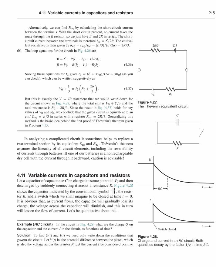
4.11 Variable currents in capacitors and resistors 215
Alternatively, we can find Req by calculating the short-circuit currentbetween the terminals. With the short circuit present, no current takes theroute through the R resistor, so we just have E and 2R in series. The short-circuit current between the terminals is therefore Isc = E/2R. The equiva-lent resistance is then given by Req = Eeq/Isc = (E/3)/(E/2R) = 2R/3.
(b) The loop equations for the circuit in Fig. 4.26 are
0 = E − R(I1 − I2) − (2R)I1,
0 = V0 − R(I2 − I1) − R0I2. (4.36)
2R/3
R0V0
E/3
Figure 4.27.The Thévenin equivalent circuit.
Solving these equations for I2 gives I2 = (E + 3V0)/(2R + 3R0) (as youcan check), which can be written suggestively as
V0 + E3= I2
(R0 + 2R
3
). (4.37)
But this is exactly the V = IR statement that we would write down forthe circuit shown in Fig. 4.27, where the total emf is V0 + E/3 and thetotal resistance is R0 + 2R/3. Since the result in Eq. (4.37) holds for anyvalues of V0 and R0, we conclude that the given circuit is equivalent to anemf Eeq = E/3 in series with a resistor Req = 2R/3. Generalizing thismethod is the basic idea behind the first proof of Thévenin’s theorem givenin Problem 4.13.
C
R
Q
I
t
t
RC
Switch closed
Figure 4.28.Charge and current in an RC circuit. Bothquantities decay by the factor 1/e in time RC.
In analyzing a complicated circuit it sometimes helps to replace atwo-terminal section by its equivalent Eeq and Req. Thévenin’s theoremassumes the linearity of all circuit elements, including the reversibilityof currents through batteries. If one of our batteries is a nonrechargeabledry cell with the current through it backward, caution is advisable!
4.11 Variable currents in capacitors and resistorsLet a capacitor of capacitance C be charged to some potential V0 and thendischarged by suddenly connecting it across a resistance R. Figure 4.28shows the capacitor indicated by the conventional symbol , the resis-tor R, and a switch which we shall imagine to be closed at time t = 0.It is obvious that, as current flows, the capacitor will gradually lose itscharge, the voltage across the capacitor will diminish, and this in turnwill lessen the flow of current. Let’s be quantitative about this.
Example (RC circuit) In the circuit in Fig. 4.28, what are the charge Q onthe capacitor and the current I in the circuit, as functions of time?
Solution To find Q(t) and I(t) we need only write down the conditions thatgovern the circuit. Let V(t) be the potential difference between the plates, whichis also the voltage across the resistor R. Let the current I be considered positive
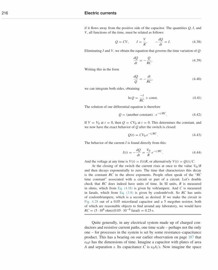
216 Electric currents
if it flows away from the positive side of the capacitor. The quantities Q, I, andV , all functions of the time, must be related as follows:
Q = CV , I = VR
, −dQdt
= I. (4.38)
Eliminating I and V , we obtain the equation that governs the time variation of Q:
dQdt
= − QRC
. (4.39)
Writing this in the form
dQQ
= − dtRC
, (4.40)
we can integrate both sides, obtaining
ln Q = −tRC
+ const. (4.41)
The solution of our differential equation is therefore
Q = (another constant) · e−t/RC . (4.42)
If V = V0 at t = 0, then Q = CV0 at t = 0. This determines the constant, andwe now have the exact behavior of Q after the switch is closed:
Q(t) = CV0 e−t/RC . (4.43)
The behavior of the current I is found directly from this:
I(t) = −dQdt
= V0R
e−t/RC . (4.44)
And the voltage at any time is V(t) = I(t)R, or alternatively V(t) = Q(t)/C.At the closing of the switch the current rises at once to the value V0/R
and then decays exponentially to zero. The time that characterizes this decayis the constant RC in the above exponents. People often speak of the “RCtime constant” associated with a circuit or part of a circuit. Let’s doublecheck that RC does indeed have units of time. In SI units, R is measuredin ohms, which from Eq. (4.18) is given by volt/ampere. And C is measuredin farads, which from Eq. (3.8) is given by coulomb/volt. So RC has unitsof coulomb/ampere, which is a second, as desired. If we make the circuit inFig. 4.28 out of a 0.05 microfarad capacitor and a 5 megohm resistor, bothof which are reasonable objects to find around any laboratory, we would haveRC = (5 · 106 ohm)(0.05 · 10−6 farad) = 0.25 s.
Quite generally, in any electrical system made up of charged con-ductors and resistive current paths, one time scale – perhaps not the onlyone – for processes in the system is set by some resistance–capacitanceproduct. This has a bearing on our earlier observation on page 187 thatε0ρ has the dimensions of time. Imagine a capacitor with plates of areaA and separation s. Its capacitance C is ε0A/s. Now imagine the space
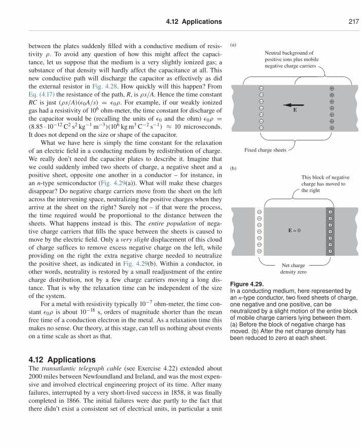
4.12 Applications 217
between the plates suddenly filled with a conductive medium of resis-tivity ρ. To avoid any question of how this might affect the capaci-tance, let us suppose that the medium is a very slightly ionized gas; asubstance of that density will hardly affect the capacitance at all. Thisnew conductive path will discharge the capacitor as effectively as didthe external resistor in Fig. 4.28. How quickly will this happen? FromEq. (4.17) the resistance of the path, R, is ρs/A. Hence the time constantRC is just (ρs/A)(ε0A/s) = ε0ρ. For example, if our weakly ionizedgas had a resistivity of 106 ohm-meter, the time constant for discharge ofthe capacitor would be (recalling the units of ε0 and the ohm) ε0ρ =
Neutral background ofpositive ions plus mobilenegative charge carriers
Fixed charge sheets
⊕⊕⊕⊕⊕⊕⊕
(a)
(b)
E
E = 0
This block of negativecharge has moved tothe right
Net chargedensity zero
Figure 4.29.In a conducting medium, here represented byan n-type conductor, two fixed sheets of charge,one negative and one positive, can beneutralized by a slight motion of the entire blockof mobile charge carriers lying between them.(a) Before the block of negative charge hasmoved. (b) After the net charge density hasbeen reduced to zero at each sheet.
(8.85 · 10−12 C2 s2 kg−1 m−3)(106 kg m3 C−2 s−1) ≈ 10 microseconds.It does not depend on the size or shape of the capacitor.
What we have here is simply the time constant for the relaxationof an electric field in a conducting medium by redistribution of charge.We really don’t need the capacitor plates to describe it. Imagine thatwe could suddenly imbed two sheets of charge, a negative sheet and apositive sheet, opposite one another in a conductor – for instance, inan n-type semiconductor (Fig. 4.29(a)). What will make these chargesdisappear? Do negative charge carriers move from the sheet on the leftacross the intervening space, neutralizing the positive charges when theyarrive at the sheet on the right? Surely not – if that were the process,the time required would be proportional to the distance between thesheets. What happens instead is this. The entire population of nega-tive charge carriers that fills the space between the sheets is caused tomove by the electric field. Only a very slight displacement of this cloudof charge suffices to remove excess negative charge on the left, whileproviding on the right the extra negative charge needed to neutralizethe positive sheet, as indicated in Fig. 4.29(b). Within a conductor, inother words, neutrality is restored by a small readjustment of the entirecharge distribution, not by a few charge carriers moving a long dis-tance. That is why the relaxation time can be independent of the sizeof the system.
For a metal with resistivity typically 10−7 ohm-meter, the time con-stant ε0ρ is about 10−18 s, orders of magnitude shorter than the meanfree time of a conduction electron in the metal. As a relaxation time thismakes no sense. Our theory, at this stage, can tell us nothing about eventson a time scale as short as that.
4.12 ApplicationsThe transatlantic telegraph cable (see Exercise 4.22) extended about2000 miles between Newfoundland and Ireland, and was the most expen-sive and involved electrical engineering project of its time. After manyfailures, interrupted by a very short-lived success in 1858, it was finallycompleted in 1866. The initial failures were due partly to the fact thatthere didn’t exist a consistent set of electrical units, in particular a unit
218 Electric currents
for resistance. A byproduct of the project was therefore the hastening ofa consistent set of units.
Electric shocks can range from barely noticeable, to annoying, topainful, to lethal. The severity of a shock depends on the current, not theapplied voltage (although for a given resistance, a higher voltage meansa higher current, of course). The duration also matters. The current canbe harmful for two reasons: it can cause burns, and it can cause the heartto undergo fibrillation, where the normal coordinated contractions arereplaced by uncoordinated ones, which don’t pump any blood. Currentsas small as 50 mA can cause fibrillation. A defibrillator works by passinga large enough current through the heart so that it briefly freezes up.With the uncoordinated contractions halted, the heart is then likely tostart beating normally.
A current of 10 mA running through your hand is roughly the “can’tlet go” threshold, where the induced contractions of the muscles preventyou from letting go of the wire or whatever the voltage source is. And ifyou can’t let go, you will inevitably become sweaty, which will reducethe resistivity of your skin, making things even worse. People who workwith electricity often keep one hand in their pocket, to reduce the chanceof it touching a grounded object and forming a conductive path, and,even worse, a path that goes across the heart.
If you touch a voltage source, the relation between the voltage andcurrent depends on the resistance involved, and this can vary greatly,depending on the conditions. The main things that the resistance dependson are the resistivity of your skin, and the contact area. Dry skin hasa much higher resistivity than wet skin. In a given scenario, the dry-skin resistance might be, say, 100,000 �, whereas the wet-skin resistancemight be 1000 �. The shock from a 120 V wall socket in these two caseswill be about 1 mA (hardly noticeable), or about 100 mA (potentiallylethal). It’s best to assume the latter! The variation of resistivity with thesweatiness of your skin is one of the ingredients in lie-detector machines.The increase in current is quite remarkable, even if you don’t think you’resweating much. If you hook yourself up to an apparatus of this sort(which can often be found in science museums and the like), and if youthen imagine, say, bungee jumping off a high suspension bridge, the cur-rent will rise dramatically. It’s like it is magically reading your mind. Thewet interior of our bodies has an even lower resistivity, of course, so spe-cial precautions must be taken in hospital operating rooms. Even a smallvoltage across an exposed heart can create a sufficient current to causefibrillation.
If you shuffle your feet across a carpet on a dry day, you can getcharged up to a very high voltage, perhaps 50,000 V. If you then toucha grounded object, you get a shock in the form of a spark. But evenif you’re quite sweaty, this 50,000 V certainly isn’t lethal, whereas the120 V from the wall socket might very well be. As mentioned in Section2.18, the reason is that the amount of charge on you after shuffling across
4.12 Applications 219
the carpet is very small, whereas there is an essentially infinite amountof charge available from the power company. The current in the case ofthe carpet lasts for a very short time before the charge runs out, and thistime interval is too short to do any damage.
A fuse is a safety device that protects against large currents in acircuit; 20 A is a typical threshold. Such currents can generate enoughheat to start a fire. A fuse consists of a thin strip of metal connected inseries with the circuit. If the current becomes sufficiently large, the I2Rresistance heating will melt the strip, producing a gap in the circuit andhalting the current flow. A fuse needs to be replaced each time it burnsout, but it’s better to burn out a fuse than to burn down a house! A similarsafety device, a circuit breaker, doesn’t need to be replaced; it can simplybe reset. This will be discussed in Section 6.10.
A smoke detector of the “ionization” type works by monitoring atiny current. This current is created by a small radioactive source thatemits alpha particles, which ionize the air. These ions constitute the tinycurrent. When smoke enters the detector, the ions collect on the smokeparticles and are neutralized. This disrupts the current, telling the alarmto go off.
Electric eels can generate voltages on the order of 500 V, which isenough to harm or possibly kill a human. The discharge is brief; a currentof about 1 ampere lasts for a few milliseconds, but this is long enough.Special electrocyte cells, which take up most of the eel’s body, are able togenerate small voltages of roughly 0.1 V by means of sodium–potassiumpumps (a common mechanism in nerve and muscle cells). Thousands ofthese cells are stacked in series (the same basic idea behind a battery) toproduce the 500 V potential, and then many of these stacks are combinedin parallel. The tricky thing is for the eel to discharge all the electrocytecells simultaneously; the mechanism for this isn’t entirely understood.
Sprites are faint flashes of light that sometimes occur high abovethunderstorms. They are predominantly red and generally extend verti-cally, sometimes up to 100 km. There are still many open questions abouthow they form, but an important fact is that the air is much less denseat high altitudes, so the breakdown field is lower. (Electrons have moretime to accelerate between collisions, so they can achieve larger speeds.)A relatively small field, caused by a dipole distribution of charge in athundercloud, can be large enough at high altitudes to cause breakdown.
In a conducting metal wire, current can flow in either direction. Thetwo directions are symmetrical; if you flip the wire over, it looks thesame. But in a diode, current can flow in only one direction. A semi-conductor diode consists of an n-type semiconducting region adjacent toa p-type region (the combination is called a p-n junction). The currentsin these regions arise from the flow of electrons and holes, respectively.Because of this difference, there is an asymmetry between the two direc-tions of current flow. This setup therefore has at least some chance ofallowing current to flow in only one direction. And indeed, it can be
220 Electric currents
shown that (provided that the voltage isn’t excessively large) current canflow only in the p-to-n direction. Or, equivalently, electrons can flow onlyin the n-to-p direction. The reasoning involves the diffusion of electronsand holes across the junction, which creates a depletion region, wherethere are no mobile charge carriers. Alternatively, electrons can’t flowfrom the p region to the n region, because there are no mobile electronsin the p region to do the flowing.
When a current flows through a diode, electrons give off energy bydropping from the conduction band down to a hole in the valence band.This energy takes the form of a photon, and for certain materials theenergy gap corresponds to a photon whose frequency is in the visiblespectrum. Such a diode is called a light-emitting diode (LED). LEDs lastmuch longer than incandescent bulbs (there is no filament that will burnout), and they are much more energy efficient (there is less wasted heat,and fewer wasted photons in nonvisible parts of the spectrum). They arealso generally very small, so they can easily be inserted into circuits.
A transistor is a device that allows a small signal in one part of acircuit to control a large current in another part. A transistor can be madewith, for example, an n-p-n junction (although the middle region mustbe very thin for it to work). This is called a bipolar junction transistor(BJT). If two terminals are connected to the two n-type materials on theends, no current will flow through the transistor, because it effectivelyconsists of two p-n junctions pointing in opposite directions, But if asmall current is allowed to flow through the middle p-type material byway of a third terminal, then it turns out (although this is by no meansobvious) that a much larger current will flow through the transistor, thatis, through the original two terminals. A transistor can operate in an “allor nothing” mode, that is, as a switch that turns a large current on oroff. Or it can operate in a continuous manner, where the resultant currentdepends on the small current in the middle p-type material.
Another type of transistor is the field effect transistor (FET). Thereare different types of FETs, but in one type a gate runs along the sideof a p-type material. If a positive voltage is applied to the gate, it willattract electrons and effectively turn a thin layer of the p-type materialinto n-type. If terminals are connected to two n-type regions that areplaced at the ends of this layer, then we have a continuous n-type regionrunning from one terminal to the other, so current can flow. Increas-ing the gate voltage increases the thickness of the n-type layer, therebyincreasing the current flow between the terminals. The result is an ampli-fication of the original signal to the gate. And indeed, the transistor is themain component in the amplifier in your sound system. Although BJTswere developed first, FETs are by far the dominant transistor in modernelectronics.
Solar cells produce power by making use of the photovoltaic effect.At a p-n junction of two semiconducting materials, an electric field nat-urally occurs (see Exercise 4.26) due to the diffusion of electrons from
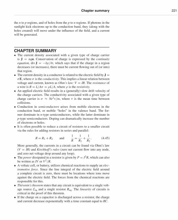
Chapter summary 221
the n to p regions, and of holes from the p to n regions. If photons in thesunlight kick electrons up to the conduction band, they (along with theholes created) will move under the influence of the field, and a currentwill be generated.
CHAPTER SUMMARY• The current density associated with a given type of charge carrier
is J = nqu. Conservation of charge is expressed by the continuityequation, div J = −∂ρ/∂t, which says that if the charge in a regiondecreases (or increases), there must be current flowing out of (or into)that region.
• The current density in a conductor is related to the electric field by J =σE, where σ is the conductivity. This implies a linear relation betweenvoltage and current, known as Ohm’s law: V = IR. The resistance ofa wire is R = L/Aσ = ρL/A, where ρ is the resistivity.
• An applied electric field results in a (generally) slow drift velocity ofthe charge carriers. The conductivity associated with a given type ofcharge carrier is σ ≈ Ne2τ/m, where τ is the mean time betweencollisions.
• Conduction in semiconductors arises from mobile electrons in theconduction band, or mobile “holes” in the valence band. The for-mer dominate in n-type semiconductors, while the latter dominate inp-type semiconductors. Doping can dramatically increase the numberof electrons or holes.
• It is often possible to reduce a circuit of resistors to a smaller circuitvia the rules for adding resistors in series and parallel:
R = R1 + R2 and1R= 1
R1+ 1
R2. (4.45)
More generally, the currents in a circuit can be found via Ohm’s law(V = IR) and Kirchhoff’s rules (zero net current flow into any node,and zero net voltage drop around any loop).
• The power dissipated in a resistor is given by P = I2R, which can alsobe written as IV or V2/R.
• A voltaic cell, or battery, utilizes chemical reactions to supply an elec-tromotive force. Since the line integral of the electric field arounda complete circuit is zero, there must be locations where ions moveagainst the electric field. The forces from the chemical reactions areresponsible for this.
• Thévenin’s theorem states that any circuit is equivalent to a single volt-age source Eeq and a single resistor Req. The linearity of circuits iscritical in the proof of this theorem.
• If the charge on a capacitor is discharged across a resistor, the chargeand current decrease exponentially with a time constant equal to RC.
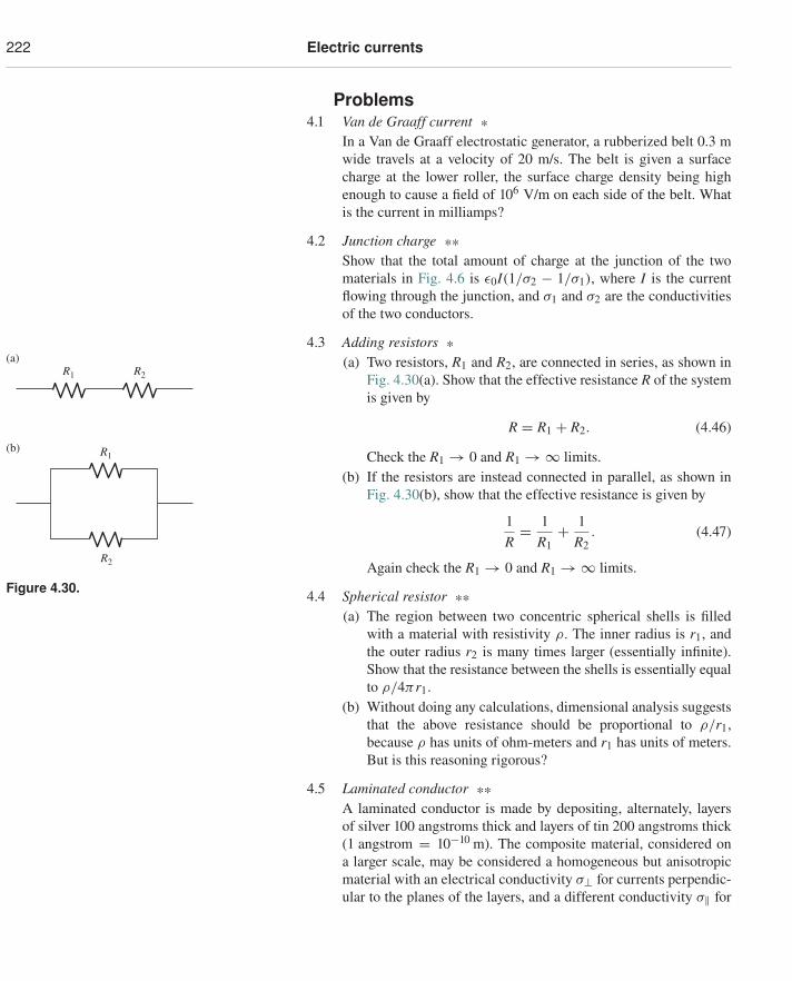
222 Electric currents
Problems4.1 Van de Graaff current *
In a Van de Graaff electrostatic generator, a rubberized belt 0.3 mwide travels at a velocity of 20 m/s. The belt is given a surfacecharge at the lower roller, the surface charge density being highenough to cause a field of 106 V/m on each side of the belt. Whatis the current in milliamps?
4.2 Junction charge **Show that the total amount of charge at the junction of the twomaterials in Fig. 4.6 is ε0I(1/σ2 − 1/σ1), where I is the currentflowing through the junction, and σ1 and σ2 are the conductivitiesof the two conductors.
4.3 Adding resistors *(a) Two resistors, R1 and R2, are connected in series, as shown in
Fig. 4.30(a). Show that the effective resistance R of the system
(a)
(b)
R1
R1
R2
R2
Figure 4.30.
is given by
R = R1 + R2. (4.46)
Check the R1 → 0 and R1 → ∞ limits.(b) If the resistors are instead connected in parallel, as shown in
Fig. 4.30(b), show that the effective resistance is given by
1R= 1
R1+ 1
R2. (4.47)
Again check the R1 → 0 and R1 → ∞ limits.
4.4 Spherical resistor **(a) The region between two concentric spherical shells is filled
with a material with resistivity ρ. The inner radius is r1, andthe outer radius r2 is many times larger (essentially infinite).Show that the resistance between the shells is essentially equalto ρ/4πr1.
(b) Without doing any calculations, dimensional analysis suggeststhat the above resistance should be proportional to ρ/r1,because ρ has units of ohm-meters and r1 has units of meters.But is this reasoning rigorous?
4.5 Laminated conductor **A laminated conductor is made by depositing, alternately, layersof silver 100 angstroms thick and layers of tin 200 angstroms thick(1 angstrom = 10−10 m). The composite material, considered ona larger scale, may be considered a homogeneous but anisotropicmaterial with an electrical conductivity σ⊥ for currents perpendic-ular to the planes of the layers, and a different conductivity σ‖ for
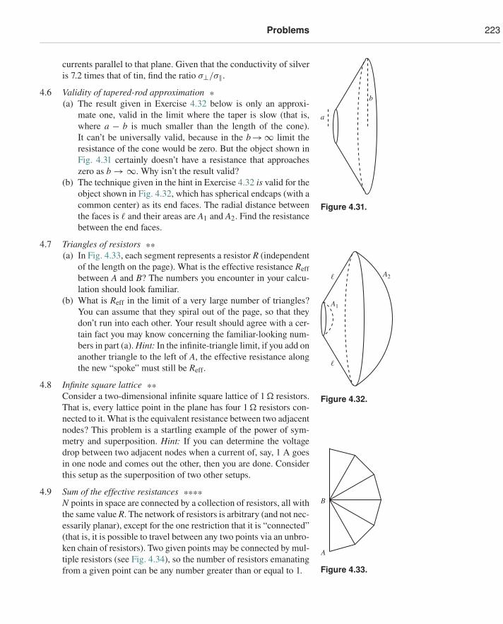
Problems 223
currents parallel to that plane. Given that the conductivity of silveris 7.2 times that of tin, find the ratio σ⊥/σ‖.
b
a
Figure 4.31.
4.6 Validity of tapered-rod approximation *(a) The result given in Exercise 4.32 below is only an approxi-
mate one, valid in the limit where the taper is slow (that is,where a − b is much smaller than the length of the cone).It can’t be universally valid, because in the b→∞ limit theresistance of the cone would be zero. But the object shown inFig. 4.31 certainly doesn’t have a resistance that approacheszero as b → ∞. Why isn’t the result valid?
(b) The technique given in the hint in Exercise 4.32 is valid for theobject shown in Fig. 4.32, which has spherical endcaps (with acommon center) as its end faces. The radial distance betweenthe faces is � and their areas are A1 and A2. Find the resistancebetween the end faces.
4.7 Triangles of resistors **(a) In Fig. 4.33, each segment represents a resistor R (independent
A1
A2
Figure 4.32.
of the length on the page). What is the effective resistance Reffbetween A and B? The numbers you encounter in your calcu-lation should look familiar.
(b) What is Reff in the limit of a very large number of triangles?You can assume that they spiral out of the page, so that theydon’t run into each other. Your result should agree with a cer-tain fact you may know concerning the familiar-looking num-bers in part (a). Hint: In the infinite-triangle limit, if you add onanother triangle to the left of A, the effective resistance alongthe new “spoke” must still be Reff.
4.8 Infinite square lattice **Consider a two-dimensional infinite square lattice of 1 � resistors.That is, every lattice point in the plane has four 1 � resistors con-nected to it. What is the equivalent resistance between two adjacentnodes? This problem is a startling example of the power of sym-metry and superposition. Hint: If you can determine the voltagedrop between two adjacent nodes when a current of, say, 1 A goesin one node and comes out the other, then you are done. Considerthis setup as the superposition of two other setups.
A
B
Figure 4.33.
4.9 Sum of the effective resistances ****N points in space are connected by a collection of resistors, all withthe same value R. The network of resistors is arbitrary (and not nec-essarily planar), except for the one restriction that it is “connected”(that is, it is possible to travel between any two points via an unbro-ken chain of resistors). Two given points may be connected by mul-tiple resistors (see Fig. 4.34), so the number of resistors emanatingfrom a given point can be any number greater than or equal to 1.
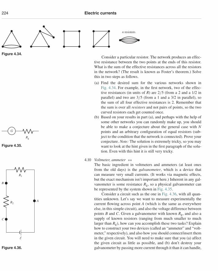
224 Electric currents
n resistors
Figure 4.34.Consider a particular resistor. The network produces an effec-
tive resistance between the two points at the ends of this resistor.What is the sum of the effective resistances across all the resistorsin the network? (The result is known as Foster’s theorem.) Solvethis in two steps as follows.
(a) Find the desired sum for the various networks shown inFig. 4.34. For example, in the first network, two of the effec-tive resistances (in units of R) are 2/5 (from a 2 and a 1/2 inparallel) and two are 3/5 (from a 1 and a 3/2 in parallel), sothe sum of all four effective resistances is 2. Remember thatthe sum is over all resistors and not pairs of points, so the twocurved resistors each get counted once.
(b) Based on your results in part (a), and perhaps with the help ofsome other networks you can randomly make up, you shouldbe able to make a conjecture about the general case with Npoints and an arbitrary configuration of equal resistors (sub-ject to the condition that the network is connected). Prove yourconjecture. Note: The solution is extremely tricky, so you maywant to look at the hint given in the first paragraph of the solu-tion. Even with this hint it is still very tricky.
Rg
G
Figure 4.35.
4.10 Voltmeter, ammeter **The basic ingredient in voltmeters and ammeters (at least onesfrom the old days) is the galvanometer, which is a device thatcan measure very small currents. (It works via magnetic effects,but the exact mechanism isn’t important here.) Inherent in any gal-vanometer is some resistance Rg, so a physical galvanometer canbe represented by the system shown in Fig. 4.35.
B
C
AR2
R1
E
Figure 4.36.
Consider a circuit such as the one in Fig. 4.36, with all quan-tities unknown. Let’s say we want to measure experimentally thecurrent flowing across point A (which is the same as everywhereelse, in this simple circuit), and also the voltage difference betweenpoints B and C. Given a galvanometer with known Rg, and also asupply of known resistors (ranging from much smaller to muchlarger than Rg), how can you accomplish these two tasks? Explainhow to construct your two devices (called an “ammeter” and “volt-meter,” respectively), and also how you should connect/insert themin the given circuit. You will need to make sure that you (a) affectthe given circuit as little as possible, and (b) don’t destroy yourgalvanometer by passing more current through it than it can handle,
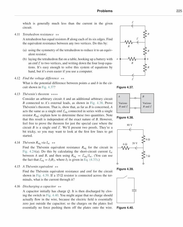
Problems 225
which is generally much less than the current in the givencircuit.
a b
R
R
R
R
R
E
E
E
Figure 4.37.
4.11 Tetrahedron resistance **A tetrahedron has equal resistors R along each of its six edges. Findthe equivalent resistance between any two vertices. Do this by:
(a) using the symmetry of the tetrahedron to reduce it to an equiv-alent resistor;
(b) laying the tetrahedron flat on a table, hooking up a battery withan emf E to two vertices, and writing down the four loop equa-tions. It’s easy enough to solve this system of equations byhand, but it’s even easier if you use a computer.
4.12 Find the voltage difference **What is the potential difference between points a and b in the cir-cuit shown in Fig. 4.37?
4.13 Thévenin’s theorem ****Consider an arbitrary circuit A and an additional arbitrary circuit
A B
Various R and E
Various R and E
Figure 4.38.
B connected to A’s external leads, as shown in Fig. 4.38. ProveThévenin’s theorem. That is, show that, as far as B is concerned, Aacts the same as a single emf Eeq connected in series with a singleresistor Req; explain how to determine these two quantities. Notethat this result is independent of the exact nature of B. However,feel free to prove the theorem for just the special case where thecircuit B is a single emf E . We’ll present two proofs. They’re abit tricky, so you may want to look at the first few lines to getstarted.
80 V
20 V6 Ω
7 Ω
6 Ω
Figure 4.39.
4.14 Thévenin Req via Isc **Find the Thévenin equivalent resistance Req for the circuit inFig. 4.24(a). Do this by calculating the short-circuit current Iscbetween A and B, and then using Req = Eeq/Isc. (You can usethe fact that Eeq = I3R3, where I3 is given in Eq. (4.33).)
4.15 A Thévenin equivalent **Find the Thévenin equivalent resistance and emf for the circuitshown in Fig. 4.39. If a 15 � resistor is connected across the ter-minals, what is the current through it?
Figure 4.40.
4.16 Discharging a capacitor **A capacitor initially has charge Q. It is then discharged by clos-ing the switch in Fig. 4.40. You might argue that no charge shouldactually flow in the wire, because the electric field is essentiallyzero just outside the capacitor; so the charges on the plates feelessentially no force pushing them off the plates onto the wire.
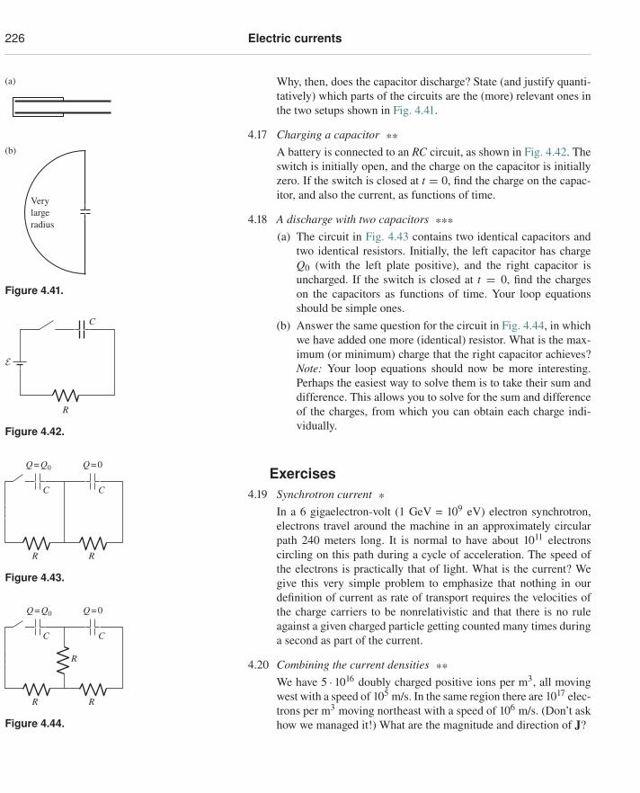
226 Electric currents
Why, then, does the capacitor discharge? State (and justify quanti-tatively) which parts of the circuits are the (more) relevant ones inthe two setups shown in Fig. 4.41.
(a)
(b)
Very large radius
Figure 4.41.
4.17 Charging a capacitor **A battery is connected to an RC circuit, as shown in Fig. 4.42. Theswitch is initially open, and the charge on the capacitor is initiallyzero. If the switch is closed at t = 0, find the charge on the capac-itor, and also the current, as functions of time.
4.18 A discharge with two capacitors ***(a) The circuit in Fig. 4.43 contains two identical capacitors and
two identical resistors. Initially, the left capacitor has chargeQ0 (with the left plate positive), and the right capacitor isuncharged. If the switch is closed at t = 0, find the chargeson the capacitors as functions of time. Your loop equationsshould be simple ones.
(b) Answer the same question for the circuit in Fig. 4.44, in whichwe have added one more (identical) resistor. What is the max-
R
C
E
Figure 4.42.
imum (or minimum) charge that the right capacitor achieves?Note: Your loop equations should now be more interesting.Perhaps the easiest way to solve them is to take their sum anddifference. This allows you to solve for the sum and differenceof the charges, from which you can obtain each charge indi-vidually.
Exercises4.19 Synchrotron current *
In a 6 gigaelectron-volt (1 GeV = 109 eV) electron synchrotron,
R
C C
R
Q = Q0 Q = 0
Figure 4.43.
electrons travel around the machine in an approximately circularpath 240 meters long. It is normal to have about 1011 electronscircling on this path during a cycle of acceleration. The speed ofthe electrons is practically that of light. What is the current? Wegive this very simple problem to emphasize that nothing in ourdefinition of current as rate of transport requires the velocities ofthe charge carriers to be nonrelativistic and that there is no ruleagainst a given charged particle getting counted many times during
R
R
C C
R
Q = Q0 Q = 0
Figure 4.44.
a second as part of the current.
4.20 Combining the current densities **We have 5 · 1016 doubly charged positive ions per m3, all movingwest with a speed of 105 m/s. In the same region there are 1017 elec-trons per m3 moving northeast with a speed of 106 m/s. (Don’t askhow we managed it!) What are the magnitude and direction of J?
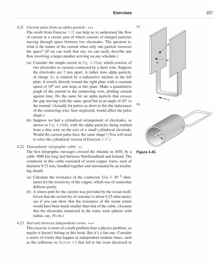
Exercises 227
4.21 Current pulse from an alpha particle ***The result from Exercise 3.37 can help us to understand the flowof current in a circuit, part of which consists of charged particlesmoving through space between two electrodes. The question is,what is the nature of the current when only one particle traversesthe space? (If we can work that out, we can easily describe anyflow involving a larger number arriving on any schedule.)
(a) Consider the simple circuit in Fig. 4.45(a), which consists of a
I
(a)
(b)
Figure 4.45.
two electrodes in vacuum connected by a short wire. Supposethe electrodes are 2 mm apart. A rather slow alpha particle,of charge 2e, is emitted by a radioactive nucleus in the leftplate. It travels directly toward the right plate with a constantspeed of 106 m/s and stops at this plate. Make a quantitativegraph of the current in the connecting wire, plotting currentagainst time. Do the same for an alpha particle that crossesthe gap moving with the same speed but at an angle of 45◦ tothe normal. (Actually for pulses as short as this the inductanceof the connecting wire, here neglected, would affect the pulseshape.)
(b) Suppose we had a cylindrical arrangement of electrodes, asshown in Fig. 4.45(b), with the alpha particles being emittedfrom a thin wire on the axis of a small cylindrical electrode.Would the current pulse have the same shape? (You will needto solve the cylindrical version of Exercise 3.37.)
4.22 Transatlantic telegraphic cable **The first telegraphic messages crossed the Atlantic in 1858, by acable 3000 km long laid between Newfoundland and Ireland. Theconductor in this cable consisted of seven copper wires, each ofdiameter 0.73 mm, bundled together and surrounded by an insulat-ing sheath.
(a) Calculate the resistance of the conductor. Use 3 · 10−8 ohm-meter for the resistivity of the copper, which was of somewhatdubious purity.
(b) A return path for the current was provided by the ocean itself.Given that the resistivity of seawater is about 0.25 ohm-meter,see if you can show that the resistance of the ocean returnwould have been much smaller than that of the cable. (Assumethat the electrodes immersed in the water were spheres withradius, say, 10 cm.)
4.23 Intervals between independent events ***This exercise is more of a math problem than a physics problem, somaybe it doesn’t belong in this book. But it’s a fun one. Considera series of events that happen at independent random times, suchas the collisions in Section 4.4 that led to the issue discussed in
228 Electric currents
Footnote 8. Such a process can be completely characterized by theprobability per unit time (call it p) of an event happening. Thedefinition of p is that the probability of an event happening in aninfinitesimal16 time dt equals p dt.
(a) Show that starting at any particular time (not necessarily thetime of an event), the probability that the next event happensbetween t and t + dt later equals e−ptp dt. You can do this bybreaking the time interval t into a large number of tiny inter-vals, and demanding that the event does not happen in any ofthem, but that it does happen in the following dt. (You willneed to use the fact that (1 − x/N)N = e−x in the N → ∞limit.) Verify that the integral of e−ptp dt correctly equals 1.
(b) Show that starting at any particular time (not necessarily thetime of an event), the average waiting time (also called theexpectation value of the waiting time) to the next event equals1/p. Explain why this is also the average time between events.
(c) Pick a random point in time, and look at the length of thetime interval (between successive events) that it belongs to.Explain, using the above results, why the average length ofthis interval is 2/p, and not 1/p.
(d) We have found that the average time between events is 1/p,and also that the average length of the interval surrounding arandomly chosen point in time is 2/p. Someone might thinkthat these two results should be the same. Explain intuitivelywhy they are not.
(e) Using the above probability distribution e−ptp dt properly, showmathematically why 2/p is the correct result for the averagelength of the interval surrounding a randomly chosen pointin time.
4.24 Mean free time in water *An ion in a liquid is so closely surrounded by neutral moleculesthat one can hardly speak of a “free time” between collisions. Still,it is interesting to see what value of τ is implied by Eq. (4.23) if wetake the observed conductivity of pure water from Table 4.1, andif we use 6 · 1019 m−3 for N+ and N−; see Footnote 4. A typicalthermal speed for a water molecule is 500 m/s. How far would ittravel in that time τ?
4.25 Drift velocity in seawater *The resistivity of seawater is about 0.25 ohm-meter. The chargecarriers are chiefly Na+ and Cl− ions, and of each there are about
16 The probability of an event happening in a noninfinitesimal time t is not equal to pt. If tis large enough, then pt is larger than 1, so it certainly can’t represent a probability. Inthat case, pt is the average number of events that occur in time t. But this doesn’t equalthe probability that an event occurs, because there can be double, triple, etc., events inthe time t. We don’t have to worry about multiple events if dt is infinitesimal.
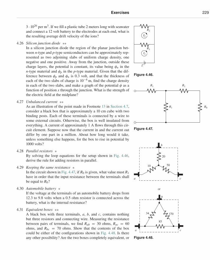
Exercises 229
3 · 1026 per m3. If we fill a plastic tube 2 meters long with seawaterand connect a 12 volt battery to the electrodes at each end, what isthe resulting average drift velocity of the ions?
4.26 Silicon junction diode **In a silicon junction diode the region of the planar junction bet-ween n-type and p-type semiconductors can be approximately rep-resented as two adjoining slabs of uniform charge density, onenegative and one positive. Away from the junction, outside thesecharge layers, the potential is constant, its value being φn in then-type material and φp in the p-type material. Given that the dif-ference between φp and φn is 0.3 volt, and that the thickness ofeach of the two slabs of charge is 10−4 m, find the charge densityin each of the two slabs, and make a graph of the potential φ as afunction of position x through the junction. What is the strength of
I1
I2
R2
R1
E
Figure 4.46.
the electric field at the midplane?
4.27 Unbalanced current **As an illustration of the point made in Footnote 13 in Section 4.7,consider a black box that is approximately a 10 cm cube with twobinding posts. Each of these terminals is connected by a wire tosome external circuits. Otherwise, the box is well insulated fromeverything. A current of approximately 1 A flows through this cir-cuit element. Suppose now that the current in and the current outdiffer by one part in a million. About how long would it take,unless something else happens, for the box to rise in potential by1000 volts?
4.28 Parallel resistors *By solving the loop equations for the setup shown in Fig. 4.46,derive the rule for adding resistors in parallel.
R1 R1
R1 R0
Figure 4.47.
4.29 Keeping the same resistance *In the circuit shown in Fig. 4.47, if R0 is given, what value must R1have in order that the input resistance between the terminals shallbe equal to R0?
4.30 Automobile battery *If the voltage at the terminals of an automobile battery drops from12.3 to 9.8 volts when a 0.5 ohm resistor is connected across thebattery, what is the internal resistance?
4.31 Equivalent boxes **A black box with three terminals, a, b, and c, contains nothingbut three resistors and connecting wire. Measuring the resistance
a c
b
20
50
or
10
34 170
85
ca
b
Figure 4.48.
between pairs of terminals, we find Rab = 30 ohms, Rac = 60ohms, and Rbc = 70 ohms. Show that the contents of the boxcould be either of the configurations shown in Fig. 4.48. Is thereany other possibility? Are the two boxes completely equivalent, or
230 Electric currents
is there an external measurement that would distinguish betweenthem?
4.32 Tapered rod *Two graphite rods are of equal length. One is a cylinder of radius a.The other is conical, tapering (or widening) linearly from radius aat one end to radius b at the other. Show that the end-to-end electri-cal resistance of the conical rod is a/b times that of the cylindricalrod. Hint: Consider the rod to be made up of thin, disk-like slices,all in series. (This result is actually only an approximate one, validin the limit where the taper is slow. See Problem 4.6 for a discus-sion of this.)
4.33 Laminated conductor extremum **(a) Consider the setup in Problem 4.5. For given conductivities
of the two materials, show that the ratio σ⊥/σ‖ is minimumwhen the layers have the same thickness (independent of whatthe conductivities are).
Give a physical argument why you would expect σ⊥/σ‖ toachieve a maximum or minimum somewhere between the twoextremes where one thickness is much larger/smaller than theother.
(b) For given layer thicknesses, show that the ratio σ⊥/σ‖ is max-imum when the materials have the same conductivity (inde-pendent of what the thicknesses are).
Give a physical argument why you would expect σ⊥/σ‖ toachieve a maximum or minimum somewhere between the twoextremes where one conductivity is much larger/smaller thanthe other.
4.34 Effective resistances in lattices **In the spirit of Problem 4.8, find the effective resistance betweentwo adjacent nodes in an infinite (a) 3D cubic lattice, (b) 2D tri-angular lattice, (c) 2D hexagonal lattice, (d) 1D lattice. (The lastof these tasks is a little silly, of course.) Assume that the latticesconsist of 1 � resistors.
4.35 Resistances in a cube **A cube has a resistor R along each edge. Find the equivalent resis-tance between two nodes that correspond to:
(a) diagonally opposite corners of the cube;(b) diagonally opposite corners of a face;(c) adjacent corners.
You do not need to solve a number of simultaneous equations;instead use symmetry arguments. Hint: If two vertices are at thesame potential, they can be collapsed to one point without chang-ing the equivalent resistance between the two given nodes.
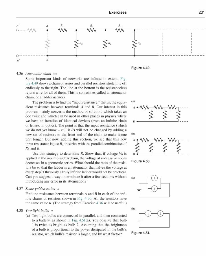
Exercises 231
A′ A
BB ′
R2 R2 R2
R1R1R1
Figure 4.49.
4.36 Attenuator chain **Some important kinds of networks are infinite in extent. Fig-ure 4.49 shows a chain of series and parallel resistors stretching offendlessly to the right. The line at the bottom is the resistancelessreturn wire for all of them. This is sometimes called an attenuatorchain, or a ladder network.
The problem is to find the “input resistance,” that is, the equiv-alent resistance between terminals A and B. Our interest in this A
(a)
(b)
B
A
B
Figure 4.50.
problem mainly concerns the method of solution, which takes anodd twist and which can be used in other places in physics wherewe have an iteration of identical devices (even an infinite chainof lenses, in optics). The point is that the input resistance (whichwe do not yet know – call it R) will not be changed by adding anew set of resistors to the front end of the chain to make it oneunit longer. But now, adding this section, we see that this newinput resistance is just R1 in series with the parallel combination ofR2 and R.
Use this strategy to determine R. Show that, if voltage V0 isapplied at the input to such a chain, the voltage at successive nodesdecreases in a geometric series. What should the ratio of the resis-tors be so that the ladder is an attenuator that halves the voltage atevery step? Obviously a truly infinite ladder would not be practical.Can you suggest a way to terminate it after a few sections withoutintroducing any error in its attenuation?
1 2
1
2
(a)
(b)
Figure 4.51.
4.37 Some golden ratios *Find the resistance between terminals A and B in each of the infi-nite chains of resistors shown in Fig. 4.50. All the resistors havethe same value R. (The strategy from Exercise 4.36 will be useful.)
4.38 Two light bulbs *(a) Two light bulbs are connected in parallel, and then connected
to a battery, as shown in Fig. 4.51(a). You observe that bulb1 is twice as bright as bulb 2. Assuming that the brightnessof a bulb is proportional to the power dissipated in the bulb’sresistor, which bulb’s resistor is larger, and by what factor?
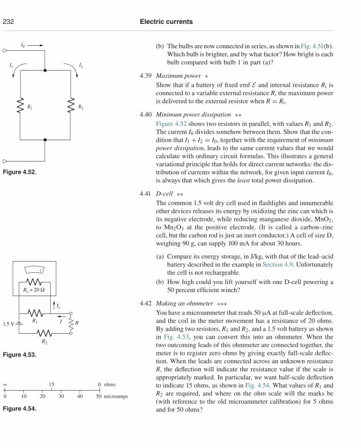
232 Electric currents
(b) The bulbs are now connected in series, as shown in Fig. 4.51(b).Which bulb is brighter, and by what factor? How bright is eachbulb compared with bulb 1 in part (a)?
4.39 Maximum power *Show that if a battery of fixed emf E and internal resistance Ri is
R1 R2
I2I1
I0
Figure 4.52.
connected to a variable external resistance R, the maximum poweris delivered to the external resistor when R = Ri.
4.40 Minimum power dissipation **Figure 4.52 shows two resistors in parallel, with values R1 and R2.The current I0 divides somehow between them. Show that the con-dition that I1 + I2 = I0, together with the requirement of minimumpower dissipation, leads to the same current values that we wouldcalculate with ordinary circuit formulas. This illustrates a generalvariational principle that holds for direct current networks: the dis-tribution of currents within the network, for given input current I0,is always that which gives the least total power dissipation.
4.41 D-cell **The common 1.5 volt dry cell used in flashlights and innumerableother devices releases its energy by oxidizing the zinc can which isits negative electrode, while reducing manganese dioxide, MnO2,to Mn2O3 at the positive electrode. (It is called a carbon–zinccell, but the carbon rod is just an inert conductor.) A cell of size D,weighing 90 g, can supply 100 mA for about 30 hours.
(a) Compare its energy storage, in J/kg, with that of the lead–acid
R1
R2
Rc = 20 Ω
R1.5 V I
Ic
Figure 4.53.
battery described in the example in Section 4.9. Unfortunatelythe cell is not rechargeable.
(b) How high could you lift yourself with one D-cell powering a50 percent efficient winch?
4.42 Making an ohmmeter ***You have a microammeter that reads 50 μA at full-scale deflection,and the coil in the meter movement has a resistance of 20 ohms.By adding two resistors, R1 and R2, and a 1.5 volt battery as shownin Fig. 4.53, you can convert this into an ohmmeter. When thetwo outcoming leads of this ohmmeter are connected together, themeter is to register zero ohms by giving exactly full-scale deflec-tion. When the leads are connected across an unknown resistanceR, the deflection will indicate the resistance value if the scale isappropriately marked. In particular, we want half-scale deflection
∞ 15
0 10 20 30 40 50
0 ohms
microamps
Figure 4.54.
to indicate 15 ohms, as shown in Fig. 4.54. What values of R1 andR2 are required, and where on the ohm scale will the marks be(with reference to the old microammeter calibration) for 5 ohmsand for 50 ohms?
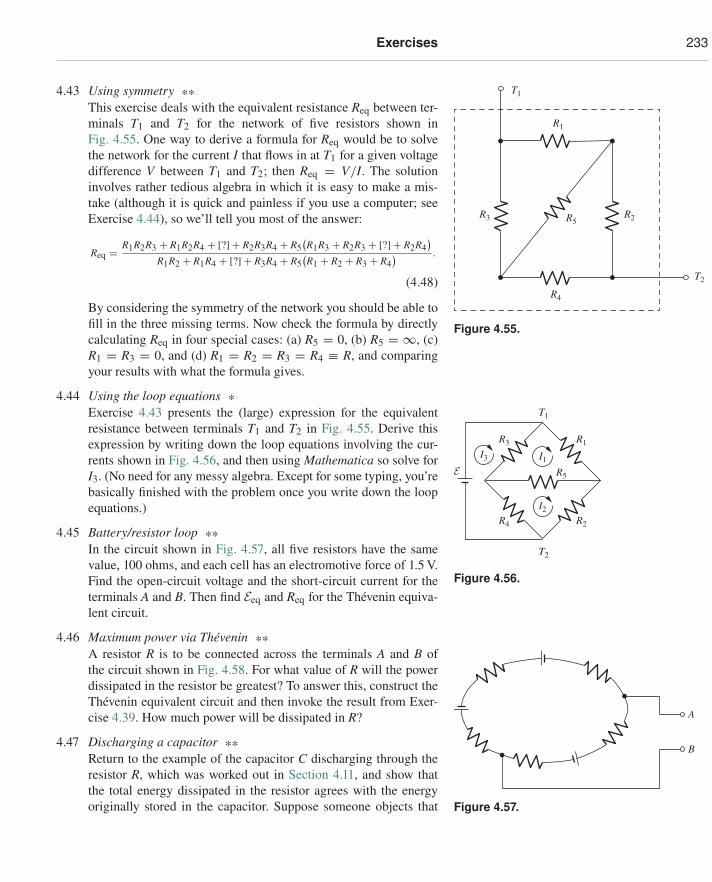
Exercises 233
4.43 Using symmetry **This exercise deals with the equivalent resistance Req between ter-minals T1 and T2 for the network of five resistors shown in
R3
T1
T2
R2R5
R1
R4
Figure 4.55.
Fig. 4.55. One way to derive a formula for Req would be to solvethe network for the current I that flows in at T1 for a given voltagedifference V between T1 and T2; then Req = V/I. The solutioninvolves rather tedious algebra in which it is easy to make a mis-take (although it is quick and painless if you use a computer; seeExercise 4.44), so we’ll tell you most of the answer:
Req = R1R2R3 + R1R2R4 + [?] + R2R3R4 + R5(R1R3 + R2R3 + [?] + R2R4
)R1R2 + R1R4 + [?] + R3R4 + R5
(R1 + R2 + R3 + R4
) .
(4.48)
By considering the symmetry of the network you should be able tofill in the three missing terms. Now check the formula by directlycalculating Req in four special cases: (a) R5 = 0, (b) R5 = ∞, (c)R1 = R3 = 0, and (d) R1 = R2 = R3 = R4 ≡ R, and comparingyour results with what the formula gives.
4.44 Using the loop equations *Exercise 4.43 presents the (large) expression for the equivalentresistance between terminals T1 and T2 in Fig. 4.55. Derive this
I3 I1
I2
R2
R1
T1
T2
R4
R5
R3
E
Figure 4.56.
expression by writing down the loop equations involving the cur-rents shown in Fig. 4.56, and then using Mathematica so solve forI3. (No need for any messy algebra. Except for some typing, you’rebasically finished with the problem once you write down the loopequations.)
4.45 Battery/resistor loop **In the circuit shown in Fig. 4.57, all five resistors have the samevalue, 100 ohms, and each cell has an electromotive force of 1.5 V.Find the open-circuit voltage and the short-circuit current for theterminals A and B. Then find Eeq and Req for the Thévenin equiva-lent circuit.
A
B
Figure 4.57.
4.46 Maximum power via Thévenin **A resistor R is to be connected across the terminals A and B ofthe circuit shown in Fig. 4.58. For what value of R will the powerdissipated in the resistor be greatest? To answer this, construct theThévenin equivalent circuit and then invoke the result from Exer-cise 4.39. How much power will be dissipated in R?
4.47 Discharging a capacitor **Return to the example of the capacitor C discharging through theresistor R, which was worked out in Section 4.11, and show thatthe total energy dissipated in the resistor agrees with the energyoriginally stored in the capacitor. Suppose someone objects that
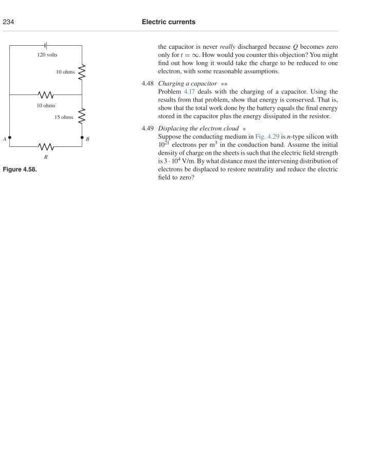
234 Electric currents
the capacitor is never really discharged because Q becomes zeroonly for t = ∞. How would you counter this objection? You might120 volts
10 ohms
15 ohms
10 ohms
A B
R
Figure 4.58.
find out how long it would take the charge to be reduced to oneelectron, with some reasonable assumptions.
4.48 Charging a capacitor **Problem 4.17 deals with the charging of a capacitor. Using theresults from that problem, show that energy is conserved. That is,show that the total work done by the battery equals the final energystored in the capacitor plus the energy dissipated in the resistor.
4.49 Displacing the electron cloud *Suppose the conducting medium in Fig. 4.29 is n-type silicon with1021 electrons per m3 in the conduction band. Assume the initialdensity of charge on the sheets is such that the electric field strengthis 3 · 104 V/m. By what distance must the intervening distribution ofelectrons be displaced to restore neutrality and reduce the electricfield to zero?
5The fields ofmoving charges
Overview The goal of this chapter is to show that when rela-tivity is combined with our theory of electricity, a necessary con-clusion is that a new force, the magnetic force, must exist. Innonstatic situations, charge is defined via a surface integral. Withthis definition, charge is invariant, that is, independent of refer-ence frame. Using this invariance, we determine how the electricfield transforms between two frames. We then calculate the elec-tric field due to a charge moving with constant velocity; it does notequal the spherically symmetric Coulomb field. Interesting fieldpatterns arise in cases where a charge starts or stops.
The main result of this chapter, derived in Section 5.9, is theexpression for the force that a moving charge (or a group of movingcharges) exerts on another moving charge. On our journey to thisresult, we will consider setups with increasing complexity. Moreprecisely, in calculating the force on a charge q due to anothercharge Q, there are four basic cases to consider, depending onthe charges’ motions. (1) If both charges are stationary in a givenframe, then we know from Chapter 1 that Coulomb’s law gives theforce. (2) If the source Q is moving and q is at rest, then we can usethe transformation rule for the electric field mentioned above. (3) Ifthe source Q is at rest and q is moving, then we can use the trans-formation rule for the force, presented in Appendix G, to show thatthe Coulomb field gives the force, as you would expect. (4) Finally,the case we are most concerned with: if both charges are moving,then we will show in Section 5.9 that a detailed consideration ofrelativistic effects implies that there exists an additional force thatmust be added to the electrical force; this is the magnetic force.
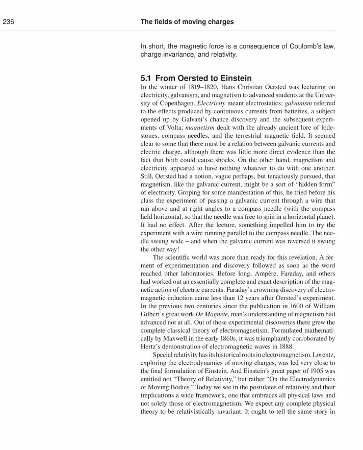
236 The fields of moving charges
In short, the magnetic force is a consequence of Coulomb’s law,charge invariance, and relativity.
5.1 From Oersted to EinsteinIn the winter of 1819–1820, Hans Christian Oersted was lecturing onelectricity, galvanism, and magnetism to advanced students at the Univer-sity of Copenhagen. Electricity meant electrostatics; galvanism referredto the effects produced by continuous currents from batteries, a subjectopened up by Galvani’s chance discovery and the subsequent experi-ments of Volta; magnetism dealt with the already ancient lore of lode-stones, compass needles, and the terrestrial magnetic field. It seemedclear to some that there must be a relation between galvanic currents andelectric charge, although there was little more direct evidence than thefact that both could cause shocks. On the other hand, magnetism andelectricity appeared to have nothing whatever to do with one another.Still, Oersted had a notion, vague perhaps, but tenaciously pursued, thatmagnetism, like the galvanic current, might be a sort of “hidden form”of electricity. Groping for some manifestation of this, he tried before hisclass the experiment of passing a galvanic current through a wire thatran above and at right angles to a compass needle (with the compassheld horizontal, so that the needle was free to spin in a horizontal plane).It had no effect. After the lecture, something impelled him to try theexperiment with a wire running parallel to the compass needle. The nee-dle swung wide – and when the galvanic current was reversed it swungthe other way!
The scientific world was more than ready for this revelation. A fer-ment of experimentation and discovery followed as soon as the wordreached other laboratories. Before long, Ampère, Faraday, and othershad worked out an essentially complete and exact description of the mag-netic action of electric currents. Faraday’s crowning discovery of electro-magnetic induction came less than 12 years after Oersted’s experiment.In the previous two centuries since the publication in 1600 of WilliamGilbert’s great work De Magnete, man’s understanding of magnetism hadadvanced not at all. Out of these experimental discoveries there grew thecomplete classical theory of electromagnetism. Formulated mathemati-cally by Maxwell in the early 1860s, it was triumphantly corroborated byHertz’s demonstration of electromagnetic waves in 1888.
Special relativityhas itshistorical roots inelectromagnetism.Lorentz,exploring the electrodynamics of moving charges, was led very close tothe final formulation of Einstein. And Einstein’s great paper of 1905 wasentitled not “Theory of Relativity,” but rather “On the Electrodynamicsof Moving Bodies.” Today we see in the postulates of relativity and theirimplications a wide framework, one that embraces all physical laws andnot solely those of electromagnetism. We expect any complete physicaltheory to be relativistically invariant. It ought to tell the same story in
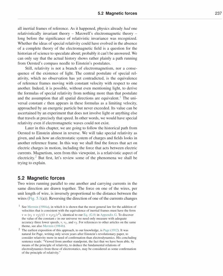
5.2 Magnetic forces 237
all inertial frames of reference. As it happened, physics already had onerelativistically invariant theory – Maxwell’s electromagnetic theory –long before the significance of relativistic invariance was recognized.Whether the ideas of special relativity could have evolved in the absenceof a complete theory of the electromagnetic field is a question for thehistorian of science to speculate about; probably it can’t be answered. Wecan only say that the actual history shows rather plainly a path runningfrom Oersted’s compass needle to Einstein’s postulates.
Still, relativity is not a branch of electromagnetism, nor a conse-quence of the existence of light. The central postulate of special rel-ativity, which no observation has yet contradicted, is the equivalenceof reference frames moving with constant velocity with respect to oneanother. Indeed, it is possible, without even mentioning light, to derivethe formulas of special relativity from nothing more than that postulateand the assumption that all spatial directions are equivalent.1 The uni-versal constant c then appears in these formulas as a limiting velocity,approached by an energetic particle but never exceeded. Its value can beascertained by an experiment that does not involve light or anything elsethat travels at precisely that speed. In other words, we would have specialrelativity even if electromagnetic waves could not exist.
Later in this chapter, we are going to follow the historical path fromOersted to Einstein almost in reverse. We will take special relativity asgiven, and ask how an electrostatic system of charges and fields looks inanother reference frame. In this way we shall find the forces that act onelectric charges in motion, including the force that acts between electriccurrents. Magnetism, seen from this viewpoint, is a relativistic aspect ofelectricity.2 But first, let’s review some of the phenomena we shall betrying to explain.
5.2 Magnetic forcesTwo wires running parallel to one another and carrying currents in thesame direction are drawn together. The force on one of the wires, perunit length of wire, is inversely proportional to the distance between thewires (Fig. 5.1(a)). Reversing the direction of one of the currents changes
1 See Mermin (1984a), in which it is shown that the most general law for the addition ofvelocities that is consistent with the equivalence of inertial frames must have the formv = (v1 + v2)/(1 + v1v2/c2), identical to our Eq. (G.8) in Appendix G. To discoverthe value of the constant c in our universe we need only measure with adequateaccuracy three lower speeds, v, v1, and v2. For references to other articles on the sametheme, see also Mermin (1984b).
2 The earliest exposition of this approach, to our knowledge, is Page (1912). It wasnatural for Page, writing only seven years after Einstein’s revolutionary paper, toconsider relativity more in need of confirmation than electrodynamics. His concludingsentence reads: “Viewed from another standpoint, the fact that we have been able, bymeans of the principle of relativity, to deduce the fundamental relations ofelectrodynamics from those of electrostatics, may be considered as some confirmationof the principle of relativity.”
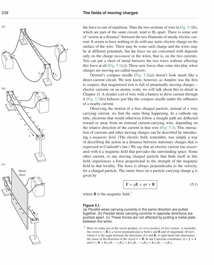
238 The fields of moving charges
the force to one of repulsion. Thus the two sections of wire in Fig. 5.1(b),which are part of the same circuit, tend to fly apart. There is some sortof “action at a distance” between the two filaments of steady electric cur-rent. It seems to have nothing to do with any static electric charge on thesurface of the wire. There may be some such charge and the wires maybe at different potentials, but the force we are concerned with dependsonly on the charge movement in the wires, that is, on the two currents.You can put a sheet of metal between the two wires without affectingthis force at all (Fig. 5.1(c)). These new forces that come into play whencharges are moving are called magnetic.
+– +
–
I1 I2
(a)
(b)
+
–
I
I
(c)
+
–
I
I
Metalsheet
Oersted’s compass needle (Fig. 5.2(a)) doesn’t look much like adirect-current circuit. We now know, however, as Ampère was the firstto suspect, that magnetized iron is full of perpetually moving charges –electric currents on an atomic scale; we will talk about this in detail inChapter 11. A slender coil of wire with a battery to drive current throughit (Fig. 5.2(b)) behaves just like the compass needle under the influenceof a nearby current.
Observing the motion of a free charged particle, instead of a wirecarrying current, we find the same thing happening. In a cathode raytube, electrons that would otherwise follow a straight path are deflectedtoward or away from an external current-carrying wire, depending onthe relative direction of the current in that wire (Fig. 5.3). This interac-tion of currents and other moving charges can be described by introduc-ing a magnetic field. (The electric field, remember, was simply a wayof describing the action at a distance between stationary charges that isexpressed in Coulomb’s law.) We say that an electric current has associ-ated with it a magnetic field that pervades the surrounding space. Someother current, or any moving charged particle that finds itself in thisfield, experiences a force proportional to the strength of the magneticfield in that locality. The force is always perpendicular to the velocity,for a charged particle. The entire force on a particle carrying charge q isgiven by
F = qE + qv × B (5.1)
where B is the magnetic field.3
Figure 5.1.(a) Parallel wires carrying currents in the same direction are pulledtogether. (b) Parallel wires carrying currents in opposite directions arepushed apart. (c) These forces are not affected by putting a metal platebetween the wires.3 Here we make use of the vector product, or cross product, of two vectors. A reminder:
the vector v × B is a vector perpendicular to both v and B and of magnitude vB sin θ ,where θ is the angle between the directions of v and B. A right-hand rule determinesthe sense of the direction of the vector v × B. In our Cartesian coordinates, x × y = zand v × B = x(vyBz − vzBy) + y(vzBx − vxBz) + z(vxBy − vyBx).
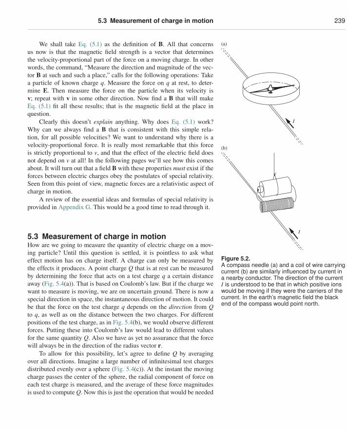
5.3 Measurement of charge in motion 239
We shall take Eq. (5.1) as the definition of B. All that concernsus now is that the magnetic field strength is a vector that determinesthe velocity-proportional part of the force on a moving charge. In otherwords, the command, “Measure the direction and magnitude of the vec-tor B at such and such a place,” calls for the following operations: Takea particle of known charge q. Measure the force on q at rest, to deter-mine E. Then measure the force on the particle when its velocity isv; repeat with v in some other direction. Now find a B that will makeEq. (5.1) fit all these results; that is the magnetic field at the place inquestion.
I
(a)
(b)
I
Figure 5.2.A compass needle (a) and a coil of wire carryingcurrent (b) are similarly influenced by current ina nearby conductor. The direction of the currentI is understood to be that in which positive ionswould be moving if they were the carriers of thecurrent. In the earth’s magnetic field the blackend of the compass would point north.
Clearly this doesn’t explain anything. Why does Eq. (5.1) work?Why can we always find a B that is consistent with this simple rela-tion, for all possible velocities? We want to understand why there is avelocity-proportional force. It is really most remarkable that this forceis strictly proportional to v, and that the effect of the electric field doesnot depend on v at all! In the following pages we’ll see how this comesabout. It will turn out that a field B with these properties must exist if theforces between electric charges obey the postulates of special relativity.Seen from this point of view, magnetic forces are a relativistic aspect ofcharge in motion.
A review of the essential ideas and formulas of special relativity isprovided in Appendix G. This would be a good time to read through it.
5.3 Measurement of charge in motionHow are we going to measure the quantity of electric charge on a mov-ing particle? Until this question is settled, it is pointless to ask whateffect motion has on charge itself. A charge can only be measured bythe effects it produces. A point charge Q that is at rest can be measuredby determining the force that acts on a test charge q a certain distanceaway (Fig. 5.4(a)). That is based on Coulomb’s law. But if the charge wewant to measure is moving, we are on uncertain ground. There is now aspecial direction in space, the instantaneous direction of motion. It couldbe that the force on the test charge q depends on the direction from Qto q, as well as on the distance between the two charges. For differentpositions of the test charge, as in Fig. 5.4(b), we would observe differentforces. Putting these into Coulomb’s law would lead to different valuesfor the same quantity Q. Also we have as yet no assurance that the forcewill always be in the direction of the radius vector r.
To allow for this possibility, let’s agree to define Q by averagingover all directions. Imagine a large number of infinitesimal test chargesdistributed evenly over a sphere (Fig. 5.4(c)). At the instant the movingcharge passes the center of the sphere, the radial component of force oneach test charge is measured, and the average of these force magnitudesis used to compute Q. Now this is just the operation that would be needed
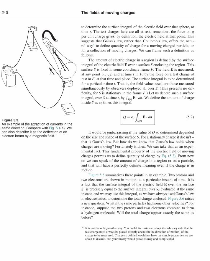
240 The fields of moving charges
to determine the surface integral of the electric field over that sphere, attime t. The test charges here are all at rest, remember; the force on qper unit charge gives, by definition, the electric field at that point. Thissuggests that Gauss’s law, rather than Coulomb’s law, offers the natu-ral way4 to define quantity of charge for a moving charged particle, orfor a collection of moving charges. We can frame such a definition asfollows.
The amount of electric charge in a region is defined by the surfaceintegral of the electric field E over a surface S enclosing the region. Thissurface S is fixed in some coordinate frame F. The field E is measured,at any point (x, y, z) and at time t in F, by the force on a test charge atrest in F, at that time and place. The surface integral is to be determinedfor a particular time t. That is, the field values used are those measuredsimultaneously by observers deployed all over S. (This presents no dif-ficulty, for S is stationary in the frame F.) Let us denote such a surfaceintegral, over S at time t, by
∫S(t) E · da. We define the amount of charge
inside S as ε0 times this integral:
Q = ε0
∫S(t)
E · da (5.2)
+–
I
Figure 5.3.An example of the attraction of currents in thesame direction. Compare with Fig. 5.1(a). Wecan also describe it as the deflection of anelectron beam by a magnetic field.
It would be embarrassing if the value of Q so determined dependedon the size and shape of the surface S. For a stationary charge it doesn’t –that is Gauss’s law. But how do we know that Gauss’s law holds whencharges are moving? Fortunately it does. We can take that as an exper-imental fact. This fundamental property of the electric field of movingcharges permits us to define quantity of charge by Eq. (5.2). From nowon we can speak of the amount of charge in a region or on a particle,and that will have a perfectly definite meaning even if the charge is inmotion.
Figure 5.5 summarizes these points in an example. Two protons andtwo electrons are shown in motion, at a particular instant of time. It isa fact that the surface integral of the electric field E over the surfaceS1 is precisely equal to the surface integral over S2 evaluated at the sameinstant, and we may use this integral, as we have always used Gauss’s lawin electrostatics, to determine the total charge enclosed. Figure 5.6 raisesa new question. What if the same particles had some other velocities? Forinstance, suppose the two protons and two electrons combine to forma hydrogen molecule. Will the total charge appear exactly the same asbefore?
4 It is not the only possible way. You could, for instance, adopt the arbitrary rule that thetest charge must always be placed directly ahead (in the direction of motion) of thecharge to be measured. Charge so defined would not have the simple properties we areabout to discuss. and your theory would prove clumsy and complicated.
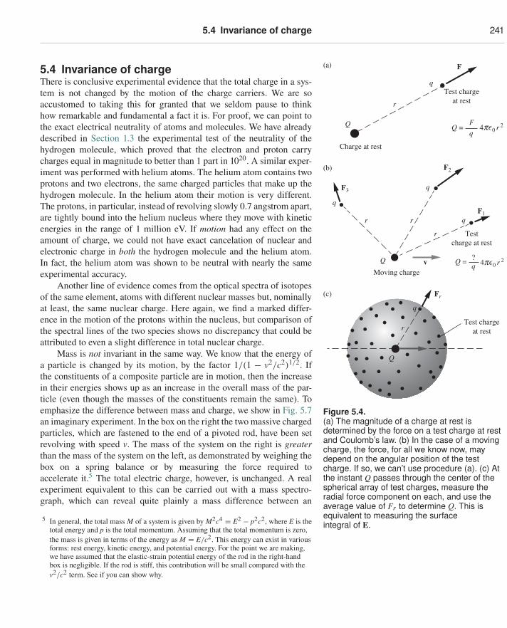
5.4 Invariance of charge 241
q
F
r
Q
Charge at rest
Q = r 2F
Test chargeat rest
q
(a)
q
q
q
F3
F2
F1r r
r
vQ
Testcharge at rest
Moving chargeQ = ?
q
(b)
r 2
q
Fr
r
Q
Test chargeat rest
(c)
Figure 5.4.(a) The magnitude of a charge at rest isdetermined by the force on a test charge at restand Coulomb’s law. (b) In the case of a movingcharge, the force, for all we know now, maydepend on the angular position of the testcharge. If so, we can’t use procedure (a). (c) Atthe instant Q passes through the center of thespherical array of test charges, measure theradial force component on each, and use theaverage value of Fr to determine Q. This isequivalent to measuring the surfaceintegral of E.
5.4 Invariance of chargeThere is conclusive experimental evidence that the total charge in a sys-tem is not changed by the motion of the charge carriers. We are soaccustomed to taking this for granted that we seldom pause to thinkhow remarkable and fundamental a fact it is. For proof, we can point tothe exact electrical neutrality of atoms and molecules. We have alreadydescribed in Section 1.3 the experimental test of the neutrality of thehydrogen molecule, which proved that the electron and proton carrycharges equal in magnitude to better than 1 part in 1020. A similar exper-iment was performed with helium atoms. The helium atom contains twoprotons and two electrons, the same charged particles that make up thehydrogen molecule. In the helium atom their motion is very different.The protons, in particular, instead of revolving slowly 0.7 angstrom apart,are tightly bound into the helium nucleus where they move with kineticenergies in the range of 1 million eV. If motion had any effect on theamount of charge, we could not have exact cancelation of nuclear andelectronic charge in both the hydrogen molecule and the helium atom.In fact, the helium atom was shown to be neutral with nearly the sameexperimental accuracy.
Another line of evidence comes from the optical spectra of isotopesof the same element, atoms with different nuclear masses but, nominallyat least, the same nuclear charge. Here again, we find a marked differ-ence in the motion of the protons within the nucleus, but comparison ofthe spectral lines of the two species shows no discrepancy that could beattributed to even a slight difference in total nuclear charge.
Mass is not invariant in the same way. We know that the energy ofa particle is changed by its motion, by the factor 1/(1 − v2/c2)1/2. Ifthe constituents of a composite particle are in motion, then the increasein their energies shows up as an increase in the overall mass of the par-ticle (even though the masses of the constituents remain the same). Toemphasize the difference between mass and charge, we show in Fig. 5.7an imaginary experiment. In the box on the right the two massive chargedparticles, which are fastened to the end of a pivoted rod, have been setrevolving with speed v. The mass of the system on the right is greaterthan the mass of the system on the left, as demonstrated by weighing thebox on a spring balance or by measuring the force required toaccelerate it.5 The total electric charge, however, is unchanged. A realexperiment equivalent to this can be carried out with a mass spectro-graph, which can reveal quite plainly a mass difference between an
5 In general, the total mass M of a system is given by M2c4 = E2 − p2c2, where E is thetotal energy and p is the total momentum. Assuming that the total momentum is zero,the mass is given in terms of the energy as M = E/c2. This energy can exist in variousforms: rest energy, kinetic energy, and potential energy. For the point we are making,we have assumed that the elastic-strain potential energy of the rod in the right-handbox is negligible. If the rod is stiff, this contribution will be small compared with thev2/c2 term. See if you can show why.
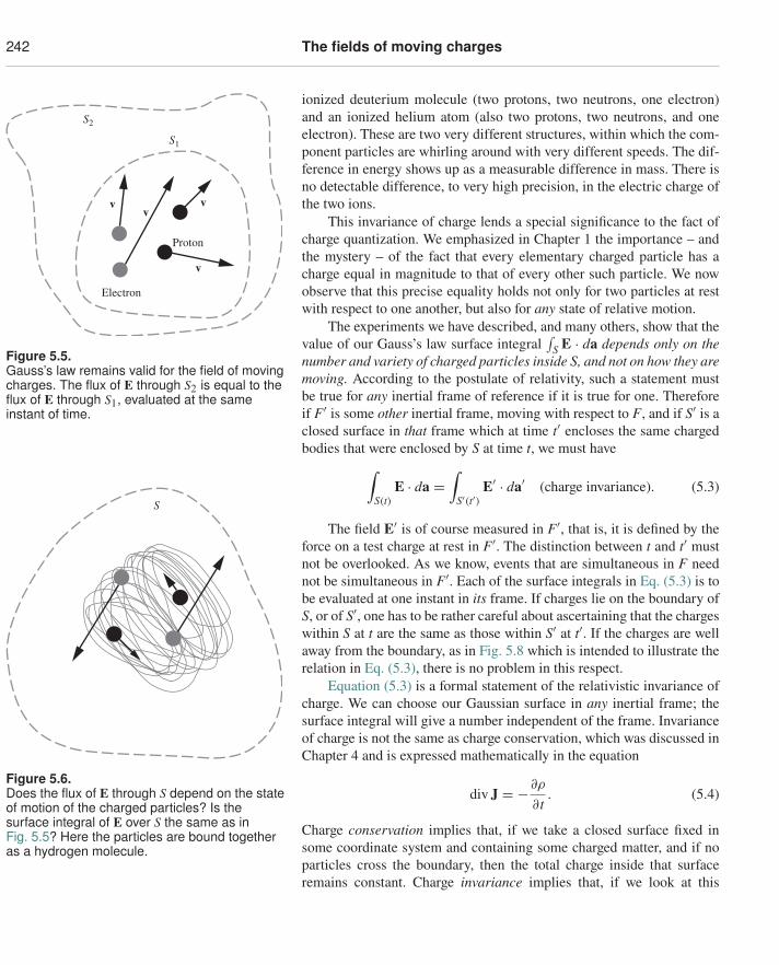
242 The fields of moving charges
ionized deuterium molecule (two protons, two neutrons, one electron)and an ionized helium atom (also two protons, two neutrons, and oneelectron). These are two very different structures, within which the com-ponent particles are whirling around with very different speeds. The dif-ference in energy shows up as a measurable difference in mass. There isno detectable difference, to very high precision, in the electric charge ofthe two ions.
Proton
Electron
S1
vv
v
v
S2
Figure 5.5.Gauss’s law remains valid for the field of movingcharges. The flux of E through S2 is equal to theflux of E through S1, evaluated at the sameinstant of time.
This invariance of charge lends a special significance to the fact ofcharge quantization. We emphasized in Chapter 1 the importance – andthe mystery – of the fact that every elementary charged particle has acharge equal in magnitude to that of every other such particle. We nowobserve that this precise equality holds not only for two particles at restwith respect to one another, but also for any state of relative motion.
The experiments we have described, and many others, show that thevalue of our Gauss’s law surface integral
∫S E · da depends only on the
number and variety of charged particles inside S, and not on how they aremoving. According to the postulate of relativity, such a statement mustbe true for any inertial frame of reference if it is true for one. Thereforeif F′ is some other inertial frame, moving with respect to F, and if S′ is aclosed surface in that frame which at time t′ encloses the same chargedbodies that were enclosed by S at time t, we must have∫
S(t)E · da =
∫S′(t′)
E′ · da′ (charge invariance). (5.3)S
Figure 5.6.Does the flux of E through S depend on the stateof motion of the charged particles? Is thesurface integral of E over S the same as inFig. 5.5? Here the particles are bound togetheras a hydrogen molecule.
The field E′ is of course measured in F′, that is, it is defined by theforce on a test charge at rest in F′. The distinction between t and t′ mustnot be overlooked. As we know, events that are simultaneous in F neednot be simultaneous in F′. Each of the surface integrals in Eq. (5.3) is tobe evaluated at one instant in its frame. If charges lie on the boundary ofS, or of S′, one has to be rather careful about ascertaining that the chargeswithin S at t are the same as those within S′ at t′. If the charges are wellaway from the boundary, as in Fig. 5.8 which is intended to illustrate therelation in Eq. (5.3), there is no problem in this respect.
Equation (5.3) is a formal statement of the relativistic invariance ofcharge. We can choose our Gaussian surface in any inertial frame; thesurface integral will give a number independent of the frame. Invarianceof charge is not the same as charge conservation, which was discussed inChapter 4 and is expressed mathematically in the equation
div J = −∂ρ
∂t. (5.4)
Charge conservation implies that, if we take a closed surface fixed insome coordinate system and containing some charged matter, and if noparticles cross the boundary, then the total charge inside that surfaceremains constant. Charge invariance implies that, if we look at this
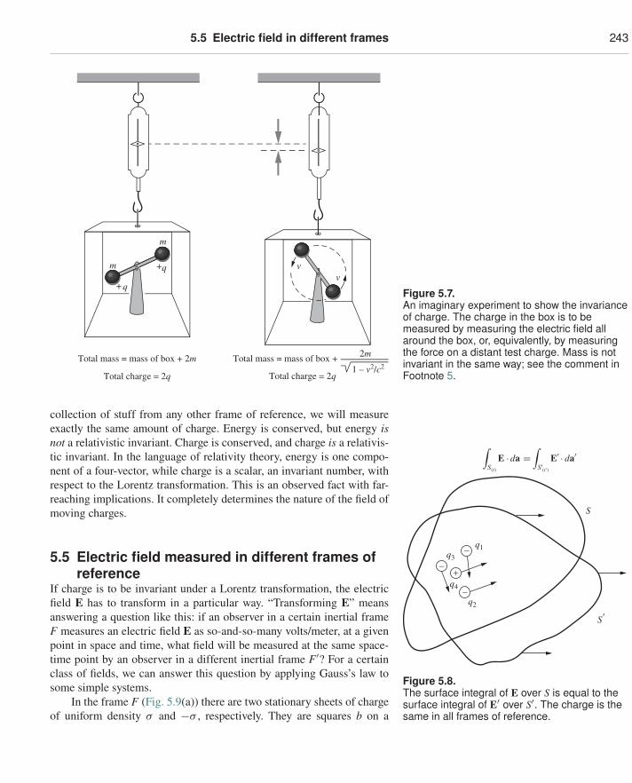
5.5 Electric field in different frames 243
m
m
q
q+
+v
v
Total mass = mass of box + 2m
Total charge = 2q
Total mass = mass of box +
Total charge = 2q1 – v2/c2
2m
Figure 5.7.An imaginary experiment to show the invarianceof charge. The charge in the box is to bemeasured by measuring the electric field allaround the box, or, equivalently, by measuringthe force on a distant test charge. Mass is notinvariant in the same way; see the comment inFootnote 5.
collection of stuff from any other frame of reference, we will measureexactly the same amount of charge. Energy is conserved, but energy isnot a relativistic invariant. Charge is conserved, and charge is a relativis-tic invariant. In the language of relativity theory, energy is one compo-nent of a four-vector, while charge is a scalar, an invariant number, withrespect to the Lorentz transformation. This is an observed fact with far-reaching implications. It completely determines the nature of the field ofmoving charges.
+
–
–
– q1
q2
S�
S
q3
q4
Figure 5.8.The surface integral of E over S is equal to thesurface integral of E′ over S′. The charge is thesame in all frames of reference.
5.5 Electric field measured in different frames ofreference
If charge is to be invariant under a Lorentz transformation, the electricfield E has to transform in a particular way. “Transforming E” meansanswering a question like this: if an observer in a certain inertial frameF measures an electric field E as so-and-so-many volts/meter, at a givenpoint in space and time, what field will be measured at the same space-time point by an observer in a different inertial frame F′? For a certainclass of fields, we can answer this question by applying Gauss’s law tosome simple systems.
In the frame F (Fig. 5.9(a)) there are two stationary sheets of chargeof uniform density σ and −σ , respectively. They are squares b on a
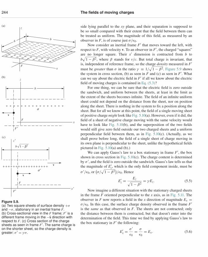
244 The fields of moving charges
side lying parallel to the xy plane, and their separation is supposed tobe so small compared with their extent that the field between them canbe treated as uniform. The magnitude of this field, as measured by anobserver in F, is of course just σ/ε0.
Fx
z(a)
bb
F
s
v
x
z
F ′
+ + + + + + + + + + + + + + + +
(b)
b
s ′
1 − b2b
F ′
− − − − − − − − − − − − − − − − −
+ + + + + + + + + + + + + + + + + +
F
x ′
v
v
z ′(c)
Figure 5.9.(a) Two square sheets of surface density +σand −σ , stationary in an inertial frame F.(b) Cross-sectional view in the F frame; F′ is adifferent frame moving in the −x direction withrespect to F. (c) Cross section of the chargesheets as seen in frame F′. The same charge ison the shorter sheet, so the charge density isgreater: σ ′ = γ σ .
Now consider an inertial frame F′ that moves toward the left, withrespect to F, with velocity v. To an observer in F′, the charged “squares”are no longer square. Their x′ dimension is contracted from b tob√
1 − β2, where β stands for v/c. But total charge is invariant, thatis, independent of reference frame, so the charge density measured in F′must be greater than σ in the ratio γ ≡ 1/
√1 − β2. Figure 5.9 shows
the system in cross section, (b) as seen in F and (c) as seen in F′. Whatcan we say about the electric field in F′ if all we know about the electricfield of moving charges is contained in Eq. (5.3)?
For one thing, we can be sure that the electric field is zero outsidethe sandwich, and uniform between the sheets, at least in the limit asthe extent of the sheets becomes infinite. The field of an infinite uniformsheet could not depend on the distance from the sheet, nor on positionalong the sheet. There is nothing in the system to fix a position along thesheet. But for all we know at this point, the field of a single moving sheetof positive charge might look like Fig. 5.10(a). However, even if it did, thefield of a sheet of negative charge moving with the same velocity wouldhave to look like Fig. 5.10(b), and the superposition of the two fieldswould still give zero field outside our two charged sheets and a uniformperpendicular field between them, as in Fig. 5.10(c). (Actually, as weshall prove before long, the field of a single sheet of charge moving inits own plane is perpendicular to the sheet, unlike the hypothetical fieldspictured in Fig. 5.10(a) and (b).)
We can apply Gauss’s law to a box stationary in frame F′, the boxshown in cross section in Fig. 5.10(c). The charge content is determinedby σ ′, and the field is zero outside the sandwich. Gauss’s law tells us thatthe magnitude of E′
z, which is the only field component inside, must beσ ′/ε0, or
(σ/
√1 − β2
)/ε0. Hence
E′z =
Ez√1 − β2
= γ Ez. (5.5)
Now imagine a different situation with the stationary charged sheetsin the frame F oriented perpendicular to the x axis, as in Fig. 5.11. Theobserver in F now reports a field in the x direction of magnitude Ex =σ/ε0. In this case, the surface charge density observed in the frame F′is the same as that observed in F. The sheets are not contracted; onlythe distance between them is contracted, but that doesn’t enter into thedetermination of the field. This time we find by applying Gauss’s law tothe box stationary in F′ the following:
E′x =
σ ′
ε0= σ
ε0= Ex. (5.6)
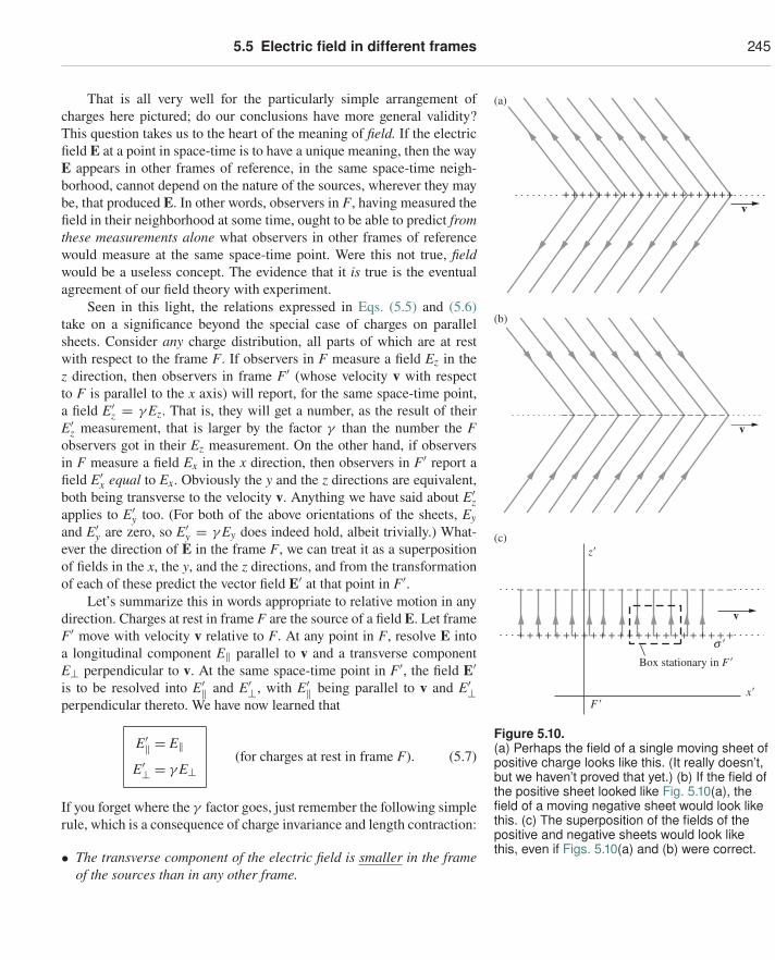
5.5 Electric field in different frames 245
That is all very well for the particularly simple arrangement ofcharges here pictured; do our conclusions have more general validity?This question takes us to the heart of the meaning of field. If the electricfield E at a point in space-time is to have a unique meaning, then the wayE appears in other frames of reference, in the same space-time neigh-borhood, cannot depend on the nature of the sources, wherever they maybe, that produced E. In other words, observers in F, having measured thefield in their neighborhood at some time, ought to be able to predict fromthese measurements alone what observers in other frames of referencewould measure at the same space-time point. Were this not true, fieldwould be a useless concept. The evidence that it is true is the eventualagreement of our field theory with experiment.
+ + + + + + + + + + + + + + + + + ++++v
(a)
– – – – – – – – – – – – – – – – – – – – –
(b)
v
+
– – – – – – – – – – – – – – – – – – – – – – – –
+ + + + + + + + + + + + + + + + + + + + + + +s �
Box stationary in F�
(c)
v
F�
z�
x�
Figure 5.10.(a) Perhaps the field of a single moving sheet ofpositive charge looks like this. (It really doesn’t,but we haven’t proved that yet.) (b) If the field ofthe positive sheet looked like Fig. 5.10(a), thefield of a moving negative sheet would look likethis. (c) The superposition of the fields of thepositive and negative sheets would look likethis, even if Figs. 5.10(a) and (b) were correct.
Seen in this light, the relations expressed in Eqs. (5.5) and (5.6)take on a significance beyond the special case of charges on parallelsheets. Consider any charge distribution, all parts of which are at restwith respect to the frame F. If observers in F measure a field Ez in thez direction, then observers in frame F′ (whose velocity v with respectto F is parallel to the x axis) will report, for the same space-time point,a field E′
z = γ Ez. That is, they will get a number, as the result of theirE′
z measurement, that is larger by the factor γ than the number the Fobservers got in their Ez measurement. On the other hand, if observersin F measure a field Ex in the x direction, then observers in F′ report afield E′
x equal to Ex. Obviously the y and the z directions are equivalent,both being transverse to the velocity v. Anything we have said about E′
zapplies to E′
y too. (For both of the above orientations of the sheets, Eyand E′
y are zero, so E′y = γ Ey does indeed hold, albeit trivially.) What-
ever the direction of E in the frame F, we can treat it as a superpositionof fields in the x, the y, and the z directions, and from the transformationof each of these predict the vector field E′ at that point in F′.
Let’s summarize this in words appropriate to relative motion in anydirection. Charges at rest in frame F are the source of a field E. Let frameF′ move with velocity v relative to F. At any point in F, resolve E intoa longitudinal component E‖ parallel to v and a transverse componentE⊥ perpendicular to v. At the same space-time point in F′, the field E′is to be resolved into E′‖ and E′⊥, with E′‖ being parallel to v and E′⊥perpendicular thereto. We have now learned that
E′‖ = E‖E′⊥ = γ E⊥
(for charges at rest in frame F). (5.7)
If you forget where the γ factor goes, just remember the following simplerule, which is a consequence of charge invariance and length contraction:
• The transverse component of the electric field is smaller in the frameof the sources than in any other frame.
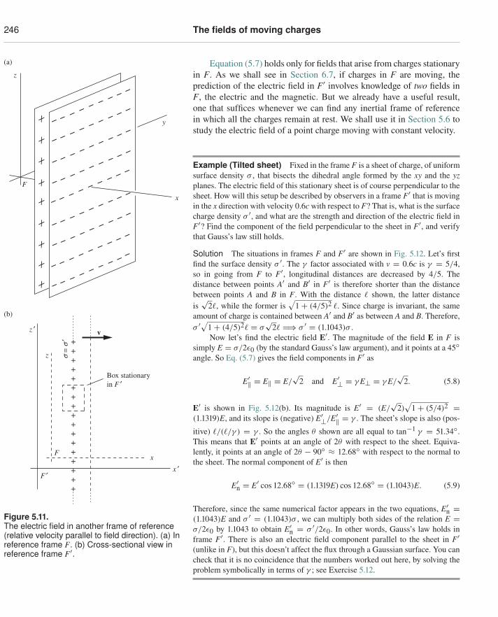
246 The fields of moving charges
Equation (5.7) holds only for fields that arise from charges stationaryin F. As we shall see in Section 6.7, if charges in F are moving, theprediction of the electric field in F′ involves knowledge of two fields inF, the electric and the magnetic. But we already have a useful result,one that suffices whenever we can find any inertial frame of referencein which all the charges remain at rest. We shall use it in Section 5.6 tostudy the electric field of a point charge moving with constant velocity.
+
+
+
++
+
+++
F
y
x
(a)
z
+++++++++++++++++
v
Box stationaryin F ′
s =
s′
F
F¢
z
z ′
x ′x
(b)
Figure 5.11.The electric field in another frame of reference(relative velocity parallel to field direction). (a) Inreference frame F. (b) Cross-sectional view inreference frame F′.
Example (Tilted sheet) Fixed in the frame F is a sheet of charge, of uniformsurface density σ , that bisects the dihedral angle formed by the xy and the yzplanes. The electric field of this stationary sheet is of course perpendicular to thesheet. How will this setup be described by observers in a frame F′ that is movingin the x direction with velocity 0.6c with respect to F? That is, what is the surfacecharge density σ ′, and what are the strength and direction of the electric field inF′? Find the component of the field perpendicular to the sheet in F′, and verifythat Gauss’s law still holds.
Solution The situations in frames F and F′ are shown in Fig. 5.12. Let’s firstfind the surface density σ ′. The γ factor associated with v = 0.6c is γ = 5/4,so in going from F to F′, longitudinal distances are decreased by 4/5. Thedistance between points A′ and B′ in F′ is therefore shorter than the distancebetween points A and B in F. With the distance � shown, the latter distanceis√
2�, while the former is√
1 + (4/5)2 �. Since charge is invariant, the sameamount of charge is contained between A′ and B′ as between A and B. Therefore,σ ′√1 + (4/5)2� = σ
√2� �⇒ σ ′ = (1.1043)σ .
Now let’s find the electric field E′. The magnitude of the field E in F issimply E = σ/2ε0 (by the standard Gauss’s law argument), and it points at a 45◦angle. So Eq. (5.7) gives the field components in F′ as
E′‖ = E‖ = E/√
2 and E′⊥ = γ E⊥ = γ E/√
2. (5.8)
E′ is shown in Fig. 5.12(b). Its magnitude is E′ = (E/√
2)√
1 + (5/4)2 =(1.1319)E, and its slope is (negative) E′⊥/E′‖ = γ . The sheet’s slope is also (pos-
itive) �/(�/γ ) = γ . So the angles θ shown are all equal to tan−1 γ = 51.34◦.This means that E′ points at an angle of 2θ with respect to the sheet. Equiva-lently, it points at an angle of 2θ − 90◦ ≈ 12.68◦ with respect to the normal tothe sheet. The normal component of E′ is then
E′n = E′ cos 12.68◦ = (1.1319E) cos 12.68◦ = (1.1043)E. (5.9)
Therefore, since the same numerical factor appears in the two equations, E′n =
(1.1043)E and σ ′ = (1.1043)σ , we can multiply both sides of the relation E =σ/2ε0 by 1.1043 to obtain E′
n = σ ′/2ε0. In other words, Gauss’s law holds inframe F′. There is also an electric field component parallel to the sheet in F′(unlike in F), but this doesn’t affect the flux through a Gaussian surface. You cancheck that it is no coincidence that the numbers worked out here, by solving theproblem symbolically in terms of γ ; see Exercise 5.12.
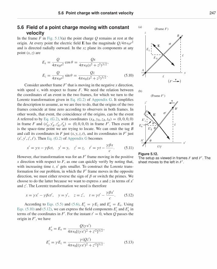
5.6 Point charge with constant velocity 247
5.6 Field of a point charge moving with constantvelocity
In the frame F in Fig. 5.13(a) the point charge Q remains at rest at theorigin. At every point the electric field E has the magnitude Q/4πε0r2
and is directed radially outward. In the xz plane its components at anypoint (x, z) are
Ex = Q4πε0r2 cos θ = Qx
4πε0(x2 + z2)3/2 ,
Ez = Q4πε0r2 sin θ = Qz
4πε0(x2 + z2)3/2 . (5.10)
q
s
x
z
A
B
E
E⊥
s'
x'
z'
A'
B'
F'
E'
E'⊥En'
/g
E
E'
(Frame F )
(Frame F' )
v
v
(a)
(b)
Figure 5.12.The setup as viewed in frames F and F′. Thesheet moves to the left in F′.
Consider another frame F′ that is moving in the negative x direction,with speed v, with respect to frame F. We need the relation betweenthe coordinates of an event in the two frames, for which we turn to theLorentz transformation given in Eq. (G.2) of Appendix G. It simplifiesthe description to assume, as we are free to do, that the origins of the twoframes coincide at time zero according to observers in both frames. Inother words, that event, the coincidence of the origins, can be the eventA referred to by Eq. (G.2), with coordinates (xA, yA, zA, tA) = (0, 0, 0, 0)
in frame F and (x′A, y′A, z′A, t′A) = (0, 0, 0, 0) in frame F′. Then event Bis the space-time point we are trying to locate. We can omit the tag Band call its coordinates in F just (x, y, z, t), and its coordinates in F′ just(x′, y′, z′, t′). Then Eq. (G.2) of Appendix G becomes
x′ = γ x − γβct, y′ = y, z′ = z, t′ = γ t − γβxc
. (5.11)
However, that transformation was for an F′ frame moving in the positivex direction with respect to F, as one can quickly verify by noting that,with increasing time t, x′ gets smaller. To construct the Lorentz trans-formation for our problem, in which the F′ frame moves in the oppositedirection, we must either reverse the sign of β or switch the primes. Wechoose to do the latter because we want to express x and z in terms of x′and z′. The Lorentz transformation we need is therefore
x = γ x′ − γβct′, y = y′, z = z′, t = γ t′ − γβx′
c. (5.12)
According to Eqs. (5.5) and (5.6), E′z = γ Ez and E′
x = Ex. UsingEqs. (5.10) and (5.12), we can express the field components E′
z and E′x in
terms of the coordinates in F′. For the instant t′ = 0, when Q passes theorigin in F′, we have
E′x = Ex = Q(γ x′)
4πε0[(γ x′)2 + z′2]3/2 ,
E′z = γ Ez = γ (Qz′)
4πε0[(γ x′)2 + z′2]3/2 . (5.13)
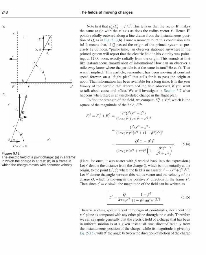
248 The fields of moving charges
Note first that E′z/E′
x = z′/x′. This tells us that the vector E′ makesthe same angle with the x′ axis as does the radius vector r′. Hence E′points radially outward along a line drawn from the instantaneous posi-tion of Q, as in Fig. 5.13(b). Pause a moment to let this conclusion sinkin! It means that, if Q passed the origin of the primed system at pre-cisely 12:00 noon, “prime time,” an observer stationed anywhere in theprimed system will report that the electric field in his vicinity was point-ing, at 12:00 noon, exactly radially from the origin. This sounds at firstlike instantaneous transmission of information! How can an observer amile away know where the particle is at the same instant? He can’t. Thatwasn’t implied. This particle, remember, has been moving at constantspeed forever, on a “flight plan” that calls for it to pass the origin atnoon. That information has been available for a long time. It is the pasthistory of the particle that determined the field observed, if you wantto talk about cause and effect. We will investigate in Section 5.7 whathappens when there is an unscheduled change in the flight plan.
F¢ F
x
x¢
Q
v
z¢z
(x, z)Ex
r
EEz
(a)
q
q¢
vQ
F¢ at t¢ = 0
x¢
r¢
z¢Ez¢
Ex¢
E¢
(b)
Figure 5.13.The electric field of a point charge: (a) in a framein which the charge is at rest; (b) in a frame inwhich the charge moves with constant velocity.
To find the strength of the field, we compute E′2x + E′2
z , which is thesquare of the magnitude of the field, E′2:
E′2 = E′2x + E′2
z = γ 2Q2(x′2 + z′2)(4πε0)2[(γ x′)2 + z′2]3
= Q2(x′2 + z′2)(4πε0)2γ 4[x′2 + (1 − β2)z′2]3
= Q2(1 − β2)2
(4πε0)2(x′2 + z′2)2(
1 − β2z′2
x′2 + z′2
)3 . (5.14)
(Here, for once, it was neater with β worked back into the expression.)Let r′ denote the distance from the charge Q, which is momentarily at theorigin, to the point (x′, z′) where the field is measured: r′ = (x′2+z′2)1/2.Let θ ′ denote the angle between this radius vector and the velocity of thecharge Q, which is moving in the positive x′ direction in the frame F′.Then since z′ = r′ sin θ ′, the magnitude of the field can be written as
E′ = Q4πε0r′2
1 − β2
(1 − β2 sin2 θ ′)3/2(5.15)
There is nothing special about the origin of coordinates, nor about thex′z′ plane as compared with any other plane through the x′ axis. Thereforewe can say quite generally that the electric field of a charge that has beenin uniform motion is at a given instant of time directed radially fromthe instantaneous position of the charge, while its magnitude is given byEq. (5.15), with θ ′ the angle between the direction of motion of the charge
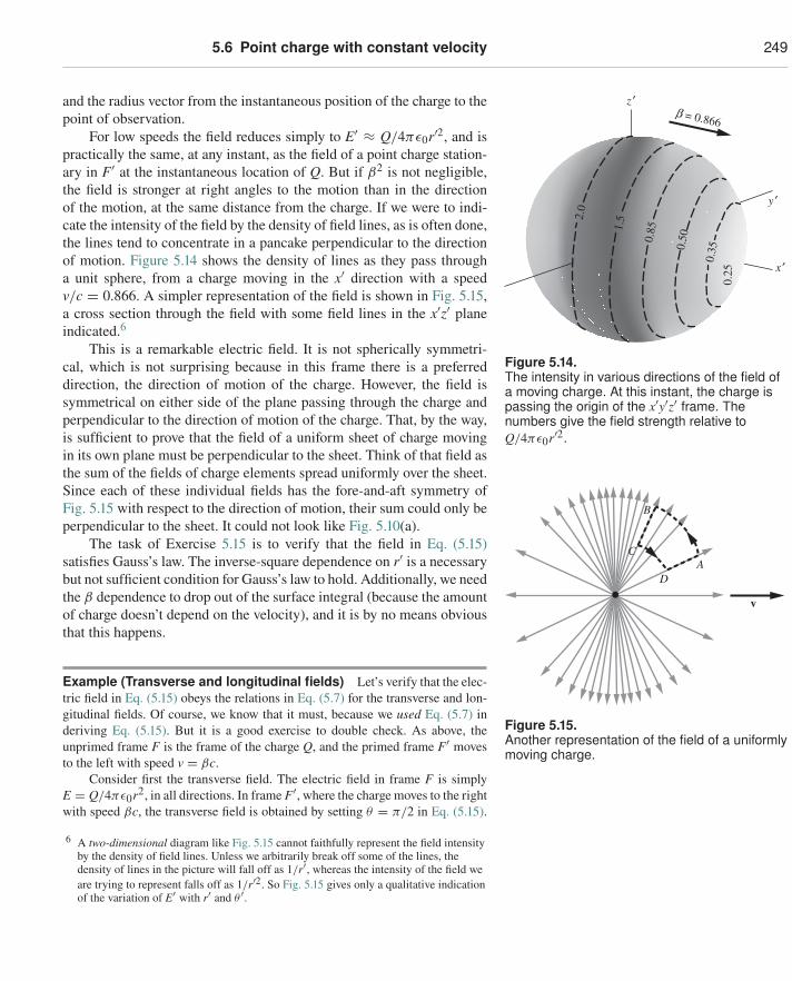
5.6 Point charge with constant velocity 249
and the radius vector from the instantaneous position of the charge to thepoint of observation.
For low speeds the field reduces simply to E′ ≈ Q/4πε0r′2, and ispractically the same, at any instant, as the field of a point charge station-ary in F′ at the instantaneous location of Q. But if β2 is not negligible,the field is stronger at right angles to the motion than in the directionof the motion, at the same distance from the charge. If we were to indi-cate the intensity of the field by the density of field lines, as is often done,the lines tend to concentrate in a pancake perpendicular to the directionof motion. Figure 5.14 shows the density of lines as they pass througha unit sphere, from a charge moving in the x′ direction with a speedv/c = 0.866. A simpler representation of the field is shown in Fig. 5.15,a cross section through the field with some field lines in the x′z′ planeindicated.6
0.25
0.350.
500.851.
52.0
x ′
y ′
z ′b = 0.866
Figure 5.14.The intensity in various directions of the field ofa moving charge. At this instant, the charge ispassing the origin of the x′y′z′ frame. Thenumbers give the field strength relative toQ/4πε0r′2.
This is a remarkable electric field. It is not spherically symmetri-cal, which is not surprising because in this frame there is a preferreddirection, the direction of motion of the charge. However, the field issymmetrical on either side of the plane passing through the charge andperpendicular to the direction of motion of the charge. That, by the way,is sufficient to prove that the field of a uniform sheet of charge movingin its own plane must be perpendicular to the sheet. Think of that field asthe sum of the fields of charge elements spread uniformly over the sheet.Since each of these individual fields has the fore-and-aft symmetry ofFig. 5.15 with respect to the direction of motion, their sum could only beperpendicular to the sheet. It could not look like Fig. 5.10(a).
B
DA
v
C
Figure 5.15.Another representation of the field of a uniformlymoving charge.
The task of Exercise 5.15 is to verify that the field in Eq. (5.15)satisfies Gauss’s law. The inverse-square dependence on r′ is a necessarybut not sufficient condition for Gauss’s law to hold. Additionally, we needthe β dependence to drop out of the surface integral (because the amountof charge doesn’t depend on the velocity), and it is by no means obviousthat this happens.
Example (Transverse and longitudinal fields) Let’s verify that the elec-tric field in Eq. (5.15) obeys the relations in Eq. (5.7) for the transverse and lon-gitudinal fields. Of course, we know that it must, because we used Eq. (5.7) inderiving Eq. (5.15). But it is a good exercise to double check. As above, theunprimed frame F is the frame of the charge Q, and the primed frame F′ movesto the left with speed v = βc.
Consider first the transverse field. The electric field in frame F is simplyE = Q/4πε0r2, in all directions. In frame F′, where the charge moves to the rightwith speed βc, the transverse field is obtained by setting θ = π/2 in Eq. (5.15).
6 A two-dimensional diagram like Fig. 5.15 cannot faithfully represent the field intensityby the density of field lines. Unless we arbitrarily break off some of the lines, thedensity of lines in the picture will fall off as 1/r′, whereas the intensity of the field weare trying to represent falls off as 1/r′2. So Fig. 5.15 gives only a qualitative indicationof the variation of E′ with r′ and θ ′.
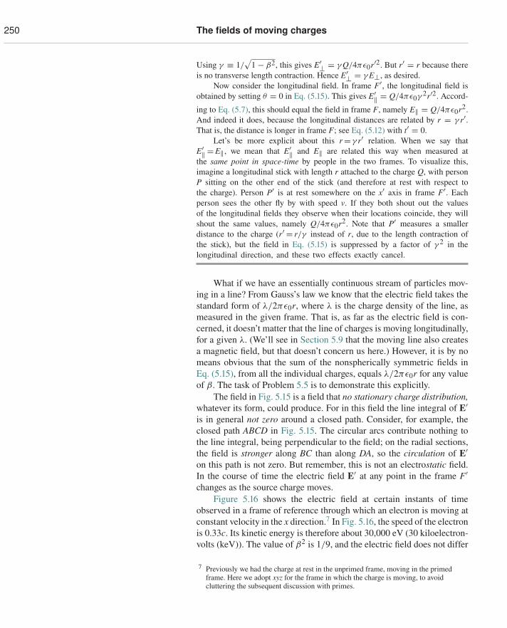
250 The fields of moving charges
Using γ ≡ 1/√
1 − β2, this gives E′⊥ = γ Q/4πε0r′2. But r′ = r because thereis no transverse length contraction. Hence E′⊥ = γ E⊥, as desired.
Now consider the longitudinal field. In frame F′, the longitudinal field isobtained by setting θ = 0 in Eq. (5.15). This gives E′‖ = Q/4πε0γ 2r′2. Accord-
ing to Eq. (5.7), this should equal the field in frame F, namely E‖ = Q/4πε0r2.And indeed it does, because the longitudinal distances are related by r = γ r′.That is, the distance is longer in frame F; see Eq. (5.12) with t′ = 0.
Let’s be more explicit about this r= γ r′ relation. When we say thatE′‖ =E‖, we mean that E′‖ and E‖ are related this way when measured atthe same point in space-time by people in the two frames. To visualize this,imagine a longitudinal stick with length r attached to the charge Q, with personP sitting on the other end of the stick (and therefore at rest with respect tothe charge). Person P′ is at rest somewhere on the x′ axis in frame F′. Eachperson sees the other fly by with speed v. If they both shout out the valuesof the longitudinal fields they observe when their locations coincide, they willshout the same values, namely Q/4πε0r2. Note that P′ measures a smallerdistance to the charge (r′ = r/γ instead of r, due to the length contraction ofthe stick), but the field in Eq. (5.15) is suppressed by a factor of γ 2 in thelongitudinal direction, and these two effects exactly cancel.
What if we have an essentially continuous stream of particles mov-ing in a line? From Gauss’s law we know that the electric field takes thestandard form of λ/2πε0r, where λ is the charge density of the line, asmeasured in the given frame. That is, as far as the electric field is con-cerned, it doesn’t matter that the line of charges is moving longitudinally,for a given λ. (We’ll see in Section 5.9 that the moving line also createsa magnetic field, but that doesn’t concern us here.) However, it is by nomeans obvious that the sum of the nonspherically symmetric fields inEq. (5.15), from all the individual charges, equals λ/2πε0r for any valueof β. The task of Problem 5.5 is to demonstrate this explicitly.
The field in Fig. 5.15 is a field that no stationary charge distribution,whatever its form, could produce. For in this field the line integral of E′is in general not zero around a closed path. Consider, for example, theclosed path ABCD in Fig. 5.15. The circular arcs contribute nothing tothe line integral, being perpendicular to the field; on the radial sections,the field is stronger along BC than along DA, so the circulation of E′on this path is not zero. But remember, this is not an electrostatic field.In the course of time the electric field E′ at any point in the frame F′changes as the source charge moves.
Figure 5.16 shows the electric field at certain instants of timeobserved in a frame of reference through which an electron is moving atconstant velocity in the x direction.7 In Fig. 5.16, the speed of the electronis 0.33c. Its kinetic energy is therefore about 30,000 eV (30 kiloelectron-volts (keV)). The value of β2 is 1/9, and the electric field does not differ
7 Previously we had the charge at rest in the unprimed frame, moving in the primedframe. Here we adopt xyz for the frame in which the charge is moving, to avoidcluttering the subsequent discussion with primes.
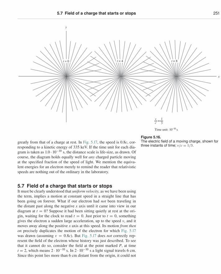
5.7 Field of a charge that starts or stops 251
x
y
Time unit: 10–10 s
= 13c
v
t = 0 t = 4 t = 8
Figure 5.16.The electric field of a moving charge, shown forthree instants of time; v/c = 1/3.
greatly from that of a charge at rest. In Fig. 5.17, the speed is 0.8c, cor-responding to a kinetic energy of 335 keV. If the time unit for each dia-gram is taken as 1.0 · 10−10 s, the distance scale is life-size, as drawn. Ofcourse, the diagram holds equally well for any charged particle movingat the specified fraction of the speed of light. We mention the equiva-lent energies for an electron merely to remind the reader that relativisticspeeds are nothing out of the ordinary in the laboratory.
5.7 Field of a charge that starts or stopsIt must be clearly understood that uniform velocity, as we have been usingthe term, implies a motion at constant speed in a straight line that hasbeen going on forever. What if our electron had not been traveling inthe distant past along the negative x axis until it came into view in ourdiagram at t = 0? Suppose it had been sitting quietly at rest at the ori-gin, waiting for the clock to read t = 0. Just prior to t = 0, somethinggives the electron a sudden large acceleration, up to the speed v, and itmoves away along the positive x axis at this speed. Its motion from thenon precisely duplicates the motion of the electron for which Fig. 5.17was drawn (assuming v = 0.8c). But Fig. 5.17 does not correctly rep-resent the field of the electron whose history was just described. To seethat it cannot do so, consider the field at the point marked P, at timet = 2, which means 2 · 10−10 s. In 2 · 10−10 s a light signal travels 6 cm.Since this point lies more than 6 cm distant from the origin, it could not
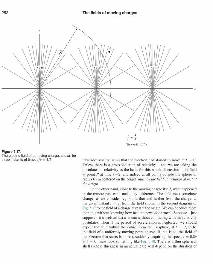
252 The fields of moving charges
Time unit: 10–10 s
P
6 cm
x
y
c45
=v
t = 0 t = 2 t = 4
Figure 5.17.The electric field of a moving charge, shown forthree instants of time; v/c = 4/5. have received the news that the electron had started to move at t = 0!
Unless there is a gross violation of relativity – and we are taking thepostulates of relativity as the basis for this whole discussion – the fieldat point P at time t= 2, and indeed at all points outside the sphere ofradius 6 cm centered on the origin, must be the field of a charge at rest atthe origin.
On the other hand, close to the moving charge itself, what happenedin the remote past can’t make any difference. The field must somehowchange, as we consider regions farther and farther from the charge, atthe given instant t = 2, from the field shown in the second diagram ofFig. 5.17 to the field of a charge at rest at the origin. We can’t deduce morethan this without knowing how fast the news does travel. Suppose – justsuppose – it travels as fast as it can without conflicting with the relativitypostulates. Then if the period of acceleration is neglected, we shouldexpect the field within the entire 6 cm radius sphere, at t = 2, to bethe field of a uniformly moving point charge. If that is so, the field ofthe electron that starts from rest, suddenly acquiring the speed v = 0.8cat t = 0, must look something like Fig. 5.18. There is a thin sphericalshell (whose thickness in an actual case will depend on the duration of
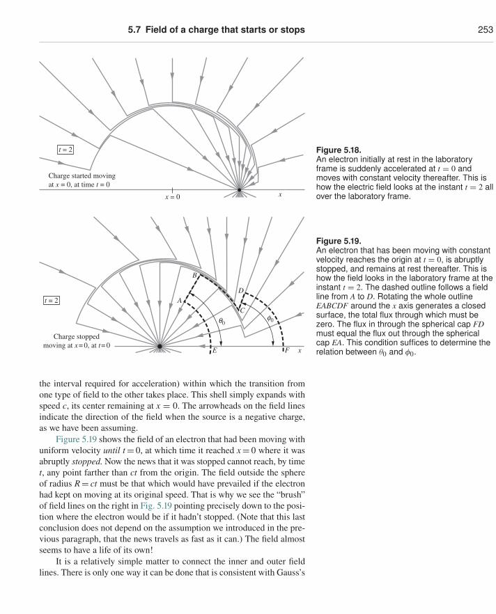
5.7 Field of a charge that starts or stops 253
Charge started movingat x = 0, at time t = 0
x = 0
t = 2
x
Figure 5.18.An electron initially at rest in the laboratoryframe is suddenly accelerated at t = 0 andmoves with constant velocity thereafter. This ishow the electric field looks at the instant t = 2 allover the laboratory frame.
Charge stoppedmoving at x= 0, at t= 0
E F
D
C
B
A
x
q0f0
t = 2
Figure 5.19.An electron that has been moving with constantvelocity reaches the origin at t = 0, is abruptlystopped, and remains at rest thereafter. This ishow the field looks in the laboratory frame at theinstant t = 2. The dashed outline follows a fieldline from A to D. Rotating the whole outlineEABCDF around the x axis generates a closedsurface, the total flux through which must bezero. The flux in through the spherical cap FDmust equal the flux out through the sphericalcap EA. This condition suffices to determine therelation between θ0 and φ0.
the interval required for acceleration) within which the transition fromone type of field to the other takes place. This shell simply expands withspeed c, its center remaining at x = 0. The arrowheads on the field linesindicate the direction of the field when the source is a negative charge,as we have been assuming.
Figure 5.19 shows the field of an electron that had been moving withuniform velocity until t= 0, at which time it reached x= 0 where it wasabruptly stopped. Now the news that it was stopped cannot reach, by timet, any point farther than ct from the origin. The field outside the sphereof radius R= ct must be that which would have prevailed if the electronhad kept on moving at its original speed. That is why we see the “brush”of field lines on the right in Fig. 5.19 pointing precisely down to the posi-tion where the electron would be if it hadn’t stopped. (Note that this lastconclusion does not depend on the assumption we introduced in the pre-vious paragraph, that the news travels as fast as it can.) The field almostseems to have a life of its own!
It is a relatively simple matter to connect the inner and outer fieldlines. There is only one way it can be done that is consistent with Gauss’s
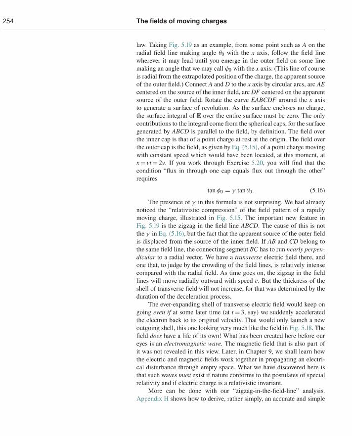
254 The fields of moving charges
law. Taking Fig. 5.19 as an example, from some point such as A on theradial field line making angle θ0 with the x axis, follow the field linewherever it may lead until you emerge in the outer field on some linemaking an angle that we may call φ0 with the x axis. (This line of courseis radial from the extrapolated position of the charge, the apparent sourceof the outer field.) Connect A and D to the x axis by circular arcs, arc AEcentered on the source of the inner field, arc DF centered on the apparentsource of the outer field. Rotate the curve EABCDF around the x axisto generate a surface of revolution. As the surface encloses no charge,the surface integral of E over the entire surface must be zero. The onlycontributions to the integral come from the spherical caps, for the surfacegenerated by ABCD is parallel to the field, by definition. The field overthe inner cap is that of a point charge at rest at the origin. The field overthe outer cap is the field, as given by Eq. (5.15), of a point charge movingwith constant speed which would have been located, at this moment, atx= vt= 2v. If you work through Exercise 5.20, you will find that thecondition “flux in through one cap equals flux out through the other”requires
tan φ0 = γ tan θ0. (5.16)
The presence of γ in this formula is not surprising. We had alreadynoticed the “relativistic compression” of the field pattern of a rapidlymoving charge, illustrated in Fig. 5.15. The important new feature inFig. 5.19 is the zigzag in the field line ABCD. The cause of this is notthe γ in Eq. (5.16), but the fact that the apparent source of the outer fieldis displaced from the source of the inner field. If AB and CD belong tothe same field line, the connecting segment BC has to run nearly perpen-dicular to a radial vector. We have a transverse electric field there, andone that, to judge by the crowding of the field lines, is relatively intensecompared with the radial field. As time goes on, the zigzag in the fieldlines will move radially outward with speed c. But the thickness of theshell of transverse field will not increase, for that was determined by theduration of the deceleration process.
The ever-expanding shell of transverse electric field would keep ongoing even if at some later time (at t= 3, say) we suddenly acceleratedthe electron back to its original velocity. That would only launch a newoutgoing shell, this one looking very much like the field in Fig. 5.18. Thefield does have a life of its own! What has been created here before oureyes is an electromagnetic wave. The magnetic field that is also part ofit was not revealed in this view. Later, in Chapter 9, we shall learn howthe electric and magnetic fields work together in propagating an electri-cal disturbance through empty space. What we have discovered here isthat such waves must exist if nature conforms to the postulates of specialrelativity and if electric charge is a relativistic invariant.
More can be done with our “zigzag-in-the-field-line” analysis.Appendix H shows how to derive, rather simply, an accurate and simple
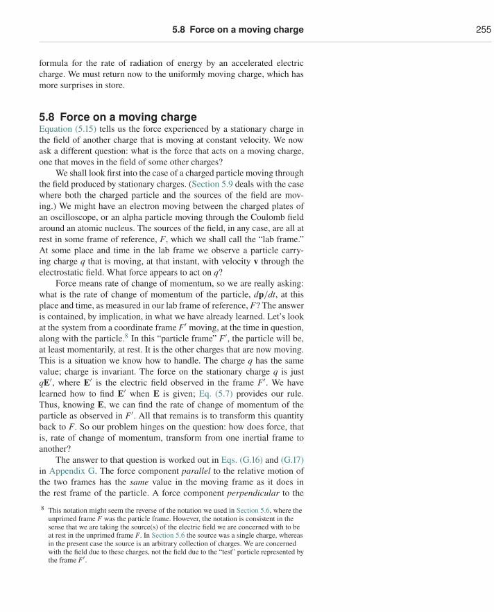
5.8 Force on a moving charge 255
formula for the rate of radiation of energy by an accelerated electriccharge. We must return now to the uniformly moving charge, which hasmore surprises in store.
5.8 Force on a moving chargeEquation (5.15) tells us the force experienced by a stationary charge inthe field of another charge that is moving at constant velocity. We nowask a different question: what is the force that acts on a moving charge,one that moves in the field of some other charges?
We shall look first into the case of a charged particle moving throughthe field produced by stationary charges. (Section 5.9 deals with the casewhere both the charged particle and the sources of the field are mov-ing.) We might have an electron moving between the charged plates ofan oscilloscope, or an alpha particle moving through the Coulomb fieldaround an atomic nucleus. The sources of the field, in any case, are all atrest in some frame of reference, F, which we shall call the “lab frame.”At some place and time in the lab frame we observe a particle carry-ing charge q that is moving, at that instant, with velocity v through theelectrostatic field. What force appears to act on q?
Force means rate of change of momentum, so we are really asking:what is the rate of change of momentum of the particle, dp/dt, at thisplace and time, as measured in our lab frame of reference, F? The answeris contained, by implication, in what we have already learned. Let’s lookat the system from a coordinate frame F′ moving, at the time in question,along with the particle.8 In this “particle frame” F′, the particle will be,at least momentarily, at rest. It is the other charges that are now moving.This is a situation we know how to handle. The charge q has the samevalue; charge is invariant. The force on the stationary charge q is justqE′, where E′ is the electric field observed in the frame F′. We havelearned how to find E′ when E is given; Eq. (5.7) provides our rule.Thus, knowing E, we can find the rate of change of momentum of theparticle as observed in F′. All that remains is to transform this quantityback to F. So our problem hinges on the question: how does force, thatis, rate of change of momentum, transform from one inertial frame toanother?
The answer to that question is worked out in Eqs. (G.16) and (G.17)in Appendix G. The force component parallel to the relative motion ofthe two frames has the same value in the moving frame as it does inthe rest frame of the particle. A force component perpendicular to the
8 This notation might seem the reverse of the notation we used in Section 5.6, where theunprimed frame F was the particle frame. However, the notation is consistent in thesense that we are taking the source(s) of the electric field we are concerned with to beat rest in the unprimed frame F. In Section 5.6 the source was a single charge, whereasin the present case the source is an arbitrary collection of charges. We are concernedwith the field due to these charges, not the field due to the “test” particle represented bythe frame F′.
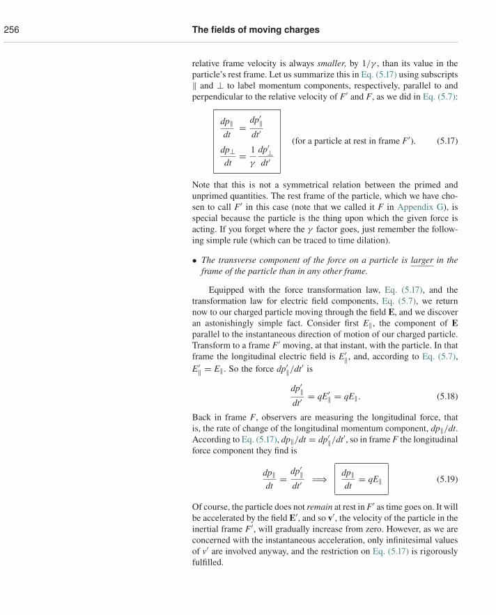
256 The fields of moving charges
relative frame velocity is always smaller, by 1/γ , than its value in theparticle’s rest frame. Let us summarize this in Eq. (5.17) using subscripts‖ and ⊥ to label momentum components, respectively, parallel to andperpendicular to the relative velocity of F′ and F, as we did in Eq. (5.7):
dp‖dt
= dp′‖dt′
dp⊥dt
= 1γ
dp′⊥dt′
(for a particle at rest in frame F′). (5.17)
Note that this is not a symmetrical relation between the primed andunprimed quantities. The rest frame of the particle, which we have cho-sen to call F′ in this case (note that we called it F in Appendix G), isspecial because the particle is the thing upon which the given force isacting. If you forget where the γ factor goes, just remember the follow-ing simple rule (which can be traced to time dilation).
• The transverse component of the force on a particle is larger in theframe of the particle than in any other frame.
Equipped with the force transformation law, Eq. (5.17), and thetransformation law for electric field components, Eq. (5.7), we returnnow to our charged particle moving through the field E, and we discoveran astonishingly simple fact. Consider first E‖, the component of Eparallel to the instantaneous direction of motion of our charged particle.Transform to a frame F′ moving, at that instant, with the particle. In thatframe the longitudinal electric field is E′‖, and, according to Eq. (5.7),E′‖ = E‖. So the force dp′‖/dt′ is
dp′‖dt′
= qE′‖ = qE‖. (5.18)
Back in frame F, observers are measuring the longitudinal force, thatis, the rate of change of the longitudinal momentum component, dp‖/dt.According to Eq. (5.17), dp‖/dt = dp′‖/dt′, so in frame F the longitudinalforce component they find is
dp‖dt
= dp′‖dt′
�⇒ dp‖dt
= qE‖ (5.19)
Of course, the particle does not remain at rest in F′ as time goes on. It willbe accelerated by the field E′, and so v′, the velocity of the particle in theinertial frame F′, will gradually increase from zero. However, as we areconcerned with the instantaneous acceleration, only infinitesimal valuesof v′ are involved anyway, and the restriction on Eq. (5.17) is rigorouslyfulfilled.
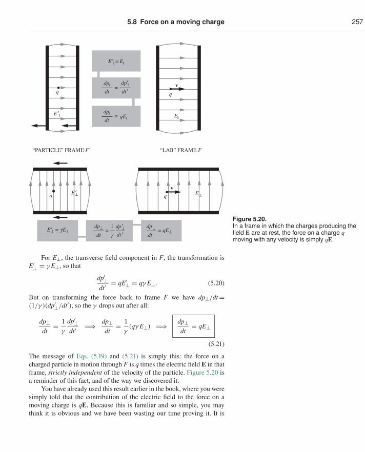
5.8 Force on a moving charge 257
q q
E ′|| E||
E ′|| = E||
qE||
dp||
dt
dp|| dp′||dt dt ′
=
=
“PARTICLE” FRAME F ′ “LAB” FRAME F
q E ′⊥ qv
v
E ′⊥ = gE⊥ gdp⊥ dp ′⊥ dp⊥ qE⊥dt dt ′ dt
=1
=
E⊥
Figure 5.20.In a frame in which the charges producing thefield E are at rest, the force on a charge qmoving with any velocity is simply qE.
For E⊥, the transverse field component in F, the transformation isE′⊥ = γ E⊥, so that
dp′⊥dt′
= qE′⊥ = qγ E⊥. (5.20)
But on transforming the force back to frame F we have dp⊥/dt=(1/γ )(dp′⊥/dt′), so the γ drops out after all:
dp⊥dt
= 1γ
dp′⊥dt′
�⇒ dp⊥dt
= 1γ
(qγ E⊥) �⇒ dp⊥dt
= qE⊥
(5.21)
The message of Eqs. (5.19) and (5.21) is simply this: the force on acharged particle in motion through F is q times the electric field E in thatframe, strictly independent of the velocity of the particle. Figure 5.20 isa reminder of this fact, and of the way we discovered it.
You have already used this result earlier in the book, where you weresimply told that the contribution of the electric field to the force on amoving charge is qE. Because this is familiar and so simple, you maythink it is obvious and we have been wasting our time proving it. It is
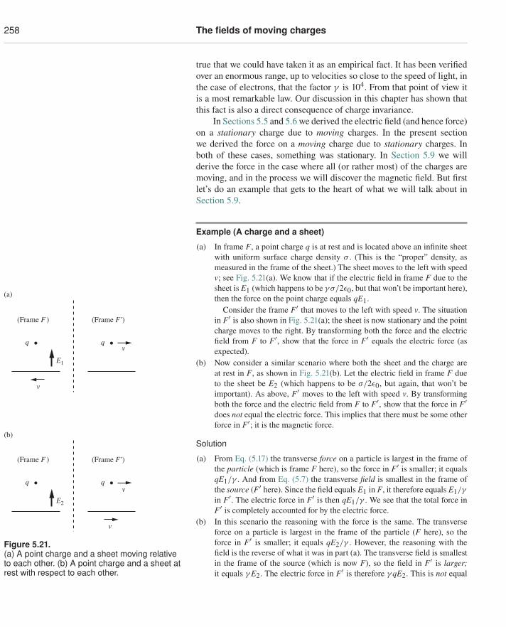
258 The fields of moving charges
true that we could have taken it as an empirical fact. It has been verifiedover an enormous range, up to velocities so close to the speed of light, inthe case of electrons, that the factor γ is 104. From that point of view itis a most remarkable law. Our discussion in this chapter has shown thatthis fact is also a direct consequence of charge invariance.
In Sections 5.5 and 5.6 we derived the electric field (and hence force)on a stationary charge due to moving charges. In the present sectionwe derived the force on a moving charge due to stationary charges. Inboth of these cases, something was stationary. In Section 5.9 we willderive the force in the case where all (or rather most) of the charges aremoving, and in the process we will discover the magnetic field. But firstlet’s do an example that gets to the heart of what we will talk about inSection 5.9.
Example (A charge and a sheet)
(a) In frame F, a point charge q is at rest and is located above an infinite sheetwith uniform surface charge density σ . (This is the “proper” density, asmeasured in the frame of the sheet.) The sheet moves to the left with speedv; see Fig. 5.21(a). We know that if the electric field in frame F due to the
v
q
(a)
(b)
E1
(Frame F )
vq
(Frame F' )
q
(Frame F )
vq
v
(Frame F' )
E2
Figure 5.21.(a) A point charge and a sheet moving relativeto each other. (b) A point charge and a sheet atrest with respect to each other.
sheet is E1 (which happens to be γ σ/2ε0, but that won’t be important here),then the force on the point charge equals qE1.
Consider the frame F′ that moves to the left with speed v. The situationin F′ is also shown in Fig. 5.21(a); the sheet is now stationary and the pointcharge moves to the right. By transforming both the force and the electricfield from F to F′, show that the force in F′ equals the electric force (asexpected).
(b) Now consider a similar scenario where both the sheet and the charge areat rest in F, as shown in Fig. 5.21(b). Let the electric field in frame F dueto the sheet be E2 (which happens to be σ/2ε0, but again, that won’t beimportant). As above, F′ moves to the left with speed v. By transformingboth the force and the electric field from F to F′, show that the force in F′does not equal the electric force. This implies that there must be some otherforce in F′; it is the magnetic force.
Solution
(a) From Eq. (5.17) the transverse force on a particle is largest in the frame ofthe particle (which is frame F here), so the force in F′ is smaller; it equalsqE1/γ . And from Eq. (5.7) the transverse field is smallest in the frame ofthe source (F′ here). Since the field equals E1 in F, it therefore equals E1/γ
in F′. The electric force in F′ is then qE1/γ . We see that the total force inF′ is completely accounted for by the electric force.
(b) In this scenario the reasoning with the force is the same. The transverseforce on a particle is largest in the frame of the particle (F here), so theforce in F′ is smaller; it equals qE2/γ . However, the reasoning with thefield is the reverse of what it was in part (a). The transverse field is smallestin the frame of the source (which is now F), so the field in F′ is larger;it equals γ E2. The electric force in F′ is therefore γ qE2. This is not equal
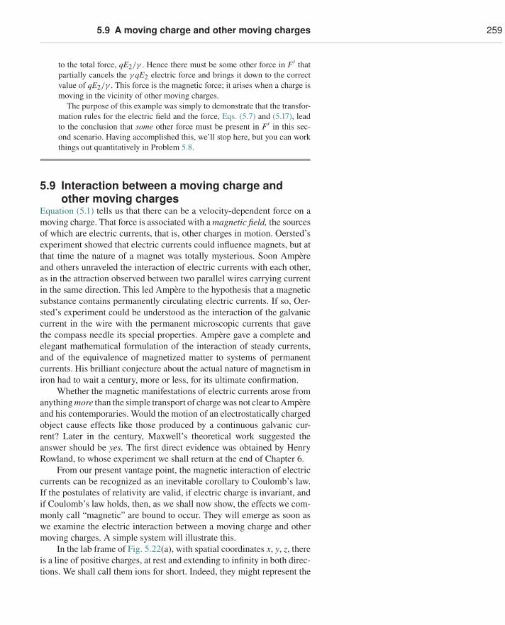
5.9 A moving charge and other moving charges 259
to the total force, qE2/γ . Hence there must be some other force in F′ thatpartially cancels the γ qE2 electric force and brings it down to the correctvalue of qE2/γ . This force is the magnetic force; it arises when a charge ismoving in the vicinity of other moving charges.
The purpose of this example was simply to demonstrate that the transfor-mation rules for the electric field and the force, Eqs. (5.7) and (5.17), leadto the conclusion that some other force must be present in F′ in this sec-ond scenario. Having accomplished this, we’ll stop here, but you can workthings out quantitatively in Problem 5.8.
5.9 Interaction between a moving charge andother moving charges
Equation (5.1) tells us that there can be a velocity-dependent force on amoving charge. That force is associated with a magnetic field, the sourcesof which are electric currents, that is, other charges in motion. Oersted’sexperiment showed that electric currents could influence magnets, but atthat time the nature of a magnet was totally mysterious. Soon Ampèreand others unraveled the interaction of electric currents with each other,as in the attraction observed between two parallel wires carrying currentin the same direction. This led Ampère to the hypothesis that a magneticsubstance contains permanently circulating electric currents. If so, Oer-sted’s experiment could be understood as the interaction of the galvaniccurrent in the wire with the permanent microscopic currents that gavethe compass needle its special properties. Ampère gave a complete andelegant mathematical formulation of the interaction of steady currents,and of the equivalence of magnetized matter to systems of permanentcurrents. His brilliant conjecture about the actual nature of magnetism iniron had to wait a century, more or less, for its ultimate confirmation.
Whether the magnetic manifestations of electric currents arose fromanything more than the simple transport of charge was not clear to Ampèreand his contemporaries. Would the motion of an electrostatically chargedobject cause effects like those produced by a continuous galvanic cur-rent? Later in the century, Maxwell’s theoretical work suggested theanswer should be yes. The first direct evidence was obtained by HenryRowland, to whose experiment we shall return at the end of Chapter 6.
From our present vantage point, the magnetic interaction of electriccurrents can be recognized as an inevitable corollary to Coulomb’s law.If the postulates of relativity are valid, if electric charge is invariant, andif Coulomb’s law holds, then, as we shall now show, the effects we com-monly call “magnetic” are bound to occur. They will emerge as soon aswe examine the electric interaction between a moving charge and othermoving charges. A simple system will illustrate this.
In the lab frame of Fig. 5.22(a), with spatial coordinates x, y, z, thereis a line of positive charges, at rest and extending to infinity in both direc-tions. We shall call them ions for short. Indeed, they might represent the
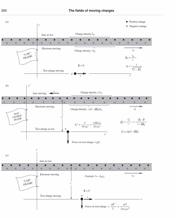
260 The fields of moving charges
‘‘LAB’’
FRAME
Ions at rest
Electrons movingCharge density −λ0
Test charge moving
E = 0
x
y
qv
v0
g0
v0b0
Charge density λ0
Positive charge
Negative charge
=
=
c
1
1 − b 20
(a)
Ions moving
Electrons moving
TEST
CHARGE
FRAME
Test charge at rest
Charge density g λ0
Charge density −g (1 − bb0)λ0
Force on test charge = qEr′
y¢
v
(b)
r¢
q
v0¢
v0¢
x¢
b¢0b0 − b
c 1 − bb0=
g ¢0 gg0(1 – bb0)=
=Er =
λ
2 0r= γββ0λ0
2 0r
Ions at rest
y
x
Electrons movingCurrent: I = –λ0v0
v
E = 0
Force on test charge
q
qE ′ qvI
g
Test charge moving
“LAB”
FRAME
v0
(c)
==
r
2 0rc2
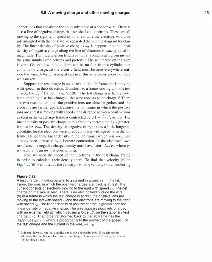
5.9 A moving charge and other moving charges 261
copper ions that constitute the solid substance of a copper wire. There isalso a line of negative charges that we shall call electrons. These are allmoving to the right with speed v0. In a real wire the electrons would beintermingled with the ions; we’ve separated them in the diagram for clar-ity. The linear density of positive charge is λ0. It happens that the lineardensity of negative charge along the line of electrons is exactly equal inmagnitude. That is, any given length of “wire” contains at a given instantthe same number of electrons and protons.9 The net charge on the wireis zero. Gauss’s law tells us there can be no flux from a cylinder thatcontains no charge, so the electric field must be zero everywhere out-side the wire. A test charge q at rest near this wire experiences no forcewhatsoever.
Suppose the test charge is not at rest in the lab frame but is movingwith speed v in the x direction. Transform to a frame moving with the testcharge, the x′, y′ frame in Fig. 5.22(b). The test charge q is here at rest,but something else has changed: the wire appears to be charged! Thereare two reasons for that: the positive ions are closer together, and theelectrons are farther apart. Because the lab frame in which the positiveions are at rest is moving with speed v, the distance between positive ionsas seen in the test charge frame is contracted by
√1 − v2/c2, or 1/γ . The
linear density of positive charge in this frame is correspondingly greater;it must be γ λ0. The density of negative charge takes a little longer tocalculate, for the electrons were already moving with speed v0 in the labframe. Hence their linear density in the lab frame, which was −λ0, hadalready been increased by a Lorentz contraction. In the electrons’ ownrest frame the negative charge density must have been −λ0/γ0, where γ0is the Lorentz factor that goes with v0.
Now we need the speed of the electrons in the test charge framein order to calculate their density there. To find that velocity (v′0 inFig. 5.22(b)) we must add the velocity−v to the velocity v0, remembering
Figure 5.22.A test charge q moving parallel to a current in a wire. (a) In the labframe, the wire, in which the positive charges are fixed, is at rest. Thecurrent consists of electrons moving to the right with speed v0. The netcharge on the wire is zero. There is no electric field outside the wire.(b) In a frame in which the test charge is at rest, the positive ions aremoving to the left with speed v, and the electrons are moving to the rightwith speed v′0. The linear density of positive charge is greater than thelinear density of negative charge. The wire appears positively charged,with an external field E′
r, which causes a force qE′r on the stationary test
charge q. (c) That force transformed back to the lab frame has themagnitude qE′
r/γ , which is proportional to the product of the speed v ofthe test charge and the current in the wire, −λ0v0.
9 It doesn’t have to, but that equality can always be established, if we choose, byadjusting the number of electrons per unit length. In our idealized setup, we assumethis has been done.
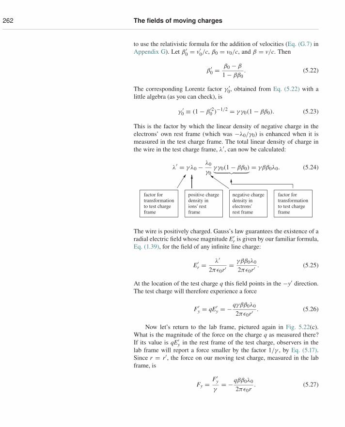
262 The fields of moving charges
to use the relativistic formula for the addition of velocities (Eq. (G.7) inAppendix G). Let β ′
0 = v′0/c, β0 = v0/c, and β = v/c. Then
β ′0 = β0 − β
1 − ββ0. (5.22)
The corresponding Lorentz factor γ ′0, obtained from Eq. (5.22) with a
little algebra (as you can check), is
γ ′0 ≡ (1 − β ′2
0 )−1/2 = γ γ0(1 − ββ0). (5.23)
This is the factor by which the linear density of negative charge in theelectrons’ own rest frame (which was −λ0/γ0) is enhanced when it ismeasured in the test charge frame. The total linear density of charge inthe wire in the test charge frame, λ′, can now be calculated:
λ′ = γ λ0 − λ0
γ0γ γ0(1 − ββ0)︸ ︷︷ ︸ = γββ0λ0. (5.24)
factor fortransformationto test chargeframe
factor fortransformationto test chargeframe
positive chargedensity inions' restframe
negative chargedensity inelectrons' rest frame
The wire is positively charged. Gauss’s law guarantees the existence of aradial electric field whose magnitude E′
r is given by our familiar formula,Eq. (1.39), for the field of any infinite line charge:
E′r =
λ′
2πε0r′= γββ0λ0
2πε0r′. (5.25)
At the location of the test charge q this field points in the −y′ direction.The test charge will therefore experience a force
F′y = qE′
y = −qγββ0λ0
2πε0r′. (5.26)
Now let’s return to the lab frame, pictured again in Fig. 5.22(c).What is the magnitude of the force on the charge q as measured there?If its value is qE′
y in the rest frame of the test charge, observers in thelab frame will report a force smaller by the factor 1/γ , by Eq. (5.17).Since r = r′, the force on our moving test charge, measured in the labframe, is
Fy =F′
y
γ= −qββ0λ0
2πε0r. (5.27)
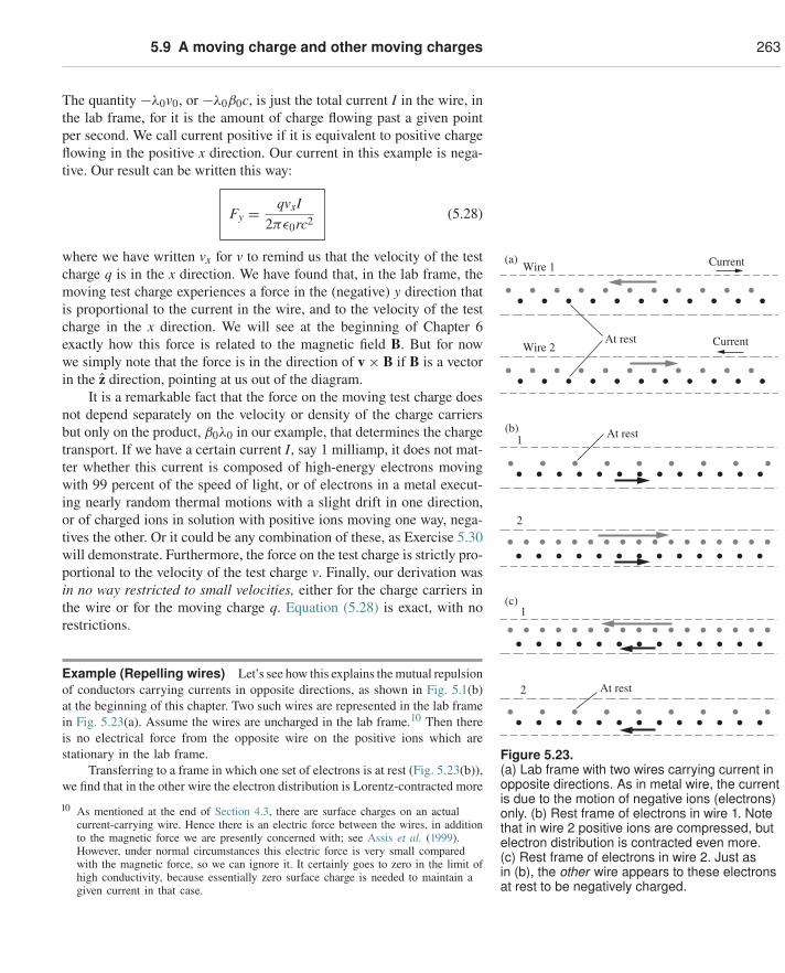
5.9 A moving charge and other moving charges 263
The quantity −λ0v0, or −λ0β0c, is just the total current I in the wire, inthe lab frame, for it is the amount of charge flowing past a given pointper second. We call current positive if it is equivalent to positive chargeflowing in the positive x direction. Our current in this example is nega-tive. Our result can be written this way:
Fy = qvxI2πε0rc2 (5.28)
where we have written vx for v to remind us that the velocity of the testcharge q is in the x direction. We have found that, in the lab frame, themoving test charge experiences a force in the (negative) y direction thatis proportional to the current in the wire, and to the velocity of the testcharge in the x direction. We will see at the beginning of Chapter 6exactly how this force is related to the magnetic field B. But for nowwe simply note that the force is in the direction of v × B if B is a vectorin the z direction, pointing at us out of the diagram.
Wire 1(a)
Wire 2At rest Current
Current
1(b)
2
At rest
At rest
1(c)
2
Figure 5.23.(a) Lab frame with two wires carrying current inopposite directions. As in metal wire, the currentis due to the motion of negative ions (electrons)only. (b) Rest frame of electrons in wire 1. Notethat in wire 2 positive ions are compressed, butelectron distribution is contracted even more.(c) Rest frame of electrons in wire 2. Just asin (b), the other wire appears to these electronsat rest to be negatively charged.
It is a remarkable fact that the force on the moving test charge doesnot depend separately on the velocity or density of the charge carriersbut only on the product, β0λ0 in our example, that determines the chargetransport. If we have a certain current I, say 1 milliamp, it does not mat-ter whether this current is composed of high-energy electrons movingwith 99 percent of the speed of light, or of electrons in a metal execut-ing nearly random thermal motions with a slight drift in one direction,or of charged ions in solution with positive ions moving one way, nega-tives the other. Or it could be any combination of these, as Exercise 5.30will demonstrate. Furthermore, the force on the test charge is strictly pro-portional to the velocity of the test charge v. Finally, our derivation wasin no way restricted to small velocities, either for the charge carriers inthe wire or for the moving charge q. Equation (5.28) is exact, with norestrictions.
Example (Repelling wires) Let’s see how this explains the mutual repulsionof conductors carrying currents in opposite directions, as shown in Fig. 5.1(b)at the beginning of this chapter. Two such wires are represented in the lab framein Fig. 5.23(a). Assume the wires are uncharged in the lab frame.10 Then thereis no electrical force from the opposite wire on the positive ions which arestationary in the lab frame.
Transferring to a frame in which one set of electrons is at rest (Fig. 5.23(b)),we find that in the other wire the electron distribution is Lorentz-contracted more
10 As mentioned at the end of Section 4.3, there are surface charges on an actualcurrent-carrying wire. Hence there is an electric force between the wires, in additionto the magnetic force we are presently concerned with; see Assis et al. (1999).However, under normal circumstances this electric force is very small comparedwith the magnetic force, so we can ignore it. It certainly goes to zero in the limit ofhigh conductivity, because essentially zero surface charge is needed to maintain agiven current in that case.
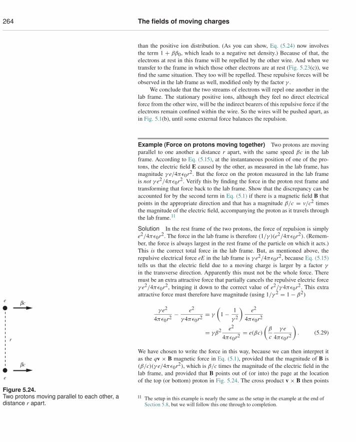
264 The fields of moving charges
than the positive ion distribution. (As you can show, Eq. (5.24) now involvesthe term 1 + ββ0, which leads to a negative net density.) Because of that, theelectrons at rest in this frame will be repelled by the other wire. And when wetransfer to the frame in which those other electrons are at rest (Fig. 5.23(c)), wefind the same situation. They too will be repelled. These repulsive forces will beobserved in the lab frame as well, modified only by the factor γ .
We conclude that the two streams of electrons will repel one another in thelab frame. The stationary positive ions, although they feel no direct electricalforce from the other wire, will be the indirect bearers of this repulsive force if theelectrons remain confined within the wire. So the wires will be pushed apart, asin Fig. 5.1(b), until some external force balances the repulsion.
Example (Force on protons moving together) Two protons are movingparallel to one another a distance r apart, with the same speed βc in the labframe. According to Eq. (5.15), at the instantaneous position of one of the pro-tons, the electric field E caused by the other, as measured in the lab frame, hasmagnitude γ e/4πε0r2. But the force on the proton measured in the lab frameis not γ e2/4πε0r2. Verify this by finding the force in the proton rest frame andtransforming that force back to the lab frame. Show that the discrepancy can beaccounted for by the second term in Eq. (5.1) if there is a magnetic field B thatpoints in the appropriate direction and that has a magnitude β/c = v/c2 timesthe magnitude of the electric field, accompanying the proton as it travels throughthe lab frame.11
bc
bc
r
e
e
Figure 5.24.Two protons moving parallel to each other, adistance r apart.
Solution In the rest frame of the two protons, the force of repulsion is simplye2/4πε0r2. The force in the lab frame is therefore (1/γ )(e2/4πε0r2). (Remem-ber, the force is always largest in the rest frame of the particle on which it acts.)This is the correct total force in the lab frame. But, as mentioned above, therepulsive electrical force eE in the lab frame is γ e2/4πε0r2, because Eq. (5.15)tells us that the electric field due to a moving charge is larger by a factor γ
in the transverse direction. Apparently this must not be the whole force. Theremust be an extra attractive force that partially cancels the repulsive electric forceγ e2/4πε0r2, bringing it down to the correct value of e2/γ 4πε0r2. This extraattractive force must therefore have magnitude (using 1/γ 2 = 1 − β2)
γ e2
4πε0r2 − e2
γ 4πε0r2 = γ
(1 − 1
γ 2
)e2
4πε0r2
= γβ2 e2
4πε0r2 = e(βc)(
β
cγ e
4πε0r2
). (5.29)
We have chosen to write the force in this way, because we can then interpret itas the qv × B magnetic force in Eq. (5.1), provided that the magnitude of B is(β/c)(γ e/4πε0r2), which is β/c times the magnitude of the electric field in thelab frame, and provided that B points out of (or into) the page at the locationof the top (or bottom) proton in Fig. 5.24. The cross product v × B then points
11 The setup in this example is nearly the same as the setup in the example at the end ofSection 5.8, but we will follow this one through to completion.
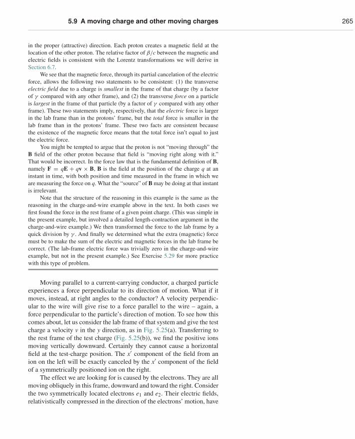
5.9 A moving charge and other moving charges 265
in the proper (attractive) direction. Each proton creates a magnetic field at thelocation of the other proton. The relative factor of β/c between the magnetic andelectric fields is consistent with the Lorentz transformations we will derive inSection 6.7.
We see that the magnetic force, through its partial cancelation of the electricforce, allows the following two statements to be consistent: (1) the transverseelectric field due to a charge is smallest in the frame of that charge (by a factorof γ compared with any other frame), and (2) the transverse force on a particleis largest in the frame of that particle (by a factor of γ compared with any otherframe). These two statements imply, respectively, that the electric force is largerin the lab frame than in the protons’ frame, but the total force is smaller in thelab frame than in the protons’ frame. These two facts are consistent becausethe existence of the magnetic force means that the total force isn’t equal to justthe electric force.
You might be tempted to argue that the proton is not “moving through” theB field of the other proton because that field is “moving right along with it.”That would be incorrect. In the force law that is the fundamental definition of B,namely F = qE + qv × B, B is the field at the position of the charge q at aninstant in time, with both position and time measured in the frame in which weare measuring the force on q. What the “source” of B may be doing at that instantis irrelevant.
Note that the structure of the reasoning in this example is the same as thereasoning in the charge-and-wire example above in the text. In both cases wefirst found the force in the rest frame of a given point charge. (This was simple inthe present example, but involved a detailed length-contraction argument in thecharge-and-wire example.) We then transformed the force to the lab frame by aquick division by γ . And finally we determined what the extra (magnetic) forcemust be to make the sum of the electric and magnetic forces in the lab frame becorrect. (The lab-frame electric force was trivially zero in the charge-and-wireexample, but not in the present example.) See Exercise 5.29 for more practicewith this type of problem.
Moving parallel to a current-carrying conductor, a charged particleexperiences a force perpendicular to its direction of motion. What if itmoves, instead, at right angles to the conductor? A velocity perpendic-ular to the wire will give rise to a force parallel to the wire – again, aforce perpendicular to the particle’s direction of motion. To see how thiscomes about, let us consider the lab frame of that system and give the testcharge a velocity v in the y direction, as in Fig. 5.25(a). Transferring tothe rest frame of the test charge (Fig. 5.25(b)), we find the positive ionsmoving vertically downward. Certainly they cannot cause a horizontalfield at the test-charge position. The x′ component of the field from anion on the left will be exactly canceled by the x′ component of the fieldof a symmetrically positioned ion on the right.
The effect we are looking for is caused by the electrons. They are allmoving obliquely in this frame, downward and toward the right. Considerthe two symmetrically located electrons e1 and e2. Their electric fields,relativistically compressed in the direction of the electrons’ motion, have
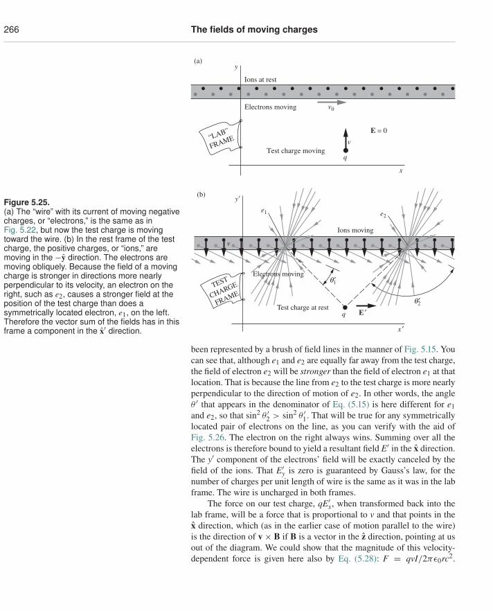
266 The fields of moving charges
Figure 5.25.(a) The “wire” with its current of moving negativecharges, or “electrons,” is the same as inFig. 5.22, but now the test charge is movingtoward the wire. (b) In the rest frame of the testcharge, the positive charges, or “ions,” aremoving in the −y direction. The electrons aremoving obliquely. Because the field of a movingcharge is stronger in directions more nearlyperpendicular to its velocity, an electron on theright, such as e2, causes a stronger field at theposition of the test charge than does asymmetrically located electron, e1, on the left.Therefore the vector sum of the fields has in thisframe a component in the x′ direction.
Ions at rest
(a)
Electrons moving
Test charge moving
E = 0
x
y
q
v0
v“LAB”
FRAME
x ′
e2
E ′qTest charge at rest
Ions moving
(b)
e1
y�
q1′
q2′
TEST
CHARGE
FRAME
Electrons moving
v
been represented by a brush of field lines in the manner of Fig. 5.15. Youcan see that, although e1 and e2 are equally far away from the test charge,the field of electron e2 will be stronger than the field of electron e1 at thatlocation. That is because the line from e2 to the test charge is more nearlyperpendicular to the direction of motion of e2. In other words, the angleθ ′ that appears in the denominator of Eq. (5.15) is here different for e1and e2, so that sin2 θ ′2 > sin2 θ ′1. That will be true for any symmetricallylocated pair of electrons on the line, as you can verify with the aid ofFig. 5.26. The electron on the right always wins. Summing over all theelectrons is therefore bound to yield a resultant field E′ in the x direction.The y′ component of the electrons’ field will be exactly canceled by thefield of the ions. That E′
y is zero is guaranteed by Gauss’s law, for thenumber of charges per unit length of wire is the same as it was in the labframe. The wire is uncharged in both frames.
The force on our test charge, qE′x, when transformed back into the
lab frame, will be a force that is proportional to v and that points in thex direction, which (as in the earlier case of motion parallel to the wire)is the direction of v × B if B is a vector in the z direction, pointing at usout of the diagram. We could show that the magnitude of this velocity-dependent force is given here also by Eq. (5.28): F = qvI/2πε0rc2.
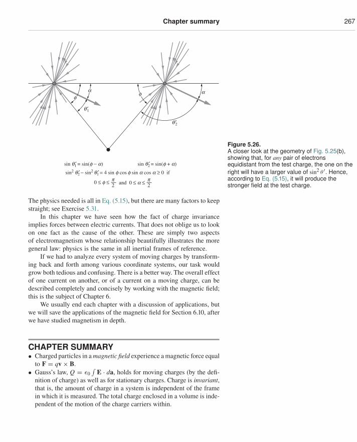
Chapter summary 267
q ′1
a
q ′2
sin q¢1 = sin(f − a) sin q¢2 = sin(f + a)
sin2 q¢2 − sin2 q¢1 = 4 sin f cos f sin a cos a ≥ 0 if
0 ≤ f ≤ 2p
2pand 0 ≤ a ≤
af
f
Figure 5.26.A closer look at the geometry of Fig. 5.25(b),showing that, for any pair of electronsequidistant from the test charge, the one on theright will have a larger value of sin2 θ ′. Hence,according to Eq. (5.15), it will produce thestronger field at the test charge.
The physics needed is all in Eq. (5.15), but there are many factors to keepstraight; see Exercise 5.31.
In this chapter we have seen how the fact of charge invarianceimplies forces between electric currents. That does not oblige us to lookon one fact as the cause of the other. These are simply two aspectsof electromagnetism whose relationship beautifully illustrates the moregeneral law: physics is the same in all inertial frames of reference.
If we had to analyze every system of moving charges by transform-ing back and forth among various coordinate systems, our task wouldgrow both tedious and confusing. There is a better way. The overall effectof one current on another, or of a current on a moving charge, can bedescribed completely and concisely by working with the magnetic field;this is the subject of Chapter 6.
We usually end each chapter with a discussion of applications, butwe will save the applications of the magnetic field for Section 6.10, afterwe have studied magnetism in depth.
CHAPTER SUMMARY• Charged particles in a magnetic field experience a magnetic force equal
to F = qv × B.• Gauss’s law, Q = ε0
∫E · da, holds for moving charges (by the defi-
nition of charge) as well as for stationary charges. Charge is invariant,that is, the amount of charge in a system is independent of the framein which it is measured. The total charge enclosed in a volume is inde-pendent of the motion of the charge carriers within.
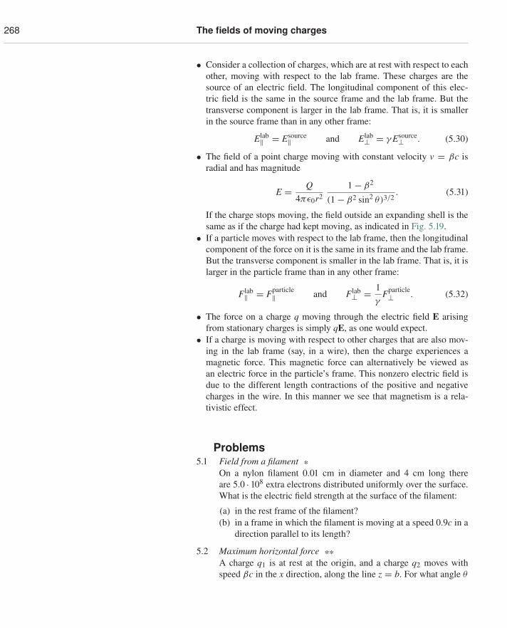
268 The fields of moving charges
• Consider a collection of charges, which are at rest with respect to eachother, moving with respect to the lab frame. These charges are thesource of an electric field. The longitudinal component of this elec-tric field is the same in the source frame and the lab frame. But thetransverse component is larger in the lab frame. That is, it is smallerin the source frame than in any other frame:
Elab‖ = Esource‖ and Elab⊥ = γ Esource⊥ . (5.30)
• The field of a point charge moving with constant velocity v = βc isradial and has magnitude
E = Q4πε0r2
1 − β2
(1 − β2 sin2 θ)3/2. (5.31)
If the charge stops moving, the field outside an expanding shell is thesame as if the charge had kept moving, as indicated in Fig. 5.19.
• If a particle moves with respect to the lab frame, then the longitudinalcomponent of the force on it is the same in its frame and the lab frame.But the transverse component is smaller in the lab frame. That is, it islarger in the particle frame than in any other frame:
Flab‖ = Fparticle‖ and Flab⊥ = 1
γFparticle⊥ . (5.32)
• The force on a charge q moving through the electric field E arisingfrom stationary charges is simply qE, as one would expect.
• If a charge is moving with respect to other charges that are also mov-ing in the lab frame (say, in a wire), then the charge experiences amagnetic force. This magnetic force can alternatively be viewed asan electric force in the particle’s frame. This nonzero electric field isdue to the different length contractions of the positive and negativecharges in the wire. In this manner we see that magnetism is a rela-tivistic effect.
Problems5.1 Field from a filament *
On a nylon filament 0.01 cm in diameter and 4 cm long thereare 5.0 · 108 extra electrons distributed uniformly over the surface.What is the electric field strength at the surface of the filament:
(a) in the rest frame of the filament?(b) in a frame in which the filament is moving at a speed 0.9c in a
direction parallel to its length?
5.2 Maximum horizontal force **A charge q1 is at rest at the origin, and a charge q2 moves withspeed βc in the x direction, along the line z = b. For what angle θ
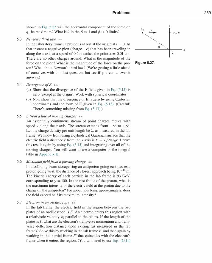
Problems 269
shown in Fig. 5.27 will the horizontal component of the force onq1 be maximum? What is θ in the β ≈ 1 and β ≈ 0 limits?
q
bc
xq1
q2
z
z = b
Figure 5.27.
5.3 Newton’s third law **In the laboratory frame, a proton is at rest at the origin at t = 0. Atthat instant a negative pion (charge −e) that has been traveling inalong the x axis at a speed of 0.6c reaches the point x = 0.01 cm.There are no other charges around. What is the magnitude of theforce on the pion? What is the magnitude of the force on the pro-ton? What about Newton’s third law? (We’re getting a little aheadof ourselves with this last question, but see if you can answer itanyway.)
5.4 Divergence of E **(a) Show that the divergence of the E field given in Eq. (5.15) is
zero (except at the origin). Work with spherical coordinates.(b) Now show that the divergence of E is zero by using Cartesian
coordinates and the form of E given in Eq. (5.13). (Careful!There’s something missing from Eq. (5.13).)
5.5 E from a line of moving charges **An essentially continuous stream of point charges moves withspeed v along the x axis. The stream extends from −∞ to +∞.Let the charge density per unit length be λ, as measured in the labframe. We know from using a cylindrical Gaussian surface that theelectric field a distance r from the x axis is E = λ/2πε0r. Derivethis result again by using Eq. (5.15) and integrating over all of themoving charges. You will want to use a computer or the integraltable in Appendix K.
5.6 Maximum field from a passing charge **In a colliding beam storage ring an antiproton going east passes aproton going west, the distance of closest approach being 10−10 m.The kinetic energy of each particle in the lab frame is 93 GeV,corresponding to γ = 100. In the rest frame of the proton, what isthe maximum intensity of the electric field at the proton due to thecharge on the antiproton? For about how long, approximately, doesthe field exceed half its maximum intensity?
5.7 Electron in an oscilloscope **In the lab frame, the electric field in the region between the twoplates of an oscilloscope is E. An electron enters this region witha relativistic velocity v0 parallel to the plates. If the length of theplates is �, what are the electron’s transverse momentum and trans-verse deflection distance upon exiting (as measured in the labframe)? Solve this by working in the lab frame F, and then again byworking in the inertial frame F′ that coincides with the electron’sframe when it enters the region. (You will need to use Eqs. (G.11)
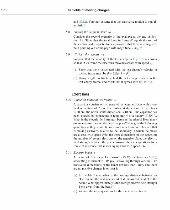
270 The fields of moving charges
and (G.12). You may assume that the transverse motion is nonrel-ativistic.)
5.8 Finding the magnetic field **Consider the second scenario in the example at the end of Sec-tion 5.8. Show that the total force in frame F′ equals the sum ofthe electric and magnetic forces, provided that there is a magneticfield pointing out of the page with magnitude γ vE2/c2.
5.9 “Twice” the velocity **Suppose that the velocity of the test charge in Fig. 5.22 is chosenso that in its frame the electrons move backward with speed v0.
(a) Show that the β associated with the test charge’s velocity inthe lab frame must be β = 2β0/(1 + β2
0 ).(b) Using length contraction, find the net charge density in the
test-charge frame, and check that it agrees with Eq. (5.24).
Exercises5.10 Capacitor plates in two frames *
A capacitor consists of two parallel rectangular plates with a ver-tical separation of 2 cm. The east–west dimension of the platesis 20 cm, the north–south dimension is 10 cm. The capacitor hasbeen charged by connecting it temporarily to a battery of 300 V.What is the electric field strength between the plates? How manyexcess electrons are on the negative plate? Now give the followingquantities as they would be measured in a frame of reference thatis moving eastward, relative to the laboratory in which the platesare at rest, with speed 0.6c: the three dimensions of the capacitor;the number of excess electrons on the negative plate; the electricfield strength between the plates. Answer the same questions for aframe of reference that is moving upward with speed 0.6c.
5.11 Electron beam *A beam of 9.5 megaelectron-volt (MeV) electrons (γ ≈ 20),amounting as current to 0.05 μA, is traveling through vacuum. Thetransverse dimensions of the beam are less than 1 mm, and thereare no positive charges in or near it.
(a) In the lab frame, what is the average distance between anelectron and the next one ahead of it, measured parallel to thebeam? What approximately is the average electric field strength1 cm away from the beam?
(b) Answer the same questions for the electron rest frame.
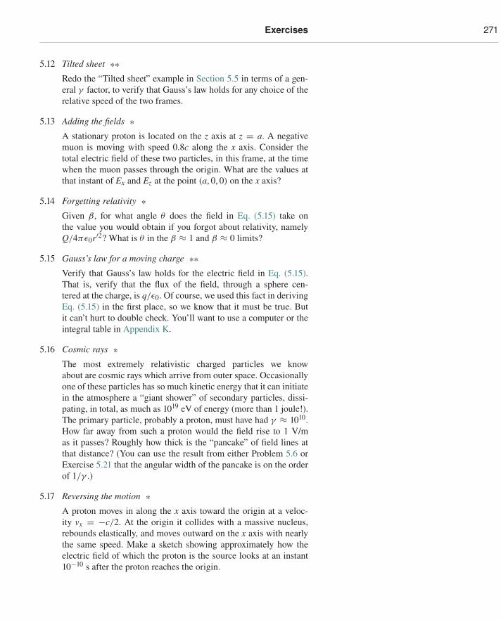
Exercises 271
5.12 Tilted sheet **Redo the “Tilted sheet” example in Section 5.5 in terms of a gen-eral γ factor, to verify that Gauss’s law holds for any choice of therelative speed of the two frames.
5.13 Adding the fields *A stationary proton is located on the z axis at z = a. A negativemuon is moving with speed 0.8c along the x axis. Consider thetotal electric field of these two particles, in this frame, at the timewhen the muon passes through the origin. What are the values atthat instant of Ex and Ez at the point (a, 0, 0) on the x axis?
5.14 Forgetting relativity *Given β, for what angle θ does the field in Eq. (5.15) take onthe value you would obtain if you forgot about relativity, namelyQ/4πε0r′2? What is θ in the β ≈ 1 and β ≈ 0 limits?
5.15 Gauss’s law for a moving charge **Verify that Gauss’s law holds for the electric field in Eq. (5.15).That is, verify that the flux of the field, through a sphere cen-tered at the charge, is q/ε0. Of course, we used this fact in derivingEq. (5.15) in the first place, so we know that it must be true. Butit can’t hurt to double check. You’ll want to use a computer or theintegral table in Appendix K.
5.16 Cosmic rays *The most extremely relativistic charged particles we knowabout are cosmic rays which arrive from outer space. Occasionallyone of these particles has so much kinetic energy that it can initiatein the atmosphere a “giant shower” of secondary particles, dissi-pating, in total, as much as 1019 eV of energy (more than 1 joule!).The primary particle, probably a proton, must have had γ ≈ 1010.How far away from such a proton would the field rise to 1 V/mas it passes? Roughly how thick is the “pancake” of field lines atthat distance? (You can use the result from either Problem 5.6 orExercise 5.21 that the angular width of the pancake is on the orderof 1/γ .)
5.17 Reversing the motion *A proton moves in along the x axis toward the origin at a veloc-ity vx = −c/2. At the origin it collides with a massive nucleus,rebounds elastically, and moves outward on the x axis with nearlythe same speed. Make a sketch showing approximately how theelectric field of which the proton is the source looks at an instant10−10 s after the proton reaches the origin.
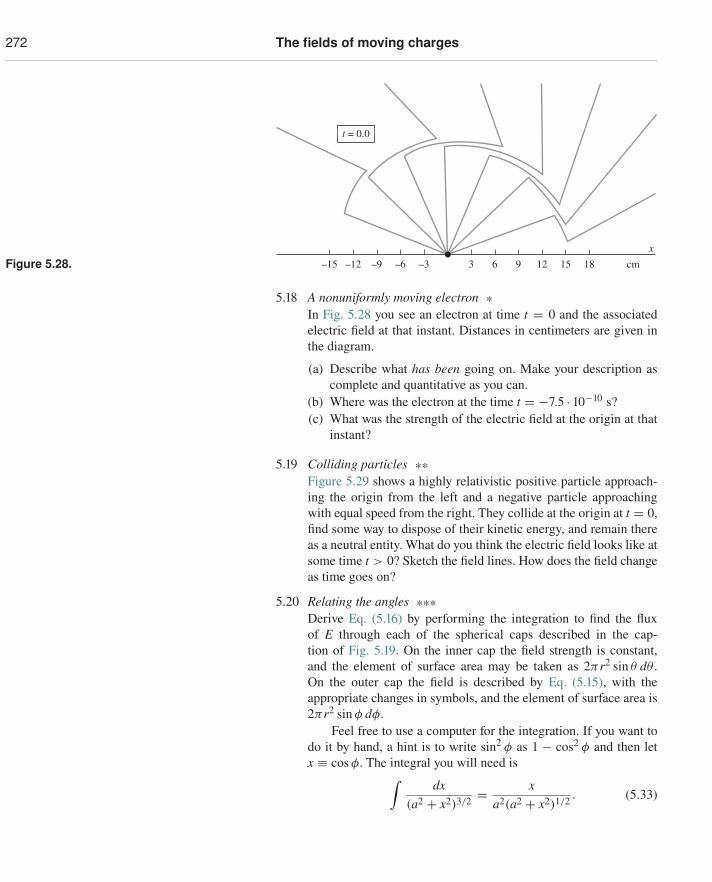
272 The fields of moving charges
Figure 5.28. –15 –12 –9 –6 –3 3 6 9 12 15 18 cm
x
t = 0.0
5.18 A nonuniformly moving electron *In Fig. 5.28 you see an electron at time t = 0 and the associatedelectric field at that instant. Distances in centimeters are given inthe diagram.
(a) Describe what has been going on. Make your description ascomplete and quantitative as you can.
(b) Where was the electron at the time t = −7.5 · 10−10 s?(c) What was the strength of the electric field at the origin at that
instant?
5.19 Colliding particles **Figure 5.29 shows a highly relativistic positive particle approach-ing the origin from the left and a negative particle approachingwith equal speed from the right. They collide at the origin at t = 0,find some way to dispose of their kinetic energy, and remain thereas a neutral entity. What do you think the electric field looks like atsome time t > 0? Sketch the field lines. How does the field changeas time goes on?
5.20 Relating the angles ***Derive Eq. (5.16) by performing the integration to find the fluxof E through each of the spherical caps described in the cap-tion of Fig. 5.19. On the inner cap the field strength is constant,and the element of surface area may be taken as 2πr2 sin θ dθ .On the outer cap the field is described by Eq. (5.15), with theappropriate changes in symbols, and the element of surface area is2πr2 sin φ dφ.
Feel free to use a computer for the integration. If you want todo it by hand, a hint is to write sin2 φ as 1 − cos2 φ and then letx ≡ cos φ. The integral you will need is∫
dx(a2 + x2)3/2 = x
a2(a2 + x2)1/2 . (5.33)
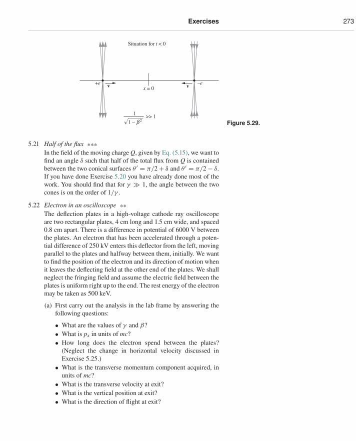
Exercises 273
+e –ev x = 0 v
Situation for t < 0
1 >> 11 − b2 Figure 5.29.
5.21 Half of the flux ***In the field of the moving charge Q, given by Eq. (5.15), we want tofind an angle δ such that half of the total flux from Q is containedbetween the two conical surfaces θ ′ = π/2 + δ and θ ′ = π/2 − δ.If you have done Exercise 5.20 you have already done most of thework. You should find that for γ � 1, the angle between the twocones is on the order of 1/γ .
5.22 Electron in an oscilloscope **The deflection plates in a high-voltage cathode ray oscilloscopeare two rectangular plates, 4 cm long and 1.5 cm wide, and spaced0.8 cm apart. There is a difference in potential of 6000 V betweenthe plates. An electron that has been accelerated through a poten-tial difference of 250 kV enters this deflector from the left, movingparallel to the plates and halfway between them, initially. We wantto find the position of the electron and its direction of motion whenit leaves the deflecting field at the other end of the plates. We shallneglect the fringing field and assume the electric field between theplates is uniform right up to the end. The rest energy of the electronmay be taken as 500 keV.
(a) First carry out the analysis in the lab frame by answering thefollowing questions:
• What are the values of γ and β?• What is px in units of mc?• How long does the electron spend between the plates?
(Neglect the change in horizontal velocity discussed inExercise 5.25.)
• What is the transverse momentum component acquired, inunits of mc?
• What is the transverse velocity at exit?• What is the vertical position at exit?• What is the direction of flight at exit?
274 The fields of moving charges
(b) Now describe this whole process as it would appear in aninertial frame that moved with the electron at the moment itentered the deflecting region. What do the plates look like?What is the field between them? What happens to the electronin this coordinate system? Your main object in this exercise isto convince yourself that the two descriptions are completelyconsistent.
5.23 Two views of an oscilloscope **In a high-voltage oscilloscope the source of electrons is a cathodeat potential −125 kV with respect to the anode and the enclosedregion beyond the anode aperture. Within this region there is apair of parallel plates 5 cm long in the x direction (the direction ofthe electron beam) and 8 mm apart in the y direction. An electronleaves the cathode with negligible velocity, is accelerated towardthe anode, and subsequently passes between the deflecting platesat a time when the potential of the lower plate is −120 V, that ofthe upper plate +120 V.
Fill in the blanks. Use rounded-off constants: electron restenergy = 5 · 105 eV, etc. When the electron arrives at the anode,its kinetic energy is eV, its total energy has increased bya factor of , and its velocity is c. Its momentumis kg m/s in the x direction. Beyond the anode the elec-tron passes between parallel metal plates. The field between theplates is V/m; the force on the electron is newtonsupward. The electron spends seconds between the platesand emerges, having acquired y momentum of magnitude py =
kg m/s. Its trajectory now slants upward at an angle θ =radians.
A fast neutron that just happened to be moving along withthe electron when it passed through the anode reported subsequentevents as follows. “We were sitting there when this capacitor cameflying at us at m/s. It was m long, so it surroundedus for seconds. That didn’t bother me, but the electric fieldof V/m accelerated the electron so that, after the capacitorleft us, the electron was moving away from me at m/s, witha momentum of kg m/s.”
5.24 Acquiring transverse momentum ***In the rest frame of a particle with charge q1, another particle withcharge q2 is approaching, moving with velocity v not small com-pared with c. If it continues to move in a straight line, it will passa distance b from the position of the first particle. It is so massivethat its displacement from the straight path during the encounteris small compared with b. Likewise, the first particle is so mas-sive that its displacement from its initial position while the otherparticle is nearby is also small compared with b.
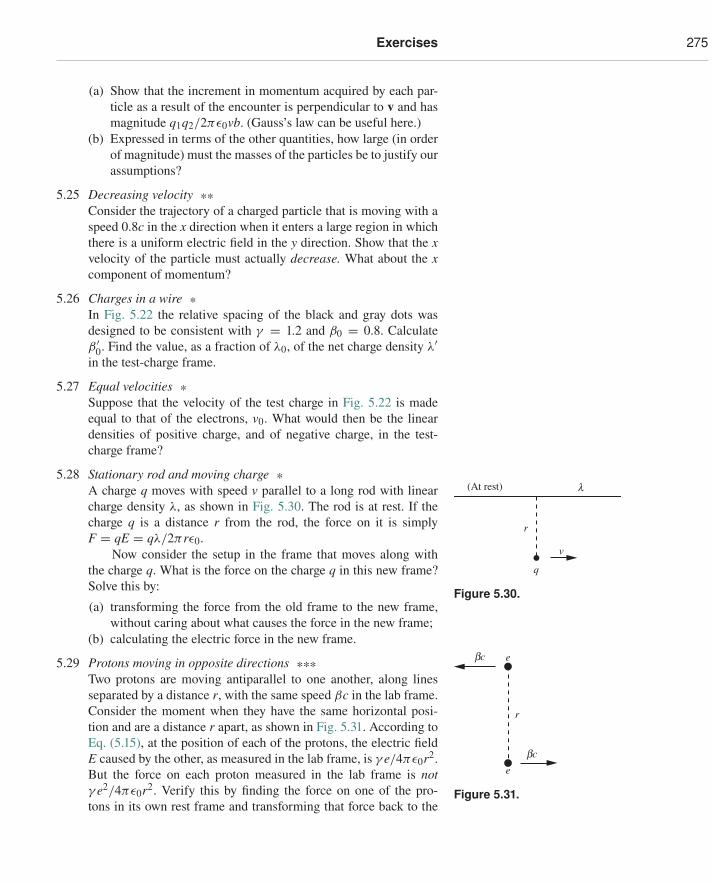
Exercises 275
(a) Show that the increment in momentum acquired by each par-ticle as a result of the encounter is perpendicular to v and hasmagnitude q1q2/2πε0vb. (Gauss’s law can be useful here.)
(b) Expressed in terms of the other quantities, how large (in orderof magnitude) must the masses of the particles be to justify ourassumptions?
5.25 Decreasing velocity **Consider the trajectory of a charged particle that is moving with aspeed 0.8c in the x direction when it enters a large region in whichthere is a uniform electric field in the y direction. Show that the xvelocity of the particle must actually decrease. What about the xcomponent of momentum?
5.26 Charges in a wire *In Fig. 5.22 the relative spacing of the black and gray dots wasdesigned to be consistent with γ = 1.2 and β0 = 0.8. Calculateβ ′
0. Find the value, as a fraction of λ0, of the net charge density λ′in the test-charge frame.
5.27 Equal velocities *Suppose that the velocity of the test charge in Fig. 5.22 is madeequal to that of the electrons, v0. What would then be the lineardensities of positive charge, and of negative charge, in the test-charge frame?
5.28 Stationary rod and moving charge *A charge q moves with speed v parallel to a long rod with linearcharge density λ, as shown in Fig. 5.30. The rod is at rest. If the
q
r
v
l(At rest)
Figure 5.30.
charge q is a distance r from the rod, the force on it is simplyF = qE = qλ/2πrε0.
Now consider the setup in the frame that moves along withthe charge q. What is the force on the charge q in this new frame?Solve this by:
(a) transforming the force from the old frame to the new frame,without caring about what causes the force in the new frame;
(b) calculating the electric force in the new frame.
5.29 Protons moving in opposite directions ***Two protons are moving antiparallel to one another, along linesseparated by a distance r, with the same speed βc in the lab frame.Consider the moment when they have the same horizontal posi-tion and are a distance r apart, as shown in Fig. 5.31. According to
bc
bc
r
e
e
Figure 5.31.
Eq. (5.15), at the position of each of the protons, the electric fieldE caused by the other, as measured in the lab frame, is γ e/4πε0r2.But the force on each proton measured in the lab frame is notγ e2/4πε0r2. Verify this by finding the force on one of the pro-tons in its own rest frame and transforming that force back to the
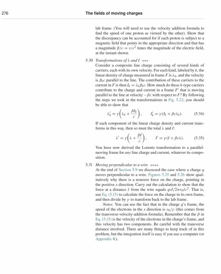
276 The fields of moving charges
lab frame. (You will need to use the velocity addition formula tofind the speed of one proton as viewed by the other). Show thatthe discrepancy can be accounted for if each proton is subject to amagnetic field that points in the appropriate direction and that hasa magnitude β/c = v/c2 times the magnitude of the electric field,at the instant shown.
5.30 Transformations of λ and I ***Consider a composite line charge consisting of several kinds ofcarriers, each with its own velocity. For each kind, labeled by k, thelinear density of charge measured in frame F is λk, and the velocityis βkc parallel to the line. The contribution of these carriers to thecurrent in F is then Ik = λkβkc. How much do these k-type carrierscontribute to the charge and current in a frame F′ that is movingparallel to the line at velocity −βc with respect to F? By followingthe steps we took in the transformations in Fig. 5.22, you shouldbe able to show that
λ′k = γ
(λk + βIk
c
), I′k = γ (Ik + βcλk). (5.34)
If each component of the linear charge density and current trans-forms in this way, then so must the total λ and I:
λ′ = γ
(λ + βI
c
), I′ = γ (I + βcλ). (5.35)
You have now derived the Lorentz transformation to a parallel-moving frame for any line charge and current, whatever its compo-sition.
5.31 Moving perpendicular to a wire ****At the end of Section 5.9 we discussed the case where a charge qmoves perpendicular to a wire. Figures 5.25 and 5.26 show qual-itatively why there is a nonzero force on the charge, pointing inthe positive x direction. Carry out the calculation to show that theforce at a distance � from the wire equals qvI/2πε0�c2. That is,use Eq. (5.15) to calculate the force on the charge in its own frame,and then divide by γ to transform back to the lab frame.
Notes: You can use the fact that in the charge q’s frame, thespeed of the electrons in the x direction is v0/γ (this comes fromthe transverse-velocity-addition formula). Remember that the β inEq. (5.15) is the velocity of the electrons in the charge’s frame, andthis velocity has two components. Be careful with the transversedistance involved. There are many things to keep track of in thisproblem, but the integration itself is easy if you use a computer (orAppendix K).
11.5 Electric currents in atoms 545
This has the dimensions of volume, just like the electric polarizabilityα/4πε0. However, it is five or six orders of magnitude smaller than typ-ical electric polarizabilities, as sampled in Table 10.2. We can be a littlemore precise about this disparity. Using Eq. (11.41), we have (recallingμ0 = 1/ε0c2)
μ0
4π
�mB1
= − r2
4μ0e2
4πme= − r2
4
(1
4πε0
e2
mec2
)≡ − r2
4r0. (11.44)
The quantity in parentheses has the dimensions of length and is knownas the classical electron radius,6 r0 = 2.8 · 10−15 m. Since the electricpolarizability is given by α/4πε0 ≈ r3, where r is an atomic radius, wesee that the magnetic polarizability is smaller than the electric polariz-ability by the ratio (roughly, up to a factor of 4 and other factors of order1 that our models ignore) of the classical electron radius r0 to an atomicradius r.
Example Let us see if Eq. (11.41) will account for the force on our diamag-netic samples listed in Table 11.1. The total number of electrons is about the samein one gram of almost anything. It is about one electron for every two nucle-ons (recall that the atomic weight is about twice the atomic number for most ofthe elements), or N = 3 · 1026 electrons per kilogram of matter. This followsfrom the fact that the mass of a nucleon is 1.67 · 10−27 kg, so there are 6 · 1026
nucleons in a kilogram. Equivalently, hydrogen has an atomic weight of 1, so thenumber of nucleons in one gram is Avogadro’s number, 6.02 · 1023.
Of course, the r2 in Eq. (11.41) must now be replaced by a mean square orbitradius 〈r2〉, where the average is taken over all the electrons in the atom, some ofwhich have larger orbits than others. Actually 〈r2〉 varies remarkably little fromatom to atom through the whole periodic table, and a2
0, the square of the Bohrradius which we have just used, remains a surprisingly good estimate. Adoptingthat, we would predict, using Eq. (11.42), that a field of 1.8 tesla would induce in1 kg of substance a magnetic moment of magnitude
�m = Ne2r2
4meB1 = (3 · 1026)(2 · 10−29 C2 m2/kg)(1.8 tesla)
= 1.1 · 10−2 jouletesla
(or amp-m2), (11.45)
which in a gradient of 17 tesla/m would give rise to a force of magnitude
F = �m∂Bz
∂z=
(1.1 · 10−2 joule
tesla
)(17
teslam
)= 0.18 newtons. (11.46)
This agrees quite well, indeed better than we had any right to expect, with thevalues for the several purely diamagnetic substances listed in Table 11.1. As far asthe sign of the force goes, we know from Eq. (11.39) that the magnetic moment is
6 This radius is obtained by setting the rest energy of the electron, mec2, equal to (inorder of magnitude) the electrostatic potential energy of a ball with radius r0 andcharge e. See Exercise 1.62.
546 Magnetic fields in matter
antiparallel to the external magnetic field. The discussion in Section 11.4 there-fore tells us that the force acts in the direction of decreasing field strength, thatis, outward from the solenoid. This agrees with the behavior of the diamagneticsamples, because the convention in Table 11.1 was that “−” meant outward.
We can see now why diamagnetism is a universal phenomenon, anda rather inconspicuous one. It is about the same in molecules as in atoms.The fact that a molecule can be a much larger structure than an atom –it may be built of hundreds or thousands of atoms – does not generallyincrease the effective mean-square orbit radius. The reason is that in amolecule any given electron is pretty well localized on an atom. Thereare some interesting exceptions, and we included one in Table 11.1 –graphite. The anomalous diamagnetism of graphite is due to an unusualstructure that permits some electrons to circulate rather freely within aplanar group of atoms in the crystal lattice. For these electrons 〈r2〉 isextraordinarily large.
As mentioned at the beginning of this section, diamagnetism (andlikewise paramagnetism and ferromagnetism) can be explained only withquantum mechanics. A purely classical theory of diamagnetism doesnot exist; see O’Dell and Zia (1986). Nevertheless, the above discus-sion is helpful for understanding the critical property of diamagnetism,namely that the change in the magnetic moment is directed opposite tothe applied magnetic field.
11.6 Electron spin and magnetic momentIn addition to its orbital angular momentum, the electron possessesanother kind of angular momentum that has nothing to do with its orbitalmotion. It behaves in many ways as if it were continually rotating aroundan axis of its own. This property is called spin. While diamagnetism isa result of the orbital angular momentum of electrons, paramagnetism isa result of their spin angular momentum (as is ferromagnetism, whichwe will discuss in Section 11.11). A consequence of these origins is thata diamagnetic moment points antiparallel to the external magnetic field,whereas a paramagnetic moment points parallel to the external field (inan average sense, as we will see).
When the magnitude of the spin angular momentum is measured,the same result is always obtained: h/4π , where h is Planck’s constant,6.626 · 10−34 kg m2/s. Electron spin is a quantum phenomenon. Its sig-nificance for us now lies in the fact that there is associated with thisintrinsic, or “built-in,” angular momentum a magnetic moment, like-wise of invariable magnitude. This magnetic moment points in the direc-tion you would expect if you visualize the electron as a ball of negativecharge spinning around its axis. That is, the magnetic moment vectorpoints antiparallel to the spin angular momentum vector, as indicated in
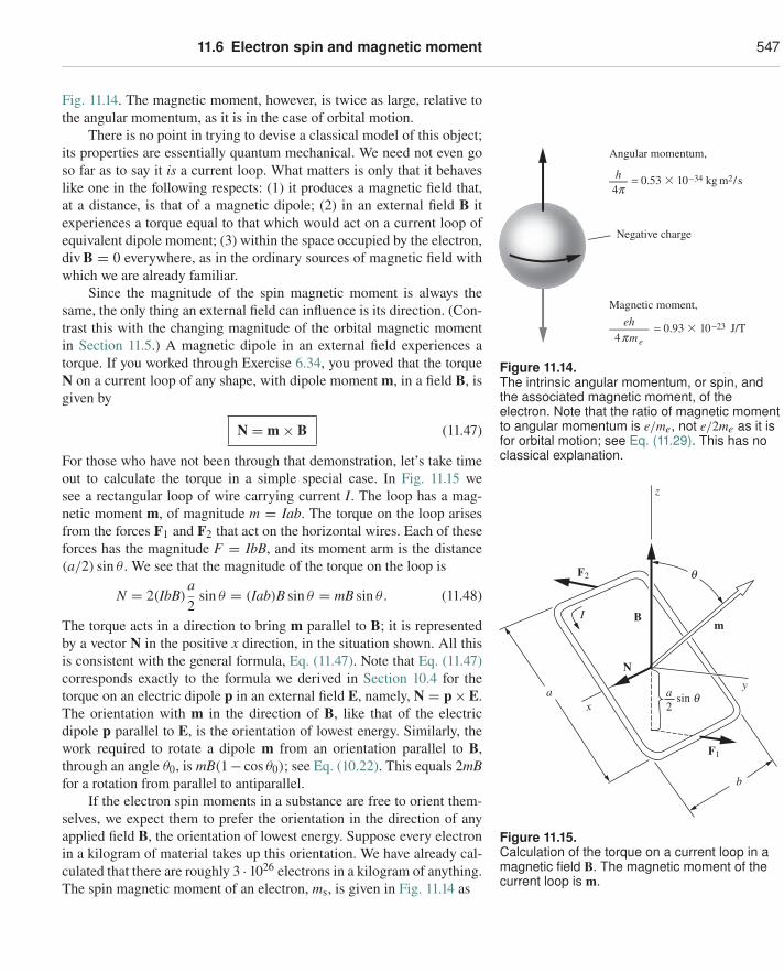
11.6 Electron spin and magnetic moment 547
Fig. 11.14. The magnetic moment, however, is twice as large, relative tothe angular momentum, as it is in the case of orbital motion.
There is no point in trying to devise a classical model of this object;its properties are essentially quantum mechanical. We need not even goso far as to say it is a current loop. What matters is only that it behaveslike one in the following respects: (1) it produces a magnetic field that,at a distance, is that of a magnetic dipole; (2) in an external field B itexperiences a torque equal to that which would act on a current loop ofequivalent dipole moment; (3) within the space occupied by the electron,div B = 0 everywhere, as in the ordinary sources of magnetic field withwhich we are already familiar.
Angular momentum,
Negative charge
Magnetic moment,
= 0.53 � 10−34 kg m2/sh4p
= 0.93 � 10−23 J/T4pme
eh
Figure 11.14.The intrinsic angular momentum, or spin, andthe associated magnetic moment, of theelectron. Note that the ratio of magnetic momentto angular momentum is e/me, not e/2me as it isfor orbital motion; see Eq. (11.29). This has noclassical explanation.
Since the magnitude of the spin magnetic moment is always thesame, the only thing an external field can influence is its direction. (Con-trast this with the changing magnitude of the orbital magnetic momentin Section 11.5.) A magnetic dipole in an external field experiences atorque. If you worked through Exercise 6.34, you proved that the torqueN on a current loop of any shape, with dipole moment m, in a field B, isgiven by
N = m × B (11.47)
For those who have not been through that demonstration, let’s take time
F2
F1
I B
N
m
z
y
b
2a a
xsin q
q
Figure 11.15.Calculation of the torque on a current loop in amagnetic field B. The magnetic moment of thecurrent loop is m.
out to calculate the torque in a simple special case. In Fig. 11.15 wesee a rectangular loop of wire carrying current I. The loop has a mag-netic moment m, of magnitude m = Iab. The torque on the loop arisesfrom the forces F1 and F2 that act on the horizontal wires. Each of theseforces has the magnitude F = IbB, and its moment arm is the distance(a/2) sin θ . We see that the magnitude of the torque on the loop is
N = 2(IbB)a2
sin θ = (Iab)B sin θ = mB sin θ . (11.48)
The torque acts in a direction to bring m parallel to B; it is representedby a vector N in the positive x direction, in the situation shown. All thisis consistent with the general formula, Eq. (11.47). Note that Eq. (11.47)corresponds exactly to the formula we derived in Section 10.4 for thetorque on an electric dipole p in an external field E, namely, N = p×E.The orientation with m in the direction of B, like that of the electricdipole p parallel to E, is the orientation of lowest energy. Similarly, thework required to rotate a dipole m from an orientation parallel to B,through an angle θ0, is mB(1− cos θ0); see Eq. (10.22). This equals 2mBfor a rotation from parallel to antiparallel.
If the electron spin moments in a substance are free to orient them-selves, we expect them to prefer the orientation in the direction of anyapplied field B, the orientation of lowest energy. Suppose every electronin a kilogram of material takes up this orientation. We have already cal-culated that there are roughly 3 · 1026 electrons in a kilogram of anything.The spin magnetic moment of an electron, ms, is given in Fig. 11.14 as
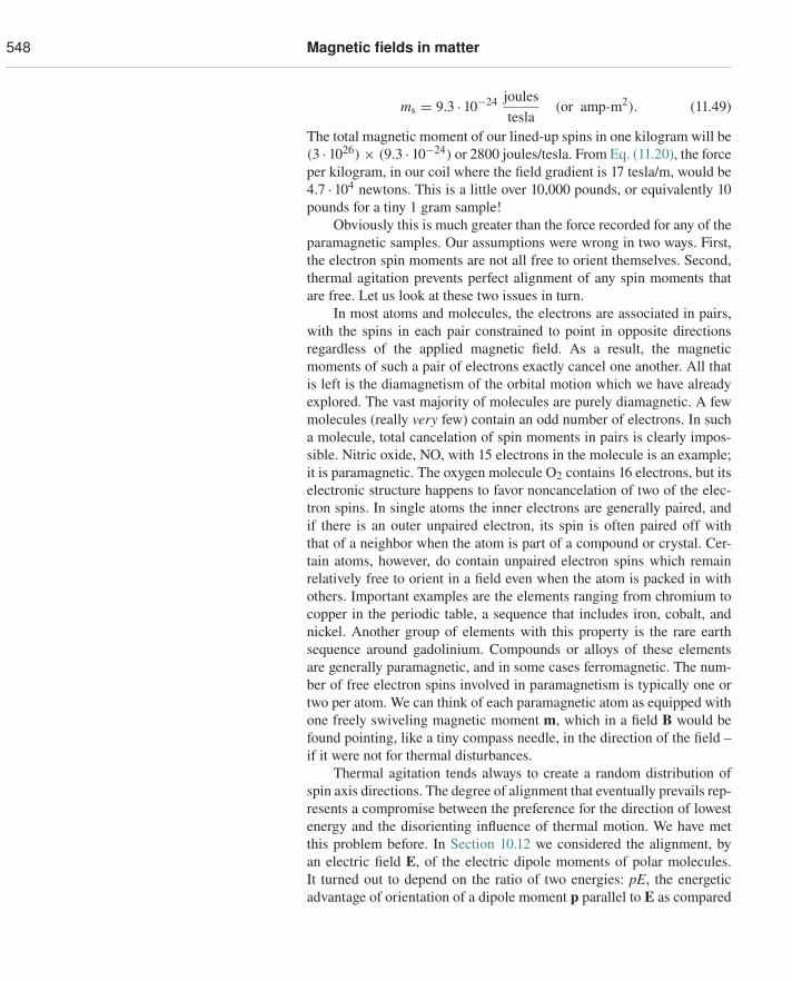
548 Magnetic fields in matter
ms = 9.3 · 10−24 joulestesla
(or amp-m2). (11.49)
The total magnetic moment of our lined-up spins in one kilogram will be(3 · 1026) × (9.3 · 10−24) or 2800 joules/tesla. From Eq. (11.20), the forceper kilogram, in our coil where the field gradient is 17 tesla/m, would be4.7 · 104 newtons. This is a little over 10,000 pounds, or equivalently 10pounds for a tiny 1 gram sample!
Obviously this is much greater than the force recorded for any of theparamagnetic samples. Our assumptions were wrong in two ways. First,the electron spin moments are not all free to orient themselves. Second,thermal agitation prevents perfect alignment of any spin moments thatare free. Let us look at these two issues in turn.
In most atoms and molecules, the electrons are associated in pairs,with the spins in each pair constrained to point in opposite directionsregardless of the applied magnetic field. As a result, the magneticmoments of such a pair of electrons exactly cancel one another. All thatis left is the diamagnetism of the orbital motion which we have alreadyexplored. The vast majority of molecules are purely diamagnetic. A fewmolecules (really very few) contain an odd number of electrons. In sucha molecule, total cancelation of spin moments in pairs is clearly impos-sible. Nitric oxide, NO, with 15 electrons in the molecule is an example;it is paramagnetic. The oxygen molecule O2 contains 16 electrons, but itselectronic structure happens to favor noncancelation of two of the elec-tron spins. In single atoms the inner electrons are generally paired, andif there is an outer unpaired electron, its spin is often paired off withthat of a neighbor when the atom is part of a compound or crystal. Cer-tain atoms, however, do contain unpaired electron spins which remainrelatively free to orient in a field even when the atom is packed in withothers. Important examples are the elements ranging from chromium tocopper in the periodic table, a sequence that includes iron, cobalt, andnickel. Another group of elements with this property is the rare earthsequence around gadolinium. Compounds or alloys of these elementsare generally paramagnetic, and in some cases ferromagnetic. The num-ber of free electron spins involved in paramagnetism is typically one ortwo per atom. We can think of each paramagnetic atom as equipped withone freely swiveling magnetic moment m, which in a field B would befound pointing, like a tiny compass needle, in the direction of the field –if it were not for thermal disturbances.
Thermal agitation tends always to create a random distribution ofspin axis directions. The degree of alignment that eventually prevails rep-resents a compromise between the preference for the direction of lowestenergy and the disorienting influence of thermal motion. We have metthis problem before. In Section 10.12 we considered the alignment, byan electric field E, of the electric dipole moments of polar molecules.It turned out to depend on the ratio of two energies: pE, the energeticadvantage of orientation of a dipole moment p parallel to E as compared
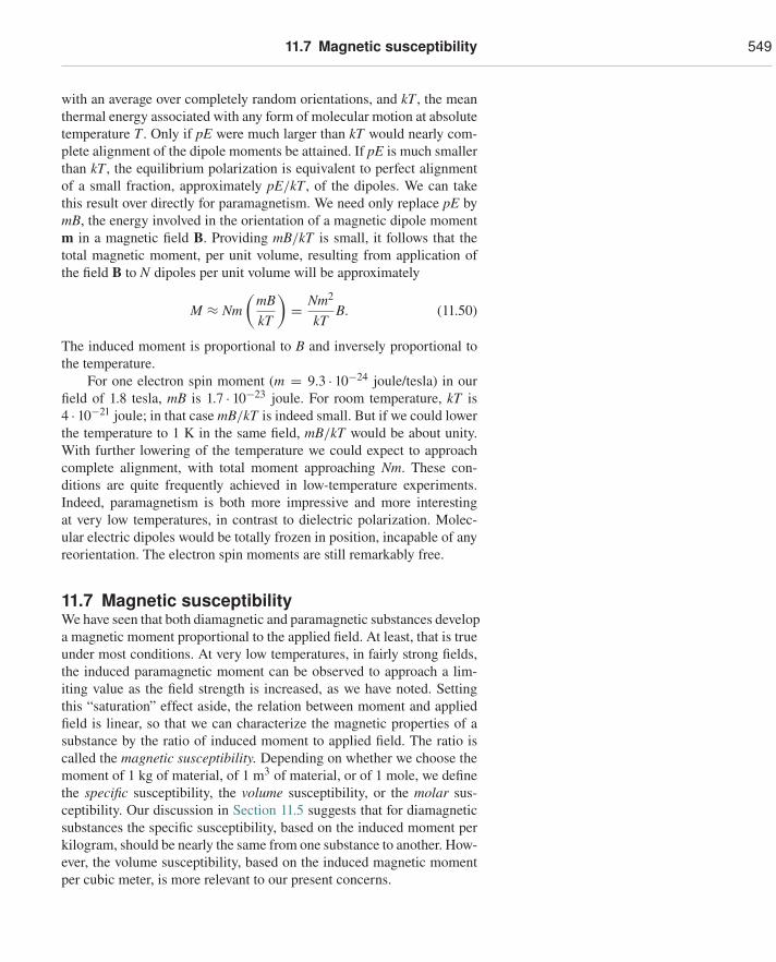
11.7 Magnetic susceptibility 549
with an average over completely random orientations, and kT , the meanthermal energy associated with any form of molecular motion at absolutetemperature T . Only if pE were much larger than kT would nearly com-plete alignment of the dipole moments be attained. If pE is much smallerthan kT , the equilibrium polarization is equivalent to perfect alignmentof a small fraction, approximately pE/kT , of the dipoles. We can takethis result over directly for paramagnetism. We need only replace pE bymB, the energy involved in the orientation of a magnetic dipole momentm in a magnetic field B. Providing mB/kT is small, it follows that thetotal magnetic moment, per unit volume, resulting from application ofthe field B to N dipoles per unit volume will be approximately
M ≈ Nm(
mBkT
)= Nm2
kTB. (11.50)
The induced moment is proportional to B and inversely proportional tothe temperature.
For one electron spin moment (m = 9.3 · 10−24 joule/tesla) in ourfield of 1.8 tesla, mB is 1.7 · 10−23 joule. For room temperature, kT is4 · 10−21 joule; in that case mB/kT is indeed small. But if we could lowerthe temperature to 1 K in the same field, mB/kT would be about unity.With further lowering of the temperature we could expect to approachcomplete alignment, with total moment approaching Nm. These con-ditions are quite frequently achieved in low-temperature experiments.Indeed, paramagnetism is both more impressive and more interestingat very low temperatures, in contrast to dielectric polarization. Molec-ular electric dipoles would be totally frozen in position, incapable of anyreorientation. The electron spin moments are still remarkably free.
11.7 Magnetic susceptibilityWe have seen that both diamagnetic and paramagnetic substances developa magnetic moment proportional to the applied field. At least, that is trueunder most conditions. At very low temperatures, in fairly strong fields,the induced paramagnetic moment can be observed to approach a lim-iting value as the field strength is increased, as we have noted. Settingthis “saturation” effect aside, the relation between moment and appliedfield is linear, so that we can characterize the magnetic properties of asubstance by the ratio of induced moment to applied field. The ratio iscalled the magnetic susceptibility. Depending on whether we choose themoment of 1 kg of material, of 1 m3 of material, or of 1 mole, we definethe specific susceptibility, the volume susceptibility, or the molar sus-ceptibility. Our discussion in Section 11.5 suggests that for diamagneticsubstances the specific susceptibility, based on the induced moment perkilogram, should be nearly the same from one substance to another. How-ever, the volume susceptibility, based on the induced magnetic momentper cubic meter, is more relevant to our present concerns.
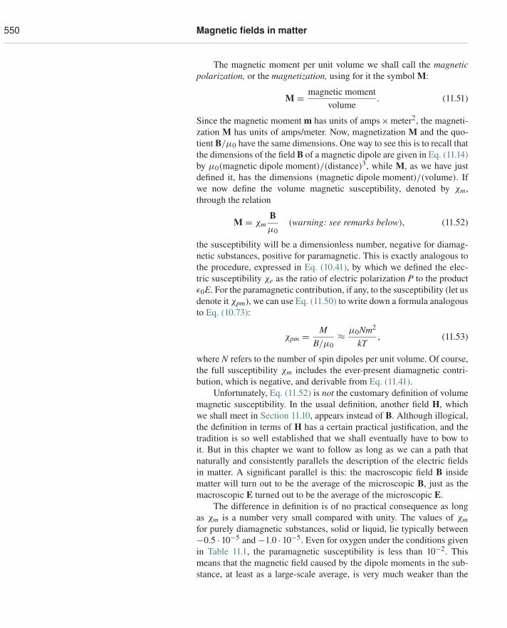
550 Magnetic fields in matter
The magnetic moment per unit volume we shall call the magneticpolarization, or the magnetization, using for it the symbol M:
M = magnetic momentvolume
. (11.51)
Since the magnetic moment m has units of amps×meter2, the magneti-zation M has units of amps/meter. Now, magnetization M and the quo-tient B/μ0 have the same dimensions. One way to see this is to recall thatthe dimensions of the field B of a magnetic dipole are given in Eq. (11.14)by μ0(magnetic dipole moment)/(distance)3, while M, as we have justdefined it, has the dimensions (magnetic dipole moment)/(volume). Ifwe now define the volume magnetic susceptibility, denoted by χm,through the relation
M = χmBμ0
(warning: see remarks below), (11.52)
the susceptibility will be a dimensionless number, negative for diamag-netic substances, positive for paramagnetic. This is exactly analogous tothe procedure, expressed in Eq. (10.41), by which we defined the elec-tric susceptibility χe as the ratio of electric polarization P to the productε0E. For the paramagnetic contribution, if any, to the susceptibility (let usdenote it χpm), we can use Eq. (11.50) to write down a formula analogousto Eq. (10.73):
χpm = MB/μ0
≈ μ0Nm2
kT, (11.53)
where N refers to the number of spin dipoles per unit volume. Of course,the full susceptibility χm includes the ever-present diamagnetic contri-bution, which is negative, and derivable from Eq. (11.41).
Unfortunately, Eq. (11.52) is not the customary definition of volumemagnetic susceptibility. In the usual definition, another field H, whichwe shall meet in Section 11.10, appears instead of B. Although illogical,the definition in terms of H has a certain practical justification, and thetradition is so well established that we shall eventually have to bow toit. But in this chapter we want to follow as long as we can a path thatnaturally and consistently parallels the description of the electric fieldsin matter. A significant parallel is this: the macroscopic field B insidematter will turn out to be the average of the microscopic B, just as themacroscopic E turned out to be the average of the microscopic E.
The difference in definition is of no practical consequence as longas χm is a number very small compared with unity. The values of χmfor purely diamagnetic substances, solid or liquid, lie typically between−0.5 · 10−5 and −1.0 · 10−5. Even for oxygen under the conditions givenin Table 11.1, the paramagnetic susceptibility is less than 10−2. Thismeans that the magnetic field caused by the dipole moments in the sub-stance, at least as a large-scale average, is very much weaker than the
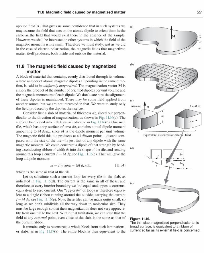
11.8 Magnetic field caused by magnetized matter 551
applied field B. That gives us some confidence that in such systems wemay assume the field that acts on the atomic dipole to orient them is thesame as the field that would exist there in the absence of the sample.However, we shall be interested in other systems in which the field of themagnetic moments is not small. Therefore we must study, just as we didin the case of electric polarization, the magnetic fields that magnetizedmatter itself produces, both inside and outside the material.
11.8 The magnetic field caused by magnetizedmatter
A block of material that contains, evenly distributed through its volume,a large number of atomic magnetic dipoles all pointing in the same direc-tion, is said to be uniformly magnetized. The magnetization vector M issimply the product of the number of oriented dipoles per unit volume andthe magnetic moment m of each dipole. We don’t care how the alignmentof these dipoles is maintained. There may be some field applied fromanother source, but we are not interested in that. We want to study onlythe field produced by the dipoles themselves.
M
mArea da
(a)
(b)
(c)
(d)
(e)
dz
I = M dz
I
I
I
I
I
I
dz
Equivalent, as sources of external field
Figure 11.16.The thin slab, magnetized perpendicular to itsbroad surface, is equivalent to a ribbon ofcurrent so far as its external field is concerned.
Consider first a slab of material of thickness dz, sliced out perpen-dicular to the direction of magnetization, as shown in Fig. 11.16(a). Theslab can be divided into little tiles, as indicated in Fig. 11.16(b). One suchtile, which has a top surface of area da, contains a total dipole momentamounting to M da dz, since M is the dipole moment per unit volume.The magnetic field this tile produces at all distant points – distant com-pared with the size of the tile – is just that of any dipole with the samemagnetic moment. We could construct a dipole of that strength by bend-ing a conducting ribbon of width dz into the shape of the tile, and sendingaround this loop a current I = M dz; see Fig. 11.16(c). That will give theloop a dipole moment:
m = I × area = (M dz) da, (11.54)
which is the same as that of the tile.Let us substitute such a current loop for every tile in the slab, as
indicated in Fig. 11.16(d). The current is the same in all of these, andtherefore, at every interior boundary we find equal and opposite currents,equivalent to zero current. Our “egg-crate” of loops is therefore equiva-lent to a single ribbon running around the outside, carrying the currentI =M dz; see Fig. 11.16(e). Now, these tiles can be made quite small, solong as we don’t subdivide all the way down to molecular size. Theymust be large enough so that their magnetization does not vary apprecia-bly from one tile to the next. Within that limitation, we can state that thefield at any external point, even close to the slab, is the same as that ofthe current ribbon.
It remains only to reconstruct a whole block from such laminations,or slabs, as in Fig. 11.17(a). The entire block is then equivalent to the
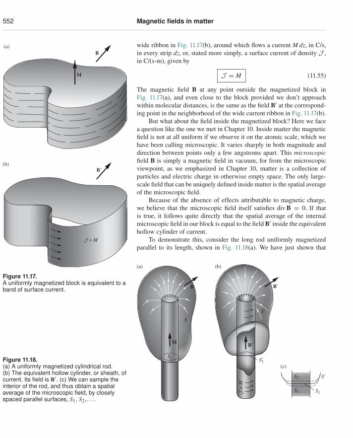
552 Magnetic fields in matter
wide ribbon in Fig. 11.17(b), around which flows a current M dz, in C/s,in every strip dz, or, stated more simply, a surface current of density J ,in C/(s-m), given by
J = M (11.55)
The magnetic field B at any point outside the magnetized block inFig. 11.17(a), and even close to the block provided we don’t approachwithin molecular distances, is the same as the field B′ at the correspond-ing point in the neighborhood of the wide current ribbon in Fig. 11.17(b).
But what about the field inside the magnetized block? Here we facea question like the one we met in Chapter 10. Inside matter the magneticfield is not at all uniform if we observe it on the atomic scale, which wehave been calling microscopic. It varies sharply in both magnitude anddirection between points only a few angstroms apart. This microscopicfield B is simply a magnetic field in vacuum, for from the microscopicviewpoint, as we emphasized in Chapter 10, matter is a collection ofparticles and electric charge in otherwise empty space. The only large-scale field that can be uniquely defined inside matter is the spatial averageof the microscopic field.
(b)
(a)
M
B
B�
= M
Figure 11.17.A uniformly magnetized block is equivalent to aband of surface current.
Because of the absence of effects attributable to magnetic charge,we believe that the microscopic field itself satisfies div B = 0. If thatis true, it follows quite directly that the spatial average of the internalmicroscopic field in our block is equal to the field B′ inside the equivalenthollow cylinder of current.
To demonstrate this, consider the long rod uniformly magnetizedparallel to its length, shown in Fig. 11.18(a). We have just shown that
Figure 11.18.(a) A uniformly magnetized cylindrical rod.(b) The equivalent hollow cylinder, or sheath, ofcurrent. Its field is B′. (c) We can sample theinterior of the rod, and thus obtain a spatialaverage of the microscopic field, by closelyspaced parallel surfaces, S1, S2,. . . .
B
S
(a)
S�
B�
S�
S1
S2
S3 S1
S�1
(b)
(c)
M
B�
= M
11.8 Magnetic field caused by magnetized matter 553
the external field will be the same as that of the long cylinder of current(practically equivalent to a single-layer solenoid) shown in Fig. 11.18(b).The surface S in Fig. 11.18(a) indicates a closed surface that includes aportion S1 passing through the interior of the rod. Because div B = 0for the internal microscopic field, as well as for the external field, div Bis zero throughout the entire volume enclosed by S. It then follows fromGauss’s theorem that the surface integral of B over S must be zero. Thesurface integral of B′ over the closed surface S′ in Fig. 11.18(b) is zeroalso. Over the portions of S and S′ external to the cylinders, B and B′are identical. Therefore the surface integral of B over the internal diskS1 must be equal to the surface integral of B′ over the internal disk S′1.This must hold also for any one of a closely spaced set of parallel disks,such as S2, S3, etc., indicated in Fig. 11.18(c), because the field outside thecylinder in this neighborhood is negligibly small, so that the outside partsdon’t change anything. Now, taking the surface integral over a series ofequally spaced planes like this is a perfectly good way to compute thevolume average of the field B in that neighborhood, for it samples allvolume elements impartially. It follows that the spatial average of themicroscopic field B inside the magnetized rod is equal to the field B′inside the current sheath of Fig. 11.18(b).
It is instructive to compare the arguments we have just developedwith our analysis of the corresponding questions in Chapter 10.Figure 11.19 displays these developments side by side. You will see thatthey run logically parallel, but that at each stage there is a differencethat reflects the essential asymmetry epitomized in the observation thatelectric charges are the source of electric fields, while moving electriccharges are the source of magnetic fields. For example, in the argumentsabout the average of the microscopic field, the key to the problem in theelectric case is the assumption that curl E = 0 for the microscopic elec-tric field. In the magnetic case, the key is the assumption that div B = 0for the microscopic magnetic field.
If the magnetization M within a volume of material is not uniformbut instead varies with position as M(x, y, z), the equivalent current dis-tribution is given simply by
J = curl M (11.56)
Let’s see how this comes about in one situation. Suppose there is a mag-netization in the z direction that gets stronger as we proceed in the y direc-tion. This is represented in Fig. 11.20(a), which shows a small region inthe material subdivided into little blocks. The blocks are supposed to beso small that we may consider the magnetization uniform within a singleblock. Then we can replace each block by a current ribbon, with surfacecurrent density J = Mz. The current I carried by such a ribbon, if theblock is �z in height, is J�z or Mz�z. Now, each ribbon has a bit more
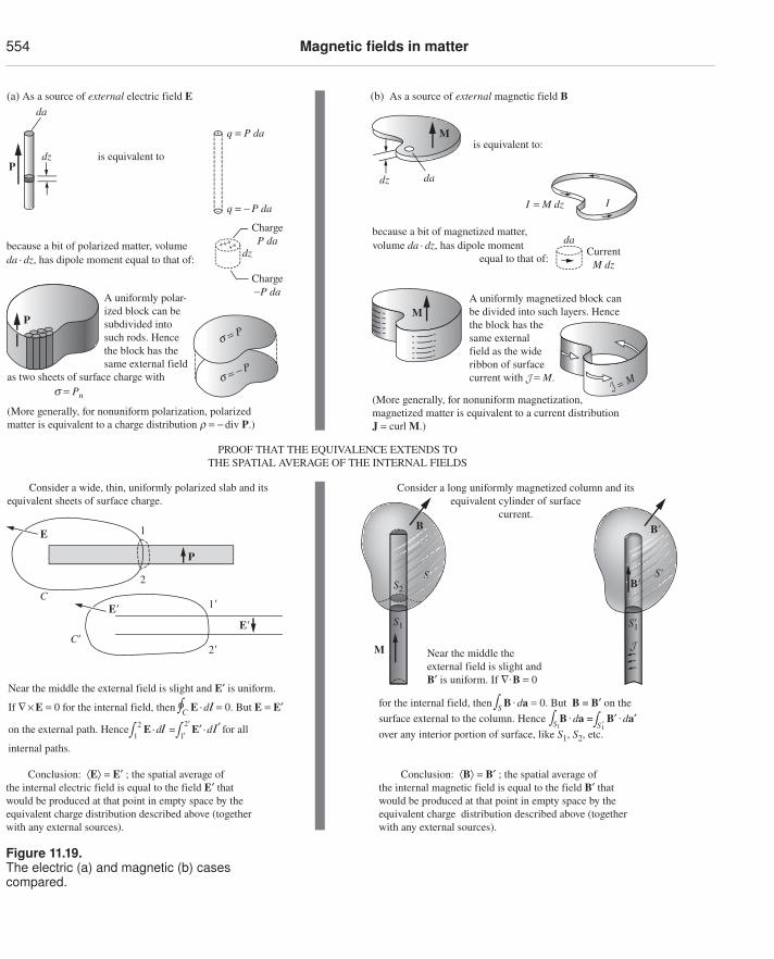
554 Magnetic fields in matter
1
2
1�
M2�
P
E
E�
E�
C
C�
S
B�
S1
B
dz
da
P
M
dadz
dz
ChargeP da
Charge−P da
s = Pn
I
M
(a) As a source of external electric field E (b) As a source of external magnetic field B
is equivalent to:
(More generally, for nonuniform magnetization,magnetized matter is equivalent to a current distributionJ = curl M.)
A uniformly magnetized block canbe divided into such layers. Hencethe block has thesame externalfield as the wideribbon of surfacecurrent with = M.
because a bit of magnetized matter,volume da · dz, has dipole moment equal to that of:
is equivalent to
because a bit of polarized matter, volumeda · dz, has dipole moment equal to that of:
q = P da+
− q = − P da
A uniformly polar-ized block can besubdivided intosuch rods. Hencethe block has thesame external field
as two sheets of surface charge with
Consider a wide, thin, uniformly polarized slab and itsequivalent sheets of surface charge.
(More generally, for nonuniform polarization, polarizedmatter is equivalent to a charge distribution r = − div P.)
PROOF THAT THE EQUIVALENCE EXTENDS TOTHE SPATIAL AVERAGE OF THE INTERNAL FIELDS
Consider a long uniformly magnetized column and itsequivalent cylinder of surface
current.
Conclusion: ⟨B⟩ = B′ ; the spatial average ofthe internal magnetic field is equal to the field B′ thatwould be produced at that point in empty space by theequivalent charge distribution described above (togetherwith any external sources).
Conclusion: ⟨E⟩ = E′ ; the spatial average ofthe internal electric field is equal to the field E′ thatwould be produced at that point in empty space by theequivalent charge distribution described above (togetherwith any external sources).
daCurrent
M dz
I = M dz
S�1
for the internal field, then B . da = 0. But B = B′ on the surface external to the column. Hence B . da = B′ . da′over any interior portion of surface, like S1, S2, etc.
Ú SÚ S1 Ú S1
+++++
P
s = P
s = − P
on the external path. Hence E ·d = E′ ·d for all
internal paths.Ú 1
2 Ú 1′2′ ′
Near the middle the external field is slight and E′ is uniform.
If ∇ × E = 0 for the internal field, then E ·d = 0. But E = E′Ú οC
Near the middle theexternal field is slight andB′ is uniform. If ∇.B = 0
SSSS2
S'B�
′
Figure 11.19.The electric (a) and magnetic (b) casescompared.
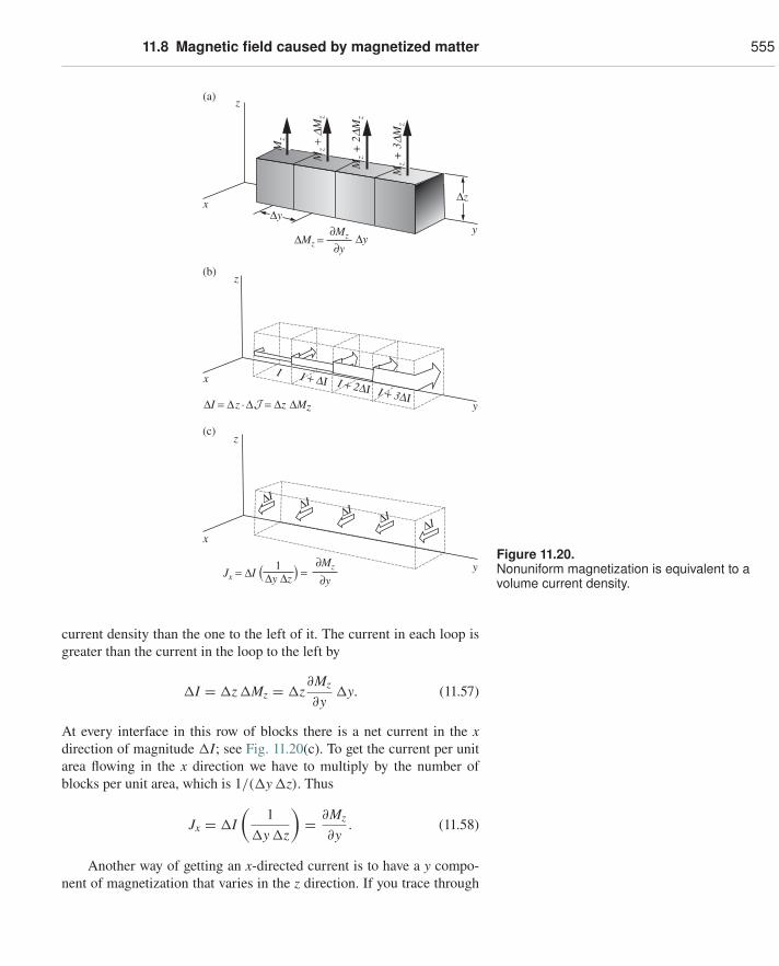
11.8 Magnetic field caused by magnetized matter 555
z
z
x
x
y
y
x
z
y
Δy
Δz
ΔI = Δz · Δ = Δz ΔMz
ΔI ΔI
ΔI ΔI
ΔI
(b)
(a)
(c)
Mz +
DM
z
Mz +
2DM
z
Mz +
3DM
z
Mz
I I + ΔI I + 2ΔI I + 3ΔI
∂Mz
Δy Δz1
∂y( )Jx = ΔI =
∂Mz
∂yΔMz Δy=
Figure 11.20.Nonuniform magnetization is equivalent to avolume current density.
current density than the one to the left of it. The current in each loop isgreater than the current in the loop to the left by
�I = �z �Mz = �z∂Mz
∂y�y. (11.57)
At every interface in this row of blocks there is a net current in the xdirection of magnitude �I; see Fig. 11.20(c). To get the current per unitarea flowing in the x direction we have to multiply by the number ofblocks per unit area, which is 1/(�y �z). Thus
Jx = �I(
1�y �z
)= ∂Mz
∂y. (11.58)
Another way of getting an x-directed current is to have a y compo-nent of magnetization that varies in the z direction. If you trace through
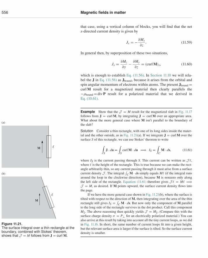
556 Magnetic fields in matter
that case, using a vertical column of blocks, you will find that the netx-directed current density is given by
Jx = −∂My
∂z. (11.59)
In general then, by superposition of these two situations,
Jx = ∂Mz
∂y− ∂My
∂z= (curl M)x, (11.60)
which is enough to establish Eq. (11.56). In Section 11.10 we will rela-bel the J in Eq. (11.56) as Jbound, because it arises from the orbital andspin angular momentum of electrons within atoms. The present Jbound =curl M result for a magnetized material then clearly parallels the−ρbound = div P result for a polarized material that we derived inEq. (10.61).
Example Show that the J = M result for the magnetized slab in Fig. 11.17follows from J = curl M, by integrating J = curl M over an appropriate area.What about the more general case where M isn’t parallel to the boundary ofthe slab?
M
M
(a)
(b)
Figure 11.21.The surface integral over a thin rectangle at theboundary, combined with Stokes’ theorem,shows that J = M follows from J = curl M.
Solution Consider a thin rectangle, with one of its long sides inside the mater-ial and the other outside, as in Fig. 11.21(a). If we integrate J = curl M over thesurface S of this rectangle, we can use Stokes’ theorem to write
∫S
J · da =∫
Scurl M · da �⇒ IS =
∫C
M · ds, (11.61)
where IS is the current passing through S. This current can be written as J �,where � is the height of the rectangle. This is true because we can make the rect-angle arbitrarily thin, so any current passing through it must arise from a surfacecurrent density J . The integral
∫C M · ds simply equals M� (if the integral runs
around the loop in the clockwise direction), because M is nonzero only alongthe left side of the rectangle. Equation (11.61) therefore gives J � = M� �⇒J = M, as desired. If M points upward, the surface current density flows intothe page.
If we have the more general case shown in Fig. 11.21(b), where the surface istilted with respect to the direction of M, then integrating over the area of the thinrectangle still gives IS = ∫
C M · ds. But now only the component of M parallelto the long side of the rectangle survives in the dot product. Call this componentM‖. The above reasoning then quickly yields J = M‖. (Compare this with thesurface charge density σ = P⊥ for an electrically polarized material.) You canalso arrive at this result by taking into account all the tiny current loops, as we didin Fig. 11.16. In short, the same number of current loops fit into a given height,but the relevant surface area is larger if the surface is tilted. So the surface currentdensity is smaller.
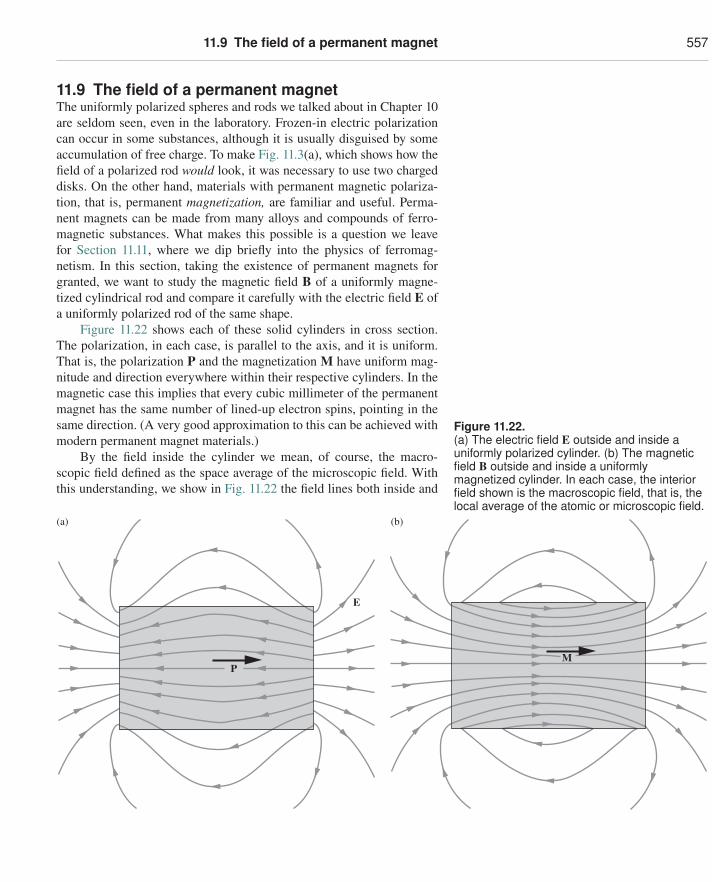
11.9 The field of a permanent magnet 557
11.9 The field of a permanent magnetThe uniformly polarized spheres and rods we talked about in Chapter 10are seldom seen, even in the laboratory. Frozen-in electric polarizationcan occur in some substances, although it is usually disguised by someaccumulation of free charge. To make Fig. 11.3(a), which shows how thefield of a polarized rod would look, it was necessary to use two chargeddisks. On the other hand, materials with permanent magnetic polariza-tion, that is, permanent magnetization, are familiar and useful. Perma-nent magnets can be made from many alloys and compounds of ferro-magnetic substances. What makes this possible is a question we leavefor Section 11.11, where we dip briefly into the physics of ferromag-netism. In this section, taking the existence of permanent magnets forgranted, we want to study the magnetic field B of a uniformly magne-tized cylindrical rod and compare it carefully with the electric field E ofa uniformly polarized rod of the same shape.
Figure 11.22 shows each of these solid cylinders in cross section.The polarization, in each case, is parallel to the axis, and it is uniform.That is, the polarization P and the magnetization M have uniform mag-nitude and direction everywhere within their respective cylinders. In themagnetic case this implies that every cubic millimeter of the permanentmagnet has the same number of lined-up electron spins, pointing in thesame direction. (A very good approximation to this can be achieved withmodern permanent magnet materials.)
By the field inside the cylinder we mean, of course, the macro-scopic field defined as the space average of the microscopic field. Withthis understanding, we show in Fig. 11.22 the field lines both inside and
Figure 11.22.(a) The electric field E outside and inside auniformly polarized cylinder. (b) The magneticfield B outside and inside a uniformlymagnetized cylinder. In each case, the interiorfield shown is the macroscopic field, that is, thelocal average of the atomic or microscopic field.
(a) (b)
E
PM
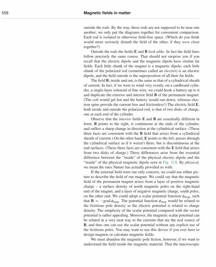
558 Magnetic fields in matter
outside the rods. By the way, these rods are not supposed to be near oneanother; we only put the diagrams together for convenient comparison.Each rod is isolated in otherwise field-free space. (Which do you thinkwould more seriously disturb the field of the other, if they were closetogether?)
Outside the rods the fields E and B look alike. In fact the field linesfollow precisely the same course. That should not surprise you if yourecall that the electric dipole and the magnetic dipole have similar farfields. Each little chunk of the magnet is a magnetic dipole, each littlechunk of the polarized rod (sometimes called an electret) is an electricdipole, and the field outside is the superposition of all their far fields.
The field B, inside and out, is the same as that of a cylindrical sheathof current. In fact, if we were to wind very evenly, on a cardboard cylin-der, a single-layer solenoid of fine wire, we could hook a battery up to itand duplicate the exterior and interior field B of the permanent magnet.(The coil would get hot and the battery would run down, whereas elec-tron spins provide the current free and frictionless!) The electric field E,both inside and outside the polarized rod, is that of two disks of charge,one at each end of the cylinder.
Observe that the interior fields E and B are essentially different inform: B points to the right, is continuous at the ends of the cylinder,and suffers a sharp change in direction at the cylindrical surface. (Thesethree facts are consistent with the B field that arises from a cylindricalsheath of current.) On the other hand, E points to the left, passes throughthe cylindrical surface as if it weren’t there, but is discontinuous at theend surfaces. (These three facts are consistent with the E field that arisesfrom two disks of charge.) These differences arise from the essentialdifference between the “inside” of the physical electric dipole and the“inside” of the physical magnetic dipole seen in Fig. 11.8. By physical,we mean the ones Nature has actually provided us with.
If the external field were our only concern, we could use either pic-ture to describe the field of our magnet. We could say that the magneticfield of the permanent magnet arises from a layer of positive magneticcharge – a surface density of north magnetic poles on the right-handend of the magnet, and a layer of negative magnetic charge, south poles,on the other end. We could adopt a scalar potential function φmag, suchthat B = −grad φmag. The potential function φmag would be related tothe fictitious pole density as the electric potential is related to chargedensity. The simplicity of the scalar potential compared with the vectorpotential is rather appealing. Moreover, the magnetic scalar potential canbe related in a very neat way to the currents that are the real source ofB, and thus one can use the scalar potential without any explicit use ofthe fictitious poles. You may want to use this device if you ever have todesign magnets or calculate magnetic fields.
We must abandon the magnetic pole fiction, however, if we want tounderstand the field inside the magnetic material. That the macroscopic
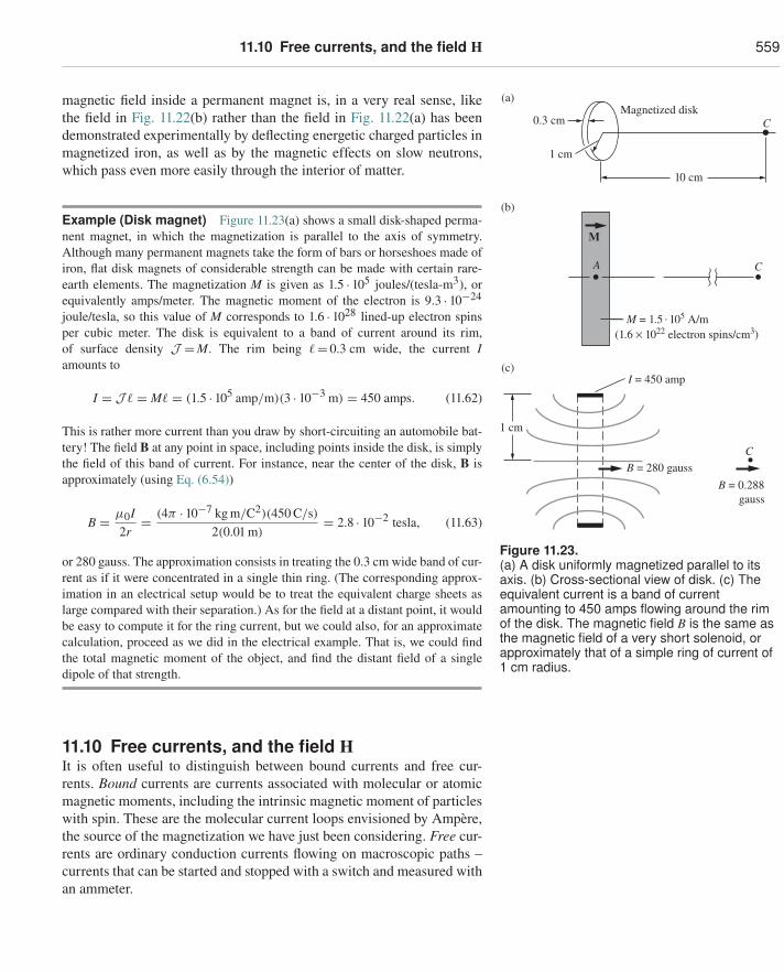
11.10 Free currents, and the field H 559
magnetic field inside a permanent magnet is, in a very real sense, likethe field in Fig. 11.22(b) rather than the field in Fig. 11.22(a) has beendemonstrated experimentally by deflecting energetic charged particles inmagnetized iron, as well as by the magnetic effects on slow neutrons,which pass even more easily through the interior of matter. 10 cm
CMagnetized disk
1 cm
0.3 cm
(a)
(c)
1 cm
I = 450 amp
B = 280 gaussB = 0.288 gauss
C
M
(1.6 × 10²² electron spins/cm3)M = 1.5 . 105 A/m
A C
(b)
Figure 11.23.(a) A disk uniformly magnetized parallel to itsaxis. (b) Cross-sectional view of disk. (c) Theequivalent current is a band of currentamounting to 450 amps flowing around the rimof the disk. The magnetic field B is the same asthe magnetic field of a very short solenoid, orapproximately that of a simple ring of current of1 cm radius.
Example (Disk magnet) Figure 11.23(a) shows a small disk-shaped perma-nent magnet, in which the magnetization is parallel to the axis of symmetry.Although many permanent magnets take the form of bars or horseshoes made ofiron, flat disk magnets of considerable strength can be made with certain rare-earth elements. The magnetization M is given as 1.5 · 105 joules/(tesla-m3), orequivalently amps/meter. The magnetic moment of the electron is 9.3 · 10−24
joule/tesla, so this value of M corresponds to 1.6 · 1028 lined-up electron spinsper cubic meter. The disk is equivalent to a band of current around its rim,of surface density J =M. The rim being �= 0.3 cm wide, the current Iamounts to
I = J � = M� = (1.5 · 105 amp/m)(3 · 10−3 m) = 450 amps. (11.62)
This is rather more current than you draw by short-circuiting an automobile bat-tery! The field B at any point in space, including points inside the disk, is simplythe field of this band of current. For instance, near the center of the disk, B isapproximately (using Eq. (6.54))
B = μ0I2r
= (4π · 10−7 kg m/C2)(450 C/s)2(0.01 m)
= 2.8 · 10−2 tesla, (11.63)
or 280 gauss. The approximation consists in treating the 0.3 cm wide band of cur-rent as if it were concentrated in a single thin ring. (The corresponding approx-imation in an electrical setup would be to treat the equivalent charge sheets aslarge compared with their separation.) As for the field at a distant point, it wouldbe easy to compute it for the ring current, but we could also, for an approximatecalculation, proceed as we did in the electrical example. That is, we could findthe total magnetic moment of the object, and find the distant field of a singledipole of that strength.
11.10 Free currents, and the field HIt is often useful to distinguish between bound currents and free cur-rents. Bound currents are currents associated with molecular or atomicmagnetic moments, including the intrinsic magnetic moment of particleswith spin. These are the molecular current loops envisioned by Ampère,the source of the magnetization we have just been considering. Free cur-rents are ordinary conduction currents flowing on macroscopic paths –currents that can be started and stopped with a switch and measured withan ammeter.
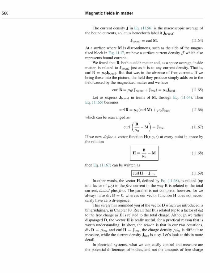
560 Magnetic fields in matter
The current density J in Eq. (11.56) is the macroscopic average ofthe bound currents, so let us henceforth label it Jbound:
Jbound = curl M. (11.64)
At a surface where M is discontinuous, such as the side of the magne-tized block in Fig. 11.17, we have a surface current density J which alsorepresents bound current.
We found that B, both outside matter and, as a space average, insidematter, is related to Jbound just as it is to any current density. That is,curl B = μ0Jbound. But that was in the absence of free currents. If webring these into the picture, the field they produce simply adds on to thefield caused by the magnetized matter and we have
curl B = μ0(Jbound + Jfree) = μ0Jtotal. (11.65)
Let us express Jbound in terms of M, through Eq. (11.64). ThenEq. (11.65) becomes
curl B = μ0(curl M) + μ0Jfree, (11.66)
which can be rearranged as
curl(
Bμ0
− M)= Jfree. (11.67)
If we now define a vector function H(x, y, z) at every point in space bythe relation
H ≡ Bμ0
− M (11.68)
then Eq. (11.67) can be written as
curl H = Jfree (11.69)
In other words, the vector H, defined by Eq. (11.68), is related (upto a factor of μ0) to the free current in the way B is related to the totalcurrent, bound plus free. The parallel is not complete, however, for wealways have div B = 0, whereas our vector function H does not neces-sarily have zero divergence.
This surely has reminded you of the vector D which we introduced, abit grudgingly, in Chapter 10. Recall that D is related (up to a factor of ε0)to the free charge as E is related to the total charge. Although we ratherdisparaged D, the vector H is really useful, for a practical reason that isworth understanding. In short, the reason is that in our two equations,div D = ρfree and curl H = Jfree, the charge density ρfree is difficult tomeasure, while the current density Jfree is easy. Let’s look at this in moredetail.
In electrical systems, what we can easily control and measure arethe potential differences of bodies, and not the amounts of free charge
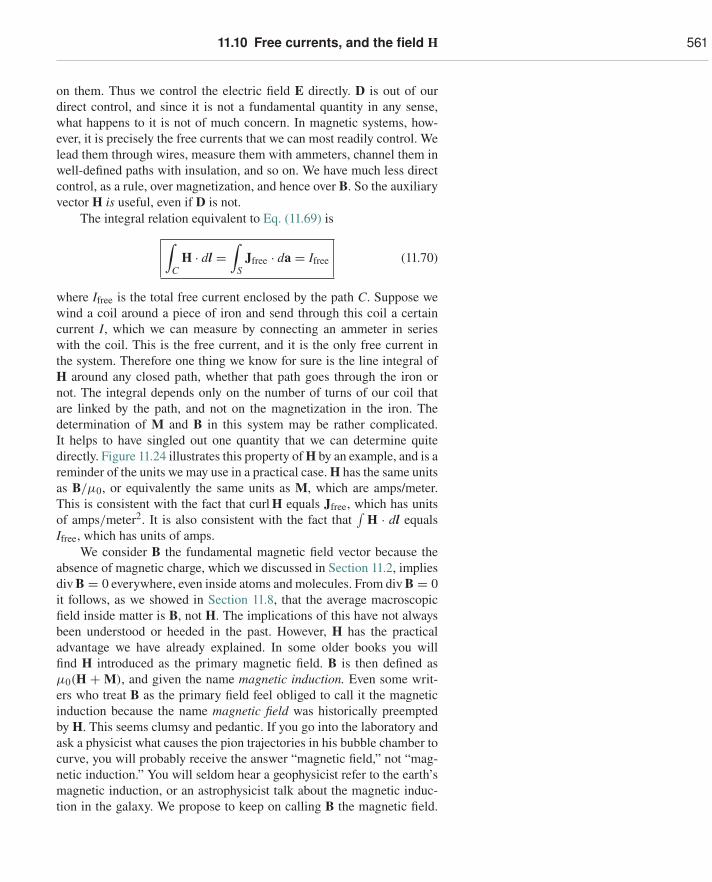
11.10 Free currents, and the field H 561
on them. Thus we control the electric field E directly. D is out of ourdirect control, and since it is not a fundamental quantity in any sense,what happens to it is not of much concern. In magnetic systems, how-ever, it is precisely the free currents that we can most readily control. Welead them through wires, measure them with ammeters, channel them inwell-defined paths with insulation, and so on. We have much less directcontrol, as a rule, over magnetization, and hence over B. So the auxiliaryvector H is useful, even if D is not.
The integral relation equivalent to Eq. (11.69) is∫C
H · dl =∫
SJfree · da = Ifree (11.70)
where Ifree is the total free current enclosed by the path C. Suppose wewind a coil around a piece of iron and send through this coil a certaincurrent I, which we can measure by connecting an ammeter in serieswith the coil. This is the free current, and it is the only free current inthe system. Therefore one thing we know for sure is the line integral ofH around any closed path, whether that path goes through the iron ornot. The integral depends only on the number of turns of our coil thatare linked by the path, and not on the magnetization in the iron. Thedetermination of M and B in this system may be rather complicated.It helps to have singled out one quantity that we can determine quitedirectly. Figure 11.24 illustrates this property of H by an example, and is areminder of the units we may use in a practical case. H has the same unitsas B/μ0, or equivalently the same units as M, which are amps/meter.This is consistent with the fact that curl H equals Jfree, which has unitsof amps/meter2. It is also consistent with the fact that
∫H · dl equals
Ifree, which has units of amps.We consider B the fundamental magnetic field vector because the
absence of magnetic charge, which we discussed in Section 11.2, impliesdiv B = 0 everywhere, even inside atoms and molecules. From div B = 0it follows, as we showed in Section 11.8, that the average macroscopicfield inside matter is B, not H. The implications of this have not alwaysbeen understood or heeded in the past. However, H has the practicaladvantage we have already explained. In some older books you willfind H introduced as the primary magnetic field. B is then defined asμ0(H + M), and given the name magnetic induction. Even some writ-ers who treat B as the primary field feel obliged to call it the magneticinduction because the name magnetic field was historically preemptedby H. This seems clumsy and pedantic. If you go into the laboratory andask a physicist what causes the pion trajectories in his bubble chamber tocurve, you will probably receive the answer “magnetic field,” not “mag-netic induction.” You will seldom hear a geophysicist refer to the earth’smagnetic induction, or an astrophysicist talk about the magnetic induc-tion in the galaxy. We propose to keep on calling B the magnetic field.
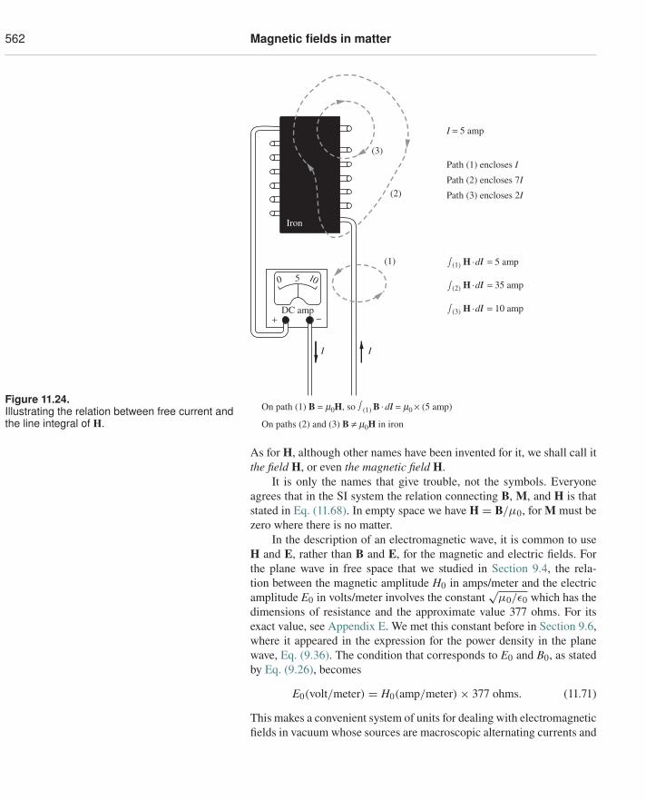
562 Magnetic fields in matter
Figure 11.24.Illustrating the relation between free current andthe line integral of H.
0 5
DC amp
10
I I
(1)
(2)
(3)
I = 5 amp
Path (1) encloses I
Path (2) encloses 7I
Path (3) encloses 2I
Iron
On path (1) B = m0H, so Ú (1) B . dl = m0 × (5 amp)
On paths (2) and (3) B ≠ m0H in iron
+ −
(1) H ·dl = 5 amp
(2) H ·dl = 35 amp
(3) H ·dl = 10 amp
Ú
Ú
Ú
As for H, although other names have been invented for it, we shall call itthe field H, or even the magnetic field H.
It is only the names that give trouble, not the symbols. Everyoneagrees that in the SI system the relation connecting B, M, and H is thatstated in Eq. (11.68). In empty space we have H = B/μ0, for M must bezero where there is no matter.
In the description of an electromagnetic wave, it is common to useH and E, rather than B and E, for the magnetic and electric fields. Forthe plane wave in free space that we studied in Section 9.4, the rela-tion between the magnetic amplitude H0 in amps/meter and the electricamplitude E0 in volts/meter involves the constant
√μ0/ε0 which has the
dimensions of resistance and the approximate value 377 ohms. For itsexact value, see Appendix E. We met this constant before in Section 9.6,where it appeared in the expression for the power density in the planewave, Eq. (9.36). The condition that corresponds to E0 and B0, as statedby Eq. (9.26), becomes
E0(volt/meter) = H0(amp/meter) × 377 ohms. (11.71)
This makes a convenient system of units for dealing with electromagneticfields in vacuum whose sources are macroscopic alternating currents and
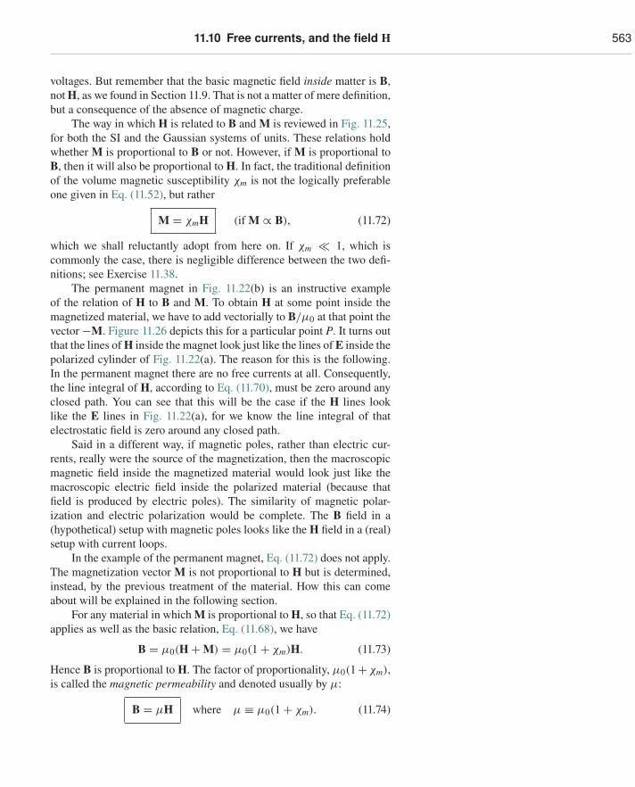
11.10 Free currents, and the field H 563
voltages. But remember that the basic magnetic field inside matter is B,not H, as we found in Section 11.9. That is not a matter of mere definition,but a consequence of the absence of magnetic charge.
The way in which H is related to B and M is reviewed in Fig. 11.25,for both the SI and the Gaussian systems of units. These relations holdwhether M is proportional to B or not. However, if M is proportional toB, then it will also be proportional to H. In fact, the traditional definitionof the volume magnetic susceptibility χm is not the logically preferableone given in Eq. (11.52), but rather
M = χmH (if M ∝ B), (11.72)
which we shall reluctantly adopt from here on. If χm � 1, which iscommonly the case, there is negligible difference between the two defi-nitions; see Exercise 11.38.
The permanent magnet in Fig. 11.22(b) is an instructive exampleof the relation of H to B and M. To obtain H at some point inside themagnetized material, we have to add vectorially to B/μ0 at that point thevector −M. Figure 11.26 depicts this for a particular point P. It turns outthat the lines of H inside the magnet look just like the lines of E inside thepolarized cylinder of Fig. 11.22(a). The reason for this is the following.In the permanent magnet there are no free currents at all. Consequently,the line integral of H, according to Eq. (11.70), must be zero around anyclosed path. You can see that this will be the case if the H lines looklike the E lines in Fig. 11.22(a), for we know the line integral of thatelectrostatic field is zero around any closed path.
Said in a different way, if magnetic poles, rather than electric cur-rents, really were the source of the magnetization, then the macroscopicmagnetic field inside the magnetized material would look just like themacroscopic electric field inside the polarized material (because thatfield is produced by electric poles). The similarity of magnetic polar-ization and electric polarization would be complete. The B field in a(hypothetical) setup with magnetic poles looks like the H field in a (real)setup with current loops.
In the example of the permanent magnet, Eq. (11.72) does not apply.The magnetization vector M is not proportional to H but is determined,instead, by the previous treatment of the material. How this can comeabout will be explained in the following section.
For any material in which M is proportional to H, so that Eq. (11.72)applies as well as the basic relation, Eq. (11.68), we have
B = μ0(H + M) = μ0(1 + χm)H. (11.73)
Hence B is proportional to H. The factor of proportionality, μ0(1+χm),is called the magnetic permeability and denoted usually by μ:
B = μH where μ ≡ μ0(1 + χm). (11.74)
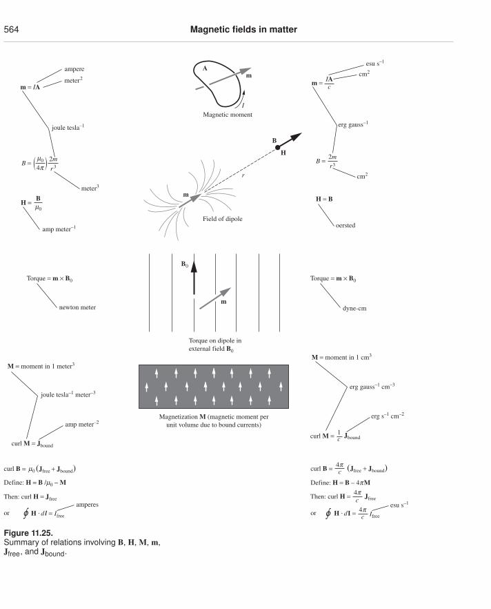
564 Magnetic fields in matter
m =
esu s–1
erg gauss–1
oersted
newton meter
cm2
cm2
meter3
cIA
Magnetization M (magnetic moment perunit volume due to bound currents)
B =
H = B
amp meter–1
H =
r32m
m0
B
m = IA
ampere
joule tesla–1
meter2
B =4pm0 2m
r3
joule tesla–1 meter–3
amp meter–2
curl M = Jbound
M = moment in 1 meter3
dyne-cm
Torque = m × B0Torque = m × B0
erg gauss–1 cm–3
erg s–1 cm–2
curl M = Jbound
M = moment in 1 cm3
c1
esu s–1
Define: H = B – 4pM
Then: curl H =
or H . dI =
Jfree
curl B = (Jfree + Jbound)c4p
c4p
c4p
Ifree
amperes
Define: H = B /m0 − M
Then: curl H = Jfree
curl B = (Jfree + Jbound)m0
or H . d l = Ifree
Am
Magnetic momentI
B
H
m
r
Field of dipole
Torque on dipole inexternal field B0
B0
m
Figure 11.25.Summary of relations involving B, H, M, m,Jfree, and Jbound.
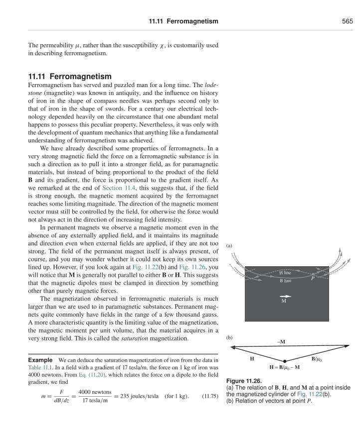
11.11 Ferromagnetism 565
The permeability μ, rather than the susceptibility χ , is customarily usedin describing ferromagnetism.
11.11 FerromagnetismFerromagnetism has served and puzzled man for a long time. The lode-stone (magnetite) was known in antiquity, and the influence on historyof iron in the shape of compass needles was perhaps second only tothat of iron in the shape of swords. For a century our electrical tech-nology depended heavily on the circumstance that one abundant metalhappens to possess this peculiar property. Nevertheless, it was only withthe development of quantum mechanics that anything like a fundamentalunderstanding of ferromagnetism was achieved.
We have already described some properties of ferromagnets. In avery strong magnetic field the force on a ferromagnetic substance is insuch a direction as to pull it into a stronger field, as for paramagneticmaterials, but instead of being proportional to the product of the fieldB and its gradient, the force is proportional to the gradient itself. Aswe remarked at the end of Section 11.4, this suggests that, if the fieldis strong enough, the magnetic moment acquired by the ferromagnetreaches some limiting magnitude. The direction of the magnetic momentvector must still be controlled by the field, for otherwise the force wouldnot always act in the direction of increasing field intensity.
In permanent magnets we observe a magnetic moment even in theabsence of any externally applied field, and it maintains its magnitudeand direction even when external fields are applied, if they are not toostrong. The field of the permanent magnet itself is always present, ofcourse, and you may wonder whether it could not keep its own sourceslined up. However, if you look again at Fig. 11.22(b) and Fig. 11.26, youwill notice that M is generally not parallel to either B or H. This suggeststhat the magnetic dipoles must be clamped in direction by somethingother than purely magnetic forces.
H
(b)
(a)
B/m0
−M
H = B/m0 − M
H lineP
M
B line
Figure 11.26.(a) The relation of B, H, and M at a point insidethe magnetized cylinder of Fig. 11.22(b).(b) Relation of vectors at point P.
The magnetization observed in ferromagnetic materials is muchlarger than we are used to in paramagnetic substances. Permanent mag-nets quite commonly have fields in the range of a few thousand gauss.A more characteristic quantity is the limiting value of the magnetization,the magnetic moment per unit volume, that the material acquires in avery strong field. This is called the saturation magnetization.
Example We can deduce the saturation magnetization of iron from the data inTable 11.1. In a field with a gradient of 17 tesla/m, the force on 1 kg of iron was4000 newtons. From Eq. (11.20), which relates the force on a dipole to the fieldgradient, we find
m = FdB/dz
= 4000 newtons17 tesla/m
= 235 joules/tesla (for 1 kg). (11.75)
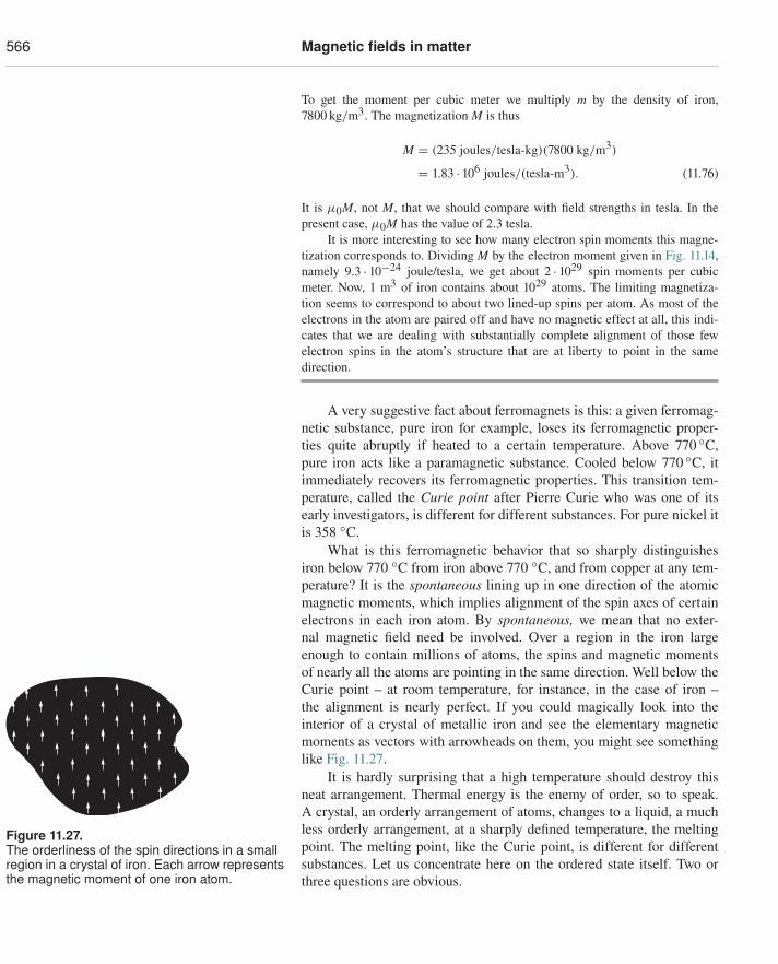
566 Magnetic fields in matter
To get the moment per cubic meter we multiply m by the density of iron,7800 kg/m3. The magnetization M is thus
M = (235 joules/tesla-kg)(7800 kg/m3)
= 1.83 · 106 joules/(tesla-m3). (11.76)
It is μ0M, not M, that we should compare with field strengths in tesla. In thepresent case, μ0M has the value of 2.3 tesla.
It is more interesting to see how many electron spin moments this magne-tization corresponds to. Dividing M by the electron moment given in Fig. 11.14,namely 9.3 · 10−24 joule/tesla, we get about 2 · 1029 spin moments per cubicmeter. Now, 1 m3 of iron contains about 1029 atoms. The limiting magnetiza-tion seems to correspond to about two lined-up spins per atom. As most of theelectrons in the atom are paired off and have no magnetic effect at all, this indi-cates that we are dealing with substantially complete alignment of those fewelectron spins in the atom’s structure that are at liberty to point in the samedirection.
A very suggestive fact about ferromagnets is this: a given ferromag-netic substance, pure iron for example, loses its ferromagnetic proper-ties quite abruptly if heated to a certain temperature. Above 770 ◦C,pure iron acts like a paramagnetic substance. Cooled below 770 ◦C, itimmediately recovers its ferromagnetic properties. This transition tem-perature, called the Curie point after Pierre Curie who was one of itsearly investigators, is different for different substances. For pure nickel itis 358 ◦C.
What is this ferromagnetic behavior that so sharply distinguishesiron below 770 ◦C from iron above 770 ◦C, and from copper at any tem-perature? It is the spontaneous lining up in one direction of the atomicmagnetic moments, which implies alignment of the spin axes of certainelectrons in each iron atom. By spontaneous, we mean that no exter-nal magnetic field need be involved. Over a region in the iron largeenough to contain millions of atoms, the spins and magnetic momentsof nearly all the atoms are pointing in the same direction. Well below theCurie point – at room temperature, for instance, in the case of iron –the alignment is nearly perfect. If you could magically look into theinterior of a crystal of metallic iron and see the elementary magneticmoments as vectors with arrowheads on them, you might see somethinglike Fig. 11.27.
Figure 11.27.The orderliness of the spin directions in a smallregion in a crystal of iron. Each arrow representsthe magnetic moment of one iron atom.
It is hardly surprising that a high temperature should destroy thisneat arrangement. Thermal energy is the enemy of order, so to speak.A crystal, an orderly arrangement of atoms, changes to a liquid, a muchless orderly arrangement, at a sharply defined temperature, the meltingpoint. The melting point, like the Curie point, is different for differentsubstances. Let us concentrate here on the ordered state itself. Two orthree questions are obvious.
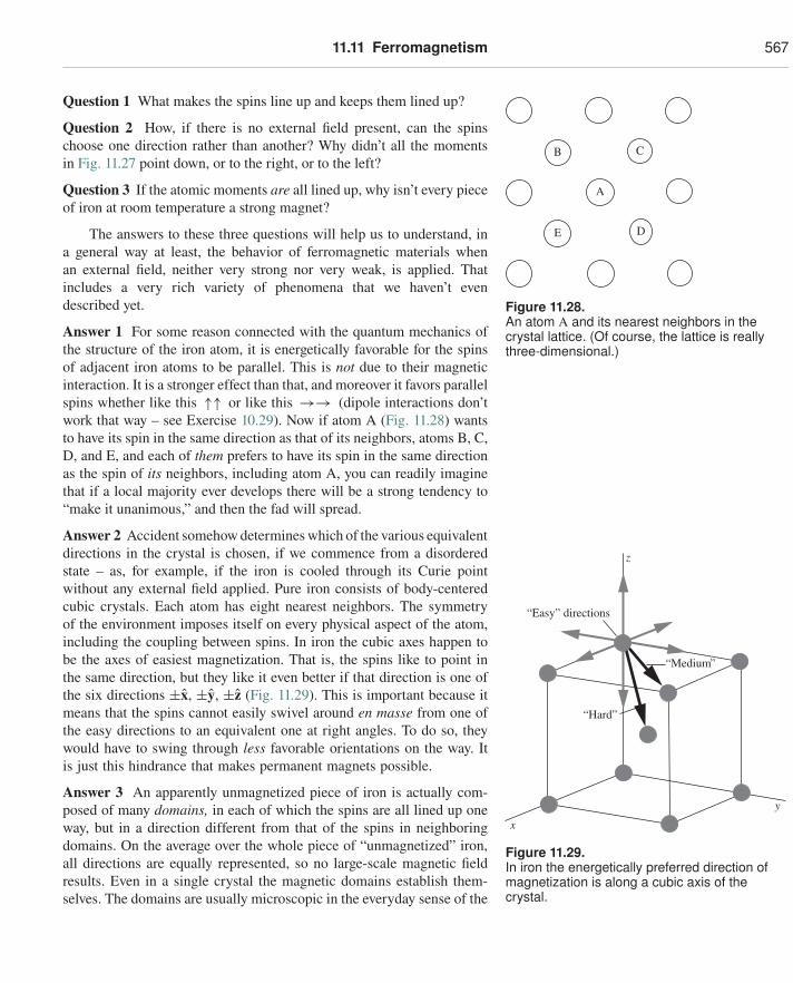
11.11 Ferromagnetism 567
Question 1 What makes the spins line up and keeps them lined up?
Question 2 How, if there is no external field present, can the spinschoose one direction rather than another? Why didn’t all the momentsin Fig. 11.27 point down, or to the right, or to the left?
Question 3 If the atomic moments are all lined up, why isn’t every pieceof iron at room temperature a strong magnet?
A
B
E D
C
Figure 11.28.An atom A and its nearest neighbors in thecrystal lattice. (Of course, the lattice is reallythree-dimensional.)
The answers to these three questions will help us to understand, ina general way at least, the behavior of ferromagnetic materials whenan external field, neither very strong nor very weak, is applied. Thatincludes a very rich variety of phenomena that we haven’t evendescribed yet.
Answer 1 For some reason connected with the quantum mechanics ofthe structure of the iron atom, it is energetically favorable for the spinsof adjacent iron atoms to be parallel. This is not due to their magneticinteraction. It is a stronger effect than that, and moreover it favors parallelspins whether like this ↑↑ or like this →→ (dipole interactions don’twork that way – see Exercise 10.29). Now if atom A (Fig. 11.28) wantsto have its spin in the same direction as that of its neighbors, atoms B, C,D, and E, and each of them prefers to have its spin in the same directionas the spin of its neighbors, including atom A, you can readily imaginethat if a local majority ever develops there will be a strong tendency to“make it unanimous,” and then the fad will spread.
Answer 2 Accident somehow determines which of the various equivalentdirections in the crystal is chosen, if we commence from a disorderedstate – as, for example, if the iron is cooled through its Curie pointwithout any external field applied. Pure iron consists of body-centeredcubic crystals. Each atom has eight nearest neighbors. The symmetryof the environment imposes itself on every physical aspect of the atom,including the coupling between spins. In iron the cubic axes happen tobe the axes of easiest magnetization. That is, the spins like to point inthe same direction, but they like it even better if that direction is one ofthe six directions ±x, ±y, ±z (Fig. 11.29). This is important because itmeans that the spins cannot easily swivel around en masse from one ofthe easy directions to an equivalent one at right angles. To do so, theywould have to swing through less favorable orientations on the way. Itis just this hindrance that makes permanent magnets possible.
“Medium”
“Hard”
“Easy” directions
z
x
y
Figure 11.29.In iron the energetically preferred direction ofmagnetization is along a cubic axis of thecrystal.
Answer 3 An apparently unmagnetized piece of iron is actually com-posed of many domains, in each of which the spins are all lined up oneway, but in a direction different from that of the spins in neighboringdomains. On the average over the whole piece of “unmagnetized” iron,all directions are equally represented, so no large-scale magnetic fieldresults. Even in a single crystal the magnetic domains establish them-selves. The domains are usually microscopic in the everyday sense of the
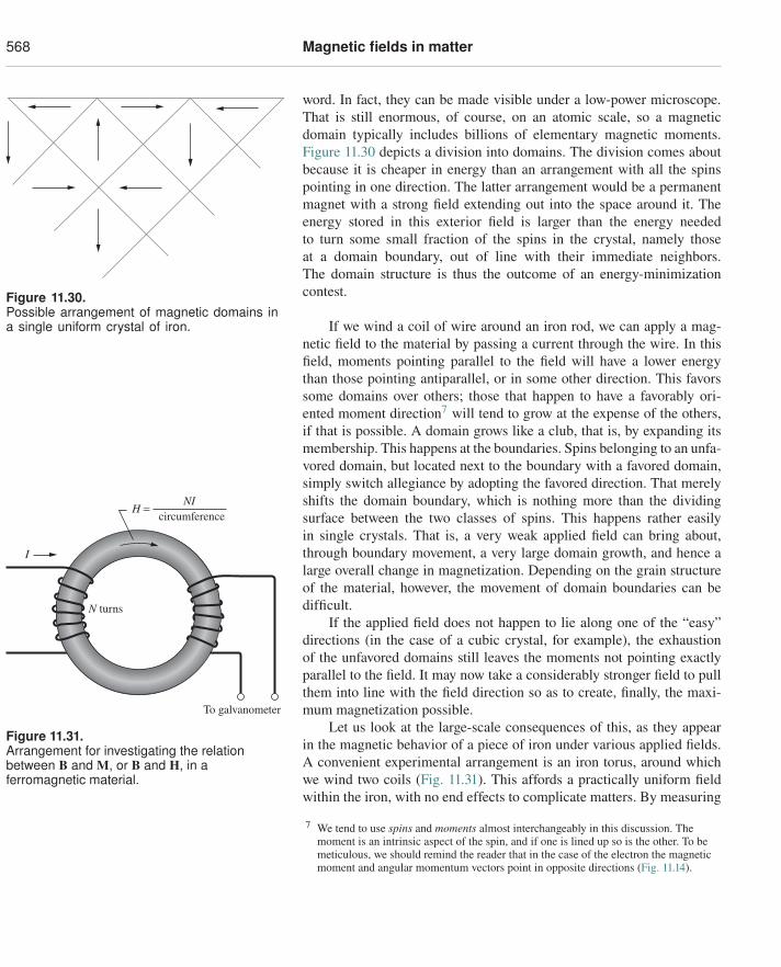
568 Magnetic fields in matter
word. In fact, they can be made visible under a low-power microscope.That is still enormous, of course, on an atomic scale, so a magneticdomain typically includes billions of elementary magnetic moments.Figure 11.30 depicts a division into domains. The division comes about
Figure 11.30.Possible arrangement of magnetic domains ina single uniform crystal of iron.
because it is cheaper in energy than an arrangement with all the spinspointing in one direction. The latter arrangement would be a permanentmagnet with a strong field extending out into the space around it. Theenergy stored in this exterior field is larger than the energy neededto turn some small fraction of the spins in the crystal, namely thoseat a domain boundary, out of line with their immediate neighbors.The domain structure is thus the outcome of an energy-minimizationcontest.
If we wind a coil of wire around an iron rod, we can apply a mag-netic field to the material by passing a current through the wire. In thisfield, moments pointing parallel to the field will have a lower energythan those pointing antiparallel, or in some other direction. This favorssome domains over others; those that happen to have a favorably ori-ented moment direction7 will tend to grow at the expense of the others,if that is possible. A domain grows like a club, that is, by expanding itsmembership. This happens at the boundaries. Spins belonging to an unfa-vored domain, but located next to the boundary with a favored domain,simply switch allegiance by adopting the favored direction. That merelyshifts the domain boundary, which is nothing more than the dividingsurface between the two classes of spins. This happens rather easilyin single crystals. That is, a very weak applied field can bring about,through boundary movement, a very large domain growth, and hence alarge overall change in magnetization. Depending on the grain structureof the material, however, the movement of domain boundaries can bedifficult.
circumference
To galvanometer
I
H =NI
N turns
Figure 11.31.Arrangement for investigating the relationbetween B and M, or B and H, in aferromagnetic material.
If the applied field does not happen to lie along one of the “easy”directions (in the case of a cubic crystal, for example), the exhaustionof the unfavored domains still leaves the moments not pointing exactlyparallel to the field. It may now take a considerably stronger field to pullthem into line with the field direction so as to create, finally, the maxi-mum magnetization possible.
Let us look at the large-scale consequences of this, as they appearin the magnetic behavior of a piece of iron under various applied fields.A convenient experimental arrangement is an iron torus, around whichwe wind two coils (Fig. 11.31). This affords a practically uniform fieldwithin the iron, with no end effects to complicate matters. By measuring
7 We tend to use spins and moments almost interchangeably in this discussion. Themoment is an intrinsic aspect of the spin, and if one is lined up so is the other. To bemeticulous, we should remind the reader that in the case of the electron the magneticmoment and angular momentum vectors point in opposite directions (Fig. 11.14).
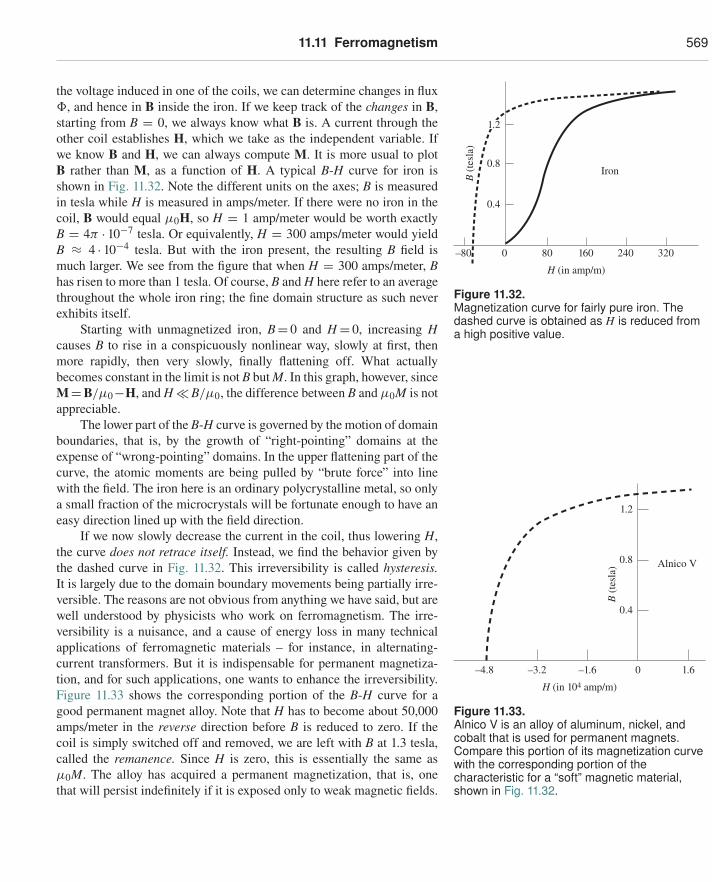
11.11 Ferromagnetism 569
the voltage induced in one of the coils, we can determine changes in flux�, and hence in B inside the iron. If we keep track of the changes in B,starting from B = 0, we always know what B is. A current through theother coil establishes H, which we take as the independent variable. Ifwe know B and H, we can always compute M. It is more usual to plotB rather than M, as a function of H. A typical B-H curve for iron isshown in Fig. 11.32. Note the different units on the axes; B is measuredin tesla while H is measured in amps/meter. If there were no iron in thecoil, B would equal μ0H, so H = 1 amp/meter would be worth exactlyB = 4π · 10−7 tesla. Or equivalently, H = 300 amps/meter would yieldB ≈ 4 · 10−4 tesla. But with the iron present, the resulting B field ismuch larger. We see from the figure that when H = 300 amps/meter, Bhas risen to more than 1 tesla. Of course, B and H here refer to an averagethroughout the whole iron ring; the fine domain structure as such neverexhibits itself.
Iron
H (in amp/m)
B (t
esla
)
0.4
0–80 80 160 240 320
0.8
1.2
Figure 11.32.Magnetization curve for fairly pure iron. Thedashed curve is obtained as H is reduced froma high positive value.Starting with unmagnetized iron, B= 0 and H = 0, increasing H
causes B to rise in a conspicuously nonlinear way, slowly at first, thenmore rapidly, then very slowly, finally flattening off. What actuallybecomes constant in the limit is not B but M. In this graph, however, sinceM=B/μ0−H, and H �B/μ0, the difference between B and μ0M is notappreciable.
The lower part of the B-H curve is governed by the motion of domainboundaries, that is, by the growth of “right-pointing” domains at theexpense of “wrong-pointing” domains. In the upper flattening part of thecurve, the atomic moments are being pulled by “brute force” into linewith the field. The iron here is an ordinary polycrystalline metal, so onlya small fraction of the microcrystals will be fortunate enough to have aneasy direction lined up with the field direction.
H (in 104 amp/m)
Alnico V
B (t
esla
)
1.2
0.8
0.4
1.6–1.6–3.2–4.8 0
Figure 11.33.Alnico V is an alloy of aluminum, nickel, andcobalt that is used for permanent magnets.Compare this portion of its magnetization curvewith the corresponding portion of thecharacteristic for a “soft” magnetic material,shown in Fig. 11.32.
If we now slowly decrease the current in the coil, thus lowering H,the curve does not retrace itself. Instead, we find the behavior given bythe dashed curve in Fig. 11.32. This irreversibility is called hysteresis.It is largely due to the domain boundary movements being partially irre-versible. The reasons are not obvious from anything we have said, but arewell understood by physicists who work on ferromagnetism. The irre-versibility is a nuisance, and a cause of energy loss in many technicalapplications of ferromagnetic materials – for instance, in alternating-current transformers. But it is indispensable for permanent magnetiza-tion, and for such applications, one wants to enhance the irreversibility.Figure 11.33 shows the corresponding portion of the B-H curve for agood permanent magnet alloy. Note that H has to become about 50,000amps/meter in the reverse direction before B is reduced to zero. If thecoil is simply switched off and removed, we are left with B at 1.3 tesla,called the remanence. Since H is zero, this is essentially the same asμ0M. The alloy has acquired a permanent magnetization, that is, onethat will persist indefinitely if it is exposed only to weak magnetic fields.
570 Magnetic fields in matter
All the information that is stored on magnetic tapes and disks owes itspermanence to this physical phenomenon.
11.12 ApplicationsLodestone is magnetite (which is a type of iron oxide) that has been mag-netized. Most magnetite isn’t lodestone; the earth’s magnetic field is tooweak to create the observed magnetization. (And additionally, a partic-ular crystal structure in the magnetite is needed.) A much stronger fieldis required, and this is the field produced by the brief but large electriccurrent in a lightning strike. So without lightning, there would be nomagnetic compasses, and the explorers throughout history would havehad a much more difficult time!
Red pigments in paint often contain iron oxide grains. When thepaint is wet, the grains’ magnetic dipole moments are free to rotate andalign themselves with the earth’s magnetic field. But when the paintdries, they are locked in place. The direction of the dipole moments ina painting therefore gives the direction of the earth’s magnetic field atthe time the painting was made. By studying paintings whose positionsare fixed, such as murals, we can gather information on how the earth’smagnetic field has changed over time, assuming that the creation datesare known. (This doesn’t work with framed paintings that have beenmoved around, or with murals that have undergone restoration!) Con-versely, knowing the direction of the dipoles in a given painting can helpdetermine the creation date; this can be very useful for archaeologicalpurposes.
A common application of ferromagnetic materials is the magnifica-tion of the magnetic field from a coil of wire. If a coil is wrapped around aferromagnetic core (usually iron-based), the coil’s magnetic field causesthe spins in the core material to align with the field, thereby producinga much larger field than the coil would produce by itself. The magnifi-cation factor (which is just the relative permeability, μ/μ0) depends onvarious things, but for ferromagnetic materials it can be 100 or 1000, oreven larger. This magnification effect is used in the electromagnets inrelays, circuit breakers, junkyard magnets, and many other devices (seeSection 6.10).
Many data storage devices, from cassette tapes to computer harddisks to credit cards, rely on the existence of ferromagnetic materials.(There are many other types of storage devices too. For example, CDsand DVDs operate by reflecting laser light off tiny pits in a plastic diskcoated with aluminum. And flash memory makes use of a special kindof transistor.) A cassette tape (RIP) was the dominant format for musicrecording in the 1980s. The cassette consists of a long plastic tape coatedwith iron oxide, wound around two small reels. The read/write head isa tiny electromagnet. In the writing (recording) mode, a current passesthrough the coil of the electromagnet, producing a magnetic field that
11.12 Applications 571
aligns the magnetic dipoles on the tape as it moves past. The tape there-fore encodes the information in the current in the original signal.8 Con-versely, in the reading (playback) mode, the magnetic field of the dipolesin the tape induces a current in the electromagnet as the magneticdomains in the tape move past. This induced current contains the sameinformation as what is on the tape. It can then be amplified and sent to aspeaker.
A computer hard disk operates under the same general principle as acassette tape, although there are some differences. Instead of a long tape,the hard disk, as the name suggests, takes the form of a disk on whichthe magnetic data is encoded in very narrow circular tracks. The mag-netic domains are much smaller, and the average linear speed relativeto the read/write head is much larger. The information at a given loca-tion on a disk can be accessed much more quickly than on a linear tape,because there is no need to run through the tape to gain access to a givenpoint. Another important difference is that the cassette tape is an analogdevice, whereas the hard disk is a digital one. That is, as the current in thecassette’s write-head electromagnet changes smoothly, the induced mag-netization of the tape also changes smoothly, and this smoothly varyingfunction contains the desired information. But in a hard disk, the mag-netization is “all or nothing”; the write-head electromagnet either doesnothing or completely saturates a magnetic domain. The abrupt changes(or lack thereof) in the magnetization are what is detected by the readhead. So the information that comes out is just a string of yes’s or no’s,that is, 1’s or 0’s. In modern computers the reading is done with a sep-arate magnetoresistive head, whose resistance depends on the magneticfield from the disk. This type of head is better able to read the tiny mag-netic features on the disk. As incredibly useful as magnetic data stor-age is, beware that it isn’t permanent. Hard-disk data can degrade onthe order of 10 years. If you really want your data to last, you can useCDs that are made with a layer of gold. These are designed to last 300years, although the supporting hardware will certainly be replaced longbefore then.
As discussed in Exercise 11.25, magnetic bacteria contain crystalsof iron (often in the form of magnetite) that keep the bacteria alignedwith the earth’s magnetic field. The alignment is passive, that is, it wouldwork even if a bacterium were dead. The point of the alignment is notto indicate which way is north, but rather which way is down. Exceptnear the magnetic equator, the earth’s magnetic field is inclined verti-cally. In the simplest scenario, bacteria follow the downward field linesto the oxygen-deprived regions (which they like) in the mud. (However,
8 The process is complicated due to hysteresis; the magnetization tends to keep itsoriginal value and doesn’t respond linearly to the applied magnetic field. This isremedied by adding a bias signal to the original signal. The purpose of this bias signal(whose frequency is high – usually around 100 kHz) is basically to average out thepositive and negative effects of the hysteresis.
572 Magnetic fields in matter
other mechanisms allow them also to seek out oxygen-deprived layers ofwater higher up.) The orientation of the magnetization of the crystals isopposite in bacteria in the northern and southern hemispheres, so theyall do indeed swim downward. If a bacterium is transported to the otherhemisphere, it will swim upward. Near the magnetic equator, there areroughly equal numbers of each type, and presumably another navigationmechanism takes over.
Many other creatures, such as homing pigeons, sea turtles, and rain-bow trout, also use the earth’s magnetic field to navigate. The exactmechanism isn’t known, but with pigeons, for example, the beak mostlikely contains tiny crystals of magnetite that transmit a signal to thebrain. The mechanism differs from the one in bacteria in that it is active(that is, a signal needs to be sent) rather than passive; in bacteria thetorque on the magnetic crystals simply rotates the bacteria. Also, forpigeons the purpose of the magnetite is to indicate which way is north(or south, etc.), and not which way is down, as in the case of bacteria. Abacterium wants to make a beeline along a magnetic field line to the mud,whereas a pigeon has no great desire to make a beeline for the ground!
A ferrofluid consists of tiny (on the order of a nanometer) ferro-magnetic particles suspended in a fluid. A surfactant (discussed in Sec-tion 10.16) keeps the particles evenly distributed in the fluid, so that theydon’t all clump together in the presence of a magnetic field. When amagnetic field is applied, a ferrofluid can take on bizarre shapes, withspikes and valleys brought about by the complicated balancing of mag-netic, gravitational, and surface-tension forces. Aside from making coolshapes, ferrofluids have many useful applications – in magnetic reso-nance imaging, as seals in devices with rotating parts, and as a means ofheat transfer. The ability to transfer heat efficiently is due to the temper-ature dependence of the magnetic susceptibility. In a speaker, for exam-ple, heat is generated near the voice coil, and the hotter ferrofluid (witha smaller magnetization than the colder ferrofluid) will experience asmaller magnetic force, and can therefore be displaced toward a heat sink.
Magnetorheological fluids are similar to ferrofluids, except that themagnetic particles are larger. When a magnetic field is applied, the par-ticles tend to line up along the field lines, which increases the viscosityin the orthogonal direction. One application is in shock absorbers, wherean electromagnet constantly adjusts the stiffness of the fluid, dependingon the instantaneous road condition.
If you hold one permanent magnet above another, you can pick upthe bottom one. So the magnetic force from the top magnet does workon the bottom magnet. However, isn’t it the case that magnetic forces dono work, because the qv × B Lorentz force is always perpendicular tothe velocity v? Actually, no. Magnetic forces can do work in some cases.More precisely, the no-magnetic-work conclusion holds only if the forceis governed by the qv × B Lorentz force law, which applies to pointcharges moving through space. This force law has nothing to do with
Chapter summary 573
the force on a magnetic dipole arising from a quantum mechanical spin,which cannot be viewed as a tiny current loop. The force on a dipoleis instead given by ∇(m ·B). Although we motivated this force law inSection 11.4 by considering a current loop, it can in fact be derived fromfundamental physical principles (relativity, quantum mechanics, and afew other things), with no reference to moving charges or the Lorentzforce. The ∇(m ·B) force has a potential energy associated with it, andthe change in this potential energy equals the work done on the dipole.If you picked up an actual current ring by holding another current ringabove it, then, as the bottom ring moved upward, you can show thatthe current in it would decrease (which the spin of an electron can’tdo). A battery (or something) would be needed to maintain the cur-rent, and this battery would be the agency doing the work, because theno-magnetic-work conclusion would hold in this case. See Problem 7.2for a related setup and a detailed discussion of why the magnetic Lorentzforce ends up doing zero net work on moving charges.
Most permanent magnets are made of a combination of iron andother elements, such as nickel, cobalt, and oxygen. But in recent yearspermanent magnets made of rare-earth elements such as neodymiumand samarium (combined with other more common elements) have comeinto wide usage. Rare-earth magnets are generally a bit stronger thaniron-based ones. The fields are often in the 1–1.5 tesla range, whereas thefield of an iron magnet is usually less than 0.5 tesla (although it can reach1 tesla for some types). Additionally, the crystal structure of a rare-earthmagnet is highly anisotropic. As discussed in the answer to Question 2 inSection 11.11, this means that it is difficult to change the direction of theindividual magnetic dipole moments. It is therefore difficult to demagne-tize a rare-earth magnet. Rare-earth magnets have replaced standard ironmagnets in many electronic devices.
CHAPTER SUMMARY• There are three types of magnetism. (1) Diamagnetism arises from
the orbital angular momentum of electrons; a diamagnetic momentpoints antiparallel to the external magnetic field. (2) Paramagnetismarises from the spin angular momentum of electrons; a paramagneticmoment points parallel to the external magnetic field (in an averagesense). (3) Ferromagnetism also arises from the spin angular momen-tum of electrons, but the interactions involved can be explained onlywith quantum mechanics; a ferromagnetic moment can exist in theabsence of an external magnetic field.
• The force on a diamagnetic material points in the direction of decreas-ing magnetic field strength, while the force on a paramagnetic materialpoints in the direction of increasing magnetic field strength. The force
574 Magnetic fields in matter
on a ferromagnetic material can point either way, but in a field strongenough to wash out any initial magnetization that may have existed,the force points in the direction of increasing magnetic field strength.
• Unlike electric fields, magnetic fields are caused by currents, not poles.The absence of magnetic poles can be stated as div B = 0.
• The magnetic moment of a current loop is m = Ia. The vector poten-tial due to the loop can be written as A = (μ0/4π)m× r/r2, and themagnetic dipole field in spherical coordinates is
Br = μ0m2πr3 cos θ , Bθ = μ0m
4πr3 sin θ . (11.77)
• The force on a magnetic dipole is F = ∇(m ·B). This takes a differentform compared with the force on an electric dipole.
• The magnetic moment due to the orbital motion of an electron is m =−(e/2me)L, where L is the orbital angular momentum. The diamag-netic moment induced in an external field B is m = −(e2r2/4me)B.
• Electrons also contain spin angular momentum and a spin dipolemoment. Paramagnetism arises from the (partial) alignment of thespins. The torque on a dipole moment is N = m × B.
• In many cases the diamagnetic and paramagnetic dipole magnetiza-tions M are proportional to the applied external field B. The magneticsusceptibility can be defined by M = χmB/μ0, although a differentdefinition in terms of H (see below) is the conventional one. The para-magnetic susceptibility is given approximately by χpm = μ0Nm2/kT .
• The magnetic field due to a uniformly magnetized slab is equivalent,both inside and outside, to the magnetic field due to a current on the“side” surface with density J = M. If the magnetization is not con-stant, then we more generally have J = curl M.
• The magnetic field H is defined by
H ≡ Bμ0
− M. (11.78)
This field satisfies
curl H = Jfree ⇐⇒∫
CH · dl = Ifree. (11.79)
If M is proportional to B, then the accepted definition of the magneticsusceptibility is M = χmH. The magnetic permeability is defined by
B = μH, where μ ≡ μ0(1 + χm). (11.80)
• Like paramagnetism, ferromagnetism arises from the spin angularmomentum of electrons, but in a more inherently quantum-mechanicalway that allows magnetization to exist even in the absence of an exter-nal magnetic field. A ferromagnetic material is divided into differentdomains where the spins are aligned. Increasing the external magneticfield can shift the boundaries of these domains. However, this processis not exactly reversible – an effect called hysteresis.
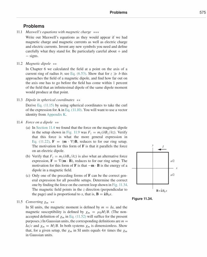
Problems 575
Problems11.1 Maxwell’s equations with magnetic charge ***
Write out Maxwell’s equations as they would appear if we hadmagnetic charge and magnetic currents as well as electric chargeand electric currents. Invent any new symbols you need and definecarefully what they stand for. Be particularly careful about + and− signs.
11.2 Magnetic dipole **In Chapter 6 we calculated the field at a point on the axis of acurrent ring of radius b; see Eq. (6.53). Show that for z � b thisapproaches the field of a magnetic dipole, and find how far out onthe axis one has to go before the field has come within 1 percentof the field that an infinitesimal dipole of the same dipole momentwould produce at that point.
11.3 Dipole in spherical coordinates **Derive Eq. (11.15) by using spherical coordinates to take the curlof the expression for A in Eq. (11.10). You will want to use a vectoridentity from Appendix K.
11.4 Force on a dipole **(a) In Section 11.4 we found that the force on the magnetic dipole
in the setup shown in Fig. 11.9 was Fz = mz(∂Bz/∂z). Verifythat this force is what the more general expression inEq. (11.22), F = (m · ∇)B, reduces to for our ring setup.The motivation for this form of F is that it parallels the forceon an electric dipole.
(b) Verify that Fz = mz(∂Bz/∂z) is also what an alternative forceexpression, F = ∇(m · B), reduces to for our ring setup. Themotivation for this form of F is that −m · B is the energy of adipole in a magnetic field.
I
x
a/2
a/2
y
B = z B0 x
Figure 11.34.
(c) Only one of the preceding forms of F can be the correct gen-eral expression for all possible setups. Determine the correctone by finding the force on the current loop shown in Fig. 11.34.The magnetic field points in the z direction (perpendicular tothe page) and is proportional to x, that is, B = zB0x.
11.5 Converting χm **In SI units, the magnetic moment is defined by m = Ia, and themagnetic susceptibility is defined by χm = μ0M/B. (The non-accepted definition of χm in Eq. (11.52) will suffice for the presentpurposes.) In Gaussian units, the corresponding definitions are m =Ia/c and χm = M/B. In both systems χm is dimensionless. Showthat, for a given setup, the χm in SI units equals 4π times the χmin Gaussian units.
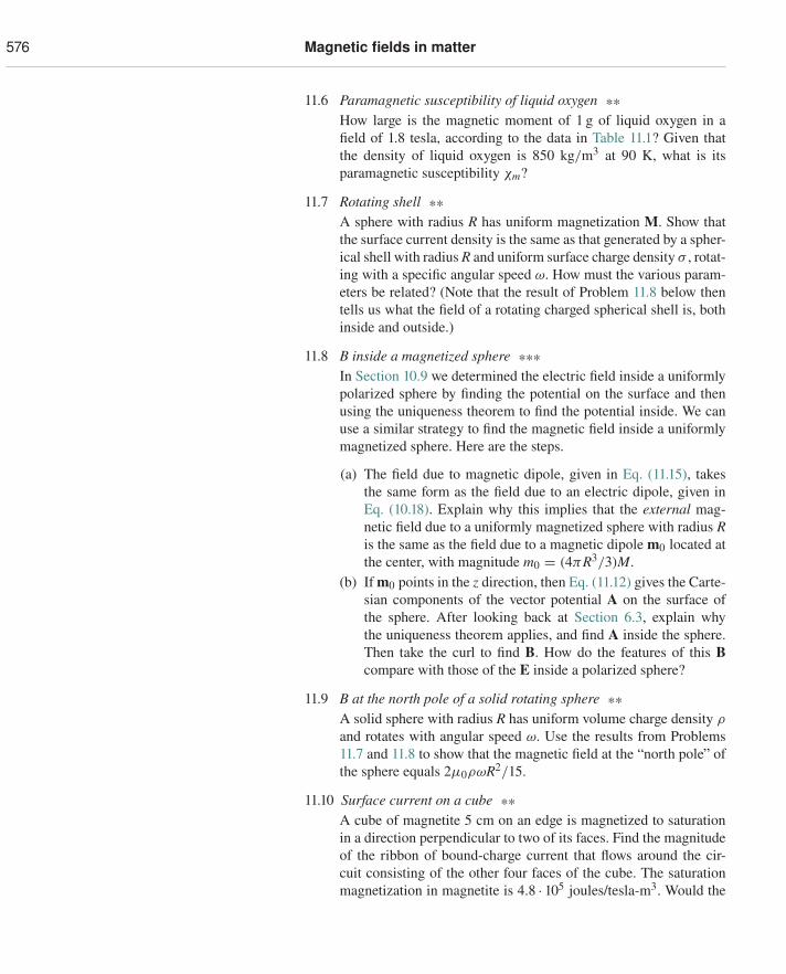
576 Magnetic fields in matter
11.6 Paramagnetic susceptibility of liquid oxygen **How large is the magnetic moment of 1 g of liquid oxygen in afield of 1.8 tesla, according to the data in Table 11.1? Given thatthe density of liquid oxygen is 850 kg/m3 at 90 K, what is itsparamagnetic susceptibility χm?
11.7 Rotating shell **A sphere with radius R has uniform magnetization M. Show thatthe surface current density is the same as that generated by a spher-ical shell with radius R and uniform surface charge density σ , rotat-ing with a specific angular speed ω. How must the various param-eters be related? (Note that the result of Problem 11.8 below thentells us what the field of a rotating charged spherical shell is, bothinside and outside.)
11.8 B inside a magnetized sphere ***In Section 10.9 we determined the electric field inside a uniformlypolarized sphere by finding the potential on the surface and thenusing the uniqueness theorem to find the potential inside. We canuse a similar strategy to find the magnetic field inside a uniformlymagnetized sphere. Here are the steps.
(a) The field due to magnetic dipole, given in Eq. (11.15), takesthe same form as the field due to an electric dipole, given inEq. (10.18). Explain why this implies that the external mag-netic field due to a uniformly magnetized sphere with radius Ris the same as the field due to a magnetic dipole m0 located atthe center, with magnitude m0 = (4πR3/3)M.
(b) If m0 points in the z direction, then Eq. (11.12) gives the Carte-sian components of the vector potential A on the surface ofthe sphere. After looking back at Section 6.3, explain whythe uniqueness theorem applies, and find A inside the sphere.Then take the curl to find B. How do the features of this Bcompare with those of the E inside a polarized sphere?
11.9 B at the north pole of a solid rotating sphere **A solid sphere with radius R has uniform volume charge density ρ
and rotates with angular speed ω. Use the results from Problems11.7 and 11.8 to show that the magnetic field at the “north pole” ofthe sphere equals 2μ0ρωR2/15.
11.10 Surface current on a cube **A cube of magnetite 5 cm on an edge is magnetized to saturationin a direction perpendicular to two of its faces. Find the magnitudeof the ribbon of bound-charge current that flows around the cir-cuit consisting of the other four faces of the cube. The saturationmagnetization in magnetite is 4.8 · 105 joules/tesla-m3. Would the
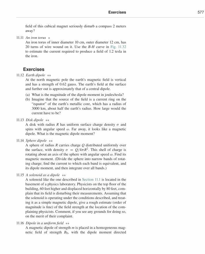
Exercises 577
field of this cubical magnet seriously disturb a compass 2 metersaway?
11.11 An iron torus *An iron torus of inner diameter 10 cm, outer diameter 12 cm, has20 turns of wire wound on it. Use the B-H curve in Fig. 11.32to estimate the current required to produce a field of 1.2 tesla inthe iron.
Exercises11.12 Earth dipole **
At the north magnetic pole the earth’s magnetic field is verticaland has a strength of 0.62 gauss. The earth’s field at the surfaceand further out is approximately that of a central dipole.
(a) What is the magnitude of the dipole moment in joules/tesla?(b) Imagine that the source of the field is a current ring on the
“equator” of the earth’s metallic core, which has a radius of3000 km, about half the earth’s radius. How large would thecurrent have to be?
11.13 Disk dipole **A disk with radius R has uniform surface charge density σ andspins with angular speed ω. Far away, it looks like a magneticdipole. What is the magnetic dipole moment?
11.14 Sphere dipole **A sphere of radius R carries charge Q distributed uniformly overthe surface, with density σ = Q/4πR2. This shell of charge isrotating about an axis of the sphere with angular speed ω. Find itsmagnetic moment. (Divide the sphere into narrow bands of rotat-ing charge; find the current to which each band is equivalent, andits dipole moment, and then integrate over all bands.)
11.15 A solenoid as a dipole **A solenoid like the one described in Section 11.1 is located in thebasement of a physics laboratory. Physicists on the top floor of thebuilding, 60 feet higher and displaced horizontally by 80 feet, com-plain that its field is disturbing their measurements. Assuming thatthe solenoid is operating under the conditions described, and treat-ing it as a simple magnetic dipole, give a rough estimate (order ofmagnitude is fine) of the field strength at the location of the com-plaining physicists. Comment, if you see any grounds for doing so,on the merit of their complaint.
11.16 Dipole in a uniform field **A magnetic dipole of strength m is placed in a homogeneous mag-netic field of strength B0, with the dipole moment directed
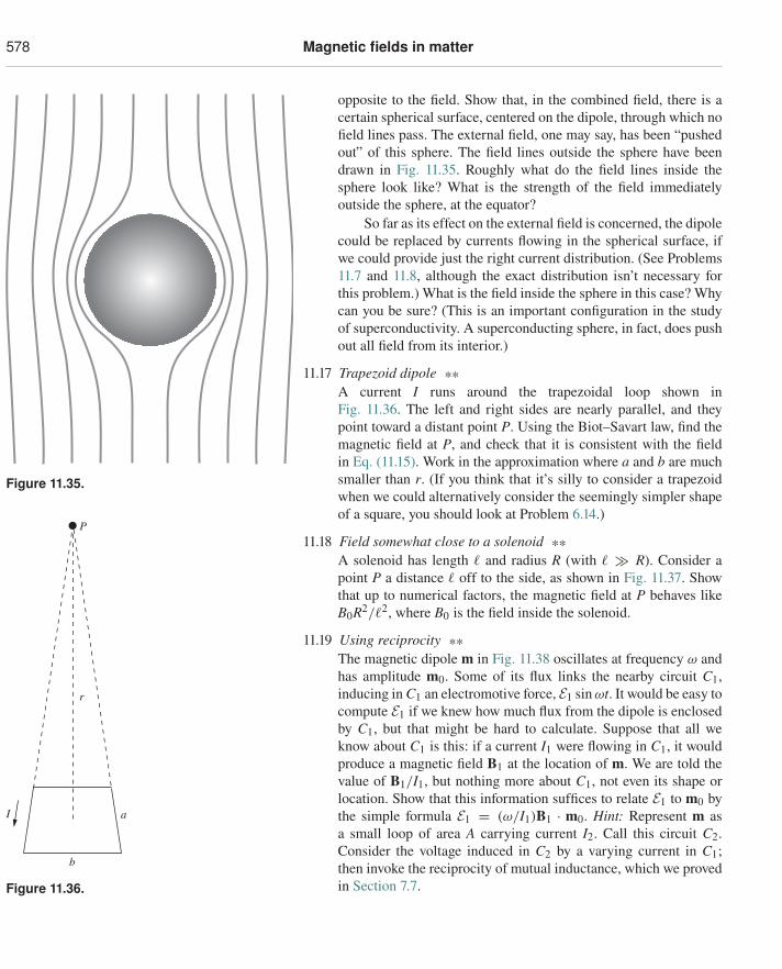
578 Magnetic fields in matter
opposite to the field. Show that, in the combined field, there is acertain spherical surface, centered on the dipole, through which nofield lines pass. The external field, one may say, has been “pushedout” of this sphere. The field lines outside the sphere have beendrawn in Fig. 11.35. Roughly what do the field lines inside thesphere look like? What is the strength of the field immediatelyoutside the sphere, at the equator?
Figure 11.35.
So far as its effect on the external field is concerned, the dipolecould be replaced by currents flowing in the spherical surface, ifwe could provide just the right current distribution. (See Problems11.7 and 11.8, although the exact distribution isn’t necessary forthis problem.) What is the field inside the sphere in this case? Whycan you be sure? (This is an important configuration in the studyof superconductivity. A superconducting sphere, in fact, does pushout all field from its interior.)
11.17 Trapezoid dipole **A current I runs around the trapezoidal loop shown inFig. 11.36. The left and right sides are nearly parallel, and theypoint toward a distant point P. Using the Biot–Savart law, find themagnetic field at P, and check that it is consistent with the fieldin Eq. (11.15). Work in the approximation where a and b are muchsmaller than r. (If you think that it’s silly to consider a trapezoidwhen we could alternatively consider the seemingly simpler shapeof a square, you should look at Problem 6.14.)
11.18 Field somewhat close to a solenoid **A solenoid has length � and radius R (with � � R). Consider apoint P a distance � off to the side, as shown in Fig. 11.37. Showthat up to numerical factors, the magnetic field at P behaves likeB0R2/�2, where B0 is the field inside the solenoid.
a
b
r
P
I
Figure 11.36.
11.19 Using reciprocity **The magnetic dipole m in Fig. 11.38 oscillates at frequency ω andhas amplitude m0. Some of its flux links the nearby circuit C1,inducing in C1 an electromotive force, E1 sin ωt. It would be easy tocompute E1 if we knew how much flux from the dipole is enclosedby C1, but that might be hard to calculate. Suppose that all weknow about C1 is this: if a current I1 were flowing in C1, it wouldproduce a magnetic field B1 at the location of m. We are told thevalue of B1/I1, but nothing more about C1, not even its shape orlocation. Show that this information suffices to relate E1 to m0 bythe simple formula E1 = (ω/I1)B1 · m0. Hint: Represent m asa small loop of area A carrying current I2. Call this circuit C2.Consider the voltage induced in C2 by a varying current in C1;then invoke the reciprocity of mutual inductance, which we provedin Section 7.7.
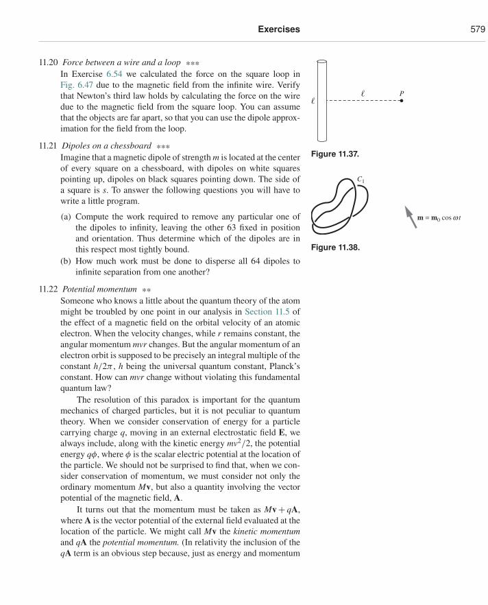
Exercises 579
11.20 Force between a wire and a loop ***In Exercise 6.54 we calculated the force on the square loop inFig. 6.47 due to the magnetic field from the infinite wire. Verifythat Newton’s third law holds by calculating the force on the wiredue to the magnetic field from the square loop. You can assumethat the objects are far apart, so that you can use the dipole approx-imation for the field from the loop.
P
Figure 11.37.
m = m0 cos w t
C1
Figure 11.38.
11.21 Dipoles on a chessboard ***Imagine that a magnetic dipole of strength m is located at the centerof every square on a chessboard, with dipoles on white squarespointing up, dipoles on black squares pointing down. The side ofa square is s. To answer the following questions you will have towrite a little program.
(a) Compute the work required to remove any particular one ofthe dipoles to infinity, leaving the other 63 fixed in positionand orientation. Thus determine which of the dipoles are inthis respect most tightly bound.
(b) How much work must be done to disperse all 64 dipoles toinfinite separation from one another?
11.22 Potential momentum **Someone who knows a little about the quantum theory of the atommight be troubled by one point in our analysis in Section 11.5 ofthe effect of a magnetic field on the orbital velocity of an atomicelectron. When the velocity changes, while r remains constant, theangular momentum mvr changes. But the angular momentum of anelectron orbit is supposed to be precisely an integral multiple of theconstant h/2π , h being the universal quantum constant, Planck’sconstant. How can mvr change without violating this fundamentalquantum law?
The resolution of this paradox is important for the quantummechanics of charged particles, but it is not peculiar to quantumtheory. When we consider conservation of energy for a particlecarrying charge q, moving in an external electrostatic field E, wealways include, along with the kinetic energy mv2/2, the potentialenergy qφ, where φ is the scalar electric potential at the location ofthe particle. We should not be surprised to find that, when we con-sider conservation of momentum, we must consider not only theordinary momentum Mv, but also a quantity involving the vectorpotential of the magnetic field, A.
It turns out that the momentum must be taken as Mv+ qA,where A is the vector potential of the external field evaluated at thelocation of the particle. We might call Mv the kinetic momentumand qA the potential momentum. (In relativity the inclusion of theqA term is an obvious step because, just as energy and momentum
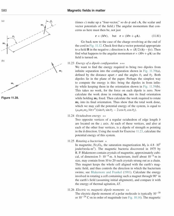
580 Magnetic fields in matter
(times c) make up a “four-vector,” so do φ and cA, the scalar andvector potentials of the field.) The angular momentum that con-cerns us here must then be, not just
r × (Mv), but r × (Mv + qA). (11.81)
(a)
r
m2
m1
q2
q1
(b)
m1
m2
Figure 11.39.
Go back now to the case of the charge revolving at the end ofthe cord in Fig. 11.12. Check first that a vector potential appropriateto a field B in the negative z direction is A = (B/2)(xy− yx). Thenfind what happens to the angular momentum r× (Mv+qA) as thefield is turned on.
11.23 Energy of a dipole configuration ***We want to find the energy required to bring two dipoles frominfinite separation into the configuration shown in Fig. 11.39(a),defined by the distance apart r and the angles θ1 and θ2. Bothdipoles lie in the plane of the paper. Perhaps the simplest wayto compute the energy is this: bring the dipoles in from infin-ity while keeping them in the orientation shown in Fig. 11.39(b).This takes no work, for the force on each dipole is zero. Nowcalculate the work done in rotating m1 into its final orientationwhile holding m2 fixed. Then calculate the work required to rotatem2 into its final orientation. Thus show that the total work done,which we may call the potential energy of the system, is equal to(μ0m1m2/4πr3)(sin θ1 sin θ2 − 2 cos θ1 cos θ2).
11.24 Octahedron energy **Two opposite vertices of a regular octahedron of edge length bare located on the z axis. At each of these vertices, and also ateach of the other four vertices, is a dipole of strength m pointingin the z direction. Using the result for Exercise 11.23, calculate thepotential energy of this system.
11.25 Rotating a bacterium *In magnetite, Fe3O4, the saturation magnetization M0 is 4.8 · 105
joule/(tesla-m3). The magnetic bacteria discovered in 1975 byR. P. Blakemore contain crystals of magnetite, approximately cubi-cal, of dimension 5 · 10−8 m. A bacterium, itself about 10−6 m insize, may contain from 10 to 20 such crystals strung out as a chain.This magnet keeps the whole cell aligned with the earth’s mag-netic field, and thus controls the direction in which the bacteriumswims; see Blakemore and Frankel (1981). Calculate the energyinvolved in rotating a cell containing such a magnet through 90◦ inthe earth’s field (assuming initial alignment), and compare it withthe energy of thermal agitation, kT .
11.26 Electric vs. magnetic dipole moments **The electric dipole moment of a polar molecule is typically 10−30
or 10−29 C-m in order of magnitude (see Fig. 10.14). The magnetic
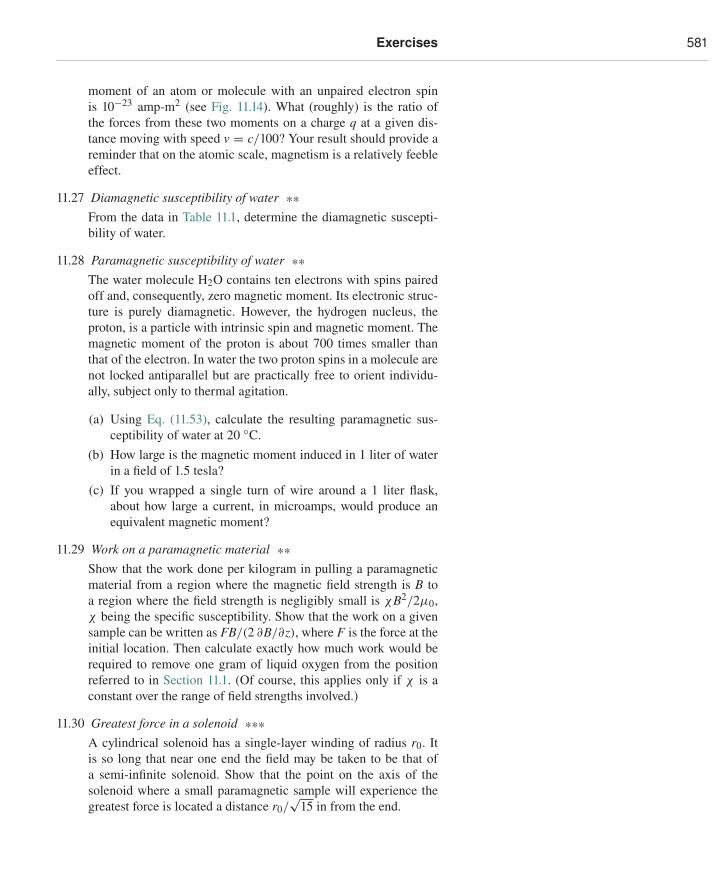
Exercises 581
moment of an atom or molecule with an unpaired electron spinis 10−23 amp-m2 (see Fig. 11.14). What (roughly) is the ratio ofthe forces from these two moments on a charge q at a given dis-tance moving with speed v = c/100? Your result should provide areminder that on the atomic scale, magnetism is a relatively feebleeffect.
11.27 Diamagnetic susceptibility of water **From the data in Table 11.1, determine the diamagnetic suscepti-bility of water.
11.28 Paramagnetic susceptibility of water **The water molecule H2O contains ten electrons with spins pairedoff and, consequently, zero magnetic moment. Its electronic struc-ture is purely diamagnetic. However, the hydrogen nucleus, theproton, is a particle with intrinsic spin and magnetic moment. Themagnetic moment of the proton is about 700 times smaller thanthat of the electron. In water the two proton spins in a molecule arenot locked antiparallel but are practically free to orient individu-ally, subject only to thermal agitation.
(a) Using Eq. (11.53), calculate the resulting paramagnetic sus-ceptibility of water at 20 ◦C.
(b) How large is the magnetic moment induced in 1 liter of waterin a field of 1.5 tesla?
(c) If you wrapped a single turn of wire around a 1 liter flask,about how large a current, in microamps, would produce anequivalent magnetic moment?
11.29 Work on a paramagnetic material **Show that the work done per kilogram in pulling a paramagneticmaterial from a region where the magnetic field strength is B toa region where the field strength is negligibly small is χB2/2μ0,χ being the specific susceptibility. Show that the work on a givensample can be written as FB/(2 ∂B/∂z), where F is the force at theinitial location. Then calculate exactly how much work would berequired to remove one gram of liquid oxygen from the positionreferred to in Section 11.1. (Of course, this applies only if χ is aconstant over the range of field strengths involved.)
11.30 Greatest force in a solenoid ***A cylindrical solenoid has a single-layer winding of radius r0. Itis so long that near one end the field may be taken to be that ofa semi-infinite solenoid. Show that the point on the axis of thesolenoid where a small paramagnetic sample will experience thegreatest force is located a distance r0/
√15 in from the end.
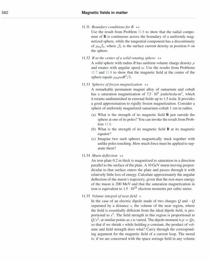
582 Magnetic fields in matter
11.31 Boundary conditions for B **Use the result from Problem 11.8 to show that the radial compo-nent of B is continuous across the boundary of a uniformly mag-netized sphere, while the tangential component has a discontinuityof μ0Jθ , where Jθ is the surface current density at position θ onthe sphere.
11.32 B at the center of a solid rotating sphere **A solid sphere with radius R has uniform volume charge density ρ
and rotates with angular speed ω. Use the results from Problems11.7 and 11.8 to show that the magnetic field at the center of thesphere equals μ0ρωR2/3.
11.33 Spheres of frozen magnetization **A remarkable permanent magnet alloy of samarium and cobalthas a saturation magnetization of 7.5 · 105 joule/tesla-m3, whichit retains undiminished in external fields up to 1.5 tesla. It providesa good approximation to rigidly frozen magnetization. Consider asphere of uniformly magnetized samarium-cobalt 1 cm in radius.
(a) What is the strength of its magnetic field B just outside thesphere at one of its poles? You can invoke the result from Prob-lem 11.8.
(b) What is the strength of its magnetic field B at its magneticequator?
(c) Imagine two such spheres magnetically stuck together withunlike poles touching. How much force must be applied to sep-arate them?
11.34 Muon deflection **An iron plate 0.2 m thick is magnetized to saturation in a directionparallel to the surface of the plate. A 10 GeV muon moving perpen-dicular to that surface enters the plate and passes through it withrelatively little loss of energy. Calculate approximately the angulardeflection of the muon’s trajectory, given that the rest-mass energyof the muon is 200 MeV and that the saturation magnetization iniron is equivalent to 1.5 · 1029 electron moments per cubic meter.
11.35 Volume integral of near field *In the case of an electric dipole made of two charges Q and −Qseparated by a distance s, the volume of the near region, wherethe field is essentially different from the ideal dipole field, is pro-portional to s3. The field strength in this region is proportional toQ/s2, at similar points as s is varied. The dipole moment is p = Qs,so that if we shrink s while holding p constant, the product of vol-ume and field strength does what? Carry through the correspond-ing argument for the magnetic field of a current loop. The moralis: if we are concerned with the space average field in any volume
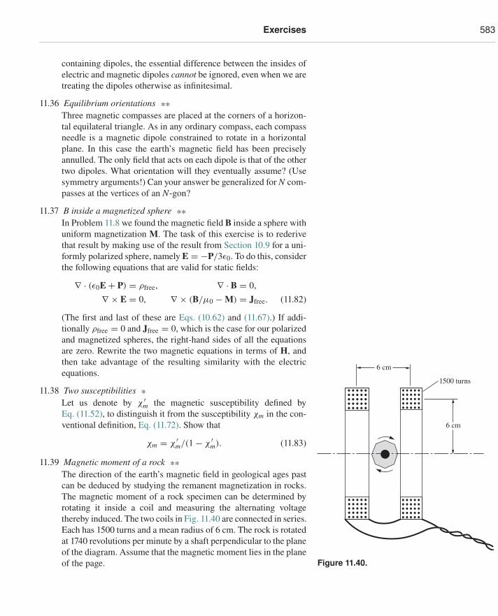
Exercises 583
containing dipoles, the essential difference between the insides ofelectric and magnetic dipoles cannot be ignored, even when we aretreating the dipoles otherwise as infinitesimal.
11.36 Equilibrium orientations **Three magnetic compasses are placed at the corners of a horizon-tal equilateral triangle. As in any ordinary compass, each compassneedle is a magnetic dipole constrained to rotate in a horizontalplane. In this case the earth’s magnetic field has been preciselyannulled. The only field that acts on each dipole is that of the othertwo dipoles. What orientation will they eventually assume? (Usesymmetry arguments!) Can your answer be generalized for N com-passes at the vertices of an N-gon?
11.37 B inside a magnetized sphere **In Problem 11.8 we found the magnetic field B inside a sphere withuniform magnetization M. The task of this exercise is to rederivethat result by making use of the result from Section 10.9 for a uni-formly polarized sphere, namely E = −P/3ε0. To do this, considerthe following equations that are valid for static fields:
∇ · (ε0E + P) = ρfree, ∇ · B = 0,∇ × E = 0, ∇ × (B/μ0 − M) = Jfree. (11.82)
(The first and last of these are Eqs. (10.62) and (11.67).) If addi-tionally ρfree = 0 and Jfree = 0, which is the case for our polarizedand magnetized spheres, the right-hand sides of all the equationsare zero. Rewrite the two magnetic equations in terms of H, andthen take advantage of the resulting similarity with the electricequations.
6 cm
6 cm
1500 turns
Figure 11.40.
11.38 Two susceptibilities *Let us denote by χ ′
m the magnetic susceptibility defined byEq. (11.52), to distinguish it from the susceptibility χm in the con-ventional definition, Eq. (11.72). Show that
χm = χ ′m/(1 − χ ′
m). (11.83)
11.39 Magnetic moment of a rock **The direction of the earth’s magnetic field in geological ages pastcan be deduced by studying the remanent magnetization in rocks.The magnetic moment of a rock specimen can be determined byrotating it inside a coil and measuring the alternating voltagethereby induced. The two coils in Fig. 11.40 are connected in series.Each has 1500 turns and a mean radius of 6 cm. The rock is rotatedat 1740 revolutions per minute by a shaft perpendicular to the planeof the diagram. Assume that the magnetic moment lies in the planeof the page.
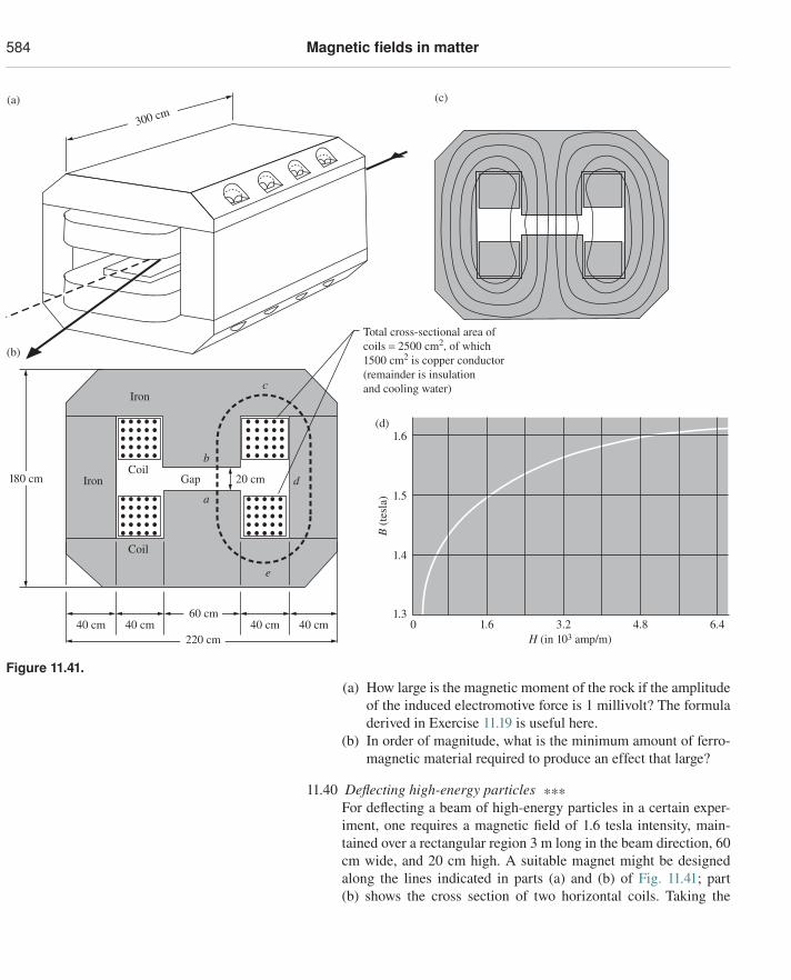
584 Magnetic fields in matter
01.3
220 cm40 cm40 cm40 cm40 cm
60 cm
300 cm
20 cm d
c
b
a
e
Total cross-sectional area ofcoils = 2500 cm2, of which1500 cm2 is copper conductor(remainder is insulationand cooling water)
180 cm Iron
(a)
(b)
(c)
(d)
Iron
Coil
CoilGap
1.4
1.5
1.6
1.6
B (t
esla
)
H (in 103 amp/m)3.2 4.8 6.4
Figure 11.41.(a) How large is the magnetic moment of the rock if the amplitude
of the induced electromotive force is 1 millivolt? The formuladerived in Exercise 11.19 is useful here.
(b) In order of magnitude, what is the minimum amount of ferro-magnetic material required to produce an effect that large?
11.40 Deflecting high-energy particles ***For deflecting a beam of high-energy particles in a certain exper-iment, one requires a magnetic field of 1.6 tesla intensity, main-tained over a rectangular region 3 m long in the beam direction, 60cm wide, and 20 cm high. A suitable magnet might be designedalong the lines indicated in parts (a) and (b) of Fig. 11.41; part(b) shows the cross section of two horizontal coils. Taking the
Exercises 585
dimensions as given (you can make rough estimates for any otherlengths you need), and referring to the additional comments below,determine:
(a) the total number of ampere turns required in the two coils toproduce a 1.6 tesla field in the gap;
(b) the power in kilowatts that must be supplied;(c) the number of turns that each coil should contain, and the cor-
responding cross-sectional area of the wire, so that the desiredfield will be attained when the coils are connected in series toa 400 volt dc power supply.
For use in (a), a portion of the B-H curve for Armco magnetiron is shown in Fig. 11.41(d). All that you need to determine isthe line integral of H around a path like abcdea. In the gap, H =B/μ0. In the iron, you may assume that B has the same intensityas in the gap. The field lines will look something like those inFig. 11.41(c). You can estimate roughly the length of path in theiron. This is not very critical, for you will find that the long pathbcdea contributes a relatively small amount to the line integral,compared with the contribution of the air path ab. In fact, it isnot a bad approximation, at lower field strengths, to neglect H inthe iron.
For (b), let each coil contain N turns, and assume the resistiv-ity of copper is ρ = 2.0 · 10−8 ohm-m. You will find that the powerrequired for a given number of ampere turns is independent of N;that is, it is the same for many turns of fine wire or a few turns ofthick wire, provided that the total cross section of copper is fixedas specified (1500 cm2 in our setup). The designer therefore selectsN and conductor cross section to match the magnet to the voltageof the intended power source.
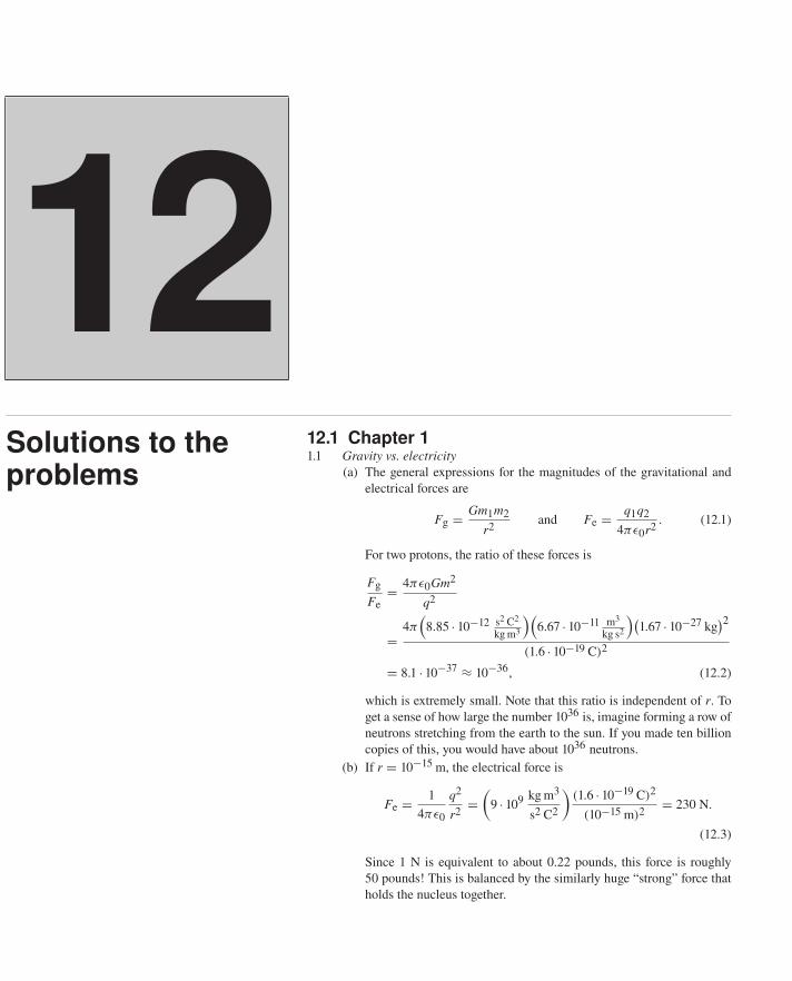
12Solutions to theproblems
12.1 Chapter 11.1 Gravity vs. electricity
(a) The general expressions for the magnitudes of the gravitational andelectrical forces are
Fg = Gm1m2r2 and Fe = q1q2
4πε0r2 . (12.1)
For two protons, the ratio of these forces is
Fg
Fe= 4πε0Gm2
q2
=4π
(8.85 · 10−12 s2 C2
kg m3
)(6.67 · 10−11 m3
kg s2
)(1.67 · 10−27 kg
)2
(1.6 · 10−19 C)2
= 8.1 · 10−37 ≈ 10−36, (12.2)
which is extremely small. Note that this ratio is independent of r. Toget a sense of how large the number 1036 is, imagine forming a row ofneutrons stretching from the earth to the sun. If you made ten billioncopies of this, you would have about 1036 neutrons.
(b) If r = 10−15 m, the electrical force is
Fe = 14πε0
q2
r2 =(
9 · 109 kg m3
s2 C2
)(1.6 · 10−19 C)2
(10−15 m)2 = 230 N.
(12.3)
Since 1 N is equivalent to about 0.22 pounds, this force is roughly50 pounds! This is balanced by the similarly huge “strong” force thatholds the nucleus together.
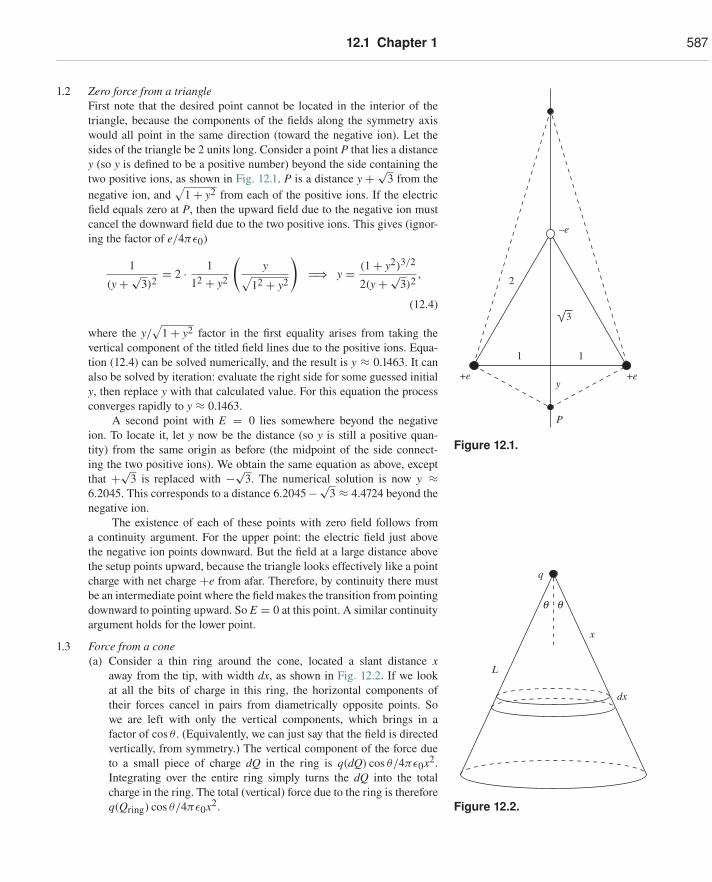
12.1 Chapter 1 587
1.2 Zero force from a triangleFirst note that the desired point cannot be located in the interior of thetriangle, because the components of the fields along the symmetry axis
–e
+e +e
1 1
2
3
y
P
Figure 12.1.
would all point in the same direction (toward the negative ion). Let thesides of the triangle be 2 units long. Consider a point P that lies a distancey (so y is defined to be a positive number) beyond the side containing thetwo positive ions, as shown in Fig. 12.1. P is a distance y + √
3 from thenegative ion, and
√1 + y2 from each of the positive ions. If the electric
field equals zero at P, then the upward field due to the negative ion mustcancel the downward field due to the two positive ions. This gives (ignor-ing the factor of e/4πε0)
1
(y +√3)2
= 2 · 112 + y2
(y√
12 + y2
)�⇒ y = (1 + y2)3/2
2(y +√3)2
,
(12.4)
where the y/√
1 + y2 factor in the first equality arises from taking thevertical component of the titled field lines due to the positive ions. Equa-tion (12.4) can be solved numerically, and the result is y ≈ 0.1463. It canalso be solved by iteration: evaluate the right side for some guessed initialy, then replace y with that calculated value. For this equation the processconverges rapidly to y ≈ 0.1463.
A second point with E = 0 lies somewhere beyond the negativeion. To locate it, let y now be the distance (so y is still a positive quan-tity) from the same origin as before (the midpoint of the side connect-ing the two positive ions). We obtain the same equation as above, exceptthat +√3 is replaced with −√3. The numerical solution is now y ≈6.2045. This corresponds to a distance 6.2045−√
3 ≈ 4.4724 beyond thenegative ion.
The existence of each of these points with zero field follows froma continuity argument. For the upper point: the electric field just abovethe negative ion points downward. But the field at a large distance abovethe setup points upward, because the triangle looks effectively like a pointcharge with net charge +e from afar. Therefore, by continuity there mustbe an intermediate point where the field makes the transition from pointing
q
x
dx
L
Figure 12.2.
downward to pointing upward. So E = 0 at this point. A similar continuityargument holds for the lower point.
1.3 Force from a cone(a) Consider a thin ring around the cone, located a slant distance x
away from the tip, with width dx, as shown in Fig. 12.2. If we lookat all the bits of charge in this ring, the horizontal components oftheir forces cancel in pairs from diametrically opposite points. Sowe are left with only the vertical components, which brings in afactor of cos θ . (Equivalently, we can just say that the field is directedvertically, from symmetry.) The vertical component of the force dueto a small piece of charge dQ in the ring is q(dQ) cos θ/4πε0x2.Integrating over the entire ring simply turns the dQ into the totalcharge in the ring. The total (vertical) force due to the ring is thereforeq(Qring) cos θ/4πε0x2.
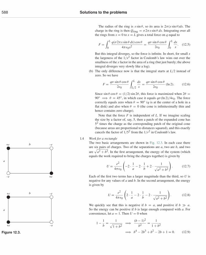
588 Solutions to the problems
The radius of the ring is x sin θ , so its area is 2π(x sin θ)dx. Thecharge in the ring is then Qring = σ2πx sin θ dx. Integrating over allthe rings from x = 0 to x = L gives a total force on q equal to
F =∫ L
0
q(σ2πx sin θ dx) cos θ
4πε0x2 = qσ sin θ cos θ
2ε0
∫ L
0
dxx
. (12.5)
But this integral diverges, so the force is infinite. In short, for small xthe largeness of the 1/x2 factor in Coulomb’s law wins out over thesmallness of the x factor in the area of a ring (but just barely; the aboveintegral diverges very slowly like a log).
(b) The only difference now is that the integral starts at L/2 instead ofzero. So we have
F = qσ sin θ cos θ
2ε0
∫ L
L/2
dxx
= qσ sin θ cos θ
2ε0(ln 2). (12.6)
Since sin θ cos θ = (1/2) sin 2θ , this force is maximized when 2θ =90◦ �⇒ θ = 45◦, in which case it equals qσ(ln 2)/4ε0. The forcecorrectly equals zero when θ = 90◦ (q is at the center of a hole in aflat disk) and also when θ = 0 (the cone is infinitesimally thin andhence contains zero charge).
Note that the force F is independent of L. If we imagine scalingthe size by a factor of, say, 5, then a patch of the expanded cone has52 times the charge as the corresponding patch of the original cone(because areas are proportional to distances squared), and this exactlycancels the factor of 1/52 from the 1/r2 in Coulomb’s law.
1.4 Work for a rectangleThe two basic arrangements are shown in Fig. 12.3. In each case there–e+e
+e–e
b
a
–e+e
–e+e
b
a
Figure 12.3.
are six pairs of charges. Two of the separations are a, two are b, and twoare
√a2 + b2. In the first arrangement, the energy of the system (which
equals the work required to bring the charges together) is given by
U = e2
4πε0
(−2 · 1
a− 2 · 1
b+ 2 · 1√
a2 + b2
). (12.7)
Each of the first two terms has a larger magnitude than the third, so U isnegative for any values of a and b. In the second arrangement, the energyis given by
U = e2
4πε0
(2 · 1
a− 2 · 1
b− 2 · 1√
a2 + b2
). (12.8)
We quickly see that this is negative if b = a, and positive if b � a.So the energy can be positive if b is large enough compared with a. Forconvenience, let a = 1. Then U = 0 when
1 − 1b= 1√
1 + b2�⇒ (b − 1)2
b2 = 11 + b2
�⇒ b4 − 2b3 + b2 − 2b + 1 = 0. (12.9)
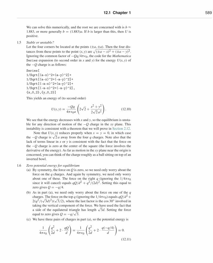
12.1 Chapter 1 589
We can solve this numerically, and the root we are concerned with is b ≈1.883, or more generally b = (1.883)a. If b is larger than this, then U ispositive.
1.5 Stable or unstable?Let the four corners be located at the points (±a,±a). Then the four dis-tances from these points to the point (x, y) are
√(±a − x)2 + (±a − y)2.
Ignoring the common factor of −Qq/4πε0, the code for the MathematicaSeries expansion (to second order in x and y) for the energy U(x, y) ofthe −Q charge is as follows:
Series[1/Sqrt[(a-x)^2+(a-y)^2]+1/Sqrt[(a-x)^2+(-a-y)^2]+1/Sqrt[(-a-x)^2+(a-y)^2]+1/Sqrt[(-a-x)^2+(-a-y)^2],{x,0,2},{y,0,2}]
This yields an energy of (to second order)
U(x, y) = −Qq4πε0a
(2√
2 + x2 + y2
2√
2 a2
). (12.10)
We see that the energy decreases with x and y, so the equilibrium is unsta-ble for any direction of motion of the −Q charge in the xy plane. Thisinstability is consistent with a theorem that we will prove in Section 2.12.
Note that U(x, y) reduces properly when x = y = 0, in which casethe −Q charge is
√2 a away from the four q charges. Note also that the
lack of terms linear in x or y is consistent with the fact that the force onthe −Q charge is zero at the center of the square (the force involves thederivative of the energy). As far as motion in the xy plane near the origin isconcerned, you can think of the charge roughly as a ball sitting on top of aninverted bowl.
1.6 Zero potential energy for equilibrium(a) By symmetry, the force on Q is zero, so we need only worry about the
force on the q charges. And again by symmetry, we need only worryabout one of these. The force on the right q (ignoring the 1/4πε0since it will cancel) equals qQ/d2 + q2/(2d)2. Setting this equal tozero gives Q = −q/4.
(b) As in part (a), we need only worry about the force on one of the qcharges. The force on the top q (ignoring the 1/4πε0) equals qQ/d2+2(q2/(
√3d)2)(
√3/2), where the last factor is the cos 30◦ involved in
taking the vertical component of the force. We have used the fact thata side of the equilateral triangle has length
√3d. Setting the force
equal to zero gives Q = −q/√
3.(c) We have three pairs of charges in part (a), so the potential energy is
14πε0
(q2
2d+ 2 · qQ
d
)= 1
4πε0
(q2
2d+ 2 · q(−q/4)
d
)= 0.
(12.11)
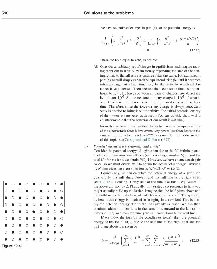
590 Solutions to the problems
We have six pairs of charges in part (b), so the potential energy is
14πε0
(3 · q2
√3d
+ 3 · qQd
)= 1
4πε0
(3 · q2
√3d
+ 3 · q(−q/√
3)
d
)
= 0. (12.12)
These are both equal to zero, as desired.
(d) Consider an arbitrary set of charges in equilibrium, and imagine mov-ing them out to infinity by uniformly expanding the size of the con-figuration, so that all relative distances stay the same. For example, inpart (b) we will simply expand the equilateral triangle until it becomesinfinitely large. At a later time, let f be the factor by which all dis-tances have increased. Then because the electrostatic force is propor-tional to 1/r2, the forces between all pairs of charges have decreasedby a factor 1/f 2. So the net force on any charge is 1/f 2 of what itwas at the start. But it was zero at the start, so it is zero at any latertime. Therefore, since the force on any charge is always zero, zerowork is needed to bring it out to infinity. The initial potential energyof the system is thus zero, as desired. (You can quickly show with acounterexample that the converse of our result is not true.)
From this reasoning, we see that the particular inverse-square natureof the electrostatic force is irrelevant. Any power-law force leads to thesame result. But a force such as e−αr does not. For further discussionof this topic, see Crosignani and Di Porto (1977).
1.7 Potential energy in a two-dimensional crystalConsider the potential energy of a given ion due to the full infinite plane.Call it U0. If we sum over all ions (or a very large number N) to find thetotal U of these ions, we obtain NU0. However, we have counted each pair
Figure 12.4.
twice, so we must divide by 2 to obtain the actual total energy. Dividingby N then gives the energy per ion as (NU0/2)/N = U0/2.
Equivalently, we can calculate the potential energy of a given iondue to only the half-plane above it and the half-line to the right of it;see Fig. 12.4. Looking at only half of the ions like this is equivalent tothe above division by 2. Physically, this strategy corresponds to how youmight actually build up the lattice. Imagine that the half-plane above andthe half-line to the right have already been put in position. The questionis, how much energy is involved in bringing in a new ion? This is sim-ply the potential energy due to the ions already in place. We can thencontinue adding on new ions in the same line, onward to the left (as inExercise 1.42), and then eventually we can move down to the next line.
If we index the ions by the coordinates (m, n), then the potentialenergy of the ion at (0, 0) due to the half-line to the right of it and thehalf-plane above it is given by
U = e2
4πε0a
⎛⎝ ∞∑
m=1
(−1)m
m+
∞∑n=1
∞∑m=−∞
(−1)m+n√m2 + n2
⎞⎠ . (12.13)
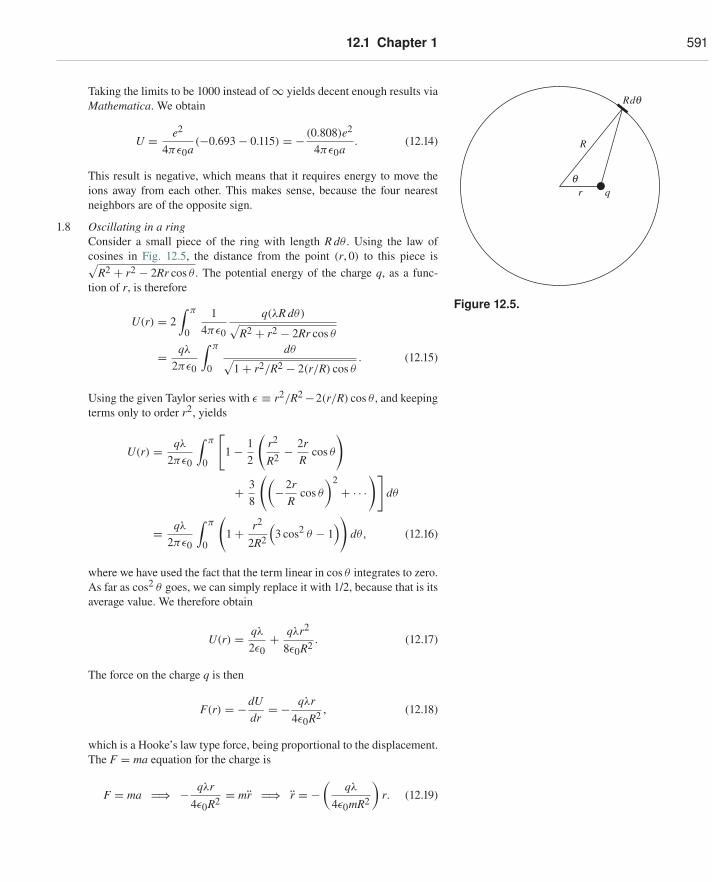
12.1 Chapter 1 591
Taking the limits to be 1000 instead of ∞ yields decent enough results viaMathematica. We obtain
U = e2
4πε0a(−0.693 − 0.115) = − (0.808)e2
4πε0a. (12.14)
This result is negative, which means that it requires energy to move theions away from each other. This makes sense, because the four nearestneighbors are of the opposite sign.
1.8 Oscillating in a ringConsider a small piece of the ring with length R dθ . Using the law ofcosines in Fig. 12.5, the distance from the point (r, 0) to this piece is
q
R
q
R dq
r
Figure 12.5.
√R2 + r2 − 2Rr cos θ . The potential energy of the charge q, as a func-
tion of r, is therefore
U(r) = 2∫ π
0
14πε0
q(λR dθ)√R2 + r2 − 2Rr cos θ
= qλ
2πε0
∫ π
0
dθ√1 + r2/R2 − 2(r/R) cos θ
. (12.15)
Using the given Taylor series with ε ≡ r2/R2 −2(r/R) cos θ , and keepingterms only to order r2, yields
U(r) = qλ
2πε0
∫ π
0
[1 − 1
2
(r2
R2 − 2rR
cos θ
)
+ 38
((−2r
Rcos θ
)2+ · · ·
)]dθ
= qλ
2πε0
∫ π
0
(1 + r2
2R2
(3 cos2 θ − 1
))dθ , (12.16)
where we have used the fact that the term linear in cos θ integrates to zero.As far as cos2 θ goes, we can simply replace it with 1/2, because that is itsaverage value. We therefore obtain
U(r) = qλ
2ε0+ qλr2
8ε0R2 . (12.17)
The force on the charge q is then
F(r) = −dUdr
= − qλr4ε0R2 , (12.18)
which is a Hooke’s law type force, being proportional to the displacement.The F = ma equation for the charge is
F = ma �⇒ − qλr4ε0R2 = mr �⇒ r = −
(qλ
4ε0mR2
)r. (12.19)
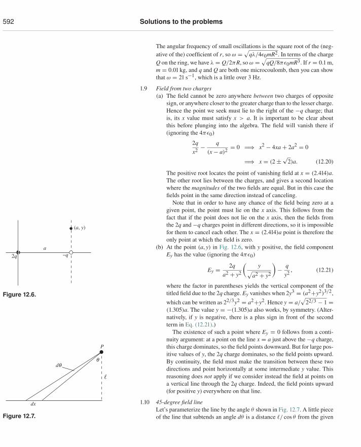
592 Solutions to the problems
The angular frequency of small oscillations is the square root of the (neg-ative of the) coefficient of r, so ω =
√qλ/4ε0mR2. In terms of the charge
Q on the ring, we have λ = Q/2πR, so ω =√
qQ/8πε0mR3. If r = 0.1 m,m = 0.01 kg, and q and Q are both one microcoulomb, then you can showthat ω = 21 s−1, which is a little over 3 Hz.
1.9 Field from two charges(a) The field cannot be zero anywhere between two charges of opposite
sign, or anywhere closer to the greater charge than to the lesser charge.Hence the point we seek must lie to the right of the −q charge; thatis, its x value must satisfy x > a. It is important to be clear aboutthis before plunging into the algebra. The field will vanish there if(ignoring the 4πε0)
2qx2 − q
(x − a)2 = 0 �⇒ x2 − 4xa + 2a2 = 0
�⇒ x = (2 ±√2)a. (12.20)
The positive root locates the point of vanishing field at x = (2.414)a.The other root lies between the charges, and gives a second locationwhere the magnitudes of the two fields are equal. But in this case thefields point in the same direction instead of canceling.
Note that in order to have any chance of the field being zero at agiven point, the point must lie on the x axis. This follows from thefact that if the point does not lie on the x axis, then the fields fromthe 2q and −q charges point in different directions, so it is impossiblefor them to cancel each other. The x = (2.414)a point is therefore theonly point at which the field is zero.
(b) At the point (a, y) in Fig. 12.6, with y positive, the field component2q –q
a
(a, y)
Figure 12.6.
Ey has the value (ignoring the 4πε0)
Ey = 2qa2 + y2
(y√
a2 + y2
)− q
y2 , (12.21)
where the factor in parentheses yields the vertical component of thetitled field due to the 2q charge. Ey vanishes when 2y3 = (a2+y2)3/2,
which can be written as 22/3y2 = a2+y2. Hence y = a/√
22/3 − 1 =(1.305)a. The value y = −(1.305)a also works, by symmetry. (Alter-natively, if y is negative, there is a plus sign in front of the secondterm in Eq. (12.21).)
The existence of such a point where Ey = 0 follows from a conti-nuity argument: at a point on the line x = a just above the −q charge,this charge dominates, so the field points downward. But for large pos-itive values of y, the 2q charge dominates, so the field points upward.By continuity, the field must make the transition between these twodirections and point horizontally at some intermediate y value. Thisreasoning does not apply if we consider instead the field at points ona vertical line through the 2q charge. Indeed, the field points upward(for positive y) everywhere on that line.
1.10 45-degree field lineLet’s parameterize the line by the angle θ shown in Fig. 12.7. A little piece
dq
dx
P
q
Figure 12.7. of the line that subtends an angle dθ is a distance �/ cos θ from the given
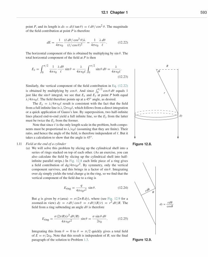
12.1 Chapter 1 593
point P, and its length is dx = d(� tan θ) = � dθ/ cos2 θ . The magnitudeof the field contribution at point P is therefore
dE = 14πε0
(� dθ/ cos2 θ)λ
(�/ cos θ)2 = 14πε0
λ dθ
�. (12.22)
The horizontal component of this is obtained by multiplying by sin θ . Thetotal horizontal component of the field at P is then
Ex =∫ π/2
0
14πε0
λ dθ
�sin θ = λ
4πε0�
∫ π/2
0sin θ dθ = λ
4πε0�.
(12.23)
Similarly, the vertical component of the field contribution in Eq. (12.22)is obtained by multiplying by cos θ . And since
∫ π/20 cos θ dθ equals 1
just like the sin θ integral, we see that Ex and Ey at point P both equalλ/4πε0�. The field therefore points up at a 45◦ angle, as desired.
The Ey = λ/4πε0� result is consistent with the fact that the fieldfrom a full infinite line is λ/2πε0�, which follows from a direct integration
q
r
R
dy
Figure 12.8.
or a quick application of Gauss’s law. By superposition, two half-infinitelines placed end-to-end yield a full infinite line, so the Ey from the lattermust be twice the Ey from the former.
Note that since � is the only length scale in the problem, both compo-nents must be proportional to λ/ε0� (assuming that they are finite). Theirratio, and hence the angle of the field, is therefore independent of �. But ittakes a calculation to show that the angle is 45◦.
1.11 Field at the end of a cylinder(a) We will solve this problem by slicing up the cylindrical shell into a
series of rings stacked on top of each other. (As an exercise, you can
q
dy =
r dq
r dqcosq
Figure 12.9.
also calculate the field by slicing up the cylindrical shell into half-infinite parallel strips.) In Fig. 12.8 each little piece of a ring givesa field contribution of dq/4πε0r2. By symmetry, only the verticalcomponent survives, and this brings in a factor of sin θ . Integratingover dq simply yields the total charge q in the ring, so we find that thevertical component of the field due to a ring is
Ering = q4πε0r2 sin θ . (12.24)
But q is given by σ(area) = σ(2πR dy), where (see Fig. 12.9 for azoomed-in view) dy = r dθ/ cos θ = r dθ/(R/r) = r2 dθ/R. Thefield from a ring subtending an angle dθ is therefore
Ering = σ(2πR)(r2 dθ/R)
4πε0r2 sin θ = σ sin θ dθ
2ε0. (12.25)
Integrating this from θ = 0 to θ = π/2 quickly gives a total fieldof E = σ/2ε0. Note that this result is independent of R; see the finalparagraph of the solution to Problem 1.3.
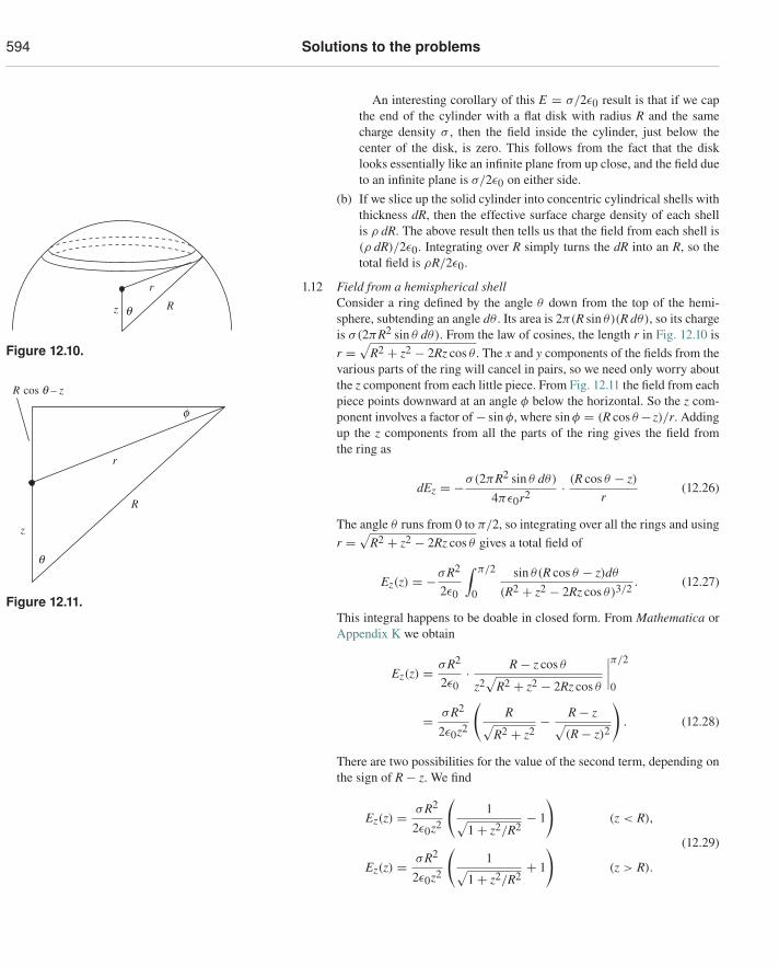
594 Solutions to the problems
An interesting corollary of this E = σ/2ε0 result is that if we capthe end of the cylinder with a flat disk with radius R and the samecharge density σ , then the field inside the cylinder, just below thecenter of the disk, is zero. This follows from the fact that the disklooks essentially like an infinite plane from up close, and the field dueto an infinite plane is σ/2ε0 on either side.
(b) If we slice up the solid cylinder into concentric cylindrical shells withthickness dR, then the effective surface charge density of each shellis ρ dR. The above result then tells us that the field from each shell is(ρ dR)/2ε0. Integrating over R simply turns the dR into an R, so thetotal field is ρR/2ε0.
Rz
r
q
Figure 12.10.
1.12 Field from a hemispherical shellConsider a ring defined by the angle θ down from the top of the hemi-sphere, subtending an angle dθ . Its area is 2π(R sin θ)(R dθ), so its chargeis σ(2πR2 sin θ dθ). From the law of cosines, the length r in Fig. 12.10 isr =
√R2 + z2 − 2Rz cos θ . The x and y components of the fields from the
various parts of the ring will cancel in pairs, so we need only worry aboutthe z component from each little piece. From Fig. 12.11 the field from each
R
R cos q – z
z
r
q
f
Figure 12.11.
piece points downward at an angle φ below the horizontal. So the z com-ponent involves a factor of − sin φ, where sin φ = (R cos θ − z)/r. Addingup the z components from all the parts of the ring gives the field fromthe ring as
dEz = −σ(2πR2 sin θ dθ)
4πε0r2 · (R cos θ − z)r
(12.26)
The angle θ runs from 0 to π/2, so integrating over all the rings and usingr =
√R2 + z2 − 2Rz cos θ gives a total field of
Ez(z) = −σR2
2ε0
∫ π/2
0
sin θ(R cos θ − z)dθ
(R2 + z2 − 2Rz cos θ)3/2 . (12.27)
This integral happens to be doable in closed form. From Mathematica orAppendix K we obtain
Ez(z) = σR2
2ε0· R − z cos θ
z2√
R2 + z2 − 2Rz cos θ
∣∣∣∣π/2
0
= σR2
2ε0z2
(R√
R2 + z2− R − z√
(R − z)2
). (12.28)
There are two possibilities for the value of the second term, depending onthe sign of R − z. We find
Ez(z) = σR2
2ε0z2
(1√
1 + z2/R2− 1
)(z < R),
Ez(z) = σR2
2ε0z2
(1√
1 + z2/R2+ 1
)(z > R).
(12.29)
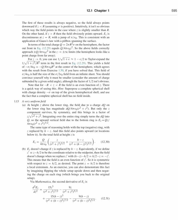
12.1 Chapter 1 595
The first of these results is always negative, so the field always pointsdownward if z < R (assuming σ is positive). Intuitively, it isn’t so obviouswhich way the field points in the case where z is slightly smaller than R.On the other hand, if z > R then the field obviously points upward. Ez isdiscontinuous at z = R, with a jump of σ/ε0. This is consistent with anapplication of Gauss’s law with a pillbox spanning the surface.
In terms of the total charge Q = 2πR2σ on the hemisphere, the factorout front in Eq. (12.29) equals Q/4πε0z2. So the above fields correctlyapproach ±Q/4πε0z2 in the z → ±∞ limits (the hemisphere looks like apoint charge from far away).
For z → 0, you can use 1/√
1 + ε ≈ 1 − ε/2 to Taylor-expand the1/
√1 + z2/R2 term in the first result in Eq. (12.29). This yields a field
of −σ/4ε0 = −Q/8πε0R2 at the center of the hemisphere, which agreeswith the result from Exercise 1.50, if you have solved that. This field ofσ/4ε0 is half the size of the σ/2ε0 field from an infinite sheet. You shouldconvince yourself why it must be smaller (consider the amount of chargesubtended by a given solid angle), although the factor of 1/2 isn’t obvious.
Note that for −R < z < R the field is an even function of z. Thereis a quick way of seeing this. Hint: Superpose a complete spherical shellwith charge density −σ on top of the given hemispherical shell, and usethe fact that a complete spherical shell has no field inside.
1.13 A very uniform field(a) At height z above the lower ring, the field due to a charge dQ on
the lower ring has magnitude dQ/4πε0(r2 + z2). But only the zcomponent survives, by symmetry, and this brings in a factor ofz/
√r2 + z2. Integrating over the entire ring simply turns the dQ into
Q, so the upward vertical field due to the bottom ring is Ez =Qz/4πε0(r2 + z2)3/2.
The same type of reasoning holds with the top (negative) ring, withz replaced by h − z. And this field also points upward (at locationsbelow it). So the total field at height z is
Ez = Q4πε0
(z
(r2 + z2)3/2 + h − z(r2 + (h − z)2)3/2
). (12.30)
(b) Ez doesn’t change if z is replaced by h − z. Equivalently, if we definez′ ≡ z−h/2 to be the coordinate relative to the midpoint, then the fielddoesn’t change when we replace z′ with (h−z)−h/2 = h/2−z = −z′.This means that the field is an even function of z′. So it is symmetricwith respect to z = h/2, as desired. The point z = h/2 is thereforea local extremum. As an exercise, you can also demonstrate this factby imagining flipping the whole setup upside down and then negat-ing the charge on each ring (which brings you back to the originalsetup).
Via Mathematica, the second derivative of Ez is
d2Ez
dz2 = 15z3
(r2 + z2)7/2 − 9z(r2 + z2)5/2
+ 15(h − z)3
(r2 + (h − z)2)7/2 − 9(h − z)(r2 + (h − z)2)5/2 . (12.31)
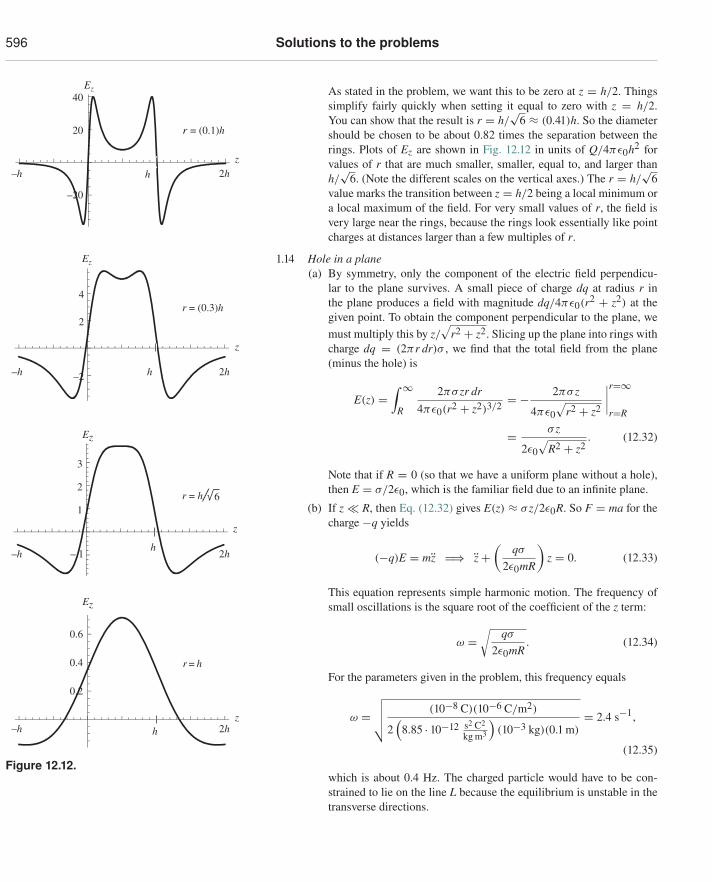
596 Solutions to the problems
As stated in the problem, we want this to be zero at z = h/2. Thingssimplify fairly quickly when setting it equal to zero with z = h/2.You can show that the result is r = h/
√6 ≈ (0.41)h. So the diameter
z
z
z
z
h–h 2h
h–h 2h
–h 2h
h–h 2h
Ez
Ez
Ez
Ez
–2
– 1
–20
2
4
1
2
3
0.2
0.4
0.6
r = h
r = h
r = (0.3)h
r = (0.1)h
6
20
40
h
Figure 12.12.
should be chosen to be about 0.82 times the separation between therings. Plots of Ez are shown in Fig. 12.12 in units of Q/4πε0h2 forvalues of r that are much smaller, smaller, equal to, and larger thanh/√
6. (Note the different scales on the vertical axes.) The r = h/√
6value marks the transition between z = h/2 being a local minimum ora local maximum of the field. For very small values of r, the field isvery large near the rings, because the rings look essentially like pointcharges at distances larger than a few multiples of r.
1.14 Hole in a plane(a) By symmetry, only the component of the electric field perpendicu-
lar to the plane survives. A small piece of charge dq at radius r inthe plane produces a field with magnitude dq/4πε0(r2 + z2) at thegiven point. To obtain the component perpendicular to the plane, wemust multiply this by z/
√r2 + z2. Slicing up the plane into rings with
charge dq = (2πr dr)σ , we find that the total field from the plane(minus the hole) is
E(z) =∫ ∞
R
2πσ zr dr4πε0(r2 + z2)3/2 = − 2πσ z
4πε0√
r2 + z2
∣∣∣∣r=∞r=R
= σ z
2ε0√
R2 + z2. (12.32)
Note that if R = 0 (so that we have a uniform plane without a hole),then E = σ/2ε0, which is the familiar field due to an infinite plane.
(b) If z � R, then Eq. (12.32) gives E(z) ≈ σ z/2ε0R. So F = ma for thecharge −q yields
(−q)E = mz �⇒ z +(
qσ
2ε0mR
)z = 0. (12.33)
This equation represents simple harmonic motion. The frequency ofsmall oscillations is the square root of the coefficient of the z term:
ω =√
qσ
2ε0mR. (12.34)
For the parameters given in the problem, this frequency equals
ω =√√√√ (10−8 C)(10−6 C/m2)
2(
8.85 · 10−12 s2 C2
kg m3
)(10−3 kg)(0.1 m)
= 2.4 s−1,
(12.35)
which is about 0.4 Hz. The charged particle would have to be con-strained to lie on the line L because the equilibrium is unstable in thetransverse directions.
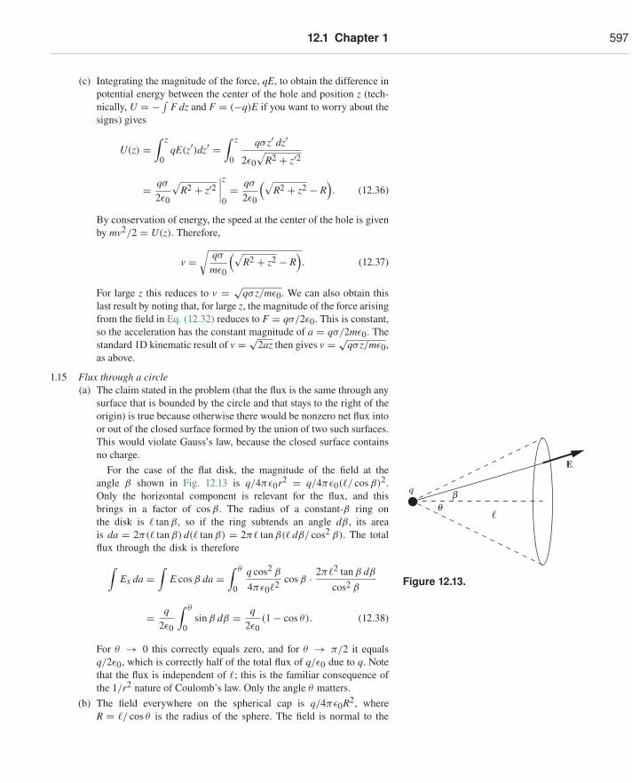
12.1 Chapter 1 597
(c) Integrating the magnitude of the force, qE, to obtain the difference inpotential energy between the center of the hole and position z (tech-nically, U = − ∫
F dz and F = (−q)E if you want to worry about thesigns) gives
U(z) =∫ z
0qE(z′)dz′ =
∫ z
0
qσ z′ dz′
2ε0√
R2 + z′2
= qσ
2ε0
√R2 + z′2
∣∣∣∣z0= qσ
2ε0
(√R2 + z2 − R
). (12.36)
By conservation of energy, the speed at the center of the hole is givenby mv2/2 = U(z). Therefore,
v =√
qσ
mε0
(√R2 + z2 − R
). (12.37)
For large z this reduces to v = √qσ z/mε0. We can also obtain this
last result by noting that, for large z, the magnitude of the force arisingfrom the field in Eq. (12.32) reduces to F = qσ/2ε0. This is constant,so the acceleration has the constant magnitude of a = qσ/2mε0. Thestandard 1D kinematic result of v = √
2az then gives v = √qσ z/mε0,
as above.
1.15 Flux through a circle(a) The claim stated in the problem (that the flux is the same through any
surface that is bounded by the circle and that stays to the right of theorigin) is true because otherwise there would be nonzero net flux intoor out of the closed surface formed by the union of two such surfaces.
bq
q
E
Figure 12.13.
This would violate Gauss’s law, because the closed surface containsno charge.
For the case of the flat disk, the magnitude of the field at theangle β shown in Fig. 12.13 is q/4πε0r2 = q/4πε0(�/ cos β)2.Only the horizontal component is relevant for the flux, and thisbrings in a factor of cos β. The radius of a constant-β ring onthe disk is � tan β, so if the ring subtends an angle dβ, its areais da = 2π(� tan β) d(� tan β) = 2π� tan β(� dβ/ cos2 β). The totalflux through the disk is therefore∫
Ex da =∫
E cos β da =∫ θ
0
q cos2 β
4πε0�2 cos β · 2π�2 tan β dβ
cos2 β
= q2ε0
∫ θ
0sin β dβ = q
2ε0(1 − cos θ). (12.38)
For θ → 0 this correctly equals zero, and for θ → π/2 it equalsq/2ε0, which is correctly half of the total flux of q/ε0 due to q. Notethat the flux is independent of �; this is the familiar consequence ofthe 1/r2 nature of Coulomb’s law. Only the angle θ matters.
(b) The field everywhere on the spherical cap is q/4πε0R2, whereR = �/ cos θ is the radius of the sphere. The field is normal to the
598 Solutions to the problems
sphere, so we don’t have to worry about taking a component. Theradius of a constant-β ring on the cap is R sin β, so the area of thering is 2π(R sin β)(R dβ). The total flux through the spherical cap istherefore∫
E da =∫ θ
0
q4πε0R2 · 2πR2 sin β dβ
= q2ε0
∫ θ
0sin β dβ = q
2ε0(1 − cos θ), (12.39)
in agreement with the result in part (a). The same limiting cases workout, and we can now also consider the θ → π limit (without thesurface crossing the charge, as would happen with the flat disk). Inthis case we have a very small circle on the left side of the origin. Oursphere is nearly a complete sphere, except for a small hole where thecircle is. Equation (12.39) gives a flux of q/ε0 for θ → π , which iscorrectly the total flux due to the charge q.
1.16 Gauss’s law and two point charges(a) The field at position x on the x axis is (dropping terms of order x2)
Ex(x) = q4πε0(� + x)2 − q
4πε0(� − x)2
≈ q4πε0�2
(1
1 + 2x/�− 1
1 − 2x/�
)
≈ q4πε0�2
((1 − 2x/�) − (1 + 2x/�)
)
= − qxπε0�3 . (12.40)
To find the field at position y on the y axis, we must take the verticalcomponent of the fields from the two charges, which brings in a factorof y/
√�2 + y2. The field is therefore (dropping terms of order y2)
Ey(y) = 2 · q4πε0(�2 + y2)
· y√�2 + y2
≈ qy2πε0�3 . (12.41)
The y axis can be chosen to be any axis perpendicular to the line ofthe charges, so this result holds for any point on the perpendicular-bisector plane of the charges.
(b) Although we found the field components in part (a) only for points onthe x axis or on the perpendicular-bisector plane, the results are actu-ally valid for all points in space near the origin. That is, Ex(x, y) ≈−qx/πε0�3, independent of y. And Ey(x, y) ≈ qy/2πε0�3, indepen-dent of x. You can check these facts by writing out the exact expres-sions for the fields. For example, in Eq. (12.41) the � values for thetwo charges become �± x, and this doesn’t change the result, to lead-ing order. Alternatively, note that, due to symmetry, Ex(x, y) is an
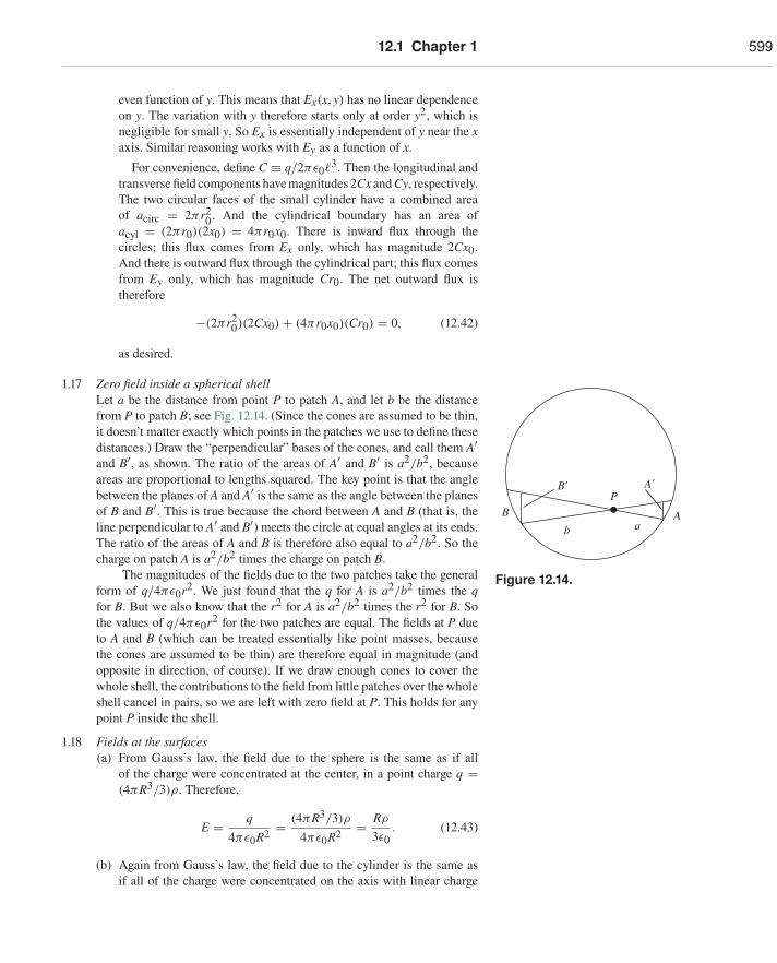
12.1 Chapter 1 599
even function of y. This means that Ex(x, y) has no linear dependenceon y. The variation with y therefore starts only at order y2, which isnegligible for small y. So Ex is essentially independent of y near the xaxis. Similar reasoning works with Ey as a function of x.
For convenience, define C ≡ q/2πε0�3. Then the longitudinal andtransverse field components have magnitudes 2Cx and Cy, respectively.The two circular faces of the small cylinder have a combined areaof acirc = 2πr2
0. And the cylindrical boundary has an area ofacyl = (2πr0)(2x0) = 4πr0x0. There is inward flux through thecircles; this flux comes from Ex only, which has magnitude 2Cx0.And there is outward flux through the cylindrical part; this flux comesfrom Ey only, which has magnitude Cr0. The net outward flux istherefore
−(2πr20)(2Cx0) + (4πr0x0)(Cr0) = 0, (12.42)
as desired.
B�
B
b aA
A�P
Figure 12.14.
1.17 Zero field inside a spherical shellLet a be the distance from point P to patch A, and let b be the distancefrom P to patch B; see Fig. 12.14. (Since the cones are assumed to be thin,it doesn’t matter exactly which points in the patches we use to define thesedistances.) Draw the “perpendicular” bases of the cones, and call them A′and B′, as shown. The ratio of the areas of A′ and B′ is a2/b2, becauseareas are proportional to lengths squared. The key point is that the anglebetween the planes of A and A′ is the same as the angle between the planesof B and B′. This is true because the chord between A and B (that is, theline perpendicular to A′ and B′) meets the circle at equal angles at its ends.The ratio of the areas of A and B is therefore also equal to a2/b2. So thecharge on patch A is a2/b2 times the charge on patch B.
The magnitudes of the fields due to the two patches take the generalform of q/4πε0r2. We just found that the q for A is a2/b2 times the qfor B. But we also know that the r2 for A is a2/b2 times the r2 for B. Sothe values of q/4πε0r2 for the two patches are equal. The fields at P dueto A and B (which can be treated essentially like point masses, becausethe cones are assumed to be thin) are therefore equal in magnitude (andopposite in direction, of course). If we draw enough cones to cover thewhole shell, the contributions to the field from little patches over the wholeshell cancel in pairs, so we are left with zero field at P. This holds for anypoint P inside the shell.
1.18 Fields at the surfaces(a) From Gauss’s law, the field due to the sphere is the same as if all
of the charge were concentrated at the center, in a point charge q =(4πR3/3)ρ. Therefore,
E = q4πε0R2 = (4πR3/3)ρ
4πε0R2 = Rρ
3ε0. (12.43)
(b) Again from Gauss’s law, the field due to the cylinder is the same asif all of the charge were concentrated on the axis with linear charge
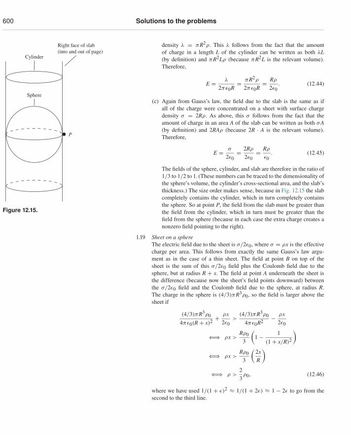
600 Solutions to the problems
density λ = πR2ρ. This λ follows from the fact that the amountof charge in a length L of the cylinder can be written as both λL(by definition) and πR2Lρ (because πR2L is the relevant volume).Therefore,
E = λ
2πε0R= πR2ρ
2πε0R= Rρ
2ε0. (12.44)
(c) Again from Gauss’s law, the field due to the slab is the same as ifall of the charge were concentrated on a sheet with surface chargedensity σ = 2Rρ. As above, this σ follows from the fact that theamount of charge in an area A of the slab can be written as both σA
Right face of slab (into and out of page)
P
Sphere
Cylinder
Figure 12.15.
(by definition) and 2RAρ (because 2R · A is the relevant volume).Therefore,
E = σ
2ε0= 2Rρ
2ε0= Rρ
ε0. (12.45)
The fields of the sphere, cylinder, and slab are therefore in the ratio of1/3 to 1/2 to 1. (These numbers can be traced to the dimensionality ofthe sphere’s volume, the cylinder’s cross-sectional area, and the slab’sthickness.) The size order makes sense, because in Fig. 12.15 the slabcompletely contains the cylinder, which in turn completely containsthe sphere. So at point P, the field from the slab must be greater thanthe field from the cylinder, which in turn must be greater than thefield from the sphere (because in each case the extra charge creates anonzero field pointing to the right).
1.19 Sheet on a sphereThe electric field due to the sheet is σ/2ε0, where σ = ρx is the effectivecharge per area. This follows from exactly the same Gauss’s law argu-ment as in the case of a thin sheet. The field at point B on top of thesheet is the sum of this σ/2ε0 field plus the Coulomb field due to thesphere, but at radius R + x. The field at point A underneath the sheet isthe difference (because now the sheet’s field points downward) betweenthe σ/2ε0 field and the Coulomb field due to the sphere, at radius R.The charge in the sphere is (4/3)πR3ρ0, so the field is larger above thesheet if
(4/3)πR3ρ04πε0(R + x)2 + ρx
2ε0>
(4/3)πR3ρ04πε0R2 − ρx
2ε0
⇐⇒ ρx >Rρ0
3
(1 − 1
(1 + x/R)2
)
⇐⇒ ρx >Rρ0
3
(2xR
)
⇐⇒ ρ >23ρ0, (12.46)
where we have used 1/(1 + ε)2 ≈ 1/(1 + 2ε) ≈ 1 − 2ε to go from thesecond to the third line.
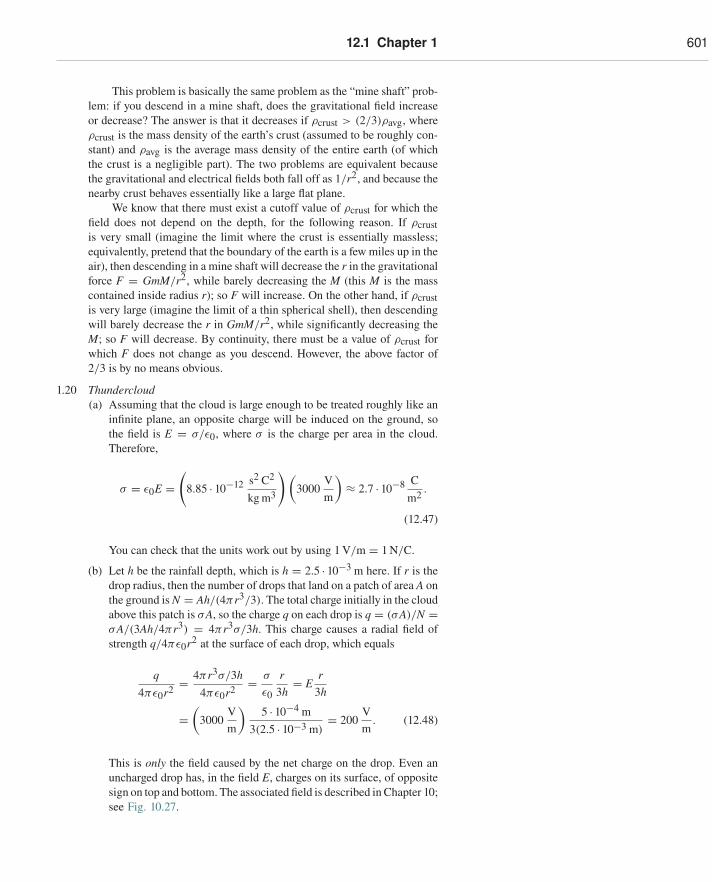
12.1 Chapter 1 601
This problem is basically the same problem as the “mine shaft” prob-lem: if you descend in a mine shaft, does the gravitational field increaseor decrease? The answer is that it decreases if ρcrust > (2/3)ρavg, whereρcrust is the mass density of the earth’s crust (assumed to be roughly con-stant) and ρavg is the average mass density of the entire earth (of whichthe crust is a negligible part). The two problems are equivalent becausethe gravitational and electrical fields both fall off as 1/r2, and because thenearby crust behaves essentially like a large flat plane.
We know that there must exist a cutoff value of ρcrust for which thefield does not depend on the depth, for the following reason. If ρcrustis very small (imagine the limit where the crust is essentially massless;equivalently, pretend that the boundary of the earth is a few miles up in theair), then descending in a mine shaft will decrease the r in the gravitationalforce F = GmM/r2, while barely decreasing the M (this M is the masscontained inside radius r); so F will increase. On the other hand, if ρcrustis very large (imagine the limit of a thin spherical shell), then descendingwill barely decrease the r in GmM/r2, while significantly decreasing theM; so F will decrease. By continuity, there must be a value of ρcrust forwhich F does not change as you descend. However, the above factor of2/3 is by no means obvious.
1.20 Thundercloud(a) Assuming that the cloud is large enough to be treated roughly like an
infinite plane, an opposite charge will be induced on the ground, sothe field is E = σ/ε0, where σ is the charge per area in the cloud.Therefore,
σ = ε0E =(
8.85 · 10−12 s2 C2
kg m3
)(3000
Vm
)≈ 2.7 · 10−8 C
m2 .
(12.47)
You can check that the units work out by using 1 V/m = 1 N/C.
(b) Let h be the rainfall depth, which is h = 2.5 · 10−3 m here. If r is thedrop radius, then the number of drops that land on a patch of area A onthe ground is N = Ah/(4πr3/3). The total charge initially in the cloudabove this patch is σA, so the charge q on each drop is q = (σA)/N =σA/(3Ah/4πr3) = 4πr3σ/3h. This charge causes a radial field ofstrength q/4πε0r2 at the surface of each drop, which equals
q4πε0r2 = 4πr3σ/3h
4πε0r2 = σ
ε0
r3h
= Er
3h
=(
3000Vm
)5 · 10−4 m
3(2.5 · 10−3 m)= 200
Vm
. (12.48)
This is only the field caused by the net charge on the drop. Even anuncharged drop has, in the field E, charges on its surface, of oppositesign on top and bottom. The associated field is described in Chapter 10;see Fig. 10.27.
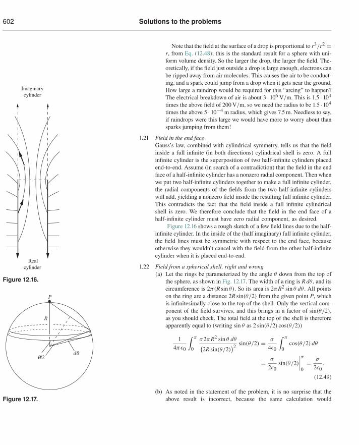
602 Solutions to the problems
Note that the field at the surface of a drop is proportional to r3/r2 =r, from Eq. (12.48); this is the standard result for a sphere with uni-form volume density. So the larger the drop, the larger the field. The-oretically, if the field just outside a drop is large enough, electrons canbe ripped away from air molecules. This causes the air to be conduct-ing, and a spark could jump from a drop when it gets near the ground.How large a raindrop would be required for this “arcing” to happen?The electrical breakdown of air is about 3 · 106 V/m. This is 1.5 · 104
times the above field of 200 V/m, so we need the radius to be 1.5 ·104
Realcylinder
Imaginarycylinder
Figure 12.16.
times the above 5 · 10−4 m radius, which gives 7.5 m. Needless to say,if raindrops were this large we would have more to worry about thansparks jumping from them!
1.21 Field in the end faceGauss’s law, combined with cylindrical symmetry, tells us that the fieldinside a full infinite (in both directions) cylindrical shell is zero. A fullinfinite cylinder is the superposition of two half-infinite cylinders placedend-to-end. Assume (in search of a contradiction) that the field in the endface of a half-infinite cylinder has a nonzero radial component. Then whenwe put two half-infinite cylinders together to make a full infinite cylinder,the radial components of the fields from the two half-infinite cylinderswill add, yielding a nonzero field inside the resulting full infinite cylinder.This contradicts the fact that the field inside a full infinite cylindricalshell is zero. We therefore conclude that the field in the end face of ahalf-infinite cylinder must have zero radial component, as desired.
Figure 12.16 shows a rough sketch of a few field lines due to the half-infinite cylinder. In the inside of the (half imaginary) full infinite cylinder,the field lines must be symmetric with respect to the end face, becauseotherwise they wouldn’t cancel with the field from the other half-infinitecylinder when it is placed end-to-end.
1.22 Field from a spherical shell, right and wrong(a) Let the rings be parameterized by the angle θ down from the top of
the sphere, as shown in Fig. 12.17. The width of a ring is R dθ , and its
q/2dq
R
P
Figure 12.17.
circumference is 2π(R sin θ). So its area is 2πR2 sin θ dθ . All pointson the ring are a distance 2R sin(θ/2) from the given point P, whichis infinitesimally close to the top of the shell. Only the vertical com-ponent of the field survives, and this brings in a factor of sin(θ/2),as you should check. The total field at the top of the shell is thereforeapparently equal to (writing sin θ as 2 sin(θ/2) cos(θ/2))
14πε0
∫ π
0
σ2πR2 sin θ dθ(2R sin(θ/2)
)2 sin(θ/2) = σ
4ε0
∫ π
0cos(θ/2) dθ
= σ
2ε0sin(θ/2)
∣∣∣∣π0= σ
2ε0.
(12.49)
(b) As noted in the statement of the problem, it is no surprise that theabove result is incorrect, because the same calculation would
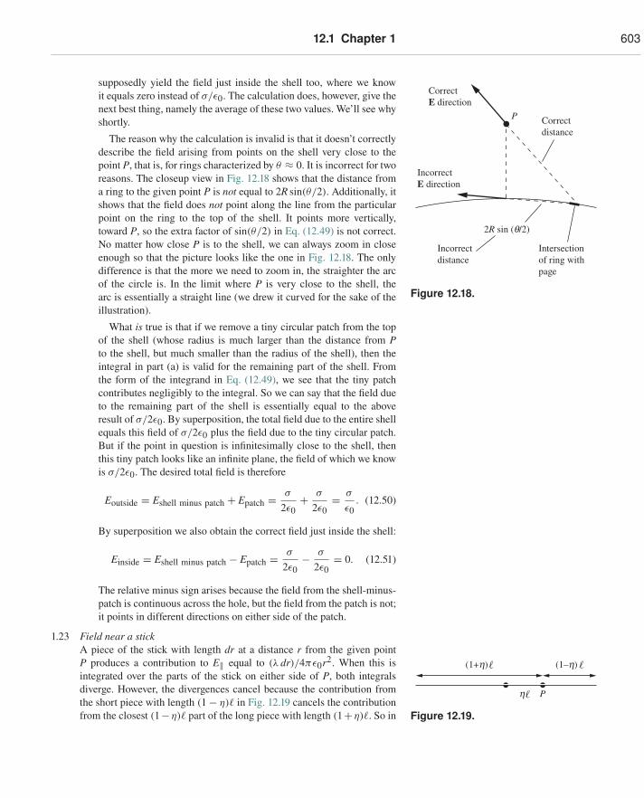
12.1 Chapter 1 603
supposedly yield the field just inside the shell too, where we knowit equals zero instead of σ/ε0. The calculation does, however, give thenext best thing, namely the average of these two values. We’ll see whyshortly.
The reason why the calculation is invalid is that it doesn’t correctlydescribe the field arising from points on the shell very close to thepoint P, that is, for rings characterized by θ ≈ 0. It is incorrect for tworeasons. The closeup view in Fig. 12.18 shows that the distance froma ring to the given point P is not equal to 2R sin(θ/2). Additionally, itshows that the field does not point along the line from the particular
2R sin (q/2)
P
Intersectionof ring withpage
CorrectE direction
IncorrectE direction
Correct distance
Incorrect distance
Figure 12.18.
point on the ring to the top of the shell. It points more vertically,toward P, so the extra factor of sin(θ/2) in Eq. (12.49) is not correct.No matter how close P is to the shell, we can always zoom in closeenough so that the picture looks like the one in Fig. 12.18. The onlydifference is that the more we need to zoom in, the straighter the arcof the circle is. In the limit where P is very close to the shell, thearc is essentially a straight line (we drew it curved for the sake of theillustration).
What is true is that if we remove a tiny circular patch from the topof the shell (whose radius is much larger than the distance from Pto the shell, but much smaller than the radius of the shell), then theintegral in part (a) is valid for the remaining part of the shell. Fromthe form of the integrand in Eq. (12.49), we see that the tiny patchcontributes negligibly to the integral. So we can say that the field dueto the remaining part of the shell is essentially equal to the aboveresult of σ/2ε0. By superposition, the total field due to the entire shellequals this field of σ/2ε0 plus the field due to the tiny circular patch.But if the point in question is infinitesimally close to the shell, thenthis tiny patch looks like an infinite plane, the field of which we knowis σ/2ε0. The desired total field is therefore
Eoutside = Eshell minus patch + Epatch = σ
2ε0+ σ
2ε0= σ
ε0. (12.50)
By superposition we also obtain the correct field just inside the shell:
Einside = Eshell minus patch − Epatch = σ
2ε0− σ
2ε0= 0. (12.51)
The relative minus sign arises because the field from the shell-minus-patch is continuous across the hole, but the field from the patch is not;it points in different directions on either side of the patch.
1.23 Field near a stickA piece of the stick with length dr at a distance r from the given pointP produces a contribution to E‖ equal to (λ dr)/4πε0r2. When this is
Ph
(1+h) (1–h)
Figure 12.19.
integrated over the parts of the stick on either side of P, both integralsdiverge. However, the divergences cancel because the contribution fromthe short piece with length (1 − η)� in Fig. 12.19 cancels the contributionfrom the closest (1−η)� part of the long piece with length (1+η)�. So in
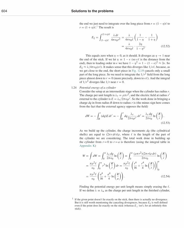
604 Solutions to the problems
the end we just need to integrate over the long piece from r = (1 − η)� tor = (1 + η)�.1 The result is
E‖ =∫ (1+η)�
(1−η)�
λ dr4πε0r2 = λ
4πε0�
(1
1 − η− 1
1 + η
)
= λ
4πε0�· 2η
1 − η2 . (12.52)
This equals zero when η = 0, as it should. It diverges as η → 1 nearthe end of the stick. If we let η ≡ 1 − ε (so ε� is the distance from theend), then to leading order in ε we have 1 − η2 = 1 − (1 − ε)2 ≈ 2ε. SoE‖ ≈ λ/4πε0(ε�). It makes sense that this diverges like 1/ε�, because, aswe get close to the end, the short piece in Fig. 12.19 cancels only a smallpart of the long piece. So we need to integrate the 1/r2 field from the longpiece almost down to r = 0 (more precisely, down to ε�). And the integralof 1/r2 diverges like 1/r near r = 0.
1.24 Potential energy of a cylinderConsider the setup at an intermediate stage when the cylinder has radius r.The charge per unit length is λr = ρπr2, and the electric field at radius r′external to the cylinder is E = λr/2πε0r′. So the work done in bringing acharge dq in from radius R down to radius r is (the minus sign here comesfrom the fact that the external agency opposes the field)
dW = −∫ r
R(dq)E dr′ = −
∫ r
Rdq
λr
2πε0r′ dr′ = λr dq2πε0
ln(
Rr
).
(12.53)
As we build up the cylinder, the charge increments dq (the cylindricalshells) are equal to (2πr dr)�ρ, where � is the length of the part ofthe cylinder we are considering. The total work done in building upthe cylinder from r= 0 to r= a is therefore (using the integral table inAppendix K)
W =∫
dW =∫ a
0
λr dq2πε0
ln(
Rr
)=
∫ a
0
(ρπr2)(2πr�ρ dr)2πε0
ln(
Rr
)
= πρ2�
ε0
∫ a
0r3 ln
(Rr
)dr = πρ2�
ε0
(r4
16+ r4
4ln
(Rr
))∣∣∣∣∣a
0
= πρ2�
ε0
(a4
16+ a4
4ln
(Ra
)). (12.54)
Finding the potential energy per unit length means simply erasing the �.If we define λ ≡ λa as the charge per unit length in the finished cylinder,
1 If the given point doesn’t lie exactly on the stick, then there is actually no divergence.But it is still worth mentioning the canceling divergences, because E‖ is well definedeven if the point does lie exactly on the stick (whereas E⊥ isn’t, for an infinitely thinstick).
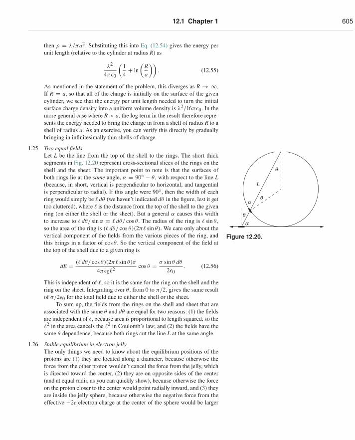
12.1 Chapter 1 605
then ρ = λ/πa2. Substituting this into Eq. (12.54) gives the energy perunit length (relative to the cylinder at radius R) as
λ2
4πε0
(14+ ln
(Ra
)). (12.55)
As mentioned in the statement of the problem, this diverges as R → ∞.If R = a, so that all of the charge is initially on the surface of the givencylinder, we see that the energy per unit length needed to turn the initialsurface charge density into a uniform volume density is λ2/16πε0. In themore general case where R > a, the log term in the result therefore repre-sents the energy needed to bring the charge in from a shell of radius R to ashell of radius a. As an exercise, you can verify this directly by graduallybringing in infinitesimally thin shells of charge.
1.25 Two equal fieldsLet L be the line from the top of the shell to the rings. The short thicksegments in Fig. 12.20 represent cross-sectional slices of the rings on the
q
q
qa
a
L
Figure 12.20.
shell and the sheet. The important point to note is that the surfaces ofboth rings lie at the same angle, α = 90◦ − θ , with respect to the line L(because, in short, vertical is perpendicular to horizontal, and tangentialis perpendicular to radial). If this angle were 90◦, then the width of eachring would simply be � dθ (we haven’t indicated dθ in the figure, lest it gettoo cluttered), where � is the distance from the top of the shell to the givenring (on either the shell or the sheet). But a general α causes this widthto increase to � dθ/ sin α = � dθ/ cos θ . The radius of the ring is � sin θ ,so the area of the ring is (� dθ/ cos θ)(2π� sin θ). We care only about thevertical component of the fields from the various pieces of the ring, andthis brings in a factor of cos θ . So the vertical component of the field atthe top of the shell due to a given ring is
dE = (� dθ/ cos θ)(2π� sin θ)σ
4πε0�2 cos θ = σ sin θ dθ
2ε0. (12.56)
This is independent of �, so it is the same for the ring on the shell and thering on the sheet. Integrating over θ , from 0 to π/2, gives the same resultof σ/2ε0 for the total field due to either the shell or the sheet.
To sum up, the fields from the rings on the shell and sheet that areassociated with the same θ and dθ are equal for two reasons: (1) the fieldsare independent of �, because area is proportional to length squared, so the�2 in the area cancels the �2 in Coulomb’s law; and (2) the fields have thesame θ dependence, because both rings cut the line L at the same angle.
1.26 Stable equilibrium in electron jellyThe only things we need to know about the equilibrium positions of theprotons are (1) they are located along a diameter, because otherwise theforce from the other proton wouldn’t cancel the force from the jelly, whichis directed toward the center, (2) they are on opposite sides of the center(and at equal radii, as you can quickly show), because otherwise the forceon the proton closer to the center would point radially inward, and (3) theyare inside the jelly sphere, because otherwise the negative force from theeffective −2e electron charge at the center of the sphere would be larger
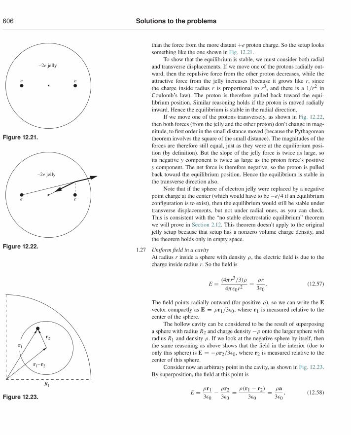
606 Solutions to the problems
than the force from the more distant +e proton charge. So the setup lookssomething like the one shown in Fig. 12.21.
–2e jelly
ee
Figure 12.21.
To show that the equilibrium is stable, we must consider both radialand transverse displacements. If we move one of the protons radially out-ward, then the repulsive force from the other proton decreases, while theattractive force from the jelly increases (because it grows like r, sincethe charge inside radius r is proportional to r3, and there is a 1/r2 inCoulomb’s law). The proton is therefore pulled back toward the equi-librium position. Similar reasoning holds if the proton is moved radiallyinward. Hence the equilibrium is stable in the radial direction.
If we move one of the protons transversely, as shown in Fig. 12.22,then both forces (from the jelly and the other proton) don’t change in mag-nitude, to first order in the small distance moved (because the Pythagoreantheorem involves the square of the small distance). The magnitudes of theforces are therefore still equal, just as they were at the equilibrium posi-
ee
–2e jelly
Figure 12.22.
tion (by definition). But the slope of the jelly force is twice as large, soits negative y component is twice as large as the proton force’s positivey component. The net force is therefore negative, so the proton is pulledback toward the equilibrium position. Hence the equilibrium is stable inthe transverse direction also.
Note that if the sphere of electron jelly were replaced by a negativepoint charge at the center (which would have to be −e/4 if an equilibriumconfiguration is to exist), then the equilibrium would still be stable undertransverse displacements, but not under radial ones, as you can check.This is consistent with the “no stable electrostatic equilibrium” theoremwe will prove in Section 2.12. This theorem doesn’t apply to the originaljelly setup because that setup has a nonzero volume charge density, andthe theorem holds only in empty space.
1.27 Uniform field in a cavityAt radius r inside a sphere with density ρ, the electric field is due to thecharge inside radius r. So the field is
E = (4πr3/3)ρ
4πε0r2 = ρr3ε0
. (12.57)
The field points radially outward (for positive ρ), so we can write the E
R1
r1– r2
r2
r1
Figure 12.23.
vector compactly as E = ρr1/3ε0, where r1 is measured relative to thecenter of the sphere.
The hollow cavity can be considered to be the result of superposinga sphere with radius R2 and charge density −ρ onto the larger sphere withradius R1 and density ρ. If we look at the negative sphere by itself, thenthe same reasoning as above shows that the field in the interior (due toonly this sphere) is E = −ρr2/3ε0, where r2 is measured relative to thecenter of this sphere.
Consider now an arbitrary point in the cavity, as shown in Fig. 12.23.By superposition, the field at this point is
E = ρr13ε0
− ρr23ε0
= ρ(r1 − r2)
3ε0= ρa
3ε0, (12.58)
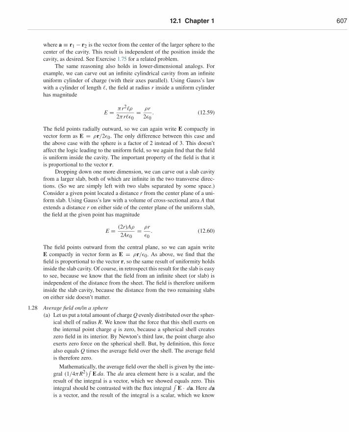
12.1 Chapter 1 607
where a ≡ r1 − r2 is the vector from the center of the larger sphere to thecenter of the cavity. This result is independent of the position inside thecavity, as desired. See Exercise 1.75 for a related problem.
The same reasoning also holds in lower-dimensional analogs. Forexample, we can carve out an infinite cylindrical cavity from an infiniteuniform cylinder of charge (with their axes parallel). Using Gauss’s lawwith a cylinder of length �, the field at radius r inside a uniform cylinderhas magnitude
E = πr2�ρ
2πr�ε0= ρr
2ε0. (12.59)
The field points radially outward, so we can again write E compactly invector form as E = ρr/2ε0. The only difference between this case andthe above case with the sphere is a factor of 2 instead of 3. This doesn’taffect the logic leading to the uniform field, so we again find that the fieldis uniform inside the cavity. The important property of the field is that itis proportional to the vector r.
Dropping down one more dimension, we can carve out a slab cavityfrom a larger slab, both of which are infinite in the two transverse direc-tions. (So we are simply left with two slabs separated by some space.)Consider a given point located a distance r from the center plane of a uni-form slab. Using Gauss’s law with a volume of cross-sectional area A thatextends a distance r on either side of the center plane of the uniform slab,the field at the given point has magnitude
E = (2r)Aρ
2Aε0= ρr
ε0. (12.60)
The field points outward from the central plane, so we can again writeE compactly in vector form as E = ρr/ε0. As above, we find that thefield is proportional to the vector r, so the same result of uniformity holdsinside the slab cavity. Of course, in retrospect this result for the slab is easyto see, because we know that the field from an infinite sheet (or slab) isindependent of the distance from the sheet. The field is therefore uniforminside the slab cavity, because the distance from the two remaining slabson either side doesn’t matter.
1.28 Average field on/in a sphere(a) Let us put a total amount of charge Q evenly distributed over the spher-
ical shell of radius R. We know that the force that this shell exerts onthe internal point charge q is zero, because a spherical shell createszero field in its interior. By Newton’s third law, the point charge alsoexerts zero force on the spherical shell. But, by definition, this forcealso equals Q times the average field over the shell. The average fieldis therefore zero.
Mathematically, the average field over the shell is given by the inte-gral (1/4πR2)
∫E da. The da area element here is a scalar, and the
result of the integral is a vector, which we showed equals zero. Thisintegral should be contrasted with the flux integral
∫E · da. Here da
is a vector, and the result of the integral is a scalar, which we know
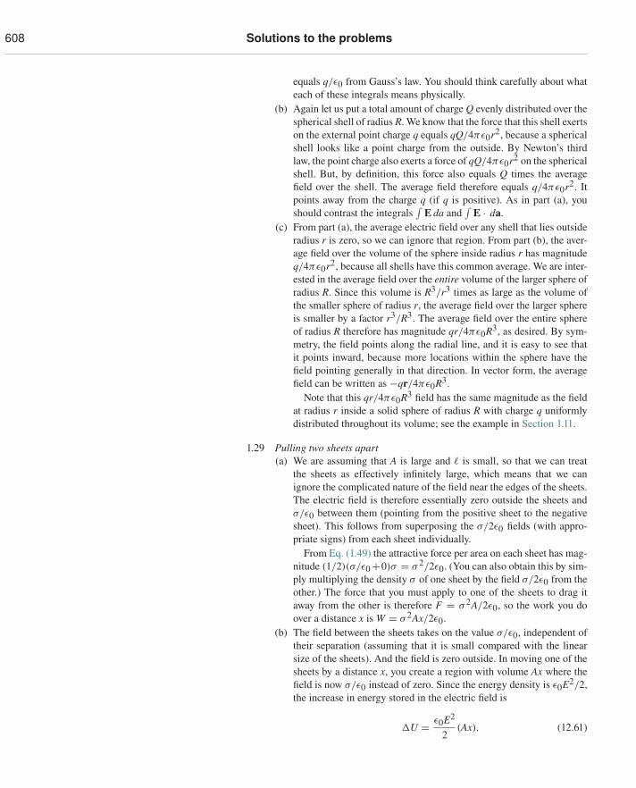
608 Solutions to the problems
equals q/ε0 from Gauss’s law. You should think carefully about whateach of these integrals means physically.
(b) Again let us put a total amount of charge Q evenly distributed over thespherical shell of radius R. We know that the force that this shell exertson the external point charge q equals qQ/4πε0r2, because a sphericalshell looks like a point charge from the outside. By Newton’s thirdlaw, the point charge also exerts a force of qQ/4πε0r2 on the sphericalshell. But, by definition, this force also equals Q times the averagefield over the shell. The average field therefore equals q/4πε0r2. Itpoints away from the charge q (if q is positive). As in part (a), youshould contrast the integrals
∫E da and
∫E · da.
(c) From part (a), the average electric field over any shell that lies outsideradius r is zero, so we can ignore that region. From part (b), the aver-age field over the volume of the sphere inside radius r has magnitudeq/4πε0r2, because all shells have this common average. We are inter-ested in the average field over the entire volume of the larger sphere ofradius R. Since this volume is R3/r3 times as large as the volume ofthe smaller sphere of radius r, the average field over the larger sphereis smaller by a factor r3/R3. The average field over the entire sphereof radius R therefore has magnitude qr/4πε0R3, as desired. By sym-metry, the field points along the radial line, and it is easy to see thatit points inward, because more locations within the sphere have thefield pointing generally in that direction. In vector form, the averagefield can be written as −qr/4πε0R3.
Note that this qr/4πε0R3 field has the same magnitude as the fieldat radius r inside a solid sphere of radius R with charge q uniformlydistributed throughout its volume; see the example in Section 1.11.
1.29 Pulling two sheets apart(a) We are assuming that A is large and � is small, so that we can treat
the sheets as effectively infinitely large, which means that we canignore the complicated nature of the field near the edges of the sheets.The electric field is therefore essentially zero outside the sheets andσ/ε0 between them (pointing from the positive sheet to the negativesheet). This follows from superposing the σ/2ε0 fields (with appro-priate signs) from each sheet individually.
From Eq. (1.49) the attractive force per area on each sheet has mag-nitude (1/2)(σ/ε0+0)σ = σ 2/2ε0. (You can also obtain this by sim-ply multiplying the density σ of one sheet by the field σ/2ε0 from theother.) The force that you must apply to one of the sheets to drag itaway from the other is therefore F = σ 2A/2ε0, so the work you doover a distance x is W = σ 2Ax/2ε0.
(b) The field between the sheets takes on the value σ/ε0, independent oftheir separation (assuming that it is small compared with the linearsize of the sheets). And the field is zero outside. In moving one of thesheets by a distance x, you create a region with volume Ax where thefield is now σ/ε0 instead of zero. Since the energy density is ε0E2/2,the increase in energy stored in the electric field is
�U = ε0E2
2(Ax). (12.61)
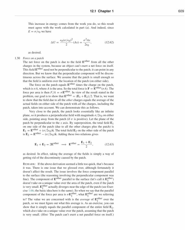
12.1 Chapter 1 609
This increase in energy comes from the work you do, so this resultmust agree with the work calculated in part (a). And indeed, sinceE = σ/ε0 we have
�U = ε0(σ/ε0)2
2(Ax) = σ 2Ax
2ε0, (12.62)
as desired.
1.30 Force on a patchThe net force on the patch is due to the field Eother from all the othercharges in the system, because an object can’t exert a net force on itself.This field Eother need not be perpendicular to the patch; it can point in anydirection. But we know that the perpendicular component will be discon-tinuous across the surface. We assume that the patch is small enough sothat the field is uniform over the location of the patch (on either side).
The force on the patch equals Eother times the charge on the patch,which is σA, where A is the area. So the total force is F = Eother(σA). Theforce per area is then F/A = σEother. In view of the result stated in theproblem, our goal is to show that Eother = (E1 + E2)/2. That is, we wantto show that the field due to all the other charges equals the average of theactual fields on either side of the patch with all the charges, including thepatch, taken into account. We can demonstrate this as follows.
Very close to the patch, the patch looks essentially like an infiniteplane, so it produces a perpendicular field with magnitude σ/2ε0 on eitherside, pointing away from the patch (if σ is positive). Let the plane of thepatch be perpendicular to the x axis. By superposition, the total field E1on one side of the patch (due to all the other charges plus the patch) isE1 = Eother + (σ/2ε0)x. The total field E2 on the other side of the patchis E2 = Eother − (σ/2ε0)x. Adding these two relations gives
E1 + E2 = 2Eother �⇒ Eother = E1 + E22
, (12.63)
as desired. In effect, taking the average of the fields is simply a way ofgetting rid of the discontinuity caused by the patch.
REMARK: If the above derivation seemed a little too quick, that’s becauseit was. There is one issue that we glossed over, although fortunately itdoesn’t affect the result. The issue involves the force component parallelto the surface (the reasoning involving the perpendicular component wasfine). The component of Eother parallel to the surface (let’s call it Eother‖ )doesn’t take on a unique value over the area of the patch, even if the patchis very small. Eother‖ actually diverges near the edge of the patch (see Exer-cise 1.66; the basic idea here is the same). So when we say that the parallelcomponent of the force per area is σEother‖ , what Eother‖ are we referring
to? The value we are concerned with is the average of Eother‖ over thepatch, so we must figure out what this average is. As an exercise, you canshow that it simply equals the parallel component of the entire field E‖,which does take on a unique value over the patch, assuming that the patchis very small. (Hint: The patch can’t exert a net parallel force on itself.)
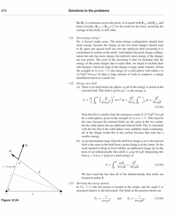
610 Solutions to the problems
But E‖ is continuous across the patch, so it equals both E1,‖ and E2,‖, andhence trivially (E1,‖ + E2,‖)/2. So the result for the force, involving theaverage of the fields, is still valid.
1.31 Decreasing energy?No, it doesn’t make sense. The point-charge configuration should havemore energy, because the charge on the two point charges should wantto fly apart and spread itself out over the spherical shell (assuming it isconstrained to remain on the shell). And indeed, the point-charge configu-ration not only has more energy, but infinitely more energy, if the chargesare true points. The error in the reasoning is that we included only theenergy of the point charges due to each other; we forgot to include theirself-energies, which are large if the charges occupy small volumes. (Fromthe example in Section 1.15, the energy of a solid sphere with radius a is(3/5)Q2/4πε0a.) It takes a large amount of work to compress a chargedistribution down to a small size.
1.32 Energy of a shell(a) There is no field inside the sphere, so all of the energy is stored in the
external field. This field is Q/4πε0r2, so the energy is
U = ε02
∫ ∞R
(Q
4πε0r2
)24πr2 dr = Q2
8πε0
∫ ∞R
1r2 dr = Q2
8πε0R.
(12.64)
Note that this is smaller than the analogous result of (3/5)Q2/4πε0Rfor a solid sphere, given in the example in Section 1.15. This must bethe case, because the external fields are the same in the two setups,but the solid sphere has an additional internal field. This is consistentwith the fact that if the solid sphere were suddenly made conducting,all of the charge would flee to the surface because that state has asmaller energy.
(b) At an intermediate stage when the shell has charge q on it, the externalfield is the same as the field from a point charge q at the center. So thework needed to bring in from infinity an additional charge dq (in theform of an infinitesimally thin shell) is q dq/4πε0R. Integrating thisfrom q = 0 to q = Q gives a total energy of
U =∫ Q
0
q dq4πε0R
= Q2
8πε0R. (12.65)
q
y
R
E1
E2
r
r – b cos q
be e
Figure 12.24.
We have used the fact that all of the infinitesimally thin shells arelocated at radius R.
1.33 Deriving the energy densityIn Fig. 12.24 the left proton is located at the origin, and the angle θ ismeasured relative to the horizontal. The fields at the position shown are
E1 = e4πε0r2 and E2 = e
4πε0R2 , (12.66)
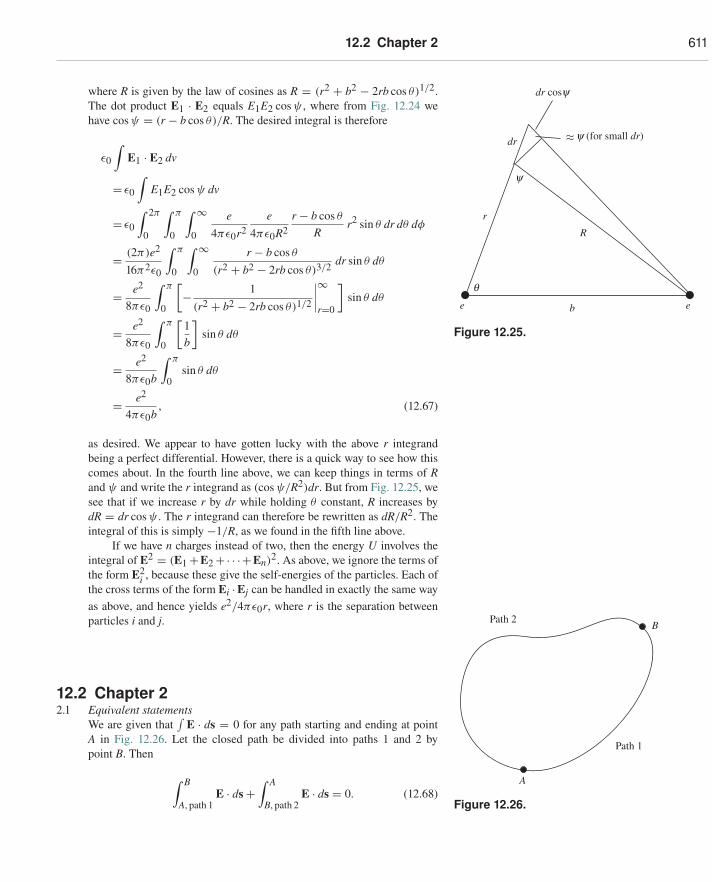
12.2 Chapter 2 611
where R is given by the law of cosines as R = (r2 + b2 − 2rb cos θ)1/2.The dot product E1 · E2 equals E1E2 cos ψ , where from Fig. 12.24 wehave cos ψ = (r − b cos θ)/R. The desired integral is therefore
ε0
∫E1 · E2 dv
= ε0
∫E1E2 cos ψ dv
= ε0
∫ 2π
0
∫ π
0
∫ ∞0
e4πε0r2
e4πε0R2
r − b cos θ
Rr2 sin θ dr dθ dφ
= (2π)e2
16π2ε0
∫ π
0
∫ ∞0
r − b cos θ
(r2 + b2 − 2rb cos θ)3/2 dr sin θ dθ
= e2
8πε0
∫ π
0
[− 1
(r2 + b2 − 2rb cos θ)1/2
∣∣∣∣∞r=0
]sin θ dθ
= e2
8πε0
∫ π
0
[1b
]sin θ dθ
= e2
8πε0b
∫ π
0sin θ dθ
= e2
4πε0b, (12.67)
q
y
R
r
dr
dr cosy
be e
y (for small dr)
Figure 12.25.
as desired. We appear to have gotten lucky with the above r integrandbeing a perfect differential. However, there is a quick way to see how thiscomes about. In the fourth line above, we can keep things in terms of Rand ψ and write the r integrand as (cos ψ/R2)dr. But from Fig. 12.25, wesee that if we increase r by dr while holding θ constant, R increases bydR = dr cos ψ . The r integrand can therefore be rewritten as dR/R2. Theintegral of this is simply −1/R, as we found in the fifth line above.
If we have n charges instead of two, then the energy U involves theintegral of E2 = (E1 +E2 +· · ·+En)2. As above, we ignore the terms ofthe form E2
i , because these give the self-energies of the particles. Each ofthe cross terms of the form Ei ·Ej can be handled in exactly the same wayas above, and hence yields e2/4πε0r, where r is the separation betweenparticles i and j. B
A
Path 1
Path 2
Figure 12.26.
12.2 Chapter 22.1 Equivalent statements
We are given that∫
E · ds = 0 for any path starting and ending at pointA in Fig. 12.26. Let the closed path be divided into paths 1 and 2 bypoint B. Then
∫ B
A, path 1E · ds +
∫ A
B, path 2E · ds = 0. (12.68)
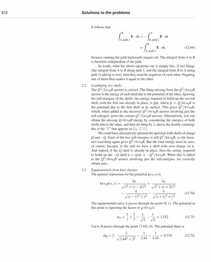
612 Solutions to the problems
It follows that ∫ B
A, path 1E · ds = −
∫ A
B, path 2E · ds
=∫ B
A, path 2E · ds, (12.69)
because running the path backwards negates ds. The integral from A to Bis therefore independent of the path.
In words, what the above equations say is simply this: if two things(the integral from A to B along path 1, and the integral from B to A alongpath 2) add up to zero, then they must be negatives of each other. Negatingone of them then makes it equal to the other.
2.2 Combining two shellsThe Q2/2πε0R answer is correct. The thing missing from the Q2/4πε0Ranswer is the energy of each shell due to the potential of the other. Ignoringthe self-energies of the shells, the energy required to build up the secondshell, with the first one already in place, is Qφ, where φ = Q/4πε0R isthe potential due to the first shell at its surface. This gives Q2/4πε0R,which, when added to the incorrect Q2/4πε0R answer involving just theself-energies, gives the correct Q2/2πε0R answer. Alternatively, you canobtain the missing Q/4πε0R energy by considering the energies of bothshells due to the other, and then dividing by 2, due to the double counting;this is the “2” that appears in Eq. (2.32).
We could have alternatively phrased the question with shells of chargeQ and −Q. Each of the two self-energies is still Q2/8πε0R, so the incor-rect reasoning again gives Q2/4πε0R. But the total energy must be zero,of course, because in the end we have a shell with zero charge on it.And indeed, if the Q shell is already in place, then the energy requiredto build up the −Q shell is (−Q)φ = −Q2/4πε0R. When this is addedto the Q2/4πε0R answer involving just the self-energies, we correctlyobtain zero.
2.3 Equipotentials from four chargesThe general expression for the potential φ(x, y) is
4πε0φ(x, y) = 2q√x2 + (y − 2�)2
+ 2q√x2 + (y + 2�)2
− q√(x − �)2 + y2
− q√(x + �)2 + y2
. (12.70)
The equipotential curve A passes through the point (0, �). The potential atthis point is (ignoring the factor of q/4πε0�)
φA = 21+ 2
3− 1√
2− 1√
2= 1.252. (12.71)
Curve B passes through the point (3.44�, 0). The potential there is
φB = 2 · 2√3.442 + 22
− 12.44
− 14.44
= 0.370. (12.72)
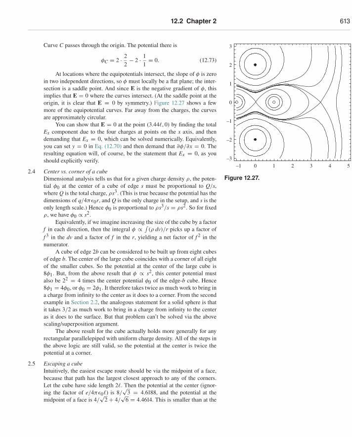
12.2 Chapter 2 613
Curve C passes through the origin. The potential there is
φC = 2 · 22− 2 · 1
1= 0. (12.73)
At locations where the equipotentials intersect, the slope of φ is zeroin two independent directions, so φ must locally be a flat plane; the inter-
–1 0 1 2 3 4 5–3
–2
–1
0
1
2
3
Figure 12.27.
section is a saddle point. And since E is the negative gradient of φ, thisimplies that E = 0 where the curves intersect. (At the saddle point at theorigin, it is clear that E = 0 by symmetry.) Figure 12.27 shows a fewmore of the equipotential curves. Far away from the charges, the curvesare approximately circular.
You can show that E = 0 at the point (3.44�, 0) by finding the totalEx component due to the four charges at points on the x axis, and thendemanding that Ex = 0, which can be solved numerically. Equivalently,you can set y = 0 in Eq. (12.70) and then demand that ∂φ/∂x = 0. Theresulting equation will, of course, be the statement that Ex = 0, as youshould explicitly verify.
2.4 Center vs. corner of a cubeDimensional analysis tells us that for a given charge density ρ, the poten-tial φ0 at the center of a cube of edge s must be proportional to Q/s,where Q is the total charge, ρs3. (This is true because the potential has thedimensions of q/4πε0r, and Q is the only charge in the setup, and s is theonly length scale.) Hence φ0 is proportional to ρs3/s = ρs2. So for fixedρ, we have φ0 ∝ s2.
Equivalently, if we imagine increasing the size of the cube by a factorf in each direction, then the integral φ ∝ ∫
(ρ dv)/r picks up a factor off 3 in the dv and a factor of f in the r, yielding a net factor of f 2 in thenumerator.
A cube of edge 2b can be considered to be built up from eight cubesof edge b. The center of the large cube coincides with a corner of all eightof the smaller cubes. So the potential at the center of the large cube is8φ1. But, from the above result that φ ∝ s2, this center potential mustalso be 22 = 4 times the center potential φ0 of the edge-b cube. Hence8φ1 = 4φ0, or φ0 = 2φ1. It therefore takes twice as much work to bring ina charge from infinity to the center as it does to a corner. From the secondexample in Section 2.2, the analogous statement for a solid sphere is thatit takes 3/2 as much work to bring in a charge from infinity to the centeras it does to the surface. But that problem can’t be solved via the abovescaling/superposition argument.
The above result for the cube actually holds more generally for anyrectangular parallelepiped with uniform charge density. All of the steps inthe above logic are still valid, so the potential at the center is twice thepotential at a corner.
2.5 Escaping a cubeIntuitively, the easiest escape route should be via the midpoint of a face,because that path has the largest closest approach to any of the corners.Let the cube have side length 2�. Then the potential at the center (ignor-ing the factor of e/4πε0�) is 8/
√3 = 4.6188, and the potential at the
midpoint of a face is 4/√
2 + 4/√
6 = 4.4614. This is smaller than at the
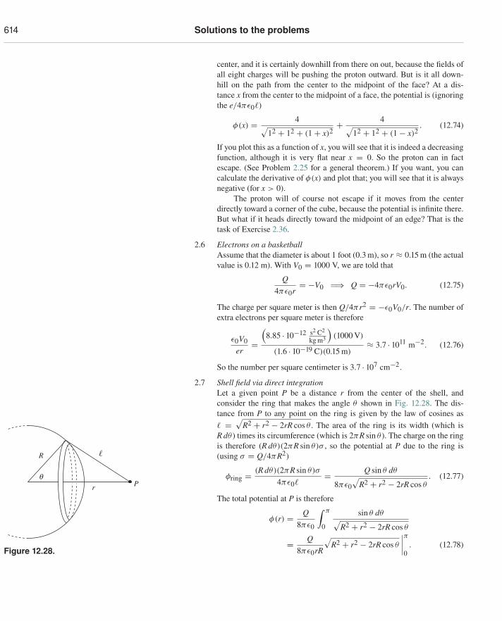
614 Solutions to the problems
center, and it is certainly downhill from there on out, because the fields ofall eight charges will be pushing the proton outward. But is it all down-hill on the path from the center to the midpoint of the face? At a dis-tance x from the center to the midpoint of a face, the potential is (ignoringthe e/4πε0�)
φ(x) = 4√12 + 12 + (1 + x)2
+ 4√12 + 12 + (1 − x)2
. (12.74)
If you plot this as a function of x, you will see that it is indeed a decreasingfunction, although it is very flat near x = 0. So the proton can in factescape. (See Problem 2.25 for a general theorem.) If you want, you cancalculate the derivative of φ(x) and plot that; you will see that it is alwaysnegative (for x > 0).
The proton will of course not escape if it moves from the centerdirectly toward a corner of the cube, because the potential is infinite there.But what if it heads directly toward the midpoint of an edge? That is thetask of Exercise 2.36.
2.6 Electrons on a basketballAssume that the diameter is about 1 foot (0.3 m), so r ≈ 0.15 m (the actualvalue is 0.12 m). With V0 = 1000 V, we are told that
Q4πε0r
= −V0 �⇒ Q = −4πε0rV0. (12.75)
The charge per square meter is then Q/4πr2 = −ε0V0/r. The number ofextra electrons per square meter is therefore
ε0V0er
=(
8.85 · 10−12 s2 C2
kg m3
)(1000 V)
(1.6 · 10−19 C)(0.15 m)≈ 3.7 · 1011 m−2. (12.76)
So the number per square centimeter is 3.7 · 107 cm−2.
R
rq
P
Figure 12.28.
2.7 Shell field via direct integrationLet a given point P be a distance r from the center of the shell, andconsider the ring that makes the angle θ shown in Fig. 12.28. The dis-tance from P to any point on the ring is given by the law of cosines as� =
√R2 + r2 − 2rR cos θ . The area of the ring is its width (which is
R dθ ) times its circumference (which is 2πR sin θ ). The charge on the ringis therefore (R dθ)(2πR sin θ)σ , so the potential at P due to the ring is(using σ = Q/4πR2)
φring = (R dθ)(2πR sin θ)σ
4πε0�= Q sin θ dθ
8πε0√
R2 + r2 − 2rR cos θ. (12.77)
The total potential at P is therefore
φ(r) = Q8πε0
∫ π
0
sin θ dθ√R2 + r2 − 2rR cos θ
= Q8πε0rR
√R2 + r2 − 2rR cos θ
∣∣∣∣π0
. (12.78)
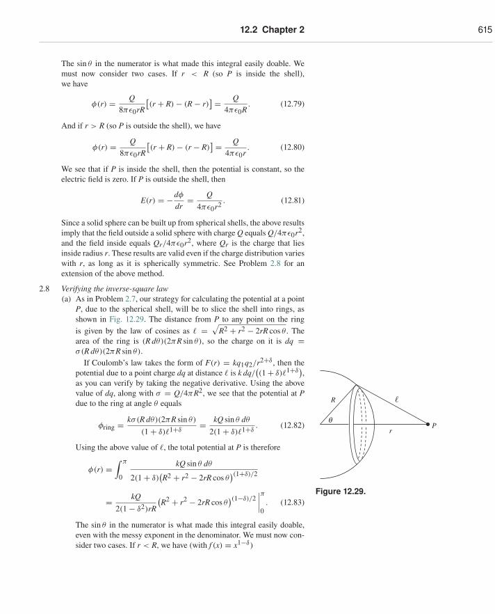
12.2 Chapter 2 615
The sin θ in the numerator is what made this integral easily doable. Wemust now consider two cases. If r < R (so P is inside the shell),we have
φ(r) = Q8πε0rR
[(r + R) − (R − r)
] = Q4πε0R
. (12.79)
And if r > R (so P is outside the shell), we have
φ(r) = Q8πε0rR
[(r + R) − (r − R)
] = Q4πε0r
. (12.80)
We see that if P is inside the shell, then the potential is constant, so theelectric field is zero. If P is outside the shell, then
E(r) = −dφ
dr= Q
4πε0r2 . (12.81)
Since a solid sphere can be built up from spherical shells, the above resultsimply that the field outside a solid sphere with charge Q equals Q/4πε0r2,and the field inside equals Qr/4πε0r2, where Qr is the charge that liesinside radius r. These results are valid even if the charge distribution varieswith r, as long as it is spherically symmetric. See Problem 2.8 for anextension of the above method.
R
rq
P
Figure 12.29.
2.8 Verifying the inverse-square law(a) As in Problem 2.7, our strategy for calculating the potential at a point
P, due to the spherical shell, will be to slice the shell into rings, asshown in Fig. 12.29. The distance from P to any point on the ringis given by the law of cosines as � =
√R2 + r2 − 2rR cos θ . The
area of the ring is (R dθ)(2πR sin θ), so the charge on it is dq =σ(R dθ)(2πR sin θ).
If Coulomb’s law takes the form of F(r) = kq1q2/r2+δ , then thepotential due to a point charge dq at distance � is k dq/
((1+ δ)�1+δ
),
as you can verify by taking the negative derivative. Using the abovevalue of dq, along with σ = Q/4πR2, we see that the potential at Pdue to the ring at angle θ equals
φring = kσ(R dθ)(2πR sin θ)
(1 + δ)�1+δ= kQ sin θ dθ
2(1 + δ)�1+δ. (12.82)
Using the above value of �, the total potential at P is therefore
φ(r) =∫ π
0
kQ sin θ dθ
2(1 + δ)(R2 + r2 − 2rR cos θ
)(1+δ)/2
= kQ2(1 − δ2)rR
(R2 + r2 − 2rR cos θ
)(1−δ)/2∣∣∣∣π0
. (12.83)
The sin θ in the numerator is what made this integral easily doable,even with the messy exponent in the denominator. We must now con-sider two cases. If r < R, we have (with f (x) = x1−δ)
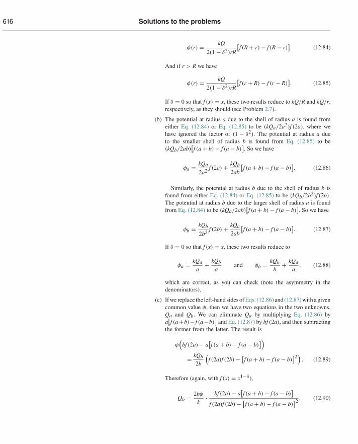
616 Solutions to the problems
φ(r) = kQ2(1 − δ2)rR
[f (R + r) − f (R − r)
]. (12.84)
And if r > R we have
φ(r) = kQ2(1 − δ2)rR
[f (r + R) − f (r − R)
]. (12.85)
If δ = 0 so that f (x) = x, these two results reduce to kQ/R and kQ/r,respectively, as they should (see Problem 2.7).
(b) The potential at radius a due to the shell of radius a is found fromeither Eq. (12.84) or Eq. (12.85) to be (kQa/2a2)f (2a), where wehave ignored the factor of (1 − δ2). The potential at radius a dueto the smaller shell of radius b is found from Eq. (12.85) to be(kQb/2ab)
[f (a + b) − f (a − b)
]. So we have
φa = kQa
2a2 f (2a) + kQb2ab
[f (a + b) − f (a − b)
]. (12.86)
Similarly, the potential at radius b due to the shell of radius b isfound from either Eq. (12.84) or Eq. (12.85) to be (kQb/2b2)f (2b).The potential at radius b due to the larger shell of radius a is foundfrom Eq. (12.84) to be (kQa/2ab)
[f (a + b) − f (a − b)
]. So we have
φb = kQb
2b2 f (2b) + kQa
2ab
[f (a + b) − f (a − b)
]. (12.87)
If δ = 0 so that f (x) = x, these two results reduce to
φa = kQa
a+ kQb
aand φb = kQb
b+ kQa
a, (12.88)
which are correct, as you can check (note the asymmetry in thedenominators).
(c) If we replace the left-hand sides of Eqs. (12.86) and (12.87) with a givencommon value φ, then we have two equations in the two unknowns,Qa and Qb. We can eliminate Qa by multiplying Eq. (12.86) bya[f (a+b)− f (a−b)
]and Eq. (12.87) by bf (2a), and then subtracting
the former from the latter. The result is
φ(
bf (2a) − a[f (a + b) − f (a − b)
])= kQb
2b
(f (2a)f (2b) − [
f (a + b) − f (a − b)]2
). (12.89)
Therefore (again, with f (x) = x1−δ),
Qb = 2bφ
k· bf (2a) − a
[f (a + b) − f (a − b)
]f (2a)f (2b) − [
f (a + b) − f (a − b)]2 . (12.90)
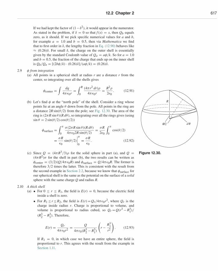
12.2 Chapter 2 617
If we had kept the factor of (1−δ2), it would appear in the numerator.As stated in the problem, if δ = 0 so that f (x) = x, then Qb equalszero, as it should. If we pick specific numerical values for a and b,for example a = 1.0 and b = 0.5, then via Mathematica we findthat to first order in δ, the lengthy fraction in Eq. (12.90) behaves like≈ (0.26)δ. For small δ, the charge on the outer shell is essentiallygiven by the standard Coulomb value of Qa = aφ/k. So for a = 1.0and b = 0.5, the fraction of the charge that ends up on the inner shellis Qb/Qa = [(2bφ/k) · (0.26)δ]/(aφ/k) = (0.26)δ.
2.9 φ from integration(a) All points in a spherical shell at radius r are a distance r from the
center, so integrating over all the shells gives
φcenter =∫
dq4πε0r
=∫ R
0
(4πr2 dr)ρ4πε0r
= R2ρ
2ε0. (12.91)
q/2 dq
R
Figure 12.30.
(b) Let’s find φ at the “north pole” of the shell. Consider a ring whosepoints lie at an angle θ down from the pole. All points in the ring area distance 2R sin(θ/2) from the pole; see Fig. 12.30. The area of thering is (2πR sin θ)(R dθ), so integrating over all the rings gives (usingsin θ = 2 sin(θ/2) cos(θ/2))
φsurface =∫ π
0
σ(2πR sin θ)(R dθ)
4πε02R sin(θ/2)= σR
2ε0
∫ π
0cos(θ/2)
= σRε0
sin(θ/2)
∣∣∣∣π0= σR
ε0. (12.92)
(c) Since Q = (4πR3/3)ρ for the solid sphere in part (a), and Q =(4πR2)σ for the shell in part (b), the two results can be written asφcenter = (3/2)(Q/4πε0R) and φsurface = Q/4πε0R. The former istherefore 3/2 times the latter. This is consistent with the result fromthe second example in Section 2.2, because we know that φsurface forour spherical shell is the same as the potential on the surface of a solidsphere with the same charge Q and radius R.
2.10 A thick shell(a) • For 0 ≤ r ≤ R1, the field is E(r) = 0, because the electric field
inside a shell is zero.
• For R1 ≤ r≤R2, the field is E(r)=Qr/4πε0r2, where Qr is thecharge inside radius r. Charge is proportional to volume, andvolume is proportional to radius cubed, so Qr =Q(r3 −R3
1)/
(R32 − R3
1). Therefore,
E(r) = Qr
4πε0r2 = Q
4πε0(R32 − R3
1)
(r − R3
1r2
). (12.93)
If R1 = 0, in which case we have an entire sphere, the field isproportional to r. This agrees with the result from the example inSection 1.11.
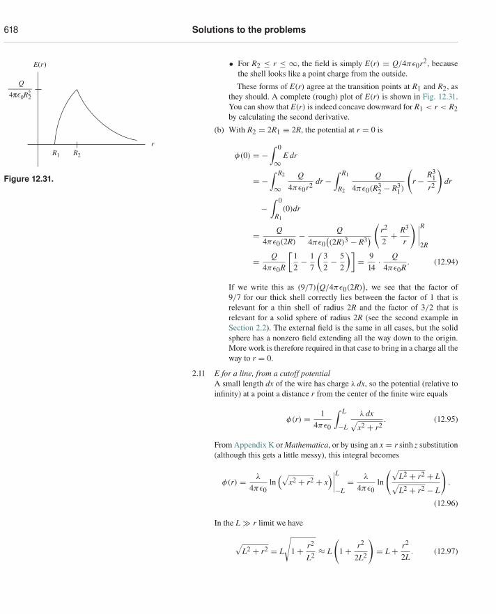
618 Solutions to the problems
• For R2 ≤ r ≤ ∞, the field is simply E(r) = Q/4πε0r2, becausethe shell looks like a point charge from the outside.
These forms of E(r) agree at the transition points at R1 and R2, asthey should. A complete (rough) plot of E(r) is shown in Fig. 12.31.You can show that E(r) is indeed concave downward for R1 < r < R2
r
E(r)
Q
4π 0R22
R1 R2
Figure 12.31.
by calculating the second derivative.
(b) With R2 = 2R1 ≡ 2R, the potential at r = 0 is
φ(0) = −∫ 0
∞E dr
= −∫ R2
∞Q
4πε0r2 dr −∫ R1
R2
Q
4πε0(R32 − R3
1)
(r − R3
1r2
)dr
−∫ 0
R1
(0)dr
= Q4πε0(2R)
− Q4πε0
((2R)3 − R3
)(
r2
2+ R3
r
) ∣∣∣∣R2R
= Q4πε0R
[12− 1
7
(32− 5
2
)]= 9
14· Q
4πε0R. (12.94)
If we write this as (9/7)(Q/4πε0(2R)
), we see that the factor of
9/7 for our thick shell correctly lies between the factor of 1 that isrelevant for a thin shell of radius 2R and the factor of 3/2 that isrelevant for a solid sphere of radius 2R (see the second example inSection 2.2). The external field is the same in all cases, but the solidsphere has a nonzero field extending all the way down to the origin.More work is therefore required in that case to bring in a charge all theway to r = 0.
2.11 E for a line, from a cutoff potentialA small length dx of the wire has charge λ dx, so the potential (relative toinfinity) at a point a distance r from the center of the finite wire equals
φ(r) = 14πε0
∫ L
−L
λ dx√x2 + r2
. (12.95)
From Appendix K or Mathematica, or by using an x = r sinh z substitution(although this gets a little messy), this integral becomes
φ(r) = λ
4πε0ln
(√x2 + r2 + x
)∣∣∣∣L−L= λ
4πε0ln
(√L2 + r2 + L√L2 + r2 − L
).
(12.96)
In the L � r limit we have
√L2 + r2 = L
√1 + r2
L2 ≈ L
(1 + r2
2L2
)= L + r2
2L. (12.97)
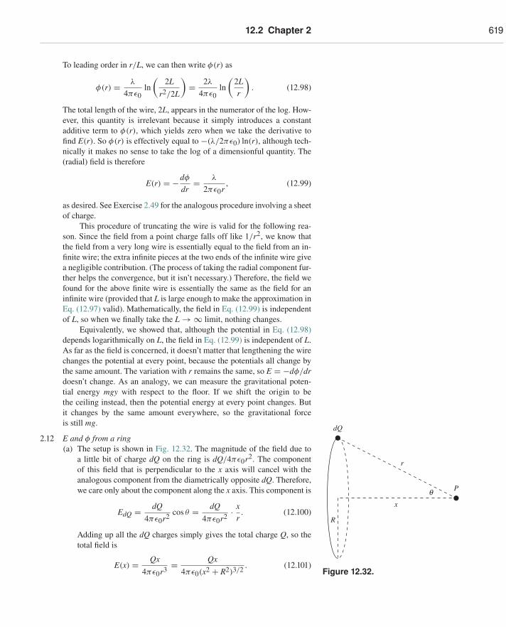
12.2 Chapter 2 619
To leading order in r/L, we can then write φ(r) as
φ(r) = λ
4πε0ln
(2L
r2/2L
)= 2λ
4πε0ln
(2Lr
). (12.98)
The total length of the wire, 2L, appears in the numerator of the log. How-ever, this quantity is irrelevant because it simply introduces a constantadditive term to φ(r), which yields zero when we take the derivative tofind E(r). So φ(r) is effectively equal to −(λ/2πε0) ln(r), although tech-nically it makes no sense to take the log of a dimensionful quantity. The(radial) field is therefore
E(r) = −dφ
dr= λ
2πε0r, (12.99)
as desired. See Exercise 2.49 for the analogous procedure involving a sheetof charge.
This procedure of truncating the wire is valid for the following rea-son. Since the field from a point charge falls off like 1/r2, we know thatthe field from a very long wire is essentially equal to the field from an in-finite wire; the extra infinite pieces at the two ends of the infinite wire givea negligible contribution. (The process of taking the radial component fur-ther helps the convergence, but it isn’t necessary.) Therefore, the field wefound for the above finite wire is essentially the same as the field for aninfinite wire (provided that L is large enough to make the approximation inEq. (12.97) valid). Mathematically, the field in Eq. (12.99) is independentof L, so when we finally take the L → ∞ limit, nothing changes.
Equivalently, we showed that, although the potential in Eq. (12.98)depends logarithmically on L, the field in Eq. (12.99) is independent of L.As far as the field is concerned, it doesn’t matter that lengthening the wirechanges the potential at every point, because the potentials all change bythe same amount. The variation with r remains the same, so E = −dφ/drdoesn’t change. As an analogy, we can measure the gravitational poten-tial energy mgy with respect to the floor. If we shift the origin to bethe ceiling instead, then the potential energy at every point changes. Butit changes by the same amount everywhere, so the gravitational forceis still mg.
R
x
r
dQ
q P
Figure 12.32.
2.12 E and φ from a ring(a) The setup is shown in Fig. 12.32. The magnitude of the field due to
a little bit of charge dQ on the ring is dQ/4πε0r2. The componentof this field that is perpendicular to the x axis will cancel with theanalogous component from the diametrically opposite dQ. Therefore,we care only about the component along the x axis. This component is
EdQ = dQ4πε0r2 cos θ = dQ
4πε0r2 · xr
. (12.100)
Adding up all the dQ charges simply gives the total charge Q, so thetotal field is
E(x) = Qx4πε0r3 = Qx
4πε0(x2 + R2)3/2 . (12.101)
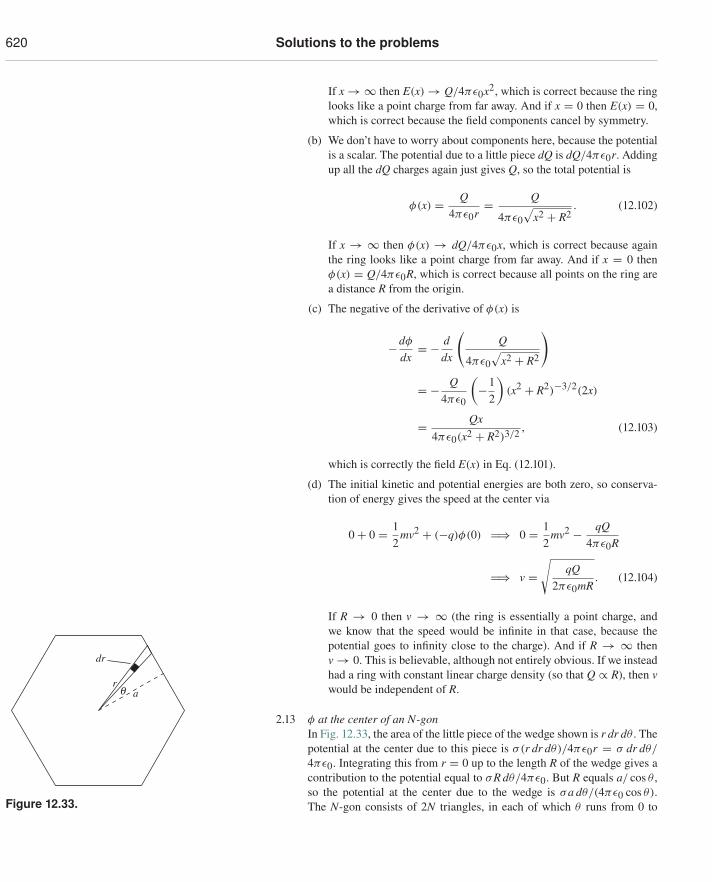
620 Solutions to the problems
If x → ∞ then E(x) → Q/4πε0x2, which is correct because the ringlooks like a point charge from far away. And if x = 0 then E(x) = 0,which is correct because the field components cancel by symmetry.
(b) We don’t have to worry about components here, because the potentialis a scalar. The potential due to a little piece dQ is dQ/4πε0r. Addingup all the dQ charges again just gives Q, so the total potential is
φ(x) = Q4πε0r
= Q
4πε0√
x2 + R2. (12.102)
If x → ∞ then φ(x) → dQ/4πε0x, which is correct because againthe ring looks like a point charge from far away. And if x = 0 thenφ(x) = Q/4πε0R, which is correct because all points on the ring area distance R from the origin.
(c) The negative of the derivative of φ(x) is
−dφ
dx= − d
dx
(Q
4πε0√
x2 + R2
)
= − Q4πε0
(−1
2
)(x2 + R2)−3/2(2x)
= Qx4πε0(x2 + R2)3/2 , (12.103)
which is correctly the field E(x) in Eq. (12.101).
(d) The initial kinetic and potential energies are both zero, so conserva-tion of energy gives the speed at the center via
0 + 0 = 12
mv2 + (−q)φ(0) �⇒ 0 = 12
mv2 − qQ4πε0R
�⇒ v =√
qQ2πε0mR
. (12.104)
If R → 0 then v → ∞ (the ring is essentially a point charge, andwe know that the speed would be infinite in that case, because thepotential goes to infinity close to the charge). And if R → ∞ thenv → 0. This is believable, although not entirely obvious. If we insteadhad a ring with constant linear charge density (so that Q ∝ R), then vwould be independent of R.aq
dr
r
Figure 12.33.
2.13 φ at the center of an N-gonIn Fig. 12.33, the area of the little piece of the wedge shown is r dr dθ . Thepotential at the center due to this piece is σ(r dr dθ)/4πε0r = σ dr dθ/
4πε0. Integrating this from r = 0 up to the length R of the wedge gives acontribution to the potential equal to σR dθ/4πε0. But R equals a/ cos θ ,so the potential at the center due to the wedge is σa dθ/(4πε0 cos θ).The N-gon consists of 2N triangles, in each of which θ runs from 0 to
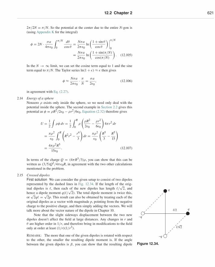
12.2 Chapter 2 621
2π/2N = π/N. So the potential at the center due to the entire N-gon is(using Appendix K for the integral)
φ = 2N · σa4πε0
∫ π/N
0
dθ
cos θ= Nσa
2πε0ln
(1 + sin θ
cos θ
) ∣∣∣∣π/N
0
= Nσa2πε0
ln(
1 + sin(π/N)
cos(π/N)
). (12.105)
In the N → ∞ limit, we can set the cosine term equal to 1 and the sineterm equal to π/N. The Taylor series ln(1 + ε) ≈ ε then gives
φ ≈ Nσa2πε0
· π
N= σa
2ε0, (12.106)
in agreement with Eq. (2.27).
2.14 Energy of a sphereNonzero ρ exists only inside the sphere, so we need only deal with thepotential inside the sphere. The second example in Section 2.2 gives thispotential as φ = ρR2/2ε0 − ρr2/6ε0. Equation (2.32) therefore gives
U = 12
∫ρφ dv = 1
2
∫ R
0ρ
(ρR2
2ε0− ρr2
6ε0
)4πr2 dr
= πρ2
ε0
∫ R
0
(R2r2 − r4
3
)dr = πρ2
ε0
(R5
3− R5
15
)
= 4πρ2R5
15ε0. (12.107)
In terms of the charge Q = (4πR3/3)ρ, you can show that this can bewritten as (3/5)Q2/4πε0R, in agreement with the two other calculationsmentioned in the problem.
2.15 Crossed dipolesFirst solution We can consider the given setup to consist of two dipolesrepresented by the dashed lines in Fig. 12.34. If the length of the orig-
q
q
–q
–q
/2
/ 2
Figure 12.34.
inal dipoles is �, then each of the new dipoles has length �/√
2, andhence a dipole moment q(�/
√2). The total dipole moment is twice this,
or√
2q� = √2p. This result can also be obtained by treating each of the
original dipoles as a vector with magnitude p, pointing from the negativecharge to the positive charge, and then simply adding the vectors. We willtalk more about the vector nature of the dipole in Chapter 10.
Note that the slight sideways displacement between the two newdipoles doesn’t affect the field at large distances. Any changes in r andθ are higher order in 1/r, and therefore bring in modifications to the fieldonly at order at least (1/r)(1/r3).
REMARK: The more that one of the given dipoles is rotated with respectto the other, the smaller the resulting dipole moment is. If the anglebetween the given dipoles is β, you can show that the resulting dipole
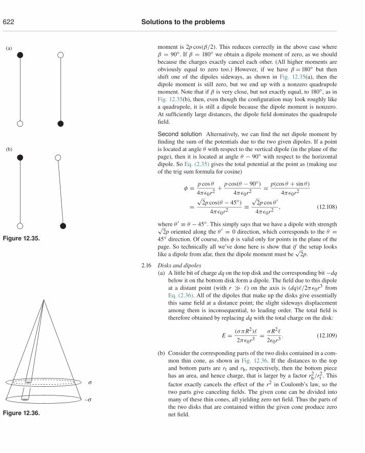
622 Solutions to the problems
moment is 2p cos(β/2). This reduces correctly in the above case whereβ = 90◦. If β = 180◦ we obtain a dipole moment of zero, as we shouldbecause the charges exactly cancel each other. (All higher moments areobviously equal to zero too.) However, if we have β = 180◦ but thenshift one of the dipoles sideways, as shown in Fig. 12.35(a), then the
(a)
(b)
Figure 12.35.
dipole moment is still zero, but we end up with a nonzero quadrupolemoment. Note that if β is very close, but not exactly equal, to 180◦, as inFig. 12.35(b), then, even though the configuration may look roughly likea quadrupole, it is still a dipole because the dipole moment is nonzero.At sufficiently large distances, the dipole field dominates the quadrupolefield.
Second solution Alternatively, we can find the net dipole moment byfinding the sum of the potentials due to the two given dipoles. If a pointis located at angle θ with respect to the vertical dipole (in the plane of thepage), then it is located at angle θ − 90◦ with respect to the horizontaldipole. So Eq. (2.35) gives the total potential at the point as (making useof the trig sum formula for cosine)
φ = p cos θ
4πε0r2 + p cos(θ − 90◦)4πε0r2 = p(cos θ + sin θ)
4πε0r2
=√
2p cos(θ − 45◦)4πε0r2 ≡
√2p cos θ ′4πε0r2 , (12.108)
where θ ′ ≡ θ − 45◦. This simply says that we have a dipole with strength√2p oriented along the θ ′ = 0 direction, which corresponds to the θ =
45◦ direction. Of course, this φ is valid only for points in the plane of thepage. So technically all we’ve done here is show that if the setup lookslike a dipole from afar, then the dipole moment must be
√2p.
2.16 Disks and dipoles(a) A little bit of charge dq on the top disk and the corresponding bit −dq
below it on the bottom disk form a dipole. The field due to this dipoleat a distant point (with r � �) on the axis is (dq)�/2πε0r3 fromEq. (2.36). All of the dipoles that make up the disks give essentiallythis same field at a distance point; the slight sideways displacementamong them is inconsequential, to leading order. The total field is
s
–s
Figure 12.36.
therefore obtained by replacing dq with the total charge on the disk:
E = (σπR2)�
2πε0r3 = σR2�
2ε0r3 . (12.109)
(b) Consider the corresponding parts of the two disks contained in a com-mon thin cone, as shown in Fig. 12.36. If the distances to the topand bottom parts are rt and rb, respectively, then the bottom piecehas an area, and hence charge, that is larger by a factor r2
b/r2t . This
factor exactly cancels the effect of the r2 in Coulomb’s law, so thetwo parts give canceling fields. The given cone can be divided intomany of these thin cones, all yielding zero net field. Thus the parts ofthe two disks that are contained within the given cone produce zeronet field.
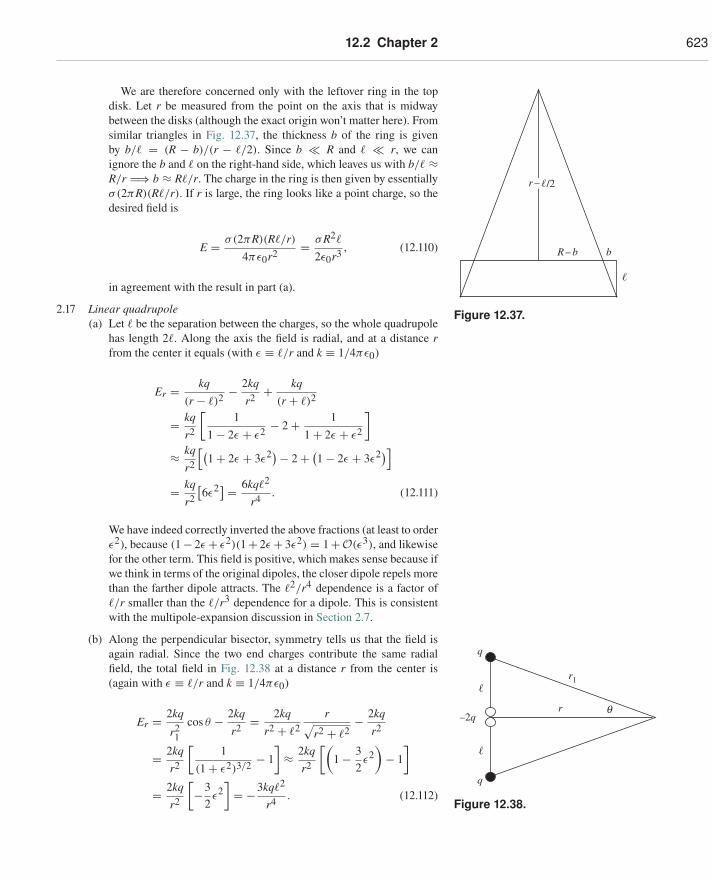
12.2 Chapter 2 623
We are therefore concerned only with the leftover ring in the topdisk. Let r be measured from the point on the axis that is midwaybetween the disks (although the exact origin won’t matter here). Fromsimilar triangles in Fig. 12.37, the thickness b of the ring is given
bR – b
r – /2
Figure 12.37.
by b/� = (R − b)/(r − �/2). Since b � R and � � r, we canignore the b and � on the right-hand side, which leaves us with b/� ≈R/r �⇒ b ≈ R�/r. The charge in the ring is then given by essentiallyσ(2πR)(R�/r). If r is large, the ring looks like a point charge, so thedesired field is
E = σ(2πR)(R�/r)4πε0r2 = σR2�
2ε0r3 , (12.110)
in agreement with the result in part (a).
2.17 Linear quadrupole(a) Let � be the separation between the charges, so the whole quadrupole
has length 2�. Along the axis the field is radial, and at a distance rfrom the center it equals (with ε ≡ �/r and k ≡ 1/4πε0)
Er = kq(r − �)2 − 2kq
r2 + kq(r + �)2
= kqr2
[1
1 − 2ε + ε2 − 2 + 11 + 2ε + ε2
]
≈ kqr2
[(1 + 2ε + 3ε2)− 2 + (
1 − 2ε + 3ε2)]= kq
r2
[6ε2] = 6kq�2
r4 . (12.111)
We have indeed correctly inverted the above fractions (at least to orderε2), because (1− 2ε + ε2)(1+ 2ε + 3ε2) = 1+O(ε3), and likewisefor the other term. This field is positive, which makes sense because ifwe think in terms of the original dipoles, the closer dipole repels morethan the farther dipole attracts. The �2/r4 dependence is a factor of�/r smaller than the �/r3 dependence for a dipole. This is consistentwith the multipole-expansion discussion in Section 2.7.
qr
q
q
–2q
r1
Figure 12.38.
(b) Along the perpendicular bisector, symmetry tells us that the field isagain radial. Since the two end charges contribute the same radialfield, the total field in Fig. 12.38 at a distance r from the center is(again with ε ≡ �/r and k ≡ 1/4πε0)
Er = 2kq
r21
cos θ − 2kqr2 = 2kq
r2 + �2r√
r2 + �2− 2kq
r2
= 2kqr2
[1
(1 + ε2)3/2 − 1]≈ 2kq
r2
[(1 − 3
2ε2
)− 1
]
= 2kqr2
[−3
2ε2
]= −3kq�2
r4 . (12.112)
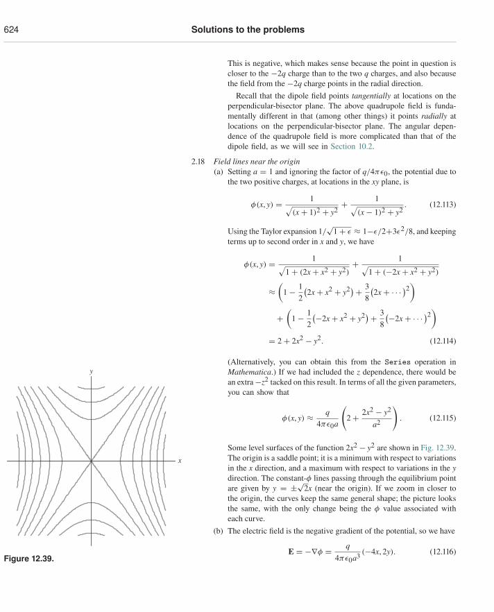
624 Solutions to the problems
This is negative, which makes sense because the point in question iscloser to the −2q charge than to the two q charges, and also becausethe field from the −2q charge points in the radial direction.
Recall that the dipole field points tangentially at locations on theperpendicular-bisector plane. The above quadrupole field is funda-mentally different in that (among other things) it points radially atlocations on the perpendicular-bisector plane. The angular depen-dence of the quadrupole field is more complicated than that of thedipole field, as we will see in Section 10.2.
2.18 Field lines near the origin(a) Setting a = 1 and ignoring the factor of q/4πε0, the potential due to
the two positive charges, at locations in the xy plane, is
φ(x, y) = 1√(x + 1)2 + y2
+ 1√(x − 1)2 + y2
. (12.113)
Using the Taylor expansion 1/√
1 + ε ≈ 1−ε/2+3ε2/8, and keepingterms up to second order in x and y, we have
φ(x, y) = 1√1 + (2x + x2 + y2)
+ 1√1 + (−2x + x2 + y2)
≈(
1 − 12
(2x + x2 + y2)+ 3
8
(2x + · · · )2
)
+(
1 − 12
(−2x + x2 + y2)+ 38
(−2x + · · · )2)
= 2 + 2x2 − y2. (12.114)
(Alternatively, you can obtain this from the Series operation inMathematica.) If we had included the z dependence, there would bean extra −z2 tacked on this result. In terms of all the given parameters,you can show that
φ(x, y) ≈ q4πε0a
(2 + 2x2 − y2
a2
). (12.115)
x
y
Figure 12.39.
Some level surfaces of the function 2x2 − y2 are shown in Fig. 12.39.The origin is a saddle point; it is a minimum with respect to variationsin the x direction, and a maximum with respect to variations in the ydirection. The constant-φ lines passing through the equilibrium pointare given by y = ±√2x (near the origin). If we zoom in closer tothe origin, the curves keep the same general shape; the picture looksthe same, with the only change being the φ value associated witheach curve.
(b) The electric field is the negative gradient of the potential, so we have
E = −∇φ = q4πε0a3 (−4x, 2y). (12.116)
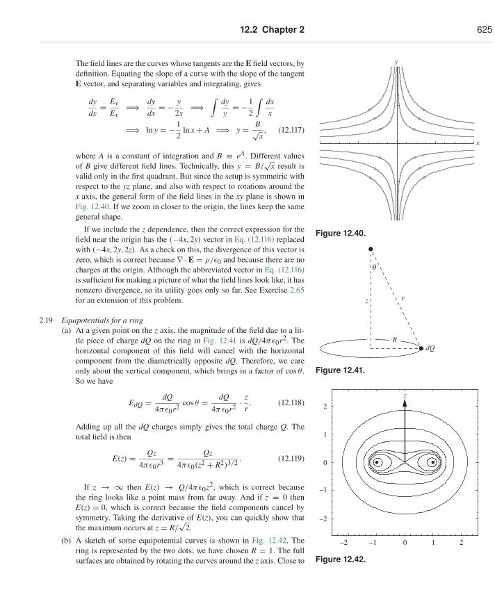
12.2 Chapter 2 625
The field lines are the curves whose tangents are the E field vectors, bydefinition. Equating the slope of a curve with the slope of the tangentE vector, and separating variables and integrating, gives
dydx
= Ey
Ex�⇒ dy
dx= − y
2x�⇒
∫dyy
= −12
∫dxx
�⇒ ln y = −12
ln x + A �⇒ y = B√x
, (12.117)
where A is a constant of integration and B ≡ eA. Different values
x
y
Figure 12.40.
of B give different field lines. Technically, this y = B/√
x result isvalid only in the first quadrant. But since the setup is symmetric withrespect to the yz plane, and also with respect to rotations around thex axis, the general form of the field lines in the xy plane is shown inFig. 12.40. If we zoom in closer to the origin, the lines keep the samegeneral shape.
If we include the z dependence, then the correct expression for thefield near the origin has the (−4x, 2y) vector in Eq. (12.116) replacedwith (−4x, 2y, 2z). As a check on this, the divergence of this vector iszero, which is correct because ∇ ·E = ρ/ε0 and because there are nocharges at the origin. Although the abbreviated vector in Eq. (12.116)is sufficient for making a picture of what the field lines look like, it hasnonzero divergence, so its utility goes only so far. See Exercise 2.65for an extension of this problem. z r
dQ
q
R
Figure 12.41.
2.19 Equipotentials for a ring(a) At a given point on the z axis, the magnitude of the field due to a lit-
tle piece of charge dQ on the ring in Fig. 12.41 is dQ/4πε0r2. Thehorizontal component of this field will cancel with the horizontalcomponent from the diametrically opposite dQ. Therefore, we careonly about the vertical component, which brings in a factor of cos θ .So we have
EdQ = dQ4πε0r2 cos θ = dQ
4πε0r2 · zr
. (12.118)
Adding up all the dQ charges simply gives the total charge Q. The
–1
0 1 2
0
1
2
z
–2
–2 –1
Figure 12.42.
total field is then
E(z) = Qz4πε0r3 = Qz
4πε0(z2 + R2)3/2 . (12.119)
If z → ∞ then E(z) → Q/4πε0z2, which is correct becausethe ring looks like a point mass from far away. And if z = 0 thenE(z) = 0, which is correct because the field components cancel bysymmetry. Taking the derivative of E(z), you can quickly show thatthe maximum occurs at z = R/
√2.
(b) A sketch of some equipotential curves is shown in Fig. 12.42. Thering is represented by the two dots; we have chosen R = 1. The fullsurfaces are obtained by rotating the curves around the z axis. Close to
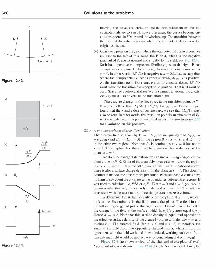
626 Solutions to the problems
the ring, the curves are circles around the dots, which means that theequipotentials are tori in 3D space. Far away, the curves become cir-cles (or spheres in 3D) around the whole setup. The transition betweenE
z
Constant f
x
E
Figure 12.43.
the tori and the spheres occurs where the equipotentials cross at theorigin, as shown.
(c) Consider a point on the z axis where the equipotential curve is concaveup. Just to the left of this point, the E field, which is the negativegradient of φ, points upward and slightly to the right; see Fig. 12.43.So it has a positive x component. Similarly, just to the right, E hasa negative x component. Therefore Ex decreases as x increases acrossx = 0. In other words, ∂Ex/∂x is negative at x = 0. Likewise, at pointswhere the equipotential curve is concave down, ∂Ex/∂x is positive.At the transition point from concave up to concave down, ∂Ex/∂xmust make the transition from negative to positive. That is, it must bezero. Since the equipotential surface is symmetric around the z axis,∂Ey/∂y must also be zero at the transition point.
Ex
f
x
x
x
x
r
s = r0
– r0
___r0 x
r0 x2
r0 2
(Infinite)
–
(a)
(b)
(c)
(d)
–r0
0
2 0
2 0
Figure 12.44.
There are no charges in the free space at the transition point, so ∇ ·E = ρ/ε0 tells us that ∂Ex/∂x+∂Ey/∂y+∂Ez/∂z = 0. Since we justfound that the x and y derivatives are zero, we see that ∂Ez/∂z mustalso be zero. In other words, the transition point is an extremum of Ez,so it coincides with the point we found in part (a). See Exercise 2.66for a variation on this problem.
2.20 A one-dimensional charge distributionThe electric field is given by E = −∇φ, so we quickly find Ex(x) =−ρ0x/ε0 (and Ey = Ez = 0) in the region 0 < x < �, and E = 0in the other two regions. Note that Ex is continuous at x = 0 but not atx = �. This implies that there must be a surface charge density on theplane at x = �.
To obtain the charge distribution, we can use ρ = −ε0∇2φ, or equiv-alently ρ = ε0∇·E. Either of these quickly gives ρ(x) = −ρ0 in the region0 < x < �, and ρ = 0 in the other two regions. But as mentioned above,there is also a surface charge density σ on the plane at x = �. This doesn’tcontradict the volume densities we just found, because those ρ values havenothing to say about the ρ values at the boundaries between the regions. Ifyou tried to calculate −ε0∇2φ or ε0∇ · E at x = 0 and x = �, you wouldobtain results that are, respectively, undefined and infinite. The latter isconsistent with the fact that a surface charge occupies zero volume.
To determine the surface density σ on the plane at x = �, we canlook at the discontinuity in the field across the plane. The field just tothe left is −ρ0�/ε0, and just to the right is zero. Gauss’s law tells us thatthe change in the field at the surface, which is ρ0�/ε0, must equal σ/ε0.Hence σ = ρ0�. Note that this surface density is equal and opposite tothe effective surface density of the charged volume with density −ρ0 andthickness �. The external field (for x < 0 and x > �) is therefore thesame as the field from two oppositely charged sheets, which is zero, inagreement with the field we found above. Indeed, working backward fromthis external field would be another way of concluding that σ = −ρ0�.
Figure 12.44(a) shows a view of the slab and sheet; plots of φ(x),Ex(x), and ρ(x) are shown in Figs. 12.44(b)–(d). As mentioned above, the
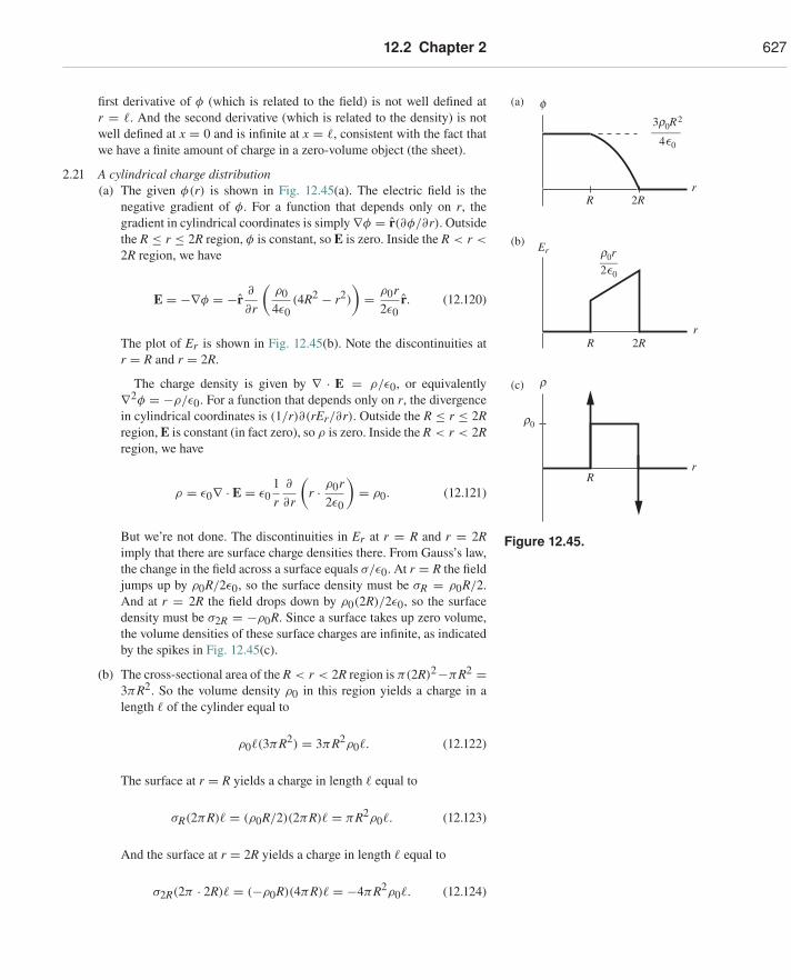
12.2 Chapter 2 627
first derivative of φ (which is related to the field) is not well defined atr = �. And the second derivative (which is related to the density) is notwell defined at x = 0 and is infinite at x = �, consistent with the fact thatwe have a finite amount of charge in a zero-volume object (the sheet).
2.21 A cylindrical charge distribution(a) The given φ(r) is shown in Fig. 12.45(a). The electric field is the
f
Er
r
r0
3r0R2
rR 2R
r
r
R 2R
R
(a)
(b)
(c)
_____
r0r___
4 0
2 0
Figure 12.45.
negative gradient of φ. For a function that depends only on r, thegradient in cylindrical coordinates is simply ∇φ = r(∂φ/∂r). Outsidethe R ≤ r ≤ 2R region, φ is constant, so E is zero. Inside the R < r <
2R region, we have
E = −∇φ = −r∂
∂r
(ρ04ε0
(4R2 − r2)
)= ρ0r
2ε0r. (12.120)
The plot of Er is shown in Fig. 12.45(b). Note the discontinuities atr = R and r = 2R.
The charge density is given by ∇ · E = ρ/ε0, or equivalently∇2φ = −ρ/ε0. For a function that depends only on r, the divergencein cylindrical coordinates is (1/r)∂(rEr/∂r). Outside the R ≤ r ≤ 2Rregion, E is constant (in fact zero), so ρ is zero. Inside the R < r < 2Rregion, we have
ρ = ε0∇ · E = ε01r
∂
∂r
(r · ρ0r
2ε0
)= ρ0. (12.121)
But we’re not done. The discontinuities in Er at r = R and r = 2Rimply that there are surface charge densities there. From Gauss’s law,the change in the field across a surface equals σ/ε0. At r = R the fieldjumps up by ρ0R/2ε0, so the surface density must be σR = ρ0R/2.And at r = 2R the field drops down by ρ0(2R)/2ε0, so the surfacedensity must be σ2R = −ρ0R. Since a surface takes up zero volume,the volume densities of these surface charges are infinite, as indicatedby the spikes in Fig. 12.45(c).
(b) The cross-sectional area of the R < r < 2R region is π(2R)2−πR2 =3πR2. So the volume density ρ0 in this region yields a charge in alength � of the cylinder equal to
ρ0�(3πR2) = 3πR2ρ0�. (12.122)
The surface at r = R yields a charge in length � equal to
σR(2πR)� = (ρ0R/2)(2πR)� = πR2ρ0�. (12.123)
And the surface at r = 2R yields a charge in length � equal to
σ2R(2π · 2R)� = (−ρ0R)(4πR)� = −4πR2ρ0�. (12.124)
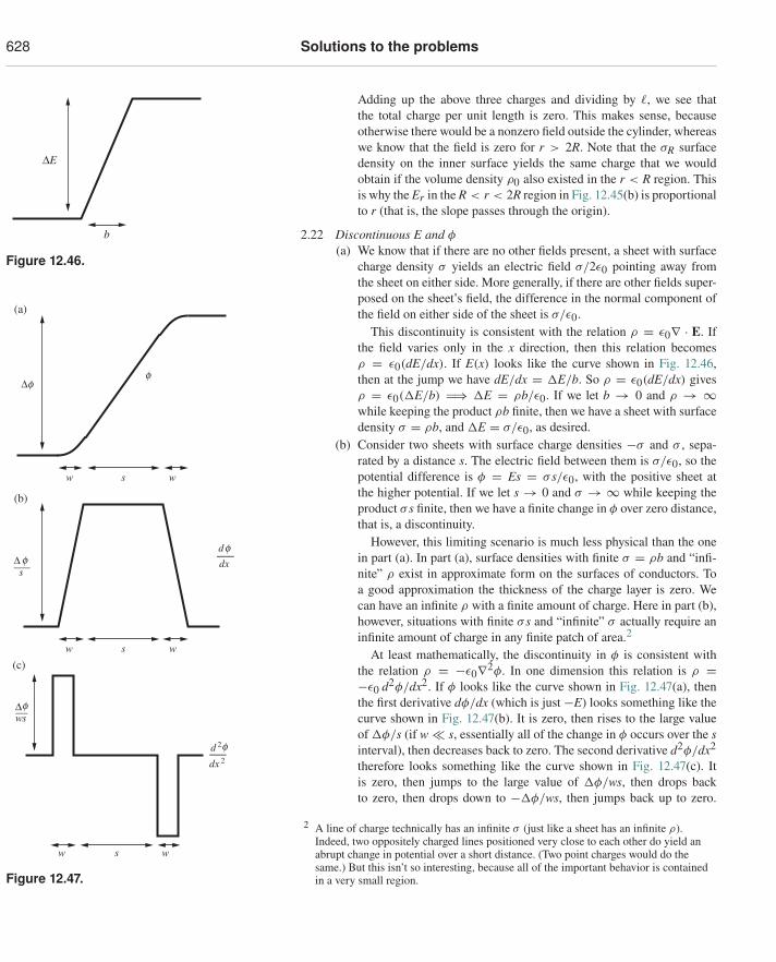
628 Solutions to the problems
Adding up the above three charges and dividing by �, we see thatthe total charge per unit length is zero. This makes sense, becauseotherwise there would be a nonzero field outside the cylinder, whereas
ΔE
b
Figure 12.46.
we know that the field is zero for r > 2R. Note that the σR surfacedensity on the inner surface yields the same charge that we wouldobtain if the volume density ρ0 also existed in the r < R region. Thisis why the Er in the R < r < 2R region in Fig. 12.45(b) is proportionalto r (that is, the slope passes through the origin).
2.22 Discontinuous E and φ
(a) We know that if there are no other fields present, a sheet with surfacecharge density σ yields an electric field σ/2ε0 pointing away fromthe sheet on either side. More generally, if there are other fields super-posed on the sheet’s field, the difference in the normal component ofthe field on either side of the sheet is σ/ε0.
This discontinuity is consistent with the relation ρ = ε0∇ · E. Ifthe field varies only in the x direction, then this relation becomes
Δff
df
sw w
Δs
sw w
sw w
dx
Δws
d 2
dx 2
(a)
(b)
(c)
f
__
__
f
f
Figure 12.47.
ρ = ε0(dE/dx). If E(x) looks like the curve shown in Fig. 12.46,then at the jump we have dE/dx = �E/b. So ρ = ε0(dE/dx) givesρ = ε0(�E/b) �⇒ �E = ρb/ε0. If we let b → 0 and ρ → ∞while keeping the product ρb finite, then we have a sheet with surfacedensity σ = ρb, and �E = σ/ε0, as desired.
(b) Consider two sheets with surface charge densities −σ and σ , sepa-rated by a distance s. The electric field between them is σ/ε0, so thepotential difference is φ = Es = σ s/ε0, with the positive sheet atthe higher potential. If we let s → 0 and σ → ∞ while keeping theproduct σ s finite, then we have a finite change in φ over zero distance,that is, a discontinuity.
However, this limiting scenario is much less physical than the onein part (a). In part (a), surface densities with finite σ = ρb and “infi-nite” ρ exist in approximate form on the surfaces of conductors. Toa good approximation the thickness of the charge layer is zero. Wecan have an infinite ρ with a finite amount of charge. Here in part (b),however, situations with finite σ s and “infinite” σ actually require aninfinite amount of charge in any finite patch of area.2
At least mathematically, the discontinuity in φ is consistent withthe relation ρ = −ε0∇2φ. In one dimension this relation is ρ =−ε0 d2φ/dx2. If φ looks like the curve shown in Fig. 12.47(a), thenthe first derivative dφ/dx (which is just −E) looks something like thecurve shown in Fig. 12.47(b). It is zero, then rises to the large valueof �φ/s (if w � s, essentially all of the change in φ occurs over the sinterval), then decreases back to zero. The second derivative d2φ/dx2
therefore looks something like the curve shown in Fig. 12.47(c). Itis zero, then jumps to the large value of �φ/ws, then drops backto zero, then drops down to −�φ/ws, then jumps back up to zero.
2 A line of charge technically has an infinite σ (just like a sheet has an infinite ρ).Indeed, two oppositely charged lines positioned very close to each other do yield anabrupt change in potential over a short distance. (Two point charges would do thesame.) But this isn’t so interesting, because all of the important behavior is containedin a very small region.
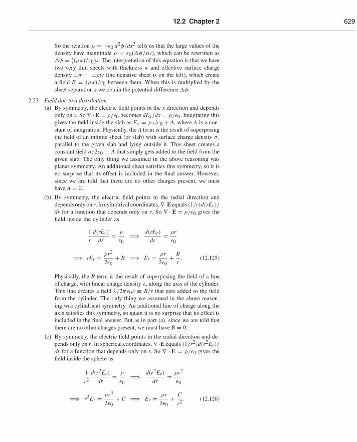
12.2 Chapter 2 629
So the relation ρ = −ε0 d2φ/dx2 tells us that the large values of thedensity have magnitude ρ = ε0(�φ/sw), which can be rewritten as�φ = (
(ρw)/ε0)s. The interpretation of this equation is that we have
two very thin sheets with thickness w and effective surface chargedensity ±σ = ±ρw (the negative sheet is on the left), which createa field E = (ρw)/ε0 between them. When this is multiplied by thesheet separation s we obtain the potential difference �φ.
2.23 Field due to a distribution(a) By symmetry, the electric field points in the x direction and depends
only on x. So ∇ ·E = ρ/ε0 becomes dEx/dx = ρ/ε0. Integrating thisgives the field inside the slab as Ex = ρx/ε0 + A, where A is a con-stant of integration. Physically, the A term is the result of superposingthe field of an infinite sheet (or slab) with surface charge density σ ,parallel to the given slab and lying outside it. This sheet creates aconstant field σ/2ε0 ≡ A that simply gets added to the field from thegiven slab. The only thing we assumed in the above reasoning wasplanar symmetry. An additional sheet satisfies this symmetry, so it isno surprise that its effect is included in the final answer. However,since we are told that there are no other charges present, we musthave A = 0.
(b) By symmetry, the electric field points in the radial direction anddepends only on r. In cylindrical coordinates,∇·E equals (1/r)d(rEr)/dr for a function that depends only on r. So ∇ · E = ρ/ε0 gives thefield inside the cylinder as
1r
d(rEr)
dr= ρ
ε0�⇒ d(rEr)
dr= ρr
ε0
�⇒ rEr = ρr2
2ε0+ B �⇒ Er = ρr
2ε0+ B
r. (12.125)
Physically, the B term is the result of superposing the field of a lineof charge, with linear charge density λ, along the axis of the cylinder.This line creates a field λ/2πε0r ≡ B/r that gets added to the fieldfrom the cylinder. The only thing we assumed in the above reason-ing was cylindrical symmetry. An additional line of charge along theaxis satisfies this symmetry, so again it is no surprise that its effect isincluded in the final answer. But as in part (a), since we are told thatthere are no other charges present, we must have B = 0.
(c) By symmetry, the electric field points in the radial direction and de-pends only on r. In spherical coordinates, ∇·E equals (1/r2)d(r2Er)/dr for a function that depends only on r. So ∇ · E = ρ/ε0 gives thefield inside the sphere as
1r2
d(r2Er)
dr= ρ
ε0�⇒ d(r2Er)
dr= ρr2
ε0
�⇒ r2Er = ρr3
3ε0+ C �⇒ Er = ρr
3ε0+ C
r2 . (12.126)
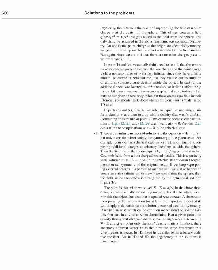
630 Solutions to the problems
Physically, the C term is the result of superposing the field of a pointcharge q at the center of the sphere. This charge creates a fieldq/4πε0r2 ≡ C/r2 that gets added to the field from the sphere. Theonly thing we assumed in the above reasoning was spherical symme-try. An additional point charge at the origin satisfies this symmetry,so again it is no surprise that its effect is included in the final answer.But again, since we are told that there are no other charges present,we must have C = 0.
In parts (b) and (c), we actually didn’t need to be told that there wereno other charges present, because the line charge and the point chargeyield a nonzero value of ρ (in fact infinite, since they have a finiteamount of charge in zero volume), so they violate our assumptionof uniform volume charge density inside the object. In part (a) theadditional sheet was located outside the slab, so it didn’t affect the ρ
inside. Of course, we could superpose a spherical or cylindrical shelloutside our given sphere or cylinder, but these create zero field in theirinteriors. You should think about what is different about a “ball” in the1D case.
In parts (b) and (c), how did we solve an equation involving a uni-form density ρ and then end up with a density that wasn’t uniform(containing an extra line or point)? This occurred because our calcula-tions in Eqs. (12.125) and (12.126) aren’t valid at r = 0. Problem 2.26deals with the complications at r = 0 in the spherical case.
(d) There are an infinite number of solutions to the equation ∇·E = ρ/ε0,but only a certain subset satisfy the symmetry of the given setup. Forexample, consider the spherical case in part (c), and imagine super-posing additional charges at arbitrary locations outside the sphere.Then the field inside the sphere equals Er = ρr/3ε0 plus the standardCoulomb fields from all the charges located outside. This is a perfectlyvalid solution to ∇ · E = ρ/ε0 in the interior. But it doesn’t respectthe spherical symmetry of the original setup. If we keep superpos-ing external charges in a particular manner until we just so happen tocreate an entire infinite uniform cylinder containing the sphere, thenthe field inside the sphere is now given by the cylindrical solutionin part (b).
The point is that when we solved ∇ · E = ρ/ε0 in the above threecases, we were actually demanding not only that the density equaledρ inside the object, but also that it equaled zero outside. A shortcut toincorporating this information (or at least the important aspect of it)was simply to demand that the solution possessed a certain symmetry.If we had an unsymmetrical object, then we wouldn’t be able to takethis shortcut. In any case, when determining E at a given point, thedensity throughout all space matters, even though when determining∇ · E at a given point only the local density matters. In short, thereare many different vector fields that have the same divergence in agiven region in space. In 1D, these fields differ by an arbitrary addi-tive constant. But in 2D and 3D, the degeneracy in the solutions ismuch larger.
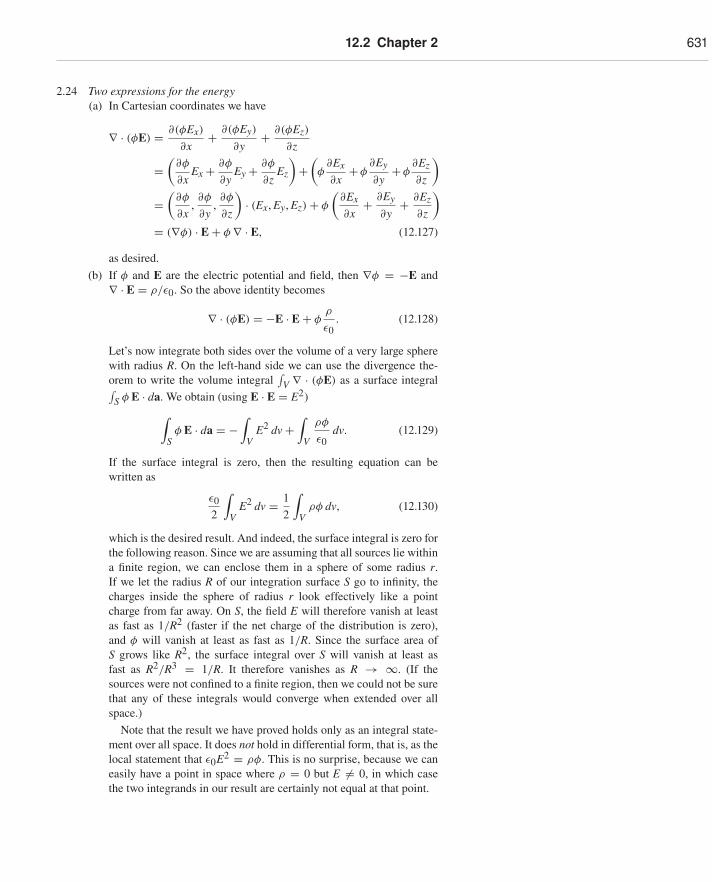
12.2 Chapter 2 631
2.24 Two expressions for the energy(a) In Cartesian coordinates we have
∇ · (φE) = ∂(φEx)
∂x+ ∂(φEy)
∂y+ ∂(φEz)
∂z
=(
∂φ
∂xEx + ∂φ
∂yEy + ∂φ
∂zEz
)+
(φ
∂Ex
∂x+φ
∂Ey
∂y+φ
∂Ez
∂z
)
=(
∂φ
∂x,∂φ
∂y,∂φ
∂z
)· (Ex, Ey, Ez) + φ
(∂Ex
∂x+ ∂Ey
∂y+ ∂Ez
∂z
)= (∇φ) · E + φ ∇ · E, (12.127)
as desired.(b) If φ and E are the electric potential and field, then ∇φ = −E and
∇ · E = ρ/ε0. So the above identity becomes
∇ · (φE) = −E · E + φρ
ε0. (12.128)
Let’s now integrate both sides over the volume of a very large spherewith radius R. On the left-hand side we can use the divergence the-orem to write the volume integral
∫V ∇ · (φE) as a surface integral∫
S φ E · da. We obtain (using E · E = E2)∫Sφ E · da = −
∫V
E2 dv +∫
V
ρφ
ε0dv. (12.129)
If the surface integral is zero, then the resulting equation can bewritten as
ε02
∫V
E2 dv = 12
∫V
ρφ dv, (12.130)
which is the desired result. And indeed, the surface integral is zero forthe following reason. Since we are assuming that all sources lie withina finite region, we can enclose them in a sphere of some radius r.If we let the radius R of our integration surface S go to infinity, thecharges inside the sphere of radius r look effectively like a pointcharge from far away. On S, the field E will therefore vanish at leastas fast as 1/R2 (faster if the net charge of the distribution is zero),and φ will vanish at least as fast as 1/R. Since the surface area ofS grows like R2, the surface integral over S will vanish at least asfast as R2/R3 = 1/R. It therefore vanishes as R → ∞. (If thesources were not confined to a finite region, then we could not be surethat any of these integrals would converge when extended over allspace.)
Note that the result we have proved holds only as an integral state-ment over all space. It does not hold in differential form, that is, as thelocal statement that ε0E2 = ρφ. This is no surprise, because we caneasily have a point in space where ρ = 0 but E �= 0, in which casethe two integrands in our result are certainly not equal at that point.
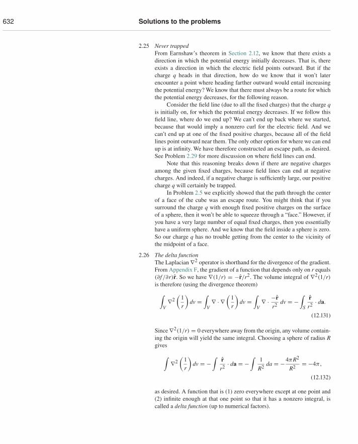
632 Solutions to the problems
2.25 Never trappedFrom Earnshaw’s theorem in Section 2.12, we know that there exists adirection in which the potential energy initially decreases. That is, thereexists a direction in which the electric field points outward. But if thecharge q heads in that direction, how do we know that it won’t laterencounter a point where heading farther outward would entail increasingthe potential energy? We know that there must always be a route for whichthe potential energy decreases, for the following reason.
Consider the field line (due to all the fixed charges) that the charge qis initially on, for which the potential energy decreases. If we follow thisfield line, where do we end up? We can’t end up back where we started,because that would imply a nonzero curl for the electric field. And wecan’t end up at one of the fixed positive charges, because all of the fieldlines point outward near them. The only other option for where we can endup is at infinity. We have therefore constructed an escape path, as desired.See Problem 2.29 for more discussion on where field lines can end.
Note that this reasoning breaks down if there are negative chargesamong the given fixed charges, because field lines can end at negativecharges. And indeed, if a negative charge is sufficiently large, our positivecharge q will certainly be trapped.
In Problem 2.5 we explicitly showed that the path through the centerof a face of the cube was an escape route. You might think that if yousurround the charge q with enough fixed positive charges on the surfaceof a sphere, then it won’t be able to squeeze through a “face.” However, ifyou have a very large number of equal fixed charges, then you essentiallyhave a uniform sphere. And we know that the field inside a sphere is zero.So our charge q has no trouble getting from the center to the vicinity ofthe midpoint of a face.
2.26 The delta functionThe Laplacian ∇2 operator is shorthand for the divergence of the gradient.From Appendix F, the gradient of a function that depends only on r equals(∂f /∂r)r. So we have ∇(1/r) = −r/r2. The volume integral of ∇2(1/r)is therefore (using the divergence theorem)∫
V∇2
(1r
)dv =
∫V∇ · ∇
(1r
)dv =
∫V∇ · −r
r2 dv = −∫
S
rr2 · da.
(12.131)
Since ∇2(1/r) = 0 everywhere away from the origin, any volume contain-ing the origin will yield the same integral. Choosing a sphere of radius Rgives
∫∇2
(1r
)dv = −
∫rr2 · da = −
∫1
R2 da = −4πR2
R2 = −4π ,
(12.132)
as desired. A function that is (1) zero everywhere except at one point and(2) infinite enough at that one point so that it has a nonzero integral, iscalled a delta function (up to numerical factors).
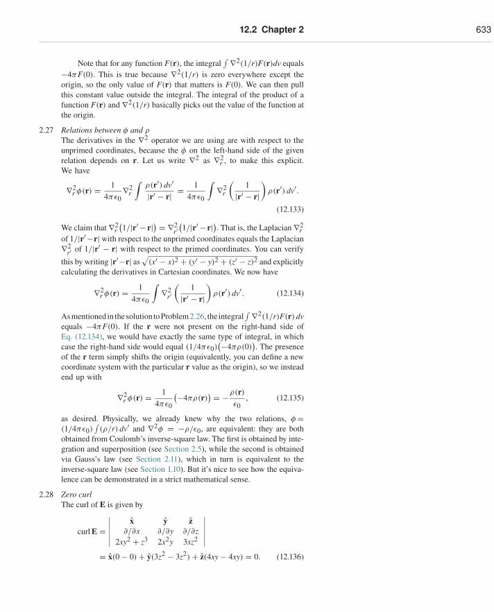
12.2 Chapter 2 633
Note that for any function F(r), the integral∫ ∇2(1/r)F(r)dv equals
−4πF(0). This is true because ∇2(1/r) is zero everywhere except theorigin, so the only value of F(r) that matters is F(0). We can then pullthis constant value outside the integral. The integral of the product of afunction F(r) and ∇2(1/r) basically picks out the value of the function atthe origin.
2.27 Relations between φ and ρ
The derivatives in the ∇2 operator we are using are with respect to theunprimed coordinates, because the φ on the left-hand side of the givenrelation depends on r. Let us write ∇2 as ∇2
r , to make this explicit.We have
∇2r φ(r) = 1
4πε0∇2
r
∫ρ(r′) dv′|r′ − r| = 1
4πε0
∫∇2
r
(1
|r′ − r|)
ρ(r′) dv′.
(12.133)
We claim that ∇2r(1/|r′ −r|) = ∇2
r′(1/|r′ −r|). That is, the Laplacian ∇2
rof 1/|r′−r| with respect to the unprimed coordinates equals the Laplacian∇2
r′ of 1/|r′ − r| with respect to the primed coordinates. You can verify
this by writing |r′−r| as√
(x′ − x)2 + (y′ − y)2 + (z′ − z)2 and explicitlycalculating the derivatives in Cartesian coordinates. We now have
∇2r φ(r) = 1
4πε0
∫∇2
r′(
1|r′ − r|
)ρ(r′) dv′. (12.134)
Asmentioned in thesolution toProblem2.26, the integral∫ ∇2(1/r)F(r) dv
equals −4πF(0). If the r were not present on the right-hand side ofEq. (12.134), we would have exactly the same type of integral, in whichcase the right-hand side would equal (1/4πε0)
(−4πρ(0)). The presence
of the r term simply shifts the origin (equivalently, you can define a newcoordinate system with the particular r value as the origin), so we insteadend up with
∇2r φ(r) = 1
4πε0
(−4πρ(r)) = −ρ(r)
ε0, (12.135)
as desired. Physically, we already knew why the two relations, φ =(1/4πε0)
∫(ρ/r) dv′ and ∇2φ = −ρ/ε0, are equivalent: they are both
obtained from Coulomb’s inverse-square law. The first is obtained by inte-gration and superposition (see Section 2.5), while the second is obtainedvia Gauss’s law (see Section 2.11), which in turn is equivalent to theinverse-square law (see Section 1.10). But it’s nice to see how the equiva-lence can be demonstrated in a strict mathematical sense.
2.28 Zero curlThe curl of E is given by
curl E =∣∣∣∣∣∣
x y z∂/∂x ∂/∂y ∂/∂z
2xy2 + z3 2x2y 3xz2
∣∣∣∣∣∣= x(0 − 0) + y(3z2 − 3z2) + z(4xy − 4xy) = 0. (12.136)
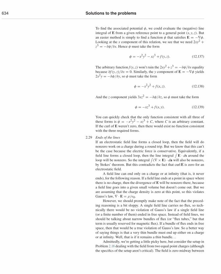
634 Solutions to the problems
To find the associated potential φ, we could evaluate the (negative) lineintegral of E from a given reference point to a general point (x, y, z). Butan easier method is simply to find a function φ that satisfies E = −∇φ.Looking at the x component of this relation, we see that we need 2xy2 +z3 = −∂φ/∂x. Hence φ must take the form
φ = −x2y2 − xz3 + f (y, z). (12.137)
The arbitrary function f (y, z) won’t ruin the 2xy2+ z3 = −∂φ/∂x equalitybecause ∂f (y, z)/∂x = 0. Similarly, the y component of E = −∇φ yields2x2y = −∂φ/∂y, so φ must take the form
φ = −x2y2 + f (x, z). (12.138)
And the z component yields 3xz2 = −∂φ/∂z, so φ must take the form
φ = −xz3 + f (x, y). (12.139)
You can quickly check that the only function consistent with all three ofthese forms is φ = −x2y2 − xz3 + C, where C is an arbitrary constant.If the curl of E weren’t zero, then there would exist no function consistentwith the three required forms.
2.29 Ends of the linesIf an electrostatic field line forms a closed loop, then the field will dononzero work on a charge during a round trip. But we know that this can’tbe the case because the electric force is conservative. Equivalently, if afield line forms a closed loop, then the line integral
∫E · ds around the
loop will be nonzero. So the integral∫(∇ × E) · da will also be nonzero,
by Stokes’ theorem. But this contradicts the fact that curl E is zero for anelectrostatic field.
A field line can end only on a charge or at infinity (that is, it neverends), for the following reason. If a field line ends at a point in space wherethere is no charge, then the divergence of E will be nonzero there, becausea field line goes into a given small volume but doesn’t come out. But weare assuming that the charge density is zero at this point, so this violatesGauss’s law, ∇ · E = ρ/ε0.
However, we should promptly make note of the fact that the preced-ing reasoning is a bit sloppy. A single field line carries no flux, so tech-nically there would be no violation of Gauss’s law if a single field line(or a finite number of them) ended in free space. Instead of field lines, weshould be talking about narrow bundles of flux (or “flux tubes,” but thatterm is usually reserved for magnetic flux). If a bundle of flux ends in freespace, then that would be a true violation of Gauss’s law. So a better wayof saying things is that a very thin bundle must end up either on a chargeor at infinity. Well, that is if it remains a thin bundle. . .
Admittedly, we’re getting a little picky here, but consider the setup inProblem 2.18 dealing with the field from two equal point charges (althoughthe specifics of the setup aren’t critical). The field is zero midway between
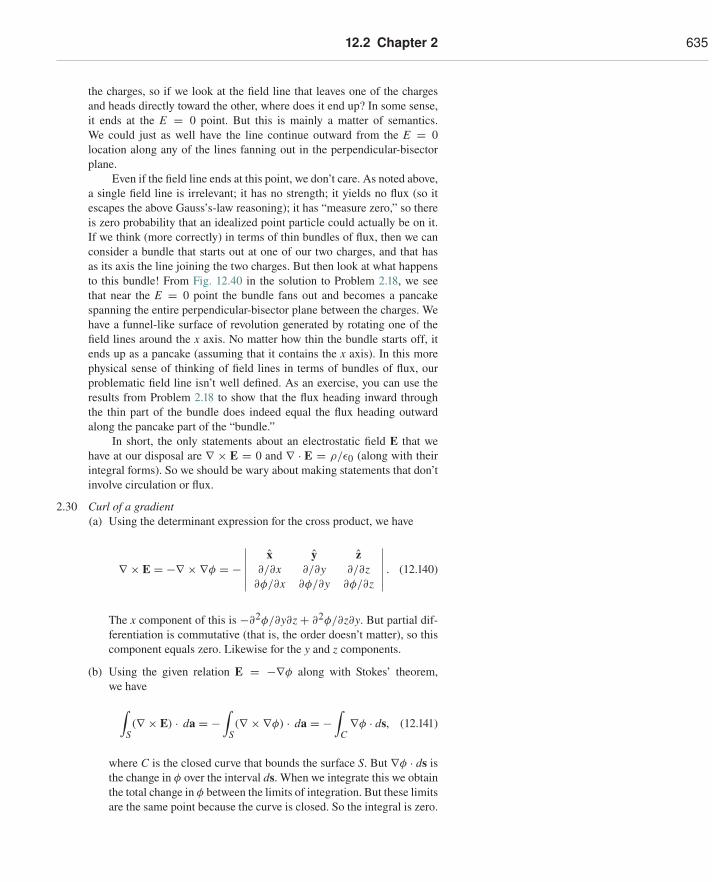
12.2 Chapter 2 635
the charges, so if we look at the field line that leaves one of the chargesand heads directly toward the other, where does it end up? In some sense,it ends at the E = 0 point. But this is mainly a matter of semantics.We could just as well have the line continue outward from the E = 0location along any of the lines fanning out in the perpendicular-bisectorplane.
Even if the field line ends at this point, we don’t care. As noted above,a single field line is irrelevant; it has no strength; it yields no flux (so itescapes the above Gauss’s-law reasoning); it has “measure zero,” so thereis zero probability that an idealized point particle could actually be on it.If we think (more correctly) in terms of thin bundles of flux, then we canconsider a bundle that starts out at one of our two charges, and that hasas its axis the line joining the two charges. But then look at what happensto this bundle! From Fig. 12.40 in the solution to Problem 2.18, we seethat near the E = 0 point the bundle fans out and becomes a pancakespanning the entire perpendicular-bisector plane between the charges. Wehave a funnel-like surface of revolution generated by rotating one of thefield lines around the x axis. No matter how thin the bundle starts off, itends up as a pancake (assuming that it contains the x axis). In this morephysical sense of thinking of field lines in terms of bundles of flux, ourproblematic field line isn’t well defined. As an exercise, you can use theresults from Problem 2.18 to show that the flux heading inward throughthe thin part of the bundle does indeed equal the flux heading outwardalong the pancake part of the “bundle.”
In short, the only statements about an electrostatic field E that wehave at our disposal are ∇ × E = 0 and ∇ · E = ρ/ε0 (along with theirintegral forms). So we should be wary about making statements that don’tinvolve circulation or flux.
2.30 Curl of a gradient(a) Using the determinant expression for the cross product, we have
∇ × E = −∇ × ∇φ = −∣∣∣∣∣∣
x y z∂/∂x ∂/∂y ∂/∂z
∂φ/∂x ∂φ/∂y ∂φ/∂z
∣∣∣∣∣∣ . (12.140)
The x component of this is −∂2φ/∂y∂z + ∂2φ/∂z∂y. But partial dif-ferentiation is commutative (that is, the order doesn’t matter), so thiscomponent equals zero. Likewise for the y and z components.
(b) Using the given relation E = −∇φ along with Stokes’ theorem,we have
∫S(∇ × E) · da = −
∫S(∇ × ∇φ) · da = −
∫C∇φ · ds, (12.141)
where C is the closed curve that bounds the surface S. But ∇φ · ds isthe change in φ over the interval ds. When we integrate this we obtainthe total change in φ between the limits of integration. But these limitsare the same point because the curve is closed. So the integral is zero.
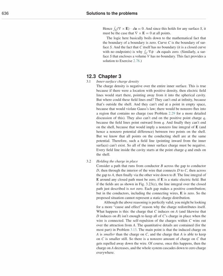
636 Solutions to the problems
Hence∫
S(∇ × E) · da = 0. And since this holds for any surface S, itmust be the case that ∇ × E = 0 at all points.
The logic here basically boils down to the mathematical fact thatthe boundary of a boundary is zero. Curve C is the boundary of sur-face S. And the fact that C itself has no boundary (it is a closed curvewith no endpoints) is why
∫C ∇φ · ds equals zero. (Similarly, a sur-
face S that encloses a volume V has no boundary. This fact provides asolution to Exercise 2.78.)
12.3 Chapter 33.1 Inner-surface charge density
The charge density is negative over the entire inner surface. This is truebecause if there were a location with positive density, then electric fieldlines would start there, pointing away from it into the spherical cavity.But where could these field lines end? They can’t end at infinity, becausethat’s outside the shell. And they can’t end at a point in empty space,because that would violate Gauss’s law; there would be nonzero flux intoa region that contains no charge (see Problem 2.29 for a more detaileddiscussion of this). They also can’t end on the positive point charge q,because the field lines point outward from q. And finally they can’t endon the shell, because that would imply a nonzero line integral of E (andhence a nonzero potential difference) between two points on the shell.But we know that all points on the conducting shell are at the samepotential. Therefore, such a field line (pointing inward from the innersurface) can’t exist. So all of the inner surface charge must be negative.Every field line inside the cavity starts at the point charge q and ends onthe shell.
3.2 Holding the charge in placeConsider a path that runs from conductor B across the gap to conductorD, then through the interior of the wire that connects D to C, then acrossthe gap to A, then finally via the other wire down to B. The line integral ofE around any closed path must be zero, if E is a static electric field. Butif the fields are as shown in Fig. 3.23(c), the line integral over the closedpath just described is not zero. Each gap makes a positive contribution;but in the conductors, including the connecting wires, E is zero. So theproposed situation cannot represent a static charge distribution.
Although the above reasoning is perfectly valid, you might be lookingfor a more “cause and effect” reason why the charge redistributes itself.What happens is this: the charge that C induces on A (and likewise thatD induces on B) isn’t enough to keep all of C’s charge in place when thewire is connected. The self-repulsion of the charges within C wins outover the attraction from A. The quantitative details are contained (for themost part) in Problem 3.13. The main point is that the induced charge onA is smaller than the charge on C, and the charge that A is able to keepon C is smaller still. So there is a nonzero amount of charge on C thatgets repelled away down the wire. Of course, once this happens, then thecharge on A decreases, and the whole system cascades down to zero chargeeverywhere.
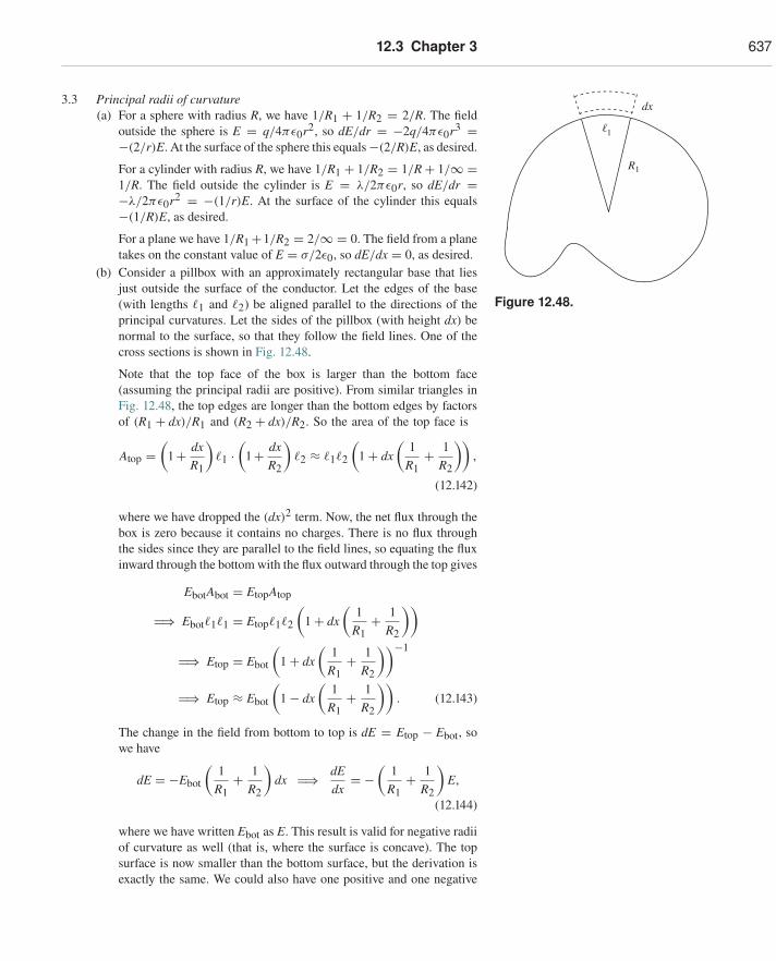
12.3 Chapter 3 637
3.3 Principal radii of curvature(a) For a sphere with radius R, we have 1/R1 + 1/R2 = 2/R. The field
outside the sphere is E = q/4πε0r2, so dE/dr = −2q/4πε0r3 =−(2/r)E. At the surface of the sphere this equals−(2/R)E, as desired.
For a cylinder with radius R, we have 1/R1 + 1/R2 = 1/R + 1/∞ =1/R. The field outside the cylinder is E = λ/2πε0r, so dE/dr =−λ/2πε0r2 = −(1/r)E. At the surface of the cylinder this equals−(1/R)E, as desired.
For a plane we have 1/R1+1/R2 = 2/∞ = 0. The field from a planetakes on the constant value of E = σ/2ε0, so dE/dx = 0, as desired.
(b) Consider a pillbox with an approximately rectangular base that liesjust outside the surface of the conductor. Let the edges of the base(with lengths �1 and �2) be aligned parallel to the directions of theprincipal curvatures. Let the sides of the pillbox (with height dx) benormal to the surface, so that they follow the field lines. One of thecross sections is shown in Fig. 12.48.
R1
1
dx
Figure 12.48.
Note that the top face of the box is larger than the bottom face(assuming the principal radii are positive). From similar triangles inFig. 12.48, the top edges are longer than the bottom edges by factorsof (R1 + dx)/R1 and (R2 + dx)/R2. So the area of the top face is
Atop =(
1+ dxR1
)�1 ·
(1+ dx
R2
)�2 ≈ �1�2
(1 + dx
(1
R1+ 1
R2
)),
(12.142)
where we have dropped the (dx)2 term. Now, the net flux through thebox is zero because it contains no charges. There is no flux throughthe sides since they are parallel to the field lines, so equating the fluxinward through the bottom with the flux outward through the top gives
EbotAbot = EtopAtop
�⇒ Ebot�1�1 = Etop�1�2
(1 + dx
(1
R1+ 1
R2
))
�⇒ Etop = Ebot
(1 + dx
(1
R1+ 1
R2
))−1
�⇒ Etop ≈ Ebot
(1 − dx
(1
R1+ 1
R2
)). (12.143)
The change in the field from bottom to top is dE = Etop − Ebot, sowe have
dE = −Ebot
(1
R1+ 1
R2
)dx �⇒ dE
dx= −
(1
R1+ 1
R2
)E,
(12.144)
where we have written Ebot as E. This result is valid for negative radiiof curvature as well (that is, where the surface is concave). The topsurface is now smaller than the bottom surface, but the derivation isexactly the same. We could also have one positive and one negative
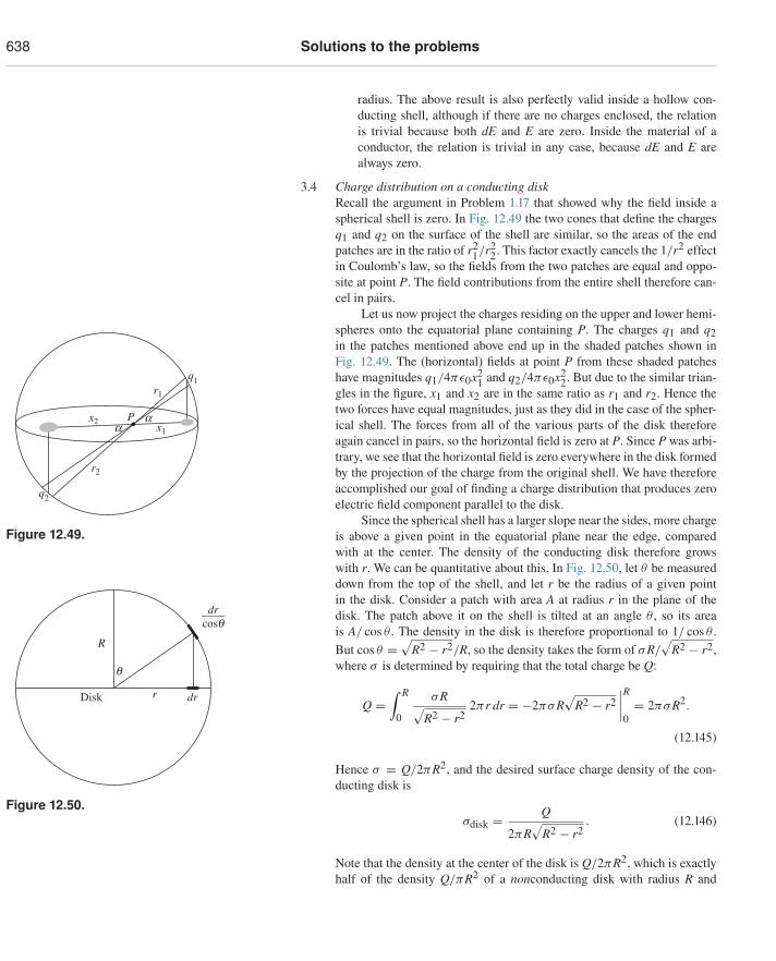
638 Solutions to the problems
radius. The above result is also perfectly valid inside a hollow con-ducting shell, although if there are no charges enclosed, the relationis trivial because both dE and E are zero. Inside the material of aconductor, the relation is trivial in any case, because dE and E arealways zero.
3.4 Charge distribution on a conducting diskRecall the argument in Problem 1.17 that showed why the field inside aspherical shell is zero. In Fig. 12.49 the two cones that define the charges
P
q1
q2
r2
x2
r1
x1aa
Figure 12.49.
q1 and q2 on the surface of the shell are similar, so the areas of the endpatches are in the ratio of r2
1/r22. This factor exactly cancels the 1/r2 effect
in Coulomb’s law, so the fields from the two patches are equal and oppo-site at point P. The field contributions from the entire shell therefore can-cel in pairs.
Let us now project the charges residing on the upper and lower hemi-spheres onto the equatorial plane containing P. The charges q1 and q2in the patches mentioned above end up in the shaded patches shown inFig. 12.49. The (horizontal) fields at point P from these shaded patcheshave magnitudes q1/4πε0x2
1 and q2/4πε0x22. But due to the similar trian-
gles in the figure, x1 and x2 are in the same ratio as r1 and r2. Hence thetwo forces have equal magnitudes, just as they did in the case of the spher-ical shell. The forces from all of the various parts of the disk thereforeagain cancel in pairs, so the horizontal field is zero at P. Since P was arbi-trary, we see that the horizontal field is zero everywhere in the disk formedby the projection of the charge from the original shell. We have thereforeaccomplished our goal of finding a charge distribution that produces zeroelectric field component parallel to the disk.
Since the spherical shell has a larger slope near the sides, more chargeis above a given point in the equatorial plane near the edge, comparedwith at the center. The density of the conducting disk therefore growswith r. We can be quantitative about this. In Fig. 12.50, let θ be measured
Disk
q
r dr
dr
R
cosq
Figure 12.50.
down from the top of the shell, and let r be the radius of a given pointin the disk. Consider a patch with area A at radius r in the plane of thedisk. The patch above it on the shell is tilted at an angle θ , so its areais A/ cos θ . The density in the disk is therefore proportional to 1/ cos θ .But cos θ =
√R2 − r2/R, so the density takes the form of σR/
√R2 − r2,
where σ is determined by requiring that the total charge be Q:
Q =∫ R
0
σR√R2 − r2
2πr dr = −2πσR√
R2 − r2∣∣∣∣R0= 2πσR2.
(12.145)
Hence σ = Q/2πR2, and the desired surface charge density of the con-ducting disk is
σdisk = Q
2πR√
R2 − r2. (12.146)
Note that the density at the center of the disk is Q/2πR2, which is exactlyhalf of the density Q/πR2 of a nonconducting disk with radius R and
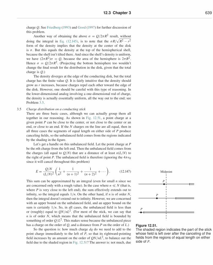
12.3 Chapter 3 639
charge Q. See Friedberg (1993) and Good (1997) for further discussion ofthis problem.
Another way of obtaining the above σ = Q/2πR2 result, withoutdoing the integral in Eq. (12.145), is to note that the σR/
√R2 − r2
form of the density implies that the density at the center of the diskis σ . But this equals the density at the top of the hemispherical shell,because the shell isn’t tilted there. And since the shell’s density is uniform,we have (2πR2)σ = Q, because the area of the hemisphere is 2πR2.Hence σ = Q/2πR2. (Projecting the bottom hemisphere too wouldn’tchange the final result for the distribution in the disk, given that the totalcharge is Q.)
The density diverges at the edge of the conducting disk, but the totalcharge has the finite value Q. It is fairly intuitive that the density shouldgrow as r increases, because charges repel each other toward the edge ofthe disk. However, one should be careful with this type of reasoning. Inthe lower-dimensional analog involving a one-dimensional rod of charge,the density is actually essentially uniform, all the way out to the end; seeProblem 3.5.
3.5 Charge distribution on a conducting stickThere are three basic cases, although we can actually group them alltogether in our reasoning. As shown in Fig. 12.51, a point charge at a
P
P
P
Midpoint
Figure 12.51.The shaded region indicates the part of the stickwhose field is left over after the canceling of thefields from the regions of equal length on eitherside of P.
given point P can be close to the center, or not close to the center or anend, or close to an end. If the N charges on the line are all equal, then inall three cases the segments of equal length on either side of P producecanceling fields, so the unbalanced field comes from the regions indicatedby the shading in the figure.
Let’s get a handle on this unbalanced field. Let the point charge at Pbe the nth charge from the left end. Then the unbalanced field comes fromthe charges (all equal to Q/N) that are a distance of at least n(L/N) tothe right of point P. The unbalanced field is therefore (ignoring the 4πε0since it will cancel throughout this problem)
E = Q/N(L/N)2
(1n2 + 1
(n + 1)2 + 1(n + 2)2 + · · ·
). (12.147)
This sum can be approximated by an integral (even for small n since weare concerned only with a rough value). In the case where n � N (that is,where P is very close to the left end), the sum effectively extends out toinfinity, so the integral equals 1/n. On the other hand, if n is of order N,then the integral doesn’t extend out to infinity. However, we are concernedwith an upper bound on the unbalanced field, and an upper bound on thesum is certainly 1/n. So, in all cases, the unbalanced field is less thanor (roughly) equal to QN/nL2. (For most of the stick, we can say thatn is of order N, which means that the unbalanced field is bounded bysomething of order Q/L2. This makes sense because the unbalanced piecehas a charge on the order of Q, and a distance from P on the order of L.)
So the question is: how much charge dq do we need to add to thepoint charge immediately to the left of P, so that its rightward-pointingfield increases by an amount on the order of QN/nL2, to balance out thefield due to the shaded region in Fig. 12.51? The answer is: not much, due
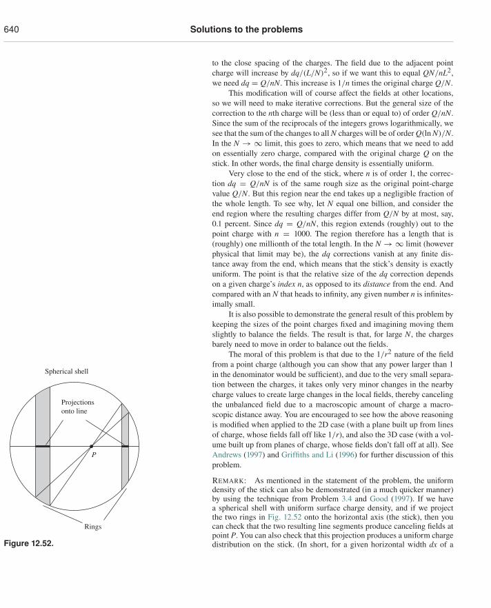
640 Solutions to the problems
to the close spacing of the charges. The field due to the adjacent pointcharge will increase by dq/(L/N)2, so if we want this to equal QN/nL2,we need dq = Q/nN. This increase is 1/n times the original charge Q/N.
This modification will of course affect the fields at other locations,so we will need to make iterative corrections. But the general size of thecorrection to the nth charge will be (less than or equal to) of order Q/nN.Since the sum of the reciprocals of the integers grows logarithmically, wesee that the sum of the changes to all N charges will be of order Q(ln N)/N.In the N → ∞ limit, this goes to zero, which means that we need to addon essentially zero charge, compared with the original charge Q on thestick. In other words, the final charge density is essentially uniform.
Very close to the end of the stick, where n is of order 1, the correc-tion dq = Q/nN is of the same rough size as the original point-chargevalue Q/N. But this region near the end takes up a negligible fraction ofthe whole length. To see why, let N equal one billion, and consider theend region where the resulting charges differ from Q/N by at most, say,0.1 percent. Since dq = Q/nN, this region extends (roughly) out to thepoint charge with n = 1000. The region therefore has a length that is(roughly) one millionth of the total length. In the N → ∞ limit (howeverphysical that limit may be), the dq corrections vanish at any finite dis-tance away from the end, which means that the stick’s density is exactlyuniform. The point is that the relative size of the dq correction dependson a given charge’s index n, as opposed to its distance from the end. Andcompared with an N that heads to infinity, any given number n is infinites-imally small.
It is also possible to demonstrate the general result of this problem bykeeping the sizes of the point charges fixed and imagining moving themslightly to balance the fields. The result is that, for large N, the chargesbarely need to move in order to balance out the fields.
The moral of this problem is that due to the 1/r2 nature of the fieldfrom a point charge (although you can show that any power larger than 1in the denominator would be sufficient), and due to the very small separa-tion between the charges, it takes only very minor changes in the nearbycharge values to create large changes in the local fields, thereby cancelingthe unbalanced field due to a macroscopic amount of charge a macro-
Spherical shell
Projectionsonto line
Rings
P
Figure 12.52.
scopic distance away. You are encouraged to see how the above reasoningis modified when applied to the 2D case (with a plane built up from linesof charge, whose fields fall off like 1/r), and also the 3D case (with a vol-ume built up from planes of charge, whose fields don’t fall off at all). SeeAndrews (1997) and Griffiths and Li (1996) for further discussion of thisproblem.
REMARK: As mentioned in the statement of the problem, the uniformdensity of the stick can also be demonstrated (in a much quicker manner)by using the technique from Problem 3.4 and Good (1997). If we havea spherical shell with uniform surface charge density, and if we projectthe two rings in Fig. 12.52 onto the horizontal axis (the stick), then youcan check that the two resulting line segments produce canceling fields atpoint P. You can also check that this projection produces a uniform chargedistribution on the stick. (In short, for a given horizontal width dx of a
12.3 Chapter 3 641
ring, a ring with a smaller radius has a smaller circumference but a largertilt angle of the surface, and these effects exactly cancel when finding thearea of the ring.) Since we can consider the stick to be completely builtup from these pairs of line segments (with a smaller piece to the rightof P, and a larger piece to the left), the field at P is therefore zero. It isamusing how this method of dividing the stick into canceling pairs of littlesegments is much more useful than the seemingly more natural methodinvolving segments equidistant from P, which is the one we used abovein Fig. 12.51.
There is actually no need to make use of the above projection of asphere (which in turn makes use of the 1/r2 nature of the electric force) todemonstrate that a uniform stick yields zero net field at any given point P.Given a uniform stick, and given a 1/rd force law with d > 1, we candivide the stick into pairs of corresponding little segments whose fieldcontributions cancel at P. We can start with corresponding little segmentsat the ends of the stick and then work our way inward to P. For a given pairof canceling segments, the segment that is farther from P will be longer(assuming d > 0, so that the field falls off with distance). More impor-tantly, if d > 1 it will be enough longer so that (as you can show) the pairswill eventually be essentially the same distance from P when they getvery close to P; P is therefore located at the center of the effective stickthat is left over after ignoring all the canceled corresponding pairs. Thenet field at P is therefore zero. In contrast, if d = 1, then, as we work ourway inward toward P, you can show that the corresponding little segmentsmaintain the same ratio of their distances from P. Since these distancesremain unequal (assuming P isn’t located exactly at the center of the orig-inal stick), P remains off-center in the effective stick that is left over afterignoring the canceled pairs. The field at P is therefore nonzero. Hence thecharge distribution on a conducting stick, in a world with a 1/r electricforce, is not uniform. Can you determine what it is?
3.6 A charge inside a shellThe reasoning is incorrect. The charge will feel a force. The error is thatthe reasoning takes a solution for one boundary condition and appliesit to a situation with another boundary condition. A consequence of theuniqueness theorem is that if we have a surface with constant potentialand no charges inside, then the constant-φ solution must be the solution.This (true) statement has nothing to do with the given setup containing apoint charge. So for the given setup, we can draw no conclusions from theabove statement, no matter how true it is. (Physically, there is a nonzeroforce because the dominant effect is that the charges induced on the nearerpart of the shell will attract the given point charge.)
3.7 Inside/outside asymmetryElectrostatic field lines can begin and end only at charges or at infinity.Also, there can be no closed loops since curl E = 0. See Problem 2.29.
If the point charge is located outside the shell, the field lines can havetheir ends at the point charge, the shell, or infinity. There can’t be any fieldlines inside the shell because they would have to start at one point on theshell and end at another. This would imply a nonzero potential differencebetween these two points, contradicting the fact that all points on the shellhave the same potential.
642 Solutions to the problems
If the point charge is located inside the shell, the field lines startingat the point charge must end up on the shell. And there can be field linesoutside the shell because they can have one end on the shell and the otherend at infinity.
We see that the basic difference between inside and outside is that theinside region has only one boundary (the shell), while the outside regionhas two (the shell and infinity). The former case therefore requires theexistence of an additional termination point (a charge) if field lines areto exist.
3.8 Inside or outsideAs we increase the size of shell A, the field at P remains zero. When we hitthe infinite-plane transition between the two cases, the field is still zero. Aswe then transition to a very large shell B surrounding the charge q, the fieldat P is very small. One way of seeing this is that there is a large amount ofinduced negative charge on the shell close to the charge q (almost as muchas on the infinite plane), and this charge nearly completely shields the fieldof the charge q at point P. Alternatively, from the example in Section 3.2,a point charge inside a conducting spherical shell looks like an equal pointcharge at the center, as far as the external field goes. And the center of avery large shell B is very far to the left. So the field at P due to the effectivepoint charge at the distant center is very small.
As we decrease the size of B, the field at P increases because notas much induced charge can pile up (due to the mutual repulsion andincreased curvature), or equivalently because the center of B moves closer.The field at P therefore increases to a finite value. In short, the field goesfrom being zero to nonzero by transitioning in a perfectly reasonable con-tinuous manner.
Although the above reasoning is correct, you might still be wonderingabout the lack of symmetry between inside and outside. If a charge isoutside a conductor, then there is no field on the other side (the inside).But if a charge is inside a conductor, then there is a field on the other side(the outside). Why should inside and outside be different? Sure, outside isbigger, but should that really matter? Actually, yes.
Consider a neutral conductor with no other charges around, and let’ssay we want to put a charge either inside or outside. To create a positivecharge, we can take a neutral object and split it into positive and neg-ative pieces, and then get rid of the negative piece. If we do this out-side the conductor, then we (1) start with zero field inside the conductor(and outside, too), then (2) create two opposite charges outside and sepa-rate them; the field is still zero inside (but not outside now), then (3) getrid of the negative charge by bringing it out to infinity; the field is stillzero inside.
However, if we try to do this inside the conductor, then we (1) startwith zero field outside the conductor (and inside, too), then (2) create twoopposite charges inside and separate them; the field is still zero outside(but not inside now), then (3) get rid of the negative charge by. . . uh oh,it’s stuck inside the conductor, so we can’t bring it out to infinity. If we doso, then the charge has to cross the conductor and enter a different region.This breaks the symmetry with the other case, so it’s no surprise that we
12.3 Chapter 3 643
end up with a different result. More precisely, the amount of charge insidethe conductor abruptly changes. In the first case, the amount of chargeoutside the conductor doesn’t change when the negative charge is broughtout to infinity. See Nan-Xian (1981) for further discussion of this. Prob-lem 3.7 presents another way in which inside and outside fundamentallydiffer.
3.9 Grounding a shellThe field outside the outer shell is zero, so the potential at the outer shellis the same as the potential at infinity. The charge will therefore not movewhen the outer shell is grounded. If some negative charge did flow off,then there would be a net positive charge on the two shells, and hence anoutward-pointing field for r > R2. This would drag the negative chargeback onto the outer shell. Likewise, if some positive charge flowed off,then there would be an inward-pointing field for r > R2 which would dragthe positive charge back onto the shell.
If the inner shell is grounded, it must end up with the amount ofcharge that makes its potential equal to the potential at infinity. Let the finalcharge be Qf. Then the electric field between the shells equals Qf/r2 (we’llignore the 1/4πε0 in this problem since it will cancel). So the potentialof the outer shell relative to the inner shell is −Qf(1/R1 − 1/R2). Sim-ilarly, the electric field outside the outer shell equals (−Q + Qf)/r2, sothe potential of the outer shell relative to infinity is (−Q + Qf)(1/R2). Ifthe inner shell and infinity are at the same potential, then the previous twopotential differences must be equal. This gives
Qf
(1
R1− 1
R2
)= (Q − Qf)
1R2
�⇒ Qf = R1R2
Q. (12.148)
Intuitively, if none of the charge leaves (so Qf = Q), then the inner shellis at a higher potential than the outer shell, which in turn is at the samepotential as infinity in this case. On the other hand, if all of the chargeleaves (so Qf = 0), then the inner shell is at the same potential as theouter shell, which in turn is at a lower potential than infinity in this case.So, by continuity, there must be a value of Qf that makes the potential ofthe inner shell equal to the potential at infinity.
3.10 Why leave?Charge will indeed flow off the inner shell out to infinity, up to the (veryshort) time when the charge on the shell equals the value calculated inProblem 3.9. The error in the opposing logic is the following. If we con-sider one small point charge, then this charge would be happy to hang outon the wire right at the hole in the outer shell. However, if we try to do thesame thing with another small point charge, then we can’t put both of themin the same place, because they will repel each other. So we certainly can’tpile up charge right at the hole in the outer shell. What if we stretch outthe charge and create a linear density along the wire? Could the chargesstabilize in a linear distribution, partially between the shells and partiallyoutside the outer shell?
To answer this, we must use the fact that a very thin wire has essen-tially zero capacitance (see Exercise 3.59; the outer radius in that setup
644 Solutions to the problems
can be assigned some arbitrary fixed value). So charge can’t pile up on thewire. If we give the wire a tiny radius, then in a static situation only a tinybit of charge can pile up. The very strong forces (which go like 1/d2, fromCoulomb’s law) between nearby charges on the wire will make the linearcharge density λ nearly uniform (see Problem 3.5). So in a sense we havean essentially rigid stick of (a tiny bit of) charge extending from the innershell out to a very large radius. The question is: what is the direction ofthe net force on this stick? Will it be drawn inward or be pushed outward?There are competing effects, because the field E1(r) between the shellspoints outward, and the field E2(r) outside the outer shell points inward(at least once some charge has left the inner shell, leaving behind a netnegative charge on the two shells). We are ignoring the forces between thecharges in the stick here, because they are internal.
Assuming constant density λ, the outward force on the stick equals∫ R2R1
E1λ dr, and the inward force equals∫∞
R2E2λ dr (this is negative since
E2 is negative). The stick won’t move if these two forces add up to zero:
∫ R2
R1
E1λ dr +∫ ∞
R2
E2λ dr = 0
�⇒∫ R2
R1
E1 dr =∫ R2
∞E2 dr
�⇒ φ(R1) − φ(R2) = φ(∞) − φ(R2)
�⇒ φ(R1) = φ(∞). (12.149)
We see that the stick won’t move if the potential at the inner shell equalsthe potential at infinity. So charge will flow off the inner shell until thetime when this condition is met, at which point the charge equals the valuecalculated in Problem 3.9.
If the wire does have a nonzero capacitance, then things are different.If we have, say, a little spherical bulge in the wire somewhere outside, thencharge will build up there, but only until the potential equals the potentialeverywhere else along the wire.
As an exercise, you can think about an analogous setup involving twolarge capacitor sheets separated by a small distance, with charges ±Q, andwith one sheet grounded by connecting it to infinity via a very thin wirethat passes through a very small hole in the other sheet.
Note that the above reasoning took advantage of the fact that∫
E drhas two interpretations. It equals the potential difference φ, of course. Butif we multiply it by a constant λ, it also equals the total force on a uni-form stick. Basically, multiply
∫E dr by q and you get the total work
done on a charged particle moving between two given points. Multiplyit by λ and you get the total force on a charged stick lying between thetwo points.
3.11 How much work?When the charge Q is a distance x above the plane, the force required tobalance the electrostatic force and move the charge upward (at constantspeed) is Q2/4πε0(2x)2, because the force is the same as if the plane