Electrical Transmission Systems and Smart Grids || Smart Grids, Distributed Control for

Chapter 6

Smart Grids, Distributed Control for

Frank Kreikebaum and Deepak Divan

Glossary

Flexible AC transmission

system (FACTS)

A system deployed on the electrical network to

control one or more parameters of the network.

FACTS is typically realized with solid-state or

mechanical switches.

Optimal power flow (OPF) A method to control generation and transmission

assets to minimize cost of operation, operate assets

at or below rated values, and meet reliability

requirements.

Reactive power One of the two forms of power in AC power trans-

mission, reactive power is the energy stored in mag-

netic and capacitive devices that is returned to the

system every cycle. Reactive power is required to

maintain grid functionality and is measured in (volt-

ampere reactive) VARs. By definition, capacitors

generate reactive power, and inductors consume

reactive power.

F. Kreikebaum

Georgia Institute of Technology, Atlanta, GA, USA

e-mail: [email protected]

D. Divan (*)

School of Electrical and Computer Engineering, Georgia Institute of Technology,

Atlanta, GA, USA

e-mail: [email protected]

This chapter was originally published as part of the Encyclopedia of Sustainability Science

and Technology edited by Robert A. Meyers. DOI:10.1007/978-1-4419-0851-3

M.M. Begovic (ed.), Electrical Transmission Systems and Smart Grids:Selected Entries from the Encyclopedia of Sustainability Science and Technology,DOI 10.1007/978-1-4614-5830-2_6, # Springer Science+Business Media New York 2013

159

mailto:[email protected]

mailto:[email protected]

http://dx.doi.org/10.1007/978-1-4419-0851-3

Definition of Distributed Control for Smart Grids

Distributed control for smart grids is the use of distributed grid assets to achieve

desired outcomes such as increased utilization of transmission assets, reduced cost of

energy, and increased reliability.Distributed control is a key enabler tomeet emerging

challenges such as load growth and renewable generation mandates.

Introduction

The utility grid is a massive system with tens of thousands of generators, hundreds

of thousands of miles of high-voltage transmission lines and millions of assets such

as transformers and capacitors, all working with split-second precision to deliver

reliable electrical energy to hundreds of millions of customers. The grid was

designed at a time when electromechanical controls and generator excitation

control were the only available control handles to keep the system operating. In

addition, the inability to guide electricity flows and to store electricity inexpen-

sively forced the adoption of rules that distorted market operation, and created

inefficient use of assets. The decision of the US government to make electricity

a universal right of the people and a regulated industry, further removed drivers that

moved the industry toward effective and competitive operation. The result of these

technology limitations and policy structures that were created, with the best of

intentions, is that the electricity markets work ineffectively at best.

The electricity industry asset base in the USA is worth an estimated $2.2 trillion

in terms of replacement value. Global and US electrical demands are expected to

rise 80% and 24%, respectively over the next 20–25 years. In the USA, if grid-

enabled vehicles (GEVs) are widely adopted, total electrical demand could be 45%

higher in 2035 than 2008. Mandates for renewable energy are expected to require

a doubling in annual transmission investment yet will lower utilization of the

transmission system. A ubiquitous roll-out of smart grid functionality would pro-

vide better utilization of the transmission and distribution system, reduce the

investment required to meet renewable mandates, and raise reliability. However,

there is no economic basis for implementing such a far-reaching transformation. It

is however possible, with correctly defined priorities, to implement an upgrade of

selected portions of the grid, to achieve a large part of the important gains. Selective

introduction of newer technologies that allow dynamic granular control (DGC) of

voltage and power flows on the grid can enable a much more efficient use of grid

assets, minimizing the need to build new transmission lines to accommodate

variable generation resources such as wind and solar.

Such control capability will transform the electricity market, allowing

transactions between willing generators and users, along pathways that have the

capacity to handle more power. It will directly mitigate problems of cost allocation

that have plagued transmission-line building. It will reduce the cost of absorbing

160 F. Kreikebaum and D. Divan

more wind and solar energy, and of adopting GEVs to improve energy security and

to reduce carbon emissions. This control cannot be implemented at the traditional

generation excitation controls, but has to be implemented at various points on the

grid, so that the utilization of diverse grid assets can be improved substantially.

Such control will necessarily be distributed in nature, and points to a future vision

of grid control.

Distributed control is a key enabler to meet emerging challenges in the electric

power sector. This entry begins by surveying the emerging challenges. It then

discusses general methods for two types of distributed control, namely VAR control

and power flow control. Next, the technologies currently available to realize VAR

control and power flow control are discussed. It then surveys emerging technologies

and methods before concluding.

Emerging Challenges

Load Growth

Globally, electrical energy demand is expected to grow 2.5% per year from 2006 to

2030 with total demand rising from 15,665 TWh in 2006 to 28,141 TWh in 2030

[1]. Worldwide generation capacity is expected to grow 2.3% per year from 2006 to

2030, rising from 4,344 to 7,484 GW [1]. The DOE Energy Information Agency

(EIA) expects US electrical load to increase 1% annually to 2035, a 24% increase

in annual demand relative to 2010 demand [2]. These projections include negligible

amounts of GEVs with electricity supplying less than 3% of global transport

energy and 0.2% of US light-duty transit sector energy in 2030 and 2035, respec-

tively [1, 3]. Historically, load growth has required investment in generation as well

as the transmission and distribution systems. Utilities are facing pressure to meet

this load growth at low cost to consumers, a challenge given high costs for fuel and

materials.

Challenges Permitting Urban Generation and Transmission

The need for distributed control can be mitigated through the installation of

generation in load centers or new transmission connecting distant generation with

load centers. Siting generation in load centers is difficult due to noise, emissions,

viewshed concerns, land acquisition cost, and the limited capacity of the urban fuel

delivery system. In addition, generator cooling water availability is projected to be

limited in many load centers [4]. A study in the USA shows that 19 of the 22

counties identified as most at risk for water shortage due to electricity generation

are located in the 20 fastest growing metropolitan statistical areas.

6 Smart Grids, Distributed Control for 161

Construction of new transmission to supply load centers is also difficult.

Concerns include viewshed, land acquisition cost, and electromagnetic radiation.

High-voltage transmission lines require more than a decade to build. Also, the

allocation of cost is problematic, especially for lines that cross state and utility

boundaries. Finally, the construction of new lines increases the MW-miles of line

serving a given amount of load, decreasing rather than increasing utilization of the

existing system, leading to cost increases and inefficiencies.

Policy Drivers for Renewable Generation

Policies are driving the adoption of renewable generation around the world. China

aims to increase renewable energy from 7.1% of total electrical energy in 2005 to

20% in 2020 with the installed wind capacity rising from 1,260 MW in 2005 to

30,000 MW in 2020 [5]. Grid operators in China are required to accommodate

renewable energy, with prices for wind decided in an auction in which only wind

plants participate [5]. In the USA, 29 states plus the District of Columbia have

enacted binding renewable portfolio standards (RPSs), and 7 states have voluntary

goals [6]. RPSs require a certain percentage of annual electrical energy demand to

be met with renewable generation by a specified year. In addition, the US federal

government incents the development of renewable generation through the Produc-

tion Tax Credit (PTC) and the US Treasury Section 1603 Investment Tax Credit.

The renewable mandates stress the transmission system and require additional

investment. One metric of this stress is the ratio of peak generation capacity to

average power demanded. In 2008, the US ratio was 2.18. In the EIA 2035

reference scenario, which sources 5% of national electricity from nonhydro

renewables resources, the ratio improves to 2.03. All things being equal, this

reduction shows increased utilization of the generation fleet in 2035 relative to

2008 and lower unit cost of energy. If a 20% RPS is mandated, the ratio rises to

2.29, a degradation resulting in lower utilization in 2035 relative to 2008. So, while

the 2035 nonrenewable case shows a 7% increase in utilization, the RPS case shows

a 5% degradation. To avoid curtailment of renewables, transmission must be built

to accommodate the peak power output of the renewable fleet.

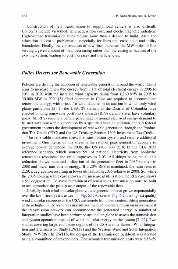
Globally, both wind and solar photovoltaic generation have grown exponentially

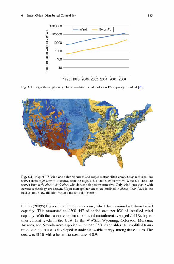
over the last fifteen years, as seen in Fig. 6.1. As seen in Fig. 6.2, the highest quality

wind and solar resources in the USA are remote from load centers. Siting generation

at these high-quality resources maximizes the plant owner’s return on investment if

the transmission network can accommodate the generated energy. A number of

integration studies have been performed around the globe to assess the transmission

and system operation impacts of wind and solar energy on the system [7–22]. Two

studies covering large, multistate regions of the USA are the Eastern Wind Integra-

tion and Transmission Study (EWITS) and the Western Wind and Solar Integration

Study (WWSIS). In EWITS, the design of the transmission build-out was iterated

using a committee of stakeholders. Undiscounted transmission costs were $33–59


billion (2009$) higher than the reference case, which had minimal additional wind

capacity. This amounted to $300–447 of added cost per kW of installed wind

capacity. With the transmission build-out, wind curtailment averaged 7–11%, higher

than current levels in the USA. In the WWSIS, Wyoming, Colorado, Montana,

Arizona, and Nevada were supplied with up to 35% renewables. A simplified trans-

mission build-out was developed to trade renewable energy among these states. The

cost was $11B with a benefit-to-cost ratio of 0.9.

1

10

100

1000

10000

100000

1000000

1996 1998 2000 2002 2004 2006 2008

Tot

al In

stal

led

Cap

acity

(G

W) Wind Solar PV

Fig. 6.1 Logarithmic plot of global cumulative wind and solar PV capacity installed [23]

Fig. 6.2 Map of US wind and solar resources and major metropolitan areas. Solar resources are

shown from light yellow to brown, with the highest resource sites in brown. Wind resources are

shown from light blue to dark blue, with darker being more attractive. Only wind sites viable with

current technology are shown. Major metropolitan areas are outlined in black. Gray lines in the

background show the high-voltage transmission system


For a scenario in which 20% of US demand is met with renewable energy, the

estimated transmission cost is $360 billion over 25 years, or $14 billion per year.

This assumes the average distance between renewable generation and load is 1,000

miles, a reasonable scenario if renewable generation is installed in high resource

areas in the Midwest and Southwest. Currently, total transmission investment,

including long-distance and local transmission, is $9 billion per year. If renewable

energy transmission investment substitutes for 50% of the current investment, total

annual investment would be $18.5 billion per year, a 105% increase over current

investment levels. This increased level of investment would need to be sustained for

25 years to supply 20% of projected US demand with renewable energy.

Policy Drivers for GEVs

Grid-enabled vehicles (GEVs) are experiencing a renaissance following their last

resurgence in the 1990s.Mainstreammanufacturers and new entrants offer or plan to

offer GEVs spanning a broad price range. In the USA, GEVs are currently supported

through federal and state tax credits. Proposals have been developed to electrify 75%

of the miles traveled by the light-duty fleet by 2040 [24]. In Europe, high fuel taxes

and a requirement that fleet average emissions drop from 160 to 95 g CO2/km are

likely to foster GEV development [24]. The Chinese government recognizes the

ability of GEVs to improve energy security and has implemented a program to build

charging infrastructure in the 13 largest cities. It also offers a tax incentive program

for vehicles and buses on the order of $8,000 and $70,000 per vehicle, respectively

[24]. The impact of GEVs on the power system is dependent on the level of GEV

adoption, the chargingmodel, and the level of coordination between the time of charging

and the power system state. If 80% of the miles traveled by the US light-duty fleet are

electrified by 2035, annual electrical demand is projected to increase 45% relative to

2008, compared to a 24% increase without GEVs. Uncoordinated charging will lead to

overloading and accelerated aging of distribution assets [64]. The monitoring system for

distribution assets is less developed than for transmission assets, making it difficult to

proactively upgrade strained distribution assets. Without coordination of vehicle charg-

ing, significant new transmission and distribution investment will likely be required.

Differences Between the Electrical Network and Other CommodityDelivery Networks

In the USA, natural gas and petroleum pipelines have become less regulated over

the last two decades. Before the 1990s, pipeline developers submitted plans for new

pipelines to FERC. FERC selected which pipelines would be built based on its

assessment of societal needs. It was assumed that FERC could not allow competi-

tion among pipelines. Following PUC CA v. CA 1990, FERC allowed more


competition in the pipeline industry. Different rates could be charged to anchor

customers, who supported pipeline construction at an early stage, and other

customers who requested pipeline access after construction.

In petroleum pipelines, product differentiation is possible by separating

shipments via a marker liquid called transmix. As of 2005, most shipment of oil

was regulated by FERC, but refined products based on petroleum used market-

based rates [25, 26]. However, market-based rates are the fastest growing rate type

[25]. FERC permits the use of market rates on a case by case basis after ensuring

that the pipeline does not have an unreasonable level of market power.

Due to deregulation, by 2000, the natural gas pipelines were no longer

guaranteed a rate of return [27]. Users who reserved capacity were given firm

transmission rights. Tariffs for firm capacity were regulated [28]. Remaining

capacity was sold in bulletin boards at market rates. Owners of capacity can resell

their capacity to realize arbitrage opportunities.

The electric network is considered a natural monopoly due to the inability of

transmission line owners to control the flow of power through their lines. This lack

of control means owners cannot take bids for the use of their lines, as is done in

natural gas pipelines. The lack of control creates free-rider effects whereby entities

benefit from investments made by others. Collectively, this creates a disincentive

for transmission owners to upgrade their assets.

Reliability Challenges in Emerging Economies

A country-wide overview of reliability statistics was not identified for the emerging

economies. Statistics for 1997–2008 were found for five utilities in Brazil, serving

a combined electrified population of 389 million [29]. Statistics were also found for

two power companies in India, the North Delhi Power Limited (NDPL) and the

Bangalore Electricity Supply Company (BESCOM) [30]. Compared to the USA,

the Brazilian utilities had eight times the annual outage duration and 14 times the

annual outage frequency. The BESCOM system had 20 times the US outage

duration. It is anticipated that continued economic growth will require more reliable

supply of electricity, necessitating investment in emerging economies.

Distributed Control Techniques

Distributed control has been used to operate the electrical system since its incep-

tion. The initial subsection of this section will describe optimal power flow (OPF),

which traces its history back to the earliest days of power system operation. Today’s

power system relies primarily on OPF to realize control. As discussed in the

previous section, numerous challenges are emerging for power system investment


and operation. Accommodating renewable energy and GEVs will likely require

a response time not possible with traditional control techniques such as OPF. This

section will introduce VAR control and power flow control. Realized with appro-

priate technologies, VAR control and power flow control can provide fast-

responding control, called dynamic granular control (DGC), to meet the emerging

challenges.

The techniques described in this section can be applied to both the transmission

and distribution systems. Controllability of the distribution system has lagged

behind that of the transmission system. This is in part due to the large number of

distribution assets, relative to transmission assets. The number of assets increases

the complexity and cost of controlling the distribution system. Unlike the transmis-

sion system, the distribution system has traditionally been operated as a radial

network rather than a meshed network. This simplifies control but leads to lower

reliability. Smart grid activities to date have been largely aimed at improving

control of the distribution system to improve efficiency, increase capacity without

new asset construction, and accommodate distributed generation.

Optimal Power Flow

Optimal power flow (OPF) is used by system operators and planners to minimize

the total cost of system operation. OPF is the primary control technique in today’s

grid. The main control handles, or control actions, are adjustments of the real and

reactive power injections of the generators. However, OPF can include other

control handles, such as the settings of a phase-shifting transformer (PST).

Although control decisions are typically made centrally, OPF is considered

distributed control because the control actuators, such as generators and PSTs, are

distributed throughout the system. OPF set points are not typically changed more

frequently than every 5 min. OPF is configured to provide sufficient safety margins

to accommodate unexpected events such as load forecast error, renewable genera-

tion forecast error, and contingencies. A contingency is when any one or more grid

assets, such as a power line or transformer, suddenly go offline.

The realization of OPF is different in vertically integrated and market

environments. In both, power flows are changed by directly changing the output

power of the generators. In the absence of other power flow control technologies,

OPF does not allow the control of flow in individual lines.

In a vertically integrated environment, a single utility is responsible for genera-

tion, transmission, and distribution in a given region. This utility owns all of the

assets in the region and knows the costs and technical limitations of its assets. The

inputs to the OPF are as follows:

• Generator parameters – For each generator, the maximum power output, mini-

mum power output, bus to which the generator is connected, and a cost curve are

provided to the OPF. Each cost curve describes the variable cost of operating the


unit at each potential operating point between minimum power and maximum

power. Variable cost includes fuel and variable O&M costs.

• Transmission line parameters – For each transmission line, the line impedance

values, nominal voltage, current rating, and terminal locations are specified.

• Transformer parameters – For each transformer, the transformer impedance

values, nominal voltages, current rating, and terminal locations are specified.

• Load data – The expected demand at each bus is forecasted for each time step

over which the OPF will be run.

• Contingency list – Normally, the OPF is run for a set of potential contingencies

rather than all possible contingencies to reduce the solution time.

• Stability limits – The OPF does not typically compute the stability of the

network endogenously. Rather, rules are provided to the OPF in the form of

a nomogram or lookup table to ensure that unstable solutions are avoided.

• Reserve margin – The amount of surplus generation capacity that must be

available to meet uncertainties in load and renewable forecasts as well as

generator outages.

In a market area, an independent system operator (ISO) or regional transmission

operator (RTO) runs the OPF to decide which generators will be used and at what

level. The transmission network is typically owned by regulated entities, which

may also own the distribution networks. Generators are independent of the owners

of the transmission and distribution networks. Rather than cost curves, the generator

owners submit bid curves to the ISO or RTO. The bid curves designate the

minimum price generation owners are willing to accept to generate energy over

the whole range of the generator output. In the simplest scheme, owners of the

distribution network designate how much power their customers will require, and

consumers are price takers. The other inputs to the OPF are the same as those used

by the vertically integrated utility. Using the generator bids and forecasted demand,

the ISO or RTO runs the OPF to compute the least cost dispatch of generators to

serve the load and meet security requirements.

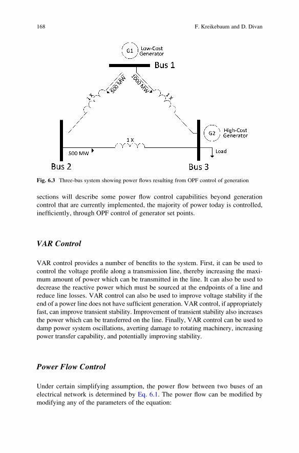
The economic impact of the lack of power flow control is visible in Fig. 6.3. In

the figure, generators, each indicated by a circle with the letter “G” inside, are

connected to bus 1 and bus 3. Load is connected at bus 3. Three transmission lines

connect the three buses. Each line has a thermal rating of 1,000 MW. All transmis-

sion lines have the same impedance X. G1 is the cheapest generator. To minimize

cost, G1 should serve the entire load at bus 3. However, due to transmission

network constraints, G1 can only supply 1,500 MW. One thousand megawatts

flows from bus 1 to bus 3 through line 1–3, and 500 MW flows from bus 1 to bus

3 via line 1–2 and line 2–3. The flow is less in line 1–2 and line 2–3 compared to

line 1–3 because of the increased impedance. Because of this impedance difference,

the flow through line 1–2 reaches the limit of 1,000 MW when the total power

transfer is 1,500 MW. This sets the maximum amount of power G1 can supply to

bus 3 even though 500 MW of unused capacity exists on line 1–2 and line 2–3.

OPF alone is limited to adjustments of generator output and is not able to resolve

numerous challenges, including those described above. While the following


sections will describe some power flow control capabilities beyond generation

control that are currently implemented, the majority of power today is controlled,

inefficiently, through OPF control of generator set points.

VAR Control

VAR control provides a number of benefits to the system. First, it can be used to

control the voltage profile along a transmission line, thereby increasing the maxi-

mum amount of power which can be transmitted in the line. It can also be used to

decrease the reactive power which must be sourced at the endpoints of a line and

reduce line losses. VAR control can also be used to improve voltage stability if the

end of a power line does not have sufficient generation. VAR control, if appropriately

fast, can improve transient stability. Improvement of transient stability also increases

the power which can be transferred on the line. Finally, VAR control can be used to

damp power system oscillations, averting damage to rotating machinery, increasing

power transfer capability, and potentially improving stability.

Power Flow Control

Under certain simplifying assumption, the power flow between two buses of an

electrical network is determined by Eq. 6.1. The power flow can be modified by

modifying any of the parameters of the equation:

Fig. 6.3 Three-bus system showing power flows resulting from OPF control of generation


• V1 and V2 are the voltage magnitudes of the endpoints of the transmission line.

• d is the angle difference between the voltage phasors at the endpoints of the

transmission line.

• X is the reactance of the transmission line.

• P is the power transmitted over the transmission line.

Voltage changes alone cannot impact power flow in a large way, since the

voltage is typically maintained within �5% of a nominal value to avoid damaging

generators, the transmission network, the distribution network, or customer

equipment.

The following sections will detail the methods used to change power flows:

Power flow between two AC buses.

P ¼ V1V2sindX

: (6.1)

Impedance Control

Impedance control of power flow aims to directly change the impedance,

represented by the value X, as seen in Eq. 6.1. Technologies able to change

impedance include the series mechanically switched capacitor (series MSC), the

series mechanically switched reactor (series MSR), the thyristor-controlled series

capacitor (TCSC), the static synchronous series compensator (SSSC), and the

unified power flow controller (UPFC). These technologies will be discussed in

more detail in section “Existing Distributed Control Technologies.”

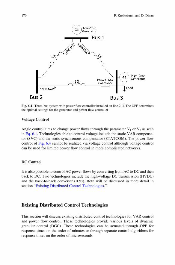
The benefit of impedance control is shown in Fig. 6.4, a modification of the

three-bus system previously shown in Fig. 6.3. Here, a power flow controller able to

change line impedance has been installed on line 2–3. Through an appropriate

modification of the impedance, the power flow in all lines can be equalized,

allowing up to 2,000 MW to be transferred between bus 1 and bus 3, compared to

the 1,500 MW using generator control alone. This allows the entire load at bus 3 to

be served by the low-cost generator, resulting in a reduction in the cost of energy.

Angle Control

Angle control aims to change power flows through the parameter d as seen in Eq. 6.1.Technologies able to control the angle include the phase-shifting transformer (PST),

also known as phase angle regulator (PAR), the variable frequency transformer™(VFT), and the solid-state transformer. The power flow control of Fig. 6.4 can also be

realized using angle control. The PST and VFT will be discussed in more detail in

section “ExistingDistributedControl Technologies.” The solid-state transformerwill

not be discussed as it is not commercially available and is expected to have high cost.


Voltage Control

Angle control aims to change power flows through the parameter V1 or V2 as seen

in Eq. 6.1. Technologies able to control voltage include the static VAR compensa-

tor (SVC) and the static synchronous compensator (STATCOM). The power flow

control of Fig. 6.4 cannot be realized via voltage control although voltage control

can be used for limited power flow control in more complicated networks.

DC Control

It is also possible to control AC power flows by converting from AC to DC and then

back to DC. Two technologies include the high-voltage DC transmission (HVDC)

and the back-to-back converter (B2B). Both will be discussed in more detail in

section “Existing Distributed Control Technologies.”

Existing Distributed Control Technologies

This section will discuss existing distributed control technologies for VAR control

and power flow control. These technologies provide various levels of dynamic

granular control (DGC). These technologies can be actuated through OPF for

response times on the order of minutes or through separate control algorithms for

response times on the order of microseconds.

Fig. 6.4 Three-bus system with power flow controller installed on line 2–3. The OPF determines

the optimal settings for the generator and power flow controller


VAR Control

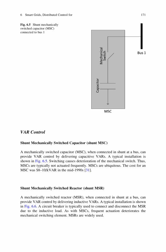
Shunt Mechanically Switched Capacitor (shunt MSC)

A mechanically switched capacitor (MSC), when connected in shunt at a bus, can

provide VAR control by delivering capacitive VARs. A typical installation is

shown in Fig. 6.5. Switching causes deterioration of the mechanical switch. Thus,

MSCs are typically not actuated frequently. MSCs are ubiquitous. The cost for an

MSC was $8–10/kVAR in the mid-1990s [31].

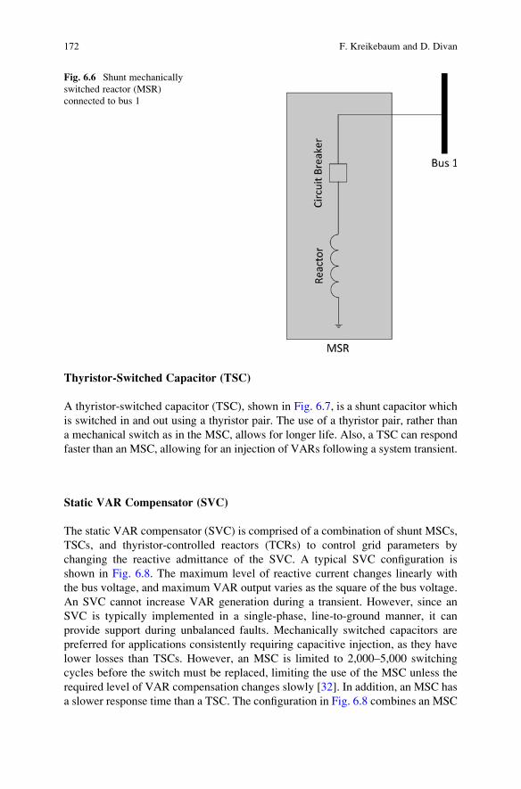
Shunt Mechanically Switched Reactor (shunt MSR)

A mechanically switched reactor (MSR), when connected in shunt at a bus, can

provide VAR control by delivering inductive VARs. A typical installation is shown

in Fig. 6.6. A circuit breaker is typically used to connect and disconnect the MSR

due to the inductive load. As with MSCs, frequent actuation deteriorates the

mechanical switching element. MSRs are widely used.

Fig. 6.5 Shunt mechanically

switched capacitor (MSC)

connected to bus 1


Thyristor-Switched Capacitor (TSC)

A thyristor-switched capacitor (TSC), shown in Fig. 6.7, is a shunt capacitor which

is switched in and out using a thyristor pair. The use of a thyristor pair, rather than

a mechanical switch as in the MSC, allows for longer life. Also, a TSC can respond

faster than an MSC, allowing for an injection of VARs following a system transient.

Static VAR Compensator (SVC)

The static VAR compensator (SVC) is comprised of a combination of shunt MSCs,

TSCs, and thyristor-controlled reactors (TCRs) to control grid parameters by

changing the reactive admittance of the SVC. A typical SVC configuration is

shown in Fig. 6.8. The maximum level of reactive current changes linearly with

the bus voltage, and maximum VAR output varies as the square of the bus voltage.

An SVC cannot increase VAR generation during a transient. However, since an

SVC is typically implemented in a single-phase, line-to-ground manner, it can

provide support during unbalanced faults. Mechanically switched capacitors are

preferred for applications consistently requiring capacitive injection, as they have

lower losses than TSCs. However, an MSC is limited to 2,000–5,000 switching

cycles before the switch must be replaced, limiting the use of the MSC unless the

required level of VAR compensation changes slowly [32]. In addition, an MSC has

a slower response time than a TSC. The configuration in Fig. 6.8 combines an MSC

Fig. 6.6 Shunt mechanically

switched reactor (MSR)

connected to bus 1


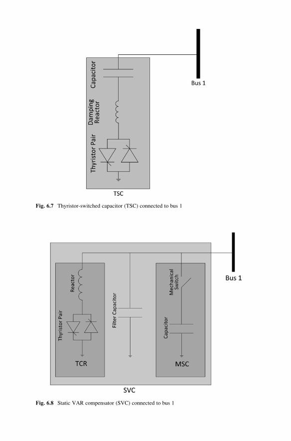
Fig. 6.7 Thyristor-switched capacitor (TSC) connected to bus 1

Fig. 6.8 Static VAR compensator (SVC) connected to bus 1

for steady-state capacitive injection with a TCR for transient performance. The

TCR generates harmonics which are removed with the shunt filters.

Worldwide, ABB has installed 499 SVCs totaling 73.3 GVAR, 54% of the

global total [33]. Of these, 228 units, with a total capacity of 49 GVAR, are for

utility customers. The remaining units are for industrial customers. Siemens has

installed at least 45 utility SVCs representing almost 10 GVAR of capacity [34].

AMSC, formerly known as American Superconductor, has installed 130 SVCs and

STATCOMs, although the breakdown between the two types is unknown [35]. An

SVC cost $50/KVAR in the mid-1990s and is expected to cost roughly $80/KVAR

now [31].

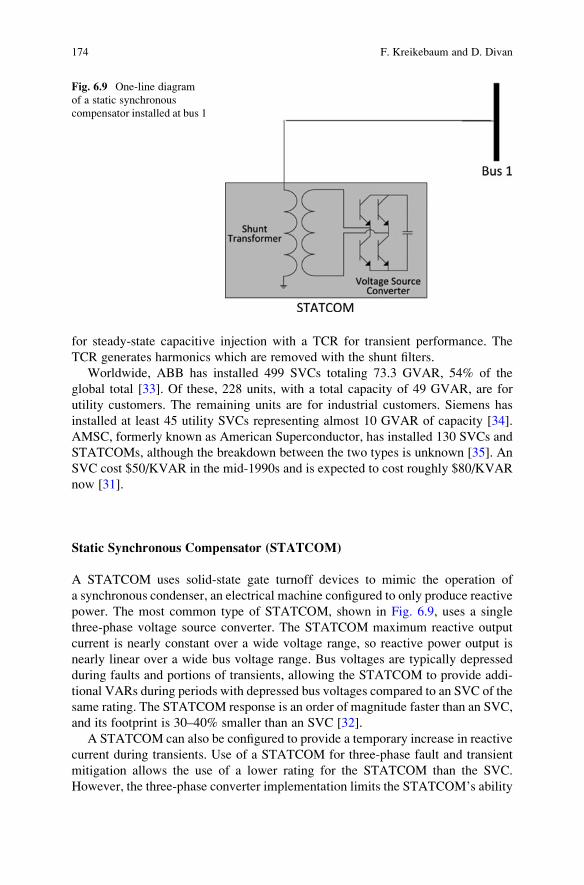
Static Synchronous Compensator (STATCOM)

A STATCOM uses solid-state gate turnoff devices to mimic the operation of

a synchronous condenser, an electrical machine configured to only produce reactive

power. The most common type of STATCOM, shown in Fig. 6.9, uses a single

three-phase voltage source converter. The STATCOM maximum reactive output

current is nearly constant over a wide voltage range, so reactive power output is

nearly linear over a wide bus voltage range. Bus voltages are typically depressed

during faults and portions of transients, allowing the STATCOM to provide addi-

tional VARs during periods with depressed bus voltages compared to an SVC of the

same rating. The STATCOM response is an order of magnitude faster than an SVC,

and its footprint is 30–40% smaller than an SVC [32].

A STATCOM can also be configured to provide a temporary increase in reactive

current during transients. Use of a STATCOM for three-phase fault and transient

mitigation allows the use of a lower rating for the STATCOM than the SVC.

However, the three-phase converter implementation limits the STATCOM’s ability

Fig. 6.9 One-line diagram

of a static synchronous

compensator installed at bus 1


to provide VARs during unbalanced faults unless the DC capacitor is significantly

overrated relative to steady-state operation. This is a significant disadvantage

compared to an SVC since an SVC can typically support unbalanced faults.

However, AREVA has implemented a STATCOM able to support unbalanced

faults through the use of separate converters for each phase.

A single, three-phase STATCOM was estimated to cost $55/kVAR in the 1990s

[31] and $150/kVAR now. A system comprised of three single-phase STATCOMs

is estimated to cost $200/kVAR.

Siemens has installed at least 14 STATCOMs [46], and ABB has installed an

unspecified number of STATCOMs. AMSC has installed 130 SVCs and

STATCOMs, although the breakdown between the two types is unknown [35].

Hybrid VAR Systems

Some installations use an SVC-STATCOM configuration, replacing the TCR of the

SVC with a STATCOM. This allows for the use of an MSC, offering lower losses

than a TSC, while retaining the quick response of the STATCOM. This also allows

for smaller filters since TCRs generate harmonics [32]. The cost and performance

characteristics lie between the SVC and STATCOM and depend on the relative

rating of the components.

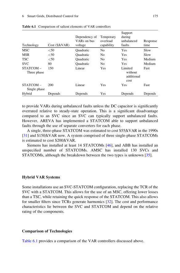
Comparison of Technologies

Table 6.1 provides a comparison of the VAR controllers discussed above.

Table 6.1 Comparison of salient elements of VAR controllers

Technology Cost ($/kVAR)

Dependency of

VARs on bus

voltage

Temporary

overload

capability

Support

during

unbalanced

faults

Response

time

MSC <50 Quadratic No Yes Slow

MSR <50 Quadratic No Yes Slow

TSC <50 Quadratic No Yes Medium

SVC 80 Quadratic No Yes Medium

STATCOM –

Three phase

150 Linear Yes Limited

without

additional

cost

Fast

STATCOM –

Single phase

200 Linear Yes Yes Fast

Hybrid Depends Depends Yes Depends Depends


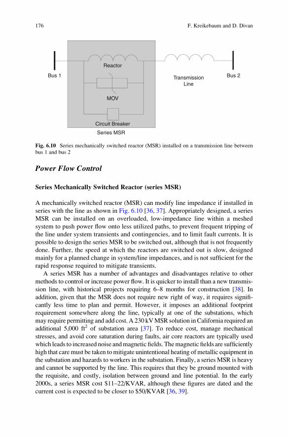
Power Flow Control

Series Mechanically Switched Reactor (series MSR)

A mechanically switched reactor (MSR) can modify line impedance if installed in

series with the line as shown in Fig. 6.10 [36, 37]. Appropriately designed, a series

MSR can be installed on an overloaded, low-impedance line within a meshed

system to push power flow onto less utilized paths, to prevent frequent tripping of

the line under system transients and contingencies, and to limit fault currents. It is

possible to design the series MSR to be switched out, although that is not frequently

done. Further, the speed at which the reactors are switched out is slow, designed

mainly for a planned change in system/line impedances, and is not sufficient for the

rapid response required to mitigate transients.

A series MSR has a number of advantages and disadvantages relative to other

methods to control or increase power flow. It is quicker to install than a new transmis-

sion line, with historical projects requiring 6–8 months for construction [38]. In

addition, given that the MSR does not require new right of way, it requires signifi-

cantly less time to plan and permit. However, it imposes an additional footprint

requirement somewhere along the line, typically at one of the substations, which

may require permitting and add cost. A 230 kVMSR solution inCalifornia required an

additional 5,000 ft2 of substation area [37]. To reduce cost, manage mechanical

stresses, and avoid core saturation during faults, air core reactors are typically used

which leads to increased noise andmagnetic fields. Themagnetic fields are sufficiently

high that caremust be taken tomitigate unintentional heating ofmetallic equipment in

the substation and hazards to workers in the substation. Finally, a series MSR is heavy

and cannot be supported by the line. This requires that they be ground mounted with

the requisite, and costly, isolation between ground and line potential. In the early

2000s, a series MSR cost $11–22/KVAR, although these figures are dated and the

current cost is expected to be closer to $50/KVAR [36, 39].

MOV

Reactor

Circuit Breaker

Series MSR

Bus 1 Bus 2TransmissionLine

Fig. 6.10 Series mechanically switched reactor (MSR) installed on a transmission line between

bus 1 and bus 2


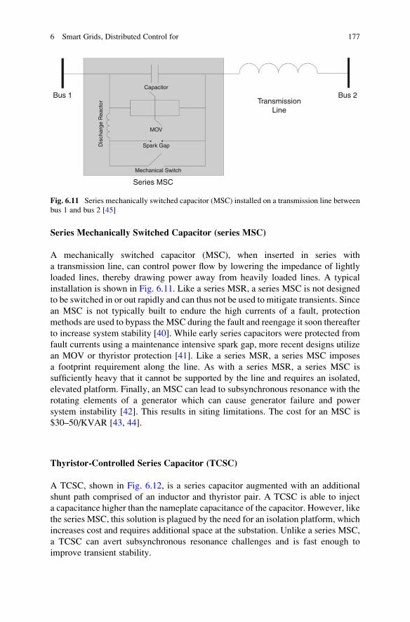
Series Mechanically Switched Capacitor (series MSC)

A mechanically switched capacitor (MSC), when inserted in series with

a transmission line, can control power flow by lowering the impedance of lightly

loaded lines, thereby drawing power away from heavily loaded lines. A typical

installation is shown in Fig. 6.11. Like a series MSR, a series MSC is not designed

to be switched in or out rapidly and can thus not be used to mitigate transients. Since

an MSC is not typically built to endure the high currents of a fault, protection

methods are used to bypass the MSC during the fault and reengage it soon thereafter

to increase system stability [40]. While early series capacitors were protected from

fault currents using a maintenance intensive spark gap, more recent designs utilize

an MOV or thyristor protection [41]. Like a series MSR, a series MSC imposes

a footprint requirement along the line. As with a series MSR, a series MSC is

sufficiently heavy that it cannot be supported by the line and requires an isolated,

elevated platform. Finally, an MSC can lead to subsynchronous resonance with the

rotating elements of a generator which can cause generator failure and power

system instability [42]. This results in siting limitations. The cost for an MSC is

$30–50/KVAR [43, 44].

Thyristor-Controlled Series Capacitor (TCSC)

A TCSC, shown in Fig. 6.12, is a series capacitor augmented with an additional

shunt path comprised of an inductor and thyristor pair. A TCSC is able to inject

a capacitance higher than the nameplate capacitance of the capacitor. However, like

the series MSC, this solution is plagued by the need for an isolation platform, which

increases cost and requires additional space at the substation. Unlike a series MSC,

a TCSC can avert subsynchronous resonance challenges and is fast enough to

improve transient stability.

Capacitor

MOV

Spark Gap

Series MSC

Bus 1 Bus 2Transmission

Line

Mechanical Switch

Dis

char

ge R

eact

or

Fig. 6.11 Series mechanically switched capacitor (MSC) installed on a transmission line between

bus 1 and bus 2 [45]


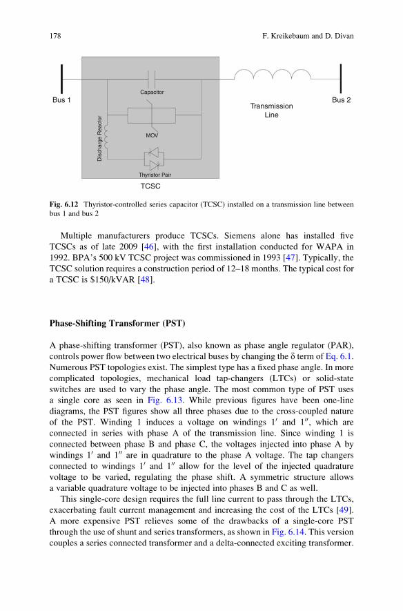
Multiple manufacturers produce TCSCs. Siemens alone has installed five

TCSCs as of late 2009 [46], with the first installation conducted for WAPA in

1992. BPA’s 500 kV TCSC project was commissioned in 1993 [47]. Typically, the

TCSC solution requires a construction period of 12–18 months. The typical cost for

a TCSC is $150/kVAR [48].

Phase-Shifting Transformer (PST)

A phase-shifting transformer (PST), also known as phase angle regulator (PAR),

controls power flow between two electrical buses by changing the d term of Eq. 6.1.

Numerous PST topologies exist. The simplest type has a fixed phase angle. In more

complicated topologies, mechanical load tap-changers (LTCs) or solid-state

switches are used to vary the phase angle. The most common type of PST uses

a single core as seen in Fig. 6.13. While previous figures have been one-line

diagrams, the PST figures show all three phases due to the cross-coupled nature

of the PST. Winding 1 induces a voltage on windings 10 and 100, which are

connected in series with phase A of the transmission line. Since winding 1 is

connected between phase B and phase C, the voltages injected into phase A by

windings 10 and 100 are in quadrature to the phase A voltage. The tap changers

connected to windings 10 and 100 allow for the level of the injected quadrature

voltage to be varied, regulating the phase shift. A symmetric structure allows

a variable quadrature voltage to be injected into phases B and C as well.

This single-core design requires the full line current to pass through the LTCs,

exacerbating fault current management and increasing the cost of the LTCs [49].

A more expensive PST relieves some of the drawbacks of a single-core PST

through the use of shunt and series transformers, as shown in Fig. 6.14. This version

couples a series connected transformer and a delta-connected exciting transformer.

Capacitor

MOV

Thyristor Pair

Dis

char

ge R

eact

or

TCSC

Bus 1 Bus 2Transmission

Line

Fig. 6.12 Thyristor-controlled series capacitor (TCSC) installed on a transmission line between

bus 1 and bus 2


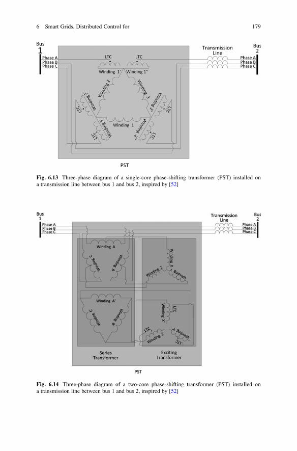
Fig. 6.13 Three-phase diagram of a single-core phase-shifting transformer (PST) installed on

a transmission line between bus 1 and bus 2, inspired by [52]

Fig. 6.14 Three-phase diagram of a two-core phase-shifting transformer (PST) installed on

a transmission line between bus 1 and bus 2, inspired by [52]


The voltages of windings Y0 and Z0 drive winding A0. The resulting winding A0

voltage is in quadrature to the phase A voltage. Winding A0 impresses a voltage

upon phase A of the line, changing the angle. Like the single-core PST, LTCs

are used to vary the level of quadrature injection. Another type of PST replaces the

mechanical LTCs with pairs of thyristors. Finally, a fifth type of PST uses voltage

source converters to synthesize the quadrature injection voltages. Although the PST

is frequently used to alter power flows, only the versions using thyristors or voltage

source converters are sufficiently fast to mitigate transients. Minimum cost for the

single-core PST is estimated to be $150/kVA. Only a fraction of a PST’s rating will

be controllable, so the actual cost per controlled kVA will be much higher.

PSTs have been identified with ratings up to 500 MW and 230 kV [50]. PSTs

have been used in WECC for at least 35 years [51]. Most PSTs deployed in the USA

can respond to operator commands or take automatic action to maintain preset

power flows in a matter of minutes [50]. The Montana Alberta Tie Limited

(MATL), believed to be the first AC merchant project in the USA, is slated to

have a PST. In the USA, there are at least 20 PSTs in WECC, at least 36 PSTs in the

Eastern Interconnection, and at least 3 in ERCOT.

High-Voltage DC Transmission (HVDC) and Back-to-Back Converter (B2B)

The high-voltage DC transmission system (HVDC) and the back-to-back converter

(B2B) transform power from AC to DC and then back to AC. Both can be used to

interconnect synchronous or asynchronous networks.

HVDC transports the power in DC form over a distance of up to thousands of

miles between the two terminals of the line. HVDC provides full control of the line

power. If HVDC is used to connect distant generation to a load pocket, the

generation is assigned the same capacity benefits as if it was located in the load

pocket [53]. Controllability and capacity benefits have incented the use of HVDC

for merchant transmission projects in the USA. In addition, the HVDC line can be

configured to limit maximum system fault current levels, an advantage over new

AC lines which tend to increase fault current. The most popular type of HVDC

system is the bipole, as shown in Fig. 6.15. In the figure, bus 1 and bus 2 are AC, and

conversion from DC to AC occurs in the HVDC terminals. Each HVDC terminal

includes a converter, a power factor correction system, and a harmonic filter. Power

factor correction is required due to the reactive power requirements of the con-

verter. Harmonic filtration is required due to the harmonics generated by the

converter. A bipole uses two conductors and does not use the earth return under

balanced operation. If one of the poles or conductors is offline, the system can

continue to operate at a fraction of rated power. When a pole or conductor is offline,

current is returned through the earth. A two-terminal, 3,000 MW bipole HVDC

system costs $70/kW for each terminal and $1 M/km [54].

A B2B is an HVDC system with the two terminals directly connected, as shown in

Fig. 6.16. The B2B consists of the same components of an HVDC, less the DC

transmission line. Like a PST, the B2B allows for the control of the power flow. Unlike


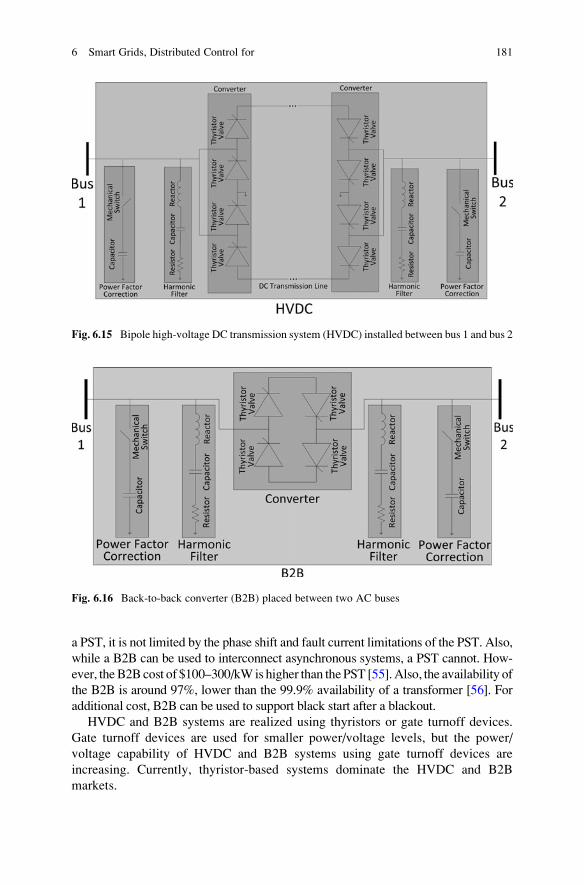
a PST, it is not limited by the phase shift and fault current limitations of the PST. Also,

while a B2B can be used to interconnect asynchronous systems, a PST cannot. How-

ever, theB2B cost of $100–300/kW is higher than thePST [55].Also, the availability of

the B2B is around 97%, lower than the 99.9% availability of a transformer [56]. For

additional cost, B2B can be used to support black start after a blackout.

HVDC and B2B systems are realized using thyristors or gate turnoff devices.

Gate turnoff devices are used for smaller power/voltage levels, but the power/

voltage capability of HVDC and B2B systems using gate turnoff devices are

increasing. Currently, thyristor-based systems dominate the HVDC and B2B

markets.

Fig. 6.15 Bipole high-voltage DC transmission system (HVDC) installed between bus 1 and bus 2

Fig. 6.16 Back-to-back converter (B2B) placed between two AC buses


In total, nearly 140 GW of HVDC and B2B capacity is installed or planned

worldwide. There are numerous B2B systems installed globally. B2Bs are installed at

the seams of the three US interconnections as well as interfaces between the US eastern

interconnection and the Hydro-Quebec system. ABB alone has completed 30 HVDC

projects and 13 B2B projects using thyristors [57] as well as 13 HVDC projects and 1

B2B project using gate turnoff devices. Siemens has installed 13 HVDC projects and

8 B2B projects using thyristor technology [58] as well as one HVDC system with gate

turnoff devices [59].

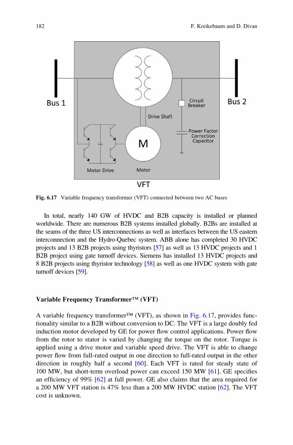
Variable Frequency Transformer™ (VFT)

A variable frequency transformer™ (VFT), as shown in Fig. 6.17, provides func-

tionality similar to a B2B without conversion to DC. The VFT is a large doubly fed

induction motor developed by GE for power flow control applications. Power flow

from the rotor to stator is varied by changing the torque on the rotor. Torque is

applied using a drive motor and variable speed drive. The VFT is able to change

power flow from full-rated output in one direction to full-rated output in the other

direction in roughly half a second [60]. Each VFT is rated for steady state of

100 MW, but short-term overload power can exceed 150 MW [61]. GE specifies

an efficiency of 99% [62] at full power. GE also claims that the area required for

a 200 MW VFT station is 47% less than a 200 MW HVDC station [62]. The VFT

cost is unknown.

Fig. 6.17 Variable frequency transformer (VFT) connected between two AC buses


GE has installed 5 VFTs at three locations. The first VFT was used to intercon-

nect the Hydro-Quebec and New York networks. The next three were installed in

parallel in Laredo, Texas. The most recent is the Linden VFT, between New York

City and New Jersey.

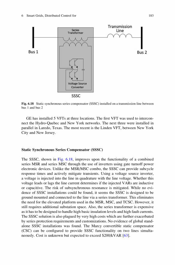
Static Synchronous Series Compensator (SSSC)

The SSSC, shown in Fig. 6.18, improves upon the functionality of a combined

series MSR and series MSC through the use of inverters using gate turnoff power

electronic devices. Unlike the MSR/MSC combo, the SSSC can provide subcycle

response times and actively mitigate transients. Using a voltage source inverter,

a voltage is injected into the line in quadrature with the line voltage. Whether this

voltage leads or lags the line current determines if the injected VARs are inductive

or capacitive. The risk of subsynchronous resonance is mitigated. While no evi-

dence of SSSC installations could be found, it seems the SSSC is designed to be

ground mounted and connected to the line via a series transformer. This eliminates

the need for the elevated platform used in the MSR, MSC, and TCSC. However, it

still requires additional substation space. Also, the series transformer is expensive

as it has to be designed to handle high basic insulation levels and high fault currents.

The SSSC solution is also plagued by very high costs which are further exacerbated

by series protection requirements and customizations. No evidence of global stand-

alone SSSC installations was found. The Marcy convertible static compensator

(CSC) can be configured to provide SSSC functionality on two lines simulta-

neously. Cost is unknown but expected to exceed $200/kVAR [63].

Fig. 6.18 Static synchronous series compensator (SSSC) installed on a transmission line between

bus 1 and bus 2


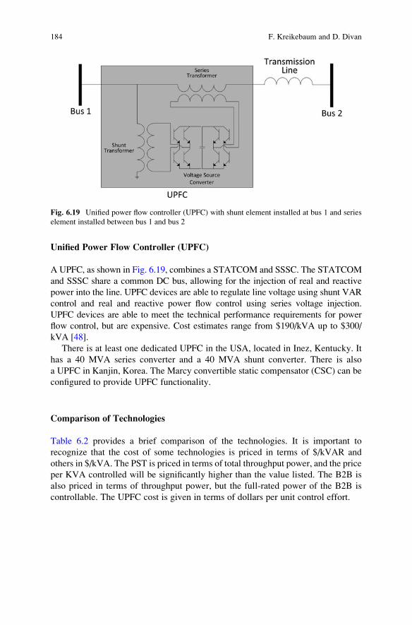
Unified Power Flow Controller (UPFC)

A UPFC, as shown in Fig. 6.19, combines a STATCOM and SSSC. The STATCOM

and SSSC share a common DC bus, allowing for the injection of real and reactive

power into the line. UPFC devices are able to regulate line voltage using shunt VAR

control and real and reactive power flow control using series voltage injection.

UPFC devices are able to meet the technical performance requirements for power

flow control, but are expensive. Cost estimates range from $190/kVA up to $300/

kVA [48].

There is at least one dedicated UPFC in the USA, located in Inez, Kentucky. It

has a 40 MVA series converter and a 40 MVA shunt converter. There is also

a UPFC in Kanjin, Korea. The Marcy convertible static compensator (CSC) can be

configured to provide UPFC functionality.

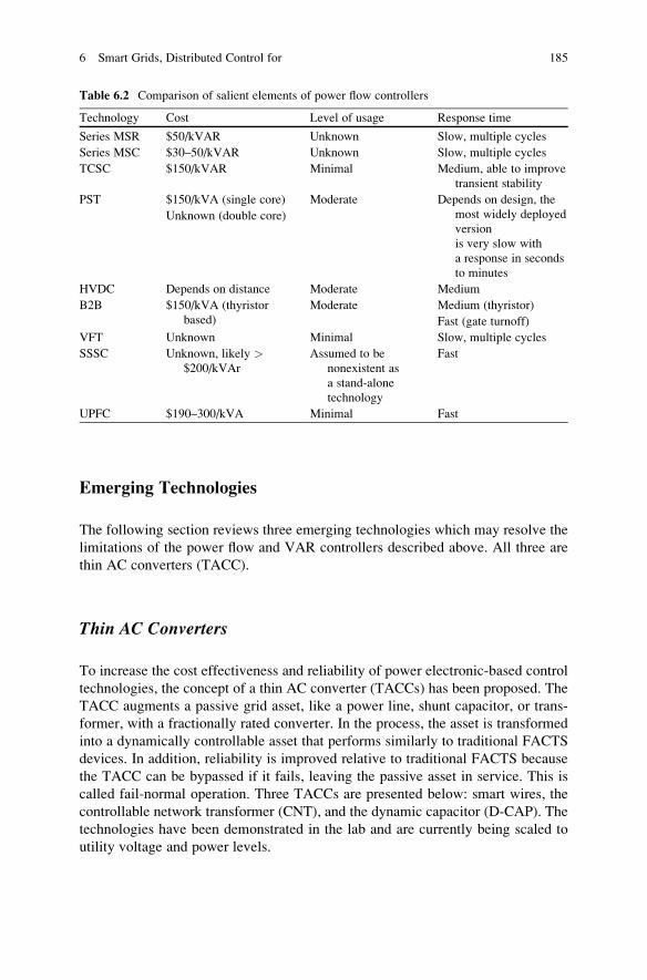
Comparison of Technologies

Table 6.2 provides a brief comparison of the technologies. It is important to

recognize that the cost of some technologies is priced in terms of $/kVAR and

others in $/kVA. The PST is priced in terms of total throughput power, and the price

per KVA controlled will be significantly higher than the value listed. The B2B is

also priced in terms of throughput power, but the full-rated power of the B2B is

controllable. The UPFC cost is given in terms of dollars per unit control effort.

Fig. 6.19 Unified power flow controller (UPFC) with shunt element installed at bus 1 and series

element installed between bus 1 and bus 2


Emerging Technologies

The following section reviews three emerging technologies which may resolve the

limitations of the power flow and VAR controllers described above. All three are

thin AC converters (TACC).

Thin AC Converters

To increase the cost effectiveness and reliability of power electronic-based control

technologies, the concept of a thin AC converter (TACCs) has been proposed. The

TACC augments a passive grid asset, like a power line, shunt capacitor, or trans-

former, with a fractionally rated converter. In the process, the asset is transformed

into a dynamically controllable asset that performs similarly to traditional FACTS

devices. In addition, reliability is improved relative to traditional FACTS because

the TACC can be bypassed if it fails, leaving the passive asset in service. This is

called fail-normal operation. Three TACCs are presented below: smart wires, the

controllable network transformer (CNT), and the dynamic capacitor (D-CAP). The

technologies have been demonstrated in the lab and are currently being scaled to

utility voltage and power levels.

Table 6.2 Comparison of salient elements of power flow controllers

Technology Cost Level of usage Response time

Series MSR $50/kVAR Unknown Slow, multiple cycles

Series MSC $30–50/kVAR Unknown Slow, multiple cycles

TCSC $150/kVAR Minimal Medium, able to improve

transient stability

PST $150/kVA (single core) Moderate Depends on design, the

most widely deployed

version

is very slow with

a response in seconds

to minutes

Unknown (double core)

HVDC Depends on distance Moderate Medium

B2B $150/kVA (thyristor

based)

Moderate Medium (thyristor)

Fast (gate turnoff)

VFT Unknown Minimal Slow, multiple cycles

SSSC Unknown, likely >$200/kVAr

Assumed to be

nonexistent as

a stand-alone

technology

Fast

UPFC $190–300/kVA Minimal Fast


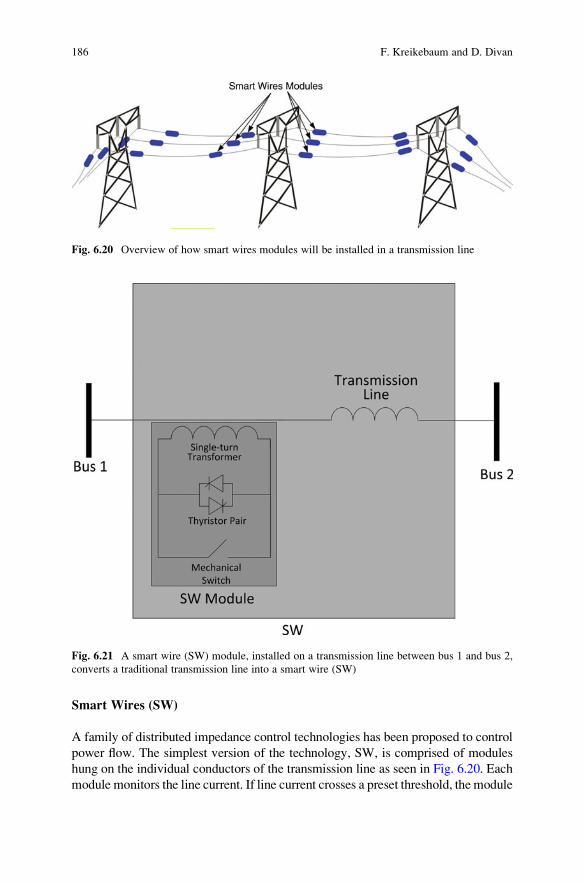
Smart Wires (SW)

A family of distributed impedance control technologies has been proposed to control

power flow. The simplest version of the technology, SW, is comprised of modules

hung on the individual conductors of the transmission line as seen in Fig. 6.20. Each

module monitors the line current. If line current crosses a preset threshold, the module

Fig. 6.20 Overview of how smart wires modules will be installed in a transmission line

Fig. 6.21 A smart wire (SW) module, installed on a transmission line between bus 1 and bus 2,

converts a traditional transmission line into a smart wire (SW)


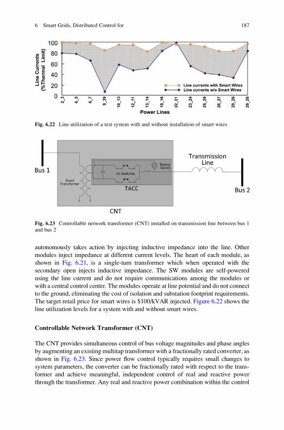
autonomously takes action by injecting inductive impedance into the line. Other

modules inject impedance at different current levels. The heart of each module, as

shown in Fig. 6.21, is a single-turn transformer which when operated with the

secondary open injects inductive impedance. The SW modules are self-powered

using the line current and do not require communications among the modules or

with a central control center. The modules operate at line potential and do not connect

to the ground, eliminating the cost of isolation and substation footprint requirements.

The target retail price for smart wires is $100/kVAR injected. Figure 6.22 shows the

line utilization levels for a system with and without smart wires.

Controllable Network Transformer (CNT)

The CNT provides simultaneous control of bus voltage magnitudes and phase angles

by augmenting an existing multitap transformer with a fractionally rated converter, as

shown in Fig. 6.23. Since power flow control typically requires small changes to

system parameters, the converter can be fractionally rated with respect to the trans-

former and achieve meaningful, independent control of real and reactive power

through the transformer. Any real and reactive power combination within the control

Fig. 6.22 Line utilization of a test system with and without installation of smart wires

Fig. 6.23 Controllable network transformer (CNT) installed on transmission line between bus 1

and bus 2


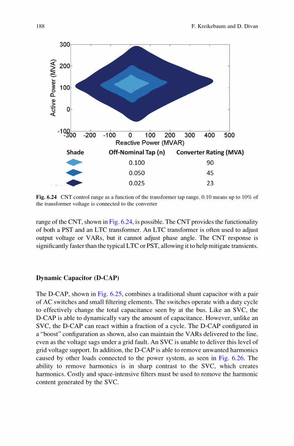
range of the CNT, shown in Fig. 6.24, is possible. The CNT provides the functionality

of both a PST and an LTC transformer. An LTC transformer is often used to adjust

output voltage or VARs, but it cannot adjust phase angle. The CNT response is

significantly faster than the typical LTC or PST, allowing it to helpmitigate transients.

Dynamic Capacitor (D-CAP)

The D-CAP, shown in Fig. 6.25, combines a traditional shunt capacitor with a pair

of AC switches and small filtering elements. The switches operate with a duty cycle

to effectively change the total capacitance seen by at the bus. Like an SVC, the

D-CAP is able to dynamically vary the amount of capacitance. However, unlike an

SVC, the D-CAP can react within a fraction of a cycle. The D-CAP configured in

a “boost” configuration as shown, also can maintain the VARs delivered to the line,

even as the voltage sags under a grid fault. An SVC is unable to deliver this level of

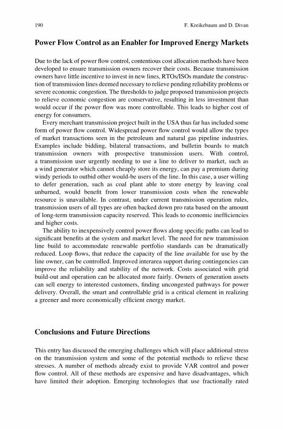
grid voltage support. In addition, the D-CAP is able to remove unwanted harmonics

caused by other loads connected to the power system, as seen in Fig. 6.26. The

ability to remove harmonics is in sharp contrast to the SVC, which creates

harmonics. Costly and space-intensive filters must be used to remove the harmonic

content generated by the SVC.

Fig. 6.24 CNT control range as a function of the transformer tap range. 0.10 means up to 10% of

the transformer voltage is connected to the converter


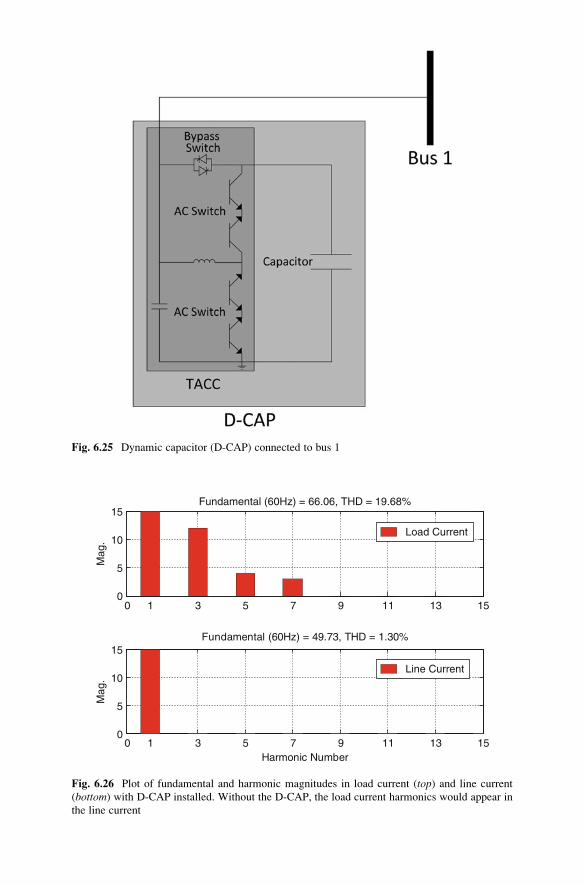
Fig. 6.25 Dynamic capacitor (D-CAP) connected to bus 1

0 1 3 5 7 9 11 13 15

0 1 3 5 7 9 11 13 15

0

5

10

15

Mag

.

0

5

10

15

Mag

.

Fundamental (60Hz) = 66.06, THD = 19.68%

Harmonic Number

Fundamental (60Hz) = 49.73, THD = 1.30%

Load Current

Line Current

Fig. 6.26 Plot of fundamental and harmonic magnitudes in load current (top) and line current

(bottom) with D-CAP installed. Without the D-CAP, the load current harmonics would appear in

the line current

Power Flow Control as an Enabler for Improved Energy Markets

Due to the lack of power flow control, contentious cost allocation methods have been

developed to ensure transmission owners recover their costs. Because transmission

owners have little incentive to invest in new lines, RTOs/ISOs mandate the construc-

tion of transmission lines deemed necessary to relieve pending reliability problems or

severe economic congestion. The thresholds to judge proposed transmission projects

to relieve economic congestion are conservative, resulting in less investment than

would occur if the power flow was more controllable. This leads to higher cost of

energy for consumers.

Every merchant transmission project built in the USA thus far has included some

form of power flow control. Widespread power flow control would allow the types

of market transactions seen in the petroleum and natural gas pipeline industries.

Examples include bidding, bilateral transactions, and bulletin boards to match

transmission owners with prospective transmission users. With control,

a transmission user urgently needing to use a line to deliver to market, such as

a wind generator which cannot cheaply store its energy, can pay a premium during

windy periods to outbid other would-be users of the line. In this case, a user willing

to defer generation, such as coal plant able to store energy by leaving coal

unburned, would benefit from lower transmission costs when the renewable

resource is unavailable. In contrast, under current transmission operation rules,

transmission users of all types are often backed down pro rata based on the amount

of long-term transmission capacity reserved. This leads to economic inefficiencies

and higher costs.

The ability to inexpensively control power flows along specific paths can lead to

significant benefits at the system and market level. The need for new transmission

line build to accommodate renewable portfolio standards can be dramatically

reduced. Loop flows, that reduce the capacity of the line available for use by the

line owner, can be controlled. Improved interarea support during contingencies can

improve the reliability and stability of the network. Costs associated with grid

build-out and operation can be allocated more fairly. Owners of generation assets

can sell energy to interested customers, finding uncongested pathways for power

delivery. Overall, the smart and controllable grid is a critical element in realizing

a greener and more economically efficient energy market.

Conclusions and Future Directions

This entry has discussed the emerging challenges which will place additional stress

on the transmission system and some of the potential methods to relieve these

stresses. A number of methods already exist to provide VAR control and power

flow control. All of these methods are expensive and have disadvantages, which

have limited their adoption. Emerging technologies that use fractionally rated


control elements, and are inherently more distributed in nature, may overcome the

significant disadvantages, allowing widespread adoption of VAR control and power

flow control. These capabilities could transform the operation of the transmission

system, enabling the delivery of low cost and renewable energy, and allowing

efficient operation of a competitive energy market.

Bibliography

1. IEA (2008)World energy outlook 2008. http://www.iea.org/textbase/nppdf/free/2008/weo2008.

pdf. Accessed 30 Mar 2011

2. EIA (2010) Table 8: electricity supply, disposition, prices, and emissions. Annual energy

outlook 2011. http://www.eia.doe.gov/forecasts/aeo/excel/aeotab_8.xls. Accessed 16 Mar

2011

3. EIA (2010) Table 46: transportation sector energy use by fuel type within mode. Annual

energy outlook 2011. http://www.eia.gov/oiaf/aeo/supplement/suptab_46.xls. Accessed 24 Apr

2011

4. Sovacool B, Sovacool K (2009) Identifying future electricity–water tradeoffs in the United

States. Energy Policy 37(7):2763–2773

5. Wang F, Yin H, Li S (2010) China’s renewable energy policy: commitments and challenges.

Energy Policy 38(4):1872–1878

6. DOE (2011) RPS data spreadsheet. http://www.dsireusa.org/rpsdata/RPSspread010211.xlsx.

Accessed 30 Mar 2011

7. NYSERDA (2004) The effects of integrating wind power on transmission system planning,

reliability, and operations: report on phase I

8. Xcel Energy, Minnesota Department of Commerce (2004) Wind integration study – Final

report

9. NYSERDA (2005) The effects of integrating wind power on transmission system planning,

reliability, and operations, report on phase 2: system performance evaluation

10. Minnesota Public Utilities Commission (2006) Final report – 2006 Minnesota Wind Integra-

tion Study, vol I

11. CEC (2007) Intermittency analysis project: final report, CEC-500-2007-081

12. Arizona Public Service Company (2007) Final report: Arizona Public Service wind integration

cost impact study

13. CA ISO (2007) Integration of renewable resources. http://www.caiso.com/1ca5/

1ca5a7a026270.pdf. Accessed 27 Oct 2010

14. ERCOT (2008) Analysis of wind generation impact on ERCOT Ancillary Services

requirements – final report

15. Xcel Energy (2008) Final report: wind integration study for Public Service of Colorado

16. SPP (2010) SPP WITF wind integration study

17. NREL (2010) Eastern wind integration and transmission study. Subcontract report NREL/SR-

550-47078

18. NREL (2010) Nebraska statewide wind integration study, Apr 2008–Jan 2010. NREL/SR-550-

47519

19. NREL (2010) Western wind and solar integration study. Subcontract No. AAM-8-77557-01

20. NYISO (2010) Growing wind: final report of the NYISO 2010 wind generation study

21. NREL (2010) Oahu wind integration and transmission study: summary report. TP-5500-48632

22. GE Energy (2010) Final report: new england wind integration study – executive summary.

Prepared for ISO New England


http://www.iea.org/textbase/nppdf/free/2008/weo2008.pdf

http://www.iea.org/textbase/nppdf/free/2008/weo2008.pdf

http://www.eia.doe.gov/forecasts/aeo/excel/aeotab_8.xls

http://www.eia.gov/oiaf/aeo/supplement/suptab_46.xls

http://www.dsireusa.org/rpsdata/RPSspread010211.xlsx

http://www.caiso.com/1ca5/1ca5a7a026270.pdf

http://www.caiso.com/1ca5/1ca5a7a026270.pdf

23. BP (2010) BP statistical review of world energy. http://www.bp.com/liveassets/bp_internet/

globalbp/globalbp_uk_english/reports_and_publications/statistical_energy_review_2008/

STAGING/local_assets/2010_downloads/Statistical_Review_of_World_Energy_2010.xls.

Accessed 24 Apr 2011

24. Electrification Coalition (2009) Electrification roadmap, Revolutionizing Transportation and

Achieving Energy Security. http://www.electrificationcoalition.org/reports/EC-Roadmap-

screen.pdf. Accessed 7 Mar 2011

25. Allegro Energy (2001) How pipelines make the oil market work their networks, operation and

regulation – a memorandum prepared for the association of oil pipe lines and the American

Petroleum Institute’s Pipeline Committee. http://www.pipeline101.com/reports/Notes.pdf.

Accessed 25 May 2009

26. Hull B (2005) Oil pipeline markets and operations. J Transp Res Forum 44(2):111–125

27. Brown S, Yucel M (2008) Deliverability and regional pricing in U.S. Natural Gas Markets.

Energy Econ 30(5):2441–2453

28. Cremer H, Gasmi F, Laffont J (2003) Access to pipelines in competitive gas markets. J Regul

Econ 24(1):5–33

29. Silvestre B, Hall J, Matos S, Figueira L (2010) Privatization of electricity distribution in the

Northeast of Brazil: the good, the bad, the ugly or the naıve? Energy Policy 38(11):7001–7013

30. Balijepalli V, Khaparde S, Gupta R (2009) Towards Indian smart grids. In: IEEE region 10

TENCON, pp 1–7

31. ORNL (1997) Ancillary service details: voltage control. ORNL/CON-453

32. Hingorani N, Gyugyi L (1999) Understanding FACTS: concepts and technology of flexible

AC transmission systems. IEEE Press, New York

33. ABB (2010) ABB SVC and SVC light projects worldwide. http://search-ext.abb.com/library/

Download.aspx?DocumentID=SVC_U%20Ref&LanguageCode=

en&DocumentPartID=&Action=Launch. Accessed 1 Apr 2011

34. Siemens (2010) FACTS – flexible AC transmission systems: static VAR compensators. http://

www.energy.siemens.com/hq/pool/hq/power-transmission/FACTS/FACTS_References_SVC.

pdf. Accessed 1 Apr 2011

35. American Superconductor (2010) AMSC™ SVC static VAR compensator. http://www.amsc.

com/pdf/PESSVC_BRO_0810_lores.pdf. Accessed 2 Apr 2011

36. Wolf G, Skliutas J et al. (2003) Alternative method of power flow control: using air core series

reactors. In: Proceedings of the IEEE Power Engineering Society General Meeting, Vol. 2

37. Bonheimer D, Lim E, Dudley R, Castanheira A (1991) A modern alternative for power flow

control. In: Proceedings of the IEEE Power Engineering Society transmission and distribution

conference, Dallas, 22–27 Sep 1991, pp 586–591

38. Papp K, Christiner G, Popelka H, Schwan M (2004) High voltage series reactors for load flow

control. e&i Elektrotechnik und Informationstechnik 121:455–460

39. Surapongpun L, Phuyodying P, Pimjaipong W (2002) New alternative of power control for

transmission line investment in Thailand. In: Proceedings of the IEEE PES transmission

and distribution conference and exhibition, Yokohama, pp 1596–1600

40. Courts A, Hingorani N, Stemler G (1978) A new series capacitor protection scheme using

nonlinear resistors. IEEE Trans Power Appar Syst 97:1042–1052

41. Bhargava B, Haas R (2002) Thyristor protected series capacitors project at Southern California

Edison Co. IEEE Power Eng Soc Summer Meet 1:241–246

42. Elfayoumy M, Moran C (2003) A comprehensive approach for subsynchronous resonance

screening analysis using frequency scanning technique. In: IEEE power tech conference

proceedings, Bologna

43. Agrawal B (2009) Reactors, capacitors, SVC, PSS: long term transmission planning seminar.

Arizona Public Service Co, Long term transmission planning seminar

44. Acharya N (2004) Facts and figures about FACTS. Presented at: AIT training workshop on

FACTS application, Asian Institute of Technology, December 16, 2004


http://www.bp.com/liveassets/bp_internet/globalbp/globalbp_uk_english/reports_and_publications/statistical_energy_review_2008/STAGING/local_assets/2010_downloads/Statistical_Review_of_World_Energy_2010.xls



http://www.electrificationcoalition.org/reports/EC-Roadmap-screen.pdf

http://www.electrificationcoalition.org/reports/EC-Roadmap-screen.pdf

http://www.pipeline101.com/reports/Notes.pdf

http://search-ext.abb.com/library/Download.aspx?DocumentID=SVC_U%20Ref&LanguageCode=en&DocumentPartID=&Action=Launch



http://www.energy.siemens.com/hq/pool/hq/power-transmission/FACTS/FACTS_References_SVC.pdf



http://www.amsc.com/pdf/PESSVC_BRO_0810_lores.pdf

http://www.amsc.com/pdf/PESSVC_BRO_0810_lores.pdf

45. Altuve H, Mooney J, Alexander G (2009) Advances in series-compensated line protection. In:

Proceedings of the 62nd Annual Conference for Protective Relay Engineers, pp 263–275

46. Retzmann D (2009) Tutorial on VSC in transmission systems HVDC & FACTS. http://www.

ptd.siemens.de/Siemens2_VS_Application_Prospects_V1.pdf. Accessed 1 Apr 2011

47. Urbanek J, Piwko R, Larsen E, Damnsky B, Furumasu B, Mittlestadt W, Eden J (1993)

Thyristor controlled series compensation prototype installation at the slatt 500 kV substation.

IEEE Trans Power Deliv 8(3):1460–1469

48. Cai L, Erlich I, Stamtsis G (2004) Optimal choice and allocation of FACTS devices in

deregulated electricity market using genetic algorithms. In: Proceedings of the 2004 IEEE

PES Power Systems Conference and Exposition, pp 201–207

49. IEEE (2010) IEEE draft guide for the application, specification and testing of phase shifting

transformers. IEEE PC57.135, Draft revision 8, Nov 2010, pp 1–53

50. Bladow J, Montoya A (1991) Experiences with parallel EHV phase shifting transformers.

IEEE Trans Power Deliv 6(3):1096–1100

51. WECC (2009) Unscheduled Flow (USF) FAQ. http://www.wecc.biz/committees/Standing-

Committees/OC/UFAS/Shared%20Documents/USF%20FAQ.doc. Accessed 20 Mar 2011

52. IEEE (2010) IEEE draft guide for the application, specification and testing of phase shifting

transformers. IEEE PC57.135_D8, pp 1–53

53. O’Neill R (2010) Merchant transmission: a new approach to transmission expansion. In:

Proceedings of the 2010 IEEE Power and Energy Society general meeting, pp 1–5

54. Bahrman M, Johnson B (2007) The ABCs of HVDC transmission technologies. IEEE Power

Energ Mag 5(2):32–44

55. Hingorani N (1996) High-voltage DC transmission: a power electronics workhorse. IEEE

Spectr 33(4):63–72

56. ABB (2011) HVDC classic reliability and availability. http://www.abb.com/industries/ap/

db0003db004333/eb8b4075fb412

52ec12574aa00409424.aspx. Accessed 5 May 2011

57. ABB (2010) HVDC classic – reference list. http://www05.abb.com/global/scot/scot221.nsf/

veritydisplay/a0f3c70bc17b846fc

12577a8004da670/$file/pow-0013%20rev10%20lr.pdf. Accessed 1 Apr 2011

58. Siemens (2011) References. http://www.energy.siemens.com/hq/en/power-transmission/hvdc/

hvdc-classic/references.htm. Accessed 1 Apr 2011

59. Siemens (2011) HVDC plus (VSC Technology). http://www.energy.siemens.com/hq/en/

power-transmission/hvdc/hvdc-plus/#content=References. Accessed 1 Apr 2011

60. Larsen E, Piwko R, McLaren D, McNabb D, Granger M, Dusseault M, Rollin L,

Primeau J (2004) Variable frequency transformer – a new alternative for asynchronous power

transfer. http://www.gepower.com/prod_serv/products/transformers_vft/en/downloads/

overview_vftmarketing.pdf. Accessed 6 Apr 2011

61. Miller N, Clark K, Piwko R, Larsen E (2006) Variable frequency transformer: applications for

secure inter-regional power exchange. Presented at PowerGen Middle East 2006. http://www.

gepower.com/prod_serv/products/transformers_vft/en/ downloads/vftfor_pgmev9.pdf.

Accessed 4 Apr 2011

62. GE (2004) Variable frequency transformer™: fact sheet. http://www.gepower.com/prod_serv/

products/transformers_vft/en/ downloads/vft_factsheet.pdf. Accessed 1 Apr 2011

63. Song W, Bhattacharya S, Huang A (2008) Fault-tolerant transformerless power flow controller

based on ETO light converter. In: Proceedings of the 2008 IEEE Industry Applications Society

annual meeting, pp 1–5

64. Moghe R, Kreikebaum F, Hernandez J, Kandula R, Divan D (2011) Mitigating distribution

transformer lifetime degradation caused by grid-enabled vehicle (GEV) charging. In:

Proceedings of the IEEE Energy Conversion Congress & Expo, Phoenix, 17–22 Sep 2011,

pp 835–842


http://www.ptd.siemens.de/Siemens2_VS_Application_Prospects_V1.pdf

http://www.ptd.siemens.de/Siemens2_VS_Application_Prospects_V1.pdf

http://www.wecc.biz/committees/StandingCommittees/OC/UFAS/Shared%20Documents/USF%20FAQ.doc

http://www.wecc.biz/committees/StandingCommittees/OC/UFAS/Shared%20Documents/USF%20FAQ.doc

http://www.abb.com/industries/ap/db0003db004333/eb8b4075fb41252ec12574aa00409424.aspx



http://www05.abb.com/global/scot/scot221.nsf/veritydisplay/a0f3c70bc17b846fc12577a8004da670/$file/pow-0013%20rev10%20lr.pdf



http://www.energy.siemens.com/hq/en/power-transmission/hvdc/hvdc-classic/references.htm

http://www.energy.siemens.com/hq/en/power-transmission/hvdc/hvdc-classic/references.htm

http://www.energy.siemens.com/hq/en/power-transmission/hvdc/hvdc-plus/#content=References

http://www.energy.siemens.com/hq/en/power-transmission/hvdc/hvdc-plus/#content=References

http://www.gepower.com/prod_serv/products/transformers_vft/en/downloads/overview_vftmarketing.pdf

http://www.gepower.com/prod_serv/products/transformers_vft/en/downloads/overview_vftmarketing.pdf

http://www.gepower.com/prod_serv/products/transformers_vft/en/downloads/vftfor_pgmev9.pdf

http://www.gepower.com/prod_serv/products/transformers_vft/en/downloads/vftfor_pgmev9.pdf

http://www.gepower.com/prod_serv/products/transformers_vft/en/downloads/vft_factsheet.pdf

http://www.gepower.com/prod_serv/products/transformers_vft/en/downloads/vft_factsheet.pdf