Embed Size (px)
Citation preview
ELECTRIC LOAD FORECAST F13-F33
P A G E 1
Electric Load Forecast Fiscal 2013 to Fiscal 2033
Load and Market Forecasting Energy Planning and Economic Development
BC Hydro
2012 Forecast December 2012
ELECTRIC LOAD FORECAST F13-F33
P A G E 2
Tables of Contents Executive Summary .................................................................................................... 7
1 Introduction ....................................................................................................... 16
2 Regulatory Background and Current Initiatives ................................................. 18
3 Forecast Drivers, Data Sources and Assumptions ............................................ 19 3.1 Forecast Drivers ................................................................................ 19 3.2 Data Sources ..................................................................................... 19 3.3 Growth Assumptions ......................................................................... 20
4 Comparison of 2011 and 2012 Forecasts ......................................................... 21 4.1 Integrated System Gross Energy Requirements before DSM with Rate
Impact ............................................................................................... 21 4.2 Total Integrated Peak Demand before DSM with Rate Impacts ......... 22
5 Sensitivity Analysis ........................................................................................... 23
6. Residential Forecast ......................................................................................... 25 6.1. Sector Description ............................................................................. 25 6.2 Forecast Summary ............................................................................ 25 6.3 Residential Forecast Comparison ...................................................... 25 6.4. Key Issues ......................................................................................... 26 6.5 Forecast Methodology ....................................................................... 27 6.6 Risks and Uncertainties ..................................................................... 27
7 Commercial Forecast ........................................................................................ 30 7.1 Sector Description ..................................................................................... 30 7.2 Forecast Summary ..................................................................................... 30 7.3 Commercial Forecast Comparison ............................................................. 30 7.4 Key Issues ......................................................................................... 31 7.5 Forecast Methodology ....................................................................... 32 7.6 Risk and Uncertainties ....................................................................... 32
8 Industrial Forecast ............................................................................................ 35 8.1 Sector Description ..................................................................................... 35 8.2 Forecast Summary ................................................................................... 35 8.3 Industrial Forecast Comparison ................................................................. 35 8.4 Key Issues and Sector Outlook .......................................................... 36 8.4.1 Forestry ............................................................................................ 36 8.4.2 Mining .............................................................................................. 40 8.4.2 Oil and Gas ....................................................................................... 44 8.4.3. Other Industrials ................................................................................ 44
9 Non-Integrated Areas and Other Utilities Forecast ............................................ 48 9.1. Non Integrated Area Summary .......................................................... 48 9.2 Other Utilities & Firm Export .............................................................. 52
10 Peak Demand Forecast .................................................................................... 54 10.1 Peak Description ............................................................................... 54 10.2 Peak Demand Forecast .................................................................... 54 10.3 Peak Forecast Comparison .............................................................. 55 10.3.3 Integrated System Peak ......................................................................... 59 10.5 Risks and Uncertainties........................................................................... 62
Appendix 1 Forecast Processes and Methodologies ................................................ 66 A1.1. Statistically Adjusted Forecast Methodology ..................................... 66 A1.2. Industrial Forecast Methodology ........................................................ 69

ELECTRIC LOAD FORECAST F13-F33
P A G E 3
A1.3. Peak Demand Forecast Methodology ................................................ 73
Appendix 2 - Monte Carlo Methods ........................................................................... 77
Appendix 3.1 - Oil and Gas (transmission serviced) ................................................. 82
Appendix 3.2 - Shale Gas Producer Forecast – (Montney) ....................................... 86
Appendix 3.3 – LNG Load Outlook ........................................................................... 94
Appendix 4 - Electric Vehicles (EVs) ......................................................................... 95
Appendix 5 - Codes and Standards Overlap with DSM ........................................... 102
Appendix 6 - Forecast Tables ................................................................................. 107
ELECTRIC LOAD FORECAST F13-F33
P A G E 4
Tables Table E1 Comparison of Integrated System Energy before DSM with Rate Impacts ...... 11
Table E2 Comparison of Integrated System Peak Demand before DSM with Rate Impacts ..................................................................................................................... 11
Table E3. Reference Energy and Peak Forecast before DSM and With Rate Impacts ... 14
Table 3.1. Key Forecast Drivers ................................................................................ 19
Table 3.2. Data Sources for the 2012 Load Forecast ............................................... 19
Table 3.3. Growth Assumptions (Annual rate of growth) ............................................ 20
Table 4.1 Comparison of Integrated Gross System Requirements Before DSM With Rate Impacts (Including Impacts of EVs and Overlap for Codes and Standards) (GWh) ... 21
Table 4.2. Comparison of Integrated Gross System Requirements Before DSM With Rate Impacts (Including Impacts of EVs and Overlap for Codes and Standards) (MW) ................................................................................................................................. 22
Figure 7.1 Comparison of Commercial Sales Forecast before DSM with Rate Impacts . 31
Table 7.1 Commercial Sales before DSM with Rate Impacts ........................................ 34
Table 8.1 Consolidated Industrial Forecast by Sector before DSM and Rate Impacts ...... 46
Table 8.2 Industrial Forecast by Voltage Service before DSM and Rate Impacts ........... 47
Table 9.1 NIA Total Sales before DSM with Rate Impacts (GWh) ................................... 50
Table 9.2 Non Integrated Area Peak Requirements before DSM with Rate Impacts (MW) ................................................................................................................................. 51
Table 10.1 Comparison of BC Hydro’s Distribution Peak Demand Forecasts before DSM with Rate Impacts ..................................................................................................... 56
Table 10.2 Comparison of BC Hydro’s Transmission Peak Demand Forecast before DSM with Rate Impacts ............................................................................................ 58
Table 10.3 Comparison of Total Integrated Peak Demand Forecast before DSM with Rate Impacts ................................................................................. 59
10.4 Peak Demand Forecast Methodology ...................................................................... 60
Table A1.1 Industrial Distribution Forecast before DSM and Rates .................................. 70
Table A2.1. Elasticity Parameter for Monte Carlo Model .................................................. 79
Table A2.2. Triangular distribution for random variable in Monte Carlo Model ................. 80
Table A3.1 Montney Gas Production and Sales Forecasts – Before DSM and Rate Impacts ..................................................................................................................... 88
Table A3.2 Major Driver Characteristics and Production Assumptions ............................. 90
Table A4.1 Residential and Commercial EV Load (GWh) and (MW) ............................ 101
Table A5.1 Residential Energy Forecast (before DSM and rate impacts) with Overlap for Codes and Standards ............................................................................................. 104
Table A5.2 Commercial Energy Forecast (before DSM and rate impacts) with Overlap for Codes and Standards ............................................................................................. 105
Table A5.3 Distribution Peak Forecast with Overlap for Codes and Standards .............. 106

ELECTRIC LOAD FORECAST F13-F33
P A G E 5
Table A6.1 Regional Coincident Distribution Peaks Before DSM with Rate Impacts (MW) ............................................................................................................................... 108
Table A6.2 Regional Coincident Transmission Peaks Before DSM with Rate Impacts (MW) ...................................................................................................................... 109
Table A6.3 Domestic System and Regional Peak Forecast Before DSM with Rate Impacts (MW) ...................................................................................................................... 110
Table A6.4 2012 Reference Load Forecast before DSM with Rate Impacts ................... 113
ELECTRIC LOAD FORECAST F13-F33
P A G E 6
Figures Figure 5.1 High and Low Bands for Integrated System Energy Requirements before DSM
with Rate Impacts ..................................................................................................... 24
Figure 5.2 High and Low Bands for Integrated System Peak Demand before DSM with Rate Impacts ..................................................................................................... 24
Figure 6.1 Comparison of Residential Sales before DSM and with Rate Impacts ........... 26
Figure 6.2 Comparison of Forecasts of Number of Residential Accounts ....................... 26
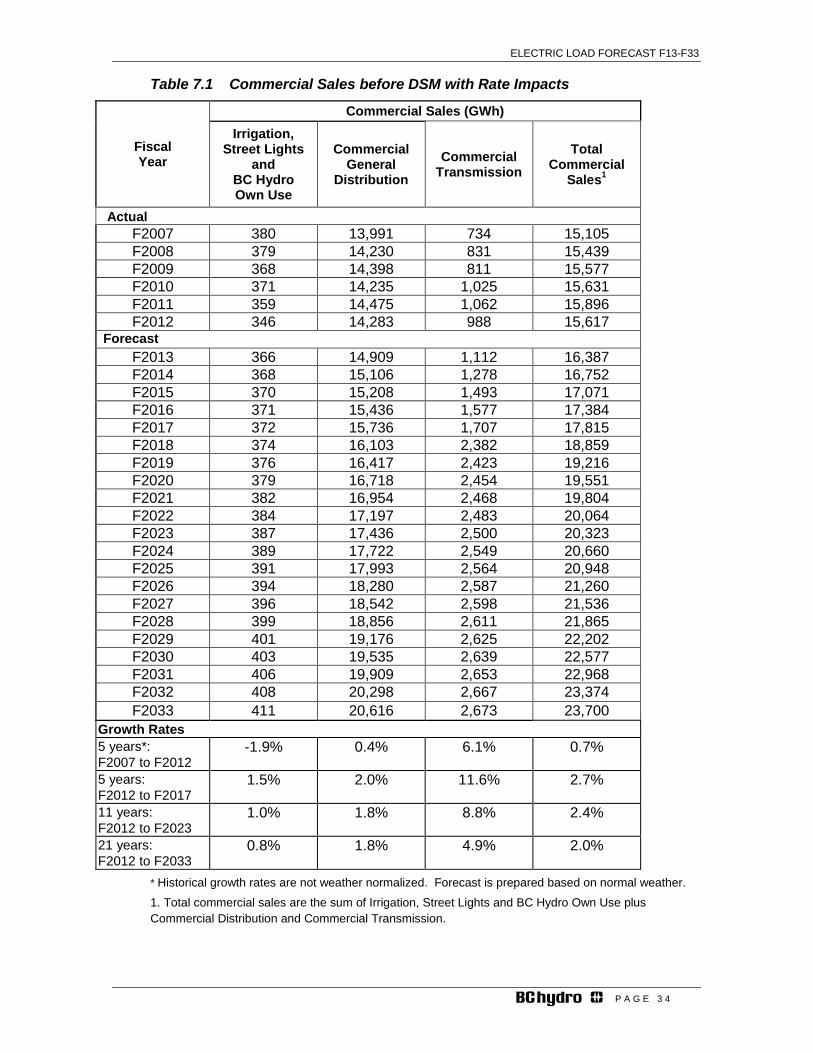
Figure 8.1 Comparison of Industrial Sales Forecast before DSM and Rate Impacts ...... 36
Figure 10.1 Comparison of BC Hydro’s Distribution Peak Demand Forecast before DSM with Rate Impacts ..................................................................................................... 56
Figure 10.2 Comparison of Transmission Peak Demand Forecast before DSM with Rate Impacts ..................................................................................................................... 58
Figure 10.3 Comparison of BC Hydro’s Integrated System Peak Demand Forecast before DSM with Rate Impacts ................................................................................. 60
Figure A1.1 Statistically Adjusted End Use (SAE) Model ................................................. 69
Figure A1.2 Peak Demand Forecast Roll-up ................................................................... 73
Figure A3.1: Oil and Gas Sector ...................................................................................... 82
Figure A3.1. Map of Montney and Horn River Basins ...................................................... 86
Figure A3.2 Montney Shale Gas Production Forecast ................................................... 91
Figure A3.3 Well Production Curve (with other industry projections) .............................. 91

ELECTRIC LOAD FORECAST F13-F33
P A G E 7
Executive Summary
Background and Context BC Hydro is the third largest utility in Canada and serves 95 percent of British Columbia’s population. BC Hydro’s total energy requirements, including losses and sales to other utilities and non-integrated areas (NIAs), were 57,083 GWh in F20121. Excluding the NIAs, the total integrated system energy requirements were 56,800 GWh2. The total integrated system peak demand in F2012 before weather adjustments and including losses and peak demand supplied by BC Hydro to other utilities was reported to be 10,338 MW excluding any load curtailments and outages. Load forecasting is central to BC Hydro’s long-term planning, medium-term investment, and short-term operational and forecasting activities. BC Hydro’s Electric Load Forecast is published annually for the purpose of providing decision-making information regarding “where, when and how much” electricity is expected to be required on the BC Hydro system. The forecast is based on several end-use and econometric models that use historical billed sales data up to March 31 of the relevant year, combined with a variety of economic forecasts and inputs from internal, government and third party sources. BC Hydro’s load forecasting activities are focused on the preparation of a number of term-specific and location-specific forecasts of energy sales and peak demand requirements in order to provide decision-making information for users. A variety of related products including monthly variance reports, inputs for revenue forecasts and load shape analyses, are produced to supplement the forecasts presented in this report.
Forecast Methodology BC Hydro produces 21-year forecasts (remainder of current year plus a 20 year projection) for both energy and peak demand. These forecasts are compiled separately but undergo a number of checks to ensure consistency. The load forecasts are prepared before and after incremental Demand Side Management (DSM). The load forecast presented in the Executive Summary and the remainder of the document is before incremental DSM. This is done to keep continuity with previous Annual Load Forecast documents and is consistent with the British Columbia Utilities Commission’s (BCUC) Resource Planning Guidelines. Load Forecasts with incremental DSM are presented in other documents such as BC Hydro’s Integrated Resource Plan (IRP) or Revenue Requirements Applications. BC Hydro incorporates relatively certain loads and demand trends into its load forecast. BC Hydro’s makes use of its Residential and Commercial End Use surveys to calibrate its end use models to historical trends in various end uses and space heating trends. Similarly, BC Hydro includes verifiable information regarding specific customer loads in its load forecast in order to reflect possible reductions due to customer attrition. BC Hydro is closely monitoring technological trends such as the future effects of electrification loads for possible inclusion into its base (Reference, which is the mid) load forecast. In terms of incremental electrification loads, demands from future electrical vehicle (EV) loads are included in the Reference load forecast. EV load estimates are lower as compared to the 2011 Load Forecast for the forecast period; EV load is estimated to be about 1,000 gigawatts per annum (GWh/year) towards the end of the 20 years. Other potential electrification loads are monitored for inclusion into the forecast. The impacts of possible future electricity rate increases (i.e. rate impacts) are also
1 BC Hydro’s fiscal year end is March 31; thus, F2012 covers April 1, 2011 to March 31, 2012. 2 The NIAs include the Purchase Areas, Zone II and Fort Nelson. A number of small communities located in the northern and southern areas of B.C. that are not connected to BC Hydro’s electrical grid make up the Purchase Areas and Zone II.

ELECTRIC LOAD FORECAST F13-F33
P A G E 8
reflected in BC Hydro’s load forecasts. Load forecasts presented in this document are designated as being ‘with rate impacts’ unless otherwise noted. The energy forecast is produced for each of the three major customer classes: residential, commercial and industrial. Sales to the three customer classes are combined with sales to other utilities to develop total BC Hydro firm sales. These sales estimates are adjusted for system line losses resulting in total gross energy requirements. To determine gross energy requirements for only the integrated system, sales and losses to all NIAs are excluded.
Residential The residential sector forecast is the product of accounts and use per account. The account forecast is driven by projections of regional housing starts. This sector is most responsive to variations in temperature relative to the other sectors. The residential use per account forecast (before Rates Impacts, electric vehicles and adjustments for codes and standards) are developed with Statistically Adjusted End-Use (SAE) models. These models combine traditional regression-based forecasting with detailed end-use data to produce forecasts. The key drivers of these end-use models are regional economic variables (i.e., disposable income and population, etc.) and non-economic variables such as weather and average stock efficiency of the various end uses of electricity. Commercial The total commercial sales forecast includes commercial general distribution loads, other commercial distribution loads such as irrigation and street lighting, and commercial transmission-connected loads such as pipelines and institutions such as universities. In terms of forecasting complexity, larger commercial accounts are forecast using similar methods for large industrial accounts. These methods are forward-looking information that includes expected sector trends, whereas the forecasts for the smaller sales categories such as street lighting rely upon historical sales trends. The commercial general distribution sales forecasts (before including Rates Impacts, electric vehicles and adjustments for codes and standards) are developed with SAE models. The key drivers of these end-use models are regional economic variables (i.e., commercial output (Gross Domestic Product (GDP)), employment, retail sales, and non-economic variables such as weather and average stock efficiency of the various end uses of electricity. Industrial
The industrial sector is made up of distribution and transmission-connected customers. The industrial distribution forecast is developed for specific sub-sectors; where sub-sector analysis has not undertaken, GDP growth projections are used to develop the forecast. The forecasts for larger transmission-connected industrial customers are primarily done on an individual customer account basis and sector basis, utilizing specific customer and sector expertise from inside and outside of BC Hydro (e.g., third party consultant studies). BC Hydro applies a risk assessment to specific accounts within each sector to quantify their individual contribution to a total system forecast. These assessments are based on industry and customer-specific risk factors such as commodity prices, and First Nations/environmental issues.
Forestry is made up of wood, pulp and paper and chemicals, where wood and pulp and paper are most of the sales. Mill specific information on production, intensity and on-site generation as well global outlooks for forestry products such as Kraft pulp, papers and packaging are used to develop the forestry forecast.

ELECTRIC LOAD FORECAST F13-F33
P A G E 9
For the mining sector, the forecast is developed using industrial sector reports from consultants, government mining reports, production forecasts and energy intensity factors. BC Hydro applies risk adjustments to mining project loads, which are intended to factor development risks. Some of the considerations that inform these weights include the financial viability of projects; the status of environmental approvals and whether or not the potential mine proponent has formally applied to BC Hydro for electrical service. For the oil and gas sector, BC Hydro employs two approaches to develop load forecasts, specifically the top-down and the bottom-up methodology. For the top-down approach, BC Hydro uses internal and third party predictions of oil and gas production and energy intensities to create annual load forecasts. The bottom-up method involves the development of forecasts of customer-specific loads, which are then risk adjusted and summed to produce composite loads. The risk adjustment factors are informed by discussions with BC Hydro’s key account managers, potential new customers, and government/industry experts. Future LNG Load To date, several Liquefied Natural Gas (LNG) proponents have approached BC Hydro and/or the B.C. Government with respect to LNG projects for the B.C. north coast.
Over the past couple of years, BC Hydro and government have been working with LNG proponents on options for meeting all or some of the energy needs of LNG plants with power from the BC Hydro system. The two key options available to LNG developers that involve BC Hydro providing electrical service include:
a) Provide power for entire plants with electricity. There is currently a single LNG plant in the world that uses electricity to power liquefaction compressors for making LNG.
b) Provide power under a hybrid approach. Natural gas would power liquefaction compressors — about 85 per cent of a plant’s energy needs — and BC Hydro would supply the rest of the plant’s needs.
The potential new demands of non-compression loads are material and could be between 800 GWh/year to 6,600 GWh/year of additional energy demand, corresponding to about 100 megawatts (MW) to 800 MW of additional peak demand. Given the materiality and binary nature of these outcomes, consideration of these loads in context of the load forecast and its impact of the supply and demand load resource balance will be addressed in BC Hydro’s long term plans (e.g., IRPs). Hence the 2012 Reference (mid) load forecast as presented in this document does not include potential LNG loads apart from very small allocations associated with on-site construction (for example, at its highest LNG on-site construction load is forecast to be 86 GWh in F2015). New gas processing and chilling demands from LNG facilities would significantly increase the requirements for electricity above BC Hydro’s mid load forecast as presented below. A range of LNG loads are considered as scenarios, and are addressed separately in BC Hydro’s planning process. Peak Demand A peak demand forecast is produced for each of BC Hydro’s distribution substations and for individual transmission customer accounts. Distribution substation forecasts are prepared for 15 distribution planning areas using energy forecasts and other drivers such as smaller distribution loads or spot loads. These substation forecasts are further aggregated on a coincident basis to develop a total system coincident distribution peak forecast. Relevant production and account information from the transmission energy forecast informs the peak forecasts for each of BC Hydro’s large transmission customers.
ELECTRIC LOAD FORECAST F13-F33
P A G E 1 0
The transmission peak forecasts for each account are aggregated on a coincident basis to develop a total system coincident transmission peak forecast. The total system peak forecast includes the system coincident distribution, transmission, peak demand transfers from BC Hydro to other utilities and system transmission losses.
Comparative Load Forecasts The 2012 Load Forecast was prepared in the fall of 2012 as part of BC Hydro’s annual forecasting cycle. The forecast methodology is similar to that used for the 2008 Load Forecast, which was reviewed by BCUC in the 2008 Long Term Acquisition Plan (LTAP) proceeding. The major changes in methodology since the 2008 Load Forecast include:
1. A portion of the industrial distribution sector is now forecast on a sub-sector basis (i.e., mining, oil and gas, wood) versus the previous use of a regression analysis for the entire sector. This change has enhanced the Load Forecast by improving upon the regional and total system load projections by incorporating load drivers such as the pine beetle infestation and specific industrial customer expansions;
2. EV load is now included in the 2012 (Reference) Load Forecast. The EV load estimates are moderate over the first 10 years of the forecast with 14 GWh projected for F2017. By F2032, the EV load rises to 1,270 GWh; and
3. The potential for DSM double counting issue was raised in the 2008 LTAP proceeding.3 Adjustments to the load forecast for DSM double counting were first made in the 2009 Load Forecast, and have been continued up to the current (2012) Load Forecasts. Appendix 5 shows the annual adjustments for the overlap in codes and standards.
As shown in the tables below at the total system level, the 2012 Load Forecast is below the 2011 Load Forecast for all years of the forecast for both energy and peak demand.
3 Refer to 2008 LTAP Decision, Directive 6, page 180. BC Hydro’s load forecasting models assume the U.S. Energy Information Administration’s (EIA) level of end-use efficiencies. These EIA efficiency levels form the basis of the double counting which results in a lower forecast. In addition, DSM savings due to codes and standards are subtracted in the Load Forecast.
ELECTRIC LOAD FORECAST F13-F33
P A G E 1 1
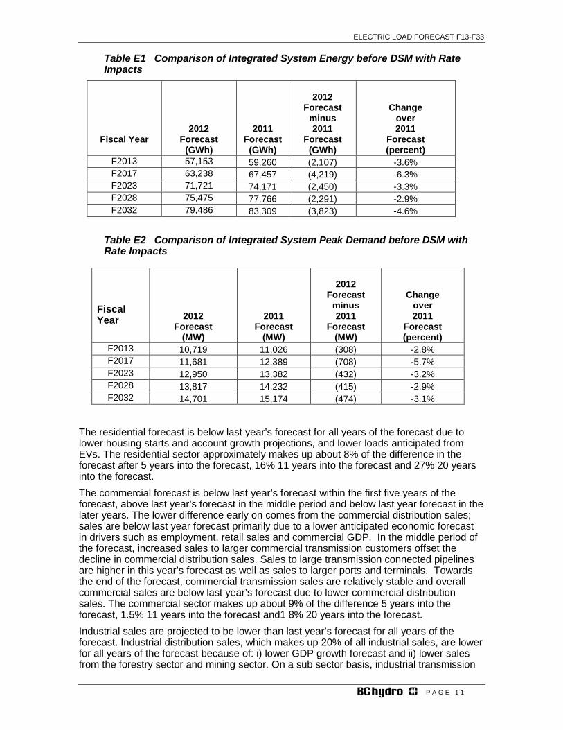
Table E1 Comparison of Integrated System Energy before DSM with Rate Impacts
Fiscal Year
2012 Forecast
(GWh)
2011 Forecast
(GWh)
2012 Forecast
minus 2011
Forecast (GWh)
Change over 2011
Forecast (percent)
F2013 57,153 59,260 (2,107) -3.6% F2017 63,238 67,457 (4,219) -6.3% F2023 71,721 74,171 (2,450) -3.3% F2028 75,475 77,766 (2,291) -2.9% F2032 79,486 83,309 (3,823) -4.6%
Table E2 Comparison of Integrated System Peak Demand before DSM with Rate Impacts
Fiscal Year
2012 Forecast
(MW)
2011 Forecast
(MW)
2012 Forecast
minus 2011
Forecast (MW)
Change over 2011
Forecast (percent)
F2013 10,719 11,026 (308) -2.8% F2017 11,681 12,389 (708) -5.7% F2023 12,950 13,382 (432) -3.2% F2028 13,817 14,232 (415) -2.9% F2032 14,701 15,174 (474) -3.1%
The residential forecast is below last year’s forecast for all years of the forecast due to lower housing starts and account growth projections, and lower loads anticipated from EVs. The residential sector approximately makes up about 8% of the difference in the forecast after 5 years into the forecast, 16% 11 years into the forecast and 27% 20 years into the forecast. The commercial forecast is below last year’s forecast within the first five years of the forecast, above last year’s forecast in the middle period and below last year forecast in the later years. The lower difference early on comes from the commercial distribution sales; sales are below last year forecast primarily due to a lower anticipated economic forecast in drivers such as employment, retail sales and commercial GDP. In the middle period of the forecast, increased sales to larger commercial transmission customers offset the decline in commercial distribution sales. Sales to large transmission connected pipelines are higher in this year’s forecast as well as sales to larger ports and terminals. Towards the end of the forecast, commercial transmission sales are relatively stable and overall commercial sales are below last year’s forecast due to lower commercial distribution sales. The commercial sector makes up about 9% of the difference 5 years into the forecast, 1.5% 11 years into the forecast and1 8% 20 years into the forecast. Industrial sales are projected to be lower than last year’s forecast for all years of the forecast. Industrial distribution sales, which makes up 20% of all industrial sales, are lower for all years of the forecast because of: i) lower GDP growth forecast and ii) lower sales from the forestry sector and mining sector. On a sub sector basis, industrial transmission

ELECTRIC LOAD FORECAST F13-F33
P A G E 1 2
sales have changed as follows: 1. Mining sales are lower due to deferred start-ups and reduced probabilities for new
mines driven by lower commodity price expectations and global uncertainty;
2. Sales to forestry are lower as a result of lower load expectations for several Kraft pulp mills and continued trends in digital substitution away from print media;
3. Other transmission sales are lower because of brief delays for expansions for some bulk terminals; and
4. Oil and gas over the short-term as natural gas prices are anticipated to be lower in the short term resulting from deferrals in drilling plans and activities.
Overall total industrial sales make up about 63% of the difference in the overall forecast 5 years into the forecast, 72% 11 years into the forecast and 45% 20 years into the forecast.
2012 Annual Sector and Peak Demand Forecasts
Residential Forecast Load in the residential sector, while subject to short-term variability due to weather events, tends to exhibit more predictable growth compared to the other sectors. The residential sector is forecast on a regional basis with the key forecast features including the following: • Electricity Use – BC Hydro’s residential sector currently consumes about 35 percent of
BC Hydro’s total annual firm billed sales. This electricity is used to provide a range of services (end uses) including space heating, water heating, refrigeration, and miscellaneous plug-in load which includes computer equipment and home entertainment systems.
• Drivers – The drivers of the residential forecast are number of accounts and the average annual use per account. Growth in the total number of accounts is driven largely by growth in housing starts. The use per account forecast is developed on a regional basis from the SAE models. The drivers of the model include economic variables such as disposable income, weather and average stock efficiency of residential end uses of electricity.
• Trends – The residential sales forecast is below the 2011 Load Forecast for all years of the forecast primarily from lower predicted housing starts growth and therefore accounts growth is expected to be slower relative to the previous forecast. The energy impact of EVs over the long term is considerably lower than the 2011 forecast reflecting revised drivers of the EV load model. The 21-year compound growth rate4, before DSM and with Rate Impacts, is projected to be 1.8 percent per annum.
Refer to Chapter 6 for a detailed description of the residential forecast.
Commercial Forecast BC Hydro’s commercial sector encompasses a wide variety of commercial and publicly-provided services, including irrigation, street lighting and BC Hydro’s own use. The most diverse commercial segment consists of customers who operate a range of facilities such as office buildings, retail stores and institutions (i.e., hospitals and schools) provided at distribution voltages. It also includes transportation facilities in the form of pipelines and bulk transportation terminals which receive electricity at transmission voltages. The key features of the commercial forecast include the following:
4 Unless otherwise noted, all growth rates are calculated as annual compound growth rates.

ELECTRIC LOAD FORECAST F13-F33
P A G E 1 3
• Electricity Use – BC Hydro’s commercial sector currently consumes 30 percent of BC Hydro’s total annual firm billed sales. On the distribution system, electricity is used to provide a range of services such as lighting, ventilation, heating, cooling, refrigeration and hot water. These needs vary considerably between different types of buildings and types of loads.
• Drivers – Consumption in commercial distribution sales is closely tied with economic activity in the province. Key drivers for the commercial distribution sales include retail sales, employment and commercial output. Other drivers of the end use forecasting model for this sector include weather and commercial end use stock average efficiency forecasts. For the commercial transmission sector, individual customer load projections are developed. Historical load trends are a good indicator of future trends for accounts with relatively stable loads.
• Trends – Electricity consumption in the commercial sector can vary considerably from year to year, reflecting the level of activity in B.C.’s service sector. Total commercial forecast is below the 2011 Forecast in the initial period of the forecast; this primarily reflects lower commercial distribution sales driven by slower growing economic drivers. Towards the middle the forecast, the 2012 Forecast is above 2011 Forecast as stronger sales to large pipelines are expected. Total commercial sales towards the end of the forecast are projected to be below last year’s forecast due to lower EV load expectations and a lower long term economic growth projection. Over a 21-year period, the 2012 Load Forecast growth rate, before DSM and with Rate Impacts, is 2.0 percent per annum.
• Refer to Chapter 7 for a detailed description of the commercial forecast. Industrial Forecast BC Hydro’s industrial sector is concentrated in a limited number of industries, the most important of which are pulp and paper, wood products, chemicals, metal mining, coal mining and oil and gas sector loads. The remaining industrial load is made up of a large number of small and medium sized manufacturing establishments. Key features of the industrial forecast include the following: • Electricity Use – BC Hydro’s industrial sector currently consumes 32 percent of
BC Hydro’s total annual firm billed sales. This electricity is used in a variety of applications including fans, pumps, compression, conveyance, processes such as cutting, grinding, stamping and welding and electrolysis. At distribution voltages, wood products manufacturing is the major component of industrial sales.
• Drivers – Industrial electricity consumption is tied closely with economic conditions in the province, and the broader export markets, product commodity prices, and world and domestic events that impact product demand. The key drivers of the forecasts are production, intensity levels, third party industry reports and changes in customer plant operations as identified by BC Hydro’s Key Account Managers. Probability assessments are undertaken for existing accounts and new accounts to determine specific customer load projections.
• Trends – Electricity consumption in the industrial sector is quite volatile, driven substantially by external economic conditions that affect commodity markets. The current forecast is lower for all years of the forecast. This reflects several factors such as deferrals and lower probabilities for mining loads, less sales expected for Kraft pulp mills, lower wood sector sales due to slower recovery of US housing starts and reduced gas producer loads in the short term as drilling activity has been pushed back. The 21-year growth rate in the current forecast, before DSM and with Rate Impacts is 1.3 percent per annum.
Refer to Chapter 8 for a detailed description of the industrial forecast.
ELECTRIC LOAD FORECAST F13-F33
P A G E 1 4
Peak Demand Peak demand is composed of the demand for electricity at the distribution level, transmission level plus inter-utility transfers and transmission losses on the integrated system. Key features of the peak forecast include the following: • Electricity Use – Peak demand is forecast as the maximum expected one-hour
demand during the year. For BC Hydro’s load, this event occurs in the winter with the peak driven particularly by space heating load. As with the 2011 Load Forecast, BC Hydro’s peak forecast is based on normalized weather conditions, which is the rolling average of the coldest daily average temperature over the most recent 30 years.
• Drivers – Key drivers of electricity peak include the level of economic activity, number of accounts, employment and the other discrete developments such as new shopping malls, waste treatment plants or industrial facilities that drive substation peak demand.
• Trends – BC Hydro’s total system peak forecast has grown moderately over the past couple of years. Slower economic growth has tempered increases in distribution and transmission peak demand. The current total system peak forecast is below the 2011 Forecast for all years of the forecast. This is due to lower housing starts and residential account growth projection, slower growth in economic variables such as employment, retails sales and GDP, and lower peak demand from larger industrial customers. The 21-year growth rate in the current forecast, before DSM and with Rate Impacts is 1.8 percent per annum.
• Refer to Chapter 10 for a detailed description of the peak demand forecast Similar to the 2011 Load Forecast, the energy and peak demand requirements for unconventional gas producers within the Horn River Basin are not included in the 2012 Reference load projections for Fort Nelson. BC Hydro has constructed scenarios that examine various Horn River shale gas play load requirements and alternatives on how to supply these loads. These scenarios are examined in BC Hydro’s IRP.
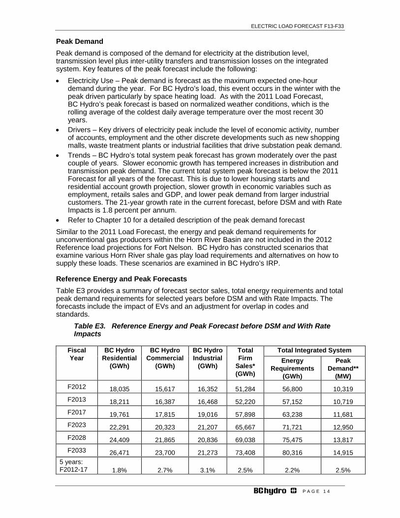
Reference Energy and Peak Forecasts Table E3 provides a summary of forecast sector sales, total energy requirements and total peak demand requirements for selected years before DSM and with Rate Impacts. The forecasts include the impact of EVs and an adjustment for overlap in codes and standards.
Table E3. Reference Energy and Peak Forecast before DSM and With Rate Impacts
Fiscal Year
BC Hydro Residential
(GWh)
BC Hydro Commercial
(GWh)
BC Hydro Industrial
(GWh)
Total Firm
Sales* (GWh)
Total Integrated System Energy
Requirements (GWh)
Peak Demand**
(MW) F2012 18,035 15,617 16,352 51,284 56,800 10,319 F2013 18,211 16,387 16,468 52,220 57,152 10,719 F2017 19,761 17,815 19,016 57,898 63,238 11,681 F2023 22,291 20,323 21,207 65,667 71,721 12,950 F2028 24,409 21,865 20,836 69,038 75,475 13,817 F2033 26,471 23,700 21,273 73,408 80,316 14,915
5 years: F2012-17 1.8% 2.7% 3.1% 2.5% 2.2% 2.5%

ELECTRIC LOAD FORECAST F13-F33
P A G E 1 5
11 years: F2012-23 1.9% 2.4% 2.4% 2.3% 2.1% 2.1% 21 years: F2012-33 1.8% 2.0% 1.3% 1.7% 1.7% 1.8%
* Total firm sales includes sales to all residential, commercial and industrial customers and sales to all other utilities including Seattle City Light, City of New Westminster and FortisBC and Hyder.
** Peak Demand for F2012 is weather normalized as shown in the table.
ELECTRIC LOAD FORECAST F13-F33
P A G E 1 6
1 Introduction
BC Hydro's Load Forecast is typically published annually. The Load Forecast consists of a 21-year forecast (remainder of the current year plus a 20-year projection) for future energy and peak demand requirements. These forecasts focus on the annual Reference Load Forecast or the most likely electricity demand projections that are used for planning future energy and peak supply requirements.
The Load Forecast is used to provide decision-making support for several aspects of BC Hydro’s business including: the Integrated Resource Plan, revenue requirements, rate design, system planning and operations and the Service Plan.
Ranges in the load forecasts, referred to as uncertainty bands, are developed using simulation methods. These bands represent the expected ranges around the annual Reference load forecasts at certainty levels of statistical confidence. These forecasts are produced because there is uncertainty in the variables that predict future loads and in the predictive powers of the forecasting models.
The Reference energy forecast consists of a sales forecast for three main customer sectors (residential, commercial and industrial) plus the other utilities supplied by BC Hydro. The Reference Total Gross energy requirements forecast consists of the sector sales forecast, other utility sales forecast plus total line losses.
The sales forecast is developed by analyzing and modeling the relationships between energy sales and the predictors of future sales, which are referred as forecast drivers. Drivers consist of both economic variables and non-economic variables. Economic variables include GDP, housing starts, retail sales, employment and electricity prices (rates). Non-economic variables include weather and average stock efficiency of various residential and commercial end uses of electricity.
The Rate Impacts are reflected in the Reference forecasts; these impacts consist of the effect on load due to potential electricity rate changes under flat rate structures or a single tier rate design5. Savings or reductions in the load due to changes in rate structures are considered to be part of BC Hydro’s 20-year DSM Plan. These savings are not included in the load forecasts contained in this document but are contained in other applications such as BC Hydro’s Revenue Requirements Application.
The total Reference peak forecast consists of peak demands for BC Hydro’s coincident distribution substations, large transmission-connected customers and other utilities, along with total transmission losses. The distribution peak demand forecast is developed by analyzing and modelling the relationship between aggregate substation peak demands and economic variables. Distribution peak forecasts are prepared under average cold weather conditions or a design temperature. The transmission peak demand is based on estimating the future demands of larger customers which are driven by future market conditions and company-specific production plans.
BC Hydro continuously attempts to improve the accuracy of its forecasting process by monitoring trends in forecasting approaches and tracking developments that may affect the load forecasts. Forecasts are continually monitored and compared to sales, and are adjusted for variances. Additionally, the load forecasts are adjusted if new information on forecast drivers becomes available during the year they are developed.
5 The electricity price elasticity of demand used to develop the rate impacts is assumed to be -0.05 for all rate classes. Additional rate-induced savings resulting from stepped rates (conservation rates) are counted separately as DSM savings.

ELECTRIC LOAD FORECAST F13-F33
P A G E 1 7
For continuity between the 2011 Load Forecast and the 2012 Forecast, load estimates of EVs are shown in Appendix 4, and adjustment for double counting in codes and standards is shown in Appendix 5. These load categories are necessarily included in the Reference load forecast.
Comparisons between the 2011 and the 2012 Forecasts for the Residential and Commercial section are with rate impacts. The Industrial section is compared before rate impacts so as to highlight the key differences between the two vintages of forecasts. The 2012 large industrial transmission loads do not include any LNG loads. These loads are considered in separate load scenarios in BC Hydro’s planning process.

ELECTRIC LOAD FORECAST F13-F33
P A G E 1 8
2 Regulatory Background and Current Initiatives The British Columbia Utilities Commission (BCUC), various intervenors and other stakeholders have reviewed BC Hydro’s Electric Load Forecasts in past years by way of the following regulatory review processes: • 2003 Vancouver Island Generation Project – Certificate of Public Convenience and
Necessity (CPCN) Application • F2005 and F2006 Revenue Requirements Application (RRA) • 2004 Vancouver Island Call for Tenders – Electricity Purchase Agreement (EPA) • F2006 Call for Tenders • F2007 and F2008 RRA • 2006 Integrated Electricity Plan (IEP) and Long Term Acquisition Plan (LTAP) • 2008 LTAP • F2009 and F2010 RRA • 2009 Waneta Transaction • F2011 RRA • F2012-F2014 RRA (Order G-77-12A June 20, 2012) • Dawson Creek/Chetwynd Area Transmission (DCAT) Project. (Decision October
10, 2012) During F2012, there were no major directives that impact the development of the 2012 Forecast from the most recent Decisions and Orders noted above. In its decision on the 2008 LTAP, the BCUC issued two directives related to the 2008 Load Forecast. BC Hydro’s 2010 Annual Load Forecast document addresses these two directives in detail. At this time, BC Hydro believes that there is no additional work required to fulfill Directive 7. As for Directive 6 which centers issues related to DSM/Load integration BC Hydro has continued its work in this area and made adjustments to its current load forecast to account for potential overlap between the Load Forecast and the DSM Plan estimates for codes and standards. Please see Appendix 5 for further details on the adjustments.
ELECTRIC LOAD FORECAST F13-F33
P A G E 1 9
3 Forecast Drivers, Data Sources and Assumptions
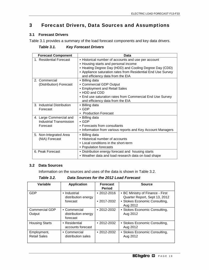
3.1 Forecast Drivers Table 3.1 provides a summary of the load forecast components and key data drivers.
Table 3.1. Key Forecast Drivers
Forecast Component Data 1. Residential Forecast • Historical number of accounts and use per account
• Housing starts and personal income • Heating Degree Day (HDD) and Cooling Degree Day (CDD) • Appliance saturation rates from Residential End Use Survey
and efficiency data from the EIA 2. Commercial
(Distribution) Forecast • Billing data • Commercial GDP Output • Employment and Retail Sales • HDD and CDD • End use saturation rates from Commercial End Use Survey
and efficiency data from the EIA 3. Industrial Distribution
Forecast • Billing data • GDP • Production Forecast
4. Large Commercial and Industrial Transmission Forecast
• Billing data • GDP • Forecasts from consultants • Information from various reports and Key Account Managers
5. Non-Integrated Area (NIA) Forecast
• Billing data • Historical number of accounts • Local conditions in the short-term • Population forecasts
6. Peak Forecast • Distribution energy forecast and housing starts • Weather data and load research data on load shape
3.2 Data Sources Information on the sources and uses of the data is shown in Table 3.2. Table 3.2. Data Sources for the 2012 Load Forecast
Variable Application Forecast Period
Source
GDP • Industrial distribution energy forecast
• 2012-2016 • 2017-2032
• BC Ministry of Finance - First Quarter Report, Sept 13, 2012
• Stokes Economic Consulting, Aug 2012
Commercial GDP Output
• Commercial distribution energy forecast
• 2012-2032 • Stokes Economic Consulting, Aug 2012
Housing Starts • Residential accounts forecast
• 2012-2032 • Stokes Economic Consulting, Aug 2012
Employment, Retail Sales
• Commercial distribution sales
• 2012-2032
• Stokes Economic Consulting, Aug 2012
ELECTRIC LOAD FORECAST F13-F33
P A G E 2 0
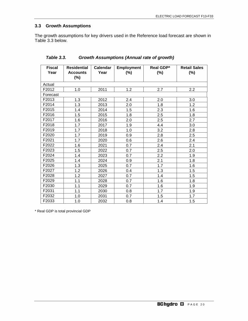
3.3 Growth Assumptions
The growth assumptions for key drivers used in the Reference load forecast are shown in Table 3.3 below.
Table 3.3. Growth Assumptions (Annual rate of growth)
Fiscal Year
Residential Accounts
(%)
Calendar Year
Employment (%)
Real GDP* (%)
Retail Sales (%)
Actual F2012 1.0 2011 1.2 2.7 2.2 Forecast F2013 1.3 2012 2.4 2.0 3.0 F2014 1.3 2013 2.0 1.8 1.2 F2015 1.4 2014 1.5 2.3 1.6 F2016 1.5 2015 1.8 2.5 1.8 F2017 1.6 2016 2.0 2.5 2.7 F2018 1.7 2017 1.9 4.4 3.0 F2019 1.7 2018 1.0 3.2 2.8 F2020 1.7 2019 0.9 2.8 2.5 F2021 1.7 2020 0.6 2.6 2.4 F2022 1.6 2021 0.7 2.4 2.1 F2023 1.5 2022 0.7 2.5 2.0 F2024 1.4 2023 0.7 2.2 1.9 F2025 1.4 2024 0.9 2.1 1.8 F2026 1.3 2025 0.7 1.7 1.6 F2027 1.2 2026 0.4 1.3 1.5 F2028 1.2 2027 0.7 1.4 1.5 F2029 1.1 2028 0.7 1.6 1.8 F2030 1.1 2029 0.7 1.6 1.9 F2031 1.1 2030 0.8 1.7 1.9 F2032 1.0 2031 0.7 1.5 1.7 F2033 1.0 2032 0.8 1.4 1.5
* Real GDP is total provincial GDP
ELECTRIC LOAD FORECAST F13-F33
P A G E 2 1
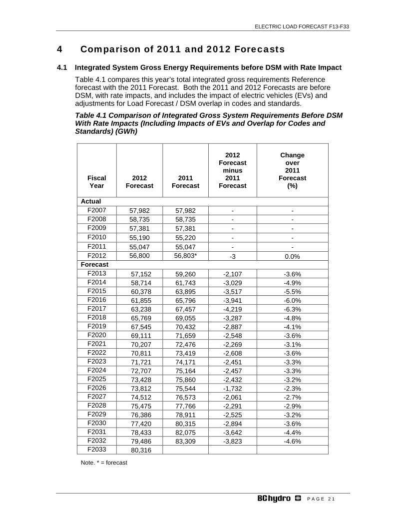
4 Comparison of 2011 and 2012 Forecasts
4.1 Integrated System Gross Energy Requirements before DSM with Rate Impact Table 4.1 compares this year’s total integrated gross requirements Reference forecast with the 2011 Forecast. Both the 2011 and 2012 Forecasts are before DSM, with rate impacts, and includes the impact of electric vehicles (EVs) and adjustments for Load Forecast / DSM overlap in codes and standards. Table 4.1 Comparison of Integrated Gross System Requirements Before DSM With Rate Impacts (Including Impacts of EVs and Overlap for Codes and Standards) (GWh)
Fiscal Year
2012 Forecast
2011 Forecast
2012
Forecast minus 2011
Forecast
Change
over 2011
Forecast (%)
Actual F2007 57,982 57,982 - - F2008 58,735 58,735 - - F2009 57,381 57,381 - - F2010 55,190 55,220 - - F2011 55,047 55,047 - - F2012 56,800 56,803* -3 0.0%
Forecast F2013 57,152 59,260 -2,107 -3.6% F2014 58,714 61,743 -3,029 -4.9% F2015 60,378 63,895 -3,517 -5.5% F2016 61,855 65,796 -3,941 -6.0% F2017 63,238 67,457 -4,219 -6.3% F2018 65,769 69,055 -3,287 -4.8% F2019 67,545 70,432 -2,887 -4.1% F2020 69,111 71,659 -2,548 -3.6% F2021 70,207 72,476 -2,269 -3.1% F2022 70,811 73,419 -2,608 -3.6% F2023 71,721 74,171 -2,451 -3.3% F2024 72,707 75,164 -2,457 -3.3% F2025 73,428 75,860 -2,432 -3.2% F2026 73,812 75,544 -1,732 -2.3% F2027 74,512 76,573 -2,061 -2.7% F2028 75,475 77,766 -2,291 -2.9% F2029 76,386 78,911 -2,525 -3.2% F2030 77,420 80,315 -2,894 -3.6% F2031 78,433 82,075 -3,642 -4.4% F2032 79,486 83,309 -3,823 -4.6% F2033 80,316
Note. * = forecast
ELECTRIC LOAD FORECAST F13-F33
P A G E 2 2
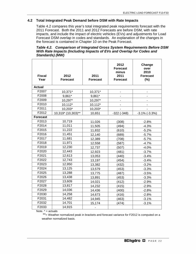
4.2 Total Integrated Peak Demand before DSM with Rate Impacts Table 4.2 compares this year’s total integrated peak requirements forecast with the 2011 Forecast. Both the 2011 and 2012 Forecasts are before DSM, with rate impacts, and include the impact of electric vehicles (EVs) and adjustments for Load Forecast DSM overlap in codes and standards. An explanation of the changes in the forecast is contained in Chapter 10 on the Peak Forecast. Table 4.2. Comparison of Integrated Gross System Requirements Before DSM With Rate Impacts (Including Impacts of EVs and Overlap for Codes and Standards) (MW)
Fiscal Year
2012 Forecast
2011 Forecast
2012
Forecast minus 2011
Forecast
Change
over 2010
Forecast (%)
Actual F2007 10,371* 10,371* - - F2008 9,861* 9,861* - - F2009 10,297* 10,297* - - F2010 10,112* 10,112* - - F2011 10,203* 10,203* - - F2012 10,319* (10,303)** 10,651 -322 (-348) -3.1% (-3.3%)
Forecast F2013 10,719 11,026 (308) -2.8% F2014 11,011 11,505 (494) -4.3% F2015 11,222 11,832 (610) -5.2% F2016 11,451 12,140 (689) -5.7% F2017 11,681 12,389 (708) -5.7% F2018 11,971 12,558 (587) -4.7% F2019 12,230 12,737 (507) -4.0% F2020 12,443 12,923 (481) -3.7% F2021 12,613 13,053 (440) -3.4% F2022 12,743 13,197 (454) -3.4% F2023 12,950 13,382 (432) -3.2% F2024 13,125 13,579 (453) -3.3% F2025 13,288 13,775 (487) -3.5% F2026 13,438 13,891 (453) -3.3% F2027 13,609 14,021 (412) -2.9% F2028 13,817 14,232 (415) -2.9% F2029 14,036 14,436 (400) -2.8% F2030 14,258 14,673 (416) -2.8% F2031 14,482 14,945 (463) -3.1% F2032 14,701 15,174 (474) -3.1% F2033 14,915 -
Note. * = actuals **= Weather normalized peak in brackets and forecast variance for F2012 is computed on a weather normalized basis.

ELECTRIC LOAD FORECAST F13-F33
P A G E 2 3
5 Sensitivity Analysis
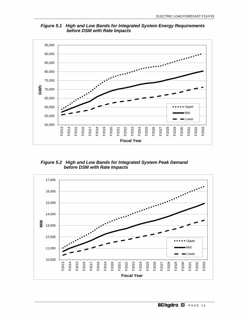
5.1 Background Future electricity consumption is fundamentally uncertain and dependent on many variables such as economic activity, weather, electricity rates and DSM. The future impact of these variables on load is characterized by significant uncertainty. Moreover, load is affected by extraordinary events such as strikes, trade disputes, pine beetle infestations and volatility in commodity markets. Additionally, world events such as recent economic crises, wars and revolutions impact electricity demand. BC Hydro tries to quantify the uncertainty in future load as much as possible by developing accurate, reliable and stable models that specify the relationship between load and its key drivers, and by using reliable and credible sources for forecasts of the key drivers of load. BC Hydro uses a Monte Carlo model to estimate the potential distribution of future loads, and to represent this against the Reference load forecast (see Appendix 2 for details on the Monte Carlo model). This model produces high and low uncertainty bands for each customer category around the Reference forecast by examining the impact on load from the uncertainty in a set of key drivers. For the industrial sector high and low uncertainty bands are generated by a discrete Low and High forecast of the four main industrial sectors (Forestry, Mining, Oil and Gas, and other). Uncertainty for electricity rates and response to electricity rate changes (price elasticity) are also considered in the overall high and low industrial uncertainty bands. For the residential and small commercial sectors, high and low uncertainty bands are generated from the Monte Carlo model using the following major causal factors: economic growth rate (measured by GDP), the electricity rates charged by BC Hydro to its customers, the sales response to electricity rate changes (price elasticity) and weather (reflected by heating degree-days). Probability distributions are assigned to each of these major causal factors, and a further distribution is assigned to a residual uncertainty variable which is also included in the Monte Carlo model. As with the 2011 Forecast, BC Hydro added to the Monte Carlo model a probability distribution for electric vehicles (EVs) and DSM/ load forecast integration on overlap of codes and standards. The Monte Carlo model uses simulation methods to quantify and combine the probability distributions, reflecting the relationships between all factors and electricity consumption with a correlation factor between the Residential, Commercial and Industrial loads. A probability distribution for the overall load forecast (i.e. total Gross Requirements) is thus obtained which shows the likelihood of various total load levels resulting from the simultaneous combined effect of all factors. The intention of this analysis is the creation of high and low forecast bands with approximately 10% and 90% exceedance probabilities, respectively. For planning purposes, BC Hydro uses its mid-load forecast. The high and low forecast bands are used to provide an indication of the magnitude of load uncertainty. The high and low load forecasts before DSM with rate impacts (excluding LNG Load) are shown in Figures 5.1 and 5.2. The high and low total peak forecasts contained in these tables are based on applying a load factor to Monte Carlo simulation outcomes of the total energy requirements.
ELECTRIC LOAD FORECAST F13-F33
P A G E 2 4
Figure 5.1 High and Low Bands for Integrated System Energy Requirements before DSM with Rate Impacts
Figure 5.2 High and Low Bands for Integrated System Peak Demand
before DSM with Rate Impacts
10,000
11,000
12,000
13,000
14,000
15,000
16,000
17,000
F201
3
F201
4
F201
5
F201
6
F201
7
F201
8
F201
9
F202
0
F202
1
F202
2
F202
3
F202
4
F202
5
F202
6
F202
7
F202
8
F202
9
F203
0
F203
1
F203
2
F203
3
MW
Fiscal Year
Upper
Mid
Lower
50,000
55,000
60,000
65,000
70,000
75,000
80,000
85,000
90,000
95,000
F201
3
F201
4
F201
5
F201
6
F201
7
F201
8
F201
9
F202
0
F202
1
F202
2
F202
3
F202
4
F202
5
F202
6
F202
7
F202
8
F202
9
F203
0
F203
1
F203
2
F203
3
GW
h
Fiscal Year
Upper
Mid
Lower

ELECTRIC LOAD FORECAST F13-F33
P A G E 2 5
6. Residential Forecast
6.1. Sector Description The residential sector currently comprises about 35% of BC Hydro’s total annual sales. This electricity is used to provide a range of services for customers (referred to as “end-uses”). Examples of residential end-uses of electricity are space heating, water heating, refrigeration, and miscellaneous plug-in loads which include computer equipment and home entertainment systems. Since space and water heating loads are dependent on the outside temperature, residential sales can be strongly affected by the weather. Of the 1.67 million residential accounts served by BC Hydro at the end of F2012, 58% are located in the Lower Mainland, 21% are on Vancouver Island, 13% are in the South Interior, and 8% are in the Northern Region. With regard to residential sales, 53% occur in the Lower Mainland, 26% on Vancouver Island, 13% in the South Interior and 8% in the Northern Region.
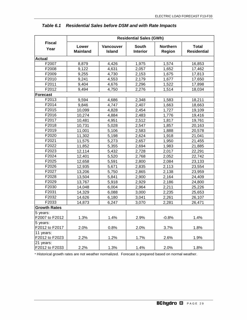
6.2 Forecast Summary Of the three major customer classes, apart from short-term weather impacts, the residential sector is the most stable in terms of demand variability. Sales to the residential sector are driven by two main factors – accounts and use per account. Growth in the number of residential accounts has been 1.6 percent per annum over the last 10 years. The annual growth rate in the number of accounts is expected to remain at 1.4 percent over the next 21 years. Growth in accounts is expected be strong the near and middle terms of the forecast period due to the significant investment expected to take place in the province. Historical use per account reflects several factors such as the recent lingering recession, efficiency-related modifications to building standards, and changes in appliance efficiency and BC Hydro’s DSM efforts. The forecast in use per account is expected to grow (before rate impacts and adjustments) on an average annual basis of 0.2 percent over the 20-year forecast period. The residential load forecast is shown in Table 6.1, including a breakdown by the four main regions. The average annual growth in residential sales over the entire forecast period is expected to be about 400 GWh per annum, including rate impacts and the adjustments for electric vehicles and the Load Forecast/DSM overlap for codes and standards.
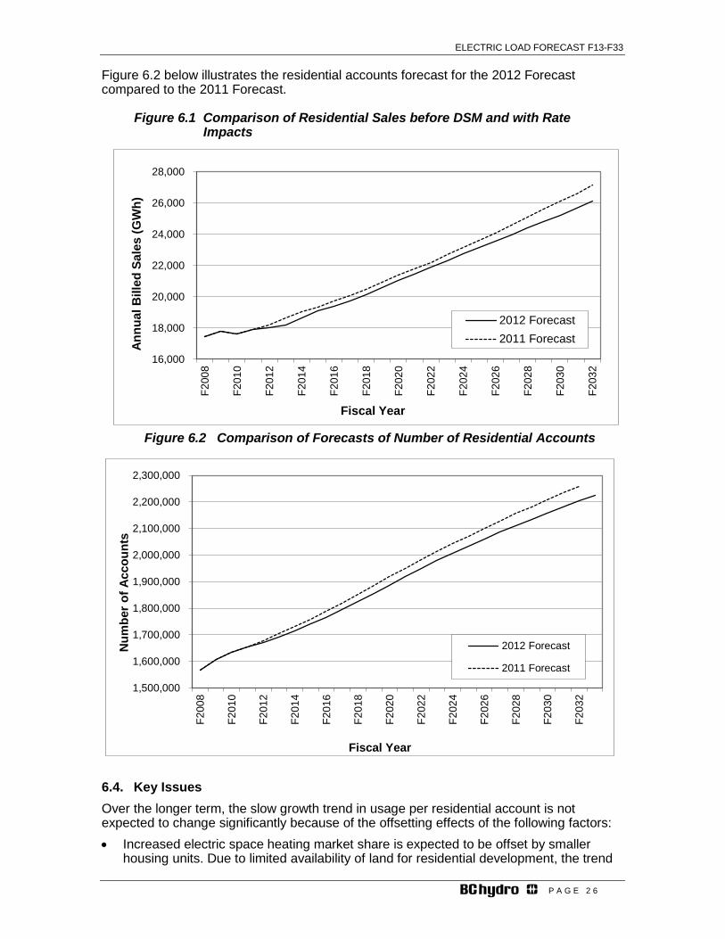
6.3 Residential Forecast Comparison Residential sales in the 2012 Forecast are projected to be lower than the 2011 Forecast over the entire forecast period (see Figure 6.1). Before DSM with rate impacts the decrease in the residential sales forecast is 440 GWh (-2.4%) in F2013, 327 GWh (-1.7%) in F2017, 399 GWh (-1.8%) in F2023 and 1,043 GWh (-3.8%) in F2032. The key variables that account for the lower residential sales are the residential accounts forecast and electrical vehicle loads projections. The ending number of accounts for F2012 was 1,671,358 which is 7,584 accounts (or 0.5%) below the level assumed in the 2011 Forecast. The lower starting point for the number of accounts and projections for housing starts are the main reasons why the total residential accounts forecast has been reduced. In the 2011 Forecast, the 5, 11, and 21-year growth rates for number of accounts were 1.6%, 1.7%, and 1.5% respectively. In the 2012 Forecast, the growth rates for number of accounts are 1.4%, 1.5% and 1.4%, respectively.
ELECTRIC LOAD FORECAST F13-F33
P A G E 2 6
Figure 6.2 below illustrates the residential accounts forecast for the 2012 Forecast compared to the 2011 Forecast.
Figure 6.1 Comparison of Residential Sales before DSM and with Rate Impacts
Figure 6.2 Comparison of Forecasts of Number of Residential Accounts
6.4. Key Issues Over the longer term, the slow growth trend in usage per residential account is not expected to change significantly because of the offsetting effects of the following factors: • Increased electric space heating market share is expected to be offset by smaller
housing units. Due to limited availability of land for residential development, the trend
1,500,000
1,600,000
1,700,000
1,800,000
1,900,000
2,000,000
2,100,000
2,200,000
2,300,000
F200
8
F201
0
F201
2
F201
4
F201
6
F201
8
F202
0
F202
2
F202
4
F202
6
F202
8
F203
0
F203
2
Num
ber o
f Acc
ount
s
Fiscal Year
2012 Forecast
2011 Forecast
16,000
18,000
20,000
22,000
24,000
26,000
28,000
F200
8
F201
0
F201
2
F201
4
F201
6
F201
8
F202
0
F202
2
F202
4
F202
6
F202
8
F203
0
F203
2
Annu
al B
illed
Sal
es (G
Wh)
Fiscal Year
2012 Forecast2011 Forecast

ELECTRIC LOAD FORECAST F13-F33
P A G E 2 7
in metropolitan centres is expected to be towards denser housing. Since row houses and apartments are more likely to be built with electric heat compared to single family homes, the market share for electrically-heated housing is expected to increase. Although new row houses and apartments tend to be larger than existing similar dwellings, they generally have a smaller floor area than detached single family homes, and therefore have lower space heating load requirements. The increase in market share of electric space heating is also offset to some extent by the improvements in building standards.
• Manufacturers throughout Canada and the U.S. are expected to continue to improve the energy efficiency of major electrical appliances. As older models wear out and are replaced by newer ones, electricity consumption for major appliances such as refrigerators, freezers, ovens and ranges is forecast to decrease. However, the new models of these appliances tend to be larger and include more features than models currently in use. Therefore, some of the reduction in electricity use resulting from improvements in electricity efficiency will be offset by increases in appliance size and extra features.
• The projected decrease in the number of people per household tends to reduce electricity use per account. However, this reduction is expected to be offset by changes to lifestyle and technological improvements, which are expected to cause an increase in demand for electronic, entertainment and telecommunication devices in the home. A trend towards home offices is also expected to produce a long-term increase in residential electricity consumption.
In the long term, the expected overall impact of these various trends is that the factors working to increase use rates will be offset by the factors working to decrease use rates.
6.5 Forecast Methodology The forecast for residential sales is calculated as the product of the forecast number of accounts times the forecast use per account. To develop the overall residential sales forecast, BC Hydro’s total service area was divided into four customer service regions – Lower Mainland, Vancouver Island, South Interior and Northern Region. For each region, a third party housing stock forecast was prepared based on the housing starts forecast in the region. The 2012 residential load forecast was prepared using the Statistically Adjusted End-Use (SAE) model. Refer to Appendix 1.1 for further details on the residential sales methodology and drivers of the SAE model.
6.6 Risks and Uncertainties Uncertainty in the residential sales forecast is due to uncertainty in three factors: forecast of number of accounts, forecast of use per account, and weather. (a) Number of Accounts: In the short term, an error in the forecast for account growth
would not result in a significant error in the forecast for total number of accounts. This is because account growth is on average 1.4% per year, so in the first year, an error of 1% in the forecast for account growth would result in an error of about 0.014% to the forecast for total number of accounts. However, in the long term, there is increased risk due to the cumulative effect of errors in the forecast for account growth.
(b) Use per Account: Most of the risk in the residential forecast resides in the forecast of use per account for the following reasons:
i. Unlike the forecast of account growth, an error of 1% in the forecast for use per account in any year would contribute to a direct error of 1% to the forecast for residential sales for that year.

ELECTRIC LOAD FORECAST F13-F33
P A G E 2 8
ii. The forecast for use per account is the net result of many counteracting factors. Some of the forces working to increase use rate are: • increases in home sizes; • natural gas prices increasing faster than electricity prices; • increases in electric space heating share; • increases in real disposable income; and • increases in saturation levels for appliances Some of the forces working to decrease use rate are: • increases in heating system efficiencies; • electricity prices increasing faster than natural gas prices; • new dwellings being built with higher insulation standards; • heat omissions from additional appliances reducing electric heating load; • increased use of programmable thermostats; and • decreases in household sizes
Although these positive and negative forces were recognized when the forecast for use rate was developed, there is uncertainty inherent in all of these factors.
(c) Weather: In the short term, weather is highly variable. Therefore, in any one year, there is a risk that weather may have a significant impact on residential sales. For example, the El Nino event of F1998 is estimated to have reduced residential sales by about 4%. Since average weather is expected to be close to the rolling 10-year normal values used in the 2012 Forecast, weather is not viewed as being a high risk to the long-term forecast for residential sales.
ELECTRIC LOAD FORECAST F13-F33
P A G E 2 9
Table 6.1 Residential Sales before DSM and with Rate Impacts
Fiscal Year
Residential Sales (GWh)
Lower Mainland
Vancouver Island
South Interior
Northern Region
Total Residential
Actual F2007 8,879 4,426 1,975 1,574 16,853 F2008 9,122 4,631 2,057 1,652 17,462 F2009 9,255 4,730 2,153 1,675 17,813 F2010 9,241 4,553 2,179 1,677 17,650 F2011 9,404 4,676 2,296 1,522 17,898 F2012 9,494 4,750 2,276 1,514 18,034
Forecast F2013 9,594 4,686 2,348 1,583 18,211 F2014 9,846 4,747 2,407 1,663 18,663 F2015 10,099 4,828 2,454 1,727 19,109 F2016 10,274 4,884 2,483 1,776 19,416 F2017 10,481 4,951 2,512 1,817 19,761 F2018 10,731 5,028 2,547 1,857 20,163 F2019 11,001 5,106 2,583 1,888 20,578 F2020 11,302 5,198 2,624 1,918 21,041 F2021 11,575 5,273 2,657 1,950 21,455 F2022 11,852 5,355 2,694 1,983 21,885 F2023 12,114 5,432 2,728 2,017 22,291 F2024 12,401 5,520 2,768 2,052 22,742 F2025 12,658 5,591 2,800 2,084 23,133 F2026 12,935 5,671 2,835 2,113 23,554 F2027 13,206 5,750 2,865 2,138 23,959 F2028 13,504 5,841 2,900 2,164 24,409 F2029 13,767 5,918 2,929 2,186 24,800 F2030 14,048 6,004 2,964 2,211 25,226 F2031 14,329 6,088 3,000 2,235 25,653 F2032 14,626 6,180 3,041 2,261 26,107 F2033 14,873 6,247 3,070 2,281 26,471
Growth Rates 5 years: F2007 to F2012 1.3% 1.4% 2.9% -0.8% 1.4% 5 years: F2012 to F2017 2.0% 0.8% 2.0% 3.7% 1.8% 11 years: F2012 to F2023 2.2% 1.2% 1.7% 2.6% 1.9% 21 years: F2012 to F2033 2.2% 1.3% 1.4% 2.0% 1.8% * Historical growth rates are not weather normalized. Forecast is prepared based on normal weather.

ELECTRIC LOAD FORECAST F13-F33
P A G E 3 0
7 Commercial Forecast
7.1 Sector Description The commercial sector currently comprises about 31 per cent of BC Hydro’s total domestic sales. The commercial sector consists of distribution voltage sales (below 60 kV) and transmission voltage sales (above 60 kV). Also included within the commercial sector are street lighting, irrigation and BC Hydro Own Use, which is electricity for BC Hydro’s buildings and facilities. Within the commercial distribution subsector (94% of commercial sales), there are currently two major demand levels: (i) General Under 35 kW, which includes small offices, small retail stores, restaurants, and motels, and (ii) General Over 35 kW, which includes large offices, large retail stores, universities, hospitals and hotels. The commercial transmission subsector (6% of commercial sales) includes universities, major ports and oil and gas pipelines.
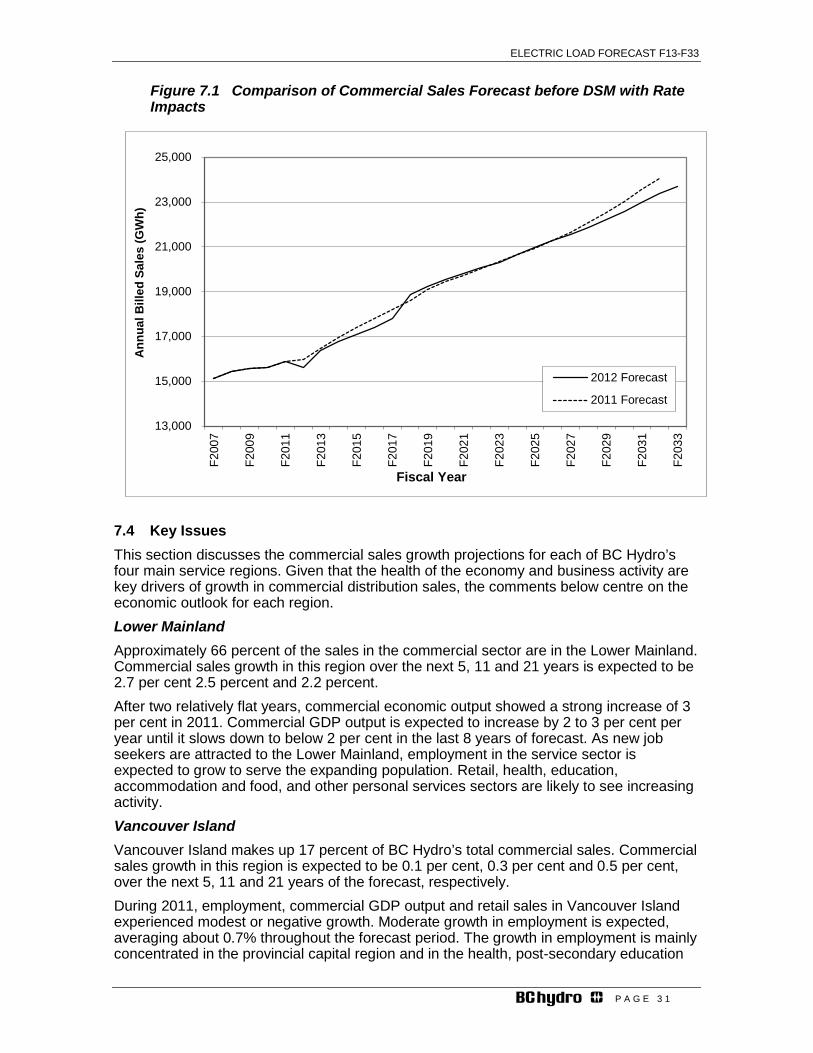
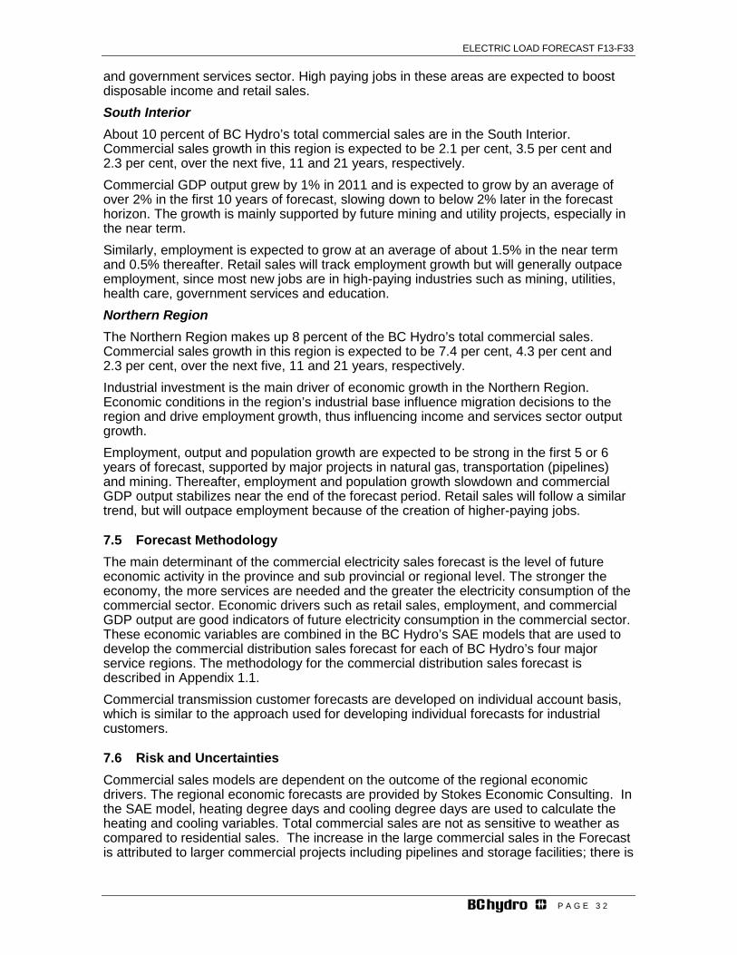
7.2 Forecast Summary Table 7.1 provides a summary of the historical and forecast sales before DSM and with rate impacts6. Electricity consumption in the commercial sector can vary considerably from year to year reflecting the level of activity in the service sector of B.C.’s economy. During F2011, reported billed sales increased by 265 GWh or 1.7 percent, while during F2012 the reported billed sales decreased by 279 GWh or 1.8 percent. The annual average growth rate for commercial sales forecast over the next 5, 11 and 21 years (before DSM with rate impacts) is forecast to be 2.7 per cent, 2.4 per cent and 2.0 per cent, respectively. Commercial distribution, which is the largest portion of total commercial sales, is expected to grow on average by about 300 GWh per annum. Commercial transmission sales are expected to increase in the near term and moderate over the long term; overall commercial transmission sales are expected to grow on average about 80 GWh per annum.
7.3 Commercial Forecast Comparison Figure 7.1 shows the 2012 Forecast of total commercial sales before DSM with rate impacts. Compared to the 2011 Forecast, the current total commercial sales forecast is lower by 73 GWh (-0.4%) in F2013, 381 GWh (-2.1%) in F2017, 29 GWh (-0.1%) in F2023 and 695 GWh (-2.9%) in F2032.
The overall commercial distribution load has been revised downwards which is primarily due to lower projections of economic drivers. Slower economic growth projections for the U.S. and global economies impact tourism and retail spending in BC. Sales to the larger commercial customers such as ports and pipelines are projected to grow significantly over the first five years of the forecast; after these expansions are completed, sales are then expected to remain relatively flat. The forecast for oil and gas loads (i.e., pipelines) are further discussed in Appendix 3.1.
6 Commercial general distribution sales as shown in Table 7.1 include the impact of EV and double counting adjustments for codes and standards.
ELECTRIC LOAD FORECAST F13-F33
P A G E 3 1
Figure 7.1 Comparison of Commercial Sales Forecast before DSM with Rate Impacts
7.4 Key Issues This section discusses the commercial sales growth projections for each of BC Hydro’s four main service regions. Given that the health of the economy and business activity are key drivers of growth in commercial distribution sales, the comments below centre on the economic outlook for each region. Lower Mainland Approximately 66 percent of the sales in the commercial sector are in the Lower Mainland. Commercial sales growth in this region over the next 5, 11 and 21 years is expected to be 2.7 per cent 2.5 percent and 2.2 percent. After two relatively flat years, commercial economic output showed a strong increase of 3 per cent in 2011. Commercial GDP output is expected to increase by 2 to 3 per cent per year until it slows down to below 2 per cent in the last 8 years of forecast. As new job seekers are attracted to the Lower Mainland, employment in the service sector is expected to grow to serve the expanding population. Retail, health, education, accommodation and food, and other personal services sectors are likely to see increasing activity. Vancouver Island Vancouver Island makes up 17 percent of BC Hydro’s total commercial sales. Commercial sales growth in this region is expected to be 0.1 per cent, 0.3 per cent and 0.5 per cent, over the next 5, 11 and 21 years of the forecast, respectively. During 2011, employment, commercial GDP output and retail sales in Vancouver Island experienced modest or negative growth. Moderate growth in employment is expected, averaging about 0.7% throughout the forecast period. The growth in employment is mainly concentrated in the provincial capital region and in the health, post-secondary education
13,000
15,000
17,000
19,000
21,000
23,000
25,000
F200
7
F200
9
F201
1
F201
3
F201
5
F201
7
F201
9
F202
1
F202
3
F202
5
F202
7
F202
9
F203
1
F203
3
Ann
ual B
illed
Sal
es (G
Wh)
Fiscal Year
2012 Forecast
2011 Forecast
ELECTRIC LOAD FORECAST F13-F33
P A G E 3 2
and government services sector. High paying jobs in these areas are expected to boost disposable income and retail sales. South Interior About 10 percent of BC Hydro’s total commercial sales are in the South Interior. Commercial sales growth in this region is expected to be 2.1 per cent, 3.5 per cent and 2.3 per cent, over the next five, 11 and 21 years, respectively. Commercial GDP output grew by 1% in 2011 and is expected to grow by an average of over 2% in the first 10 years of forecast, slowing down to below 2% later in the forecast horizon. The growth is mainly supported by future mining and utility projects, especially in the near term. Similarly, employment is expected to grow at an average of about 1.5% in the near term and 0.5% thereafter. Retail sales will track employment growth but will generally outpace employment, since most new jobs are in high-paying industries such as mining, utilities, health care, government services and education. Northern Region The Northern Region makes up 8 percent of the BC Hydro’s total commercial sales. Commercial sales growth in this region is expected to be 7.4 per cent, 4.3 per cent and 2.3 per cent, over the next five, 11 and 21 years, respectively. Industrial investment is the main driver of economic growth in the Northern Region. Economic conditions in the region’s industrial base influence migration decisions to the region and drive employment growth, thus influencing income and services sector output growth. Employment, output and population growth are expected to be strong in the first 5 or 6 years of forecast, supported by major projects in natural gas, transportation (pipelines) and mining. Thereafter, employment and population growth slowdown and commercial GDP output stabilizes near the end of the forecast period. Retail sales will follow a similar trend, but will outpace employment because of the creation of higher-paying jobs.
7.5 Forecast Methodology The main determinant of the commercial electricity sales forecast is the level of future economic activity in the province and sub provincial or regional level. The stronger the economy, the more services are needed and the greater the electricity consumption of the commercial sector. Economic drivers such as retail sales, employment, and commercial GDP output are good indicators of future electricity consumption in the commercial sector. These economic variables are combined in the BC Hydro’s SAE models that are used to develop the commercial distribution sales forecast for each of BC Hydro’s four major service regions. The methodology for the commercial distribution sales forecast is described in Appendix 1.1. Commercial transmission customer forecasts are developed on individual account basis, which is similar to the approach used for developing individual forecasts for industrial customers.
7.6 Risk and Uncertainties Commercial sales models are dependent on the outcome of the regional economic drivers. The regional economic forecasts are provided by Stokes Economic Consulting. In the SAE model, heating degree days and cooling degree days are used to calculate the heating and cooling variables. Total commercial sales are not as sensitive to weather as compared to residential sales. The increase in the large commercial sales in the Forecast is attributed to larger commercial projects including pipelines and storage facilities; there is

ELECTRIC LOAD FORECAST F13-F33
P A G E 3 3
some uncertainty regarding the completion of large individual projects and their need for electrical service. Factors Leading to Lower than Forecast Commercial Sales:
• A change in the economic conditions as commercial sales tends to follow the major indicators of the economy;
• The pine beetle infestation will cause forestry employment to decline in the long term; this may impact local commercial activity and growth
• Improved equipment efficiency across the end uses; and • The aging provincial population will suppress future employment growth.
Factors Leading to Higher than Forecast Commercial Sales: • A robust economic recovery and increased tourism activity that would create
additional demands for commercial services; • Low interest rates encourage consumer spending; and
• Substantially warmer summers (increasing air conditioning loads) or colder winters (increasing heating loads) relative to historical patterns.
ELECTRIC LOAD FORECAST F13-F33
P A G E 3 4
Table 7.1 Commercial Sales before DSM with Rate Impacts
Fiscal Year
Commercial Sales (GWh) Irrigation,
Street Lights and
BC Hydro Own Use
Commercial General
Distribution Commercial
Transmission Total
Commercial Sales1
Actual F2007 380 13,991 734 15,105 F2008 379 14,230 831 15,439 F2009 368 14,398 811 15,577 F2010 371 14,235 1,025 15,631 F2011 359 14,475 1,062 15,896 F2012 346 14,283 988 15,617
Forecast F2013 366 14,909 1,112 16,387 F2014 368 15,106 1,278 16,752 F2015 370 15,208 1,493 17,071 F2016 371 15,436 1,577 17,384 F2017 372 15,736 1,707 17,815 F2018 374 16,103 2,382 18,859 F2019 376 16,417 2,423 19,216 F2020 379 16,718 2,454 19,551 F2021 382 16,954 2,468 19,804 F2022 384 17,197 2,483 20,064 F2023 387 17,436 2,500 20,323 F2024 389 17,722 2,549 20,660 F2025 391 17,993 2,564 20,948 F2026 394 18,280 2,587 21,260 F2027 396 18,542 2,598 21,536 F2028 399 18,856 2,611 21,865 F2029 401 19,176 2,625 22,202 F2030 403 19,535 2,639 22,577 F2031 406 19,909 2,653 22,968 F2032 408 20,298 2,667 23,374 F2033 411 20,616 2,673 23,700
Growth Rates 5 years*: F2007 to F2012
-1.9% 0.4% 6.1% 0.7%
5 years: F2012 to F2017
1.5% 2.0% 11.6% 2.7%
11 years: F2012 to F2023
1.0% 1.8% 8.8% 2.4%
21 years: F2012 to F2033
0.8% 1.8% 4.9% 2.0%
* Historical growth rates are not weather normalized. Forecast is prepared based on normal weather.
1. Total commercial sales are the sum of Irrigation, Street Lights and BC Hydro Own Use plus Commercial Distribution and Commercial Transmission.

ELECTRIC LOAD FORECAST F13-F33
P A G E 3 5
8 Industrial Forecast
8.1 Sector Description The industrial sector currently comprises about 32 percent of BC Hydro’s total annual sales. It is organized into four main sub-sectors: forestry, mining, oil and gas and other. Industrial customers are involved in extracting, processing and manufacturing resource based commodities which are largely destined for exports. The industrial sector is also organized by voltage service (transmission vs. distribution). Approximately 80% of the total industrial sales are served at transmission voltages (above 60 kV) with the remaining 20% served at distribution voltages (below 60 kV). New LNG facilities, which are categorized as industrial sector load, potentially represent the biggest additional loads on BC Hydro’s system. BC Hydro continues to monitor the development of several potential LNG projects, which are treated as separate scenarios in BC Hydro’s long-term planning processes. More information on potential new LNG demands can be found in Appendix 3.3.
8.2 Forecast Summary Total industrial sales forecast before DSM and rate impacts are shown in Table 8.1 and Table 8.2. Table 8.1 shows a consolidated projection of industrial sales broken down by industry sub-sectors. Table 8.2 shows total industrial sales broken down between transmission and distribution voltage customers. Over the past five years, total industrial sales declined by about 16 percent. This was primarily due to a decline in forestry sales due to structural changes and permanent closures of pulp and paper mills. Total industrial sales in F2013 are expected to increase by 151 GWh or 0.9 percent relative to F2012, with growth in most of the sub-sectors. The five, 11 and 21-year year growth projection of total industrial sales, before DSM and rate impacts is 3.3 percent, 2.5 percent and 1.3 percent, respectively. Looking forward, BC’s industrial customers are expected to have a strong global position due to the quality of the resource base, the demand for B.C.’s natural resources and advanced infrastructure to supply industrial products to market.
8.3 Industrial Forecast Comparison Figure 8.1 compares the 2012 Forecast to the 2011 Forecast (before DSM and rate impacts).
ELECTRIC LOAD FORECAST F13-F33
P A G E 3 6
Figure 8.1 Comparison of Industrial Sales Forecast before DSM and Rate Impacts
8.4 Key Issues and Sector Outlook The following sections describe the outlook, drivers and risk factors for the major industrial sub-sectors. Unless otherwise stated, the comparison between the 2011 Forecast and the 2012 Forecast is based on sales by transmission class customers only.
8.4.1 Forestry The forestry sector accounts for about 60 percent of industrial sales. Forestry is categorized into three sub-sectors: pulp and paper, wood products and chemicals. Although generalizations can be made across the forestry sector (for instance, the impact of the pine beetle infestation and the recent recession), each sub-sector has different sales history, drivers and market characteristics. Forestry sales have changed significantly over the past number of years. It is expected that the demand for forestry sector goods will continue to recover from the 2008-2009 recession. During the past four years, forestry sales declined by about 20 percent, largely due to the pulp and paper and wood product sub-sectors which both experienced shutdowns. In F2013, forestry sales are forecast to decrease by three percent relative to F2012. For the five years ending in F2017, projected sales steadily decline. The decline is attributable to further restructuring measures in the pulp and paper sub-sector and increasing constraints in the wood products sub-sector due to the continuing impact of the pine beetle Infestation. During the F2017-F2022 period, forestry sales remain relatively unchanged with moderate growth in pulp and paper sales being offset by anticipated declines in wood products sales. For the latter 10 years of the forecast period, forestry sales are relatively unchanged from sales in F2023. For details, please see the Overview section below. Pulp and paper sales are forecast to be relatively flat. However, wood products sales remain unchanged as the pine beetle infestation continues to hamper production levels.
-
5,000
10,000
15,000
20,000
25,000
F200
8F2
009
F201
0F2
011
F201
2F2
013
F201
4F2
015
F201
6F2
017
F201
8F2
019
F202
0F2
021
F202
2F2
023
F202
4F2
025
F202
6F2
027
F202
8F2
029
F203
0F2
031
F203
2F2
033
Annu
al B
illed
Sal
es (G
Wh)
Fiscal Year
2012 Forecast
2011 Forecast

ELECTRIC LOAD FORECAST F13-F33
P A G E 3 7
Compared with the 2011 Forecast, the 2012 Forecast is approximately 1,300 GWh lower at the end of the forecast period. This is primarily due to the pulp and paper sub-sector where production expectations for certain product grades have been reduced relative to the 2011 Forecast.
8.4.1.1 Pulp and Paper Overview Transmission pulp and paper sales represent 61 percent of forestry sector sales and 37 percent of industrial sales. Pulp and paper sales are concentrated in 19 mills located primarily in the south-western and north-eastern parts of B.C. These mills produce and export a wide variety of products including newsprint, coated and uncoated groundwood paper, unbleached kraft (UBK) pulp, bleached chemical pulp, thermo-mechanical pulp (TMP) and marked bleached thermo-mechanical pulp (CTMP). Softwood is predominantly used by mills in the Prince George, Quesnel, South Interior and Vancouver Island regions. Hardwood is used by northern mills located in the Chetwynd area. Vancouver Island uses softwood to produce TMP and CTMP. The main drivers for this sub-sector are pulp and paper market prices, the U.S. economy and increasingly, the global economy. Pulp and Paper Outlook Over the past five years, transmission pulp and paper sales declined by about 30 percent largely due to pulp and paper mill and line closures. The factors contributing this large decrease include: aging equipment, declining fibre availability (due to pine beetle infestation), rising prices of recycled feedstock (due to Chinese demand), strong competition from mills in South America, displacement of newspaper by digital media and increased targeting of electronic media by advertisers. In F2013, sales are forecast to decline over the prior year as global economic condition and pulp and paper demand soften. For the first 10 years of the 2012 Forecast, pulp and paper sales are projected to decline by approximately 1,000 GWh or 17 percent. Further mill and line closures are expected to occur as the industry continues to restructure in order to become more competitive. In the latter half of the forecast period, sales are projected to remain flat. During this period, further mill and line closures are expected but there will also be mill and line expansions into areas that better leverage the operational and fibre environment in which B.C. pulp and paper mills operate. Compared to the 2011 Forecast, the 2012 Forecast for pulp and paper is lower by roughly 600 GWh in the first 10 years and lower by over 1,300 GWh in F2032. These reductions are primary the result of lowered production expectations for certain product grades.
Pulp and Paper Drivers and Risk Drivers: • North American paper demand for advertising; • Growing demand for paper products and market pulp by China and other developing
economies because of increased needs for packaging materials and tighter markets for fibre (positive factors for B.C.);
• Global demand for B.C.’s attractive wood fibre which adds strength to recycled papers and a growing number of other applications and products;
• Growing demand for B.C.’s environmentally-friendly pulp and paper (i.e. produced with renewable fuel);

ELECTRIC LOAD FORECAST F13-F33
P A G E 3 8
• Ability of B.C. mills to transition away from kraft pulp and newsprint to higher value products;
• Incentive programs for increased electricity self-generation at kraft mills; and • B.C. having one of the lowest industrial electricity costs in the world. Risk Factors: • Economic swings in the U.S.; • Fibre shortage due to pine beetle infestation. This will reduce fibre supply for B.C. pulp
mills which use residual chips from lumber and whole log chipping; • Competition for fibre supply from bio-fuel and pellet operations; • Ongoing decline in the North American newsprint market, where both shipments and
advertising expenditures have been progressively declining over the last 10 years; • Displacement of B.C. softwood with hardwood pulp by low-cost competitive mills which
continue to be built in the Southern Hemisphere; • Risk of major equipment failure as some assets near end-of-life, with some mills being
forced to close due to a lack of cash flow to fix or replace such capital-intensive assets; • Long-term Chinese demand for pulp and paper; and • Long-term global demand for tissue.
8.4.1.2 Wood Products Overview Wood products represent about 23 percent of forestry sector sales. BC Hydro provides electricity to more than 100 wood products mills located in every major region of B.C., particularly the North Coast, Central Interior and Southern Interior which contain 75 percent of the mills. These facilities produce dimensional and structural lumber, oriented strand board (OSB), medium density fiberboard, plywood, fuel pellets and other specialty products.
The primary drivers for wood products demand are housing starts and repair and remodeling. B.C.’s share of the U.S. lumber market is greater than all other non-U.S. producers combined. Furthermore, B.C. could soon displace Russia as the dominant lumber supplier to the Chinese market.
The B.C. Interior has some of the lowest cost producers of lumber in the world. However, sawmill and plywood plant production will be constrained by saw-log availability due to the mountain pipe beetle (MPB) devastation in the forests of B.C. Although the Ministry of Forests is undertaking measures to address the impact, it is anticipated that forest management practices will be imposed (i.e., limiting the annual allowable cut) such that lumber production will be dramatically reduced. A sustainable level of logging and annual allowable cut is expected to be reached around 2024. Thereafter, wood products sales are expected to remain flat for the duration of the forecast period.
Wood Products Outlook The 2008-09 recessions had a devastating effect on the wood products sub-sector. Over the last five years, sales fell by 21 percent due primarily to depressed U.S. housing starts. In F2013, wood products sales are forecast to increase modestly due to growth in U.S. housing starts and lumber exports to China. In the near term, sales are expected to increase moderately due to growing demand from China, a recovery in U.S. housing starts and construction activity in post-tsunami Japan. For the five year period starting in F2017, B.C. wood products sales are expected to
ELECTRIC LOAD FORECAST F13-F33
P A G E 3 9
progressively decline. As demand for B.C. wood products will exceed the industry’s ability to supply due to constraints caused by the Mountain Pine Beetle. For beetle-killed trees, the amount of useable lumber diminishes over time due to deterioration. Over the last 10 years of the forecast period, wood product sales are projected to remain flat, although below historical levels, and below market demand. BC Hydro expects B.C. forest management practices to successfully achieve a sustainable annual cut level which in turn will stabilize lumber production.
Compared to the 2011 Forecast, the 2012 Forecast for wood products is lower in the short to medium term (demand weakness and a more constraining effect of the MPB impact on useable log availability) and slightly higher in the long term due to assumptions with respect to the severity of the pine beetle infestation on the wood products sub-sector.
Wood Products Drivers and Risk Drivers: • U.S. housing starts (currently are less than one half/the level required to match U.S.
population growth); • Repair and remodeling demand in the U.S., • Chinese demand for roof trusses and framing for houses and small apartments; • Japanese housing starts (demand for hemlock and SPF); and • Demand from other areas in the world such as Korea, India, Taiwan, Hong Kong,
Singapore and the Middle East. Risk Factors: • The effect of the U.S. economy on the recovery of U.S. housing starts; • A softwood lumber trade issues with the U.S.; • Harvest life of trees killed by the Mountain Pine Beetle; • Medium to long run severity of pine beetle infestation; • Higher harvesting costs for B.C. coastal sawmills (caused by steep terrain, outdated
equipment and relatively high labour costs); • Ability of industry in B.C. Interior to transition towards processing higher volumes of
beetle-killed timber; and • Ability of B.C.-based OSB producers to continue to improve products for markets.
8.4.1.3 Chemicals Overview Chemicals represent about 16 percent of forestry sector sales. Sales are primarily to customers who produce bleaching agents for the pulp and paper industry, for customers who produce cleaning agents for the oil and gas industry and for water purification. Chemical sales are strongly correlated to the health of the pulp and paper industry, particularly the global industry given that much of the product is destined for export. Since chemical companies use electrolysis to producer their bleaching agents, electricity forms a large part of their operating costs.
Chemicals Outlook Over the past four years, sales in this sector have remained relatively flat with modest dips that arose due to closures of pulp and paper mills and lines in B.C. In F2011, sales were particularly low due to an extended downtime at a large customer facility experiencing a

ELECTRIC LOAD FORECAST F13-F33
P A G E 4 0
complete plant makeover. In F2013, sales are forecast to decrease slightly from the previous year as plant operational improvements were recently made at a couple of facilities thereby decreasing electricity requirements per unit of output. In the near term, chemical sales are expected to slowly increase as some facilities are expanded to meet growing demand for bleaching and cleaning agents, some of which is driven by exports. In the medium and long term, sales are projected to only modestly grow due to weak demand in the B.C. pulp and paper sector, but otherwise stimulated by growing demand for cleaning agents (for the oil and gas industry) and water purification agents (for municipalities). Much of this demand growth in the latter half of the forecast period will be export-based.
Chemical Drivers and Risk Drivers: • Pulp and paper demand; • Global economy; and • Oil and gas activity. Risk Factors: • Electricity rate increases; • Closure of B.C. pulp mills; and • Capability of some chemical customers to transition into producing the type of
bleaching agents that can be exported outside of B.C. 8.4.1.4 Forestry Methodology The 2012 Forecast for the forestry sector was developed by initially assessing last year’s forecast. BC Hydro determined that updated information was required for several areas including: (i) a forecast of lumber exports to China (ii) the expected impact of the pine beetle infestation; and (iii) customer mill production. To obtain the necessary information, BC Hydro retained consultants with relevant forestry expertise. The consulting team produced mill production forecasts for all B.C. mills and for various product lines, using several inputs, including long term GDP forecast for countries that purchase B.C. forestry products. BC Hydro incorporated these production forecasts into its load forecasting model to create a sector forecast. The forestry forecast also considered issues such as customers with onsite generation, electricity purchase agreements, historical consumption and electricity consumption intensities, as well as input from BC Hydro’s Key Account Managers. BC Hydro developed the forestry sector forecast by multiplying facility production forecasts by the electricity intensity forecast.
8.4.2 Mining The mining sector accounts for about 17 percent of total industrial sales. It is categorized into two sub-sectors: metal and coal mines. Metal mining makes up for 78% of the current mining sector load. For mining customers, electricity is mostly used for ore extraction, crushing and processing. In the short run, mining sales are not highly sensitive to economic drivers and mineral price movements since existing mines tend to produce continuously through commodity price cycles. In the medium to long term, mining expansions (or attritions), start-ups (or closures) and new project advancements (or deferrals) are sensitive to economic conditions and mineral prices.
ELECTRIC LOAD FORECAST F13-F33
P A G E 4 1
The Asia-Pacific region is important for the health of mining in B.C. because more than two-thirds of mining exports are shipped to Japan, China and South Korea. The future outlook for mining is also shaped by mineral exploration, which in turn is influenced by provincial policy. Exploration expenditures in BC increased to record highs following the recession of 2008-2009 to meet the surging demand for metal from Chinese and Indian markets. The mining sector invested an estimated $680 million in exploration in 2012, a 47% increase over the previous year’s $462 million which was a record year for exploration in British Columbia. Nonetheless, due to a recent slowdown in growth in China’s economy, recession in the EU and Japan and prolonged recovery process in other developed countries such as the US, the rate of acquisition and foreign investment in the mining sector has cooled off in 2012, after intense activity between 2009 and 2011. Part of the explanation is that mining companies are starting to feel the pressure of higher costs and tighter budgets. 2012 represented a challenging year for the mining sector. On the positive side, New Afton mine was brought into production last summer; Thompson Creek has successfully completed the expansion project at Endako mine replacing the old mill in March 2012. In addition, construction is well underway at Mount Milligan mine with expected start-up in mid-2013, while construction work at Red Chris mine has begun. Expansion projects are continuing on schedule at Gibraltar Mine and Highland Valley Copper while Mount Polley has publically announced the extension of mining operations to 2022. Nonetheless, access to financing has become an issue for smaller companies, while lower commodity outlooks for molybdenum, copper or coal have affected most of the competitors. Faced with continued depressed prices for molybdenum as well as operational problems, Thompson Creek has decided to temporarily shut down mining operations at Endako in July 2012. While the newly commissioned $500 million mill would still operate on stockpiles, the low molybdenum prices may continue to hamper profitability. Additionally, cost outruns at Mt Milligan have forced Thompson Creek to sell rights to future gold production and implement cost saving measures at other mining operations in order to raise necessary financing to complete the project. Teck has also announced in the fall of 2012 that the $1.5-billion of planned spending in 2012 and 2013 is being pushed out to the future. The company is facing permitting delays at the Quintette coal mine project in Northeast BC. Disputes over the employment of foreign workers in coal mining operations in Northeast BC as well as First Nation opposition to a series of projects (most notably New Prosperity) could delay or cancel the development of several new mines. In spite of the recent pressure on the mining sector, the 2012 Mining Forecast load still grows significantly in the next few years of the forecast. Most of the growth is, however, the result of new projects recently energized and expected to wrap up or expansions to existing operations. The 2012 Mining Forecast is lower compared to the 2011 Forecast due to increased uncertainty in the economic outlook and lower commodity price outlooks. Short term surplus and depressed prices continue to be a concern for molybdenum operations, while a slowdown in steelmaking activity has cooled off the metallurgical coal markets after several years of steady increases, driven by construction activity in Asia. The forecast is also lower as a result of a recent decision of the Provincial government to reject Morrison mine environmental permit. While the current environment has negatively affected some metal mine projects, the increased economic uncertainty has maintained the interest in gold operations. Additionally, existing copper-gold mines that are not facing large investment decisions are still fairly well positioned to increase production and push back shutdown dates.

ELECTRIC LOAD FORECAST F13-F33
P A G E 4 2
Despite a recent slowdown in growth, China is still expected to fuel long-term activity in the BC mining sector.
8.4.2.1 Metal Mines Overview
Metal Mines Outlook BC metal mining sector includes copper, gold, silver, molybdenum, lead and zinc operations. In the long term, electricity sales to mines are tied to price expectations for copper, molybdenum and gold. The prices of these commodities are influenced by global demand and supply and the state of the global economies. In the short term on a month to month basis, electricity sales to metal mines are relatively independent of commodity price fluctuations because these mines are predominantly fixed-cost operations which typically need to run continuously. Mining sales are not overly dependent on domestic economic activity but are more correlated to the global economy since the most of BC metal mining production is exported. The top destinations for BC metallic mineral exports include Japan, the United States, China and Korea. Since early 2009, the metal mining sector in B.C. has benefited from strong copper and gold prices. British Columbia is viewed as an attractive environment for global mining investment. Sales to metal mining customers in short term are expected to increase due to start-up or ramp ups of several newly commissioned mines as well as expansions to existing facilities. In the medium to long term, metal mine sales are expected to peak at approximately 5,000 GWh per year around 2020 as new mines come online and several existing mines ramp up production. The long term demand for copper and molybdenum is expected to be driven by high demand from Asia and to some extent recovering Western economies. The forecast decreases to 4,000 GWh per year long term as some of the large operations shut down. Compared to the 2011 Forecast, this year’s metal mining sales forecast is significantly lower overall as several new projects have deferred start dates. Probabilities to several new mines have been lowered due to increased uncertainty in the economic and commodity outlook.
Metal Mine Drivers and Risk Drivers:
• Copper, gold and molybdenum prices which in turn are driven by economic activity • Industry perception of the resource friendliness of the B.C. government and its
present and future tax regime; and • Level of supporting infrastructure (ports, roads, power and proximity to
communities) and the potential for future development. Risk Factors:
• Future provincial and federal government actions that increase or decrease clarity of Regulatory policy, conflict resolution measures, and tax efficiencies;
• Outcome of future Environmental Assessment applications, particularly with regard to First Nations issues; and
• Aging workforce and the looming wave of retirements over the next years. According to a report released in 2012 by the Mining Industry Human Resources Council in partnership with the BC Mining HR Task Force, British Columbia will employ over 16,700 mining professionals in the next 10 years. However the study

ELECTRIC LOAD FORECAST F13-F33
P A G E 4 3
acknowledges that human resources challenges continue to threaten the future competitiveness of the BC mining industry.
8.4.2.2 Coal Mines Overview Coal mines comprise about 22% percent of BC Hydro’s mining sector sales. The coal is predominantly produced in southeastern B.C. with the larger coal mining customers in this region accounting for roughly 90 percent of total sales. Coal is also produced in the northeastern B.C., which currently has a small production share but is expected to grow significantly. The single mine on Vancouver Island produces thermal coal. Elk Valley Coal Partnership, which owns five mines in southeastern B.C., is the second biggest supplier of metallurgical coal in the world. Metallurgical coal is an export commodity which is sold worldwide to integrated steel mills for steel-making purposes. In the long term, coal mining sales are tied to price expectations for coal, which is largely driven by metallurgical coal demand. Markets for British Columbia coal include Japan, China, South Korea and India, Europe, South America and the US but shipments to Asian countries represent more than 50% of BC coal exports. As a result, the state of the BC economy has little effect on coal sales but provincial regulatory and policy actions can have a significant impact. Most of the coal produced in southeast BC is transported by rail to the Westshore Terminals; coal produced by the northeast BC mines is shipped via Ridley Terminals Inc.’s in Prince Rupert while the coal produced on Vancouver Island is exported via Texada Island and Neptune Terminals in Vancouver. The aforementioned terminals were or will be subject to significant upgrades in the coming years to accommodate the higher volume of coal shipments and cargo traffic. The provincial and federal governments recently pledged $750 million "that will improve rail efficiency and add capacity for coal and other export bulk commodities.”7
Coal Mines Outlook The price for metallurgical coal has weakened recently after a strong five-year run spurred by rising demand from Asia, and particularly China. Additionally, global uncertainty has forced several companies to revise capital expenditures in short term. In the 2012 Forecast, short-term coal mining sales are expected to stay relatively flat in the next couple of years and increase past F2014 with the anticipated start-up of new mines. Over the long term, the distribution and transmission coal sales growth is projected to slow due to more moderate expectations of growth in the global economy, rail line and mine constraints in BC. Compared to the 2011 Forecast, the current forecast is lower in short, medium and long term. This is largely the result of decreased expectations for several new coal mine projects as a result of lower global economic outlook and deferred capital expenditure.
Nonetheless, the coal forecast is still increasing by more than 30% by F2017 relative to F2012 sales, sustained by global demand for metallurgical coal, particularly from China and India.
Coal Mine Drivers and Risk Drivers:
7 http://www2.news.gov.bc.ca/news_releases_2009-2013/2010TRAN0104-001386.htm

ELECTRIC LOAD FORECAST F13-F33
P A G E 4 4
• Demand for steel in Japan, South Korea, China, the European Union and India; and
• Global economic outlook, particularly in Asia and the U.S. • Increased coal export capacity
Risk Factors: • Expanded Australian coal production. Australia accounts for roughly two-thirds of
the • global metallurgical coal production; • First Nation opposition and increasing environmental and local opposition • Disputes over the employment of foreign workers in coal mining operations have
the potential to delay projects such as Murray River or Gething • B.C. mining construction costs; • Rail and terminal capacity constraints; and • Future policies or regulations that could impact coal exploration or development.
8.4.2.3 Mining Methodology To develop the 2012 Forecast for coal mining, BC Hydro relied upon a consulting team with a proven record that annually publishes a BC mining report which includes production forecasts and metrics. In addition to the consultant’s report, BC Hydro used several other internal sources (BC Hydro Key Account Managers, Marketing, Powersmart, intelligence from BC Hydro’s Interconnection Group), external sources (company reports, industry reports) as well as its own judgement to assign risk probability weightings to new mines and expansion projections. As such, the forecast is developed on an in depth analysis that involves intensity, production and probability assessments or risk factors.
8.4.2 Oil and Gas Oil and gas loads exist in both the industrial and commercial sectors. The forecast outlook and drivers for the oil and gas sector are fully described in Appendix 3.1. In addition, Appendix 3.2 provides an overview of the unconventional shale gas sub-sector in northeastern B.C.
8.4.3. Other Industrials In F2012, sales to Industrial Other category, as shown in Table 8.2, makes up 2.1 per cent of total industrial sales.
8.4.3.1. Other Industrials Overview
A sizable portion of the transmission customers includes cement companies and auto parts manufacturers. Accordingly, sales are relatively sensitive the provincial economy.
8.4.3.2. Other Industrials Outlook As shown in Table 8.2, sales in F2013 are expected to rise by 8.7 per cent over the previous year. Cement sales are expected to remain relatively strong driven by a rebound in construction activity in North America and continuing growth in Asia. In long run, sales growth slows down to roughly 0.7 per cent per year as it is expected that the provincial and global economic growth rate slows down.

ELECTRIC LOAD FORECAST F13-F33
P A G E 4 5
Compared with the 2011 Forecast, the 2012 Forecast is generally slightly below the 2011 Forecast. This reflects updated information on the expansion plans for several customers as well as a marginally lower long term economic growth.
Other Sector Drivers and Risk: Drivers
• Provincial economic growth. • Construction activity, which in turn affects the demand for cement companies.
Risk factors:
• Economic slowdown or sectorial shifts in BC economy • Increased environmental regulations may affect competitiveness of large cement
producers.
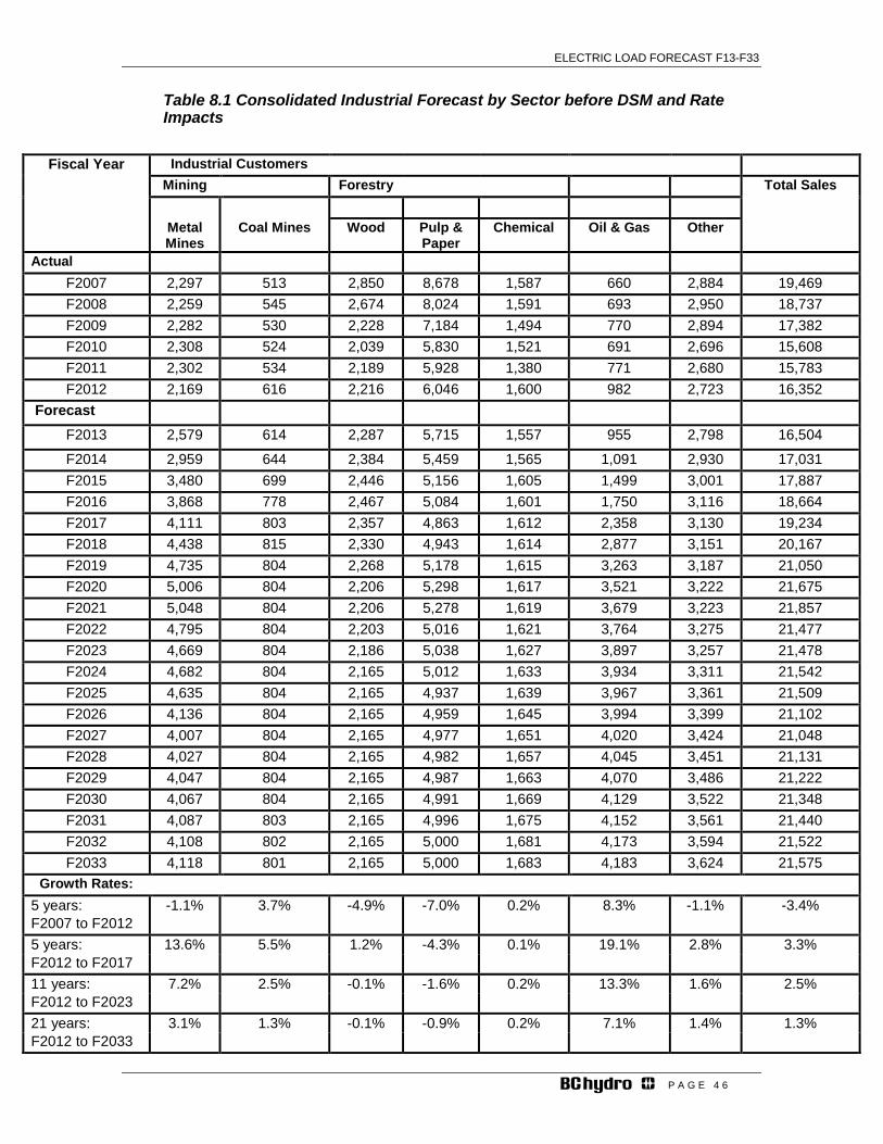
ELECTRIC LOAD FORECAST F13-F33
P A G E 4 6
Table 8.1 Consolidated Industrial Forecast by Sector before DSM and Rate Impacts
Fiscal Year Industrial Customers Mining Forestry Total Sales Metal
Mines Coal Mines Wood Pulp &
Paper Chemical Oil & Gas Other
Actual F2007 2,297 513 2,850 8,678 1,587 660 2,884 19,469 F2008 2,259 545 2,674 8,024 1,591 693 2,950 18,737 F2009 2,282 530 2,228 7,184 1,494 770 2,894 17,382 F2010 2,308 524 2,039 5,830 1,521 691 2,696 15,608 F2011 2,302 534 2,189 5,928 1,380 771 2,680 15,783 F2012 2,169 616 2,216 6,046 1,600 982 2,723 16,352
Forecast
F2013 2,579 614 2,287 5,715 1,557 955 2,798 16,504
F2014 2,959 644 2,384 5,459 1,565 1,091 2,930 17,031 F2015 3,480 699 2,446 5,156 1,605 1,499 3,001 17,887 F2016 3,868 778 2,467 5,084 1,601 1,750 3,116 18,664 F2017 4,111 803 2,357 4,863 1,612 2,358 3,130 19,234 F2018 4,438 815 2,330 4,943 1,614 2,877 3,151 20,167 F2019 4,735 804 2,268 5,178 1,615 3,263 3,187 21,050 F2020 5,006 804 2,206 5,298 1,617 3,521 3,222 21,675 F2021 5,048 804 2,206 5,278 1,619 3,679 3,223 21,857 F2022 4,795 804 2,203 5,016 1,621 3,764 3,275 21,477 F2023 4,669 804 2,186 5,038 1,627 3,897 3,257 21,478 F2024 4,682 804 2,165 5,012 1,633 3,934 3,311 21,542 F2025 4,635 804 2,165 4,937 1,639 3,967 3,361 21,509 F2026 4,136 804 2,165 4,959 1,645 3,994 3,399 21,102 F2027 4,007 804 2,165 4,977 1,651 4,020 3,424 21,048 F2028 4,027 804 2,165 4,982 1,657 4,045 3,451 21,131 F2029 4,047 804 2,165 4,987 1,663 4,070 3,486 21,222 F2030 4,067 804 2,165 4,991 1,669 4,129 3,522 21,348 F2031 4,087 803 2,165 4,996 1,675 4,152 3,561 21,440 F2032 4,108 802 2,165 5,000 1,681 4,173 3,594 21,522 F2033 4,118 801 2,165 5,000 1,683 4,183 3,624 21,575
Growth Rates: 5 years: -1.1% 3.7% -4.9% -7.0% 0.2% 8.3% -1.1% -3.4% F2007 to F2012 5 years: 13.6% 5.5% 1.2% -4.3% 0.1% 19.1% 2.8% 3.3% F2012 to F2017 11 years: 7.2% 2.5% -0.1% -1.6% 0.2% 13.3% 1.6% 2.5% F2012 to F2023 21 years: 3.1% 1.3% -0.1% -0.9% 0.2% 7.1% 1.4% 1.3% F2012 to F2033
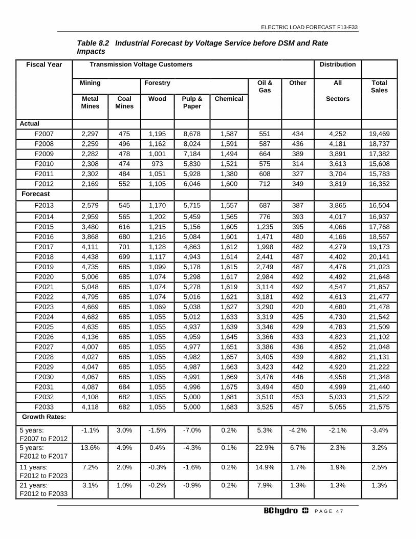
ELECTRIC LOAD FORECAST F13-F33
P A G E 4 7
Table 8.2 Industrial Forecast by Voltage Service before DSM and Rate Impacts
Fiscal Year Transmission Voltage Customers Distribution
Mining Forestry Oil & Gas
Other All Total Sales
Metal Mines
Coal Mines
Wood Pulp & Paper
Chemical Sectors
Actual
F2007 2,297 475 1,195 8,678 1,587 551 434 4,252 19,469 F2008 2,259 496 1,162 8,024 1,591 587 436 4,181 18,737 F2009 2,282 478 1,001 7,184 1,494 664 389 3,891 17,382 F2010 2,308 474 973 5,830 1,521 575 314 3,613 15,608 F2011 2,302 484 1,051 5,928 1,380 608 327 3,704 15,783 F2012 2,169 552 1,105 6,046 1,600 712 349 3,819 16,352
Forecast
F2013 2,579 545 1,170 5,715 1,557 687 387 3,865 16,504
F2014 2,959 565 1,202 5,459 1,565 776 393 4,017 16,937 F2015 3,480 616 1,215 5,156 1,605 1,235 395 4,066 17,768 F2016 3,868 680 1,216 5,084 1,601 1,471 480 4,166 18,567 F2017 4,111 701 1,128 4,863 1,612 1,998 482 4,279 19,173 F2018 4,438 699 1,117 4,943 1,614 2,441 487 4,402 20,141 F2019 4,735 685 1,099 5,178 1,615 2,749 487 4,476 21,023 F2020 5,006 685 1,074 5,298 1,617 2,984 492 4,492 21,648 F2021 5,048 685 1,074 5,278 1,619 3,114 492 4,547 21,857 F2022 4,795 685 1,074 5,016 1,621 3,181 492 4,613 21,477 F2023 4,669 685 1,069 5,038 1,627 3,290 420 4,680 21,478 F2024 4,682 685 1,055 5,012 1,633 3,319 425 4,730 21,542 F2025 4,635 685 1,055 4,937 1,639 3,346 429 4,783 21,509 F2026 4,136 685 1,055 4,959 1,645 3,366 433 4,823 21,102 F2027 4,007 685 1,055 4,977 1,651 3,386 436 4,852 21,048 F2028 4,027 685 1,055 4,982 1,657 3,405 439 4,882 21,131 F2029 4,047 685 1,055 4,987 1,663 3,423 442 4,920 21,222 F2030 4,067 685 1,055 4,991 1,669 3,476 446 4,958 21,348 F2031 4,087 684 1,055 4,996 1,675 3,494 450 4,999 21,440 F2032 4,108 682 1,055 5,000 1,681 3,510 453 5,033 21,522 F2033 4,118 682 1,055 5,000 1,683 3,525 457 5,055 21,575
Growth Rates:
5 years: -1.1% 3.0% -1.5% -7.0% 0.2% 5.3% -4.2% -2.1% -3.4% F2007 to F2012 5 years: 13.6% 4.9% 0.4% -4.3% 0.1% 22.9% 6.7% 2.3% 3.2% F2012 to F2017 11 years: 7.2% 2.0% -0.3% -1.6% 0.2% 14.9% 1.7% 1.9% 2.5% F2012 to F2023 21 years: 3.1% 1.0% -0.2% -0.9% 0.2% 7.9% 1.3% 1.3% 1.3% F2012 to F2033
ELECTRIC LOAD FORECAST F13-F33
P A G E 4 8
9 Non-Integrated Areas and Other Utilities Forecast
9.1. Non Integrated Area Summary
Characteristics – The Non Integrated Areas (NIA) include the Purchase Areas, Zone II and Fort Nelson. Load estimate for Fort Nelson is not included in the Integrated System Load forecast as it is connected to the Alberta transmission grid instead of the BC Hydro grid. A number of small communities located in the Northern and Southern parts of B.C. that are not connected to BC Hydro’s electrical grid make up the Purchase Areas and Zone II. The Purchase Area consists of six locations in the South Interior, namely Lardeau, Crowsnest, Newgate, Kingsgate-Yahk, Kelly Lake, and Keenleyside Dam. To serve customers in the Purchase Area, BC Hydro purchases electricity from a number of neighbouring electric utilities. Zone II consists of ten locations in the Northern Region, namely Masset, Sandspit, Atlin, Dease Lake, Eddontenajon, Telegraph Creek, Anahim Lake, Bella Bella, Bella Coola and Toad River. In F2012, sales to the total NIA represented about 0.5% of total BC Hydro service area sales. In F2012, annual sales in the Purchase Area, Zone II, and Fort Nelson were approximately 13 GWh, 103 GWh, and 167 GWh respectively. Fort Nelson sales accounted for about 60% of all the sales in the NIA. Drivers – For the Purchase Area, the forecast is developed by a trend analysis of the total energy and capacity requirements for each location that makes up the Purchase Area. For Zone II and Fort Nelson, forecasts are developed on a customer sector basis. The drivers for residential sales are housing starts and the average annual use per account. A housing starts forecast is provided by external sources. The average annual use per account in Zone II is based on a statistically adjusted end use (SAE) model. For Zone II, the driver for commercial and industrial sales is the population forecast provided by BC Stats. The driver for small commercial and industrial sales within the Fort Nelson area is the employment forecast provided by consultants. For Fort Nelson, the large industrial accounts at the distribution and transmission level represent a significant part of the load. The forecast for each large industrial customer is developed separately. Increased activity in the oil and gas sector in the Horn River basin, north of the city of Fort Nelson, is anticipated to have an impact on sales within the municipality. As such Fort Nelson sales are expected to have the highest growth rates amongst all NIA communities. Trends and New Developments Table 9.1, 9.2 and 9.3 show the sales, total gross requirements and total peak demand forecast for the Purchase Areas, Zone II and Fort Nelson. Sales within Zone II grew at an average annual rate of 0.4% over the last 5 years and they are expected to grow by 2%, 1.2% and 0.7% annually over the next 5, 11 and 21 years. Total sales within Fort Nelson have declined by 15% since F2009 mainly due to reduced sales to the wood products sector. It is expected that sales will recover and grow relatively steadily into the medium term. This growth will be fuelled by future oil and gas activity which is anticipated to increase sales to residential and commercial customers connected to the Fort Nelson distribution system. In addition, some increase in sales to larger conventional oil and gas customers is expected over the forecast period. Consistent with the 2011 Forecast, sales and peak demand requirements for unconventional gas producers within the Horn River basin are not included in the 2012 load projections for Fort Nelson. BC Hydro has constructed scenarios that examine various Horn River shale gas play load requirements and alternatives on how to supply

ELECTRIC LOAD FORECAST F13-F33
P A G E 4 9
these loads8. Risks and Uncertainties – The main risks to the NIA forecast are discrete events such as the opening or closing of a large new account and developments in Northeast BC, particularly the rate of gas resource development. This is impacted by natural gas prices and the rate of economic growth.
8 These supply scenarios are in BC Hydro planning process.
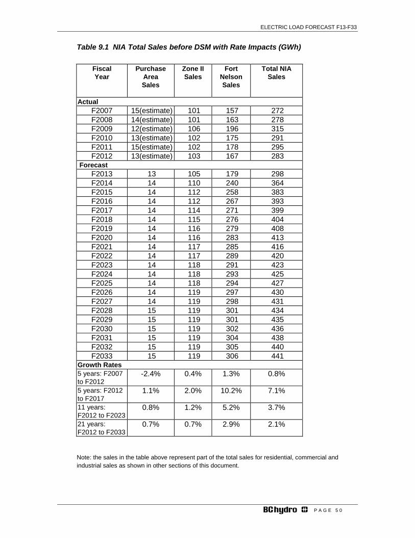
ELECTRIC LOAD FORECAST F13-F33
P A G E 5 0
Table 9.1 NIA Total Sales before DSM with Rate Impacts (GWh)
Fiscal Year
Purchase Area Sales
Zone II Sales
Fort Nelson Sales
Total NIA Sales
Actual F2007 15(estimate) 101 157 272 F2008 14(estimate) 101 163 278 F2009 12(estimate) 106 196 315 F2010 13(estimate) 102 175 291 F2011 15(estimate) 102 178 295 F2012 13(estimate) 103 167 283
Forecast F2013 13 105 179 298 F2014 14 110 240 364 F2015 14 112 258 383 F2016 14 112 267 393 F2017 14 114 271 399 F2018 14 115 276 404 F2019 14 116 279 408 F2020 14 116 283 413 F2021 14 117 285 416 F2022 14 117 289 420 F2023 14 118 291 423 F2024 14 118 293 425 F2025 14 118 294 427 F2026 14 119 297 430 F2027 14 119 298 431 F2028 15 119 301 434 F2029 15 119 301 435 F2030 15 119 302 436 F2031 15 119 304 438 F2032 15 119 305 440 F2033 15 119 306 441
Growth Rates 5 years: F2007 to F2012
-2.4% 0.4% 1.3% 0.8%
5 years: F2012 to F2017
1.1% 2.0% 10.2% 7.1%
11 years: F2012 to F2023
0.8% 1.2% 5.2% 3.7%
21 years: F2012 to F2033
0.7% 0.7% 2.9% 2.1%
Note: the sales in the table above represent part of the total sales for residential, commercial and industrial sales as shown in other sections of this document.
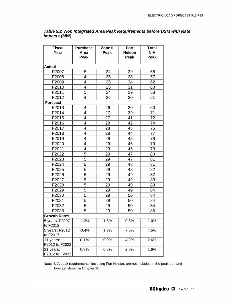
ELECTRIC LOAD FORECAST F13-F33
P A G E 5 1
Table 9.2 Non Integrated Area Peak Requirements before DSM with Rate Impacts (MW)
Fiscal Year
Purchase Area Peak
Zone II Peak
Fort Nelson Peak
Total NIA
Peak
Actual F2007 5 24 29 58 F2008 4 25 28 57 F2009 4 25 34 62 F2010 4 25 31 60 F2011 5 24 29 58 F2012 4 26 30 61
Forecast F2013 4 26 30 60 F2014 4 27 39 71 F2015 4 27 41 72 F2016 4 28 42 74 F2017 4 28 43 76 F2018 4 28 44 77 F2019 4 29 45 78 F2020 4 29 46 79 F2021 4 29 46 79 F2022 5 29 47 80 F2023 5 29 47 81 F2024 5 29 48 81 F2025 5 29 48 82 F2026 5 29 49 82 F2027 5 29 49 83 F2028 5 29 49 83 F2029 5 29 49 84 F2030 5 29 50 84 F2031 5 29 50 84 F2032 5 29 50 84 F2033 5 29 50 85
Growth Rates 5 years: F2007 to F2012
-1.3% 1.6% 0.8% 1.0%
5 years: F2012 to F2017
-0.4% 1.3% 7.5% 4.5%
11 years: F2012 to F2023
0.1% 0.9% 4.2% 2.6%
21 years: F2012 to F2033
0.3% 0.5% 2.5% 1.6%
Note: NIA peak requirements, including Fort Nelson, are not included in the peak demand forecast shown in Chapter 10.

ELECTRIC LOAD FORECAST F13-F33
P A G E 5 2
9.2 Other Utilities & Firm Export The other utilities served by BC Hydro are: City of New Westminster, FortisBC, Seattle City Light and Hyder. The City of New Westminster is surrounded by BC Hydro’s Lower Mainland region. The FortisBC service area is part of southeastern B.C., Seattle City Light is in the state of Washington, and Hyder is in the state of Alaska. Hyder is served at distribution voltage whereas the other three utilities are served at transmission voltage. Pursuant to a BCUC decision dated June 9, 1993, BC Hydro is obligated to provide FortisBC with up to 200 MW of capacity and associated energy under tariff rates. BC Hydro is obligated to serve Seattle City Light in accordance with a treaty between British Columbia and Seattle dated March 30, 1984. The treaty expires on January 1, 2066. The community of Stewart, B.C. is connected to BC Hydro’s grid. Since Hyder, Alaska is only five km away from Stewart, BC Hydro also serves the Alaskan community. In F2012, annual energy sales to City of New Westminster, FortisBC, Seattle City Light, and Hyder were 454 GWh, 514 GWh, 311 GWh, and 1 GWh, respectively.
9.2.1 Forecast Drivers The forecast for the City of New Westminster is based on trend analysis and information from BC Hydro’s distribution planners on new potential larger projects. Previously, BC Hydro’s forecast of sales to FortisBC was based on information received annually from that utility. For the 2012 Forecast, projected sales to FortisBC are additionally based on a comparison of the relative cost of purchasing electricity from BC Hydro (including rate projections) under the 3808 Tariff versus the cost of spot market purchases. The results of this analysis was to decrease the forecasted sales to FortisBC by about 500 GWh per year in the near and middle of the forecast period. Long-term sales forecasts were only slightly modified. The forecast for Seattle City Light is prescribed within the treaty, and the sales forecast for Hyder remains at 1 GWh per year.
9.2.2 Trends and Risks The City of New Westminster is forecast to have modest average annual growth rate of about 1.3 per cent over the entire forecast period. The forecast for sales to FortisBC is lower than last year’s forecast given that market prices have recently been lower than BC Hydro’s 3808 Tariff. Both Seattle City Light and Hyder are forecast to have no significant growth.
The main risk to the forecast for the City of New Westminster is a discrete event such as a large new account. The main risk to the forecast for FortisBC would be a possible change in how that utility plans to meet its supply requirements. Given that the forecast for Seattle City Light is based on a signed treaty, there is minimal sales risk over the entire forecast period. The sales risk for Hyder is also minimal given that its load is so small.
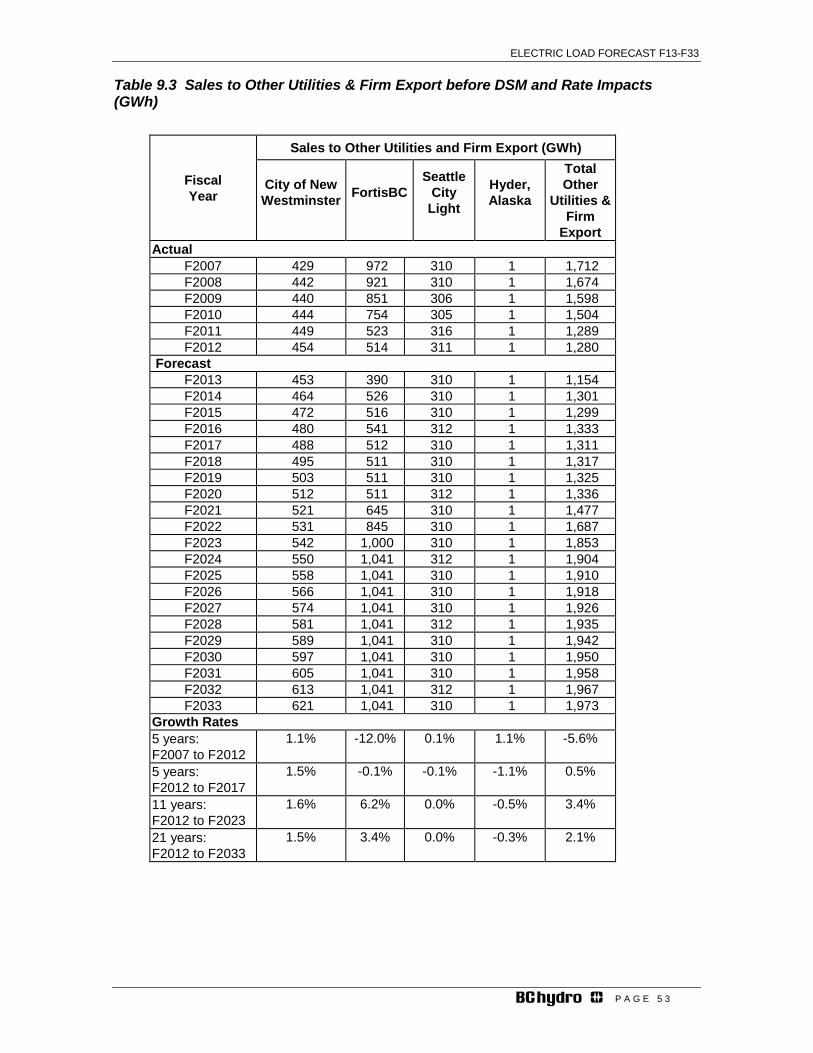
ELECTRIC LOAD FORECAST F13-F33
P A G E 5 3
Table 9.3 Sales to Other Utilities & Firm Export before DSM and Rate Impacts (GWh)
Fiscal Year
Sales to Other Utilities and Firm Export (GWh)
City of New Westminster
FortisBC
Seattle City
Light
Hyder, Alaska
Total Other
Utilities & Firm
Export Actual
F2007 429 972 310 1 1,712 F2008 442 921 310 1 1,674 F2009 440 851 306 1 1,598 F2010 444 754 305 1 1,504 F2011 449 523 316 1 1,289 F2012 454 514 311 1 1,280
Forecast F2013 453 390 310 1 1,154 F2014 464 526 310 1 1,301 F2015 472 516 310 1 1,299 F2016 480 541 312 1 1,333 F2017 488 512 310 1 1,311 F2018 495 511 310 1 1,317 F2019 503 511 310 1 1,325 F2020 512 511 312 1 1,336 F2021 521 645 310 1 1,477 F2022 531 845 310 1 1,687 F2023 542 1,000 310 1 1,853 F2024 550 1,041 312 1 1,904 F2025 558 1,041 310 1 1,910 F2026 566 1,041 310 1 1,918 F2027 574 1,041 310 1 1,926 F2028 581 1,041 312 1 1,935 F2029 589 1,041 310 1 1,942 F2030 597 1,041 310 1 1,950 F2031 605 1,041 310 1 1,958 F2032 613 1,041 312 1 1,967 F2033 621 1,041 310 1 1,973
Growth Rates 5 years: F2007 to F2012
1.1% -12.0% 0.1% 1.1% -5.6%
5 years: F2012 to F2017
1.5% -0.1% -0.1% -1.1% 0.5%
11 years: F2012 to F2023
1.6% 6.2% 0.0% -0.5% 3.4%
21 years: F2012 to F2033
1.5% 3.4% 0.0% -0.3% 2.1%
ELECTRIC LOAD FORECAST F13-F33
P A G E 5 4
10 Peak Demand Forecast
10.1 Peak Description BC Hydro’s peak demand is defined as the maximum expected amount of electricity consumed in a single hour under an average cold temperature assumption referred to as the design temperature. BC Hydro is a winter peaking utility, as its demand is more sensitive to colder temperatures than warmer temperatures. The total BC Hydro system typically reaches its annual peak on a cold winter day between 5:00 pm and 6:00 pm. Vancouver Island has a morning and an evening peak as residential space heating is a larger component of the Island load. The Domestic peak includes distribution substation peaks, transmission customer peaks and the peak demand of the City of New Westminster and system transmission losses. The Integrated system peak demand is the domestic peak demand plus the peak demands from the other served utilities including FortisBC and system transmission losses. Distribution substation peaks are the most sensitive to ambient temperature. The distribution peak demand is driven by various factors including residential accounts and growth in distribution energy sales, which in turn is driven by economic forecasts. In addition, larger discrete loads such as shopping malls, waste treatment facilities and other infrastructure projects contribute to the peak at specific distribution substations are also considered. Transmission peak demand is responsive to external market conditions and changes in demands for BC’s key industrial commodities such as wood, pulp and paper and mining sectors.
10.2 Peak Demand Forecast The 2012 peak forecast presented in the section and the comparison to the 2011 forecast is with rate impacts and before incremental DSM. The forecasts below include the impact of EVs and other adjustment for overlap in savings from codes and standards. BC Hydro’s all-time total domestic system peak was 10,113 MW which occurred on November 29, 2006. The daily average temperature for that day recorded at the Vancouver International Airport (YVR) was -5.9 ºC. For F2012, the actual domestic peak demand of 9,929 MW was recorded at 6:00 pm on January 18, 2012. The average temperature for the day at YVR was -5.7 ºC. The weather-adjusted domestic peak for the winter of F2012 was estimated at 10,054 MW, this value also includes an adjustment for curtailment of a transmission customer and a substation outage at the time of the peak. For the winter of F2012, the total integrated system peak forecast, including peak requirements from the other utilities served by BC Hydro, was 10,352 MW before weather adjustments but including outages and curtailments and 10,319 MW, after weather adjustments including outages and curtailments. The integrated system peak forecast, before DSM and with rate impacts (excluding LNG related loads) is expected to 11,681 MW in F2017, 12,950 MW in F2023, and 14,915 MW in F2033. These increases represent growth rates of 2.5 per cent over the next five years (F2012 to F2017), 2.1 per cent over the next 11 years (F2012 to F2023), and 1.8 per cent over the next 21 years of the forecast (F2012 to F2033). Between F2011 and F2012, the total system coincident distribution peak increased after weather adjustments, by 66 MW or about 0.9%. The moderate growth in the peak is attributed to a moderate economic growth over this time period which impacted both energy and peak demand. The coincident transmission peak demand grew very moderately by 33 MW or 2.4% over the same time period.

ELECTRIC LOAD FORECAST F13-F33
P A G E 5 5
10.3 Peak Forecast Comparison
10.3.1 Distribution Peak Comparison Figure 10.1 and Table 10.1 show last year’s coincident distribution peak forecast and the current projection for BC Hydro’s coincident distribution substation peak forecasts before DSM and with rate impacts. The distribution peak demand forecast is below last year’s forecast. A slower growth in residential accounts is projected in this year’s forecast relative to last year forecast. In addition, economic drivers of employment, retail sales and GDP are projected to grow slower in this year’s forecast relative to last year which resulted in lower growth in the general service contribution to the distribution peak demand. The reduction in energy sales for the distribution wood sector has also contributed to a lower expected growth in distribution peak demand from over the short term. As well, a reduction in peak demand is expected in near term from distribution connected oil and gas loads as natural gas prices have remained low. The distribution forecast is also affected by the reduction in peak demand from electrical vehicles. This decrease is attributed to reduced drivers of EV load; for additional details please Appendix 4.
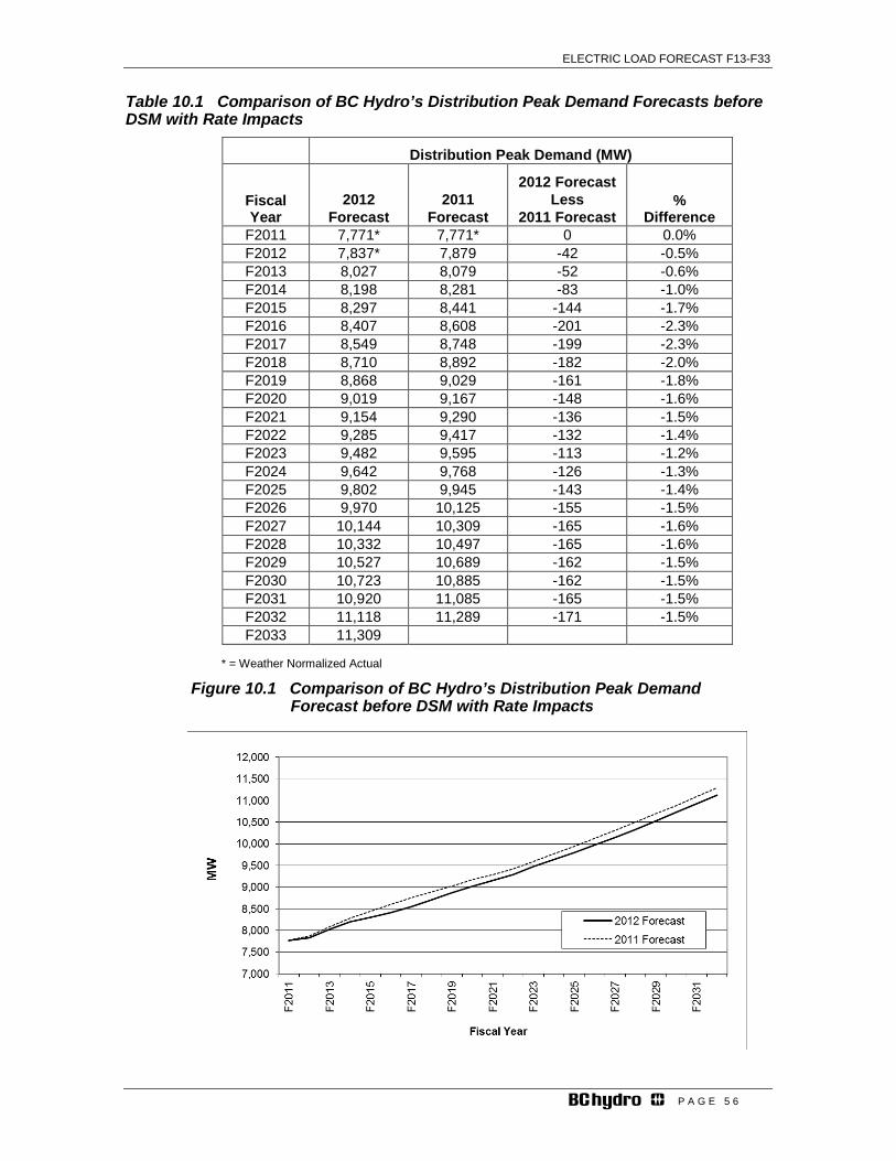
ELECTRIC LOAD FORECAST F13-F33
P A G E 5 6
Table 10.1 Comparison of BC Hydro’s Distribution Peak Demand Forecasts before DSM with Rate Impacts
Distribution Peak Demand (MW)
Fiscal Year
2012 Forecast
2011 Forecast
2012 Forecast Less
2011 Forecast
%
Difference F2011 7,771* 7,771* 0 0.0% F2012 7,837* 7,879 -42 -0.5% F2013 8,027 8,079 -52 -0.6% F2014 8,198 8,281 -83 -1.0% F2015 8,297 8,441 -144 -1.7% F2016 8,407 8,608 -201 -2.3% F2017 8,549 8,748 -199 -2.3% F2018 8,710 8,892 -182 -2.0% F2019 8,868 9,029 -161 -1.8% F2020 9,019 9,167 -148 -1.6% F2021 9,154 9,290 -136 -1.5% F2022 9,285 9,417 -132 -1.4% F2023 9,482 9,595 -113 -1.2% F2024 9,642 9,768 -126 -1.3% F2025 9,802 9,945 -143 -1.4% F2026 9,970 10,125 -155 -1.5% F2027 10,144 10,309 -165 -1.6% F2028 10,332 10,497 -165 -1.6% F2029 10,527 10,689 -162 -1.5% F2030 10,723 10,885 -162 -1.5% F2031 10,920 11,085 -165 -1.5% F2032 11,118 11,289 -171 -1.5% F2033 11,309
* = Weather Normalized Actual
Figure 10.1 Comparison of BC Hydro’s Distribution Peak Demand Forecast before DSM with Rate Impacts

ELECTRIC LOAD FORECAST F13-F33
P A G E 5 7
10.3.2 Transmission Peak Figure 10.2.1 and Table 10.2.1 compare the 2012 and 2011 BC Hydro total coincident transmission peak forecast before DSM and with rate impacts, and excluding LNG. The transmission coincident peak forecast is substantially lower in the 2012 Forecast compared to last year. In the short-term, the current transmission peak forecast is below the 2011 Forecast due to a several factors consistent with the transmission energy forecast. This includes reduced forestry related peak demand from revised production and specific mill forecasts, and new in-service date information on peak demand requirements for new mines expected over the five years. Additionally the near-term peak demand from oil and gas sector is lower. Over the medium to long-term, the transmission peak forecast is lower than last year forecast driven by a decrease in the mining sector energy and peak forecast. The uncertainty in global economic conditions, lower commodity outlook and the tightening of financing conditions for many mining companies have resulted in lower probabilities for new projects and pushed out start dates for several mines. While expectations for mining peak loads are considerably lower over the medium to long term, the oil and gas producer load forecasts (energy and peak demands) are somewhat high over this period. For further details, on long term gas producers and oil pipeline loads see Appendix 4.
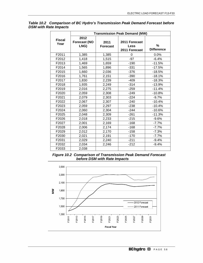
ELECTRIC LOAD FORECAST F13-F33
P A G E 5 8
Table 10.2 Comparison of BC Hydro’s Transmission Peak Demand Forecast before DSM with Rate Impacts
Fiscal Year
Transmission Peak Demand (MW) 2012
Forecast (NO LNG)
2011
Forecast
2011 Forecast
Less 2011 Forecast
% Difference
F2011 1,385 1,385 0 0.0% F2012 1,418 1,515 -97 -6.4% F2013 1,469 1,659 -190 -11.5% F2014 1,565 1,896 -331 -17.5% F2015 1,660 2,036 -376 -18.5% F2016 1,761 2,151 -390 -18.1% F2017 1,830 2,239 -409 -18.3% F2018 1,935 2,249 -314 -13.9% F2019 2,016 2,275 -259 -11.4% F2020 2,059 2,308 -249 -10.8% F2021 2,079 2,303 -224 -9.7% F2022 2,067 2,307 -240 -10.4% F2023 2,059 2,297 -238 -10.4% F2024 2,060 2,304 -244 -10.6% F2025 2,048 2,309 -261 -11.3% F2026 2,018 2,233 -215 -9.6% F2027 2,001 2,169 -168 -7.7% F2028 2,006 2,174 -168 -7.7% F2029 2,012 2,170 -158 -7.3% F2030 2,021 2,191 -170 -7.7% F2031 2,029 2,240 -211 -9.4% F2032 2,034 2,246 -212 -9.4% F2033 2,038
Figure 10.2 Comparison of Transmission Peak Demand Forecast before DSM with Rate Impacts
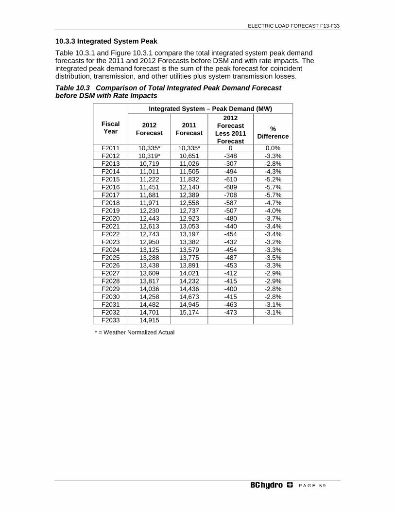
ELECTRIC LOAD FORECAST F13-F33
P A G E 5 9
10.3.3 Integrated System Peak Table 10.3.1 and Figure 10.3.1 compare the total integrated system peak demand forecasts for the 2011 and 2012 Forecasts before DSM and with rate impacts. The integrated peak demand forecast is the sum of the peak forecast for coincident distribution, transmission, and other utilities plus system transmission losses. Table 10.3 Comparison of Total Integrated Peak Demand Forecast before DSM with Rate Impacts
Fiscal Year
Integrated System – Peak Demand (MW)
2012 Forecast
2011 Forecast
2012 Forecast
Less 2011 Forecast
%
Difference
F2011 10,335* 10,335* 0 0.0% F2012 10,319* 10,651 -348 -3.3% F2013 10,719 11,026 -307 -2.8% F2014 11,011 11,505 -494 -4.3% F2015 11,222 11,832 -610 -5.2% F2016 11,451 12,140 -689 -5.7% F2017 11,681 12,389 -708 -5.7% F2018 11,971 12,558 -587 -4.7% F2019 12,230 12,737 -507 -4.0% F2020 12,443 12,923 -480 -3.7% F2021 12,613 13,053 -440 -3.4% F2022 12,743 13,197 -454 -3.4% F2023 12,950 13,382 -432 -3.2% F2024 13,125 13,579 -454 -3.3% F2025 13,288 13,775 -487 -3.5% F2026 13,438 13,891 -453 -3.3% F2027 13,609 14,021 -412 -2.9% F2028 13,817 14,232 -415 -2.9% F2029 14,036 14,436 -400 -2.8% F2030 14,258 14,673 -415 -2.8% F2031 14,482 14,945 -463 -3.1% F2032 14,701 15,174 -473 -3.1% F2033 14,915
* = Weather Normalized Actual
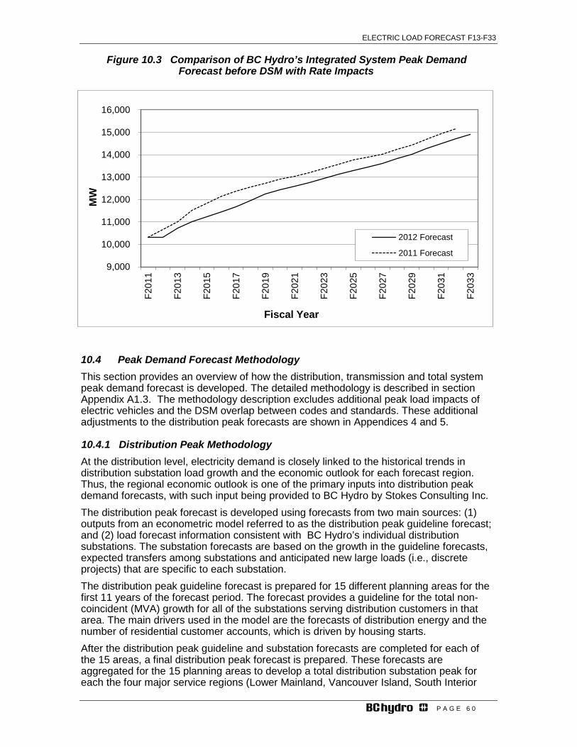
ELECTRIC LOAD FORECAST F13-F33
P A G E 6 0
Figure 10.3 Comparison of BC Hydro’s Integrated System Peak Demand Forecast before DSM with Rate Impacts
10.4 Peak Demand Forecast Methodology This section provides an overview of how the distribution, transmission and total system peak demand forecast is developed. The detailed methodology is described in section Appendix A1.3. The methodology description excludes additional peak load impacts of electric vehicles and the DSM overlap between codes and standards. These additional adjustments to the distribution peak forecasts are shown in Appendices 4 and 5.
10.4.1 Distribution Peak Methodology At the distribution level, electricity demand is closely linked to the historical trends in distribution substation load growth and the economic outlook for each forecast region. Thus, the regional economic outlook is one of the primary inputs into distribution peak demand forecasts, with such input being provided to BC Hydro by Stokes Consulting Inc. The distribution peak forecast is developed using forecasts from two main sources: (1) outputs from an econometric model referred to as the distribution peak guideline forecast; and (2) load forecast information consistent with BC Hydro’s individual distribution substations. The substation forecasts are based on the growth in the guideline forecasts, expected transfers among substations and anticipated new large loads (i.e., discrete projects) that are specific to each substation. The distribution peak guideline forecast is prepared for 15 different planning areas for the first 11 years of the forecast period. The forecast provides a guideline for the total non-coincident (MVA) growth for all of the substations serving distribution customers in that area. The main drivers used in the model are the forecasts of distribution energy and the number of residential customer accounts, which is driven by housing starts. After the distribution peak guideline and substation forecasts are completed for each of the 15 areas, a final distribution peak forecast is prepared. These forecasts are aggregated for the 15 planning areas to develop a total distribution substation peak for each the four major service regions (Lower Mainland, Vancouver Island, South Interior
9,000
10,000
11,000
12,000
13,000
14,000
15,000
16,000
F201
1
F201
3
F201
5
F201
7
F201
9
F202
1
F202
3
F202
5
F202
7
F202
9
F203
1
F203
3
MW
Fiscal Year
2012 Forecast
2011 Forecast

ELECTRIC LOAD FORECAST F13-F33
P A G E 6 1
and Northern Region). Regional power factors and coincidence factors are applied to aggregated forecasts to produce four regional coincident distribution peak forecasts in MW. For the second 10 years of the forecast period, the distribution peak forecast for each region is derived using the growth rate in the distribution energy sales forecast. A total BC Hydro distribution substation peak forecast is prepared as a coincident sum of the four regional distribution peak forecasts. The equations and other details describing the development of the distribution peak forecast are contained in Appendix A1.3.
10.4.2 Transmission Peak Methodology The transmission peak demand forecast is prepared on a customer-by-customer account basis for the entire forecast period. Individual transmission customer forecasts are developed using market intelligence from BC Hydro’s key account managers, historical peak demand trends, reports on industry outlooks, plus production and intensity estimates. These forecasts are aggregated into regional peak forecasts (i.e.; a total transmission peak demand forecast) for each of the four main service regions. Regional coincidence factors and power factors are applied to each of these total regional peak forecasts to establish regional coincident transmission peak forecasts. A total BC Hydro transmission peak demand forecast is prepared as a coincident sum of the four regional transmission peak forecasts. The equations and other details describing the development of the transmission peak forecast are located in Appendix A1.3.

ELECTRIC LOAD FORECAST F13-F33
P A G E 6 2
10.4.3 Integrated System Peak Forecast Methodology A total system peak demand forecast is prepared as the sum of the total coincident distribution peak, total coincident transmission peak, peak demands for other utilities and total system transmission losses. The coincident distribution peak and transmission peak forecasts are informed from the individual substation forecasts. As such, the substation demands at the distribution and transmission level are counted once in developing the total system peak forecast. The system transmission losses are assumed as 7.5 percent of the total system peak demand forecast. The system peak demand forecast is prepared for the BC Hydro’s domestic system and the total integrated system. The domestic peak demand is the sum of the total domestic distribution and transmission peaks, the peak demand of the City of New Westminster and system transmission losses. The integrated system peak demand is the domestic peak demand plus the peak demands from the other utilities (i.e., Seattle City Light and FortisBC) and system transmission losses.
10.5 Risks and Uncertainties Uncertainties and risks in the peak demand forecast come from several factors such as the assumptions on the growth of forecast drivers and model parameters to the anticipated normal weather assumption and its impact on the peak demand. Upward Pressure on Peak Demand:
• The strong housing demand in B.C. as evidenced by residential accounts growth; • Stronger regional growth; • Continued high commodity prices and market demand for B.C.’s exports; and • Increased number of discrete distribution-connected spot loads.
Downward Pressure on Peak Demand: • Slowdown in the housing market with more vacancies and less development than
expected; • Lower commodity prices and a slowdown in the U.S. or Asian economies; and • Pine beetle infestation resulting in additional forestry sector challenges.
BC Hydro quantifies the overall uncertainty in the peak demand using the results of the Monte Carlo uncertainty model as described in Chapter 5.

ELECTRIC LOAD FORECAST F13-F33
P A G E 6 3
11 Glossary Accrued Sales are an estimate of electricity delivered within a specific month. Most
customer meters are not read at every month-end, so the amount of electricity delivered in a month is not known precisely. In accordance with GAAP, monthly accrued sales are used for monthly financial reporting.
Backcasting Estimating econometric or other models over a historical time period and comparing the predictions of the models to actual results over the same time period.
Billed Sales The amount of electricity billed. Because bills are produced after the electricity has been delivered, monthly billed sales lag monthly delivery of electricity.
Binary Variable is a variable whose value is either zero or one. Binary variables are often used as independent variables in regression models in order to account for events that either occur or do not occur. In this latter context, binary variables are often referred to as “dummy variables” in regression.
Calibration Estimating econometric or other models over a historical time period. Coincidence Factor A ratio reflecting the relative magnitude of a region’s (or customer’s
or group of customers’) demand at the time of the system’s maximum peak demand to the region’s (or customer’s or group of customers’) maximum peak demand.
Commercial Output Commercial output focuses on the provisions of services in the economy and so includes such things as public administration, insurance agents, bankers, wholesale and retail trade, food services, accommodation provisions etc.
Consumer Price Index (CPI) An inflation index calculated by comparing the price of a typical bundle of goods in the year in question to the price of the same goods in a set reference year.
Cooling Degree Day (CDD) is a measure of warmness, defined by the number of degrees above 18 degrees Celsius for the average daily temperature. CDDs are drivers of utility air-conditioning electricity loads.
Demand-Side Management (DSM) Activities that occur on the demand side of the revenue meter and are influenced by the utility. DSM activities result in a change in electricity sales. Past DSM savings include incremental load displacement and energy efficiency savings. Note that BC Hydro’s historical sales include the impact of DSM savings realized up to that year.
Design Temperature Rolling average of the coldest daily average temperature over the most recent 30 years
Distribution voltage customer A BC Hydro customer who receives electricity via distribution lines that operates at lower voltages (60 kV and less).
Domestic System Peak includes the peak requirements for BC Hydro’s distribution and transmission customers in its service territory; sales to the City of New Westminster and system transmission and distribution losses.
Econometric Modelling The use of statistical techniques, typically regression analysis of time-series and/or cross-sectional data, to detect statistically verifiable relationships, coherent with economic theory, between an explained variable (e.g. electricity consumption) and explanatory variables (e.g. industry output, prices of alternative energy inputs and GDP).
Elasticity The proportionate change in a dependent variable (e.g. electricity consumption) divided by the proportionate change in a specified independent variable (e.g. electricity price). A dependent variable is highly elastic with respect to a given independent variable if the calculated elasticity is much greater than one. The dependent variable is inelastic if the elasticity is less than one.
ELECTRIC LOAD FORECAST F13-F33
P A G E 6 4
End-use Model A model used to analyze and forecast energy demand, which focuses on the end uses or services provided by energy. Typical end uses are lighting, process heat and motor drive. For a given industry, the model estimates the influence of prices and technological change on the evolution of the secondary energy inputs required to satisfy the industry's end uses over time.
Energy The amount of electricity delivered or consumed over a certain time period, measured in multiples of watt-hours. A 100-watt bulb consumes 200 watt-hours in two hours.
Energy Efficiency Is the ratio of the energy service delivered from a process or piece of equipment to the energy input. Energy efficiency is a dimensionless number, with a value between 0 and 1 or, when multiplied by 100, is given as a percentage.
EV Electric Vehicle GAAP Generally Accepted Accounting Principles Gigawatt-hour (GWh) A measure of electrical energy, equivalent to one million kilowatt-
hours. (See Units of Measure.) Gross Domestic Product (GDP) A measure of the total flow of goods and services
produced by the economy over a specified time period, normally a year or quarter. It is obtained by valuing outputs of goods and services at market prices (alternatively at factor cost), and then aggregating the total of all goods and services.
Heating Degree Day (HDD) Is a measure of coldness, defined by the number of degrees below 18 degrees Celsius for the average daily temperature. HDDs are drivers of utility space heating electricity loads.
Integrated System That portion of the BC Hydro electricity system which is connected as one whole by a high voltage transmission grid.
Integrated System Peak includes the peak requirements for BC Hydro’s distribution and transmission customers in its service territory; sales to Other Utilities, which includes Seattle City Light, New Westminster, FortisBC and Hyder Alaska (Tongass Power and Light Co. Inc.); and system transmission and distribution losses.
Intensity A unitized measure of energy consumption, typically in kilowatt-hours per unit of stock. For example, kWh per account in the residential sector or kWh per unit of production in the industrial sector.
Kilowatt-hour (kWh) A measure of electrical energy, equivalent to the energy consumed by a 100-watt bulb in 10 hours. (See Units of Measure)
Liquefied Natural Gas (LNG) is natural gas that has been converted temporarily to liquid form for ease of storage or transport. This process involves refrigeration, and requires no chemical transformations.
Load The total amount of electrical power demanded by the utility's customers at any given time, typically measured in megawatts.
Load Displacement Projects that involve the installation of self-generation facilities at customer sites, with the electricity generated being used on-site by the customer, with a resultant decrease in the purchase of electricity from BC Hydro.
Megawatt (MW) A unit used to measure the capacity or potential to generate or consume electricity. One MW equals one million watts. (See Units of Measure.)
Megawatt-hour (MWh) A measure of electrical energy, equivalent to 1,000 kWh. (See Units of Measure)
Monte Carlo Method A technique for estimating probabilities involving the construction of a model and the simulation of the outcome of an activity a large number of times.

ELECTRIC LOAD FORECAST F13-F33
P A G E 6 5
Random sampling techniques are used to generate a range of outcomes. Probabilities are estimated from an analysis of this range of outcomes.
Megavolt-Amps (MVA) – a unit of apparent power, which is real power in MW, divided by power factor.
Natural conservation The increase in energy efficiency that would occur in the absence of any utility-induced demand-side management program, all other things being equal.
Non-coincident In general is the magnitude of a region’s (or customer’s or group of customers’) demand at the time of its peak.
Non-Integrated Area (NIA) Non-integrated facilities refer to generating facilities that are not connected to the system, located in remote areas of the province
Normalization The correction of actual customer sales and peak demand for factors such as unusually warm or cold weather.
Ordinary Least Squares (OLS) is a method of estimating parameters to minimize the sum of squares errors in a regression model.
Price Elasticity of Demand The percentage change in quantity demanded, divided by the percentage change in price that caused the change in quantity demanded.
Real Price Increases that have been adjusted for changes in prices of all goods. The nominal price of an item may rise by 10 per cent over a year, but inflation (and assumed wages) may have risen by seven per cent over the same time period. Therefore the effective price increase faced by the consumer is close to three per cent. It is necessary to deflate current prices by an appropriate inflation index (the CPI in Canada) to convert money values to constant prices or real terms.
Reference Forecast before DSM and Rate Impacts is the energy and peak demand forecast developed under the current methodology. It is developed under the assumption that electricity rates increase at the rate of inflation and normal weather conditions.
Region A geographical sub-division of the BC Hydro service area used for Load Forecast purposes. Four regions exist: Lower Mainland, Vancouver Island, South Interior and the Northern Region.
Stock A quantity representing a number of energy consuming units. For example, in the residential sector, stock is the number of accounts or housing units; in the commercial sector, stock is represented by the floor area of commercial building space.
System Coincident Peak Demand The greatest combined demand of all BC Hydro customers faced by the generation system during a given fiscal year.
Transmission Voltage Customer A BC Hydro customer that is supplied its electricity via high-voltage transmission lines (60 kV or above).
Units of Measure The large amounts of electricity generated and consumed on a system-wide basis are discussed in multiples of the basic units of watt and watt-hours. Kilowatts and megawatts are used to measure power, and kilowatt-hours, megawatt-hours, and gigawatt-hours are used to measure energy. The equivalence is: 1 kilowatt (kW) = 1,000 watts 1 megawatt (MW) = 1,000 kilowatts or 1 million watts 1 kilowatt-hour (kWh) = 1,000 watt-hours 1 megawatt-hour (MWh) = 1,000 kilowatt-hours or 1 million watt-hours 1 gigawatt-hour (GWh) = 1,000 megawatt-hours or 1 billion watt-hours

ELECTRIC LOAD FORECAST F13-F33
P A G E 6 6
Appendix 1 Forecast Processes and Methodologies There are a number of key components to the demand and sales forecast: the residential forecast; the commercial forecast (distribution and transmission voltage), the industrial forecast (distribution voltage and transmission voltage), and the regional and system peak forecasts. The peak forecast includes the distribution voltage and transmission voltage peak demands. This section covers the methodology used for these forecast components.
A1.1. Statistically Adjusted Forecast Methodology Distribution BC Hydro forecasts residential and commercial distribution sales9 by using the Statistically Adjusted End-Use model (SAE). This model incorporates end-use information, economic data, weather data and market data to construct regional forecasts. The statistically adjusted end-use modeling framework begins by defining energy use (Usem) in year and month (m) as the sum of energy used by heating equipment (Heatm), cooling equipment (Coolm), and other equipment (Otherm). Formally,
(A1.1) mmmm CoolHeatUSE Other++=
Equation (A1.1) can be shown in a regression form, as shown below in (A1.2):
(A1.2) mmmmm XOtherbXCoolbXHeatbaUSE ε+×+×+×+= 321
Here, XHeatm, XCoolm, and XOtherm are explanatory variables constructed from end-use information, economic drivers, dwelling data and weather data and mε is the error term for the regression. The estimated model can then be thought of as a statistically adjusted end-use model, where the estimated coefficients are the adjustment factors or the relative contribution by the major end uses to the total consumption. The equations used to construct these X-variables are simplified end-use models, and the X-variables are the estimated usage levels for each of the major end uses based on the end use models. BC Hydro also includes other variables in equation A1.2. Other variables include binary variables to account for migration of accounts between customer classes. In addition seasonal variables are included. Constructing XHeat. Space heating energy is specified to depend on the following types of variables:
• Heating degree days (weather), • Heating equipment saturation levels (fraction of building stock for the
commercial sector), • Assumptions about heating equipment operating efficiencies, • Average number of days in the billing cycle for each month,
9 The commercial sales are composed of commercial general rate class, transmission and BC Hydro Own Use, Irrigation, Street-lighting. The SAE model is used to forecast the sales for the commercial general rate class. The sales forecast for BC Hydro Own Use, Irrigation, and Street-lighting is done using historical sales data and trend analysis. The SAE models are calibrated over a 10 year rolling period.

ELECTRIC LOAD FORECAST F13-F33
P A G E 6 7
• Economic variables include employment, retail sales and commercial output. The heating variable is represented as the product of an annual equipment index and a monthly usage multiplier. That is,
(A1.3) mmm HeatUseHeatIndexXHeat ×=
where, XHeatm is estimated heating energy use in a year (y) and month (m), HeatIndexy is the annual index of heating equipment in the year (y), and HeatUsem is the monthly usage multiplier. The sub equation for HeatIndexm in (A1.3) is: Where, y means year, e refers to the category of space heating, Share means saturation level of space heating, Eff means efficiency level of space heating based on Energy Information Administration (EIA) data The sub equation for XHeatUsem in (A1.3) is:
HeatUsem = Commercial GDPIndexβ1m × EmploymentIndexβ2m × RetailSalesIndexβ3m × Heating Degree Days Indexm.
Where m refers to month specific values and the β values are the elasticity that apply to the various regional economic indices above (i.e., commercial GDP, employment, and retail sales) and small commercial sales. The residential SAE model some of the economic drivers are different to the commercial sector economic drivers. The residential sector drivers include: disposable income, household sizes and weather as non-economic drivers. The economic indices for each variable are developed based on a 12 month rolling average of the economic variable weighted by its average monthly value in the last historical year. The heating equipment index (HeatIndex) depends on the space heating equipment saturation levels normalized by average operating efficiency levels. As a result, the index will increase over time if there are increases in heating equipment saturation levels, and will decrease over time if there are improvements in equipment and building efficiency levels. Heating system usage levels (HeatUse) are driven on a monthly basis by economic variables and non-economic factors, such as weather (Heating Degree Days). Constructing XCool. The explanatory variable for cooling loads is constructed in a similar manner. The amount of energy used by cooling systems depends on the following types of variables:
• Cooling degree days (weather), • Cooling equipment saturation levels (fraction of building stock for the
commercial sector), • Assumptions about cooling equipment operating efficiencies, • Average number of days in the billing cycle for each month,
×= ∑BaseYear
BaseYear
y
y
ngspaceheatiBaseYearey
EffShare
EffShare
gyEndUseEnerHeatIndex ,

ELECTRIC LOAD FORECAST F13-F33
P A G E 6 8
• Economic variables include employment, retail sales and commercial output.
The cooling variable is represented as the product of an equipment-based index and monthly usage multiplier. That is,
(A1.4) mmm CoolUseCoolIndexXCool ×=
where, XCoolm is estimated cooling energy use in a year and month (m),
CoolIndexy is an index of cooling equipment for the year (y), and CoolUsem is the monthly usage multiplier.
As with space heating, the cooling equipment index (CoolIndex) depends on the cooling equipment saturation levels normalized by average operating efficiency levels. As a result, the cooling index will increase over time if there are changes in cooling equipment saturation levels, and will decrease over time if there are improvements in equipment efficiencies or the thermal efficiency of buildings. Space cooling system usage levels (CoolUse) are driven on a monthly basis by several factors, including weather (Cooling Degree Days) and similar economic factors used to develop heating usage. Constructing XOther. Monthly estimates of consumption for non-weather sensitive end uses can be derived in a similar fashion. Non-weather sensitive end-uses include lighting, refrigeration, cooking, clothes washing and drying, entertainment and other miscellaneous equipment. Based on end-use concepts, other sales are driven by:
• Appliance and equipment saturation levels, • Appliance efficiency levels, • Average number of days in the billing cycle for each month, and
• Economic variables include employment, retail sales and commercial output. The explanatory variable for other uses is defined as follows:
(A1.5) mmm OtherUseIndex OtherEqpXOther ×=
The first term on the right hand side of this expression (OtherEqpIndexy) embodies information about appliance saturation and efficiency levels. The second term (OtherUse) captures the impact of changes in economic variables that impact use of other equipment. These economic variables are similar to those used for explaining heating and cooling.
Figure A1.1 below summarized the inputs that are used in the construction of the regression variables (i.e. the predictor variables) for the commercial sector.
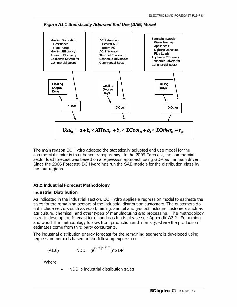
ELECTRIC LOAD FORECAST F13-F33
P A G E 6 9
Figure A1.1 Statistically Adjusted End Use (SAE) Model
The main reason BC Hydro adopted the statistically adjusted end use model for the commercial sector is to enhance transparency. In the 2005 Forecast, the commercial sector load forecast was based on a regression approach using GDP as the main driver. Since the 2006 Forecast, BC Hydro has run the SAE models for the distribution class by the four regions.
A1.2. Industrial Forecast Methodology Industrial Distribution As indicated in the industrial section, BC Hydro applies a regression model to estimate the sales for the remaining sectors of the industrial distribution customers. The customers do not include sectors such as wood, mining, and oil and gas but includes customers such as agriculture, chemical, and other types of manufacturing and processing. The methodology used to develop the forecast for oil and gas loads please see Appendix A3.2. For mining and wood, the methodology follows from production and intensity, where the production estimates come from third party consultants. The industrial distribution energy forecast for the remaining segment is developed using regression methods based on the following expression:
(A1.6) INDD = (eα + β * T
)*GDP Where:
• INDD is industrial distribution sales
Heating SaturationResistanceHeat Pump
Heating EfficiencyThermal EfficiencyEconomic Drivers for Commercial Sector
AC SaturationCentral ACRoom AC
AC EfficiencyThermal EfficiencyEconomic Drivers for Commercial Sector
Saturation LevelsWater HeatingAppliancesLighting DensitiesPlug Loads
Appliance EfficiencyEconomic Drivers for Commercial Sector
HeatingDegreeDays
CoolingDegreeDays
BillingDays
XHeat XCool XOther
mmmmm XOtherbXCoolbXHeatbaUSE ε+×+×+×+= 321
HeatingDegreeDays
HeatingDegreeDays
CoolingDegreeDays
CoolingDegreeDays
BillingDaysBillingDays
XHeatXHeat XCoolXCool XOtherXOther
mmmmm XOtherbXCoolbXHeatbaUSE ε+×+×+×+= 321 mmmmm XOtherbXCoolbXHeatbaUSE ε+×+×+×+= 321
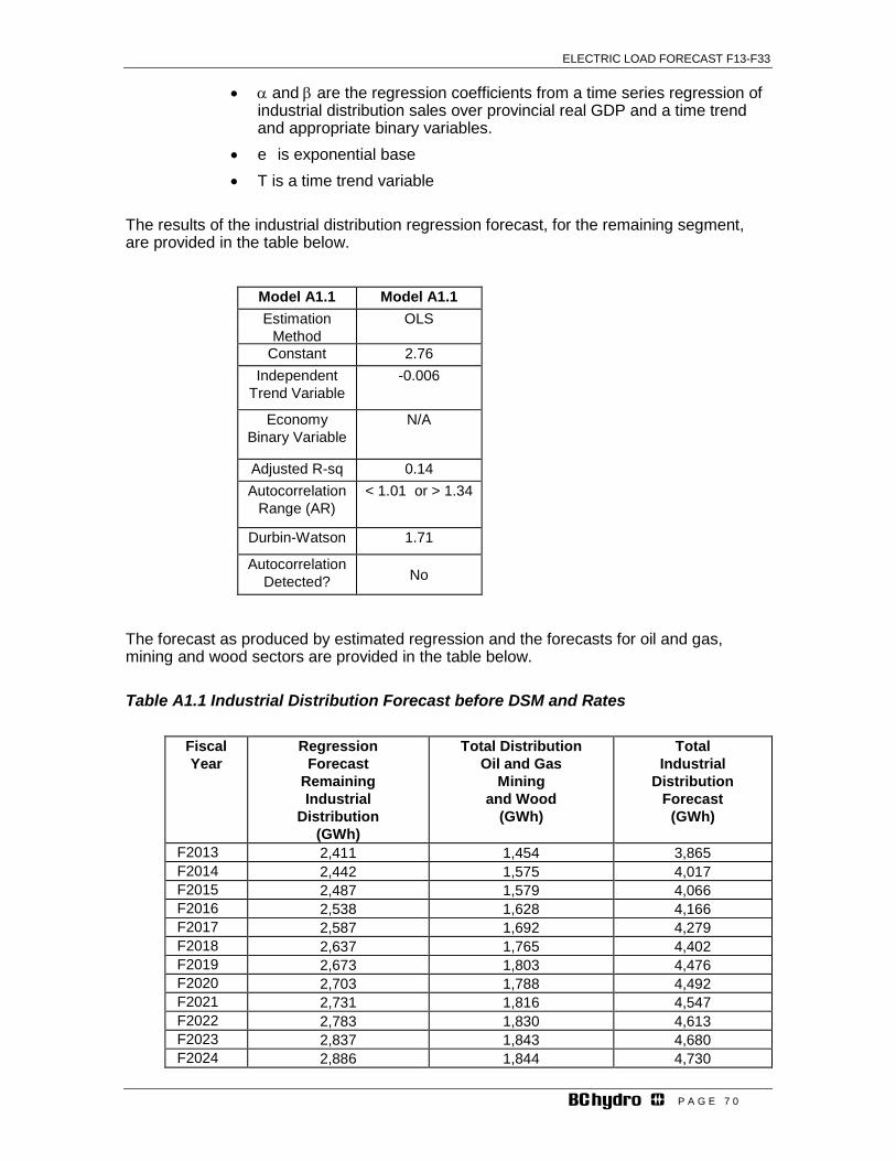
ELECTRIC LOAD FORECAST F13-F33
P A G E 7 0
• α and β are the regression coefficients from a time series regression of industrial distribution sales over provincial real GDP and a time trend and appropriate binary variables.
• e is exponential base • T is a time trend variable
The results of the industrial distribution regression forecast, for the remaining segment, are provided in the table below.
Model A1.1 Model A1.1 Estimation
Method
OLS
Constant 2.76 Independent
Trend Variable -0.006
Economy Binary Variable
N/A
Adjusted R-sq 0.14 Autocorrelation
Range (AR) < 1.01 or > 1.34
Durbin-Watson 1.71
Autocorrelation Detected? No
The forecast as produced by estimated regression and the forecasts for oil and gas, mining and wood sectors are provided in the table below.
Table A1.1 Industrial Distribution Forecast before DSM and Rates
Fiscal Year
Regression Forecast
Remaining Industrial
Distribution (GWh)
Total Distribution Oil and Gas
Mining and Wood
(GWh)
Total Industrial
Distribution Forecast
(GWh)
F2013 2,411 1,454 3,865 F2014 2,442 1,575 4,017 F2015 2,487 1,579 4,066 F2016 2,538 1,628 4,166 F2017 2,587 1,692 4,279 F2018 2,637 1,765 4,402 F2019 2,673 1,803 4,476 F2020 2,703 1,788 4,492 F2021 2,731 1,816 4,547 F2022 2,783 1,830 4,613 F2023 2,837 1,843 4,680 F2024 2,886 1,844 4,730
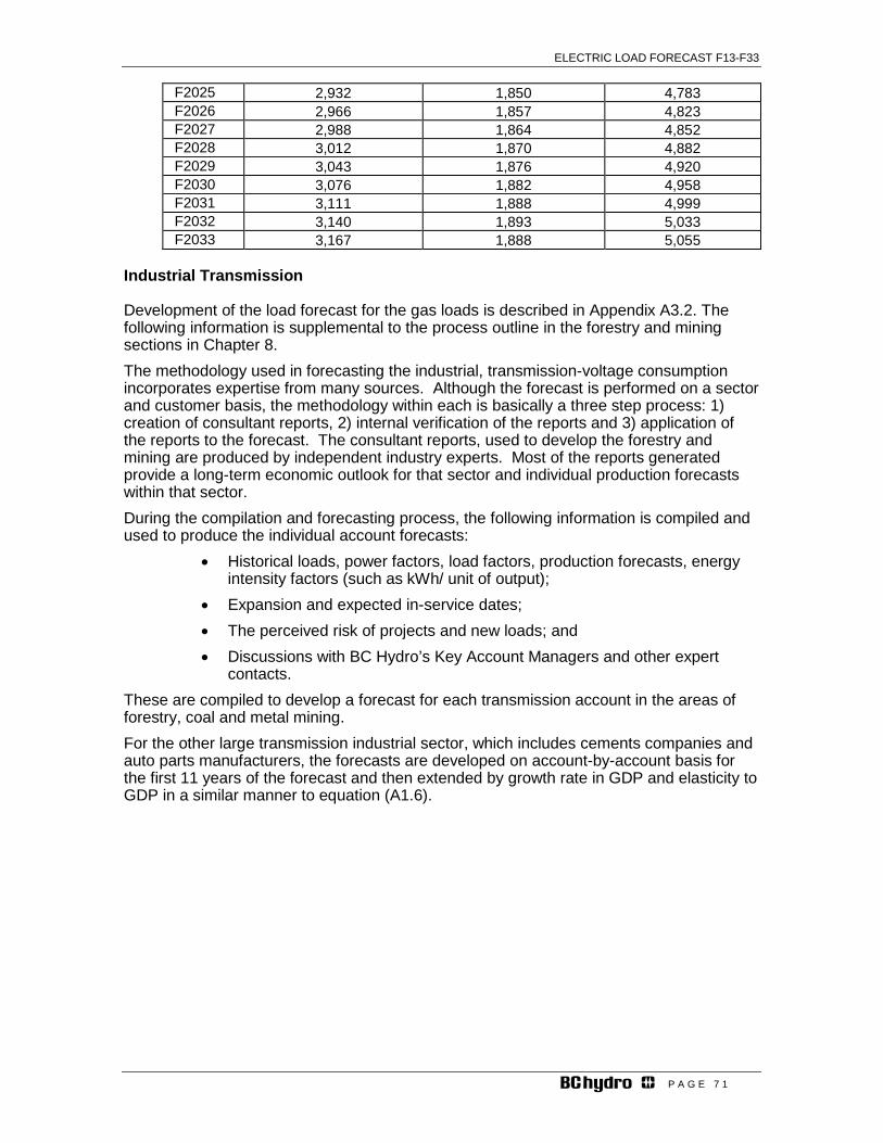
ELECTRIC LOAD FORECAST F13-F33
P A G E 7 1
F2025 2,932 1,850 4,783 F2026 2,966 1,857 4,823 F2027 2,988 1,864 4,852 F2028 3,012 1,870 4,882 F2029 3,043 1,876 4,920 F2030 3,076 1,882 4,958 F2031 3,111 1,888 4,999 F2032 3,140 1,893 5,033 F2033 3,167 1,888 5,055
Industrial Transmission
Development of the load forecast for the gas loads is described in Appendix A3.2. The following information is supplemental to the process outline in the forestry and mining sections in Chapter 8. The methodology used in forecasting the industrial, transmission-voltage consumption incorporates expertise from many sources. Although the forecast is performed on a sector and customer basis, the methodology within each is basically a three step process: 1) creation of consultant reports, 2) internal verification of the reports and 3) application of the reports to the forecast. The consultant reports, used to develop the forestry and mining are produced by independent industry experts. Most of the reports generated provide a long-term economic outlook for that sector and individual production forecasts within that sector. During the compilation and forecasting process, the following information is compiled and used to produce the individual account forecasts:
• Historical loads, power factors, load factors, production forecasts, energy intensity factors (such as kWh/ unit of output);
• Expansion and expected in-service dates; • The perceived risk of projects and new loads; and • Discussions with BC Hydro’s Key Account Managers and other expert
contacts. These are compiled to develop a forecast for each transmission account in the areas of forestry, coal and metal mining. For the other large transmission industrial sector, which includes cements companies and auto parts manufacturers, the forecasts are developed on account-by-account basis for the first 11 years of the forecast and then extended by growth rate in GDP and elasticity to GDP in a similar manner to equation (A1.6).
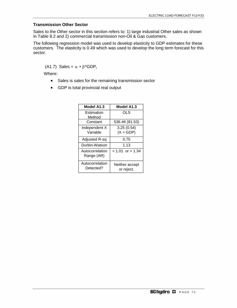
ELECTRIC LOAD FORECAST F13-F33
P A G E 7 2
Transmission Other Sector Sales to the Other sector in this section refers to: 1) large industrial Other sales as shown in Table 8.2 and 2) commercial transmission non-Oil & Gas customers. The following regression model was used to develop elasticity to GDP estimates for these customers. The elasticity is 0.49 which was used to develop the long term forecast for this sector.
(A1.7) Sales = α + β*GDPt Where:
• Sales is sales for the remaining transmission sector • GDP is total provincial real output
Model A1.3 Model A1.3 Estimation
Method
OLS
Constant 536.46 (81.53) Independent X
Variable 3.25 (0.54) (X = GDP)
Adjusted R-sq 0.75 Durbin-Watson 1.13 Autocorrelation
Range (AR) < 1.01 or > 1.34
Autocorrelation Detected?
Neither accept or reject.

ELECTRIC LOAD FORECAST F13-F33
P A G E 7 3
A1.3. Peak Demand Forecast Methodology Figure A1.2 below shows that the bottom-up peak forecast methodology involves several steps for each of the distribution and transmission peak forecasts. The general description of the development stages in system peak forecast is provided following.
Figure A1.2 Peak Demand Forecast Roll-up
The peak demand forecast is built up in three main stages, each incorporating several steps. First stage is the creation of the substation peak in MVA non-coincident10, second, the four main service region peak forecasts in MW are determined on a region coincident basis and third, the system peak in MW on a system coincident basis.
Stage 1: Substation Peak Demand Forecast The substation peak forecast is built up in several sub steps: 1 (a) first the weather normalized peak loads by substation/area and short-term forecasts are developed; 1 (b) second the substation peak forecast guidelines are developed from an econometric model for each planning area; 1(c) third an 11-year substation forecast for each substation is created; and, 1 (d) finally the substation and guideline peak forecast are averaged together. The appropriate equations and description of the sub steps are provided below.
1 (a) Weather Normalized Substation Peak and Short-term Forecast
The equation below is the basis for a linear regression model that estimates the relationship between substation peak demand and temperature:
(A1.8) KVA = α + β*min Where:
• KVA is the metered peak load; and • min is the minimum mean temperature for the coldest day during the
metered period. • α and β are the regression coefficients from a time series regression of
peak substation demands on temperatures.
10 Non-coincident is defined in the glossary.
220 Distribution Substations; 160 Transmission Substations
15 Distribution Planning Areas
System
4 Regions
9 Transmission Planning Areas
Bottom Up DrivenForecasting ProcessDetailed to meet users andplanners needs
220 Distribution Substations; 160 Transmission Substations
15 Distribution Planning Areas
System
4 Regions
9 Transmission Planning Areas
220 Distribution Substations; 160 Transmission Substations
15 Distribution Planning Areas
System
4 Regions
9 Transmission Planning Areas
Bottom Up DrivenForecasting ProcessDetailed to meet users andplanners needs

ELECTRIC LOAD FORECAST F13-F33
P A G E 7 4
Using the estimated regression coefficients, the weather-normalized peak is then calculated based on the design day temperature for that substation11:
(A1.9) NKVA = α + β*designmin
Where:
• NKVA is weather-normalized peak; and • designmin is the design temperature for the substation.
The first step involves estimating a relationship between substation peak demand and temperature and determining weather-normalized substation peak for each substation for the previous winter. This is produced by equation A1.15. The weather normalized substation peak along with historical growth rates of substation peak demands, expected transfers of substation load and expected discrete load additions or closures are used by BC Hydro Distribution planners to prepare a short-term forecast for each substation for the upcoming winter. The first step is completed with an estimate of the weather normalized peak for each substation for the base year or the most recent historical year. 1(b) Distribution Peak Guideline Forecast. In the section sub step, a distribution substation peak guideline forecast is prepared for 15 planning areas for the first 11 years of the forecast period using the following forecasting and (econometric model) equation:
(A1.10) SKit = [α1SFDHTG + α2SFDNON + α3MULTHTG + α4MULNON + α5U35E +
α6O35E] Where:
• SKit is the total substation peak for the ith planning area; • SFDHTG is the number of single-family electrically heated homes; • SFDNON is the number of single-family non-electrically heated homes; • MULTHTG is the number of multi-family electrically heated homes; • MULTNON is the number of multi-family non-electrically heated homes; • U35E is annual energy consumption General under 35 kW; • O35E is annual energy consumption General over 35 kW; • the coefficients α1, α2, α3, and α4 are kW contribution to the distribution
peak per dwelling in area i, for the four dwelling types under normal temperature conditions; and the coefficients, α5 and α6 represent the increase in peak demand due to a one-kWh increase in the General rate class Under 35 and Over 35 kW energy consumption. The forecasting equation for the distribution peak guideline model is provided in equation A1.18. The guideline forecast provides the expected total substation growth from the base year for each planning area. The
11 A regression model using non-linear variables was also used for weather normalization.

ELECTRIC LOAD FORECAST F13-F33
P A G E 7 5
drivers of the guideline forecast are based on regional economic information such as housing starts and employment. The guideline forecast is provided to BC Hydro Distribution planners from Market Forecast without adjustments for specific capacity additions or transfers.
1(c) Long-term Substation Forecast
In the third sub-step, an eleven-year substation peak forecast is prepared for each substation using the guidelines, trends in substation growth, forecast load transfers between substations and larger substation load additions. During this step, BC Hydro planners may have additional and information or revised information from field engineers on expected increases or decreases on discrete customer loads as well as operational requirements for substations. This new information, along with the impact of the guideline forecast, may result in a change to the initial short-term forecast for each substation forecast from the first step. The long-term forecasts for each substation are summed up to fifteen planning region totals. These are the total long-term substation forecasts for each planning region.
1(d) Average of Long-term Substation Forecast and Guideline Forecast The fourth sub step is the calculation of the blending or averaging of the long-term substation forecast and the guideline forecast for each of the 15 planning areas. Prior to the forecasts being averaged, the long-term substation peak forecast and the guideline are aggregated from 15 planning areas into four regional total substation forecasts. These sets substation forecasts (i.e. the long-term substation forecast and the peak guideline forecast) are then averaged together for each of the four service regions based on the following equation:
(A1.11) PKit = Σit SKitGuideline + SKi Substation Forecast
Stage 2: Regional Peak Forecast The regional peak is forecast developed using:
(A1.12) RPKjt = Σj [PKit*DCFj*PFj + TPj*TCFj*PFj + OPj*OCFj] Where:
• DCF is the regional distribution peak coincidence factor; • PF is the regional power factor for distribution and transmission; • TP is the transmission peak; this is the aggregate of the transmission
account peak forecast in each service region. • TCF is the transmission coincident factor; • OP is the other utility peak sales; • OCF is the other utility coincident factor; and • PK is the weighted average distribution substation forecast
A transmission peak forecast is prepared for each commercial and industrial transmission account using a bottom-up approach. This involves using the historical peak data, information from Key Account Managers and market information and industry reports.

ELECTRIC LOAD FORECAST F13-F33
P A G E 7 6
Stage 3: System Coincident Peak Forecast Finally, system coincident peak is created as the sum of coincidence-adjusted regional peaks and it includes transmission losses:
(A1.13) SPK = (1 + TL)*Σj RPKjt *SCFj
Where:
• TL is the transmission loss factor; and • SCF are the system coincidence factors for each of the four regions.

ELECTRIC LOAD FORECAST F13-F33
P A G E 7 7
Appendix 2 - Monte Carlo Methods
This Appendix describes the Monte Carlo model that is used to assess the uncertainty associated with BC Hydro's Load Forecast. The description includes a discussion of the methodology, assumptions and parameters of the model. Load forecasting involves considerable uncertainty. The demand for electricity depends on a large number of factors which fluctuate widely with time and which are difficult to measure. Some of these factors include population, gross domestic product, weather, technology, energy conservation programs (DSM), alternate energy source options, the business climate experienced by major customers and the changing tastes and customers. The challenge of assessing the uncertainty of the load forecast is to quantify the way in which uncertainty in the major causal factors flows through to impact the resultant load. To quantify load forecast uncertainty, BC Hydro uses a Monte Carlo model and Monte Carlo simulation techniques. The model and simulation analysis proceeds as follows: • First, several major input variables or causal factors are identified. These are:
economic growth (measured by GDP); price of electricity (electricity rates); weather (measured by heating degree days) and elasticity of load (with respect to GDP and BC Hydro electricity rates). In addition to the major causal factors, uncertainty for residual load impacts, Electrical Vehicles and Load Forecast DSM/Integration overlap with codes and standards are included in the model.
• Second, probability distributions are assigned to each input variable. A model represented by a mathematical relationship between the input variable and the output variables is determined for each sector and the overall load.
• Third, a large number of random samples are taken from the input probability distributions. The mathematic model is used, with each sample as input, to calculate a large number of simulations of the output variables. These simulations are used to construct probability distributions for the output variables.
The model perturbs the Reference forecast for each sector by calculating the impact factors for each of the causal factors and other uncertainty variables. The impact factors are random variables shown in the equations below. For the 2012 forecast, each of the sectors - Residential, Commercial and Industrial – have separate formulas to which their respective Reference forecast is perturbed by separate impact factors. As such the Monte Carlo model has two major components; the energy demand model for the residential and general service sector and the energy demand model for the transmission sector. Previously, the same methodology and essentially the perturbation formula were applied to all the sectors. As for peak demand, the probability distribution for the overall system peak demand is generated using an overall system load factor the energy model. The model is implemented in Microsoft EXCEL augmented with Palisade Corporation’s @RISK software. The energy demand model for the residential, small commercial and industrial sector is the following equation:
(A2.1) Ut
Wt
Gt
Pttt IIIIEE 0=
The energy demand model for the transmission sector, which is most of the overall industrial sector, is the following equation:
(A2.1a) St
Pttt IIEE 0=
ELECTRIC LOAD FORECAST F13-F33
P A G E 7 8
Here Et is perturbed energy demand, 0Et is base case or Reference energy demand, and the major impact factors are identified by their superscripts; P for electricity price (rates), G for GDP, W for weather, U for residual load uncertainty. For the transmission sector the
StI is a new impact factor developed for the forestry, oil and gas, mining and remaining
portions of the transmission load The equation S
tI is as follows: (A2.1b) S
tI = StE0 + ( S
tE0 - StE )
Where, S stands for forestry, oil and gas, mining and remaining transmission sectors, S
tE0is the Reference forecast for those sectors and S
tE is a randomly drawn forecast for those sectors from a triangular distribution. The following describes the impact factors for the major causal factors and other variables in more detail. Impact of GDP Uncertainty: This applies to the residential and general service loads and correlation with the transmission loads. In order to assess the impact of uncertainty in future GDP, the base case GDP is perturbed. The base case GDP is denoted by 0Gt and the perturbed GDP is denoted by Gt . The perturbed GDP starts off being equal to the base case GDP in the first year. It then grows at a growth rate equal to the base case GDP growth rate ( 0gt ) plus a random perturbation growth rate ( gt ). This random perturbation is a normally distributed random variable with zero mean and a standard deviation of 1.70%. That is:
(A2.2) gt ∼ N(0,1.70%) The perturbed GDP is calculated by:
(A2.3.) Gt = Gt-1 [ 1 + 0gt + gt ] . The impact factor for GDP is then given by the following equation:
(A2.4) IGt = exp( α ln(Gt / 0Gt )) = ( Gt / 0Gt )α
where α0 is the elasticity of load with respect to GDP. Impact of Price Uncertainty: (BC Hydro electricity rates): This applies to all major sector loads. The calculation of the impact factor for price changes ( IP
t ) is treated similarly. A random variable, the perturbed price Pt , is calculated starting from the base case price 0Pt . The perturbed price starts out being equal to the base case price in the initial year. It then grows at a rate equal to the base case growth rate plus a random perturbation. In the model, the random perturbation has a triangular distribution with parameters (-2.5%, 0, +2.5%). However, unlike the case of GDP, the impact of price change is assumed to take place on a cumulative basis. Impact of Elasticity Uncertainty: Table A2.1 gives the elasticity parameters and distributions around the elasticity used in the current Monte Carlo model. This elasticity are part of the price and GDP impact factors for the respective sectors.
ELECTRIC LOAD FORECAST F13-F33
P A G E 7 9
Table A2.1. Elasticity Parameter for Monte Carlo Model
Mean Probability Distribution (a,b,c) Price Elasticity Residential Commercial and Industrial General Service Transmission
-0.05 -0.05 -0.05
Triangular (-0.075, -0.05, -0.025) Triangular (-0.075, -0.05, -0.025) Triangular (-0.075, -0.05, -0.025)
GDP Elasticity Residential Commercial and Industrial General Service.
0.670 0.780
Triangular (0.470, 0.670, 0.870) Triangular (0.580, 0.780, 0.980)
In Table A2.1, Triang(a,b,c) refers to a probability distribution known as a triangular distribution because its graph is a triangle. This distribution is zero for values of its random variable less than a or greater than c. It has a maximum (most probable) value at b. Impact of Residual Uncertainty in Load: This factor incorporates the effect on load of other factors such as changes in technology, consumer taste, household structure, business type, and inter-regional differences. This applies to the residential and general service load. The residual error factor starts out at 1.00 in the base year and grows at a rate that is, in each year, a random variable with the triangular distribution. The impact factor is defined by the following equations:
(A2.5) IUt = IUt-1 ( 1 + gUt) IU0 = 1
where gUt denotes a random variable with a triangular distribution. Again, the @RISK
software allows the specification of probability distributions in the model. Impact of Weather: Variations in weather are an important source of uncertainty in load. This applies to the residential and to a lesser extend the commercial general service loads. The weather impact is most important for the residential and commercial loads, so weather impact is modeled only for these sectors. In British Columbia, the impact of cold weather on residential heating load is the most important weather effect and is modeled using heating degree days (HDD). HDD is an indicator of how much energy is needed to heat housing up to a comfortable temperature. BC Hydro’s summer cooling load is much smaller than the heating load, so the small effect of cooling degree days (CDD) is not modeled. The weather analysis is based on the last 10 years of daily temperature data at Vancouver International Airport. For every day, the number of heating degree days is calculated by the formula: HDD=max(0, Daily Temperature -18). Then, the annual sum of HDD is calculated for each year. A standard probability distribution of the Beta type was found to provide the best fit to this data. The Beta distribution has 4 parameters, and is written Beta(a1,a2,Min,Max). Min and max are the maximum and minimum, while a1 and a2 determine the shape of the distribution. The weather impact factor is calculated by:
(A2.7) IWt = exp{ εW log( HDDt / 2,776) }

ELECTRIC LOAD FORECAST F13-F33
P A G E 8 0
where εW is the elasticity of Residential or Commercial load with respect to HDD. εW is estimated judgmentally to be 0.374 for Residential and 0.05 for Commercial. The number 2,782 is the mean value of HDD in the Lower Mainland as calculated from a 10-year rolling historical average. IWt is a random variable as are the other impact factors. However it differs from the other impact factors in that its properties are the same for all years. This is because weather in each year is independent of weather in all other years. Therefore the width of the 80% confidence region for IWt does not increase with time.
Impact of EVs and Codes and Standards: The Monte Carlo uncertainty model also considers the uncertainty in EVs and for overlap in codes and standards between Load Forecast and DSM. This work involved developing distributions for each of these new items and including them in the model. For EVs the distribution is log normal where the mean and standard deviation come from the reference and high EV load scenario as contained in Appendix 4. For Load Forecast/DSM Integration, there is a tri-angular distribution around the estimates of the overlap between the DSM plan and pre-DSM forecast in the area of coder and standards. The distribution is +/- 50 % the mean estimates in the overlap in codes and standards. Other Modifications of the Monte Carlo Model The Monte Carlo model has been modified this year for the large transmission sector to include a more detailed analysis of the potential risk bandwidth. Separate long term high and low forecasts for forestry, oil and gas (including commercial such as pipelines), mining and the remaining portion of the transmission sector were developed based on a qualitative appraisal of reasonable high and low load scenarios specific to these sectors. These high and low forecasts, along with the Reference forecasts, are used to determine the end points of a triangular distribution for each of these sectors. The triangular distribution for the random variable S
tE is provided in the table below for F2017, F2022 and F2032.
Table A2.2. Triangular distribution for random variable in Monte Carlo Model
Sector (S) Mean GWh
Probability Distribution of Variable StE
(GWh) F2017 Forestry
Oil and Gas Mining Remaining
7,603 2,655 4,812 1,546
Triangular (4,933, 7,603, 11,018) Triangular (1,009, 2,655, 4,990) Triangular (3,017, 4,812, 5,983) Triangular (1,160, 1,546, 1,852)
F2022 Forestry Oil and Gas Mining Remaining
7,711 4,568 5,480 1,620
Triangular (5,007, 7,711, 11,389) Triangular (1,432, 4,568, 9,267) Triangular (2,015, 5,480, 8,230) Triangular (1,147, 1,620, 1,940)
F2032 Forestry Oil and Gas Mining Remaining
7,735 4,941 4,790 1,727
Triangular (4,881, 7,735, 11,621) Triangular (1,446, 4,941, 10,094) Triangular (1,961, 4,790, 6,965) Triangular (1,042, 1,727, 2,202)

ELECTRIC LOAD FORECAST F13-F33
P A G E 8 1
Next a correlation matrix between the transmission subsectors in the table above was developed. This correlation matrix ensures that a high draw of say mining load is correlated with a high draw of load from the other sectors. Finally a correlation matrix was developed between the transmission subsectors and the GDP growth disturbance term which impacts the residential and general service load. This ensures that if a series of high draws for the industrial sub-sector occurs in any single simulation then a high draw of a random GDP disturbance term occurs. This brings together the element of correlation between high transmission load with a higher residential and general service load.
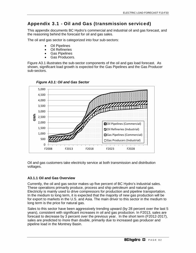
ELECTRIC LOAD FORECAST F13-F33
P A G E 8 2
Appendix 3.1 - Oil and Gas (transmission serviced) This appendix documents BC Hydro’s commercial and industrial oil and gas forecast, and the reasoning behind the forecast for oil and gas sales. The oil and gas sector is categorized into four sub-sectors:
• Oil Pipelines • Oil Refineries • Gas Pipelines • Gas Producers.
Figure A3.1 illustrates the sub-sector components of the oil and gas load forecast. As shown, significant load growth is expected for the Gas Pipelines and the Gas Producer sub-sectors.
Figure A3.1: Oil and Gas Sector
Oil and gas customers take electricity service at both transmission and distribution voltages.
A3.1.1 Oil and Gas Overview Currently, the oil and gas sector makes up five percent of BC Hydro’s industrial sales. These operations primarily produce, process and ship petroleum and natural gas. Electricity is mainly used to drive compressors for production and pipeline transportation. In the medium to long term, it is expected that the majority of new gas production will be for export to markets in the U.S. and Asia. The main driver to this sector in the medium to long term is the price for natural gas. Sales to this sector have been aggressively trending upward (by 28 percent over the last 5 years), consistent with significant increases in oil and gas production. In F2013, sales are forecast to decrease by 3 percent over the previous year. In the short term (F2012-2017), sales are predicted to more than double, primarily due to increased gas producer and pipeline load in the Montney Basin.
0
500
1,000
1,500
2,000
2,500
3,000
3,500
4,000
4,500
5,000
F2008 F2013 F2018 F2023 F2028
GW
h
Oil Pipelines (Commercial)
Oil Refineries (Industrial)
Gas Pipelines (Commercial)
Gas Producers (Industrial)

ELECTRIC LOAD FORECAST F13-F33
P A G E 8 3
In the medium term (F2017-F2022), oil and gas sales increase by about 60 percent, largely due to increased activity in oil and gas producer and pipeline load. For the latter 10 years of the forecast period, sales flatten in line with a levelling-off of gas production. Compared with the 2011 Forecast, the 2012 Forecast is lower in the short term but higher in the medium to long term. This is due to deferred gas production in the short term and increased gas production and Oil & Gas pipeline load in the medium and long term. Details are provided below. Note that gas producer load for the Horn River is treated as a separate scenario in the analysis for BC Hydro planning process. A3.1.2 Oil Pipelines Overview Sales to oil pipelines currently make up 17 percent of BC Hydro’s sales to the oil and gas sector. These customers operate pipelines which serve to transport crude oil and petroleum products. Electricity is primarily used in pumping stations and the power sales are correlated to the volume of liquids shipped. Since these customers are providing a service, as opposed to manufacturing a product, they are classified as commercial load. The main advantage enjoyed by B.C. pipeline operators is that the proximity to Asian markets is conducive to export. Oil Pipelines Outlook Over the last four years, sales have generally trended up as new pipeline capacity had been added to meet growing demand for exporting crude. In F2013, sales are forecast to increase materially compared to previous year, as operational constraints that were previously in place have been removed. For the first five years of the 2012 Forecast sales significantly increases as incremental pipeline capacity is expected to increase. From F2018 onward, oil pipelines sales are forecast to only marginally grow. Oil Pipelines Drivers and Risk Drivers:
• Addressing capacity constraints along the pipeline; • Demand for crude from California and Asia; • B.C. demand for crude, gasoline and jet fuel, and; • Economic conditions.
Risk Factors: • Environmental and social approvals for pipeline expansions and new
pipelines. • Construction risks and delays
A3.1.3 Oil Refineries Overview Sales to oil refineries make up 30 percent of the oil and gas sector. These customers extract, refine and store crude oil and are thus classified as industrial load. A small number of these customers (primarily located in the Lower Mainland) refine crude oil to produce gasoline and jet fuel. They also refine diesel by removing sulphur and provide liquid fuel storage. Sales in this sub-sector primarily depend on domestic demand from automobiles and air travel. In the future, oil refineries sales are expected to be relatively more dependent on export demand for crude oil and petroleum products. B.C. operators have a competitive

ELECTRIC LOAD FORECAST F13-F33
P A G E 8 4
advantage due to proximity to petroleum sources, dependability of shipping and receiving, and access to ports. Oil Refineries Outlook Over the last four years, sales have increased by 44 percent due to increases in oil production and refining activity. In F2013, sales are forecast to increase by 8 percent due to the expected recovery in gasoline, diesel and aircraft fuel sales. Over the entire forecast period, sales are expected to increase by 13 percent. Compared to the 2011 Forecast, oil refineries sales in the current forecast are relatively unchanged. Oil Refineries Drivers and Risk Drivers
• Demand for gasoline, diesel and jet fuel; • Oil and gasoline prices; and • Asian demand.
Risk Factors • Environmental concerns; • GHG regulations which might impact refineries; and • Local and global economic conditions.
A3.1.4 Gas Pipelines Overview Sales to this sub-sector compromises 10 percent of the total oil and gas sector sales. Pipeline companies use electricity for compressing gas for shipping and processing; this is not a manufacturing process, they are categorized as commercial customers. Gas Pipelines Outlook Over the last five years, the load in this sector has been relatively small and highly correlated to North American natural gas prices. Please see Appendix A3.2 for more information on northeastern B.C. gas production and electricity demand expectations.
Gas Pipeline Drivers and Risk Drivers:
• Potential for the conversion of coal-fired generation to less carbon-intensive natural gas-fired generation;
• Possible conversion of some of the Japanese nuclear fleet to gas-fired generation;
• Medium to long term expectations for gas and oil prices; • Carbon tax and fuel switching for GHG reduction purposes; BC Hydro would
tend to service more industry loads at higher carbon prices; and • Electrification of NE BC gas production.
Risk factors:
• Social concerns over the footprint of the extraction operations and the shipping and exporting of oil;
• Rate impacts to BC Hydro customers; and

ELECTRIC LOAD FORECAST F13-F33
P A G E 8 5
• The speed at which industry customers need electricity supply, and the ability of BC Hydro and the regulatory process to respond to these requests.
A3.1.5 Gas Producers Overview Sales to this sub-sector currently make up 45 percent of the oil and gas sales. The gas producers are located in northeastern B.C. and primarily use electricity to power their compressors. These customers are categorized as industrial because they produce and process either conventional gas or shale gas for sale. Although the production of conventional gas in B.C. is expected to progressively decline, shale gas production is forecast to grow substantially. BC Hydro anticipates it will be servicing a large portion of shale gas production (see Appendix 3.2).
Gas Producer Outlook Over the past five years, sector sales have risen by over 60 percent. In F2013, sales are forecast to remain relatively unchanged due to weak gas prices in the near term, which will dampen B.C. gas production. In the first five years of the 2012 Forecast, sales are projected to increase nearly six-fold; most of this growth attributable to shale gas development in the Montney Basin (refer to Appendix 3.2). During the F2018-23 period, sales growth is forecast to slow and flatten out as new drilling is expected to be directed at maintaining infrastructural efficiency. For the latter 10 years of the forecast, sales are expected to increase marginally with new drilling directed at maintaining gas flows at close to capacity to realize efficiencies. Compared to the 2011 Forecast, the current forecast for the Gas Producer sub-sector is lower in the short term but higher in the medium to long term. This is due to currently low natural gas prices in North America and uncertain financial markets have caused gas producers in the Montney gas basin to deferred drilling projects in the short term; however, in the medium to long term, greater than expected production activity is expected.
Gas Producer Drivers and Risk – See Appendix 3.2

ELECTRIC LOAD FORECAST F13-F33
P A G E 8 6
Appendix 3.2 - Shale Gas Producer Forecast – (Montney) Gas Producer Overview As indicated in Appendix A3.1, transmission and distribution customers serviced by BC Hydro for the production of shale gas are included in BC Hydro’s industrial customer sector. This appendix documents BC Hydro’s estimates of future load requirements for these shale gas producers. Shale gas refers to natural gas enclosed in a fine-grained sedimentary formation with low reservoir porosity and low permeability. Although such basins have been uneconomic in the past, new technological advancements such as horizontal drilling and multi-stage hydraulic fracturing have enhanced commercial production of shale gas. Sales for servicing shale gas production are expected to occur in northeast B.C. BC Hydro’s 2010 Load Forecast included expected sales from both the Horn River and Montney shale gas plays; the 2011 and 2012 Forecasts include sales from only the Montney play and treats potential Horn River sales as a separate scenario for analysis in BC Hydro’s long-term planning processes. For more detail on this point, refer to Chapter 9. Regarding the Montney, (in the vicinity of Dawson Creek, see Figure A3.1), sales are expected to increase substantially over the next 10 years, from current low levels, primarily due to regional shale gas development. The Montney Basin shales are believed to contain among the largest untapped reserves of unconventional gas in North America.
Figure A3.1. Map of Montney and Horn River Basins
BC Hydro is closely following a significant number of developments in the Montney area and potential liquid natural gas projects on BC’s North Coast. Below are recent public industry announcements which reflect continued global interest in the Montney Basin:
• In January 9, 2013, TransCanada Corp. announces plans to build a $5-billlion pipeline to transport gas to the North Coast from the North East to PETRONAS’ planned LNG plant near Prince Rupert.
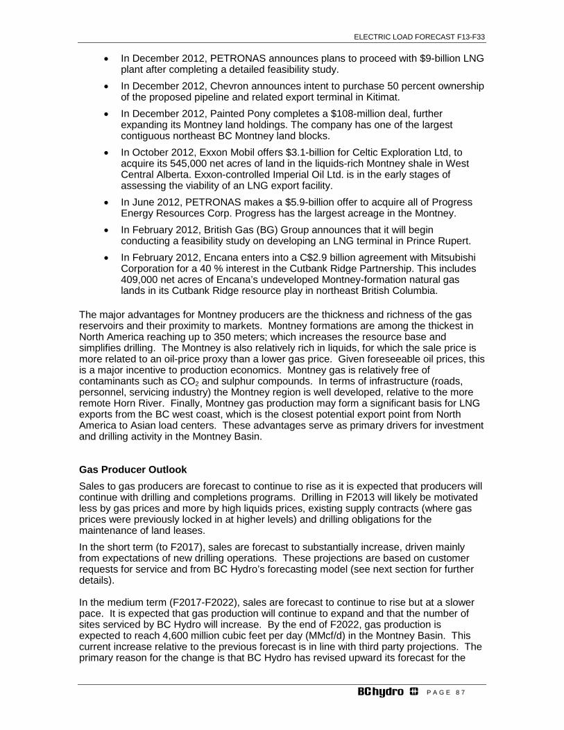
ELECTRIC LOAD FORECAST F13-F33
P A G E 8 7
• In December 2012, PETRONAS announces plans to proceed with $9-billion LNG plant after completing a detailed feasibility study.
• In December 2012, Chevron announces intent to purchase 50 percent ownership of the proposed pipeline and related export terminal in Kitimat.
• In December 2012, Painted Pony completes a $108-million deal, further expanding its Montney land holdings. The company has one of the largest contiguous northeast BC Montney land blocks.
• In October 2012, Exxon Mobil offers $3.1-billion for Celtic Exploration Ltd, to acquire its 545,000 net acres of land in the liquids-rich Montney shale in West Central Alberta. Exxon-controlled Imperial Oil Ltd. is in the early stages of assessing the viability of an LNG export facility.
• In June 2012, PETRONAS makes a $5.9-billion offer to acquire all of Progress Energy Resources Corp. Progress has the largest acreage in the Montney.
• In February 2012, British Gas (BG) Group announces that it will begin conducting a feasibility study on developing an LNG terminal in Prince Rupert.
• In February 2012, Encana enters into a C$2.9 billion agreement with Mitsubishi Corporation for a 40 % interest in the Cutbank Ridge Partnership. This includes 409,000 net acres of Encana’s undeveloped Montney-formation natural gas lands in its Cutbank Ridge resource play in northeast British Columbia.
The major advantages for Montney producers are the thickness and richness of the gas reservoirs and their proximity to markets. Montney formations are among the thickest in North America reaching up to 350 meters; which increases the resource base and simplifies drilling. The Montney is also relatively rich in liquids, for which the sale price is more related to an oil-price proxy than a lower gas price. Given foreseeable oil prices, this is a major incentive to production economics. Montney gas is relatively free of contaminants such as CO2 and sulphur compounds. In terms of infrastructure (roads, personnel, servicing industry) the Montney region is well developed, relative to the more remote Horn River. Finally, Montney gas production may form a significant basis for LNG exports from the BC west coast, which is the closest potential export point from North America to Asian load centers. These advantages serve as primary drivers for investment and drilling activity in the Montney Basin. Gas Producer Outlook Sales to gas producers are forecast to continue to rise as it is expected that producers will continue with drilling and completions programs. Drilling in F2013 will likely be motivated less by gas prices and more by high liquids prices, existing supply contracts (where gas prices were previously locked in at higher levels) and drilling obligations for the maintenance of land leases. In the short term (to F2017), sales are forecast to substantially increase, driven mainly from expectations of new drilling operations. These projections are based on customer requests for service and from BC Hydro’s forecasting model (see next section for further details). In the medium term (F2017-F2022), sales are forecast to continue to rise but at a slower pace. It is expected that gas production will continue to expand and that the number of sites serviced by BC Hydro will increase. By the end of F2022, gas production is expected to reach 4,600 million cubic feet per day (MMcf/d) in the Montney Basin. This current increase relative to the previous forecast is in line with third party projections. The primary reason for the change is that BC Hydro has revised upward its forecast for the
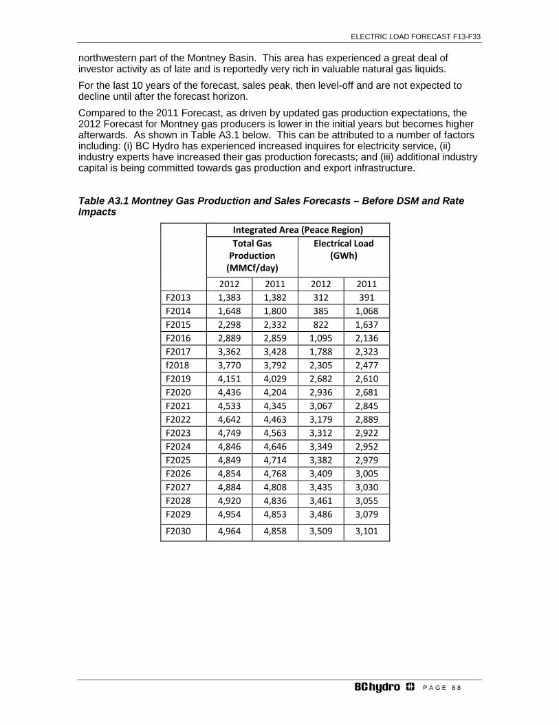
ELECTRIC LOAD FORECAST F13-F33
P A G E 8 8
northwestern part of the Montney Basin. This area has experienced a great deal of investor activity as of late and is reportedly very rich in valuable natural gas liquids. For the last 10 years of the forecast, sales peak, then level-off and are not expected to decline until after the forecast horizon. Compared to the 2011 Forecast, as driven by updated gas production expectations, the 2012 Forecast for Montney gas producers is lower in the initial years but becomes higher afterwards. As shown in Table A3.1 below. This can be attributed to a number of factors including: (i) BC Hydro has experienced increased inquires for electricity service, (ii) industry experts have increased their gas production forecasts; and (iii) additional industry capital is being committed towards gas production and export infrastructure.
Table A3.1 Montney Gas Production and Sales Forecasts – Before DSM and Rate Impacts
Integrated Area (Peace Region) Total Gas
Production (MMCf/day)
Electrical Load (GWh)
2012 2011 2012 2011 F2013 1,383 1,382 312 391 F2014 1,648 1,800 385 1,068 F2015 2,298 2,332 822 1,637 F2016 2,889 2,859 1,095 2,136 F2017 3,362 3,428 1,788 2,323 f2018 3,770 3,792 2,305 2,477 F2019 4,151 4,029 2,682 2,610 F2020 4,436 4,204 2,936 2,681 F2021 4,533 4,345 3,067 2,845 F2022 4,642 4,463 3,179 2,889 F2023 4,749 4,563 3,312 2,922 F2024 4,846 4,646 3,349 2,952 F2025 4,849 4,714 3,382 2,979 F2026 4,854 4,768 3,409 3,005 F2027 4,884 4,808 3,435 3,030 F2028 4,920 4,836 3,461 3,055 F2029 4,954 4,853 3,486 3,079
F2030 4,964 4,858 3,509 3,101

ELECTRIC LOAD FORECAST F13-F33
P A G E 8 9
Montney Shale Gas – Drivers and Risk Drivers
• Natural gas prices in North America – a high price stimulates sector demand because it makes it more profitable to produce shale gas;
• Price of oil – a high price elevates load demand. The Montney Basin is one of a limited number of North American gas plays that is rich in natural gas liquids; since liquids prices closely follow oil prices, a high oil price stimulates production in liquids-rich gas plays;
• Fracturing technology – evolving hydraulic fracturing technology produces proportionally greater benefits to the large rich shale gas plays such as the Montney.
Risk Factors • Greenhouse gas regulation – GHG emission reduction targets in B.C. and
the U.S.; • Regulation of formation fracturing operations – a number of provincial, state
and federal agencies are reviewing this, which may lead to constrained shale gas production;
• Other new N. American gas supply – which includes methyl hydrates, coal bed methane and other shale gas plays on the continent and associated gas in Alaska;
• New global gas supplies. Russia, China and Australia have shale gas potential. However, shale gas development in Asia is significantly behind that in N. America; and
• Montney development and operational costs – the Montney is relatively far from the major gas markets.
Shale Gas Forecast Methodology BC Hydro employs two approaches to develop the forecast, referred to as the bottom-up and top-down methodologies. The bottom-up forecast is based on customer-specific information and analysis and serves as BC Hydro’s official load forecast. The top-down forecast is a macro forecast that is used to guide and confirm the bottom-up forecast. Bottom-up Forecast The 2012 gas producer load forecast is generated using a bottom-up approach; it also includes an iterative exercise with the top-down forecast. The bottom-up forecast originates from a compilation of current and expected customer load requests. In arriving at an ‘expected’ or most likely net customer service requirement, each customer request is evaluated, shaped and discounted based on information from various sources internal and external to BC Hydro. External factors come from a number of areas such as industry, producer publications and the top-down forecast, as explained below. Top-down Forecast The top-down forecast uses macro information to arrive at the Montney load forecast. In doing so, it serves as a guide to check and improve the accuracy of the bottom-up forecast.
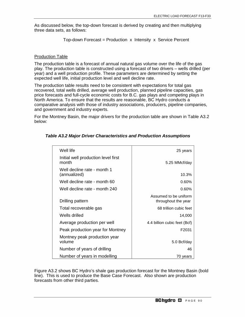
ELECTRIC LOAD FORECAST F13-F33
P A G E 9 0
As discussed below, the top-down forecast is derived by creating and then multiplying three data sets, as follows:
Top-down Forecast = Production x Intensity x Service Percent
Production Table The production table is a forecast of annual natural gas volume over the life of the gas play. The production table is constructed using a forecast of two drivers – wells drilled (per year) and a well production profile. These parameters are determined by setting the expected well life, initial production level and well decline rate. The production table results need to be consistent with expectations for total gas recovered, total wells drilled, average well production, planned pipeline capacities, gas price forecasts and full-cycle economic costs for B.C. gas plays and competing plays in North America. To ensure that the results are reasonable, BC Hydro conducts a comparative analysis with those of industry associations, producers, pipeline companies, and government and industry experts. For the Montney Basin, the major drivers for the production table are shown in Table A3.2 below:
Table A3.2 Major Driver Characteristics and Production Assumptions
Well life 25 years
Initial well production level first month 5.25 MMcf/day
Well decline rate - month 1 (annualized) 10.3%
Well decline rate - month 60 0.60%
Well decline rate - month 240 0.60%
Drilling pattern Assumed to be uniform
throughout the year
Total recoverable gas 68 trillion cubic feet
Wells drilled 14,000
Average production per well 4.4 billion cubic feet (Bcf)
Peak production year for Montney F2031
Montney peak production year volume 5.0 Bcf/day
Number of years of drilling 46
Number of years in modelling 70 years
Figure A3.2 shows BC Hydro’s shale gas production forecast for the Montney Basin (bold line). This is used to produce the Base Case Forecast. Also shown are production forecasts from other third parties.
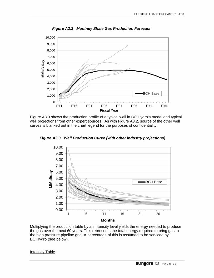
ELECTRIC LOAD FORECAST F13-F33
P A G E 9 1
Figure A3.2 Montney Shale Gas Production Forecast
Figure A3.3 shows the production profile of a typical well in BC Hydro’s model and typical well projections from other expert sources. As with Figure A3.2, source of the other well curves is blanked out in the chart legend for the purposes of confidentiality.
Figure A3.3 Well Production Curve (with other industry projections)
Multiplying the production table by an intensity level yields the energy needed to produce the gas over the next 60 years. This represents the total energy required to bring gas to the high pressure pipeline grid. A percentage of this is assumed to be serviced by BC Hydro (see below).
Intensity Table
0
1,000
2,000
3,000
4,000
5,000
6,000
7,000
8,000
9,000
10,000
F'11 F'16 F'21 F'26 F'31 F'36 F'41 F'46
MM
cf /
day
Fiscal Year
BCH Base
0.001.002.003.004.005.006.007.008.009.00
10.00
1 6 11 16 21 26
MM
cf/d
ay
Months
BCH Base

ELECTRIC LOAD FORECAST F13-F33
P A G E 9 2
The intensity factor is multiplied against gas production estimates to determine the total energy requirement needed to produce the gas. Intensity times production equals total energy needed, as shown in the equation below: Intensity (MW/MMcf/day) x Production (MMcf/day) = Power Requirement (MW)
where: MW is megawatts of power consumption and MMcf/day is million cubic feet of gas per day
BC Hydro’s intensity rate is a compilation of two approaches: (a) determining the energy requirements of the major processes within a typical plant, and (b) conducting an industry survey. BC Hydro’s calculation factors for estimating the typical plant requirement are detailed below:
Compression 0.105 MW/MMcf/d + Processing 0.025 MW/MMcf/d + Additional Compression 0.001 to 0.01 MW/MMcf/d = Total 0.131 to 0.140 MW/MMcf/d
As shown above, the total intensity rate range is 0.131 to 0.140 MW/MMcf/d. This is comparable to industry information indicating a range of 0.08 to 0.14 MW/MMcf/day, with a number of estimates clustered around a value of 0.120.
The compression intensity of 0.105 MW/MMcf represents the energy needed to move the gas from the wellhead, through the field gathering system and into a centralized processing facility (where electricity is also used in the processing process, (which includes the removal of gas liquids) and then eventually to the high-pressure, downstream pipeline. This calculation assumes:
• Well-head pressures of 140 to 240 Psi • Mainline pipe pressure of 900 to 1,440 Psi • 2 or 3 stages of compression.
The processing intensity of 0.025 MW/MMcf/d is for ancillary electric loads for removing water, acid gases and liquids. In the Montney, gas can be processed at the processing facility since gathering pressures are low and the gas generally is only slightly sour. This estimate assumes:
• Only a small portion of gas in the Montney is sour (in the regions closest to the Alberta border), per industry sources; and
• The water content of the gas is low and much of the gas meets pipeline specifications of about four pounds of water per MMcf of gas.
The additional compression intensity of 0.001 to 0.01 MW/MMcf/d is BC Hydro’s estimate for additional load that is expected to be required to move gas from the processing facility to the downstream pipeline. As the Montney play develops, additional pipeline compression is expected to be required to move gas downstream. Other assumptions:
• Hydraulic fracturing operations would not require service from BC Hydro; these operations are of a short duration and generally in remote locations;
• Water recycling loads would not be material; • Downstream pipeline loads would not be served by BC Hydro.

ELECTRIC LOAD FORECAST F13-F33
P A G E 9 3
Service Percent Table The service percent is the proportion of total energy to be provided by BC Hydro’s electricity service. A number of factors have been considered by BC Hydro in arriving at this figure – namely, evolving trends for the areas, engineering calculations and economic analysis, discussion with BC Hydro staff who work directly with the new customers and industry surveys conducted by BC Hydro. For the Montney Basin, the forecast is divided into five areas with the following service percentages:
• Dawson Creek: 40% ramping up to 85% over the forecast horizon • Groundbirch: 30% ramping up to 95% • Chetwynd: 40% ramping up to 85% • Fox/Fort St. John: 5% ramping up to 70% • G.M. Shrum: 15% ramping up to 25%.

ELECTRIC LOAD FORECAST F13-F33
P A G E 9 4
Appendix 3.3 – LNG Load Outlook
Demand for natural gas is growing in Asia and Europe, primarily for electricity generation and heating purposes, as well as in transportation. China and Japan are both pursuing new supply options – China to fuel its massive modernization and Japan to diversify its fuel supply. With demand growing quickly, gas prices in Asia are considerably higher than they are in North America. This creates the opportunity for natural gas exports to these markets in the form of LNG. To date, several LNG proponents have approached BC Hydro and/or the B.C. Government with respect to LNG projects for the B.C. north coast. Canadian producers are increasingly looking to take advantage of this price differential, with a number of LNG export projects being proposed. LNG is a very capital intensive undertaking; these operations typically run at very high load factors, with minimal downtime, and little seasonal or intra-day load variations. Over the past couple of years, BC Hydro and government have been closely working with LNG proponents on options for meeting all or some of the energy needs of LNG plants with power from the BC Hydro system. LNG-related electricity demand falls in to two general categories: compression and non-compression. The compression work energy is about 85% of the total plant’s energy needs. The remaining (non-compression) energy requirement is from plant pumps, motors, other equipment, heating and lighting. Compression energy is typically supplied with direct-drive natural gas turbines, although this can also be accomplished with electric drives. Nevertheless, LNG non-compression demand is still significant, and could be one of BC Hydro’s biggest system loads. Potential non-compression LNG demand could be between about 800 GWh/year to about 6,600 GWh/year of additional energy demand, corresponding to about 100 MW to 800 MW of additional peak demand. A range of potential LNG loads are considered as scenarios in BC Hydro’s planning processes. The 2012 Reference Load Forecast presented in this document does not include any specific LNG demand beyond very small allocations associated with on-site construction.

ELECTRIC LOAD FORECAST F13-F33
P A G E 9 5
Appendix 4 - Electric Vehicles (EVs) Overview In the past two years automobile manufactures have launched several models of electric vehicles (EVs) in North America while announcing plans for mass production of EVs in the near future. However, the market is still new and uncertainties remain around the timing and extent of large-scale adoption of EVs. The operating cost and environmental advantages of EVs make them attractive alternatives to conventional gasoline vehicles. On the other hand, the generally higher purchase price of EVs and lower gasoline prices may dampen the market share growth of EVs. EVs have a large fuel cost advantage over gasoline vehicles, offering drivers lower ongoing operating costs. The low price of electricity in BC compared to other North American jurisdictions further magnifies the operating cost advantage of EVs. Large-scale adoption of EVs may help lower greenhouse gas emissions and related environmental costs. Some of the key barriers that need to be overcome before EVs gain a significant market share include: higher costs, limited driving range of EVs, and overall consumer acceptance as alternative to gas vehicles. The purchase price of EVs remains significantly higher than the price of comparable gasoline vehicles, in part due to the high cost of batteries. Despite major research and development investments in battery technology by the private sector and governments, battery prices remain high and some battery manufacturers have faced financial difficulties. The limited range of all-electric vehicles is an obstacle for drivers who drive long distances; this may be a challenge for both urban and rural drivers in various parts of the province. Even drivers who seldom travel distances longer than the current range of EVs may forego this option due to “range anxiety” – the perceived threat of being stranded. While plug-in hybrid electric vehicles (PHEVs) offer extended range and therefore reduce range anxiety, their higher costs compared to pure EVs limits their attractiveness to potential buyers. Availability of public charging infrastructure and consumer education are ways to reduce range anxiety. EV Impacts on Energy Demand The load forecast of EVs consists of a reference case and a high case scenario. A forecast of the number of EVs and annual energy consumption of EVs is created. The forecast is produced using a model that takes into account many variables including driving-age population and vehicle growth, gasoline and electricity price forecasts, and efficiencies for both electric and conventional vehicles. The EV reference case forecast includes the following main assumptions:
• A constant energy efficiency of 30 miles per gallon for gasoline vehicles and 0.20 KWh per km for EVs.
• Existing government subsidies are taken into account, but no new policies or initiatives are assumed.
• The supply and demand for EVs is initially constrained because the EV fleet is currently very small and the rate of development depends upon several factors. These factors include: consumers’ tastes and acceptance of EVs, and time needed for manufacturing capacity to expand in areas of battery production, retrofitting current factories or creating new facilities dedicated to EV manufacturing.
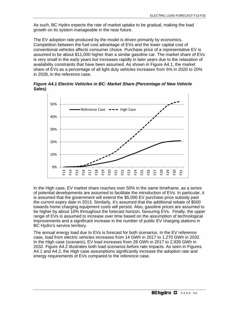
ELECTRIC LOAD FORECAST F13-F33
P A G E 9 6
As such, BC Hydro expects the rate of market uptake to be gradual, making the load growth on its system manageable in the near future. The EV adoption rate produced by the model is driven primarily by economics. Competition between the fuel cost advantage of EVs and the lower capital cost of conventional vehicles affects consumer choice. Purchase price of a representative EV is assumed to be about $11,000 higher than a similar gasoline car. The market share of EVs is very small in the early years but increases rapidly in later years due to the relaxation of availability constraints that have been assumed. As shown in Figure A4.1, the market share of EVs as a percentage of all light duty vehicles increases from 5% in 2020 to 20% in 2028, in the reference case.
Figure A4.1 Electric Vehicles in BC: Market Share (Percentage of New Vehicle Sales)
In the High case, EV market share reaches over 50% in the same timeframe, as a series of potential developments are assumed to facilitate the introduction of EVs. In particular, it is assumed that the government will extend the $5,000 EV purchase price subsidy past the current expiry date in 2013. Similarly, it’s assumed that the additional rebate of $500 towards home charging equipment costs will persist. Also, gasoline prices are assumed to be higher by about 10% throughout the forecast horizon, favouring EVs. Finally, the upper range of EVs is assumed to increase over time based on the assumption of technological improvements and a significant increase in the number of public EV charging stations in BC Hydro’s service territory. The annual energy load due to EVs is forecast for both scenarios. In the EV reference case, load from electric vehicles increases from 14 GWh in 2017 to 1,270 GWh in 2032. In the High case (scenario), EV load increases from 28 GWh in 2017 to 2,939 GWh in 2032. Figure A4.2 illustrates both load scenarios before rate impacts. As seen in Figures A4.1 and A4.2, the High case assumptions significantly increase the adoption rate and energy requirements of EVs compared to the reference case.
0%
10%
20%
30%
40%
50%
F13
F14
F15
F16
F17
F18
F19
F20
F21
F22
F23
F24
F25
F26
F27
F28
F29
F30
F31
Reference Case High Case

ELECTRIC LOAD FORECAST F13-F33
P A G E 9 7
Figure A4.2 EV Load Forecast
Table A4.1 at the end of this appendix shows the residential EV load, commercial EV load and the total EV load included in the 2012 reference load forecast. EV Impacts on Peak Demand BC Hydro developed an EV peak model to study the impact of EVs on BC Hydro’s system peak. The peak EV model was updated in the 2012 Forecast with consistent inputs from the EV energy model. The EV peak model is a simulation model that has several inputs including: (i) number of EVs per year; (ii) daily distance travelled; (iii) EV efficiency in kWh per km; (iv) power of the charging equipment in kW; and (v) a charging time profile. These inputs combine in the simulation model to determine an EV daily peak shape which is used to estimate the EV impact on BC Hydro system coincident peak demand. The model does not account for specific peak shifting behaviour. This means the model produces the impact on the peak demand without any constraints to shift EV load impact away from the system peak hours. It is possible that when EVs become available in large numbers, incentives or policies may be used to mitigate EV contribution to the system peak load. Overall, the impact of EVs on BC Hydro peak in the reference case is approximately 4 MW in F2017 and 459 MW in F2032. Figure A4.3 below and table A4.1 show the EV impact on BC Hydro’s total distribution system coincident peak before DSM and rate impacts and before system transmission losses.
0
500
1000
1500
2000
2500
3000
F13
F14
F15
F16
F17
F18
F19
F20
F21
F22
F23
F24
F25
F26
F27
F28
F29
F30
F31
F32
GW
h Reference Case High Case
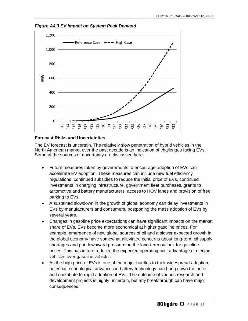
ELECTRIC LOAD FORECAST F13-F33
P A G E 9 8
Figure A4.3 EV Impact on System Peak Demand
Forecast Risks and Uncertainties The EV forecast is uncertain. The relatively slow penetration of hybrid vehicles in the North American market over the past decade is an indication of challenges facing EVs. Some of the sources of uncertainty are discussed here:
• Future measures taken by governments to encourage adoption of EVs can accelerate EV adoption. These measures can include new fuel efficiency regulations, continued subsidies to reduce the initial price of EVs, continued investments in charging infrastructure, government fleet purchases, grants to automotive and battery manufacturers, access to HOV lanes and provision of free parking to EVs.
• A sustained slowdown in the growth of global economy can delay investments in EVs by manufacturers and consumers, postponing the mass adoption of EVs by several years.
• Changes in gasoline price expectations can have significant impacts on the market share of EVs. EVs become more economical at higher gasoline prices. For example, emergence of new global sources of oil and a slower expected growth in the global economy have somewhat alleviated concerns about long-term oil supply shortages and put downward pressure on the long-term outlook for gasoline prices. This has in turn reduced the expected operating cost advantage of electric vehicles over gasoline vehicles.
• As the high price of EVs is one of the major hurdles to their widespread adoption, potential technological advances in battery technology can bring down the price and contribute to rapid adoption of EVs. The outcome of various research and development projects is highly uncertain, but any breakthrough can have major consequences.
0
200
400
600
800
1,000
1,200
F13
F14
F15
F16
F17
F18
F19
F20
F21
F22
F23
F24
F25
F26
F27
F28
F29
F30
F31
F32
MW
Reference Case High Case

ELECTRIC LOAD FORECAST F13-F33
P A G E 9 9
• Similarly, increased competition from alternative technologies can reduce the appeal of EVs. For example, gasoline vehicles continue to improve in efficiency as a result of lighter components, turbochargers, regenerative braking and energy recovery technologies and other technological advances. Clean diesel, natural gas, and hybrid vehicles also compete with EVs for market share
• Changes in driving habits of drivers and increased use of public transit and other alternative transportation can also impact the market share of EVs. Statistics show a general trend of decreasing vehicle kilometers driven. Drivers who commute shorter distances or regularly take public transit will not benefit as much from the operating cost advantage of EVs and may favour conventional vehicles.
• In recent years consumers have been keeping their cars longer and delaying new car purchases. If this trend continues, the replacement of existing fleet of predominantly gasoline vehicles is expected to occur at a slower pace.
Comparison to 2011 Forecast Figures A4.4 and A4.5 compare the F2011 and F2012 EV reference forecasts. The energy consumption by EVs is 188 GWh (54%) lower by F2022 and almost 1000 GWh (46%) lower by F2032. Factors contributing to a lower forecast include:
• The new forecast considers the downward trend in distances travelled by BC drivers
• Conventional vehicles are continuing to show improvements in efficiency • New vehicle purchase statistics have declined, reducing expectations of new
vehicle sales and expected rate of replacement of the existing fleet of vehicles • Technological advances and new sources of oil have led to lower gasoline price
forecasts
The EV peak model was not updated in 2011. The peak impact of EVs beyond the first 10-year period of the load forecast was assumed in 2011 to follow the energy load growth rates that are used to develop the distribution peak forecast over this period. The growth rates in the total of EV energy sales, residential sales and small commercial and industrial sales were used to grow the overall peak demand rather than adding the EV model peak impact to the overall System peak forecast. In 2012, the EV peak model was updated as described earlier in this section. Although the EV energy forecast is lower in 2012 as a result of lower number of EVs and distance travelled, the EV peak values are relatively close between 2011 and 2012. This is mainly due to the fact that EV peak values in 2012 are generated by the EV peak model instead of following the overall distribution energy load growth.
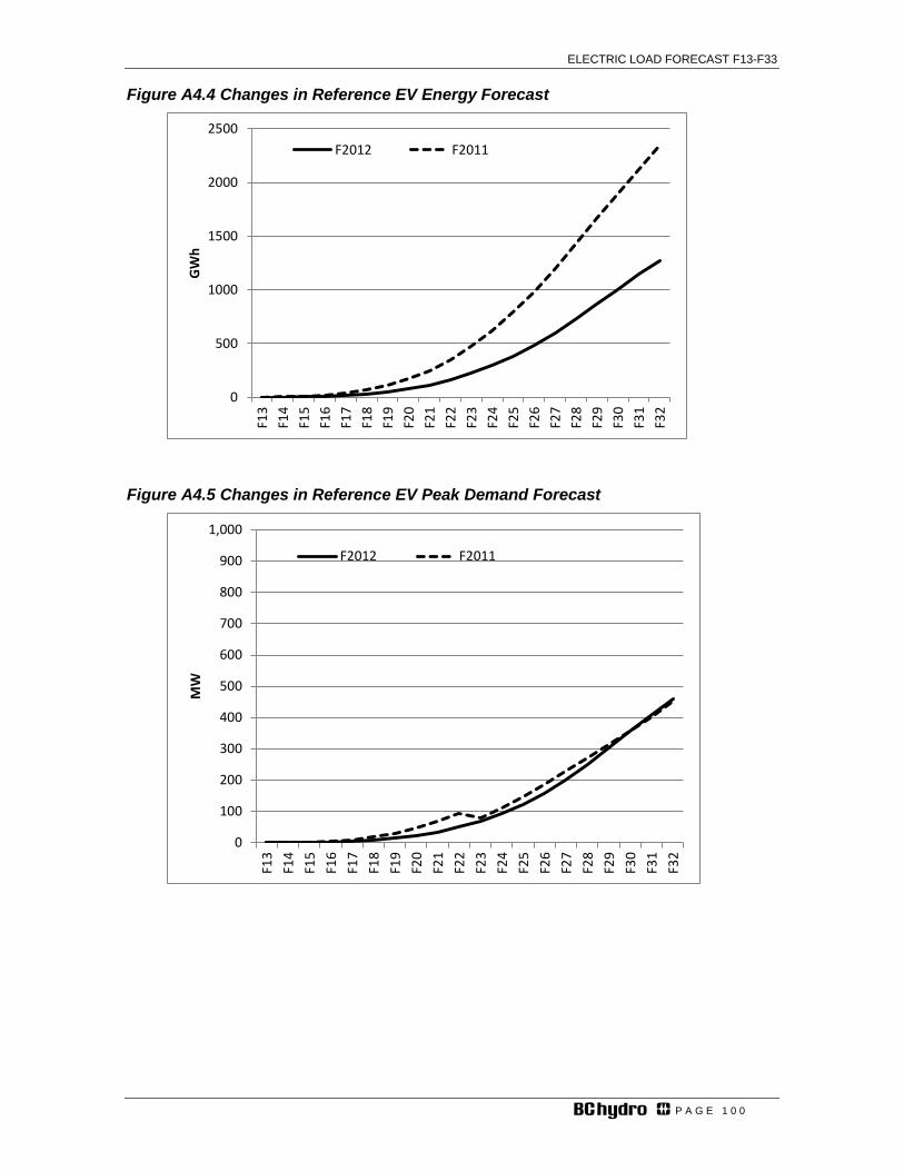
ELECTRIC LOAD FORECAST F13-F33
P A G E 1 0 0
Figure A4.4 Changes in Reference EV Energy Forecast
Figure A4.5 Changes in Reference EV Peak Demand Forecast
0
500
1000
1500
2000
2500
F13
F14
F15
F16
F17
F18
F19
F20
F21
F22
F23
F24
F25
F26
F27
F28
F29
F30
F31
F32
GW
h
F2012 F2011
0
100
200
300
400
500
600
700
800
900
1,000
F13
F14
F15
F16
F17
F18
F19
F20
F21
F22
F23
F24
F25
F26
F27
F28
F29
F30
F31
F32
MW
F2012 F2011
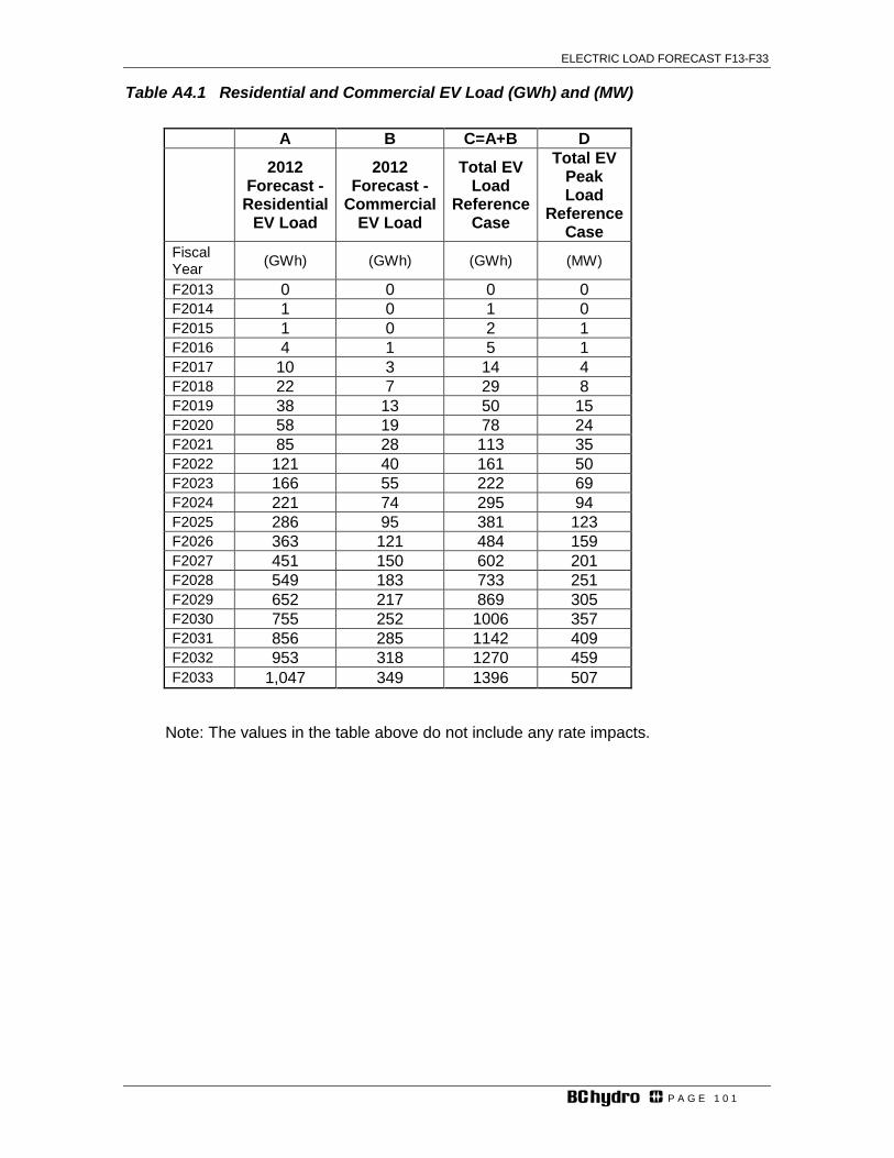
ELECTRIC LOAD FORECAST F13-F33
P A G E 1 0 1
Table A4.1 Residential and Commercial EV Load (GWh) and (MW)
A B C=A+B D
2012 Forecast - Residential
EV Load
2012 Forecast -
Commercial EV Load
Total EV Load
Reference Case
Total EV Peak Load
Reference Case
Fiscal Year (GWh) (GWh) (GWh) (MW)
F2013 0 0 0 0 F2014 1 0 1 0 F2015 1 0 2 1 F2016 4 1 5 1 F2017 10 3 14 4 F2018 22 7 29 8 F2019 38 13 50 15 F2020 58 19 78 24 F2021 85 28 113 35 F2022 121 40 161 50 F2023 166 55 222 69 F2024 221 74 295 94 F2025 286 95 381 123 F2026 363 121 484 159 F2027 451 150 602 201 F2028 549 183 733 251 F2029 652 217 869 305 F2030 755 252 1006 357 F2031 856 285 1142 409 F2032 953 318 1270 459 F2033 1,047 349 1396 507
Note: The values in the table above do not include any rate impacts.

ELECTRIC LOAD FORECAST F13-F33
P A G E 1 0 2
Appendix 5 - Codes and Standards Overlap with DSM Codes and standards are minimum end-use efficiency requirements that come into effect in a jurisdiction, and that are enabled by legislation or by regulation of manufacturers. U.S based codes and standards are reflected in the average stock efficiency forecast of residential and commercial end uses of electricity produced by the U.S. Department of Energy’s Energy Information Administration (EIA). This EIA efficiency forecast is one of the main drivers of the residential and small commercial end-use models that are used to produce the BC Hydro load forecast before incremental Demand Side Management (DSM) savings. BC Hydro’s DSM plan also considers savings that can be achieved from B.C. and Canadian Federal codes and standards that target similar end uses as those represented in the EIA efficiency forecast data. As such, there is a potential for inconsistency in codes and standards baseline assumptions between the before DSM Forecast and the DSM plan. Areas of Overlap between EIA and DSM Plan Codes and Standards The EIA assumes that no new legislation or regulations fostering efficiency improvements beyond those currently embodied in law or government programs will take place over the forecast horizon. As such, the end-use efficiency levels assumed in the EIA forecast only consider the targeted efficiency level from the mostly recently passed legislation or regulations. These efficiency level assumptions are documented by the EIA12. BC Hydro reviewed the EIA baseline codes and standards efficiency assumptions and compared it to the codes and standards baseline efficiency assumptions as of December 2011. Using this information, BC Hydro was able to determine where there were overlaps in assumptions between the before DSM and rate impacts forecast and the savings from codes and standards. The areas are shown as follows:
Areas of Overlap between EIA Codes and Standards and BC Hydro DSM Plan13 Residential Sector Lighting, ceiling fans, dishwashers, stand-
by power, set top boxes, TVs, freezers, refrigerators and external power supply
Commercial Sector Lighting, large clothes washers, traffic lights, large refrigerators, air conditioning, packaged terminal air conditioning, dry transformers, and building code.
Estimates of Overlap between EIA Codes and Standards and the DSM Savings from Codes and Standards The method used in the 2012 Forecast to estimate the impact of codes and standards double counting was to rely upon on the estimated codes and standard savings included in the BC Hydro DSM plan14. For lighting codes and standards double counting, a process
12 Appendix A of the EIA Annual Energy Outlook 2009 documents titled “Handling of Federal and Selected State Legislation and Regulation in the Annual Energy Outlook”. In addition information from EIA 2011 Annual Energy Outlook and website www.appliance-standards.org was used to develop estimates of the overlap. 13 Note that in all of the end uses listed, the EIA provides an efficiency forecast for lighting separately. The other end uses listed above are reflected in the “other” category and the EIA provides an efficiency forecast for other category as a total group. 14 The codes and standards savings forecast included in BC Hydro’s DSM plan contained in the F12-F14 Revenue Requirement Application Evidentiary Update was used to inform estimates of the overlap in codes and standards.

ELECTRIC LOAD FORECAST F13-F33
P A G E 1 0 3
of freezing the input efficiency levels to the 2007 lighting efficiency forecast was used. This method for lighting was chosen to provide consistency with previous forecasts that had already identified a double counting issue with lighting codes and standards. BC Hydro applied 50 percent of the DSM savings estimates of the various codes and standards which overlapped with the EIA. The main reasons for discounting half of the DSM estimates were:
• There is the potential for some error in the double counting impact estimating process because there is uncertainty as to compliance levels for codes and standards.
• At the time the load forecast was developed BC Hydro was exploring several future DSM options. As such the overlap associated with the double counted end-uses might vary pending which DSM option would be used for planning purposes.
Table A5.1 and Table A5.2 below show the estimates of the overlap between the residential and commercial sector energy forecasts for the overlap areas. Table A5.3 below shows the BC Hydro’s distribution peak forecast with an estimate of the overlap between codes and standards over the long-term.
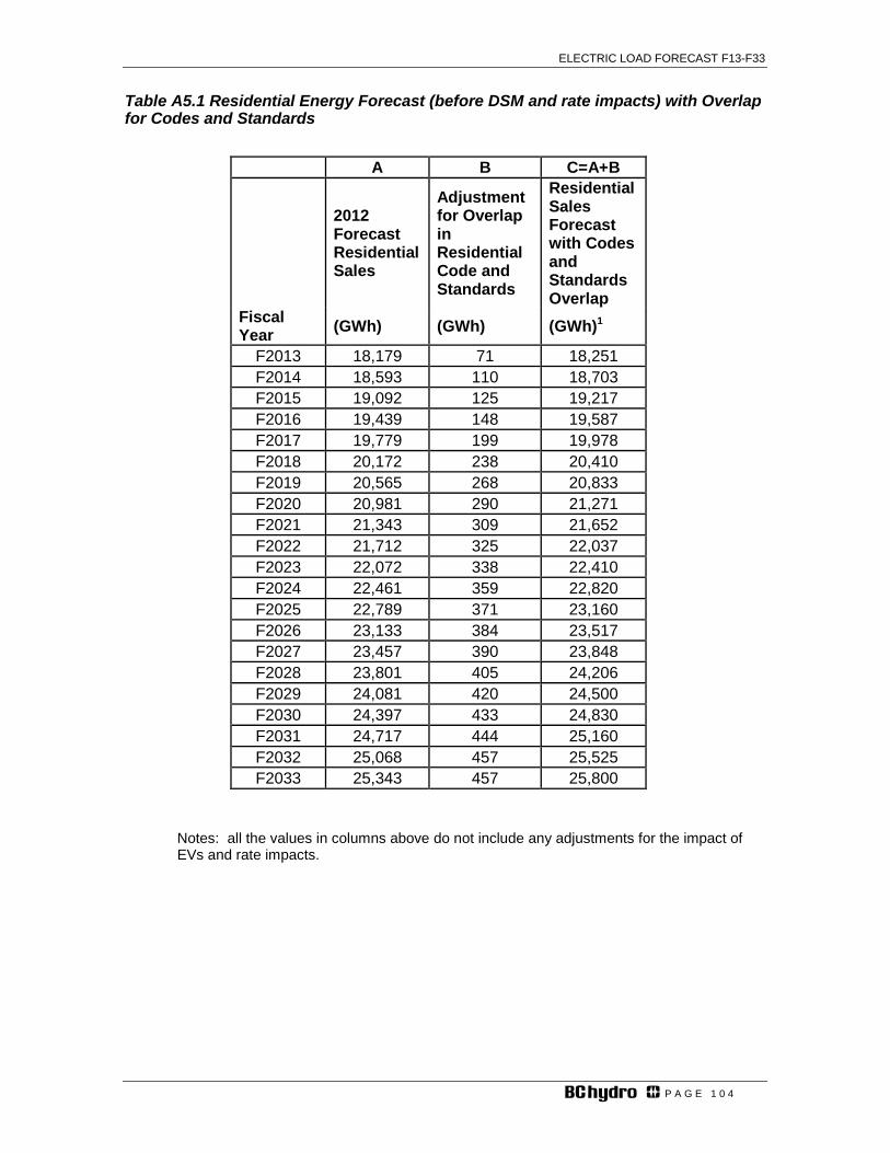
ELECTRIC LOAD FORECAST F13-F33
P A G E 1 0 4
Table A5.1 Residential Energy Forecast (before DSM and rate impacts) with Overlap for Codes and Standards
A B C=A+B
2012 Forecast Residential Sales
Adjustment for Overlap in Residential Code and Standards
Residential Sales Forecast with Codes and Standards Overlap
Fiscal Year (GWh) (GWh) (GWh)1
F2013 18,179 71 18,251 F2014 18,593 110 18,703 F2015 19,092 125 19,217 F2016 19,439 148 19,587 F2017 19,779 199 19,978 F2018 20,172 238 20,410 F2019 20,565 268 20,833 F2020 20,981 290 21,271 F2021 21,343 309 21,652 F2022 21,712 325 22,037 F2023 22,072 338 22,410 F2024 22,461 359 22,820 F2025 22,789 371 23,160 F2026 23,133 384 23,517 F2027 23,457 390 23,848 F2028 23,801 405 24,206 F2029 24,081 420 24,500 F2030 24,397 433 24,830 F2031 24,717 444 25,160 F2032 25,068 457 25,525 F2033 25,343 457 25,800
Notes: all the values in columns above do not include any adjustments for the impact of EVs and rate impacts.
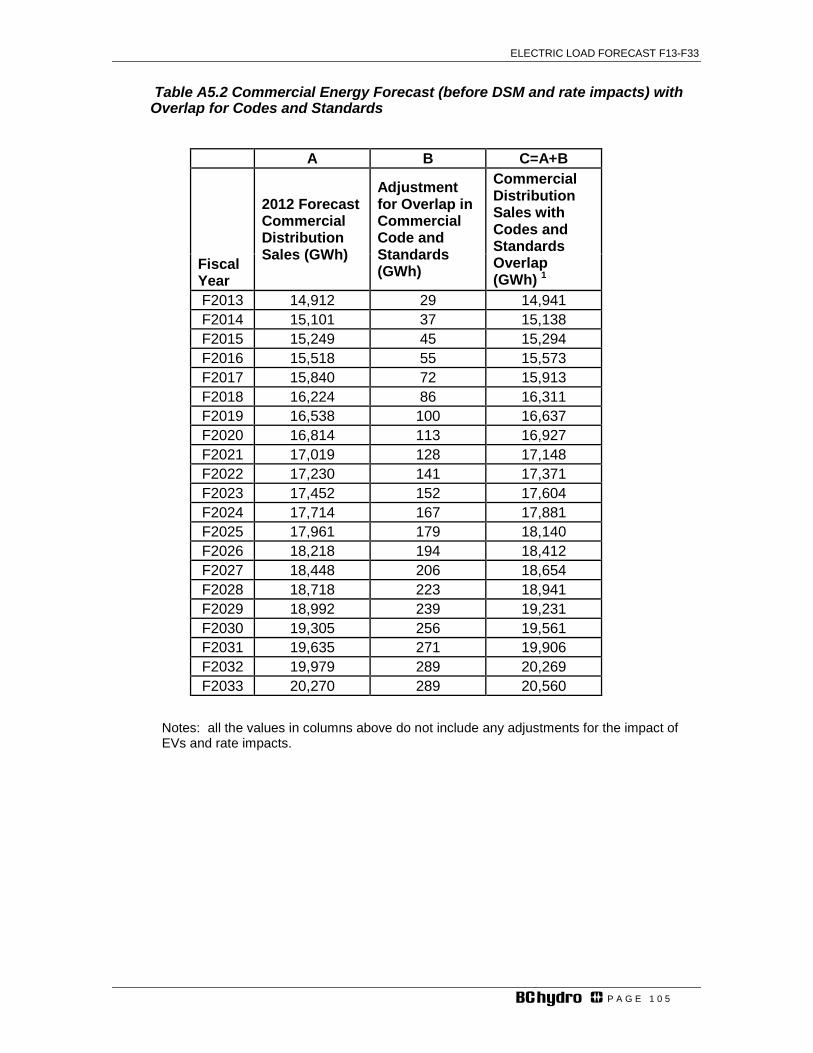
ELECTRIC LOAD FORECAST F13-F33
P A G E 1 0 5
Table A5.2 Commercial Energy Forecast (before DSM and rate impacts) with Overlap for Codes and Standards
A B C=A+B
2012 Forecast Commercial Distribution Sales (GWh)
Adjustment for Overlap in Commercial Code and Standards (GWh)
Commercial Distribution Sales with Codes and Standards Overlap (GWh) 1
Fiscal Year F2013 14,912 29 14,941 F2014 15,101 37 15,138 F2015 15,249 45 15,294 F2016 15,518 55 15,573 F2017 15,840 72 15,913 F2018 16,224 86 16,311 F2019 16,538 100 16,637 F2020 16,814 113 16,927 F2021 17,019 128 17,148 F2022 17,230 141 17,371 F2023 17,452 152 17,604 F2024 17,714 167 17,881 F2025 17,961 179 18,140 F2026 18,218 194 18,412 F2027 18,448 206 18,654 F2028 18,718 223 18,941 F2029 18,992 239 19,231 F2030 19,305 256 19,561 F2031 19,635 271 19,906 F2032 19,979 289 20,269 F2033 20,270 289 20,560
Notes: all the values in columns above do not include any adjustments for the impact of EVs and rate impacts.
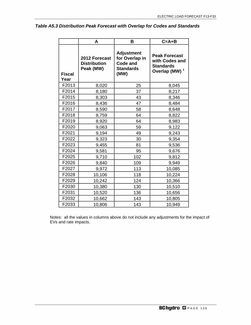
ELECTRIC LOAD FORECAST F13-F33
P A G E 1 0 6
Table A5.3 Distribution Peak Forecast with Overlap for Codes and Standards
A B C=A+B
2012 Forecast Distribution Peak (MW)
Adjustment for Overlap in Code and Standards (MW)
Peak Forecast with Codes and Standards Overlap (MW) 1 Fiscal
Year F2013 8,020 25 8,045 F2014 8,180 37 8,217 F2015 8,303 43 8,346 F2016 8,436 47 8,484 F2017 8,590 58 8,648 F2018 8,759 64 8,822 F2019 8,920 64 8,983 F2020 9,063 59 9,122 F2021 9,194 49 9,243 F2022 9,323 30 9,354 F2023 9,455 81 9,536 F2024 9,581 95 9,676 F2025 9,710 102 9,812 F2026 9,840 109 9,949 F2027 9,972 113 10,085 F2028 10,106 118 10,224 F2029 10,242 124 10,366 F2030 10,380 130 10,510 F2031 10,520 136 10,656 F2032 10,662 143 10,805 F2033 10,806 143 10,949
Notes: all the values in columns above do not include any adjustments for the impact of EVs and rate impacts.

ELECTRIC LOAD FORECAST F13-F33
P A G E 1 0 7
Appendix 6 - Forecast Tables Table A6.1 shows the Regional coincident peak (MW) forecast for distribution before DSM with rate impacts Table A6.2 shows the Regional coincident peak (MW) forecast for transmission before DSM with rate impacts Table A6.3 shows the Domestic and Regional peak forecast before DSM with rate impacts Table A6.4 summarizes BC Hydro’s 2012 Reference Load Forecast before DSM with rate impacts

ELECTRIC LOAD FORECAST F13-F33
P A G E 1 0 8
Table A6.1 Regional Coincident Distribution Peaks Before DSM with Rate Impacts (MW)
Fiscal Year
Coincident Peak (MW)
Lower Mainland
Vancouver Island
South Interior
Northern Region
Actual F2012 4,505 1,801 1,024 735
Weather-Normalized Actual F2012 4,554 1,862 1,035 737
Forecast (Weather-Normalized) F2013 4,664 1,905 1,051 765 F2014 4,777 1,937 1,070 782 F2015 4,837 1,948 1,084 799 F2016 4,914 1,963 1,094 813 F2017 5,008 1,980 1,106 839 F2018 5,118 2,001 1,120 862 F2019 5,224 2,021 1,133 888 F2020 5,333 2,039 1,145 907 F2021 5,430 2,057 1,158 922 F2022 5,527 2,074 1,168 935 F2023 5,661 2,103 1,187 959 F2024 5,779 2,129 1,201 968 F2025 5,899 2,155 1,216 976 F2026 6,025 2,182 1,231 984 F2027 6,156 2,210 1,247 992 F2028 6,296 2,240 1,264 1,001 F2029 6,441 2,272 1,282 1,010 F2030 6,588 2,303 1,300 1,019 F2031 6,736 2,335 1,317 1,029 F2032 6,884 2,366 1,335 1,038 F2033 7,030 2,396 1,352 1,046
5 years: F2012 to F2017 1.9% 1.2% 1.3% 2.6% 11 years: F2012 to F2023 2.0% 1.1% 1.3% 2.4% 21 years: F2012 to F2033 2.1% 1.2% 1.3% 1.7%
Notes:
1. Growth rates based on weather normalized actual peak. 2. Vancouver Island peak values include Gulf Island’s peak requirements.

ELECTRIC LOAD FORECAST F13-F33
P A G E 1 0 9
Table A6.2 Regional Coincident Transmission Peaks Before DSM with Rate Impacts (MW)
Fiscal Year
Coincident Peak (MW)
Lower Mainland
Vancouver Island
South Interior
Northern Region
Actual F2012 326 249 289 605
Forecast F2013 424 238 312 590 F2014 424 241 324 630 F2015 430 238 330 723 F2016 432 237 342 816 F2017 437 237 343 883 F2018 445 234 366 966 F2019 448 234 364 1,051 F2020 451 234 365 1,093 F2021 453 234 366 1,112 F2022 453 234 365 1,099 F2023 455 234 365 1,087 F2024 463 234 359 1,086 F2025 465 228 360 1,077 F2026 469 228 323 1,079 F2027 470 228 268 1,115 F2028 472 228 249 1,136 F2029 474 229 250 1,140 F2030 476 229 251 1,147 F2031 479 229 253 1,151 F2032 481 228 256 1,151 F2033 482 228 261 1,149
5 years: F2012 to F2017 6.0% -1.0% 3.5% 7.8% 11 years: F2012 to F2023 3.1% -0.6% 2.2% 5.5% 21 years: F2012 to F2033 1.9% -0.4% -0.5% 3.1%
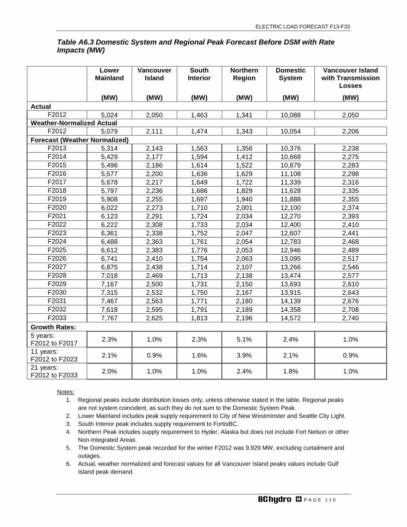
ELECTRIC LOAD FORECAST F13-F33
P A G E 1 1 0
Table A6.3 Domestic System and Regional Peak Forecast Before DSM with Rate Impacts (MW)
Lower Mainland
(MW)
Vancouver Island
(MW)
South Interior
(MW)
Northern Region
(MW)
Domestic System
(MW)
Vancouver Island with Transmission
Losses
(MW) Actual
F2012 5,024 2,050 1,463 1,341 10,088 2,050 Weather-Normalized Actual
F2012 5,079 2,111 1,474 1,343 10,054 2,206 Forecast (Weather Normalized)
F2013 5,314 2,143 1,563 1,356 10,376 2,238 F2014 5,429 2,177 1,594 1,412 10,668 2,275 F2015 5,496 2,186 1,614 1,522 10,879 2,283 F2016 5,577 2,200 1,636 1,629 11,108 2,298 F2017 5,678 2,217 1,649 1,722 11,339 2,316 F2018 5,797 2,236 1,686 1,829 11,628 2,335 F2019 5,908 2,255 1,697 1,940 11,888 2,355 F2020 6,022 2,273 1,710 2,001 12,100 2,374 F2021 6,123 2,291 1,724 2,034 12,270 2,393 F2022 6,222 2,308 1,733 2,034 12,400 2,410 F2023 6,361 2,338 1,752 2,047 12,607 2,441 F2024 6,488 2,363 1,761 2,054 12,783 2,468 F2025 6,612 2,383 1,776 2,053 12,946 2,489 F2026 6,741 2,410 1,754 2,063 13,095 2,517 F2027 6,875 2,438 1,714 2,107 13,266 2,546 F2028 7,018 2,469 1,713 2,138 13,474 2,577 F2029 7,167 2,500 1,731 2,150 13,693 2,610 F2030 7,315 2,532 1,750 2,167 13,915 2,643 F2031 7,467 2,563 1,771 2,180 14,139 2,676 F2032 7,618 2,595 1,791 2,189 14,358 2,708 F2033 7,767 2,625 1,813 2,196 14,572 2,740
Growth Rates: 5 years: F2012 to F2017 2.3% 1.0% 2.3% 5.1% 2.4% 1.0%
11 years: F2012 to F2023 2.1% 0.9% 1.6% 3.9% 2.1% 0.9%
21 years: F2012 to F2033 2.0% 1.0% 1.0% 2.4% 1.8% 1.0%
Notes:
1. Regional peaks include distribution losses only, unless otherwise stated in the table. Regional peaks are not system coincident, as such they do not sum to the Domestic System Peak.
2. Lower Mainland includes peak supply requirement to City of New Westminster and Seattle City Light. 3. South Interior peak includes supply requirement to FortisBC. 4. Northern Peak includes supply requirement to Hyder, Alaska but does not include Fort Nelson or other
Non-Integrated Areas. 5. The Domestic System peak recorded for the winter F2012 was 9,929 MW, excluding curtailment and
outages. 6. Actual, weather normalized and forecast values for all Vancouver Island peaks values include Gulf
Island peak demand.
ELECTRIC LOAD FORECAST F13-F33
P A G E 1 1 1
LOAD FORECAST TABLES Table A6.4

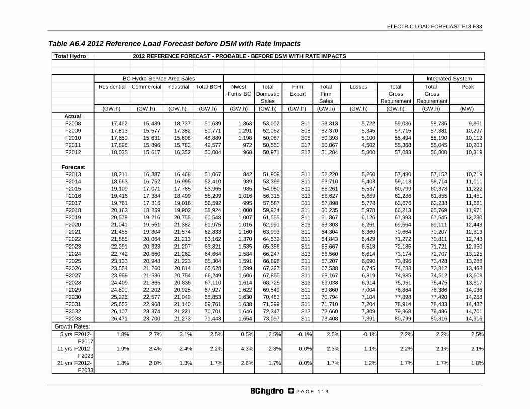
ELECTRIC LOAD FORECAST F13-F33
P A G E 1 1 3
Table A6.4 2012 Reference Load Forecast before DSM with Rate Impacts
Total Hydro 2012 REFERENCE FORECAST - PROBABLE - BEFORE DSM WITH RATE IMPACTS
Residential Commercial Industrial Total BCH Nwest Total Firm Total Losses Total Total PeakFortis BC Domestic Export Firm Gross Gross
Sales Sales Requirement Requirement(GW.h) (GW.h) (GW.h) (GW.h) (GW.h) (GW.h) (GW.h) (GW.h) (GW.h) (GW.h) (GW.h) (MW)
ActualF2008 17,462 15,439 18,737 51,639 1,363 53,002 311 53,313 5,722 59,036 58,735 9,861 F2009 17,813 15,577 17,382 50,771 1,291 52,062 308 52,370 5,345 57,715 57,381 10,297 F2010 17,650 15,631 15,608 48,889 1,198 50,087 306 50,393 5,100 55,494 55,190 10,112 F2011 17,898 15,896 15,783 49,577 972 50,550 317 50,867 4,502 55,368 55,045 10,203 F2012 18,035 15,617 16,352 50,004 968 50,971 312 51,284 5,800 57,083 56,800 10,319
ForecastF2013 18,211 16,387 16,468 51,067 842 51,909 311 52,220 5,260 57,480 57,152 10,719 F2014 18,663 16,752 16,995 52,410 989 53,399 311 53,710 5,403 59,113 58,714 11,011 F2015 19,109 17,071 17,785 53,965 985 54,950 311 55,261 5,537 60,799 60,378 11,222 F2016 19,416 17,384 18,499 55,299 1,016 56,315 313 56,627 5,659 62,286 61,855 11,451 F2017 19,761 17,815 19,016 56,592 995 57,587 311 57,898 5,778 63,676 63,238 11,681 F2018 20,163 18,859 19,902 58,924 1,000 59,924 311 60,235 5,978 66,213 65,769 11,971 F2019 20,578 19,216 20,755 60,548 1,007 61,555 311 61,867 6,126 67,993 67,545 12,230 F2020 21,041 19,551 21,382 61,975 1,016 62,991 313 63,303 6,261 69,564 69,111 12,443 F2021 21,455 19,804 21,574 62,833 1,160 63,993 311 64,304 6,360 70,664 70,207 12,613 F2022 21,885 20,064 21,213 63,162 1,370 64,532 311 64,843 6,429 71,272 70,811 12,743 F2023 22,291 20,323 21,207 63,821 1,535 65,356 311 65,667 6,518 72,185 71,721 12,950 F2024 22,742 20,660 21,262 64,664 1,584 66,247 313 66,560 6,614 73,174 72,707 13,125 F2025 23,133 20,948 21,223 65,304 1,591 66,896 311 67,207 6,690 73,896 73,428 13,288 F2026 23,554 21,260 20,814 65,628 1,599 67,227 311 67,538 6,745 74,283 73,812 13,438 F2027 23,959 21,536 20,754 66,249 1,606 67,855 311 68,167 6,819 74,985 74,512 13,609 F2028 24,409 21,865 20,836 67,110 1,614 68,725 313 69,038 6,914 75,951 75,475 13,817 F2029 24,800 22,202 20,925 67,927 1,622 69,549 311 69,860 7,004 76,864 76,386 14,036 F2030 25,226 22,577 21,049 68,853 1,630 70,483 311 70,794 7,104 77,898 77,420 14,258 F2031 25,653 22,968 21,140 69,761 1,638 71,399 311 71,710 7,204 78,914 78,433 14,482 F2032 26,107 23,374 21,221 70,701 1,646 72,347 313 72,660 7,309 79,968 79,486 14,701 F2033 26,471 23,700 21,273 71,443 1,654 73,097 311 73,408 7,391 80,799 80,316 14,915
Growth Rates: 5 yrs F2012- 1.8% 2.7% 3.1% 2.5% 0.5% 2.5% -0.1% 2.5% -0.1% 2.2% 2.2% 2.5%
F201711 yrs F2012- 1.9% 2.4% 2.4% 2.2% 4.3% 2.3% 0.0% 2.3% 1.1% 2.2% 2.1% 2.1%
F202321 yrs F2012- 1.8% 2.0% 1.3% 1.7% 2.6% 1.7% 0.0% 1.7% 1.2% 1.7% 1.7% 1.8%
F2033
BC Hydro Service Area Sales Integrated System