Eicher Begun EKC

8/4/2019 Eicher Begun EKC

http://slidepdf.com/reader/full/eicher-begun-ekc 1/34

In Search of a Sulphur Dioxide Environmental Kuznets Curve:

A Bayesian Model Averaging Approach*

Jeffrey Begun

University of Washington

Theo S. Eicher

University of Washington

Abstract

The exact specification and motivation of the Environmental Kuznets Curve (EKC) is the subject of a vastliterature in environmental economics. A remarkably diverse set of econometric approaches has beenemployed to support or reject a specific relationship between environmental quality and pollution. Nevertheless, methods employed to date have not addressed the issue of model uncertainty, given that asizable number of competing theories exist that can explain the income/pollution relationship.

We introduce Bayesian Model Averaging to the EKC analysis to examine a) whether a sulphur dioxideEKC exists, and if so, b) which income/pollution specification is most strongly supported by the data. Wefind only weak support for an EKC, which disappears altogether when we address oversampling issues inthe data. In contrast, our results highlight the relative importance of political economy and site-specificvariables in explaining pollution outcomes. Trade is also shown to play an important indirect role. It

moderates the influence of the composition effect on pollution. Our findings run contrary to thedeterministic view of the income/pollution relationship that is persistent in the literature.

*We thank Werner Antweiler and Bill Harbaugh for sharing their data and Chris Papageorgiou for comments.



2

I. Introduction

A vast empirical literature has sought to establish a robust relationship between economic

development and environmental quality. Grossman and Krueger (1995) and Selden and Song

(1994) examined the relationship and documented an inverted U-shaped curve between incomeand pollution that is similar to the inverted U-shaped relationship between income and inequality

first proposed by Kuznets (1955). The early data seemed to support an “environmental Kuznets

curve” (EKC) where initial phases of development are associated with increasing pollution while

richer nations experience improvements in their environmental quality.

Subsequently, however, a large number of authors have failed to confirm the EKC –

either in the original Grossman and Krueger dataset or in updated and expanded pollution

datasets (see, e.g., Harbaugh et al., 2002, or Deacon and Norman, 2006). The conflicting

empirical results have given rise to intense attempts either to formally model the EKC process

(see e.g., Antweiler et al., 2001), or to add further control variables to reduced-form regressions

to examine whether the EKC relationship can be resurrected and/or remain robust when the

model is correctly specified (see, e.g., Panatayotou, 1997).

The EKC is a case study of extreme model uncertainty where the true model is unknown

and several competing approaches exist to formalize the relationship between environmental

quality and income. In light of such model uncertainty, inference procedures based on only one

regression model overstate the precision of coefficient estimates since the uncertainty

surrounding the validity of a theory has not been taken into account (see Doppelhofer, 2005).

The problem is particularly prevalent in the EKC literature since a number of well-founded

approaches exist and researchers face an abundance of possible candidate regressors.

Bayesian Model Averaging (BMA) allows inferences to be based on a number of

competing models, each weighted by its quality. The procedure naturally delivers a posterior

distribution for each candidate regressor, whose mean is a smoothed estimate derived from all

relevant models. Hundreds of BMA papers have been published in the last decade as increases in

computing power allow end users to trawl through thousands of models mechanically in attempts

to address model uncertainty. In environmental economics, prominent examples of BMA

applications include the modeling of population determinants for deer and fish in Farnsworth et

al. (2006) and Fernandez, Ley and Steel (2002), respectively. To our knowledge, we are the first



3

to apply Bayesian Model Averaging to resolve the model uncertainty surrounding the EKC

relationship.

Our strategy is to group EKC approaches into two categories. First we examine reduced-

form approaches to the EKC, where many possible determinants of pollution are tested. Thenwe examine specific theories that have been proposed as the underlying determinants of an EKC,

and scrutinize how strongly the data supports theory-based candidate regressors. Before we

summarize our results, it is important to note that the updated S02 data that has been extended

and cleaned of previous errors no longer exhibits the EKC relationship that Grossman and

Krueger (1995) discovered (see, e.g., Harbaugh et al., 2002). Hence our results below can be

seen as an effort to find robust evidence for an EKC in this dataset by eliminating possible

omitted variable bias.

We find only limited evidence for an income/pollution relationship once we account for

model uncertainty in the data. Instead, robust and strongly related regressors in both reduced-

form and theory-based approaches are those relating to political economy, site-specific effect,s

and trade-induced composition effects. Societies that are more open in terms of political

participation are shown to exhibit significantly lower air pollution.

The theory-based approach highlights that the exact theoretical specification of the trade

effect on pollution matters. Following Antweiler et al. (2001), we show that the interaction

between trade and capital intensity is of crucial importance to explain the evolution of SO2

concentrations across countries and time. We also show that the composition effect has a

different impact on countries depending on their level of development. The greater the level of

development – as proxied by the human capital augmented capital-labor ratio – the lower the

implied concentrations for open economies. We also find support for pollution havens, since the

negative coefficient implies that countries with low capital intensity and high trade orientations

have higher pollution levels (see Birdsall and Wheeler, 1993).

It is important to note that the number of regressors that are robustly related to pollution

in the BMA approach, as well as the best model identified by BMA, contains only a fraction of

the 23 possible candidate regressors and only about one third of the 18 regressors suggested by

the most comprehensive theoretical specification in Antweiler et al. (2001). This provides

evidence that such a complex theory may not be necessary and alternative theories, such as the



4

Green Solow model, should not be discarded simply because they rely on only a fraction of the

regressors that Antweiler et al. (2001) introduced (see Taylor and Brock, 2003). Not only is the

number of robustly related regressors in BMA smaller than previous approaches suggested,

several are also not exclusively related to economic fundamentals.

Nevertheless, the best model suggested by BMA, which accounts for model uncertainty,

has an R-squared of 0.242 at the most disaggregated level, which is twice as high as Antweiler et

al.’s (2001) preferred full fixed-effects specification (R 2 = 0.15). Indeed, the best model

identified in our preferred specification, which also addresses the severe oversampling issues in

the data, features an R-squared of 0.514. This implies that the significance of the large number of

regressors in previous theory-based and reduced-form regressions may be an artifact of an

approach that did not take into account model uncertainty.

2) The SO2 EKC

2.1) Data Considerations

Perhaps the most salient EKC relationship in the literature is between air quality and

development.1 In this paper we focus on median sulphur dioxide (SO2) concentration data from

the Global Environmental Monitoring System (GEMS) to search for an EKC. The data is

updated, error-corrected and maintained by the EPA in its Aerometric Information Retrieval

System (AIRS).2

The GEMS/AIRS data is perhaps the most widely used dataset to investigatethe EKC, with reported SO2 concentrations from stations in up to 44 countries from 1971 to

2006.3

However, most of the data since the early 1990s exists only for the United States.

Our income measure is real GDP per capita in constant 1996 dollars from the Penn World

Tables 6.1 (Heston, Summers and Aten, 2002). In a later section when we compare results to

Antweiler et al. (2001, subsequently referred to as ACT), we also use their GNP data as an

income measure. We use concentration data, although emissions data is also widely available,

1 Alternative measures have been used. Evidence for an EKC has been found for water quality (Grossman andKrueger, 1995), deforestation (Cropper and Griffith, 1994; Panayotou, 1995) and water withdrawal for agriculture(Rock, 1998; Goklany, 2002). Some researchers have found an EKC for carbon dioxide (Roberts and Grimes, 1997)though others have found that CO2 increases monotonically with income (Shafik and Bandyopadhyay, 1992).2 Our raw GEMS/AIRS data is identical to Antweiler, Copeland and Taylor (2001), who kindly shared their data thatincludes median concentrations.3 See, for example, Grossman and Krueger (1995), Panayotou (1997), Torras and Boyce (1998), Barrett and Graddy(2000), Harbaugh et al. (2002) and Deacon and Norman (2006).



5

because it is the concentration of SO2 in the atmosphere that matters for the environmental

impact.

The SO2 data is, however, highly unbalanced in two dimensions: location and time. Few

countries report data over the entire time period, and many countries report pollutionconcentrations for less than a decade. Often entire years of data are missing between

observations not only on the station level, but also on the city and country level. Even in

countries with extensive locational coverage, such as the United States, the time series for each

monitoring station is highly unbalanced.

The data are unbalanced in terms of location since a few countries are represented with

large numbers of reporting stations, while many other nations feature only one. A full 38 percent

of the original 2,555 station-level observations originate in the U.S. and Canada. The imbalance

is exacerbated early and late in the sample as the U.S. supplies 69 percent of the data before 1974

and after 1993. Therefore we restrict our analysis to 1994-1993, which reduces the dataset by

219 mostly U.S. observations. The literature has largely been concerned with documenting the

EKC (or the absence thereof) without acknowledging the fact that the dataset is so extremely

unbalanced. In Section 2.2 we discuss measures to balance the sample, which require us to drop

seven countries with a total of 128 observations because they lacked either SO2 or PWT 6.1 for

at least two five-year periods.4

Finally, we had to drop Hong Kong (40 observations) because it

lacked the Polity IV data described below, and Yugoslavia was dropped by ACT because it lacks

human capital data. Figure 1 provides a breakdown of the 2168 observations by country of

origin.

2.2 The EKC in the Raw Income Pollution Data

As mentioned in section 2.1, we employ the same GEMS dataset for income and sulphur dioxide

pollution that has been used extensively in the previous literature. Starting with the very first

paper by Grossman and Krueger (1991) and continuing on to perhaps the most prominent recent

work on the income/pollution relationship by ACT, this dataset has been the cornerstone of EKC

support. The first surprise for researchers using the newest version of GEMS, which has been

purged of errors and extended to include updated data, is that it no longer provides evidence for

4 These countries (and their number of observations) are Austria (2), Kenya (4), Switzerland (2), Ghana (3), CzechRepublic (21), Poland (86) and Iraq (9). Iraq and Poland are excluded only when we use GDP measures. A completedescription of the data used in this paper is provided in the appendix.



6

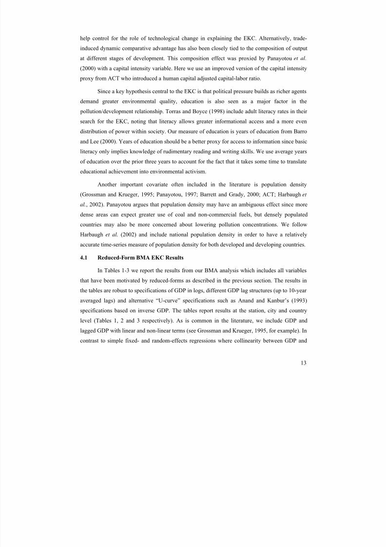
the fundamental EKC relationship. Figure 2 plots the raw data for every station in every year

that an observation is recorded. In addition, the figure traces the predicted values from the most

fundamental regression that includes only log SO2 concentrations as the dependent variable and

real GDP per capita as a third-order polynomial.5

In Grossman and Krueger (1995), a similar plot

was prominently inverted-U shaped.

Instead of an EKC, the updated GEMS data in Figure 2 shows a simple relationship

between development and environmental quality that has SO2 concentrations gradually declining

with income. The lack of an EKC in the raw SO2 data has previously been noticed by astute

researchers who suggested that global data masks country-level phenomena. Deacon and

Norman (2006) provide strong evidence that the country-level experience may in fact look very

different from the global station-level data. Since technology, factor abundance and the political

response to interest groups are also national concepts, we aggregate the data in search of an EKC

at the individual country level. Figure 3 confirms Deacon and Norman’s (2006) results by

plotting country-level SO2 concentrations over time and showing that most countries’ SO2

concentrations do not follow an EKC path. In fact, it is difficult to discern any country in Figure

3 that exhibits the single peak predicted by the EKC hypothesis. Indeed, Deacon and Norman

(2006) show that diverse SO2 –income relationships exist among countries; depending on the

nation, rising income may be associated with rising, falling or stable SO2 concentrations.

The lack of an EKC at the station or individual country level might be an artifact of the

extremely unbalanced time- and location-dimensions of the dataset. Since our main explanatory

variable, real GDP per capita, is defined at the country level, oversampling in countries with

multiple reporting stations may bias the station-level regressions severely. To balance the

sample, we follow Selden and Song (1994) and take five-year averages that correct for much of

the time and locational imbalances discussed in Section 2.1. In the averaged dataset, the U.S.

prominence is reduced to 24 percent of the observations at the station-level. Therefore, averaging

helps address our oversampling concerns, and in the country-level data the entire locational

5 We employ fixed-effects regressions throughout. It has been argued that the random effects EKC cannot beestimated consistently (Mundlak, 1978; Hsiao, 1986; Stern, 2003). Since the very premise of the EKC is thatspecific local, regional or national characteristics are crucial, the random-effects approach suffers frominconsistency due to omitted variables. In addition, we have no desire to imply that a possible EKC in our data holds beyond the countries in this sample. Hence, we take the view that countries represented are not simply randomdraws from a larger EKC country/station population. An additional advantage of the fixed-effects approach is that itcontrols for many time-invariant, site-specific and country-specific factors.



7

imbalance that leads to oversampling concerns is eliminated. Averaging data over five-year

intervals is also common in the economic growth literature and allows us to address the error

associated with business cycle fluctuations that are inherent in income data (see Barro, 1990).

Nevertheless, we will continue to examine and report results for all three levels of aggregation.

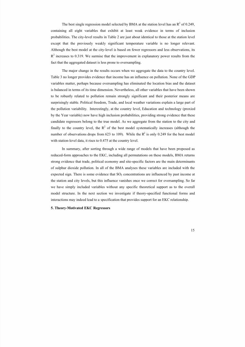
Averaging across time and aggregating by country does not resolve the mystery of the

missing EKC in the raw data, however. Plotting the station-level data and the predicted values

obtained by the same method as in Figure 2, the country-level data in Figure 4 maintains the

negative relationship between pollution and income. The monotonic decline is a bit surprising

given past support for an EKC in the GEMS data (e.g., Shafik, 1994; Grossman and Krueger,

1995; Torras and Boyce, 1996; Panayotou, 1997). A careful study by Harbaugh, Levinson and

Wilson (2002) with the revised GEMS/AIRS data, however, found evidence that sulphur dioxide

concentrations may initially decline as income rises. In addition, Perman and Stern (2003), who

use the same data and make adjustments for previous methodological and data problems with

appropriate statistical techniques, also found no EKC evidence. Given the heterogeneity

observed in Figure 3, and the results of Deacon and Norman (2006), our station-level results are

not surprising.

3. Model Uncertainty in the Income / Environment Relationship

Two simple explanations can address the absence of an EKC in the raw data presented in

Figures 2 and 4. Either the relationship does not exist, or the model is misspecified. By

neglecting to include crucial covariates, the misspecification due to omitted variable bias may

overwhelm the power of the GDP regressors. Perhaps in an effort to explore the latter line of

reasoning, the literature features a remarkably diverse range of different model specifications to

uncover evidence in favor of an EKC.

Below, we first focus on the most prominent reduced-form approaches that commonly

include variables to sharpen the EKC model specification such as international trade, capital

intensity, precipitation variation, temperature, population density, investment, education,

institutions, and interaction terms. Instead of juxtaposing various versions of different

researchers’ preferred models as is standard in robustness analysis, we use an advanced model

selection technique to address the model uncertainty inherent in the EKC literature. Bayesian

Model Averaging (BMA) is the most sophisticated and theoretically grounded method to address



8

model uncertainty. The next section provides a brief abstract of the BMA method and identifies

how the procedure resolves EKC model uncertainty.

3.1 Addressing Model Uncertainty in the Income / Environment Relationship

The issue of model uncertainty in general has long been recognized as a major problem in

economics. When inferences are based on one model alone, the ambiguity involved in model

selection dilutes information about effect sizes and predictions since “part of the evidence is

spent to specify the model” (Leamer, 1978, page 91). It is therefore not surprising that averaging

over all models can be proven to provide better average predictive performance than just picking

any single model (Madigan and Raftery, 1994).

The basic model averaging idea originated with Jeffreys (1961) and Leamer (1978),

whose insights were developed and operationalized by Draper (1995) and Raftery (1995). BMA

was first introduced to economics by Fernandez, Ley and Steel (2001), with an application to

economic growth. Here we restrict ourselves to sketching the basic BMA structure before we

discuss the results (for an extensive discussion of BMA see Hoeting, Madigan, Raftery and

Volinsky, 1999). Environmental applications of BMA include (among many others) Farnsworth

et al. (2006) and Fernandez, Ley and Steel (2002).

Consider n independent replications from a linear regression model. The dependent

variable (S02 pollution) in n countries grouped in vector γ is regressed on an intercept α and a

number of explanatory variables chosen from a set of k candidate regressors contained in a

design matrix Z of dimension n x k . Assume that ( ) 1: += k Z r nι , where ( )⋅r indicates the

rank of a matrix and nι is an n -dimensional vector of ones. Further define β as the full k -

dimensional vector of regression coefficients.

Now suppose that we have a jk n× submatrix of variables in Z denoted by . j Z Then

denote by j M the model with regressors grouped in , j Z such that

,σε β αι ++= j jn Z y

where j β jk ℜ∈ )0( k k j ≤≤ groups regression coefficients corresponding to the submatrix j Z ,

+ℜ∈σ is a scale parameter, and ε is a random error term that follows an n -dimensional



9

normal distribution with a zero mean and an identity covariance matrix. Exclusion of a regressor

in a particular model implies that the corresponding element of β is zero. Since we allow for

any subset of variables in Z to appear in each model, j M , there exist k 2 possible sampling

models.

Given this setup, BMA implies that the posterior probability of any given parameter of

interest, ,∆ has a common interpretation across models. It is the weighted posterior distribution

of ∆ under each of the models, with weights given by the posterior model probabilities, or

( ).|,|

1

2

| y M PPP j M y

j

y j

k

∆=

∆ ∑= (1)

That is, the marginal posterior probability of including a particular regressor is the weighted sum

of the posterior probabilities of all models that contain the regressor. The posterior model

probability for Model M j is given by

,

)(

)()|(

1

2

hh yh

j j y

j

p M l

p M l y M P

k

=∑

= (2)

where )( j y M l , is the marginal likelihood of model j M given by

,),,|(),(),,,|()( σ β α σ α β σ α σ β α d d d M p p M y p M l j j j j j j y ∫ =

Note that ),,,|( j j M y p σ β α is the sampling model corresponding to equation (1), and ),( σ α p

and ),,|( j j M p σ α β are the priors of the intercept and the regressors, respectively.

Thus, BMA does not rely on any individual model to generate inferences, but provides a

posterior distribution for each estimate. BMA thus bases the inference on the weighted average

of a selection of models. The weights themselves are given by a measure of the quality of each

individual model relative to all other models. BMA therefore constitutes an intuitively attractive

solution to model uncertainty as it considers all possible models and generates an average that is

dominated by models which receive the greatest support from the data.

Despite its theoretical rigor and power of inference, BMA has not yet become part of the

standard data analysis tool kit. This has been due to several early difficulties in implementing



10

BMA. First, the number of terms in equation (1) can be enormous, rendering exhaustive

summation infeasible. This problem has recently been addressed by an efficient search algorithm

incorporated into the Raftery et al. (1997) “bic.reg” routine.6 The routine guarantees that the

best model is found, while alternative samplers such as MC3 (Madigan et al., 1995) or the totally

random coin flip sampler (Sala-i-Martin, Doppelhofer and Miller, 2003) do not provide such an

efficient search.

Much more problematic for BMA has been the Bayesian requirement to specify prior

distributions for all parameters in all competing models. An extensive discussion on the

significance of priors in BMA is provided by Fernandez, Ley and Steel (2001) and in Eicher,

Papageorgiou and Raftery (2006). In our application of BMA below, we utilize priors that are

among the most conservative and diffuse Bayesian priors. The unit information prior employed

below is so diffuse and uncontroversial that it can be derived from frequentist statistics.7

4. Reduced-Form Approaches to the EKC

Before we can employ BMA, we must motivate the various candidate regressors that are

to be included alongside the GDP measures. A number of covariates have been introduced in the

past to explain sulphur dioxide concentrations. These regressors can be grouped into five

different categories: 1) site-specific controls, 2) political economy proxies, 3) production

structure, 4) trade measures, and 5) technology proxies. We discuss each one in detail below.

Stations from 44 countries around the world report sulfur dioxide concentrations in the

GEMS/AIRS data. A compelling argument can be made that any analysis of the income-

pollution relationship must include regressors that control for site-specific factors. Examples of

regional variations that may explain sulphur dioxide concentrations in the vicinity of a measuring

station would be specific weather conditions (temperature and precipitation) or topographical

features. Such regional differences affect nature’s ability to cleanse sulphur dioxide from the

atmosphere. While variables such as Temperature, Precipitation Variation, and topographic

features are unlikely to be correlated with our economic variables, their inclusion is standard in

the literature and meant to improve the accuracy of the estimates. Our site-specific controls are

6 The software can be freely obtained from http://www.research.att.com/~volinsky/software/bicreg.7 The unit information prior is a multivariate normal prior with mean at the maximum likelihood estimate andvariance equal to the expected information matrix for one observation (Kass and Wasserman, 1995). It can bethought of as a prior distribution that contains the same amount of information as a single, typical observation.



11

obtained from ACT, who include average monthly temperatures for each reporting station to

capture seasonal influences on the demand for fuels (and hence SO2 concentrations), and to

account for the fact that higher temperatures allow SO2 to dissipate pollution more rapidly. We

also include the variation in precipitation at each site from ACT since seasonally-concentrated

rainfall reduces the region’s ability to dissipate SO2 over the year. In addition, we add a dummy

for nations who signed the 1985 Helsinki Protocol, which aimed to reduce sulphur emissions by

at least 30 per cent.8

Before we turn to economic covariates, we must also control for common-to-world but

nevertheless time-varying components. Such components are included to reflect secular changes

in global awareness of environmental problems, innovations and diffusion of abatement

technology, and the evolution of world prices. We follow the standard practice in the literature

and seek to capture such common components with a linear time trend.

A number of studies have extended the pure EKC specification to include additional

explanatory variables that may be tied to both pollution and economic development. Clearly

income alone does not create pressure to improve environmental outcomes; the democratic fabric

of a society that allows political participation and threatens consequences to polluting dictators is

also seen as an important determinant. Hence the past literature introduced variables to account

for the fact that more open and democratic societies may have different attitudes towards the

environment. The conjecture is that for a given level of income, more open societies experience

less pollution.

Many specific mechanisms for this to take place have been identified in the literature.

Torras and Boyce (1998) posit that richer individuals gain “power” to demand better overall

environmental quality. Likewise, Barrett and Graddy (2000) propose that wealthier citizens

demand an increase in the non-material aspects of their standard of living. The degree to which

policy responds to such desires is closely linked to the ability of individuals to assemble,

organize and voice their concerns. In the same vain, Panatayotou (1997) provides evidence that

strong property rights “flatten” the EKC by generating less pollution for any given income level.

8 Much of the previous research, starting with Grossman and Krueger (1993, 1995), also includes site-geographyvariables such as proximity to oceans or deserts. Our fixed-effects regressions account for these implicitly.



12

Several different measures of political rights and civil liberties have been used in the

literature. Some authors have employed the Freedom House indices (e.g., Shafik and

Bandyopadhyay, 1992; Torras and Boyce, 1998; Barrett and Graddy, 2000) while others such as

Panayotou (1997) use “Respect/Enforcement of Contracts” from Knack and Keefer (1995). More

recently Harbaugh et al. (2002) use an index of democratization from the Jaggers and Gurr

(1995) Polity III dataset. Alternatively, Leitão (2006) introduces measures of corruption to

examine how diversion activities may affect an EKC. The institutions and growth literature has

since established the use of the “Constraint on Executive” variable from the updated Marshall

and Jaggers (2003) Polity IV database as perhaps the best measure to capture the above

mentioned effects. Acemoglu et al. (2001) have shown convincingly that the degree of constraint

on the executive is a fundamental determinant of all political rights. We thus choose this measure

as our political rights proxy.9

International trade has also been associated with the EKC relationship. Taylor and Brock

(2004) survey the literature, highlighting an early contention by Arrow et al. (1995) and Stern et

al. (1996) that an EKC might be partly or largely due to trade and its implied global distribution

of polluting industries. Following the Heckscher-Ohlin model, the authors hypothesized that free

trade allows developing countries to specialize in goods that are intensive in their relatively

abundant factors: labor and natural resources. Developed countries, in turn, are likely to

specialize in human capital and capital intensive goods. Following ACT, we use trade volume

(exports plus imports) as a percent of GDP as our measure of openness to trade.

In contrast, Shafik and Bandyopadhyay (1992) point out that trade might exert two

contrasting influences on developing countries. First, there exists the above effect where

developing countries have an environmental comparative advantage due to low environmental

protection costs, which leads to the intense manufacture and export of pollution-intensive goods.

On the other hand, increased openness may lead to increased competition, which could cause

more investment in efficient and cleaner technologies that meet the environmental standards of developed nations. To control for potentially opposing forces, we follow Harbaugh et al. (2002)

and include not only trade, but also a measure of investment in our analysis. To the extent that a

portion of investment leads to cleaner manufacturing processes, including investment should

9 Note that the literature has clearly established the absence of a direct democracy/income relationship (Acemoglu et

al., 2005). Hence we do not interpret our political economy measure as a proxy for income.



13

help control for the role of technological change in explaining the EKC. Alternatively, trade-

induced dynamic comparative advantage has also been closely tied to the composition of output

at different stages of development. This composition effect was proxied by Panayotou et al.

(2000) with a capital intensity variable. Here we use an improved version of the capital intensity

proxy from ACT who introduced a human capital adjusted capital-labor ratio.

Since a key hypothesis central to the EKC is that political pressure builds as richer agents

demand greater environmental quality, education is also seen as a major factor in the

pollution/development relationship. Torras and Boyce (1998) include adult literacy rates in their

search for the EKC, noting that literacy allows greater informational access and a more even

distribution of power within society. Our measure of education is years of education from Barro

and Lee (2000). Years of education should be a better proxy for access to information since basic

literacy only implies knowledge of rudimentary reading and writing skills. We use average years

of education over the prior three years to account for the fact that it takes some time to translate

educational achievement into environmental activism.

Another important covariate often included in the literature is population density

(Grossman and Krueger, 1995; Panayotou, 1997; Barrett and Grady, 2000; ACT; Harbaugh et

al., 2002). Panayotou argues that population density may have an ambiguous effect since more

dense areas can expect greater use of coal and non-commercial fuels, but densely populated

countries may also be more concerned about lowering pollution concentrations. We follow

Harbaugh et al. (2002) and include national population density in order to have a relatively

accurate time-series measure of population density for both developed and developing countries.

4.1 Reduced-Form BMA EKC Results

In Tables 1-3 we report the results from our BMA analysis which includes all variables

that have been motivated by reduced-forms as described in the previous section. The results in

the tables are robust to specifications of GDP in logs, different GDP lag structures (up to 10-year

averaged lags) and alternative “U-curve” specifications such as Anand and Kanbur’s (1993)

specifications based on inverse GDP. The tables report results at the station, city and country

level (Tables 1, 2 and 3 respectively). As is common in the literature, we include GDP and

lagged GDP with linear and non-linear terms (see Grossman and Krueger, 1995, for example). In

contrast to simple fixed- and random-effects regressions where collinearity between GDP and



14

lagged GDP variables might compromise the explanatory power of either variable, BMA

averages across relevant models and thus potentially mitigates the effects of collinearity.

The first column of each table reports the posterior inclusion probability, P, which

indicates the probability that the coefficient estimate is different from zero.

10

P≠

0 is thus ameasure of confidence of including a candidate regressor with non-zero coefficient in the true

regression model. The posterior inclusion probability has the additional advantage that it is a

scale-free probability measure of the relative importance of the variables, which can therefore be

transparently applied for policy decisions and inference, in addition to the posterior mean and

standard deviation. Jeffries (1961) and Raftery (1995) add the additional interpretational

refinement that P ≠ 0 > 50 percent suggests that the data provides weak evidence that the

regressor is included in the true model; P ≠ 0 > 75 percent implies positive evidence; P ≠ 0 > 95

percent provides strong evidence; and P ≠ 0 > 99 percent gives very strong evidence. Inclusion

probabilities close to 100 percent signal that the particular regressor is included in almost all

good models, and that it contributes prominently to explaining the dependent variable even in the

presence of significant model uncertainty.

Overall, we find only limited support for income as a key driver of SO2 concentrations.

Only the highly unbalanced datasets at the station and city level (Tables 1 and 2) report positive

evidence of an EKC relationship between income and SO2 concentrations (the GDP data is in

$10,000). Table 1 shows that lagged GDP has a much higher inclusion probability than current

GDP, implying that contemporaneous economic activity is much less important in determining

SO2 concentrations than the indirect effects of rising income over time that may proxy for

changes in technology. Nevertheless, fundamental variables, not income, are the most relevant

for explaining pollution levels. Precipitation Variation and Executive Constraints both have 100

percent inclusion probabilities, while the income polynomials range around 80 percent. We find

that less variation in precipitation, increased temperatures, and greater constraints on the

country’s chief executive reduce sulphur dioxide concentrations. The only economic variablethat registers as significant in the reduced-form station level results is Trade Intensity. Here the

evidence is decisive that trade reduces pollution.

10 In contrast to frequentist statistics, where one null and one alternative model is implied, BMA considers all possible models, hence simple t-values are not appropriate. Indeed, Raftery (1995) notes that the theory of t-valueswas developed for the comparison of two nested models and in a typical structural equation model application, suchas the EKC, there may be many substantively meaningful models (many of them non-nested).



15

The best single regression model selected by BMA at the station level has an R 2 of 0.249,

containing all eight variables that exhibit at least weak evidence in terms of inclusion

probabilities. The city-level results in Table 2 are just about identical to those at the station level

except that the previously weakly significant temperature variable is no longer relevant.

Although the best model at the city-level is based on fewer regressors and less observations, its

R 2

increases to 0.319. We surmise that the improvement in explanatory power results from the

fact that the aggregated dataset is less prone to oversampling.

The major change in the results occurs when we aggregate the data to the country level.

Table 3 no longer provides evidence that income has an influence on pollution. None of the GDP

variables matter, perhaps because oversampling has eliminated the location bias and the dataset

is balanced in terms of its time dimension. Nevertheless, all other variables that have been shown

to be robustly related to pollution remain strongly significant and their posterior means are

surprisingly stable. Political freedom, Trade, and local weather variations explain a large part of

the pollution variability. Interestingly, at the country level, Education and technology (proxied

by the Year variable) now have high inclusion probabilities, providing strong evidence that these

candidate regressors belong to the true model. As we aggregate from the station to the city and

finally to the country level, the R 2

of the best model systematically increases (although the

number of observations drops from 623 to 109). While the R 2 is only 0.249 for the best model

with station-level data, it rises to 0.475 at the country level.

In summary, after sorting through a wide range of models that have been proposed as

reduced-form approaches to the EKC, including all permutations on these models, BMA returns

strong evidence that trade, political economy and site-specific factors are the main determinants

of sulphur dioxide pollution. In all of the BMA analyses these variables are included with the

expected sign. There is some evidence that SO2 concentrations are influenced by past income at

the station and city levels, but this influence vanishes once we correct for oversampling. So far

we have simply included variables without any specific theoretical support as to the overallmodel structure. In the next section we investigate if theory-specified functional forms and

interactions may indeed lead to a specification that provides support for an EKC relationship.

5. Theory-Motivated EKC Regressors



16

Second-generation EKC models include not only variables motivated by heuristic,

reduced-forms, but also fully specified models that yield precise, testable EKC implications and

relationships. The essential features of the models include the determinants of scale,

composition, and technique effects outlined by Panayotou (1997) and discussed in extensive

detail by Taylor and Brock (2004). Prominent theoretical precursors that have led to the state of

the art, fully specified, open-economy EKC model in ACT are Stokey (1998) (endogenous

abatement), Bovenberg and Smulders (1995) and Aghion and Howitt (1998) (endogenous

growth/technique), and Jones and Manuelli (2001) (endogenous policy). We direct the interested

reader to the excellent Taylor and Brock survey and address only cornerstones of the theoretical

EKC models that are relevant to empirical investigation.

All models that examine the development/pollution relationship make implicit

assumptions regarding the strength of three different (and potentially offsetting) effects. First,

development causes a positive scale effect since increased output per unit of capital leads to

increased pollution. To account for the scale effect we follow ACT and employ a measure of

city-level economic intensity (national GDP per capita times city population density). It is

generally held that in rapidly growing middle-income countries pollution due to the scale effect

might be the dominant EKC force (Perman and Stern 2003).

Second, a technique effect diminishes the scale effect as technological progress permits a

lowering of emissions per unit of output. Lagged per capita income is used to proxy for the

technique effect since countries with higher incomes in the past should be able to afford better

technology today (see ACT). Diffusion of technology itself motivates the idea that time-related

effects reduce environmental impacts in countries at all levels of development (Aghion and

Howitt, 1998, Perman and Stern, 2003). These effects are usually proxied with a year dummy.

To isolate either the scale or technique effect, we must control for changes in the

composition of output. A change in output composition can mitigate the scale effect further if the

share of less pollution-intensive industries rises as income increases. This occurs when

development and human capital accumulation generate shifts toward cleaner industries (services

or information technology) and an ensuing change in the composition of output that then reduces

environmental degradation (Panayotou, 1993). A specific model was first presented by Copeland

and Taylor (2003), who showed that the reliance on capital accumulation in early stages of



17

development, as opposed to human capital accumulation in later stages, can also generate an

EKC. We capture the composition effect by controlling for differences in the capital-labor ratio

that is adjusted for human capital, following ACT. In the absence of such controls, the pollution-

income relationship is a mixture of scale, composition, and technique effects, which is hard to

interpret.

In addition to a simple income/output-induced composition effect, ACT also take into

account a trade-induced composition effect. As discussed in the reduced-form literature, the

effect of trade on pollution can be ambiguous. In ACT the trade-induced composition effect

depends on the country’s comparative advantage, which in turn is determined by income per

capita and capital abundance. In moving from theory to practice, ACT suggest interacting the

trade measure with determinants of comparative advantage (the capital-labor ratio and income

per capita). Since comparative advantage is a relative concept, these are measured relative to the

corresponding world averages. Since theory cannot identify a turning point (at what level of

endowment trade causes a switch from exporting to importing pollution-intensive products), we

adopt the flexible approach of ACT by estimating interactions with different functional forms.

To allow BMA to replicate the ACT results, we include a site-specific dummy for

communist regimes which we interact with income per capita. This allows for a unique

pollution-income dynamic in communist nations where political participation is extremely low.

We can then test whether communist regimes are inherently disinterested in a public desire for a

cleaner environment. Essentially we have already introduced a variable that proxies for the

political economy effects with Executive Constraints, but BMA is exactly the appropriate

statistical framework to elicit which one (if any) of these proxies influences pollution.

It is important to note that theory does not necessarily imply such an elaborate structure.

As mentioned in the introduction, Taylor and Brock (2004) meticulously outline that the EKC is

compatible with many different underlying mechanisms and theories. The simplest of all is

perhaps the environment augmented “Green Solow model” where pollution policy remains

unchanged throughout the development process and where transitional dynamics alone suffice to

generate an EKC. The Green Solow model exhibits no composition effects, no changes in

pollution abatement, no evolution of the political process and no international trade. Hence the

Green Solow model is compatible with no change in trade or pollution policy as the country





19

station, city or country level. Nevertheless, the BMA results do suggest that Trade plays an

important indirect role in determining pollution. The correct specification of the trade effect as

outlined by the ACT theory is crucial. Here BMA reveals that the importance of Trade lies in its

power to moderate the composition effect.

ACT find that Trade moderates the pure EKC effect as the trade/income interactions in

their regression are highly significant. In the BMA approach, in contrast, this is income effect is

confirmed only at the station level (ACT’s level of aggregation). In the less unbalanced city- and

country-level datasets, BMA indicates that Trade’s sole role is to moderate the composition

effect. The interaction between Trade and Capital Intensity shows that the composition effect has

a different impact on countries depending on their level of development. The greater the level of

development – as proxied by the human capital augmented capital-labor ratio – the lower the

implied concentrations for open economies. The capital intensity variable has been included in

the past to control for development-contingent shifts towards cleaner technologies; while it

exhibited the same sign in ACT, it was statistically insignificant. The variable also provides

support for pollution havens, since the negative coefficient implies that countries with low

capital intensity and high trade orientations have higher pollution levels.

The second trade-related variable that receives strong support in BMA at all levels of

aggregation is the interaction between Trade, GDP, and Capital Intensity. Interestingly, this

variable is the one regressor that is estimated with just about the same coefficients and high level

of significance in ACT as in BMA. The positive estimate throughout thus provides strong

evidence that more human/physical-capital-intensive countries have higher sulphur dioxide

concentrations, even after we control for trade and income effects. This is because the three-way

interaction between Trade, GDP, and the Human Capital adjusted capital-labor ratio has a

positive posterior mean. The relatively large role of the composition effect and the trade-based

interactions suggests that countries do not follow a deterministic income-pollution path. Recall

that Figure 3 highlights the variety of country-specific pollution paths as incomes rise.

In contrast to ACT, BMA does not find evidence for a pure composition effect as capital

intensity alone cannot be shown to affect pollution. In addition, despite our efforts to control for

possible contamination of the scale effect, BMA provides no evidence that scale effects matter at

the station level (the scale effect was only mildly significant in ACT’s work). Oversampling does



20

influence the strength of the technique effect (proxied by Year), as BMA provides strong

evidence that a technique effect reduces pollution at the country level. A similar pattern was

observed in our reduced-form analysis, where the same variable gained explanatory power only

at higher levels of aggregation. These findings are in line with Stern and Common (2001) and

Stern (2002) who find evidence for the important role of negative time effects in explaining

declining SO2 concentrations.

It is important to note that the best model chosen by BMA contains about a quarter of the

23 candidate regressors that have been motivated by the literature. At the station level, six

highly significant regressors account for about twice the variation in the dependent variable (R 2 =

0.242) as the 18 regressors (13 significant) suggested by the ACT specification (R 2 = 0.15). This

could imply that a number of regressors identified by ACT may be significant only because the

empirical strategy did not account for model uncertainty. The estimates at different levels of

aggregation are surprisingly stable, however, and their R 2

increases steadily from station, city, to

country levels, from 0.24 to 0.34 to 0.51, respectively. Also, the relevant regressors at the city

and station level are just about identical, although the country-level results do feature two

additional regressors to explain pollution (Year and Education). The coefficient on Education is

counterintuitive just as in the reduced-form BMA results. It is supposed to proxy for the

hypothesis that better-educated citizens demand better environmental quality. However,

measures of education have been shown to be fragile in both growth regressions and in

development accounting (see Krueger and Lindahl, 2001). Perhaps the same issues contaminate

the effect of the regressors here.

VI. Conclusion

This paper reexamines the evidence for an environmental Kuznets curve using the most

recent EPA data on SO2 concentrations. The literature on the income-pollution relationship is

vast and characterized by unusual model uncertainty as both the number of proposed theories and

the range of possible candidate regressors is massive when it comes to empirical validation. We

apply a theoretically founded method to address model uncertainty. Bayesian Model Averaging

examines all models, weighs them by their relative quality, and then generates a probability that

a candidate regressor is related to the dependent variable.



21

Our results are presented at three levels of aggregation. The station-level results are

subject to severe oversampling as pollution from thousands of observations from local stations

are linked to one and the same measure of income in a country. Hence we also aggregate the data

to the city and country level. The results are remarkably robust. Political economy and site-

specific variables explain a large share of the observed pollution. International trade is also

shown again and again to be robustly related to pollution. In our reduced-form analysis, trade is

found to lower pollution. When the model is specified using full-fledged theory, we show that

trade has no direct effect, but that it moderates the composition effect. As countries become

richer and increase their physical and human capital, trade leads to cleaner environments. It

unfortunately also implies that poor, labor-intensive, open economies experience increasing

pollution levels.

Overall, we find only weak evidence for an EKC, which disappears when we address

oversampling of the data or move to a theory-based analysis. There may be several reasons the

EKC fails to hold up in our work. The foremost, perhaps, is that many countries in the time

period covered by the GEMS/AIRS data may already be on the flat or the downward sloping

portion of the EKC during the sample period. Smulders, Bretschger and Egli (2005) label these

portions of the EKC the “alarm phase” and the “cleaning-up phase” that indicate government

response to public concerns. Given that the rate of emissions reduction may also be based on

governments reacting to their citizens’ demands, it is not surprising that we find that policy

variables such as Executive Constraints play a crucial role in determining pollution levels.



22

References

Acemoglu, D., S. Johnson, and J. A. Robinson (2001), ‘The colonial origins of comparativedevelopment: an empirical investigation’, American Economic Review 91(5): 1369-1401.

Acemoglu, D., S. Johnson, J.A. Robinson, and P. Yared (2005), ‘From education to democracy?’ American Economic Review 95(2): 44-49.

Aghion, P. and P. Howitt (1998), ‘Capital accumulation and innovation as complementaryfactors in long-run growth’, Journal of Economic Growth 3: 111-130.

Anand, S. and S.M.R. Kanbur (1993), ‘Inequality and development: a critique’, Development

Economics 41: 19-43.

Antweiler, W., B.R. Copeland, and M.S. Taylor (2001), ‘Is free trade good for the environment?’ American Economic Review 91: 877-908.

Arrow, K., B. Bolin, R. Costanza, P. Dasgupta, C. Folke, C.S. Holling, B-O Jansson, S. Levin,

K-G Mäler. C. Perrings, and D. Pimentel (1995), ‘Economic growth, carrying capacity, andthe environment’, Science 268: 520-521.

Barrett, S. and K. Graddy (2000), ‘Freedom, growth, and the environment’, Environment and

Development Economics 5: 433-456.

Barro, R. J. (1990), ‘Government spending in a simple model of endogenous growth’, Journal of

Political Economy 98: S103-S125.

Barro, R. J. and J-W Lee (2000), ‘International data on educational attainment: updates andimplications’, CID Working Paper No. 42.

Birdsall, N. and D. Wheeler (1993), ‘Trade policy and industrial pollution in Latin America:where are the pollution havens?’ Journal of Environment and Development 2(1): 137–149.

Bovenberg, A.L. and S. Smulders (1995), ‘Environmental quality and pollution-savingtechnological change in a two-sector endogenous growth model’, Journal of Public


Cole, M.A. (1999) ‘Limits to growth, sustainable development and environmental Kuznetscurves: an examination of the environmental impact of economic development’, Sustainable

Development 7(2): 87-97.

Copeland, B.R. and M.S. Taylor (2003), ‘Trade and the Environment: Theory and Evidence’,Princeton, N.J.: Princeton University Press, 2003.

Copeland, B.R. and M.S. Taylor (2004), ‘Trade, growth, and the environment’, Journal of

Economic Literature 42(1): 7-71.

Cropper, M. and C. Griffiths (1994), ‘The interaction of population growth and environmentalquality’, American Economic Review 84: 250-254.

De Bruyn, S.M., J.C.J.M. van den Bergh, and J.B. Opschoor (1998), ‘Economic growth andemissions: reconsidering the empirical basis of environmental Kuznets curves’, Ecological




23

Deacon, R.T. and C.S. Norman (2006), ‘Does the environmental Kuznets curve describe howindividual countries behave?’ Land Economics 82: 291-315.

Doppelhofer, G. (2005), ‘Model Averaging’, in L. Blume and S. Durlauf. (eds.), The NewPalgrave Dictionary of Economics, 2nd Edition, London: Palgrave Macmillan, forthcoming.

Draper, D. (1995), ‘Assessment and propagation of model uncertainty (with discussion)’, Journal of the Royal Statistical Society, Series B 57(1): 45-97.

Eicher, T.S., C. Papageorgiou, and A.E. Raftery (2006), ‘Bayesian model averaging ineconomics’, Working Paper.

Farnsworth, M.L., J. A. Hoeting, N. T. Hobbs, and M. W. Miller (2006), ‘Linking chronicwasting disease to mule deer movement scales: a hierarchical Bayesian approach’, Ecological

Applications 16(3): 1026-1036.

Fernández, C., E. Ley, and M.F.J. Steel (2001), ‘Model uncertainty in cross-country growthregressions’, Journal of Applied Econometrics 16(5): 563-576.

Fernández, C., E. Ley, and M.F.J. Steel (2002), ‘Bayesian modeling of catch in a north-west

Atlantic fishery’, Journal of the Royal Statistical Society: Series C 51: 257-280.

Goklany, I. (2002), ‘Comparing twentieth century trends in US and global agricultural water andland use’, Water International 27(3): 321-329.

Grossman, G.M. and A.B. Krueger (1991), ‘Environmental impacts of a North American freetrade agreement’, NBER Working Paper 3914.

Grossman, G.M. and A.B. Krueger (1993), ‘Environmental impacts of a North American freetrade agreement,’ in P. M. Garber, (ed.), The U.S.-Mexico Free Trade Agreement, Cambridge,MA: MIT Press, pp. 13-56.

Grossman, G. M. and A.B. Krueger (1995), ‘Economic growth and the environment’, Quarterly

Journal of Economics 110(2): 353-377.Harbaugh, W. T., A. Levinson, and D.M. Wilson (2002), ‘Reexamining the empirical evidence

for an environmental Kuznets curve’, Review of Economics and Statistics 83: 541-551.

Heston, A., R. Summers, and B. Aten (2002), Penn World Table Version 6.1, Center for International Comparisons at the University of Pennsylvania (CICUP), [Computer File], URL:http://pwt.econ.upenn.edu/php_site/pwt_index.php.

Hoeting, J. A., D. Madigan, A. E. Raftery, and C.T. Volinsky (1999), ‘Bayesian modelaveraging: a tutorial’, Statistical Science 14: 382-417.

Hsiao, C. (1986), Analysis of Panel Data, Econometric Society Monographs No. 11, Cambridge:Cambridge University Press.

Jaggers, K. and T. R. Gurr (1995), ‘Polity III: regime change and political authority, 1800-1994’,[Computer File], URL: http://privatewww.essex.ac.uk/~ksg/Polity.html.

Jeffreys, H. (1961), Theory of Probability (3rd Edition), Oxford: The Clarendon Press.

Jones, L.E. and R.E. Manuelli (2001), ‘Endogenous policy choice: the case of pollution andgrowth’, Review of Economic Dynamics 4(2): 369-405.



24

Kass, R.E. and L. Wasserman (1995), ‘A reference Bayesian test for nested hypotheses and itsrelationship to the Schwartz criterion’, Journal of the American Statistical Association 90:928-934.

Krueger, A. B. and M. Lindahl (2001), ‘Education for growth: why and for whom?’ Journal of

Economic Literature 39(4): 1101-1136.

Kuznets, S. (1955), ‘Economic growth and income inequality’, American Economic Review 45(1): 1-28.

Leamer, E. (1978), Specification Searches, New York: Wiley.

Leitão, A. (2006), ‘Corruption and the environmental Kuznets curve: empirical evidence for sulfur’, Universidade Católica Portuguesa, Working Paper.

Madigan, D. and A. E. Raftery (1994), ‘Model selection and accounting for model uncertainty ingraphical models using Occam’s Window’, Journal of the American Statistical Association 89: 1535-1546.

Madigan, D., J. York, and D. Allard (1995), ‘Bayesian graphical models for discrete data’,

International Statistical Review 63(2): 199-214.

Marshall, M. G. and K. Jaggers (2003), Polity IV Project: Political Regime Characteristics andTransitions, 1800-2003, [Computer File], URL: http://www.cidcm.umd.edu/inscr/polity/.

Mundlak, Y. (1978), ‘On the pooling of time series and cross section data’, Econometrica 46(1):69-85.

Panayotou, T. (1995), ‘Environmental degradation at different stages of economic development’,in I. Ahmed and J.A. Doeleman (eds.), Beyond Rio: The Environmental Crisis andSustainable Livelihoods in the Third World, London: Macmillan, pp. 13-36.

Panayotou, T. (1997), ‘Demystifying the environmental Kuznets curve: turning a black box intoa policy tool’, Environment and Development Economics 2: 465-484.

Panayotou, T., A. Peterson, and J. Sachs (2000), ‘Is the environmental Kuznets curve driven bystructural change? What extended time series may imply for developing countries’, CAER IIDiscussion Paper 80.

Perman, R. and D. I. Stern (2003), ‘Evidence from panel unit root and cointegration tests that theenvironmental Kuznets curve does not exist’, Australian Journal of Agricultural and

Resource Economics 47: 325-347.

Raftery, A.E. (1995), ‘Bayesian model selection in social research (with discussion)’,Sociological Methodology 25: 111-196.

Raftery, A.E., D. Madigan, and J.A. Hoeting (1997), ‘Bayesian model averaging for linear regression models’, Journal of the American Statistical Association 92: 179-191.

Roberts, J. and P. Grimes (1997), ‘Carbon intensity and economic development 1962-91: a brief exploration of the environmental Kuznets curve’, World Development 25: 191-198.

Rock, M.T. (1998), ‘Freshwater use, freshwater scarcity, and socioeconomic development’, Journal of Environment and Development 7: 278-301.



25

Sala-i-Martin, X., G. Doppelhoffer, and R. Miller (2004), ‘Determinants of long-term growth: aBayesian averages of classical estimates (BACE) approach’, American Economic Review 94(4): 813-835.

Selden, T.M. and D. Song (1994), ‘Environmental quality and development: Is there a Kuznetscurve for air pollution?’ Journal of Environmental Economics and Environmental

Management 27: 147-162.

Shafik, N. (1994), ‘Economic development and environmental quality: an econometric analysis’,Oxford Economic Papers 46: 757-773.

Shafik, N. and S. Bandyopadhyay (1992), ‘Economic growth and environmental quality’, WorldBank Policy Research Working Paper WPS 904.

Smith, S.J., R. Andres, E. Conception, and J. Lurz (2004), ‘Historical sulfur dioxide emissions1850-2000: methods and results’, PNNL Research Report, Joint Climate Change ResearchInstitute, College Park.

Smulders, S., L. Bretschger, and H. Egli (2005), ‘Economic growth and the diffusion of clean

technologies: explaining environmental Kuznets curves’, Economics Working Paper Series,Working Paper 05/42, WIF – Institute of Economic Research.

Stern, D.I. (2002), ‘Explaining changes in global sulfur emissions: an econometricdecomposition approach, Ecological Economics 42: 201-220.

Stern, D.I. (2004), ‘The rise and fall of the environmental Kuznets curve’, World Development 32(8): 1419-1439.

Stern, D.I. and M.S. Common (2001), ‘Is there an environmental Kuznets curve for sulfur?’ Journal of Environmental Economics and Management 41(2): 162-178.

Stern, D.I., M.S. Common, and E.B. Barbier (1996), ‘Economic growth and environmentaldegradation: the environmental Kuznets curve and sustainable development’, World

Development 24(7): 1151-1160.

Stokey, N. L. (1998), ‘Are there limits to growth?’ International Economic Review 39: 1-31.

Taylor, M.S. and W. Brock (2004), ‘Economic growth and the environment: a review of theoryand empirics’, Department of Economics Discussion Paper 2004-14, University of Calgary.

Torras, M. and J. Boyce (1998), ‘Income, inequality, and pollution: a reassessment of theenvironmental Kuznets curve’, Ecological Economics 25: 147-160.



26

APPENDIX

Table A-1: Summary Statistics

Variable # of Observations Mean S.D. Min. Max.

Log of median SO2 653 -4.883 1.052 -6.908 -2.181

GDP 623 1.328 0.848 0.108 2.673GDPt-3 623 1.279 0.819 0.104 2.626

City-GDP/km2 653 6.666 8.061 0.103 57.565

GNPt-3 653 1.236 0.803 0.112 2.635

Executive Constraints 653 5.689 2.003 1.000 7.000

Investment 653 22.074 5.613 4.300 41.200

Trade 653 0.404 0.264 0.129 1.484

Capital intensity (H*K/L) 653 5.406 2.613 1.221 16.974

National Population Density 653 0.236 0.265 0.005 1.187

Education t-3 653 7.758 3.041 1.222 11.806

Communist * GNP 653 0.038 0.125 0.000 0.716

Helsinki 653 0.031 0.153 0.000 1.000

Temperature 653 15.204 6.011 3.342 28.751Precipitation Variation 653 0.012 0.006 0.002 0.043

Table A-2: Correlations

L o g of m e d i an

S O2

GDP

Ci t y- GDP / k m2

G NP t - 3

Ex e c u t i v e C on s t r ai n t s

I n v e s t m e n t

Tr a d e

C a pi t al i n t e n s i t y (

H* K / L )

N a t i on al P o p ul a t i onD e n s i t y

E d u c a t i on t - 3

C omm uni s t * G NP

H e l s i nk i

T e m p e r a t ur e

Log of median SO2 1.00

GDP (in 1996 $10000) -0.21 1.00

City-GDP/km2 0.22 0.46 1.00

GNPt-3 -0.18 0.97 0.43 1.00

Executive Constraints -0.28 0.67 0.27 0.65 1.00

Investment 0.14 0.28 0.44 0.26 0.18 1.00

Trade -0.03 -0.06 -0.20 -0.09 0.09 0.15 1.00

Capital Intensity, H*K/L 0.04 0.55 0.28 0.53 0.38 0.45 0.23 1.00

National Population Density 0.30 -0.24 0.28 -0.28 0.00 0.26 0.25 -0.03 1.00

Education t-3 -0.27 0.92 0.34 0.91 0.62 0.26 -0.03 0.36 -0.25 1.00

Communist * GNP 0.16 -0.45 -0.20 -0.45 -0.48 0.03 -0.21 -0.46 0.08 -0.29 1.00

Helsinki -0.11 0.18 0.04 0.17 0.13 0.15 0.16 0.21 -0.09 0.18 -0.07 1.00

Temperature -0.16 -0.47 -0.17 -0.49 -0.30 -0.31 -0.23 -0.43 0.13 -0.49 -0.04 -0.25 1.00

Precipitation Variation -0.02 -0.57 -0.31 -0.57 -0.36 -0.42 -0.10 -0.52 0.18 -0.53 0.17 -0.21 0.44





28

Figure 2

Relationship between Median SO2 Concentrations and Income (By Measuring Station)

1974-1993

L o g S O 2 c o n c e n t r a t i o n

Real GDP per capita in $1,000's

0 5 10 15 20 25 30

-2

-3

-4

-5

-6

-7

Source: US-EPA maintained GEMS/AIRS dataset http://www.epa.gov/airs/aexec.html

Note: Fitted values are fixed-effects regression ε γ δ β α ++++= 32

2 GDPGDPGDPSO Log





30

Figure 4

Global Relationship between Median SO2 Concentrations and Income

1974 – 1993

L o g S O 2 c o n c e n t r a t i o n

Real GDP per capita in $1,000's

0 5 10 15 20 25 30

-2

-3

-4

-5

-6

-7

Source: US-EPA maintained GEMS/AIRS dataset http://www.epa.gov/airs/aexec.html Note: Five-year SO2 concentration averages, aggregated from the station to the country level.



31

Table 1

Reduced-Form BMA Results (By Station)

Dependent Variable: Log median SO2 concentrations, 5-year averages

P ≠ 0

Posterior Mean

(S.D.)

Best Model Mean

(S.D.)Intercept 100.0 -2.6584

(3.1423)-2.4109*(1.3776)

Precipitation Variation 100.0 45.2092(8.6828)

45.1435***(10.6779)

Trade Intensity 100.0 -2.9292(0.4049)

-2.9285***(0.4922)

Executive Constraints 100.0 -0.1932(0.0306)

-0.1972***(0.0380)

(GDPt-3)2 82.1 -2.9432

(1.5643)-3.4595***

(0.9308)

GDPt-3 81.9 4.6092

(2.4945)

5.5128***

(1.6123)(GDPt-3)

3 81.9 0.5505

(0.2948)0.6416***(0.1790)

Temperature 77.1 -0.1365(0.0914)

-0.1799**(0.0785)

Investment 46.3 -0.0090(0.0111)

.

(GDP)2 20.8 -0.5119(1.1911)

.

(GDP)3 20.8 0.0886(0.2136)

.

GDP 19.4 0.8345

(1.9899)

.

Capital Intensity, H*K/L 10.7 0.0096(0.0338)

.

(Capital Intensity, H*K/L)2 9.4 0.0004

(0.0017).

Educationt-3 6.0 0.0039(0.0215)

.

Helsinki 4.2 -0.0058(0.0456)

.

Year 3.4 -0.0001(0.0014)

.

National Population Density 2.6 0.0010(0.0516)

.

Observations 623

R 2 0.249

Note: P ≠ 0 is the posterior inclusion probability that a regressor’s posterior mean is differentfrom zero. *, **, ***, indicate 90, 95, 99 percent significance levels.



32

Table 2

Reduced-Form BMA Results (By City)


P ≠ 0

Posterior Mean

(S.D.)

Best Model Mean

(S.D.)Intercept 100.0 15.8235

(27.8085)-4.5770***

(1.1233)

Trade 96.5 -2.1790(0.8050)

-2.5691***(0.7329)


-0.1916***(0.0601)


51.0975***(15.1028)

(GDP t-3)2 81.4 -2.8631

(2.1788)-3.8403***

(1.2763)

(GDP t-3)3 81.0 0.5922

(0.4306)

0.7824***

(0.2412)GDP t-3 66.2 3.5128

(3.3483)4.9447**(2.2508)

Year 40.9 -0.0102(0.0144)

.

Education t-3 19.6 0.0318(0.0771)

.

Investment 19.3 -0.0038(0.0092)

.

Helsinki 10.9 0.0306(0.1114)

.

(GDP)2 7.3 0.0317

(0.9982)

.

(GDP)3 6.9 -0.0049(0.1987)

.

GDP 6.7 -0.0526(1.4550)

.


.

(Capital Intensity, H*K/L)2 5.0 -0.0001(0.0013)

.

Temperature 3.7 -0.0013(0.0167)

.


.

Observations 263

R 2 0.319




33

Table 3

Reduced-Form BMA Results (By Country)


P ≠ 0 Posterior Mean Best Model MeanIntercept 100.0 68.7436

(37.1783)87.6426***(28.8034)


-0.1977***(0.0585)


59.0806***(17.5418)

Temperature 98.4 -0.3317(0.1022)

-0.3732***(0.1010)

Trade 96.9 -1.7149(0.6302)

-1.6653***(0.6428)

Education t-3 96.0 0.4405

(0.1659)

0.4757***

(0.1499)Year 86.7 -0.0352

(0.0190)-0.0446***

(0.0149)

(GDP t-3)2 32.8 -0.2129

(0.6308).

(GDP t-3)3 18.3 0.0159

(0.1381).

GDP t-3 14.0 -0.0003(0.7992)

.

GDP 13.7 0.1433(0.6564)

.

Helsinki 12.2 -0.0370

(0.1389)

.

(GDP)2 10.9 0.0122(0.2817)

.

(GDP)3 10.7 0.0046(0.0724)

.

Investment 6.4 -0.0006(0.0039)

.


.


.

(Capital Intensity, H*K/L)2 5.2 -0.0001

(0.0008)

.

Observations 109

R 2 0.475




Table 4 – Structural BMA Results

Station City Country

Antweiler et.al.. (2001)

MeanP ≠ 0

Posterior Mean(S.D.)

Best ModelMean(S.D.)

P ≠ 0Posterior

Mean(S.D.)

Best ModelMean(S.D.)

P ≠ 0Posterior

Mean(S.D.)

Best ModeMean(S.D.)

Intercept -4.299*** 100.0 0.3222(1.6399)

-0.4609(1.0392)

100.0 13.2930(22.3105)

3.4359***(0.6951)

100.0 68.0096(32.8857)

80.1687**(26.7007)


-0.1796***(0.0362)

99.8 -0.1918(0.0480)

-0.2068***(0.0555)

100.0 -0.2256(0.0485)

-0.2204**(0.0555)

Precipitation Variation 10.716* 100.0 34.8079(7.2113)

37.3753***(8.5395)

99.0 43.0722(12.0933)

50.0824***(11.7568)

99.9 61.6432(14.0204)

60.9896**(16.4076)

Temperature -0.056* 97.9 -0.1982(0.0632)

-0.2211***(0.0640)

8.3 -0.0090(0.0360)

. 99.0 -0.2703(0.0811)

-0.2584**(0.0908)

Education t-3 3.5 0.0021(0.0146)

. 18.4 0.0286(0.0691)

. 97.3 0.4299(0.1434)

0.4402**(0.1407)

Trade * Relative GNP *

Relative H*K/L

0.924** 99.1 1.0575(0.1911)

1.0328***(0.1565)

100.0 1.2278(0.2025)

1.3341***(0.1824)

95.8 0.9502(0.2965)

0.9269***(0.2299)

Trade * Relative H*K/L -2.121 96.7 -1.9773(0.5573)

-2.0177***(0.3687)

100.0 -2.6672(0.4542)

-2.8994***(0.4822)

93.3 -2.2308(0.7765)

-2.3297**(0.5214)

Year 1.0 -0.00003(0.0006)

. 43.7 -0.0086(0.0116)

. 90.1 -0.0357(0.0171)

-0.0420**(0.0137)

(Capital Intensity,

H*K/L)2

0.008 4.6 -0.0002(0.0008)

. 4.5 -0.0003(0.0017)

. 25.8 -0.0039(0.0083)

.

H*K/L * GNPt-3 -0.386*** 13.8 -0.0049(0.0145)

. 12.7 -0.0066(0.0206)

. 21.7 -0.0132(0.0309)

.

Capital Intensity, H*K/L 0.437* 2.4 -0.0004(0.0113)

. 1.9 0.0028(0.0326)

. 21.3 0.0654(0.1580)

.

GNPt-3 -0.228 41.2 -1.5901(2.1203)

. 41.2 -0.8097(1.4544)

-0.8371*(0.4076)

16.7 -0.1733(0.5087)

.

(City-GDP/km2)2/1,000 -0.340 3.9 0.0068(0.0444)

. 5.0 0.0132(0.0766)

. 15.9 0.0837(0.2400)

.

Trade -3.216** 4.7 0.0396(0.2827)

. 2.2 -0.0127(0.1538)

. 12.0 -0.2080(0.7086)

.

Investment 31.3 -0.0051(0.0085)

. 5.3 -0.0008(0.0041)

. 11.7 -0.0021(0.0072)

.

(GNPt-3)2 0.578*** 38.6 0.3364(0.4636)

. 20.1 0.1195(0.3171)

. 9.5 -0.0266(0.1456)

.

City-GDP/km2 -0.089* 3.9 0.0007(0.0043)

. 4.8 0.0013(0.0072)

. 7.9 0.0023(0.0113)

.

(Trade * Relative GNP)2 -0.584** 7.2 0.0046(0.0735)

. 14.8 -0.0240(0.0656)

. 7.5 0.0265(0.1405)

.

Trade * Relative GNP 2.614*** 72.5 -0.6694(0.5268)

-0.8745***(0.2275)

7.4 -0.0359(0.1484)

. 5.4 -0.0496(0.3410)

.

National Population

Density

1.4 0.0033(0.0473)

0.3 0.0006(0.0372)

. 4.9 0.0246(0.1703)

.

Trade * (Relative

H*K/L)2

-0.176 7.1 -0.0174(0.0770)

. 2.0 -0.0031(0.0315)

. 4.1 -0.0030(0.0438)

.

(Communist * GNP)2 -8.806** 9.5 0.2867(1.2680)

. 3.8 0.1840(1.1342)

. 4.0 -1.2251(15.8062)

.

Communist * GNP 9.639** 29.4 1.5302(2.7148)

. 6.9 0.4436(1.9749)

. 3.6 1.1847(19.7346)

.

Helsinki 0.016 1.2 -0.0015(0.0226)

. 9.4 0.0311(0.1179)

. 2.7 0.0027(0.0538)

.

Observations 2,555 653 273 115

Number of regressors 18 6 5

R 2 0.15 .242 .341 .514

Note: P ≠ 0 is the posterior inclusion probability that a regressor’s posterior mean is different from zero. *,**, ***, indicate 95, 99, 99.percent significance levels Antweiler et al (2001) do not report standard errors

Documents

Eicher Begun EKC