Efficient Pareto Frontier Exploration using Surrogate Approximations

Optimization and Engineering, 2, 31–50, 2001c© 2001 Kluwer Academic Publishers. Manufactured in The Netherlands.

Efficient Pareto Frontier Explorationusing Surrogate Approximations

BENJAMIN WILSON, DAVID CAPPELLERI, TIMOTHY W. SIMPSON, MARY FRECKERThe Pennsylvania State University, Department of Mechanical & Nuclear Engineering, University Park,PA 16802, USAemail: [email protected]

Received September 8, 2000; Revised May 2, 2001

Abstract. In this paper we present an efficient and effective method of using surrogate approximations to explorethe design space and capture the Pareto frontier during multiobjective optimization. The method employs designof experiments and metamodeling techniques (e.g., response surfaces and kriging models) to sample the designspace, construct global approximations from the sample data, and quickly explore the design space to obtainthe Pareto frontier without specifying weights for the objectives or using any optimization. To demonstrate themethod, two mathematical example problems are presented. The results indicate that the proposed method iseffective at capturing convex and concave Pareto frontiers even when discontinuities are present. After validatingthe method on the two mathematical examples, a design application involving the multiobjective optimizationof a piezoelectric bimorph grasper is presented. The method facilitates multiobjective optimization by enablingus to efficiently and effectively obtain the Pareto frontier and identify candidate designs for the given designrequirements.

Keywords: Pareto frontier, multiobjective optimization, approximation models, response surface, kriging

1. Introduction

Engineering design by its very nature is multiobjective, often requiring tradeoffs betweendisparate and conflicting objectives. Designing the cross-section of a cantilever beam is aclassic example of the tradeoffs embodied in design—minimizing the weight and deflectionof the beam requires a tradeoff between both objectives since improving one worsens theother. The pervasiveness of these tradeoffs in engineering design has given rise to a rich andvast array of approaches for multiobjective and multicriteria optimization. Examples includethe weighted sum and compromise programming approaches (Osyczka, 1985; Stadler andDauer, 1993; Steuer, 1986), genetic algorithm-based approaches (Azarm et al., 1999; Ballinget al., 1999; Cheng and Li, 1997; Osyczka and Kundu, 1995; Schaumann et al., 1998), Paretopoint approximations (Kasprazak and Lewis, 1999; Li et al., 1998; Zhang et al., 1999),and “brute force” approaches like Parameter Space Investigation (Liberman, 1991; Sobol,1992).

Many researchers have studied the limitations of weighted sum approaches to capture thePareto set in non-convex problems (Athan and Papalambros, 1996; Koski, 1985; Messac etal., 1999). Messac et al. (1999) derive quantitative conditions for determining whether ornot a Pareto point is capable of being captured with a given objective function formulation.

32 WILSON ET AL.

Das and Dennis (1997) examine the drawbacks of using weighted sums to find the Paretoset during multicriteria optimization, noting that an evenly distributed set of weights failsto produce an even distribution of points in the Pareto set. Their observations led to thecreation of the Normal-Boundary Intersection (NBI) approach to parameterize the Paretoset and generate an evenly distributed set of points along the Pareto frontier using an evenlydistributed set of parameters (Das, 1998, 1999; Das and Dennis, 1998).

Balling (1999) likens multiobjective optimization to “shopping” in that our goal as de-signers should be to produce a “rich set of good designs” from which the consumer can pickthe best design. He advocates the need for research in two areas: (1) efficient methods for ob-taining rich Pareto sets and (2) interactive graphical computer tools to assist decision makersin the “shopping” process. Balling and his colleagues (1999) have developed an approachthat combines genetic algorithms to find Pareto optimal designs with an interactive GUI thathas slider bars to vary the importance of the objectives to determine their impact on thedesign solution. Tappeta and Renaud (1999a, 1999b) are also developing an interactivemultiobjective optimization procedure to explore design solutions around a Pareto point us-ing second-order Pareto surface approximations derived from sensitivity information at thePareto point. Implementation of their approach using the Physical Programming method-ology is described in Tappeta et al. (1999).

In this paper, we seek to reduce the computational expense of interactive approachesto multiobjective optimization by focusing on efficient methods for obtaining rich Paretosets. Consequently, we propose a method that employs design of experiments (e.g., centralcomposite designs, Latin hypercubes) and surrogate approximations (e.g., response sur-faces, kriging models) to rapidly explore and capture the Pareto frontier. Our method forefficient Pareto frontier exploration is introduced in the next section. This is followed inSections 3 and 4 with two mathematical example problems to demonstrate the capabilityof the proposed Pareto frontier exploration method to function effectively for convex andnon-convex multicriteria optimization problems even when discontinuities are present. Themethod is then implemented in Section 5 to design a piezoelectric bimorph actuator for usein minimally invasive surgery. Closing remarks are given in Section 6.

2. Technology base

In this work, we do not seek to approximate the Pareto frontier directly as previous re-searchers have done, nor do we require that any weights for the objectives be specifieda priori for a weighted sum or compromise programming approach. Instead, we proposea method to explore the entire design space rapidly by combining design of experiments(e.g., central composite designs, Latin hypercubes) and metamodeling techniques (e.g.,response surfaces, kriging models) to construct inexpensive-to-run approximations of com-putationally expensive engineering analyses and simulations (Simpson et al., 2001). Theseapproximations are then used in lieu of the computationally expensive analyses, providing“surrogates” to help explore the multiobjective design space and identify a rich set of pointsalong the Pareto frontier. Candidate points can then be used to obtain the actual (or nearactual) Pareto frontier from the original analysis codes after good designs are identified forthe multiple competing objectives.

EFFICIENT PARETO FRONTIER EXPLORATION 33

2.1. The Pareto frontier exploration method

Our method for Pareto frontier exploration is shown in figure 1. As seen in the figure, theproposed method employs design of experiments and surrogate approximations to facilitateexploring and capturing the Pareto frontier. As shown in figure 1, the first step is to identifythe design space. This is typically a multi-dimensional hypercube defined by the upperand lower bounds of each design variable over some region of interest. Once the designspace has been identified, an experimental design is selected to sample the design space. Avariety of different types of experimental designs exist, including central composite designs(Myers and Montgomery, 1995), Latin hypercubes (McKay et al., 1979), and orthogonalarrays (Owen, 1992) to name a few. After choosing an experimental design, the designspace is sampled to obtain data to construct surrogate approximations of each objective andconstraint.

Once the sample data has been obtained, the next step is to construct surrogateapproximations. In this paper, we demonstrate the method using two types of surrogates:(1) second-order polynomial response surfaces (Myers and Montgomery, 1995), and(2) kriging models which employ an underlying constant term and a Gaussian correlation

Figure 1. Pareto frontier exploration method.

34 WILSON ET AL.

function (see Booker, 1998; Giunta et al., 1998; Koehler and Owen, 1996; Sacks et al.,1989; Simpson et al., 1998; for a detailed description of kriging and example applica-tions). A variety of surrogate approximations exist, however, and choosing the appropriateapproximation is an open research question receiving considerable attention. Recent re-views of surrogate modeling applications in mechanical and aerospace engineering are in(Simpson et al., 2001), structural optimization are in (Barthelemy and Haftka, 1993), andmultidisciplinary optimization are in (Sobieszczanski-Sobieski and Haftka, 1997).

After the approximations have been constructed, they must be validated to ensure suf-ficient accuracy. Validation can be achieved through a variety of means, including resid-ual error analysis (Myers and Montgomery, 1995) and cross-validation (Meckesheimeret al., 2001). In the case of interpolative approximations such as kriging models, additionalvalidation points are often required to assess metamodel accuracy. The additional valida-tion points are used to compute error measures—where error is defined as the differencebetween the predicted and actual values—such as maximum absolute error (MAE), averageabsolute error (AAE), and R2 over the additional validation data as follows (Myers andMontgomery, 1995):

MAE = max. {|yi − yi |}i=1,...,nerror (1)

AAE = 1

nerror

nerror∑

i=1

|yi − yi | (2)

R2 = 1 −∑nerror

i=1 (yi − yi )2

∑nerrori=1 (yi − yi )2

(3)

where yi is the actual value of the response, yi is the predicted value of the response, y isthe average of the actual response values, and nerror is the number of additional validationpoints. For MAE and AAE, a smaller value indicates a more accurate fit; for R2, the closer itis to 1, the better the fit. These error measures can also be computed as percentage (relative)errors by dividing the absolute error by the actual value of the response. If the approximationerrors are too large, the Pareto frontier obtained using the surrogate approximations willnot be a good approximation of the actual Pareto frontier. To improve the approximationerror, additional sample points may be taken or the design space may be reduced in aneffort to improve the accuracy of the approximation. If the number of additional samplepoints outweighs the estimated number of analyses required for optimization or the designspace becomes too small to include all regions of interest for the multiple objectives, thentraditional multiobjective optimization approaches should be employed to obtain the Paretofrontier.

Once the surrogate models have been validated, they can be used to rapidly explorethe design space. Since the approximations are simple, they are extremely fast to execute;therefore, an exhaustive grid search over the design space is simple and computationallyinexpensive compared to using the actual analyses. For continuous variables, the numberof points sampled in the grid search is dictated only by the available computation time,which is influenced by the dimensionality of the design space and the desired resolution ofthe search grid. For discrete variables, the search grid resolution can be chosen to reflectavailable discrete choices.


After the design space has been explored, the Pareto frontier can be obtained using aPareto fitness function such as that proposed by Schaumann et al. (1998):

Fi = [1 − maxj =i

(min( f 1i − f 1 j , f 2i − f 2 j , . . .))]p (4)

where:

Fi = Pareto fitness value of ith designf 1i = first objective function value of the ith designf 2i = second objective function value of the ith designp = Pareto exponent (p = 1 in this study)

Using Eq. (4), Pareto optimal designs have a fitness function value greater than or equalto one; non-Pareto designs have fitness values between 0 and 1. This occurs because theobjectives f 1, f 2, etc. in Eq. (4) are scaled to range between zero and one using thefollowing equation (Schaumann et al., 1998):

f 1i = raw f 1i − raw f 1min

raw f 1max − raw f 1min, i = 1, . . . , n (5)

where:

f 1i = scaled first objective valueraw f 1i = raw (un-scaled) value of first objective for ith designraw f 1max = maximum raw (un-scaled) value of first objective over all designsraw f 1min = minimum raw (un-scaled) value of first objective over all designsn = number of objectives being considered

Equation 5 assumes that all objectives are to be minimized; however, the scaling can beeasily reversed to maximize objectives if needed. Furthermore, the Pareto fitness functioncan be used to capture the Pareto frontier and corresponding design solutions for any numberof objectives although we only demonstrate its use for problems with two objectives in orderto make it easy to visualize and compare the actual and predicted Pareto frontiers.

The proposed method enables us to capture the entire Pareto frontier all at once withouthaving to specify weights on the objectives or utilize any optimization algorithm. Thepredicted Pareto frontier can then be explored graphically to determine suitable designsolutions that yield the best compromise between the multiple competing objectives. Thecorresponding design variables can be stored along with the Pareto points, enabling theactual Pareto frontier to be easily constructed from the original analysis code by substitutingthese design variables into the original analyses rather than the surrogate approximation.

2.2. Surrogate modeling software

To facilitate construction and validation of the surrogate approximations, a platform-independent Java-based software application has been developed. After initialization (see

36 WILSON ET AL.

Fig

ure

2.Sc

reen

shot

sof

surr

ogat

em

odel

ing

soft

war

e.


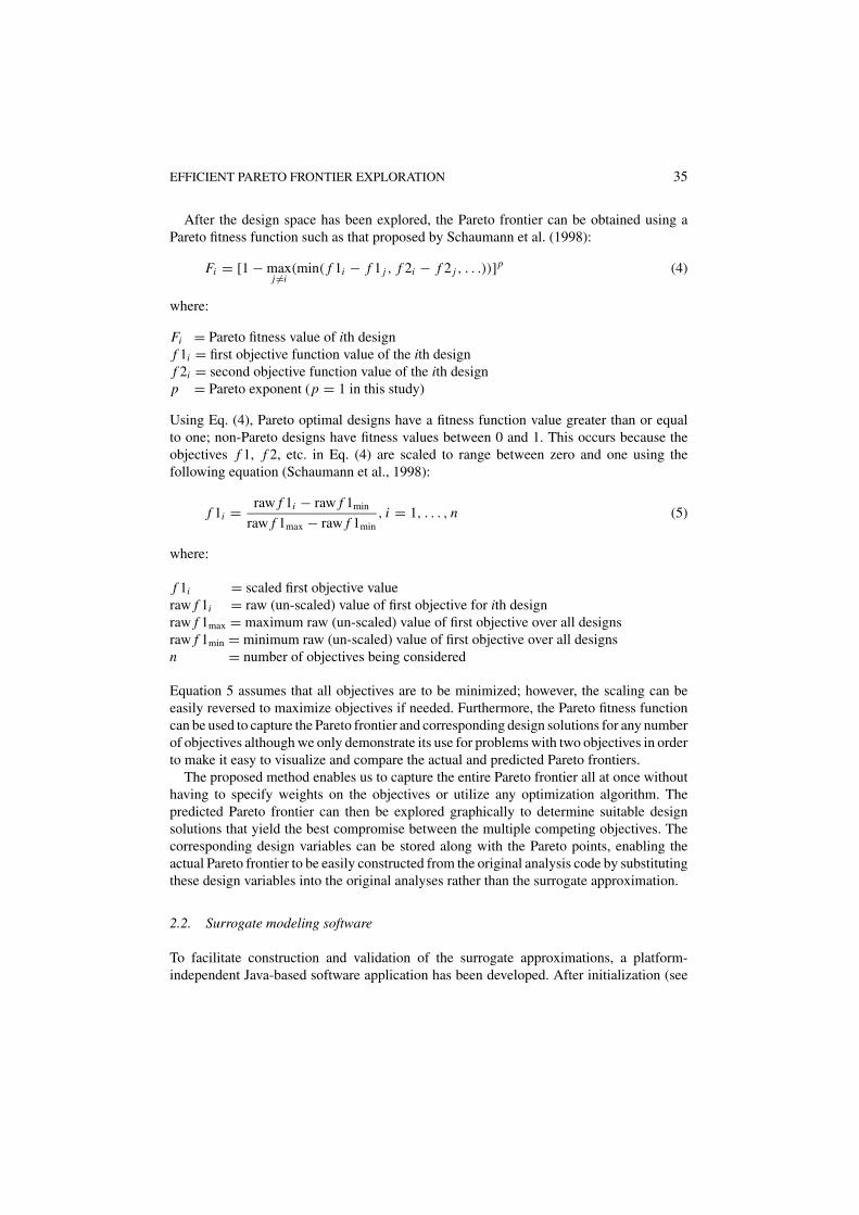
figure 2(a)), the surrogate modeling application queries the user for the design variables andtheir ranges of interest and the output responses (see figure 2(b)). The user then selects anexperimental design, and a set of data points are generated and sent to the analysis code orsimulation (see figure 2(c)). The application then constructs the selected surrogate approx-imation using the resulting sample data (see figure 2(d)) and outputs a separate Java classfile, containing the corresponding surrogate model. This Java class can then be compiledand queried as needed in place of the original analysis code. The validation tab, which isnot shown, is still under development.

To demonstrate the utility of surrogate approximations and the effectiveness of the pro-posed method for capturing the Pareto frontier, two mathematical example problems arepresented next.

3. Example problem 1

The first example is a convex, bi-criteria mathematical function with linear boundary con-straints from Li et al. (1998). The optimization problem for this example is formulated asfollows:

Minimize: f1(x1, x2) = (x1 − 2)2 + (x2 − 1)2

f2(x1, x2) = x21 + (x2 − 6)2

subject to: g1(x1, x2) = x1 − 1.6 ≤ 0(6)

g2(x1, x2) = 0.4 − x1 ≤ 0

g3(x1, x2) = x2 − 5 ≤ 0

g4(x1, x2) = 2 − x2 ≤ 0

Since the four linear constraints, g1–g4, specify the region of interest (i.e., x1 ∈ [0.4, 1.6]and x2 ∈ [2, 5]), we choose to sample only within this region to avoid infeasible solutions.Therefore, the only surrogate approximations that need to be constructed in this exampleare for f1 and f2, not the constraints.

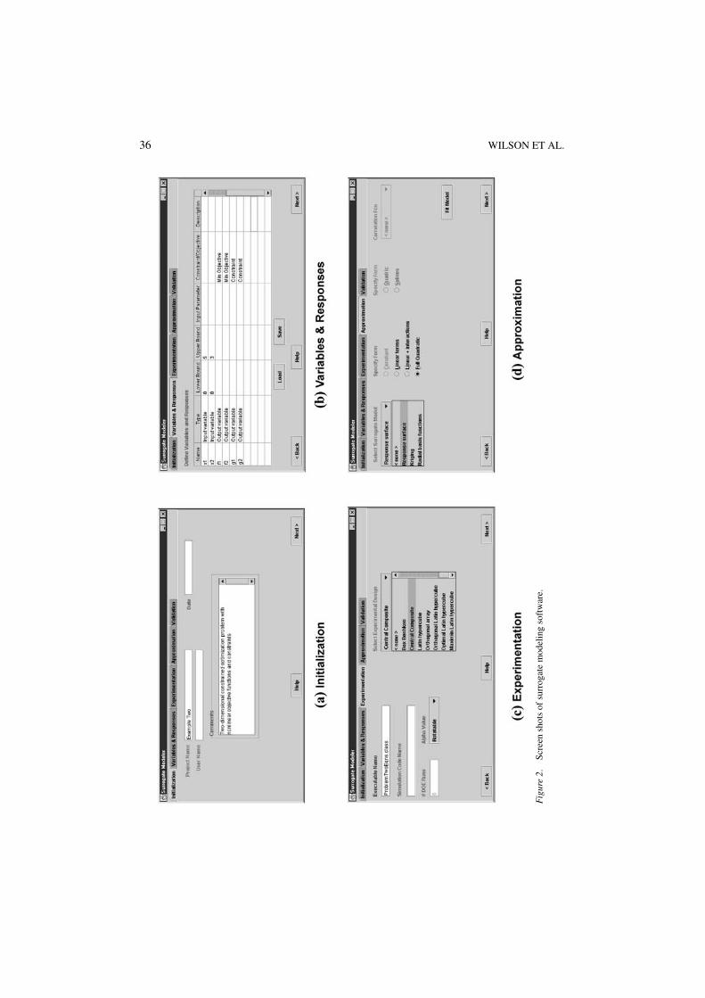
Two experimental designs are used to sample the design space: (1) a central-compositedesign (CCD) and (2) a Latin hypercube (LH); scaled versions of each design are shown infigure 3. Both designs contain nine points to ensure a fair comparison between the resultingapproximations.

The actual values of f1 and f2 at each sample point are recorded, and the resulting set ofsample data is used to construct second-order response surface models and kriging modelsfor each objective for each sample set. These surrogate models are then used to predict theresponses at a set of new design points; we sample over 10,000 points from a 101 × 101grid to generate the Pareto frontier using the Pareto fitness function in Eq. (4). The resultingPareto frontiers obtained using the response surface models and the kriging models areshown in figures 4(a) and (b), respectively. Since this example consists of two convex,second-order polynomial functions, the second-order polynomial response surface modelspredict the Pareto frontier exactly for both experimental designs.

38 WILSON ET AL.

Figure 3. Experimental designs for examples 1 and 2.

While the polynomial response surface models approximate f1 and f2 exactly, erroranalysis using maximum percent error, average percent error, and R2, is performed onthe kriging model for validation of the Pareto frontier predictions. Rather than use anadditional set of validation points to verify the kriging models, the predicted Pareto fron-tier is compared directly with the actual Pareto frontier since the actual frontier can beeasily obtained for this example over the search grid. The results of this analysis arelisted in Table 1 and are obtained by comparing the values of f1 and f2 along the actualPareto frontier with the corresponding predicted values of f1 and f2 based on the krigingmodels.

With the exception of the maximum percent error for f1, the errors listed in Table 1 arevery small, indicating that the kriging models—using only a constant term and a Gaussiancorrelation function—are nearly as accurate as second-order polynomial response surfaces.Also note that the kriging models based on the Latin hypercubes are much more accuratethan those based on the central composite design, particularly in terms of maximum percenterror. However, the R2 values for all four approximations are almost 1, indicating accuratepredictions along the Pareto frontier as seen in figure 4(b).

Table 1. Validation of kriging Pareto frontiers.

Kriging with central Kriging withcomposite design Latin hypercube

Error measure f1 f2 f1 f2

MAE (%) 22.024 6.531 0.552 0.128

AAE (%) 5.414 1.611 0.030 0.015

R2 0.9972 0.9997 0.9999 0.9999


Figure 4. Predicted Pareto frontiers for example 1.

4. Example problem 2

Our second example is a two-dimensional problem with non-linear objectives and con-straints from Tappeta and Renaud (1999a). The problem definition is as follows.

Minimize: f1(x1, x2) = (x1 + x2 − 7.5)2 + (x2 − x1 + 3)2/4

f2(x1, x2) = (x1 − 1)2/4 + (x2 − 4)2/2(7)

subject to: g1(x1, x2) = 2.5 − (x1 − 2)3/2 − x2 ≥ 0

g2(x1, x2) = 3.85 + 8(x2 − x1 + 0.65)2 − x2 − x1 ≥ 0

40 WILSON ET AL.

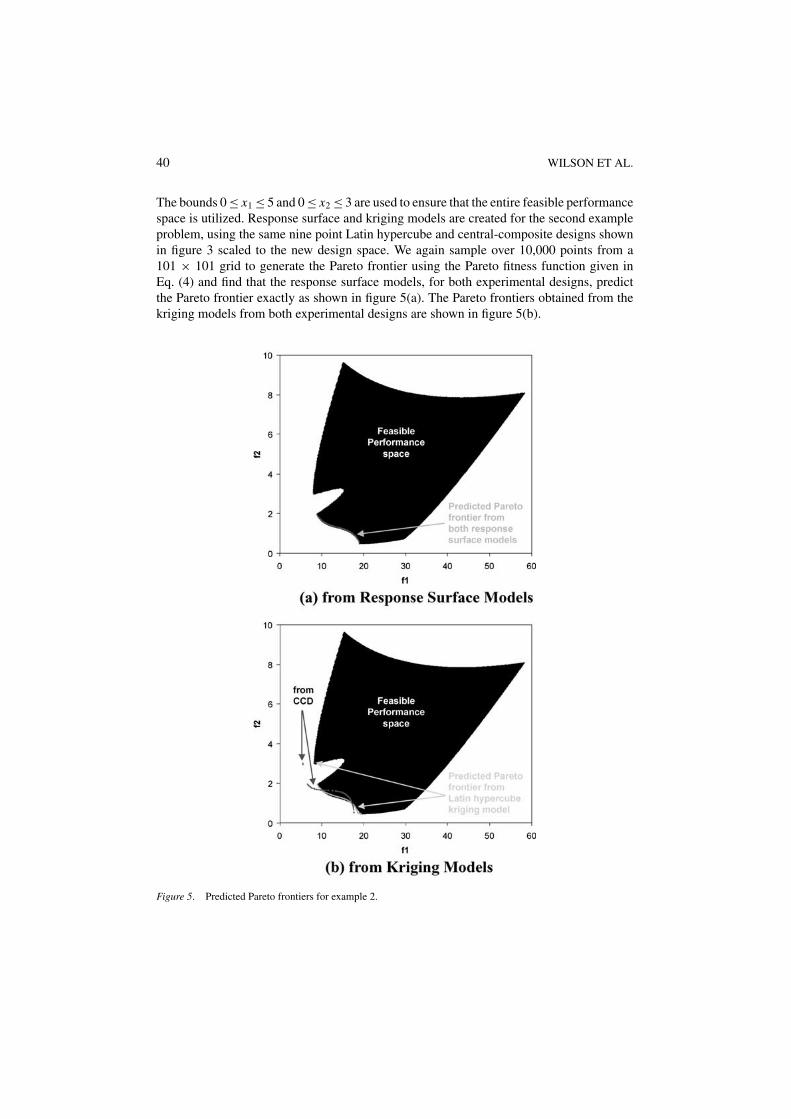
The bounds 0 ≤ x1 ≤ 5 and 0 ≤ x2 ≤ 3 are used to ensure that the entire feasible performancespace is utilized. Response surface and kriging models are created for the second exampleproblem, using the same nine point Latin hypercube and central-composite designs shownin figure 3 scaled to the new design space. We again sample over 10,000 points from a101 × 101 grid to generate the Pareto frontier using the Pareto fitness function given inEq. (4) and find that the response surface models, for both experimental designs, predictthe Pareto frontier exactly as shown in figure 5(a). The Pareto frontiers obtained from thekriging models from both experimental designs are shown in figure 5(b).

Figure 5. Predicted Pareto frontiers for example 2.


Table 2. Validation of kriging Pareto frontiers.

Kriging with central Kriging withcomposite design Latin hypercube

Error measure f1 f2 f1 f2

MAE (%) 31.741 44.421 0.074 40.135

AAE (%) 16.080 19.568 0.057 21.545

R2 0.7449 0.8070 0.9999 0.8926

As seen in figure 5(b), the kriging models created using the Latin hypercube designpredict the Pareto frontier quite accurately, but the kriging models created using the centralcomposite design do not. Error measurements for f1 and f2 for the points along the Paretofrontier for both sets of kriging models are listed in Table 2. As in Section 3, these errormeasures are computed by comparing points along the actual Pareto frontier with pointsalong the predicted Pareto frontier since it is easy to obtain the actual frontier for thisexample. These error measures are percentage errors expressed relative to the actual valuesof f1 and f2 along the true Pareto frontier. Error estimates for g1 and g2 are not computedsince relative errors measured along the Pareto frontier will be very large because g1 andg2 are zero along the frontier.

Based on this data, we note that neither kriging model predicts f2 well along the frontier;however, the kriging model based on the Latin hypercube does accurately predict f1. The R2

values for f1 and f2 for the kriging models based on the central composite design are poor,and the maximum percent error and average percent error are also quite large. Despite thelarge maximum percent error and average percent error for f2 for the kriging models basedon the Latin hypercube, the R2 values for f1 and f2 are acceptable for an approximation.So while none of the kriging models predict as well as they did in the first example, thekriging models based on the Latin hypercube are more accurate than those based on thecentral composite design.

One explanation for the discrepancy between the performance of the two designs resultsfrom an interaction between the kriging model and the experimental design type. Due to thelocation and spacing of the sample points in the design space in a central composite design,the correlation matrix based on the Gaussian correlation function in the fitted kriging modeltends to be singular or near singular when maximum likelihood estimation is performed toobtain the theta parameters used to fit the model. To confirm this, the condition numbersof the correlation matrices for each response for each design are listed in Table 3. Wehave found that a condition number smaller than 10−12 indicates that significant round-off error can occur during prediction because the correlation matrix is close to singular.Such is the case for the kriging models for f1 and f2 based on the central compositedesign.

Despite the slight approximation error in the kriging models, the Pareto points themselves(i.e., the design variables x1 and x2 corresponding to each point on the Pareto frontier) arenearly identical to the actual Pareto points obtained from the original set of equations asseen in figure 6. Figure 6(a) shows the Pareto points obtained from the response surface

42 WILSON ET AL.

Table 3. Condition numbers of kriging model correlation matrices.

Condition Kriging with central Kriging withnumber composite design Latin hypercube

f1 2.8821D-15 1.2165D-09

f2 1.3950D-14 8.5201D-10

g1 1.0345D-08 2.2178D-09

g2 6.4121D-13 2.2982D-06

Figure 6. Mapping the design space of the Pareto frontier for example 2.

models overlaying the actual Pareto points; those obtained from the kriging models basedon the Latin hypercube design are shown in figure 6(b).

While considerable error exists in the Pareto frontier obtained using the kriging modelsbased on the central composite design, the kriging models based on the Latin hypercubedesign and both sets of response surface models are able to capture the Pareto frontieraccurately. In this case, the Pareto frontier is successfully captured without the use of opti-mization even though it is non-convex and discontinuous. This example also demonstratesthe importance of validating the surrogate approximations to ensure that they are sufficientlyaccurate before attempting to capture the Pareto frontier; otherwise, the predicted and actualfrontiers may be vastly different.

5. Design of a piezoelectric bimorph actuator

Our final example comes from current research work in which we are trying to simultane-ously optimize the maximum deflection and blocked force of a piezoelectric bimorph actu-ator for minimally invasive surgery (Cappelleri and Frecker, 1999; Cappelleri et al., 1999,2001). A piezoelectric bimorph actuator is created by laminating layers of piezoelectric


Figure 7. Bimorph actuator (Fatikow and Rembold, 1997).

Figure 8. A piezoelectric bimorph grasper.

ceramic material (PZT) onto a thin sandwich beam or plate. When opposing voltages areapplied to the two ceramic layers, a bending moment is induced in the beam, see figure 7.A pair of cantilevered piezoelectric bimorph actuators can be used as a simple graspingdevice, where the bimorph actuators are used as active “fingers” as shown in figure 8.

The objective in this example is to design a PZT bimorph grasper for application inminimally invasive surgical procedures. The performance of the PZT bimorph actuator isevaluated in terms of the tip force and deflection: a large tip deflection is required so thatthe jaws of the grasper can close completely, and a large tip force is required to securelygrasp a suture needle and prevent it from rolling in the jaws. These performance criteriaare determined by the thickness and width of each PZT layer, the length of the actuator, thematerial properties, and the applied voltage. The force available at the tip is modeled as theblocked force (i.e., the force exerted with no deflection), and the deflection is modeled asthe free deflection. The results from preliminary analysis indicate that a standard, commer-cially available bimorph of the size required for MIS is infeasible since there is insufficientgrasping force and tip deflection (Cappelleri et al., 2001). Consequently, a variable thicknessdesign, where the thickness of the layers is varied along the length, is proposed to improvethe deflection and force performance of the PZT bimorph actuator.

The piezoelectric bimorph actuator is modeled as a composite beam with a thin steelsandwich layer and PZT5H (IEEE, 1978) top and bottom layers. Rather than allowingthe thickness of the PZT layers to vary continuously along the length, the layers are dis-cretized into five sections to allow for simple modeling, where the thickness of each section,

44 WILSON ET AL.

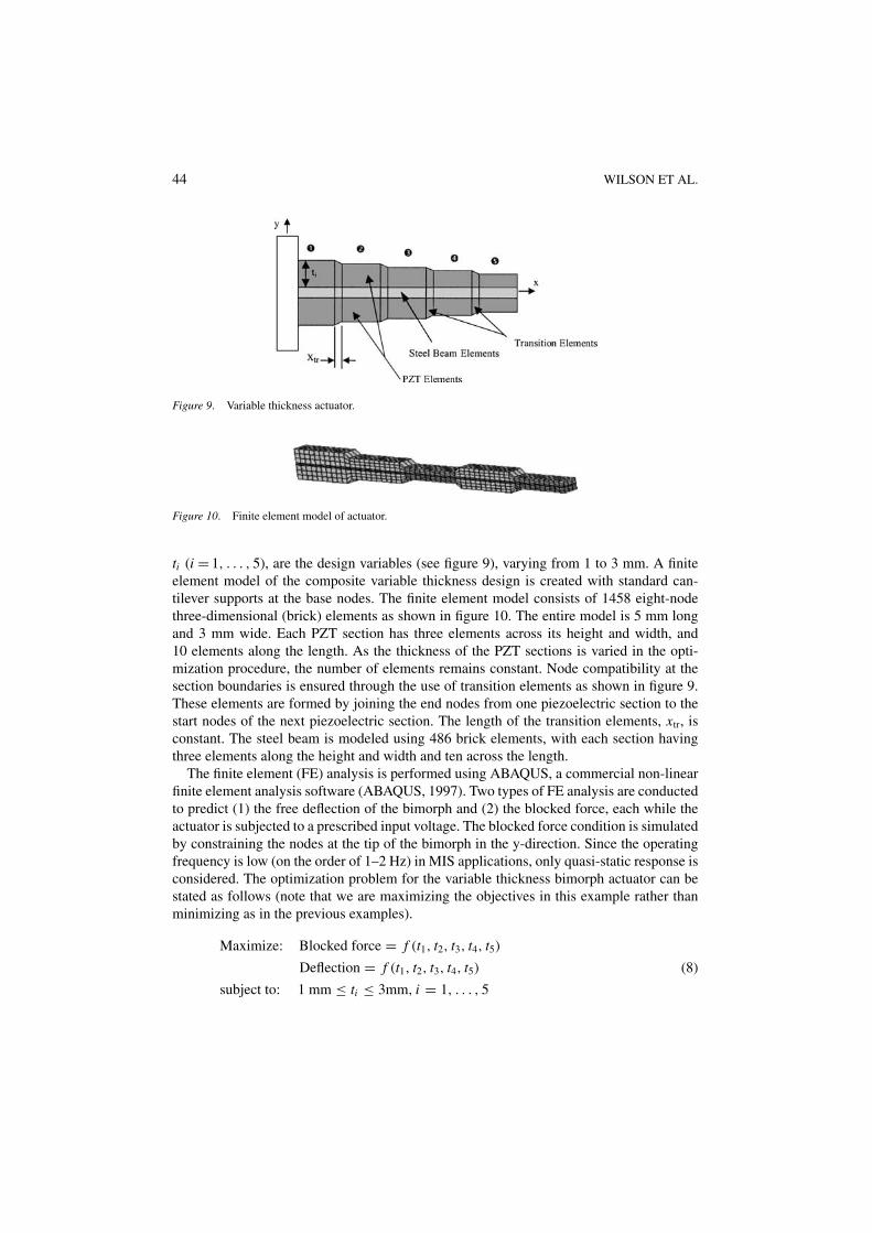
Figure 9. Variable thickness actuator.

Figure 10. Finite element model of actuator.

ti (i = 1, . . . , 5), are the design variables (see figure 9), varying from 1 to 3 mm. A finiteelement model of the composite variable thickness design is created with standard can-tilever supports at the base nodes. The finite element model consists of 1458 eight-nodethree-dimensional (brick) elements as shown in figure 10. The entire model is 5 mm longand 3 mm wide. Each PZT section has three elements across its height and width, and10 elements along the length. As the thickness of the PZT sections is varied in the opti-mization procedure, the number of elements remains constant. Node compatibility at thesection boundaries is ensured through the use of transition elements as shown in figure 9.These elements are formed by joining the end nodes from one piezoelectric section to thestart nodes of the next piezoelectric section. The length of the transition elements, xtr, isconstant. The steel beam is modeled using 486 brick elements, with each section havingthree elements along the height and width and ten across the length.

The finite element (FE) analysis is performed using ABAQUS, a commercial non-linearfinite element analysis software (ABAQUS, 1997). Two types of FE analysis are conductedto predict (1) the free deflection of the bimorph and (2) the blocked force, each while theactuator is subjected to a prescribed input voltage. The blocked force condition is simulatedby constraining the nodes at the tip of the bimorph in the y-direction. Since the operatingfrequency is low (on the order of 1–2 Hz) in MIS applications, only quasi-static response isconsidered. The optimization problem for the variable thickness bimorph actuator can bestated as follows (note that we are maximizing the objectives in this example rather thanminimizing as in the previous examples).

Maximize: Blocked force = f (t1, t2, t3, t4, t5)

Deflection = f (t1, t2, t3, t4, t5) (8)

subject to: 1 mm ≤ ti ≤ 3mm, i = 1, . . . , 5


Table 4. Validation of surrogate approximations.

Response surfaces Kriging models

Error measure Deflection Force Deflection Force

MAE (%) 13.78 18.99 18.06 8.02

AAE (%) 6.23 4.33 7.09 2.83

R2 0.953 0.766 0.999 0.999

While Latin hypercubes were found to be more effective in the previous examples, onlya face-centered central composite design (CCD) is used to sample the design space sinceit only requires three levels of the design variables to be analyzed (ti = 1 mm, 2 mm,and 3 mm). The face-centered CCD consists of 27 points: 16 points from a half-fractionResolution V factorial design, 10 “star” points, and 1 center point. Data from these 27sample points is used to construct response surface models and kriging approximations forboth blocked force and deflection. Both sets of approximations are then used in lieu of theABAQUS finite element analysis to search the design space to predict the Pareto frontier.

After constructing both sets of approximations, a set of twenty-five random points from aLatin hypercube are used to validate each set of approximations since it is too computation-ally expensive to determine the actual Pareto frontier in ABAQUS for comparison as we didin Sections 3 and 4. The maximum percent error, average percent error, and R2 values forthe response surface and kriging models for the deflection and blocked force are listed inTable 4. The error in the predicted deflection is comparable for both approximations, withthe response surface models yielding slightly lower maximum percent error and averagepercent error; however, in the case of the blocked force response, the kriging model fits thedata much more accurately. Comparison of R2 values across approximations further revealsthat the kriging models are much more accurate than the response surface models since R2

is nearly 1 for both kriging models.To understand the tradeoff between the deflection and blocked force objectives, the

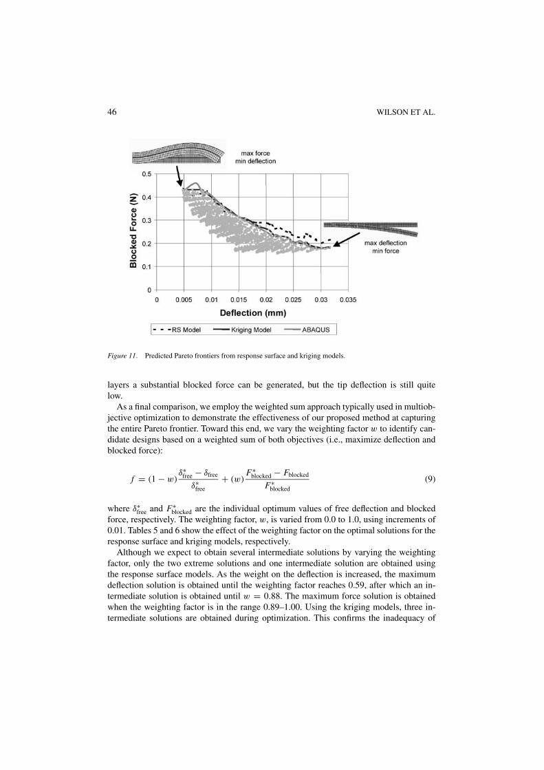
approximations are used to search the design space and find the Pareto frontier. The designspace is explored by predicting the blocked force and deflection of 3125 design pointsbased on a 55 grid that searches over all section thicknesses in 0.5 mm increments based onreadily available material sizes using the response surface models and the kriging models.The Pareto frontier is then obtained by selecting points on the boundary of the design spaceas predicted by the response surface models and the kriging models as shown in figure 11.The points on the Pareto frontier, as predicted by the response surface models and krigingmodels, are compared to one another, and the points with common thickness settings areevaluated in ABAQUS to verify the actual response. The results of this analysis are alsoshown in figure 11.

As seen in the figure, the kriging models are good predictors of the points along the Paretofrontier, while the response surface models are not for points that have a large deflectionand small blocked force. This result is consistent with the data in Table 4 as the responsesurface model is generally less accurate than the kriging model based on the set of validationpoints. It is also evident from figure 11 that by varying the thickness of the piezoelectric

46 WILSON ET AL.

Figure 11. Predicted Pareto frontiers from response surface and kriging models.

layers a substantial blocked force can be generated, but the tip deflection is still quitelow.

As a final comparison, we employ the weighted sum approach typically used in multiob-jective optimization to demonstrate the effectiveness of our proposed method at capturingthe entire Pareto frontier. Toward this end, we vary the weighting factor w to identify can-didate designs based on a weighted sum of both objectives (i.e., maximize deflection andblocked force):

f = (1 − w)δ∗

free − δfree

δ∗free

+ (w)F∗

blocked − Fblocked

F∗blocked

(9)

where δ∗free and F∗

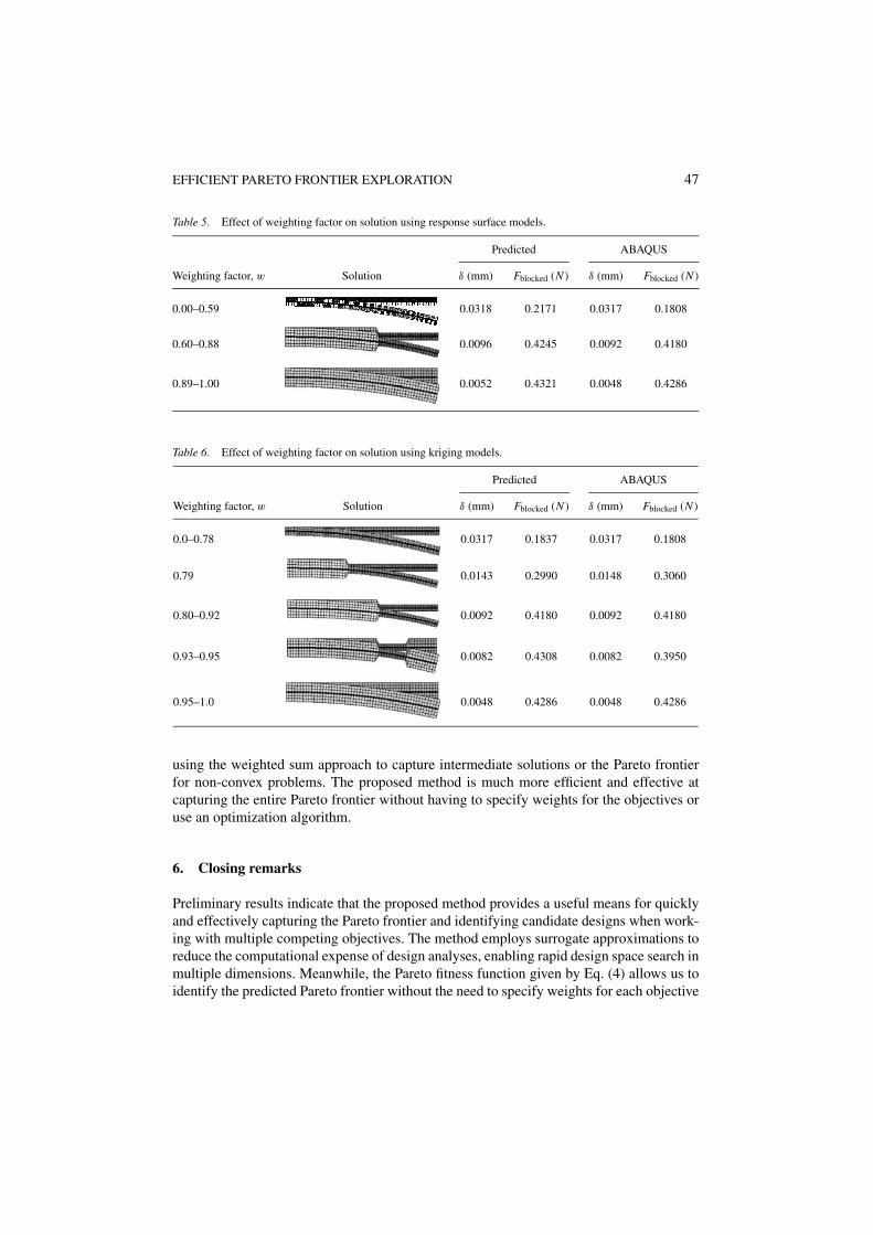
blocked are the individual optimum values of free deflection and blockedforce, respectively. The weighting factor, w, is varied from 0.0 to 1.0, using increments of0.01. Tables 5 and 6 show the effect of the weighting factor on the optimal solutions for theresponse surface and kriging models, respectively.

Although we expect to obtain several intermediate solutions by varying the weightingfactor, only the two extreme solutions and one intermediate solution are obtained usingthe response surface models. As the weight on the deflection is increased, the maximumdeflection solution is obtained until the weighting factor reaches 0.59, after which an in-termediate solution is obtained until w = 0.88. The maximum force solution is obtainedwhen the weighting factor is in the range 0.89–1.00. Using the kriging models, three in-termediate solutions are obtained during optimization. This confirms the inadequacy of


Table 5. Effect of weighting factor on solution using response surface models.

Predicted ABAQUS

Weighting factor, w Solution δ (mm) Fblocked (N ) δ (mm) Fblocked (N )

0.00–0.59 0.0318 0.2171 0.0317 0.1808

0.60–0.88 0.0096 0.4245 0.0092 0.4180

0.89–1.00 0.0052 0.4321 0.0048 0.4286

Table 6. Effect of weighting factor on solution using kriging models.

Predicted ABAQUS

Weighting factor, w Solution δ (mm) Fblocked (N ) δ (mm) Fblocked (N )

0.0–0.78 0.0317 0.1837 0.0317 0.1808

0.79 0.0143 0.2990 0.0148 0.3060

0.80–0.92 0.0092 0.4180 0.0092 0.4180

0.93–0.95 0.0082 0.4308 0.0082 0.3950

0.95–1.0 0.0048 0.4286 0.0048 0.4286

using the weighted sum approach to capture intermediate solutions or the Pareto frontierfor non-convex problems. The proposed method is much more efficient and effective atcapturing the entire Pareto frontier without having to specify weights for the objectives oruse an optimization algorithm.

6. Closing remarks

Preliminary results indicate that the proposed method provides a useful means for quicklyand effectively capturing the Pareto frontier and identifying candidate designs when work-ing with multiple competing objectives. The method employs surrogate approximations toreduce the computational expense of design analyses, enabling rapid design space search inmultiple dimensions. Meanwhile, the Pareto fitness function given by Eq. (4) allows us toidentify the predicted Pareto frontier without the need to specify weights for each objective

48 WILSON ET AL.

function or use any optimization. The predicted Pareto frontier can then be verified usingthe original analyses to estimate the actual Pareto frontier. The method works well for bothconvex and non-convex Pareto frontiers, even when discontinuities are present, as demon-strated in Section 3 and 4. We note that it is important that the surrogate approximationsare validated and sufficiently accurate; otherwise, the predicted Pareto frontier will be in-accurate. The example problem in Section 4 demonstrated how inaccurate approximationscan yield poor predictions along the Pareto frontier. If achieving accurate surrogate approx-imations is difficult, alternative metamodel types or experimental design strategies couldbe employed in an effort to improve modeling accuracy. This has been demonstrated bycomparing results from two types of experimental designs (i.e., central composite designsand Latin hypercubes) and two types of surrogate approximations (i.e., response surfacesand kriging models) in each example problem. The method is very flexible and can easilyaccommodate a wide variety of experimental designs and approximations.

While three examples do not completely validate the method itself, the results to dateare promising. While the examples contained herein are for multicriteria problems withtwo objectives, we do not anticipate any problems adapting our method to multicriteriaproblems with more than two objectives. The Pareto fitness function in Eq. (4) easily scalesto higher dimensions; however, visualizing more than two objectives at once remains achallenge. The proposed method also does not restrict the use of an optimization algorithmto facilitate the search for the Pareto frontier using the surrogate models; however, we dowish to avoid having to specify weights a priori for each objective. We envision that a geneticalgorithm-based approach such as that proposed in (Azarm et al., 1999; Balling et al., 1999;Schaumann et al., 1998) could greatly facilitate the design space search; however, we havenot yet implemented such an approach.

Acknowledgments

We appreciate the helpful comments and suggestions from our reviewers. The work byBenjamin Wilson and Dr. Simpson was supported by Dr. Kam Ng, ONR 333, through theNaval Sea Systems Command under Contract No. N00039-97-D-0042 and N00014-00-G-0058. The work by David Cappelleri and Dr. Frecker was supported by the Charles E.Culpeper Foundation Biomedical Pilot Initiative.

References

ABAQUS Version 5.7-1, Hibbitt, Karlsson and Sorensen, Inc., 1080 Main Street, Pawtucket, RI, (URL:http://www.hks.com/), 1997.

T. W. Athan and P. Y. Papalambros, “A note on weighted criteria methods for compromise solutions in multi-objective optimization,” Engineering Optimization vol. 27, no. 2, pp. 155–176, 1996.

S. Azarm, B. J. Reynolds, and S. Narajanan, “Comparison of two multiobjective optimization techniques with andwithin genetic algorithms,” Advances in Design Automation, Las Vegas, NV, ASME, Sept. 12–15, 1999, PaperNo. DETC99/DAC-8584.

R. Balling, “Design by shopping: A new paradigm?,” Proc. Third World Congress of Structural and Multidisci-plinary Optimization, C. L. Bloebaum and K. E. Lewis et al., eds. Buffalo, NY, University at Buffalo vol. 1,May 17–21, 1999, pp. 295–297.


R. J. Balling, J. T. Taber, M. R. Brown, and K. Day, “Multiobjective urban planning using genetic algorithm,”Journal of Urban Planning and Development vol. 125, no. 2, pp. 86–99, 1999.

J.-F. M. Barthelemy and R. T. Haftka, “Approximation concepts for optimum structural design—A review,”Structural Optimization vol. 5, pp. 129–144, 1993.

A. J. Booker, “Design and analysis of computer experiments,” 7th AIAA/USAF/NASA/ISSMO Symposium onMultidisciplinary Analysis & Optimization, St. Louis, MO, AIAA vol. 1, Sept. 2–4, 1998, pp. 118–128. AIAA-98-4757.

D. J. Cappelleri and M. I. Frecker, “Optimal design of smart tools for minimally invasive surgery,” Optimizationin Industry II, F. Mistree and A. D. Belegundu, eds. Banff, Alberta, Canada, ASME, July 6–11, 1999.

D. J. Cappelleri, M. I. Frecker, and T. W. Simpson, “Optimal design of a PZT bimorph actuator for minimallyinvasive surgery,” 7th International Symposium on Smart Structures and Materials, Newport Beach, CA, SPIE,Mar. 5–9, 1999.

D. J. Cappelleri, M. I. Frecker, T. W. Simpson, and A. Snyder, “A metamodel-based approach for optimal designof a PZT bimorph actuator for minimally invasive surgery,” Journal of Mechanical Design 2001, to appear.

F. Y. Cheng and D. Li, “Multiobjective optimization design with Pareto genetic algorithm,” Journal of StructuralEngineering vol. 123, no. 9, pp. 1252–1261, 1997.

I. Das, “An improved technique for choosing parameters for Pareto surface generation using normal-boundaryintersection,” Proc. Third World Congress of Structural and Multidisciplinary Optimization (WCSMO-3) C. L.Bloebaum and K. E. Lewis et al., eds., Buffalo, NY, University at Buffalo, vol. 2, May 17–21, 1999, pp. 411–413.

I. Das, “Optimization large systems via optimal multicriteria component assembly,” 7th AIAA/USAF/NASA/ISSMOSymposium on Multidisciplinary Analysis & Optimization, St. Louis, MO, AIAA, vol. 1, Sept. 2–4, 1998,pp. 661–669, AIAA-98-4791.

I. Das and J. E. Dennis, “A closer look at drawbacks of minimizing weighted sums of objectives for Paretoset generation in multicriteria optimization problems,” Structural Optimization vol. 14, no. 1, pp. 63–69,1997.

I. Das, and J. E. Dennis, “Normal-boundary intersection: A new method for generating the Pareto surface innonlinear multicriteria optimization problems,” SIAM Journal on Optimization vol. 8, no. 3, pp. 631–657, 1998.

W. Fatikow and Rembold, U., Microsystem Technology and Microrobotics, Springer-Verlag: New York, 1997.A. Giunta, L. T. Watson, and J. Koehler, “A comparison of approximation modeling techniques: Polynomial versus

interpolating models,” 7th AIAA/USAF/NASA/ISSMO Symposium on Multidisciplinary Analysis & Optimization,St. Louis, MO, AIAA vol. 1, Sept. 2–4, 1998, pp. 392–404. AIAA-98-4758.

IEEE Group on Sonics and Ultrasonics, Transducers and Resonators Committee, IEEE Standard on Piezoelectricity(176-1978), ANSI/IEEE: New York, 1978.

E. M. Kasprazak and K. E. Lewis, “A method to determine optimal relative weights for Pareto solution sets,” Proc.Third World Congress of Structural and Multidisciplinary Optimization (WCSMO-3), C. L. Bloebaum andK. E. Lewis et al., eds., Buffalo, NY, University at Buffalo vol. 2, May 17–21, 1999, pp. 408–410.

J. R. Koehler and A. B. Owen, “Computer experiments,” Handbook of Statistics, S. Ghosh and C. R. Rao, eds.Elsevier Science: New York, 1996, pp. 261–308.

J. Koski, “Defectiveness of weighting method in multicriterion optimization of structures,” Communications inApplied Numerical Methods vol. 1, pp. 333–337, 1985.

Y. Li, G. M. Fadel, and M. M. Wiecek, “Approximating Pareto curves using the hyper-ellipse,” 7thAIAA/USAF/NASA/ISSMO Symposium on Multidisciplinary Analysis & Optimization, St. Louis, MO, AIAAvol. 3, Sept. 2–4, 1998, pp. 1990–2002.

E. R. Liberman, “Soviet multi-objective mathematical programming methods: An overview,” Management Sciencevol. 37, no. 9, pp. 1147–1165, 1991.

M. D. McKay, R. J. Beckman, and W. J. Conover, “A comparison of three methods for selecting values of inputvariables in the analysis of output from a computer code,” Technometrics vol. 21, no. 2, pp. 239–245, 1979.

M. Meckesheimer, R. R. Barton, T. W. Simpson, and A. Booker, “Computationally inexpensive metamodel assess-ment strategies,” ASME Design Technical Conferences—Design Automation Conference A. Diaz, ed. Pittsburgh,PA, ASME, Sept. 9–12, 2001, DETC2001/DAC-21028.

A. Messac, J. G. Sundararaj, R. V. Tappeta, and J. E. Renaud, “The ability of objective functions to gener-ate non-convex Pareto frontiers,” 40th AIAA/ASME/ASCE/AHS/ASC Structures, Structural Dynamics, and

50 WILSON ET AL.

Materials Conference and Exhibit, St. Louis, MO, AIAA vol. 1, Apr. 12–15, 1999, pp. 78–87. AIAA-99-1211.

R. H. Myers, and D. C. Montgomery, Response Surface Methodology: Process and Product Optimization UsingDesigned Experiments, John Wiley & Sons: New York, 1995.

A. Osyczka, “Multicriteria optimization for engineering design,” in Design Optimization, J. S. Gero, ed. AcademicPress: New York, 1985, pp. 193–227.

A. Osyczka and S. Kundu, “A new method to solve generalized multicriteria optimization problems using thesimple genetic alrogithm,” Structural Optimization vol. 10, no. 2, pp. 94–99, 1995.

A. B. Owen, “Orthogonal arrays for computer experiments, integration and visualization,” Statistica Sinicavol. 2, pp. 439–452, 1992.

J. Sacks, W. J. Welch, T. J. Mitchell, and H. P. Wynn, “Design and analysis of computer experiments,” StatisticalScience vol. 4, no. 4, pp. 409–435, 1989.

E. J. Schaumann, R. J. Balling, and K. Day, “Genetic algorithms with multiple objectives,” 7thAIAA/USAF/NASA/ISSMO Symposium on Multidisciplinary Analysis & Optimization, St. Louis, MO, AIAAvol. 3, Sept. 2–4, 1998, pp. 2114–2123.

T. W. Simpson, T. M. Mauery, J. J. Korte, and F. Mistree. “Comparison of response surface and kriging modelsfor multidisciplinary design optimization,” 7th AIAA/USAF/NASA/ISSMO Symposium on MultidisciplinaryAnalysis & Optimization, St. Louis, MO, AIAA vol. 1, Sept. 2–4, 1998, pp. 381–391, AIAA-98-4755.

T. W. Simpson, T. M. Mauery, J. J. Korte, and F. Mistree, “Kriging metamodels for global approximation insimulation-based multidisciplinary design optimization,” AIAA Journal 2001, to appear.

T. W. Simpson, J. Peplinski, P. N. Koch, and J. K. Allen, “Metamodels for computer-based engineering design:Survey and recommendations,” Engineering with Computers vol. 17, pp. 129–150, 2001.

J. Sobieszczanski-Sobieski and R. T. Haftka, “Multidisciplinary aerospace design optimization: Survey of recentdevelopments,” Structural Optimization vol. 14, pp. 1–23, 1997.

I. M. Sobol, “An efficient approach to multicriteria optimum design problems,” Surveys on Mathematics forIndustry vol. 1, pp. 259–281, 1992.

W. Stadler and J. Dauer, “Multicriteria optimization in engineering: A tutorial and survey,” Structural Optimization:Status and Promise, M. P. Kamat, ed., AIAA: Washington, D.C., 1993, pp. 209–249.

R. E. Steuer, Multiple Criteria Optimization: Theory, Computation, and Application, Wiley: New York, 1986.R. V. Tappeta and J. E. Renaud, “Interactive multiobjective optimization design strategy for decision based

design,” Advances in Design Automation, Las Vegas, NV, ASME, Sept. 12–15, 1999a, Paper No. DETC99/DAC-8581.

R. V. Tappeta, and J. E. Renaud, “Interactive multiobjective optimization procedure,” 40th AIAA/ASME/ASCE/AHS/ASC Structures, Structural Dynamics, and Materials Conference and Exhibit, St. Louis, MO, AIAAvol. 1, Apr. 12–15, 1999b, pp. 27–41, AIAA-99-1207.

R. V. Tappeta, J. E. Renaud, A. Messac, and J. G. Sundararaj, “Interactive physical programming: Tradeoff analysisand decision making in multicriteria optimization,” 40th AIAA/ASME/ASCE/AHS/ASC Structures, StructuralDynamics, and Materials Conference and Exhibit, St. Louis, MO, AIAA vol. 1, Apr. 12–15, 1999, pp. 53–67,AIAA-99-1209.

J. Zhang, M. M. Wiecek, and W. Chen, “Local approximation of the efficient frontier in robust design,” Advancesin Design Automation, Las Vegas, NV, ASME, Sept. 12–15, 1999, Paper No. DETC99/DAC-8566.

Documents

Efficient Pareto Frontier Exploration using Surrogate Approximations