Embed Size (px)
Citation preview
Effect of Dynamic Interaction between Train Vehicle and Structure on Seismic Response of Structure Munemasa TOKUNAGA & Masamichi SOGABE Railway Technical Research Institute, Japan
SUMMARY: The conventional seismic standard specifies that the seismic inertia force of trains is modelled as the rigid mass which has the upper limit force of 30% of the train weight on insufficient grounds. However, train actions on railway structures during earthquakes have not been identified, although actual train vehicles are the complicated vibration system. The object of this paper is to quantify dynamic interactions between train vehicles and structures during earthquakes, and to develop a reasonable train action model. Numerical simulations clarified that the dynamic interaction consisting on the creep force and the contact force between wheels and rails changes depending on response level. Additionally, the displacement response of heavy structures, such as RC structures can be evaluated without considering the effect of the dynamic interaction, and that of light structures, such as steel bridges of open floor type, should be evaluated with considering the effect of the dynamic interaction. Keywords: Dynamic interaction, Train vehicle, railway structure, non-linear analysis, Seismic design 1. INTRODUCTION Lots of old railway steel bridges, which are of open floor type without concrete slabs, are light weight bridges of unit weight/length of 30 kN/m. From a view point of the seismic design or the seismic diagnosis of these bridges, the percentage of the train weight, which is assumed to be approximate 35 kN/m, to the entire bridge weight is high. Therefore, seismic response of these light bridges may be significantly affected by train behaviour and train actions on the bridges. The Design Standards for Railway Structures and Commentary established by RTRI (Seismic Design) (hereinafter referred to as the seismic standard) (RTRI, 1999) specifies that the seismic inertia force of trains is loaded as an uniformly-distributed fixed load on the condition of riding capacity of 100% (70% for a freight car). The frequencies of trains determine the number of track where trains load is loaded. The seismic inertia force has the upper limit value of 30% of the train weight assuming that train vehicles have some damping effects or do not always oscillate in the same phase as structures. This upper limit value can be used at need. An Example of Seismic Verification for a RC Railway Rigid-Frame Viaduct (RTRI, 2008) presents the calculation method for seismic responses based on the static analysis. In this method, the seismic coefficient and the equivalent natural period are obtained from the static pushover analysis under the condition of 30% of the train weight included in the weight of structures, and the displacement response during design earthquake motion is calculated using the non-linear spectrum method. This method gives calculation results under the same conditions as the dynamic response analysis based on the dynamic characteristics in the case where the train weight is assumed to be light. A Guideline of Seismic Verification (RTRI, 2006) explains the method where the train action is assumed to be SDOF system in the dynamic analysis. The spring of SDOF system is modeled as a
bi-linear type spring where rigidity is well strong before the yield point and much less string after the point. The yield force of the spring is set at 30% of the train weight which is the upper limit value of the seismic inertia force. On the other hand, sufficient reason why the upper limit of the inertia force is 30% of the train weight in these methods has not been clarified sufficiently, and neither such train modeling ways for train actions during earthquakes has been verified. The actual train vehicle is the complicated vibration system consisting of a carbody, two truck frames, four wheelsets, some springs, dampers and stoppers. Actions to railway structures which can be caused by the train vehicles during earthquakes have not been identified. In addition, in recent years, measures against derailment such as anti-derailing guard rail have been established, which will bring about greater dynamic interactions between train vehicles and railway structures when huge earthquakes happen. Therefore, it is necessary to investigate more reasonable modeling methods for train seismic actions. The object of this paper is to quantify dynamic interactions between train vehicles and railway structures during earthquakes, and to develop reasonable train action models through the following investigations. (1) To clarify mechanisms of dynamic interactions between train vehicles and railway structures
during earthquakes. (2) To clarify effect of dynamic interactions on dynamic characteristics of structures. (3) To discuss reasonable train models for estimating displacement response of railway structures
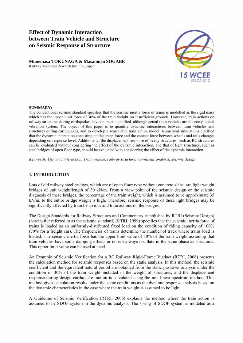
during earthquake. 2. ANALYSIS METHOD A program called DIASTARSIII, which analyses dynamic interaction between vehicles and railway structures, was used in the numerical analysis (Wakui, H., et al., 1994). 2.1. Dynamic Model of Structure Fig. 1 (a) shows the dynamic model of structures. The dynamic behaviour of railway structures can be often expressed by the single degree of freedom (SDOF). Therefore, structures were modelled as SDOF system with the tri-linear type skeleton curve and the standard type hysteric characters. For the skeleton curve, the yield seismic coefficient khy, the maximum seismic intensity khmax, the equivalent natural period Teq, and the structure unit weight/length ws, were set as the parameters. The second gradient was set to 1/10 of the first gradient and the third gradient was set to infinitesimal. The equivalent natural period of structures was calculated on the basis of structure weight of 100% and train weight of 100% in the each train modelling way. The structure weight is set in consideration of 25 m which is the same length as the train vehicle.
Large mass
Rigid beam: Uniformly-distributed mass
M
Interaction forces
Train vehicle: Multi body system (1-car train, 260km/h)
Accelaration input
Spring of structure
Detailed model Simplified model
M
Structure mass
Train massStructure
Displacement δ
Seismic coefficient
←ω02=K/m
←ω02/10
Non-Linear spring of structure
Hysteric character: Standard type
khmax
khy
Equivalent natural period
(a) Dynamic model of structure(b) Dynamic model of train vehicle and dynamic interaction between train vehicle and railway structure
Figure 1 Dynamic model of structure and dynamic interaction between train vehicle and structure
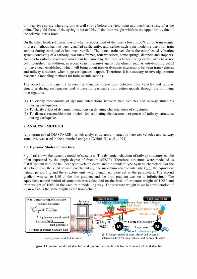
2.2. Dynamic Model of Train Vehicles and Dynamic Interaction between Wheels and Rails Fig. 1 (b) indicates conceptual diagrams of modelling way of train vehicles and dynamic interactions between train vehicles and structures, the detailed model and the simplified model. 2.2.1. Detailed model Fig. 2 shows the dynamic model of train vehicles of the detailed model. The train vehicle model was created by connecting element of a carbody, 2 truck frames and 4 wheelsets which were modelled at rigid bodies with springs and dampers. Then, a train vehicle has 31degrees of freedom. Actual vehicles have stoppers to control excessive relative displacements at each connection. In order to consider the stoppers, bi-linear springs were used for springs. Adequacy of these dynamic models has already been verified through vibration experiments using a vibration table and a full-scale vehicle model (Miyamoto, T, et al., 2007). Tangible vehicle specifications were assumable in reference to a recent high-speed Shinkansen train vehicle. The main input data of the mass are a vehicle length of 25mf, a carbody mass of 312kN, a truck frame mass of 31kN, a wheelset mass of 18kN for an empty vehicle, therefore, the weight of a train vehicle is 446kN and the unit weight/length of train vehicle investigated in this study is 17.8 kN/m. The main input data of springs and dampers are vertical and horizontal spring constants for air-spring of 300kN/m and 180kN/m (half side of a truck), a damping constant for air-spring of 50kN・s/m (half side of a truck), a damping constant for lateral damper of 40kNs/m (a damper of a truck), 1200kN/m of the spring constant for axle spring (half side of a wheelset) and the damping constant for axle damper of 40 kNs/m (half side of a wheelset). In addition, gaps at each stopper were set to be 20-30mm. We conducted simulates under the condition that 1-car train, which keep running at 260km/h, interacts with structures without the derailment and the deviation. This condition is supposed to be most severe for seismic response of structures. Fig. 3 shows dynamic interactions between wheels and rails of the detailed model. Dynamic interaction forces between wheels and rails were calculated on the basis of vertical and horizontal relative displacements between wheels and rails. The dynamic interaction force of vertical direction is modelled as the Hertz contact force and that of horizontal direction is modelled as the creep force and the flange pressure. The Hertz contact force is the vertical force which is the function of the vertical relative displacement between the wheel and the rail δz. The creep force is the horizontal force which is caused by the creep of the wheel moving forward by rolling on the rail. This creep force is saturated
zψ φ
Wheelset
Carbody ψ θz
y
ψT
zT
yTθT
θW
zW
Air springzTψT
φT
zW ψWφW
ψW yW
K3, C3
Kwz, Cwz
Coupler
Rigid Body
Axle springTruck frame
Carbody
Truck frame
Wheelset
K1, C1K2, C2
Kwx
Kwy
Non-linear spring
DamperLinear spring
For
ce
Disp.
Non-linear spring(Stopper)
Figure 2 Dynamic model of train vehicle of detailed model
Hertz contact spring
Con
tact
forc
e H
δzWheel jumping
Track irregularity ez
Rail displacement zR
Wheel displacement zw
Relative displacement between wheel and rail δz
Gap: u
Wheel
Rail
Slip ratio S
Cre
ep fo
rce
Qc
Friction force
Tread gradient γ
δy
Fla
nge
pres
sure
Qf
Rail tilting spring constant kp
Gap: u
Flange
Contact force H
Creep force Qc
Flange pressure QfRail tilting spring
constant kp
Wheel displacement ywRail displacement yR
Relative displacement between wheel flange and rail δy
RailWheel Track irregularity ey
(a) Vertical direction (b) Horizontal direction
Figure 3 Dynamic interaction between wheel and rail of detailed model
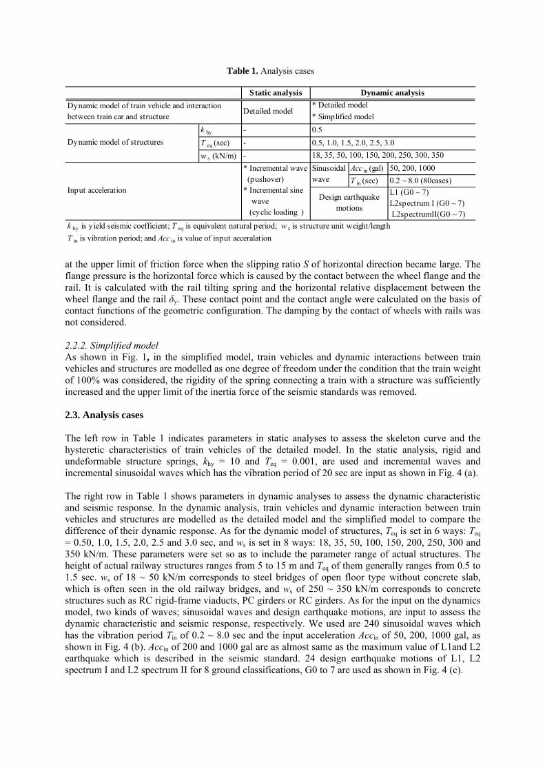
at the upper limit of friction force when the slipping ratio S of horizontal direction became large. The flange pressure is the horizontal force which is caused by the contact between the wheel flange and the rail. It is calculated with the rail tilting spring and the horizontal relative displacement between the wheel flange and the rail δy. These contact point and the contact angle were calculated on the basis of contact functions of the geometric configuration. The damping by the contact of wheels with rails was not considered. 2.2.2. Simplified model As shown in Fig. 1, in the simplified model, train vehicles and dynamic interactions between train vehicles and structures are modelled as one degree of freedom under the condition that the train weight of 100% was considered, the rigidity of the spring connecting a train with a structure was sufficiently increased and the upper limit of the inertia force of the seismic standards was removed. 2.3. Analysis cases The left row in Table 1 indicates parameters in static analyses to assess the skeleton curve and the hysteretic characteristics of train vehicles of the detailed model. In the static analysis, rigid and undeformable structure springs, khy = 10 and Teq = 0.001, are used and incremental waves and incremental sinusoidal waves which has the vibration period of 20 sec are input as shown in Fig. 4 (a). The right row in Table 1 shows parameters in dynamic analyses to assess the dynamic characteristic and seismic response. In the dynamic analysis, train vehicles and dynamic interaction between train vehicles and structures are modelled as the detailed model and the simplified model to compare the difference of their dynamic response. As for the dynamic model of structures, Teq is set in 6 ways: Teq = 0.50, 1.0, 1.5, 2.0, 2.5 and 3.0 sec, and ws is set in 8 ways: 18, 35, 50, 100, 150, 200, 250, 300 and 350 kN/m. These parameters were set so as to include the parameter range of actual structures. The height of actual railway structures ranges from 5 to 15 m and Teq of them generally ranges from 0.5 to 1.5 sec. ws of 18 ~ 50 kN/m corresponds to steel bridges of open floor type without concrete slab, which is often seen in the old railway bridges, and ws of 250 ~ 350 kN/m corresponds to concrete structures such as RC rigid-frame viaducts, PC girders or RC girders. As for the input on the dynamics model, two kinds of waves; sinusoidal waves and design earthquake motions, are input to assess the dynamic characteristic and seismic response, respectively. We used are 240 sinusoidal waves which has the vibration period Tin of 0.2 ~ 8.0 sec and the input acceleration Accin of 50, 200, 1000 gal, as shown in Fig. 4 (b). Accin of 200 and 1000 gal are as almost same as the maximum value of L1and L2 earthquake which is described in the seismic standard. 24 design earthquake motions of L1, L2 spectrum I and L2 spectrum II for 8 ground classifications, G0 to 7 are used as shown in Fig. 4 (c).
Table 1. Analysis cases
Static analysis
k hy -
T eq (sec) -
w s (kN/m) -
Acc in (gal) 50, 200, 1000
T in (sec) 0.2 ~ 8.0 (80cases)
k hy is yield seismic coefficient; T eq is equivalent natural period; w s is structure unit weight/length
T in is vibration period; and Acc in is value of input acceralation
Dynamic analysis
Detailed model* Detailed model
* Simplified model
Dynamic model of structures
Dynamic model of train vehicle and interactionbetween train car and structure
0.5
0.5, 1.0, 1.5, 2.0, 2.5, 3.0
18, 35, 50, 100, 150, 200, 250, 300, 350
Sinusoidalwave
Input acceleration
* Incremental wave (pushover)* Incremental sine wave (cyclic loading )
Design earthquakemotions
L1 (G0 ~ 7)L2spectrum I (G0 ~ 7) L2spectrumII(G0 ~ 7)
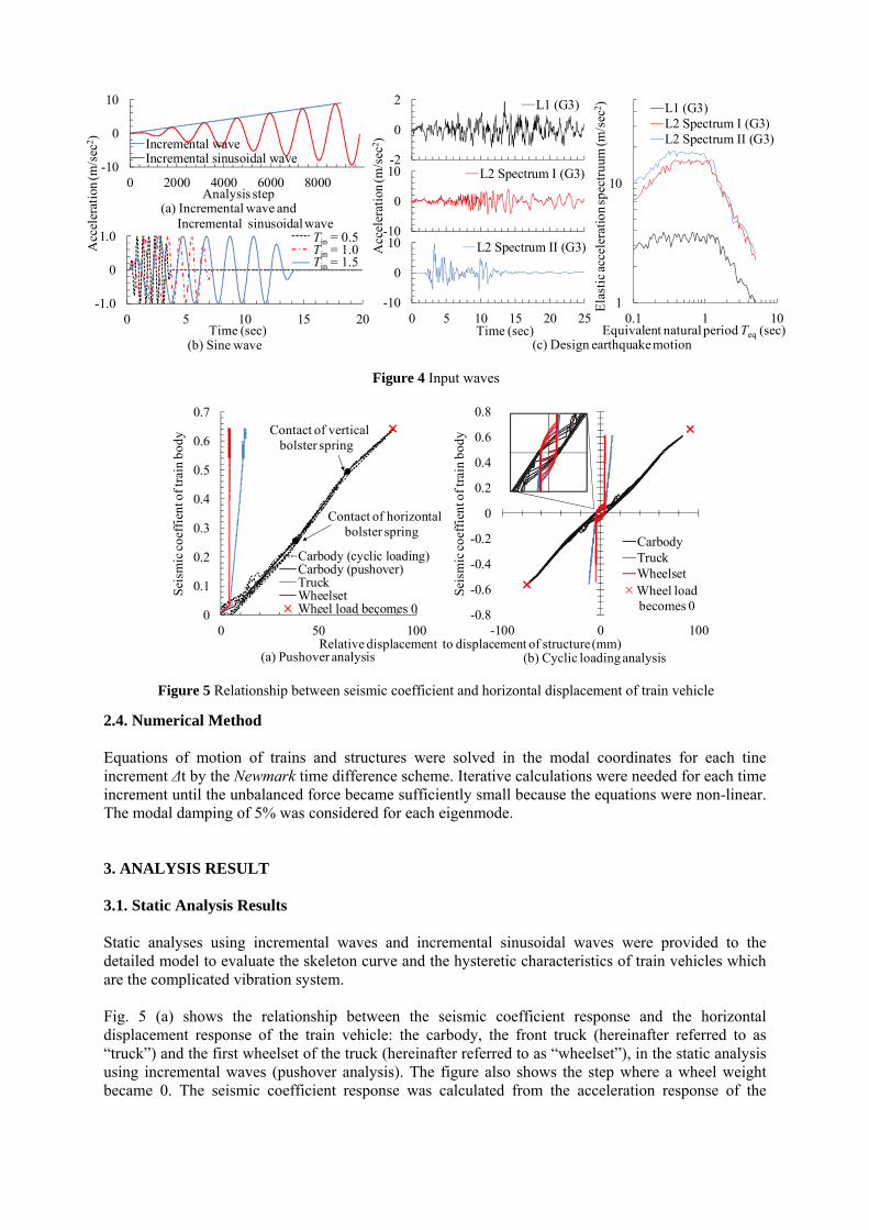
2.4. Numerical Method Equations of motion of trains and structures were solved in the modal coordinates for each tine increment Δt by the Newmark time difference scheme. Iterative calculations were needed for each time increment until the unbalanced force became sufficiently small because the equations were non-linear. The modal damping of 5% was considered for each eigenmode. 3. ANALYSIS RESULT 3.1. Static Analysis Results Static analyses using incremental waves and incremental sinusoidal waves were provided to the detailed model to evaluate the skeleton curve and the hysteretic characteristics of train vehicles which are the complicated vibration system. Fig. 5 (a) shows the relationship between the seismic coefficient response and the horizontal displacement response of the train vehicle: the carbody, the front truck (hereinafter referred to as “truck”) and the first wheelset of the truck (hereinafter referred to as “wheelset”), in the static analysis using incremental waves (pushover analysis). The figure also shows the step where a wheel weight became 0. The seismic coefficient response was calculated from the acceleration response of the
-10
0
10
0 2000 4000 6000 8000
Incremental waveIncremental sinusoidal wave
Acc
eler
atio
n (m
/sec
2 )
Analysis step(a) Incremental wave and
Incremental sinusoidal wave
-1.0
0
1.0
0 5 10 15 20
Tin = 0.5 (s)Tin = 1.0 (s)Tin = 2.0 (s)
(b) Sine wave
-2
0
2
0 5 10 15 20 25
L1 (G3)
-10
0
10
0 5 10 15 20 25
L2 Spectrum I (G3)
-10
0
10
0 5 10 15 20 25
L2 Spectrum II (G3)
Time (sec)(c) Design earthquake motion
Time (sec)
Acc
eler
atio
n (m
/sec
2 )
Equivalent natural period Teq (sec)
Ela
stic
acc
eler
atio
n sp
ectr
uum
(m/s
ec2 )
1
10
0.1 1 10
L1 (G3)L2 Spectrum I (G3)L2 Spectrum II (G3)
Tin = 0.5Tin = 1.0Tin = 1.5
Figure 4 Input waves
-0.8
-0.6
-0.4
-0.2
0
0.2
0.4
0.6
0.8
-100 0 100
CarbodyTruckWheelset
0
0.1
0.2
0.3
0.4
0.5
0.6
0.7
0 50 100
Carbody (cyclic loading)Carbody (pushover)TruckWheelsetWheel load becomes 0
Relative displacement to displacement of structure (mm)
Sei
smic
coe
ffie
nt o
f tra
in b
ody
Sei
smic
coe
ffie
nt o
f tra
in b
ody
-0 .1
0
0 .1
-2 0 0 2 0
(a) Pushover analysis (b) Cyclic loading analysis
Contact of horizontal bolster spring
Contact of vertical bolster spring
Wheel load becomes 0
Figure 5 Relationship between seismic coefficient and horizontal displacement of train vehicle
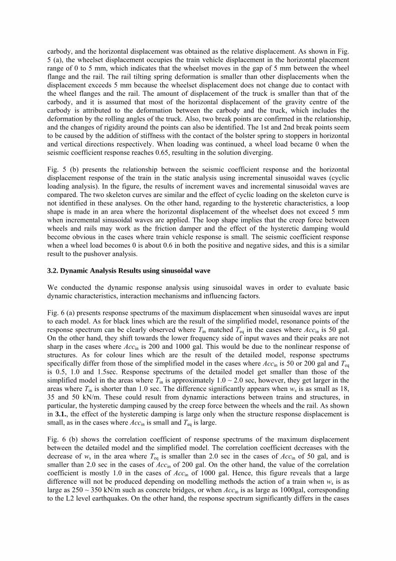
carbody, and the horizontal displacement was obtained as the relative displacement. As shown in Fig. 5 (a), the wheelset displacement occupies the train vehicle displacement in the horizontal placement range of 0 to 5 mm, which indicates that the wheelset moves in the gap of 5 mm between the wheel flange and the rail. The rail tilting spring deformation is smaller than other displacements when the displacement exceeds 5 mm because the wheelset displacement does not change due to contact with the wheel flanges and the rail. The amount of displacement of the truck is smaller than that of the carbody, and it is assumed that most of the horizontal displacement of the gravity centre of the carbody is attributed to the deformation between the carbody and the truck, which includes the deformation by the rolling angles of the truck. Also, two break points are confirmed in the relationship, and the changes of rigidity around the points can also be identified. The 1st and 2nd break points seem to be caused by the addition of stiffness with the contact of the bolster spring to stoppers in horizontal and vertical directions respectively. When loading was continued, a wheel load became 0 when the seismic coefficient response reaches 0.65, resulting in the solution diverging. Fig. 5 (b) presents the relationship between the seismic coefficient response and the horizontal displacement response of the train in the static analysis using incremental sinusoidal waves (cyclic loading analysis). In the figure, the results of increment waves and incremental sinusoidal waves are compared. The two skeleton curves are similar and the effect of cyclic loading on the skeleton curve is not identified in these analyses. On the other hand, regarding to the hysteretic characteristics, a loop shape is made in an area where the horizontal displacement of the wheelset does not exceed 5 mm when incremental sinusoidal waves are applied. The loop shape implies that the creep force between wheels and rails may work as the friction damper and the effect of the hysteretic damping would become obvious in the cases where train vehicle response is small. The seismic coefficient response when a wheel load becomes 0 is about 0.6 in both the positive and negative sides, and this is a similar result to the pushover analysis. 3.2. Dynamic Analysis Results using sinusoidal wave We conducted the dynamic response analysis using sinusoidal waves in order to evaluate basic dynamic characteristics, interaction mechanisms and influencing factors. Fig. 6 (a) presents response spectrums of the maximum displacement when sinusoidal waves are input to each model. As for black lines which are the result of the simplified model, resonance points of the response spectrum can be clearly observed where Tin matched Teq in the cases where Accin is 50 gal. On the other hand, they shift towards the lower frequency side of input waves and their peaks are not sharp in the cases where Accin is 200 and 1000 gal. This would be due to the nonlinear response of structures. As for colour lines which are the result of the detailed model, response spectrums specifically differ from those of the simplified model in the cases where Accin is 50 or 200 gal and Teq is 0.5, 1.0 and 1.5sec. Response spectrums of the detailed model get smaller than those of the simplified model in the areas where Tin is approximately 1.0 ~ 2.0 sec, however, they get larger in the areas where Tin is shorter than 1.0 sec. The difference significantly appears when ws is as small as 18, 35 and 50 kN/m. These could result from dynamic interactions between trains and structures, in particular, the hysteretic damping caused by the creep force between the wheels and the rail. As shown in 3.1., the effect of the hysteretic damping is large only when the structure response displacement is small, as in the cases where Accin is small and Teq is large. Fig. 6 (b) shows the correlation coefficient of response spectrums of the maximum displacement between the detailed model and the simplified model. The correlation coefficient decreases with the decrease of ws in the area where Teq is smaller than 2.0 sec in the cases of Accin of 50 gal, and is smaller than 2.0 sec in the cases of Accin of 200 gal. On the other hand, the value of the correlation coefficient is mostly 1.0 in the cases of Accin of 1000 gal. Hence, this figure reveals that a large difference will not be produced depending on modelling methods the action of a train when ws is as large as 250 ~ 350 kN/m such as concrete bridges, or when Accin is as large as 1000gal, corresponding to the L2 level earthquakes. On the other hand, the response spectrum significantly differs in the cases
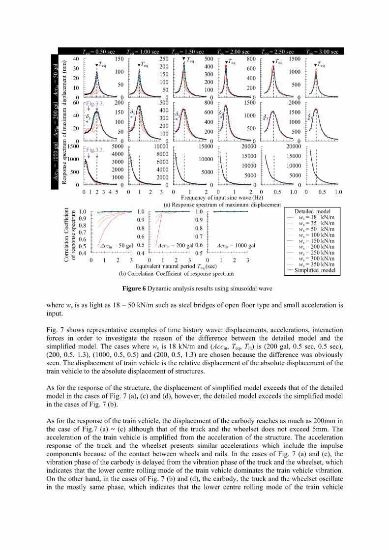
where ws is as light as 18 ~ 50 kN/m such as steel bridges of open floor type and small acceleration is input. Fig. 7 shows representative examples of time history wave: displacements, accelerations, interaction forces in order to investigate the reason of the difference between the detailed model and the simplified model. The cases where ws is 18 kN/m and (Accin, Teq, Tin) is (200 gal, 0.5 sec, 0.5 sec), (200, 0.5, 1.3), (1000, 0.5, 0.5) and (200, 0.5, 1.3) are chosen because the difference was obviously seen. The displacement of train vehicle is the relative displacement of the absolute displacement of the train vehicle to the absolute displacement of structures. As for the response of the structure, the displacement of simplified model exceeds that of the detailed model in the cases of Fig. 7 (a), (c) and (d), however, the detailed model exceeds the simplified model in the cases of Fig. 7 (b). As for the response of the train vehicle, the displacement of the carbody reaches as much as 200mm in the case of Fig.7 (a) ~ (c) although that of the truck and the wheelset does not exceed 5mm. The acceleration of the train vehicle is amplified from the acceleration of the structure. The acceleration response of the truck and the wheelset presents similar accelerations which include the impulse components because of the contact between wheels and rails. In the cases of Fig. 7 (a) and (c), the vibration phase of the carbody is delayed from the vibration phase of the truck and the wheelset, which indicates that the lower centre rolling mode of the train vehicle dominates the train vehicle vibration. On the other hand, in the cases of Fig. 7 (b) and (d), the carbody, the truck and the wheelset oscillate in the mostly same phase, which indicates that the lower centre rolling mode of the train vehicle
0
10
20
30
40
0 1 2 3 4 5
0
20
40
60
0 1 2 3 4 5
0
500
1000
1500
0 1 2 3 4 5
0
50
100
150
0 1 2 3
0
50
100
150
200
0 1 2 3
010002000300040005000
0 1 2 30
2000400060008000
10000
0 1 2
050
100150200250
0 1 2
0100200300400500
0 1 2
0100200300400500
0 1 2
0
200
400
600
800
0 1 2
0
5000
10000
15000
0 1 20
5000
10000
15000
20000
0 0.5 1.0
0
200
400
600
800
0 0.5 1.0
0
500
1000
1500
0 0.5 1.0
0
500
1000
1500
0 0.5 1.0
0
500
1000
1500
2000
0 0.5 1.0
0
5000
10000
15000
20000
0 0.5 1.0Frequency of input sine wave (Hz)
0.40.50.60.70.80.91.0
0 1 2 30.4
0.5
0.6
0.8
0.9
1.0
0 1 2 30.5
0.6
0.7
0.8
0.9
1.0
0 1 2 3
Res
pons
e sp
ectr
um o
f m
axim
um d
ispl
acem
ent
(mm
)C
orre
latio
n C
oeff
icie
nt
of r
espo
nse
spec
trum
Equivalent natural period Teq (sec)
(a) Response spectrum of maximum displacement
(b) Correlation Coefficient of response spectrum
Teq = 0.50 sec Teq = 1.00 sec Teq = 1.50 sec Teq = 2.00 sec Teq = 2.50 sec Teq = 3.00 secA
ccin
= 1
000
gal
Acc
in=
200
gal
A
ccin
= 5
0 ga
l
Detailed modelws = 18 kN/mws = 35 kN/mws = 50 kN/mws = 100 kN/mws = 150 kN/mws = 200 kN/mws = 250 kN/mws = 300 kN/mws = 350 kN/m
Simplified model
Teq TeqTeq Teq Teq Teq
Accin = 1000 galAccin = 200 galAccin = 50 gal
δyδyδyδy
δyδy
Fig.3.3.
Fig.3.3.
Figure 6 Dynamic analysis results using sinusoidal wave
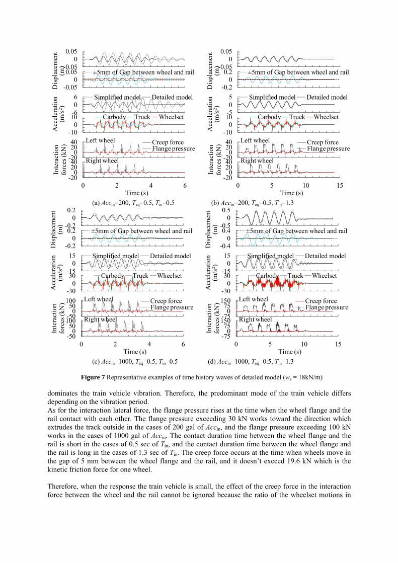
dominates the train vehicle vibration. Therefore, the predominant mode of the train vehicle differs depending on the vibration period. As for the interaction lateral force, the flange pressure rises at the time when the wheel flange and the rail contact with each other. The flange pressure exceeding 30 kN works toward the direction which extrudes the track outside in the cases of 200 gal of Accin, and the flange pressure exceeding 100 kN works in the cases of 1000 gal of Accin. The contact duration time between the wheel flange and the rail is short in the cases of 0.5 sec of Tin, and the contact duration time between the wheel flange and the rail is long in the cases of 1.3 sec of Tin. The creep force occurs at the time when wheels move in the gap of 5 mm between the wheel flange and the rail, and it doesn’t exceed 19.6 kN which is the kinetic friction force for one wheel. Therefore, when the response the train vehicle is small, the effect of the creep force in the interaction force between the wheel and the rail cannot be ignored because the ratio of the wheelset motions in
-0.050
0.05
0 2 4 6
-0.050
0.05
0 2 4 6
±5mm of Gap between wheel and rail
-606
0 2 4 6
Simplified model Detailed model
-100
10
0 2 4 6
Carbody Truck Wheelset
-200
2040
0 2 4 6
-200
2040
0 2 4 6
Dis
plac
emen
t(m
)A
ccel
erat
ion
(m/s
2 )
Creep forceFlange pressure
Inte
ract
ion
forc
es (k
N)
Left wheel
Right wheel
Time (s)
-0.050
0.05
0 5 10 15
-0.20
0.2
0 5 10 15
±5mm of Gap between wheel and rail
-505
0 5 10 15
Simplified model Detailed model
-100
10
0 5 10 15
Carbody Truck Wheelset
-200
2040
0 5 10 15
-200
2040
0 5 10 15
Dis
plac
emen
t(m
)A
ccel
erat
ion
(m/s
2 )
Creep forceFlange pressure
Inte
ract
ion
forc
es (k
N)
Left wheel
Right wheel
Time (s)
(a) Accin=200, Teq=0.5, Tin=0.5 (b) Accin=200, Teq=0.5, Tin=1.3
-0.20
0.2
0 2 4 6
-0.20
0.2
0 2 4 6
±5mm of Gap between wheel and rail
-150
15
0 2 4 6
Simplified model Detailed model
-300
30
0 2 4 6
Carbody Truck Wheelset
-500
50100
0 2 4 6
-500
50100
0 2 4 6
Dis
plac
emen
t(m
)A
ccel
erat
ion
(m/s
2 )
Creep forceFlange pressure
Inte
ract
ion
forc
es (k
N)
Left wheel
Right wheel
Time (s)
-0.50
0.5
0 5 10 15
-0.40
0.4
0 5 10 15
±5mm of Gap between wheel and rail
-150
15
0 5 10 15
Simplified model Detailed model
-300
30
0 5 10 15
Carbody Truck Wheelset
-750
75150
0 5 10 15
-750
75150
0 5 10 15
Dis
plac
emen
t(m
)A
ccel
erat
ion
(m/s
2 )
Creep forceFlange pressure
Inte
ract
ion
forc
es (k
N)
Left wheel
Right wheel
Time (s) (c) Accin=1000, Teq=0.5, Tin=0.5 (d) Accin=1000, Teq=0.5, Tin=1.3
Figure 7 Representative examples of time history waves of detailed model (ws = 18kN/m)
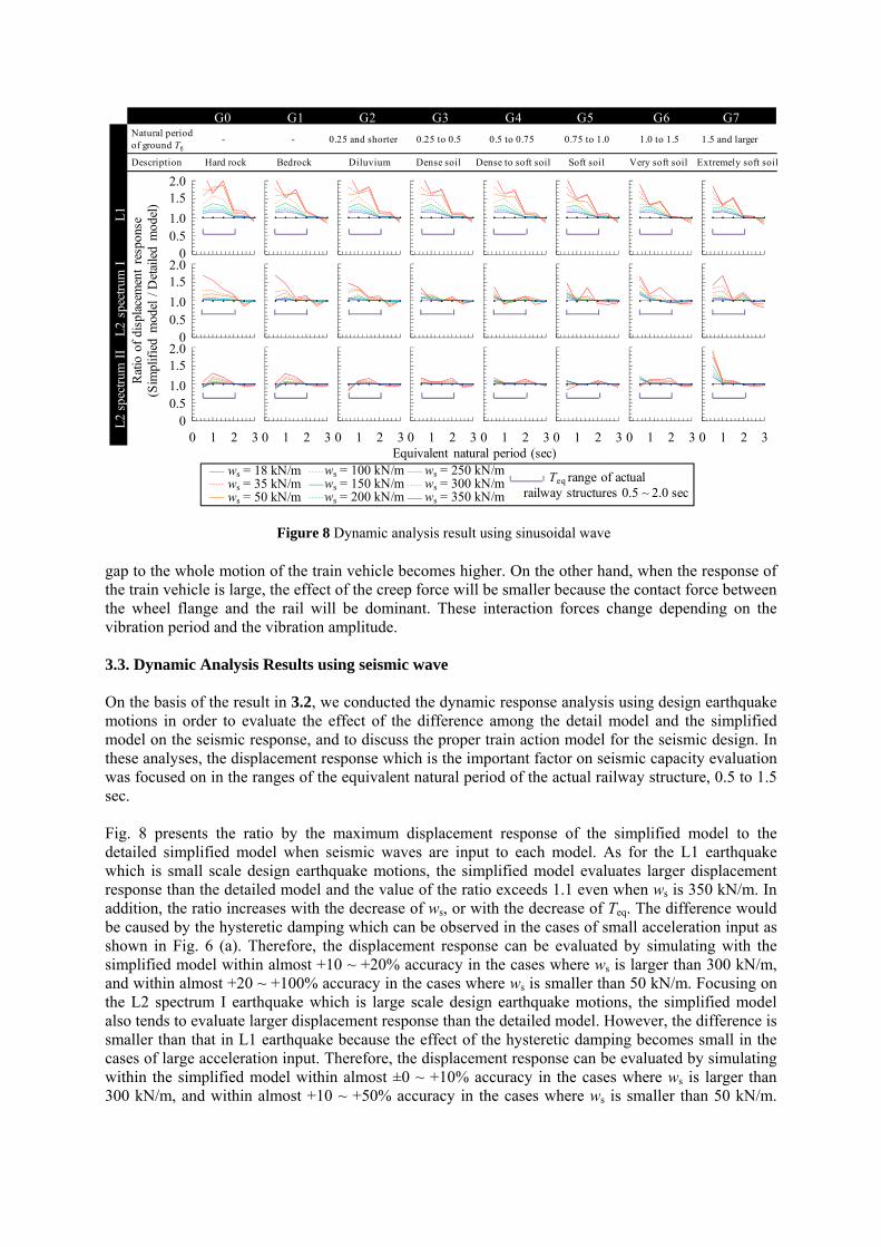
gap to the whole motion of the train vehicle becomes higher. On the other hand, when the response of the train vehicle is large, the effect of the creep force will be smaller because the contact force between the wheel flange and the rail will be dominant. These interaction forces change depending on the vibration period and the vibration amplitude. 3.3. Dynamic Analysis Results using seismic wave On the basis of the result in 3.2, we conducted the dynamic response analysis using design earthquake motions in order to evaluate the effect of the difference among the detail model and the simplified model on the seismic response, and to discuss the proper train action model for the seismic design. In these analyses, the displacement response which is the important factor on seismic capacity evaluation was focused on in the ranges of the equivalent natural period of the actual railway structure, 0.5 to 1.5 sec. Fig. 8 presents the ratio by the maximum displacement response of the simplified model to the detailed simplified model when seismic waves are input to each model. As for the L1 earthquake which is small scale design earthquake motions, the simplified model evaluates larger displacement response than the detailed model and the value of the ratio exceeds 1.1 even when ws is 350 kN/m. In addition, the ratio increases with the decrease of ws, or with the decrease of Teq. The difference would be caused by the hysteretic damping which can be observed in the cases of small acceleration input as shown in Fig. 6 (a). Therefore, the displacement response can be evaluated by simulating with the simplified model within almost +10 ~ +20% accuracy in the cases where ws is larger than 300 kN/m, and within almost +20 ~ +100% accuracy in the cases where ws is smaller than 50 kN/m. Focusing on the L2 spectrum I earthquake which is large scale design earthquake motions, the simplified model also tends to evaluate larger displacement response than the detailed model. However, the difference is smaller than that in L1 earthquake because the effect of the hysteretic damping becomes small in the cases of large acceleration input. Therefore, the displacement response can be evaluated by simulating within the simplified model within almost ±0 ~ +10% accuracy in the cases where ws is larger than 300 kN/m, and within almost +10 ~ +50% accuracy in the cases where ws is smaller than 50 kN/m.
Teq range of actual railway structures 0.5 ~ 2.0 sec
0
0.5
1.0
1.5
2.0
0 1 2 3
0
0.5
1.0
1.5
2.0
0 1 2 3
0
0.5
1.0
1.5
2.0
0 1 2 3
0
0.5
1.0
1.5
2.0
0 1 2 3
0
0.5
1.0
1.5
2.0
0 1 2 3
0
0.5
1.0
1.5
2.0
0 1 2 3
0
0.5
1.0
1.5
2.0
0 1 2 3
0
0.5
1.0
1.5
2.0
0 1 2 3
0
0.5
1.0
1.5
2.0
0 1 2 3
0
0.5
1.0
1.5
2.0
0 1 2 3
0
0.5
1.0
1.5
2.0
0 1 2 3
0
0.5
1.0
1.5
2.0
0 1 2 3
0
0.5
1.0
1.5
2.0
0 1 2 3
0
0.5
1.0
1.5
2.0
0 1 2 3
0
0.5
1.0
1.5
2.0
0 1 2 3
0
0.5
1.0
1.5
2.0
0 1 2 3
0
0.5
1.0
1.5
2.0
0 1 2 3
0
0.5
1.0
1.5
2.0
0 1 2 3
0
0.5
1.0
1.5
2.0
0 1 2 3
0
0.5
1.0
1.5
2.0
0 1 2 3
0
0.5
1.0
1.5
2.0
0 1 2 3
0
0.5
1.0
1.5
2.0
0 1 2 3
0
0.5
1.0
1.5
2.0
0 1 2 3
0
0.5
1.0
1.5
2.0
0 1 2 3Equivalent natural period (sec)
Rat
io o
f di
spla
cem
ent
resp
onse
(S
impl
ifie
d m
odel
/ D
etai
led
mod
el)
G0 G1 G2 G3 G4 G5 G6 G7L
2 sp
ectr
um I
I L
2 sp
ectr
um I
L
1
ws = 18 kN/mws = 35 kN/mws = 50 kN/m
ws = 100 kN/mws = 150 kN/mws = 200 kN/m
ws = 250 kN/mws = 300 kN/mws = 350 kN/m
1.5
1.00.5
0
2.0
1.5
1.00.5
0
2.0
1.5
1.00.5
0
2.0
- - 0.25 and shorter 0.25 to 0.5 0.5 to 0.75 0.75 to 1.0 1.0 to 1.5 1.5 and largerNatural period of ground Tg
Description Hard rock Bedrock Diluvium Dense soil Dense to soft soil Soft soil Very soft soil Extremely soft soil
Figure 8 Dynamic analysis result using sinusoidal wave
From the results of the L2 spectrum II earthquake, the simplified model evaluates larger displacement response than the detailed model in almost cases although it underestimates the displacement response in some cases; especially in the cases where Teq is 0.5 sec. However, the difference is the smallest in all design earthquake motions, which seems to because the effect of the hysteretic damping is small and the number of cyclic loading caused by L2 spectrum II earthquake is low. Hence, the displacement response can be evaluated by simulating within the simplified model within almost ±5% accuracy in the cases where ws is larger than 300 kN/m, and within almost -20 ~ +30% accuracy in the cases where ws is smaller than 50 kN/m. Consequently, the simplified model can evaluate the displacement response of heavy structures such as concreted bridges during earthquake with +10 ~ +20% accuracy as for L1 earthquake, and with adequate accuracy as for L2 earthquake. On the other hand, it can evaluate the displacement response of light structures such as steel bridges of open floor type with +20 ~ +100% accuracy as for L1 earthquake, and with -20 ~ +50% accuracy as for L2 earthquake. As the simplified model doesn’t have an adequate accuracy, it is preferable to evaluate the displacement response during earthquake with considering the effect of dynamic interactions between train vehicles and structures using an interaction analysis program such as DIASTARS. 4. CONCLUSION This paper aims to quantify dynamic interactions between train vehicles and railway structures during earthquakes, and to develop a reasonable train action model. As the result of numerical simulation on the basis of precise train model and contact model between rails and wheel, this paper has obtained the following conclusions. (1) Dynamic interactions between train vehicles and railway structures can be mainly controlled by
the creep force in the case of small response of train vehicles, and by the contact force between wheels flange and rails in the case of large response of train vehicles.
(2) The displacement response of heavy structures, such as RC structures, during earthquake can be evaluated without considering the effect of dynamic interactions with +10 ~ +20% accuracy as for L1 earthquake, and with adequate accuracy as for L2 earthquake.
(3) The displacement response of light structures, such as steel bridges of open floor type, during earthquake should be evaluated with considering the effect of dynamic interactions between train vehicles and structures using an interaction analysis program such as DIASTARS because the accuracy of the simplified model is inadequate, +20 ~ +100% for L1 earthquake, and -20 ~ +50% for L2 earthquake.
REFERENCES Wakui, H., Matsumoto, N., and Tanabe, M. (1994). A Study on Dynamic Interaction Analysis for Railway
Vehicles and Structures - Mechanical model and practical analysis method -. Quarterly Report of RTRI. Vol.35: No.2, 96-104.
Railway Technical Research Institute (1999). Design Standards for Railway Structures and Commentary (Seismic Design), Maruzen Co., Ltd, Tokyo (in Japanese)
Railway Technical Research Institute (2006). Design Standards for Railway Structures and Commentary (Seismic Design) A guideline of Seismic Verification (in Japanese)
Railway Technical Research Institute (2008). Design Standards for Railway Structures and Commentary (Concrete Structure) An Example of Seismic Verification for a RC Railway Rigid-Frame Viaduct (in Japanese)
Miyamoto, T., Matsumoto, N., Sogabe, M., Shimomura, T., Nishiyama, Y. and Matsuo, M. (2007). Full-scale Experiment on Dynamic Behavior of Railway Vehicle against Heavy Track Vibration. Journal of Environment and Engineering. Vol.2: No.2, 419-428.