EED version 4 within building physics and ground heat storage BLOCON EED version 4 Earth Energy Designer Update manual Nov 30, 2016 ... 3 Contents 1

Software within building physics and ground heat storage

BLOCON

www.buildingphysics.com

EED version 4 Earth Energy Designer

Update manual

Nov 30, 2016

Revised March 1, 2017

See Appendix for update news.

http://www.buildingphysics.com/

2

3

Contents

1. INTRODUCTION ............................................................................................................ 5

1.1 WHAT’S NEW IN EED V4 ............................................................................................. 5 1.2 DEMO VERSION ............................................................................................................ 5 1.3 INSTALLATION AND REQUIREMENTS ........................................................................... 5 1.4 ACTIVATION AND DEACTIVATION OF EED .................................................................. 6

2. SOME CHANGES COMPARE TO EED V3 ................................................................ 7

2.1 SIMULATIONS F9 AND F10 ........................................................................................... 7 2.2 QUICKER AND BETTER OPTIMIZATION ....................................................................... 10

3. SIMULATIONS WITH HOURLY VALUES .............................................................. 13

3.1 INTRODUCTION .......................................................................................................... 13 3.2 NOTE ON CALCULATION TIMES .................................................................................. 13 3.3 SPECIFYING DATA FOR HOURLY VALUES ................................................................... 14 3.4 DATE FORMATS .......................................................................................................... 21 3.5 EXAMPLE (HOURLY_EXAMPLE_1.DAT) .................................................................... 22 3.6 OPTIMIZATION FOR HOURLY VALUES ........................................................................ 35 3.7 EXPORTING DATA ...................................................................................................... 36 3.8 EWT AND LWT ......................................................................................................... 38

4. APPROXIMATION FOR IRREGULAR CONFIGURATIONS [UPDATED IN V4.14] 39

4.1 INTRODUCTION .......................................................................................................... 39 4.2 TEST OF APPROXIMATION, EXAMPLE 1 ...................................................................... 43 4.3 TEST OF APPROXIMATION, EXAMPLE 2 ...................................................................... 45

5. CHANGEABLE USER INTERFACE OF EED .......................................................... 48

5.1 INTRODUCTION .......................................................................................................... 48

6. FASTER HOURLY SIMULATIONS [AVAILABLE IN V4.14] ............................... 50

6.1 INTRODUCTION .......................................................................................................... 50 6.2 OPTIONS FOR CALCULATIONS .................................................................................... 51 6.3 BENCHMARKS FOR F9 (“SOLVE MEAN FLUID TEMPERATURES”)............................... 52 6.4 BENCHMARKS FOR F10 (“SOLVE REQUIRED BOREHOLE LENGTH”) .......................... 53

4

5

1. Introduction Blocon is proud to present a new version of EED. Many new important features have been added. Up-

to-date information is given on www.buildingphysics.com.

This update manual covers new features that have been added since version 3. New users should also

read the full manual for version 3 at

http://www.buildingphysics.com/manuals/EED3.pdf

Please see this page for some questions/answers:

http://www.buildingphysics.com/index-filer/Page1139.htm

This manual covers the desktop version of EED v4. There is also an optional web version: “EED on

the web” that runs on a dedicated server with extreme calculation performance. It can be started from

any operating system and/or device with an HTML5-compliant web browser, such as IE10/11,

Chrome, Safari, Firefox, Opera, etc. It supports PC, Mac, iPad, iPhone, Chromebook, Android and

many other popular devices. For more info, see:

http://www.buildingphysics.com/manuals/EEDONTHEWEB.pdf

1.1 What’s new in EED v4

The most important new feature is the following:

Simulations with hourly values for load are possible. See Chapters 2 and 3.

Approximation for irregular configurations. See Chapter 4.

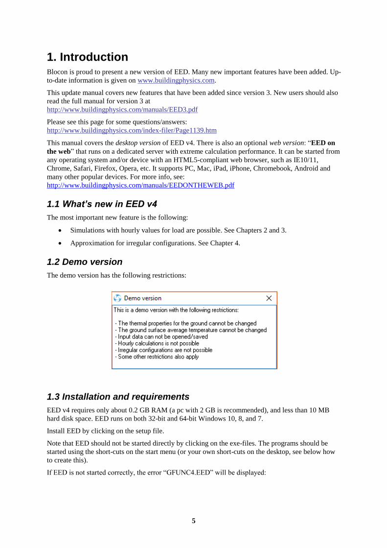
1.2 Demo version

The demo version has the following restrictions:

1.3 Installation and requirements

EED v4 requires only about 0.2 GB RAM (a pc with 2 GB is recommended), and less than 10 MB

hard disk space. EED runs on both 32-bit and 64-bit Windows 10, 8, and 7.

Install EED by clicking on the setup file.

Note that EED should not be started directly by clicking on the exe-files. The programs should be

started using the short-cuts on the start menu (or your own short-cuts on the desktop, see below how

to create this).

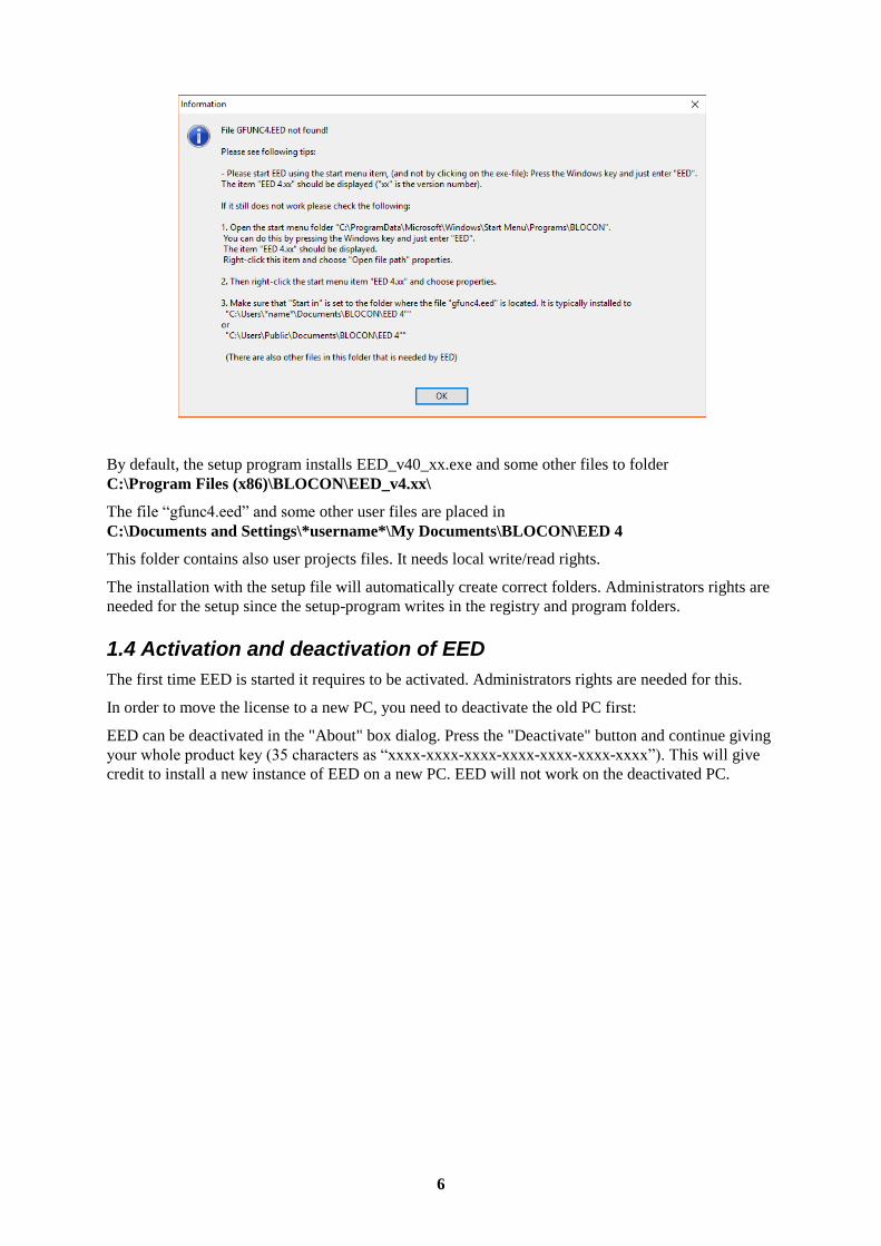
If EED is not started correctly, the error “GFUNC4.EED” will be displayed:

http://www.buildingphysics.com/manuals/EED3.pdf



6

By default, the setup program installs EED_v40_xx.exe and some other files to folder

C:\Program Files (x86)\BLOCON\EED_v4.xx\

The file “gfunc4.eed” and some other user files are placed in

C:\Documents and Settings\*username*\My Documents\BLOCON\EED 4

This folder contains also user projects files. It needs local write/read rights.

The installation with the setup file will automatically create correct folders. Administrators rights are

needed for the setup since the setup-program writes in the registry and program folders.

1.4 Activation and deactivation of EED

The first time EED is started it requires to be activated. Administrators rights are needed for this.

In order to move the license to a new PC, you need to deactivate the old PC first:

EED can be deactivated in the "About" box dialog. Press the "Deactivate" button and continue giving

your whole product key (35 characters as “xxxx-xxxx-xxxx-xxxx-xxxx-xxxx-xxxx”). This will give

credit to install a new instance of EED on a new PC. EED will not work on the deactivated PC.

7

2. Some changes compare to EED v3

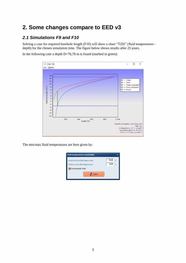
2.1 Simulations F9 and F10

Solving a case for required borehole length (F10) will show a chart “T(D)” (fluid temperatures –

depth) for the chosen simulation time. The figure below shows results after 25 years.

In the following case a depth D=76,78 m is found (marked in green):

The min/max fluid temperatures are here given by:

8

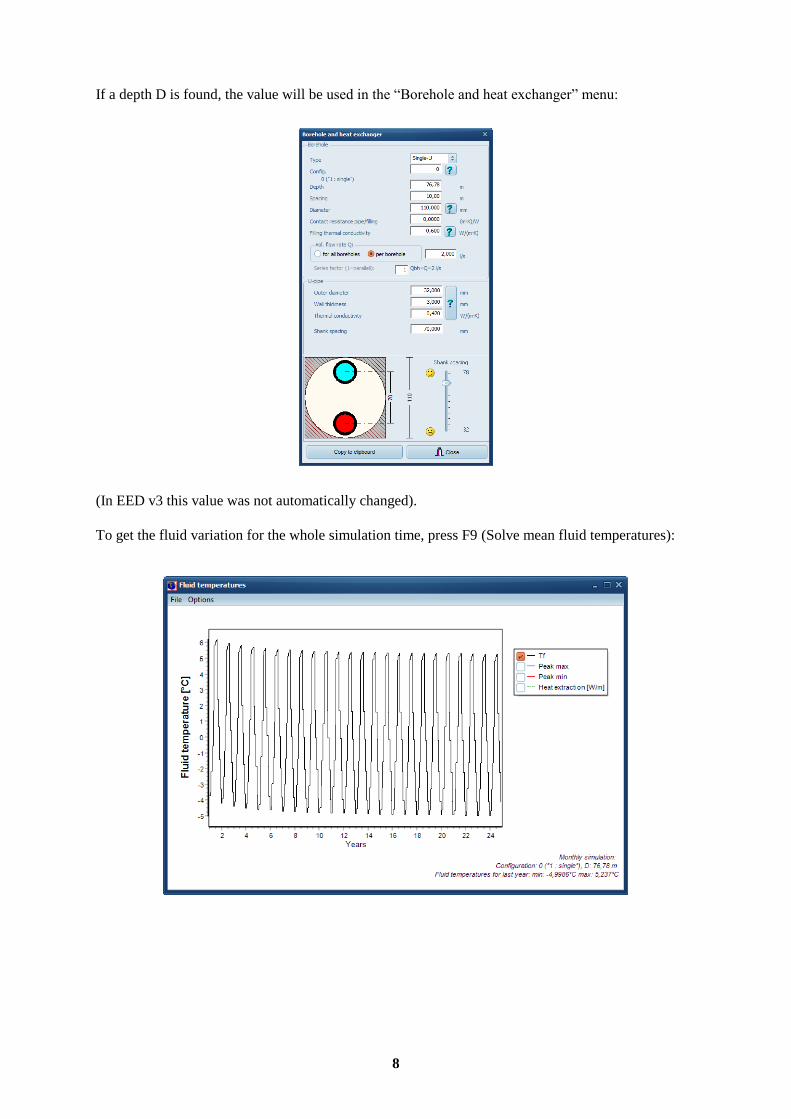
If a depth D is found, the value will be used in the “Borehole and heat exchanger” menu:

(In EED v3 this value was not automatically changed).

To get the fluid variation for the whole simulation time, press F9 (Solve mean fluid temperatures):

9

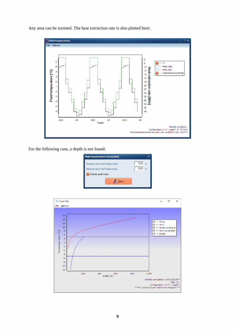
Any area can be zoomed. The heat extraction rate is also plotted here:

For the following case, a depth is not found:

10

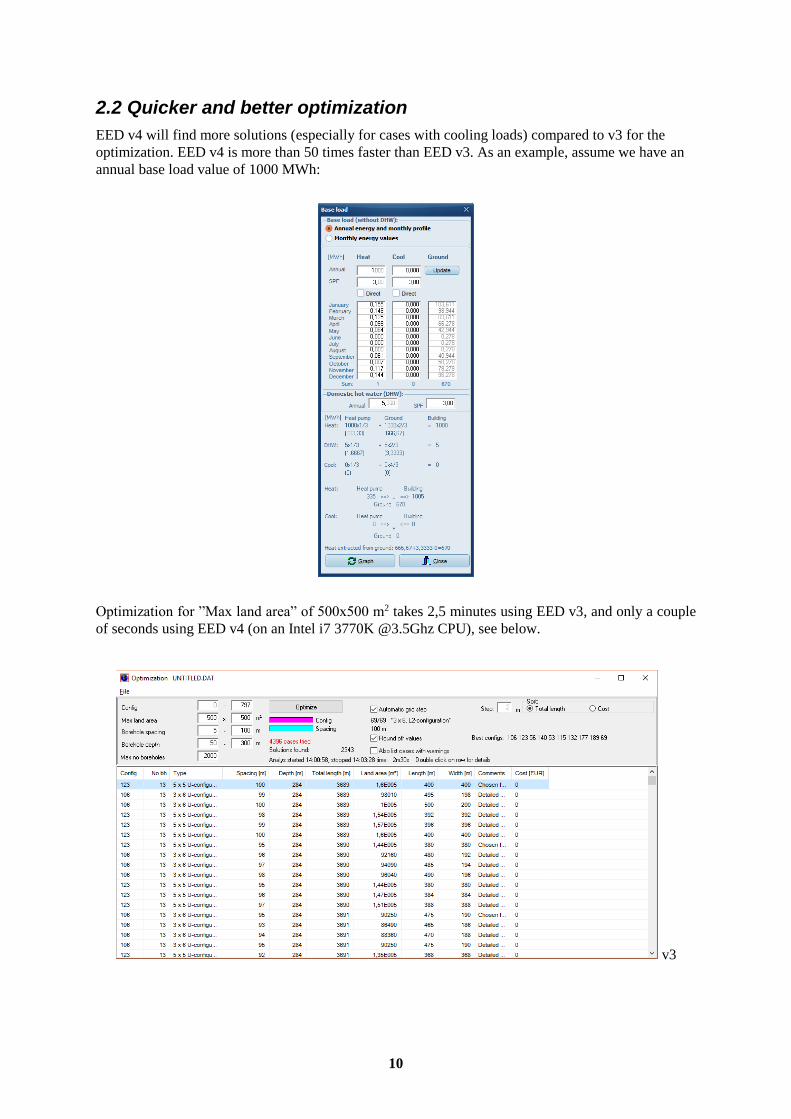
2.2 Quicker and better optimization

EED v4 will find more solutions (especially for cases with cooling loads) compared to v3 for the

optimization. EED v4 is more than 50 times faster than EED v3. As an example, assume we have an

annual base load value of 1000 MWh:

Optimization for ”Max land area” of 500x500 m2 takes 2,5 minutes using EED v3, and only a couple

of seconds using EED v4 (on an Intel i7 3770K @3.5Ghz CPU), see below.

v3

11

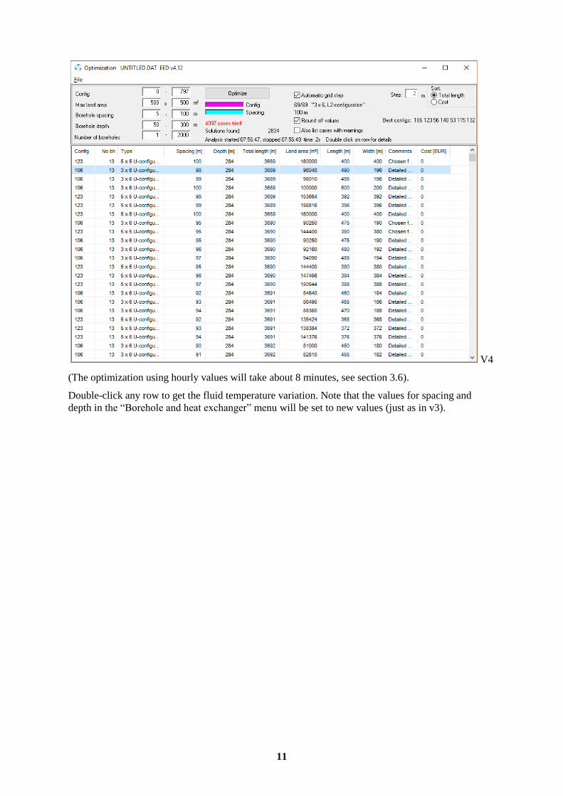
V4

(The optimization using hourly values will take about 8 minutes, see section 3.6).

Double-click any row to get the fluid temperature variation. Note that the values for spacing and

depth in the “Borehole and heat exchanger” menu will be set to new values (just as in v3).

12

13

3. Simulations with hourly values

3.1 Introduction

EED v4 can calculate the response due to any hourly load variation. This means that it handles any

loads for cooling, heating, and DHW (District Heat Water), with a resolution of one hour.

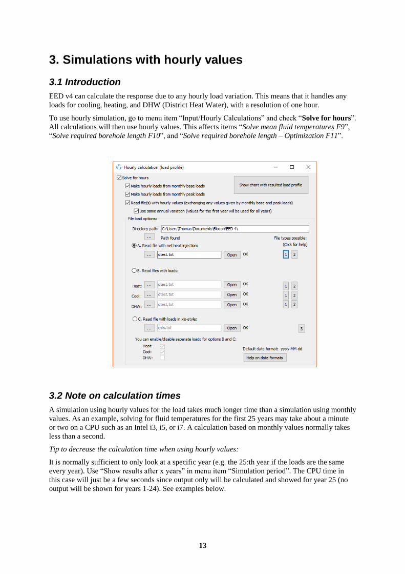
To use hourly simulation, go to menu item “Input/Hourly Calculations” and check “Solve for hours”.

All calculations will then use hourly values. This affects items “Solve mean fluid temperatures F9”,

“Solve required borehole length F10”, and “Solve required borehole length – Optimization F11”.

3.2 Note on calculation times

A simulation using hourly values for the load takes much longer time than a simulation using monthly

values. As an example, solving for fluid temperatures for the first 25 years may take about a minute

or two on a CPU such as an Intel i3, i5, or i7. A calculation based on monthly values normally takes

less than a second.

Tip to decrease the calculation time when using hourly values:

It is normally sufficient to only look at a specific year (e.g. the 25:th year if the loads are the same

every year). Use “Show results after x years” in menu item “Simulation period”. The CPU time in

this case will just be a few seconds since output only will be calculated and showed for year 25 (no

output will be shown for years 1-24). See examples below.

14

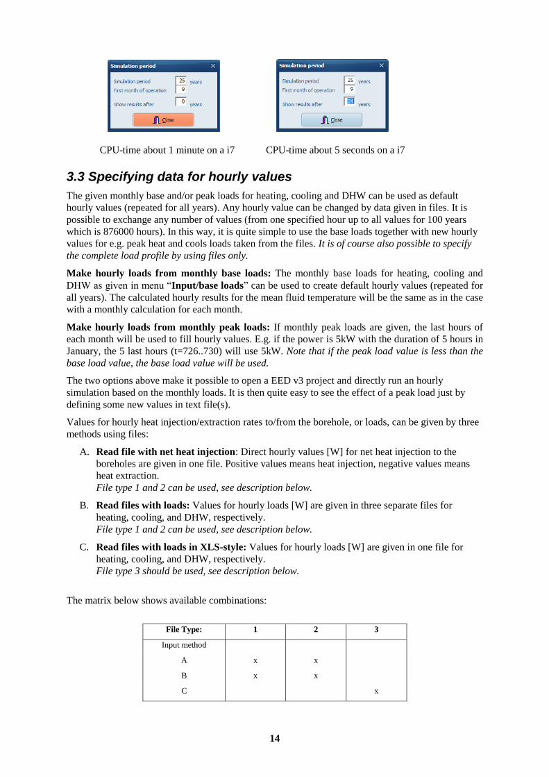
CPU-time about 1 minute on a i7 CPU-time about 5 seconds on a i7

3.3 Specifying data for hourly values

The given monthly base and/or peak loads for heating, cooling and DHW can be used as default

hourly values (repeated for all years). Any hourly value can be changed by data given in files. It is

possible to exchange any number of values (from one specified hour up to all values for 100 years

which is 876000 hours). In this way, it is quite simple to use the base loads together with new hourly

values for e.g. peak heat and cools loads taken from the files. It is of course also possible to specify

the complete load profile by using files only.

Make hourly loads from monthly base loads: The monthly base loads for heating, cooling and

DHW as given in menu “Input/base loads” can be used to create default hourly values (repeated for

all years). The calculated hourly results for the mean fluid temperature will be the same as in the case

with a monthly calculation for each month.

Make hourly loads from monthly peak loads: If monthly peak loads are given, the last hours of

each month will be used to fill hourly values. E.g. if the power is 5kW with the duration of 5 hours in

January, the 5 last hours (t=726..730) will use 5kW. Note that if the peak load value is less than the

base load value, the base load value will be used.

The two options above make it possible to open a EED v3 project and directly run an hourly

simulation based on the monthly loads. It is then quite easy to see the effect of a peak load just by

defining some new values in text file(s).

Values for hourly heat injection/extraction rates to/from the borehole, or loads, can be given by three

methods using files:

A. Read file with net heat injection: Direct hourly values [W] for net heat injection to the

boreholes are given in one file. Positive values means heat injection, negative values means

heat extraction.

File type 1 and 2 can be used, see description below.

B. Read files with loads: Values for hourly loads [W] are given in three separate files for

heating, cooling, and DHW, respectively.

File type 1 and 2 can be used, see description below.

C. Read files with loads in XLS-style: Values for hourly loads [W] are given in one file for

heating, cooling, and DHW, respectively.

File type 3 should be used, see description below.

The matrix below shows available combinations:

File Type: 1 2 3

Input method

A x x

B x x

C x

15

The heat injected to the boreholes for each hour for method B and C is calculated as

qinjected=qheat*(spfh-1.0)/spfh + qcool*(spfc+1.0)/ spfc + qdhw*(spfdhw-1.0)/spfdhw

Note that all heat flows are here defined as positive from the ground to the borehole which means that

the values in the files for heating and DHW loads should be negative (heat is extracted from

boreholes), while the cooling load values should be positive (heat is injected).

Also note that the SPF values for heat, cooling, and DHW are the same as the ones given in menu

“Input/base loads”.

It is possible to enable/disable to use any of the loads by checking Use.

The heat injection rates, and loads, are given for the whole system (i.e. for all boreholes) in [W]. EED

will divide the values with the number of boreholes and the depth for the current configuration and

present results in W/m (i.e. per meter borehole).

If Use same annual variation (using data for year 1) is checked, the load profile for the first year

will be used for all years (even though the file(s) have values for t>1 year).

Any text file can be opened in the Notepad editor by pressing Open (if it already is open press Alt-

Tab to toggle between EED and Notepad). The files will be re-read whenever a simulation is started

(F9, F10, or F11). Remember to save the file before starting any analysis.

Tip: Since there are many ways to give input for loads it is a good idea to check that resulting data

are correct. The chart “Show chart with resulted load profile” will show the final heat

injected/extracted to/from boreholes that is used for the simulation.

16

Format for files

There are three ways how to specify data in files, see type 1, 2, and 3 below. The first row in a file

should contain the type number followed by an optional factor that is multiplied with the values read.

Values are assumed to be in [W]. If values are given in kW, the factor should be 1000. The factor

may also be negative, e.g. “-1” will change values taken from a heating load file (with negative values

since heat is extracted) to positive values which means heat injection (cooling load), and vice versa. It

is also quite easy to use this factor in order to see the effect if loads are raised by e.g. 10% (factor

1.1), lowered by 20% (factor 0.8), or doubled (factor 2). Comments can be added after the data, or on

a separate line that starts with “%”. Blocks can be commented out by “{“ and “}”.

Default load values are given in SI units as [W], but can also be given in Imperial units as [BTU/h].

The decimal mark for load values can be both a dot (“.”) or a comma (“,”). EED will automatically

recognize e.g. “45.2” and “45,2” as the same value.

File type 1. Hourly values (q0, q1, q2…) given as a list. Maximum number is 876000 (100 years).

Normally 8760 values are given in order to specify data for a year.

row 1: [type] [factor] (optional) example: “1 1000”

following rows:

(optional) [dateformat] [string] example: "dateformat ymd"

(optional) [dateseparator] [string] example: "dateseparator -"

(optional) [BTU] Input given in BTU/h instead of in W (1W=3.41214 btu/hour)

(optional) [date] example: "2006-03-21" or "2006-03-21 10:00"

[value] example: “45.2”

The parameters [dateformat] and [dateseparator] are described in a separate section below.

The optional [date] row specifies when hourly data is started for a specific year. The date can be

given as:

“2006-03-21 00:00:00”, or "2006-03-21 00:00", or just “2006-03-21”, will give start index

t=1896h (it has passed 79 days, i.e. 79*24=1896h, to this date and time for year 2006) which

means that the first value read (on third row) will have index q1896, the second value q1897,

and so on. Since data is not given for q0..q1895, values from base loads will be used if that

option is checked, otherwise zeros.

“2006-03-21 05:00:00”, or just “2006-03-21 5” will give start index t=1901h which means

that the first value read will have index q1901, the second value q1902, and so on.

If no row is given, the start time is assumed to be t=0, and the first value read will have index 0

(“q0”). The start time can be different in e.g. the load files for heating, cooling, and DHW.

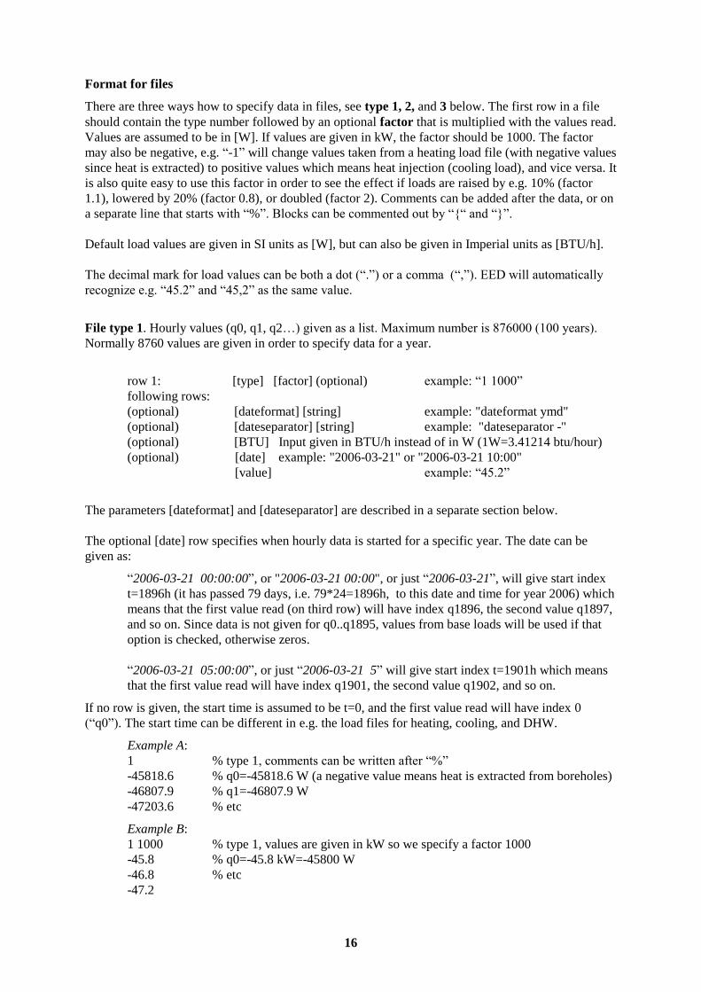
Example A:

1 % type 1, comments can be written after “%”

-45818.6 % q0=-45818.6 W (a negative value means heat is extracted from boreholes)

-46807.9 % q1=-46807.9 W

-47203.6 % etc

Example B:

1 1000 % type 1, values are given in kW so we specify a factor 1000

-45.8 % q0=-45.8 kW=-45800 W

-46.8 % etc

-47.2

17

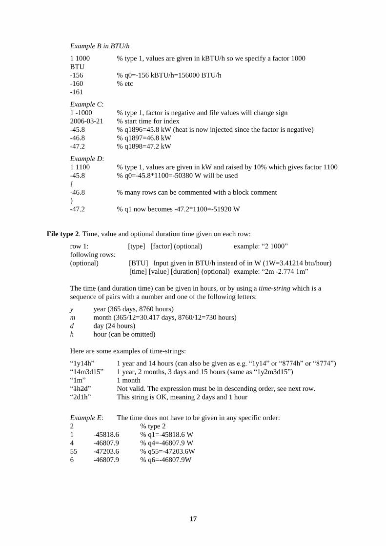
Example B in BTU/h

1 1000 % type 1, values are given in kBTU/h so we specify a factor 1000

BTU

-156 % q0=-156 kBTU/h=156000 BTU/h

-160 % etc

-161

Example C:

1 -1000 % type 1, factor is negative and file values will change sign

2006-03-21 % start time for index

-45.8 % q1896=45.8 kW (heat is now injected since the factor is negative)

-46.8 % q1897=46.8 kW

-47.2 % q1898=47.2 kW

Example D:

1 1100 % type 1, values are given in kW and raised by 10% which gives factor 1100

-45.8 % q0=-45.8*1100=-50380 W will be used

{

-46.8 % many rows can be commented with a block comment

}

-47.2 % q1 now becomes -47.2*1100=-51920 W

File type 2. Time, value and optional duration time given on each row:


following rows:


[time] [value] [duration] (optional) example: “2m -2.774 1m”

The time (and duration time) can be given in hours, or by using a time-string which is a

sequence of pairs with a number and one of the following letters:

y year (365 days, 8760 hours)

m month (365/12=30.417 days, 8760/12=730 hours)

d day (24 hours)

h hour (can be omitted)

Here are some examples of time-strings:

“1y14h” 1 year and 14 hours (can also be given as e.g. “1y14” or “8774h” or “8774”)

“14m3d15” 1 year, 2 months, 3 days and 15 hours (same as “1y2m3d15”)

“1m” 1 month

“1h2d” Not valid. The expression must be in descending order, see next row.

“2d1h” This string is OK, meaning 2 days and 1 hour

Example E: The time does not have to be given in any specific order:

2 % type 2

1 -45818.6 % q1=-45818.6 W

4 -46807.9 % q4=-46807.9 W

55 -47203.6 % q55=-47203.6W

6 -46807.9 % q6=-46807.9W

18

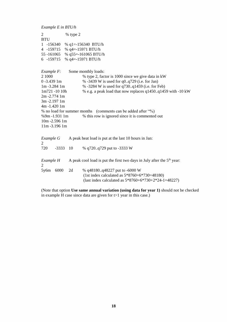
Example E in BTU/h

2 % type 2

BTU

1 -156340 % q1=-156340 BTU/h

4 -159715 % q4=-15971 BTU/h

55 -161065 % q55=-161065 BTU/h

6 -159715 % q4=-15971 BTU/h

Example F: Some monthly loads:

2 1000 % type 2, factor is 1000 since we give data in kW

0 -3.439 1m % -3439 W is used for q0..q729 (i.e. for Jan)

1m -3.284 1m % -3284 W is used for q730..q1459 (i.e. for Feb)

1m721 -10 10h % e.g. a peak load that now replaces q1450..q1459 with -10 kW

2m -2.774 1m

3m -2.197 1m

4m -1.420 1m

% no load for summer months (comments can be added after “%)

%9m -1.931 1m % this row is ignored since it is commented out

10m -2.596 1m

11m -3.196 1m

Example G A peak heat load is put at the last 10 hours in Jan:

2

720 -3333 10 % q720..q729 put to -3333 W

Example H A peak cool load is put the first two days in July after the 5th year:

2

5y6m 6000 2d % q48180..q48227 put to -6000 W

(1st index calculated as 5*8760+6*730=48180)

(last index calculated as 5*8760+6*730+2*24-1=48227)

(Note that option Use same annual variation (using data for year 1) should not be checked

in example H case since data are given for t>1 year in this case.)

19

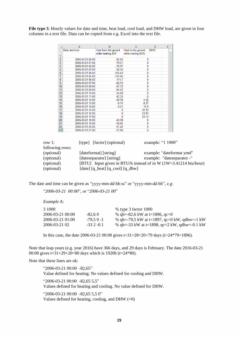
File type 3. Hourly values for date and time, heat load, cool load, and DHW load, are given in four

columns in a text file. Data can be copied from e.g. Excel into the text file.


following rows:

(optional) [dateformat] [string] example: "dateformat ymd"

(optional) [dateseparator] [string] example: "dateseparator -"


(optional) [date] [q_heat] [q_cool] [q_dhw]

The date and time can be given as “yyyy-mm-dd hh:ss” or “yyyy-mm-dd hh”, e.g:

“2006-03-21 00:00”, or “2006-03-21 00”

Example A:

3 1000 % type 3 factor 1000

2006-03-21 00:00 -82,6 0 % qh=-82,6 kW at t=1896, qc=0

2006-03-21 01:00 -79,5 0 -1 % qh=-79,5 kW at t=1897, qc=0 kW, qdhw=-1 kW

2006-03-21 02 -33 2 -0.1 % qh=-33 kW at t=1898, qc=2 kW, qdhw=-0.1 kW

In this case, the date 2006-03-21 00:00 gives t=31+28+20=79 days (t=24*79=1896).

Note that leap years (e.g. year 2016) have 366 days, and 29 days is February. The date 2016-03-21

00:00 gives t=31+29+20=80 days which is 1920h (t=24*80).

Note that these lines are ok:

“2006-03-21 00:00 -82,65”

Value defined for heating. No values defined for cooling and DHW.

“2006-03-21 00:00 -82,65 5,5”

Values defined for heating and cooling. No value defined for DHW.

“2006-03-21 00:00 -82,65 5,5 0”

Values defined for heating, cooling, and DHW (=0)

20

What does defined value means? Assume that "Make hourly loads from monthly base loads" and/or

"Make hourly loads from monthly peak loads" is checked. Defined values in files will always

override (exchange) the default values from monthly base and peak loads. If you do not want to

define a value use "x", such as

“2006-03-21 00:00 x 5,5 x” or just “2006-03-21 00:00 x 5,5”

Base load/peak load value will be used for heating and DHW, and 5,5 will be used for

cooling

“2006-03-21 00:00 82,65 x 0”

82,65 will be used for heating, base load/peak load value will be used for cooling, but value

will be zero for DHW

21

3.4 Date formats

Different date formats can be used in file type 1 and 3. The default date format is taken from the OS

settings. It is possible to force the format by using "dateformat" and "dateseparator", see examples

below.

It is sufficient to give "dateformat" and "dateseparator" once (before the first date is given).

Adding "dateformat" and "dateseparator" in a load file is recommended since the file will work on

all PC:s regardless of date formats in OS.

------------------------------------------------------------------------

Examples file type 1:

dateformat ymd % Sweden, Germany, etc

dateseparator -

date 2006-03-21 11:00

dateformat dmy % Germany, etc

dateseparator .

date 21.03.2006 11:00

dateformat mdy % USA, etc

dateseparator /

date 3/21/2006 11:00

------------------------------------------------------------------------

Example file type 3:

(Same input specified in three different date formats)

3 1000

dateformat ymd % Sweden, Germany, etc

dateseparator -

2006-03-21 00:00 -82,65 0 % (t=24*79=1896)

2006-03-21 01:00 -79,51 0 -1

2006-03-21 02 -33 2 -0.1

dateformat dmy % Germany, etc

dateseparator .

21.03.2006 00:00 -82,65 0 % (t=24*79=1896)

21.03.2006 01:00 -79,51 0 -1

21.03.2006 02 -33 2 -0.1

dateformat mdy % USA, etc

dateseparator /

03/21/2006 00:00 -82,65 0 % (t=24*79=1896)

03/21/2006 01:00 -79,51 0 -1

03/21/2006 02 -33 2 -0.1

22

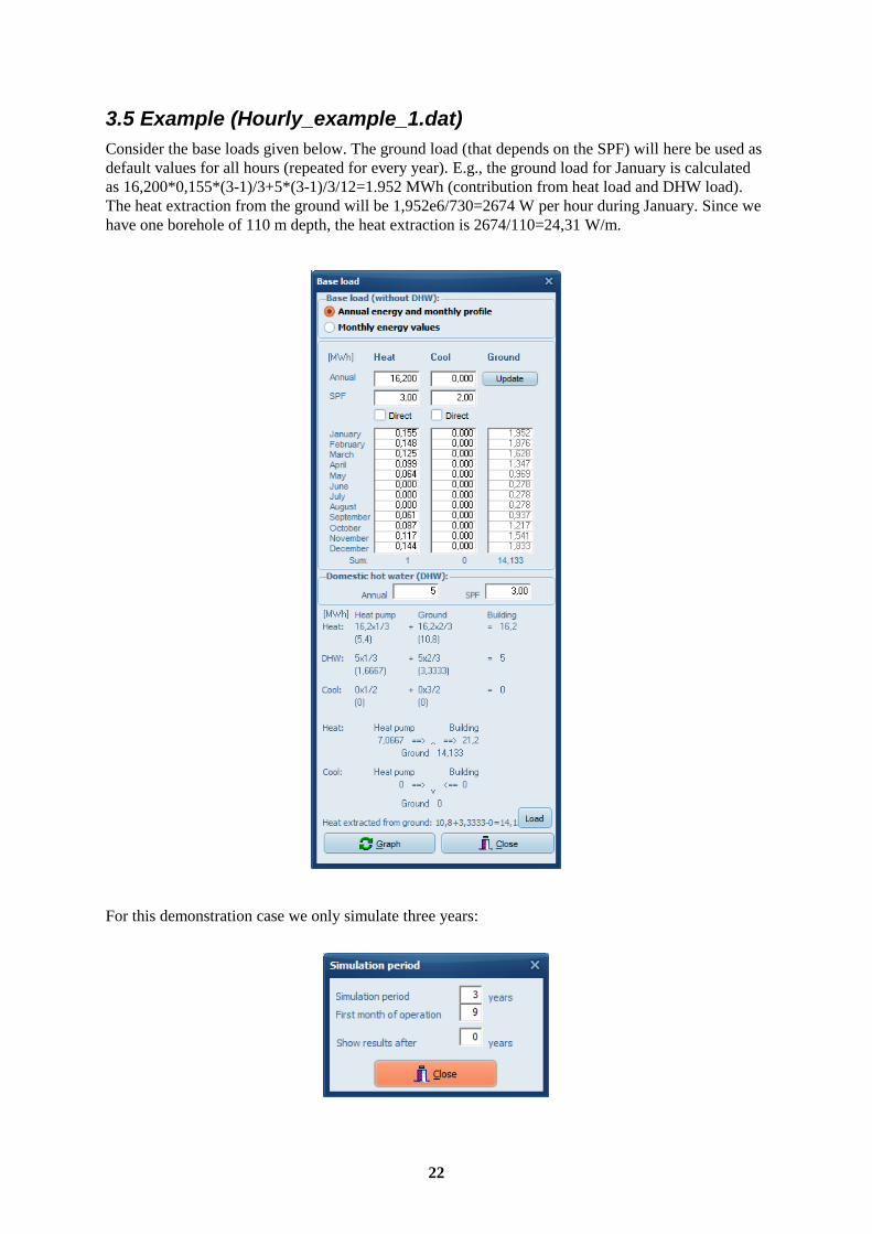
3.5 Example (Hourly_example_1.dat)

Consider the base loads given below. The ground load (that depends on the SPF) will here be used as

default values for all hours (repeated for every year). E.g., the ground load for January is calculated

as 16,200*0,155*(3-1)/3+5*(3-1)/3/12=1.952 MWh (contribution from heat load and DHW load).

The heat extraction from the ground will be 1,952e6/730=2674 W per hour during January. Since we

have one borehole of 110 m depth, the heat extraction is 2674/110=24,31 W/m.

For this demonstration case we only simulate three years:

23

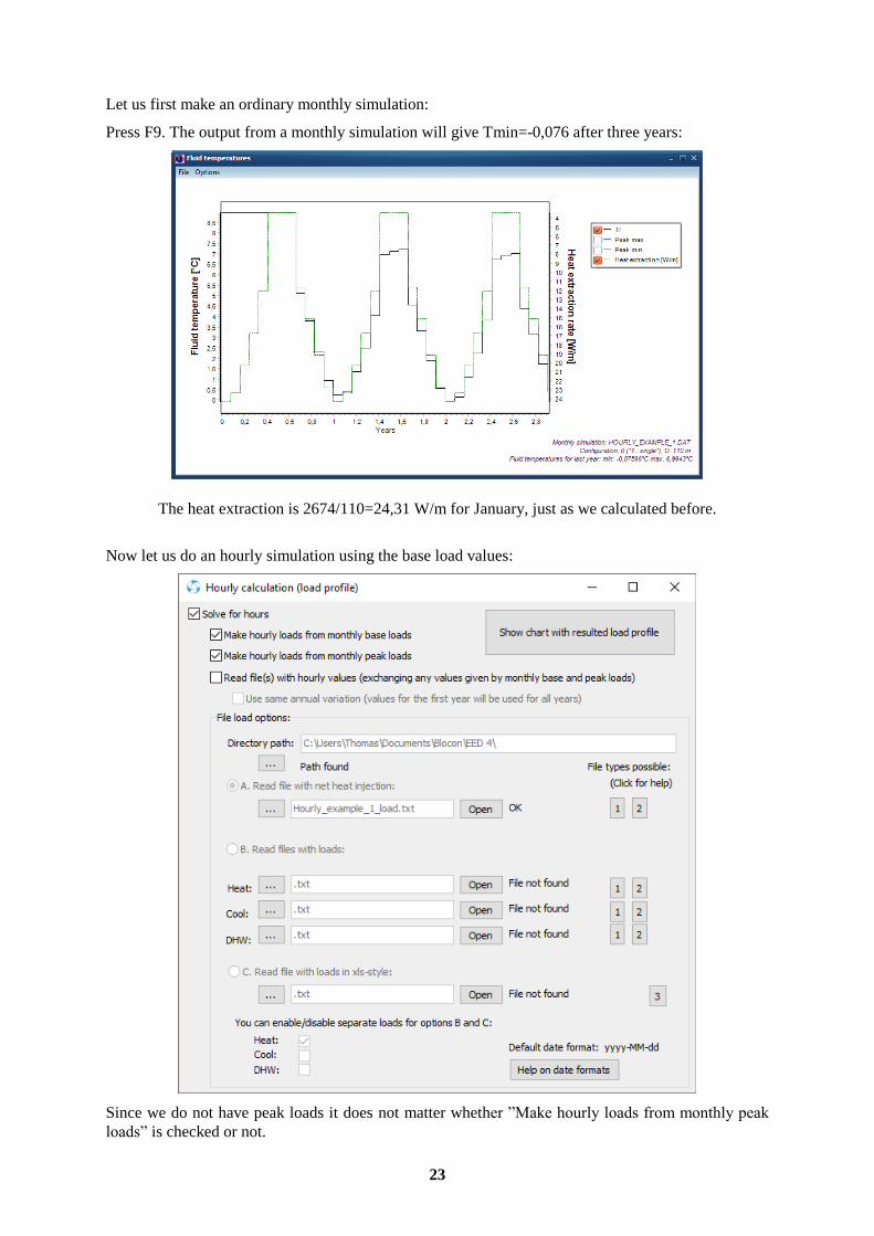
Let us first make an ordinary monthly simulation:

Press F9. The output from a monthly simulation will give Tmin=-0,076 after three years:

The heat extraction is 2674/110=24,31 W/m for January, just as we calculated before.

Now let us do an hourly simulation using the base load values:

Since we do not have peak loads it does not matter whether ”Make hourly loads from monthly peak

loads” is checked or not.

24

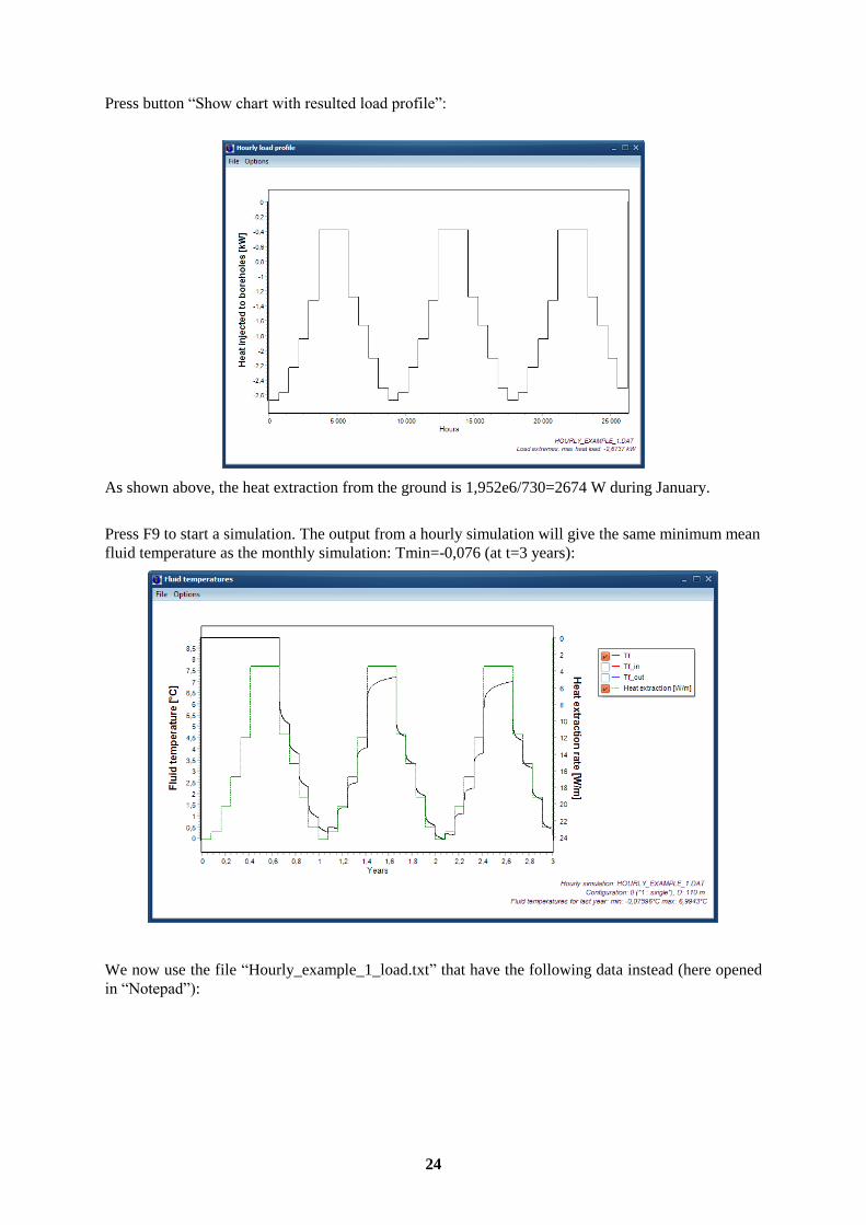
Press button “Show chart with resulted load profile”:

As shown above, the heat extraction from the ground is 1,952e6/730=2674 W during January.

Press F9 to start a simulation. The output from a hourly simulation will give the same minimum mean

fluid temperature as the monthly simulation: Tmin=-0,076 (at t=3 years):

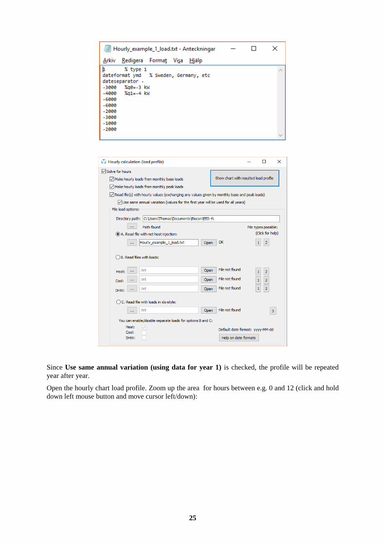
We now use the file “Hourly_example_1_load.txt” that have the following data instead (here opened

in “Notepad”):

25

Since Use same annual variation (using data for year 1) is checked, the profile will be repeated

year after year.

Open the hourly chart load profile. Zoom up the area for hours between e.g. 0 and 12 (click and hold

down left mouse button and move cursor left/down):

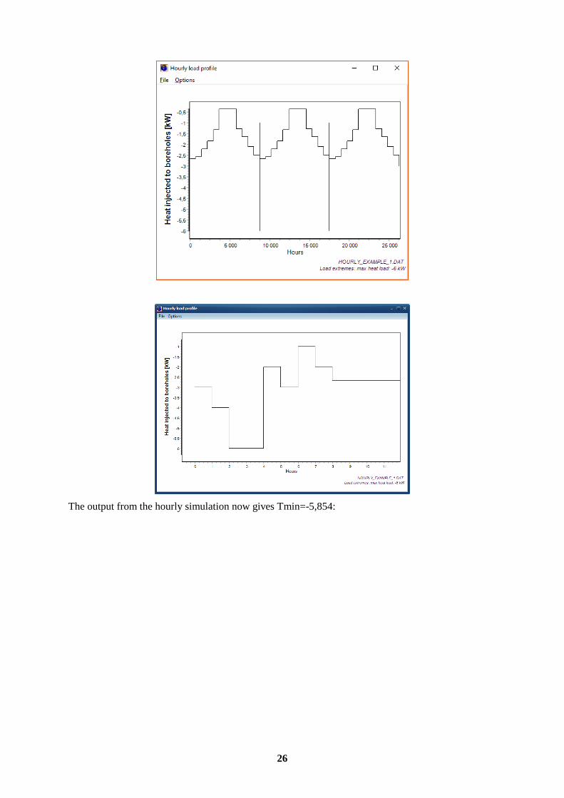
26

The output from the hourly simulation now gives Tmin=-5,854:

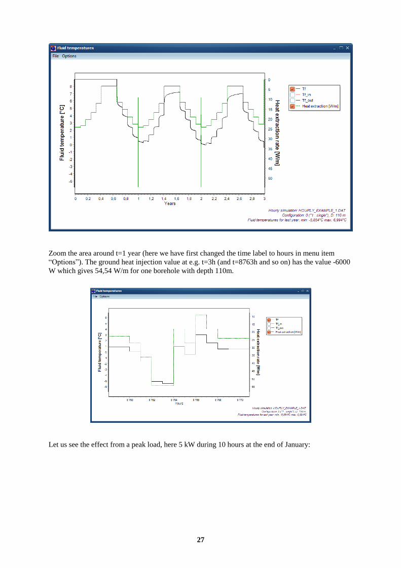
27

Zoom the area around t=1 year (here we have first changed the time label to hours in menu item

“Options”). The ground heat injection value at e.g. t=3h (and t=8763h and so on) has the value -6000

W which gives 54,54 W/m for one borehole with depth 110m.

Let us see the effect from a peak load, here 5 kW during 10 hours at the end of January:

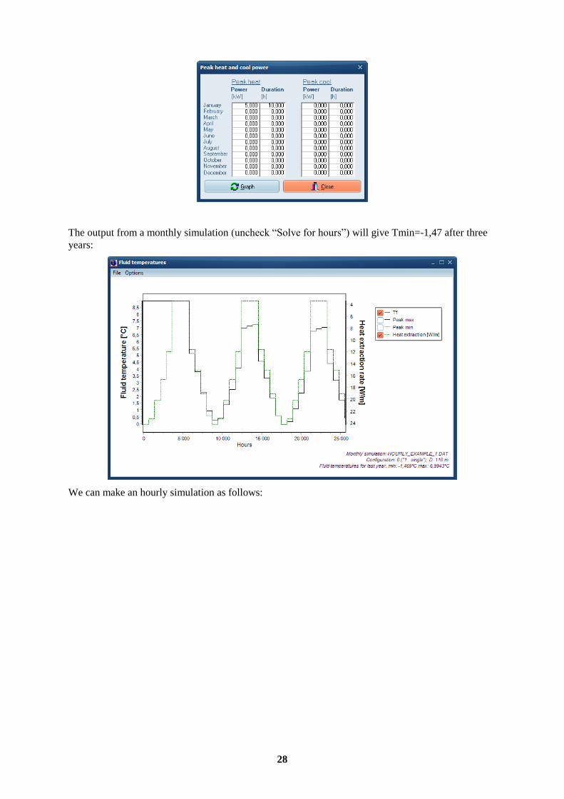
28

The output from a monthly simulation (uncheck “Solve for hours”) will give Tmin=-1,47 after three

years:

We can make an hourly simulation as follows:

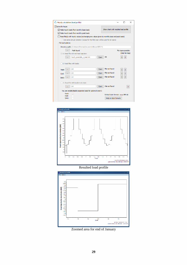
29

Resulted load profile

Zoomed area for end of January

30

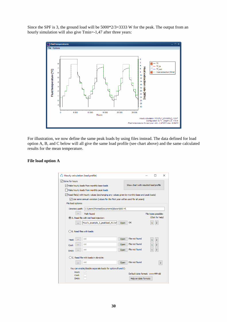
Since the SPF is 3, the ground load will be 5000*2/3=3333 W for the peak. The output from an

hourly simulation will also give Tmin=-1,47 after three years:

For illustration, we now define the same peak loads by using files instead. The data defined for load

option A, B, and C below will all give the same load profile (see chart above) and the same calculated

results for the mean temperature.

File load option A

31

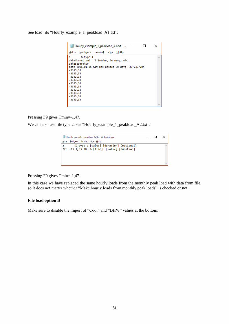
See load file “Hourly_example_1_peakload_A1.txt”:

Pressing F9 gives Tmin=-1,47.

We can also use file type 2, see “Hourly_example_1_peakload_A2.txt”.


In this case we have replaced the same hourly loads from the monthly peak load with data from file,

so it does not matter whether “Make hourly loads from monthly peak loads” is checked or not,

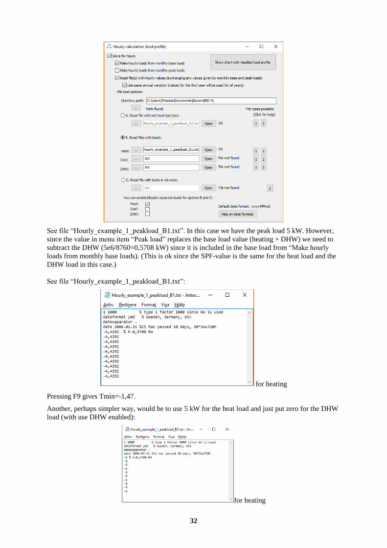
File load option B

Make sure to disable the import of “Cool” and “DHW” values at the bottom:

32

See file “Hourly_example_1_peakload_B1.txt”. In this case we have the peak load 5 kW. However,

since the value in menu item “Peak load” replaces the base load value (heating + DHW) we need to

subtract the DHW (5e6/8760=0,5708 kW) since it is included in the base load from “Make hourly

loads from monthly base loads). (This is ok since the SPF-value is the same for the heat load and the

DHW load in this case.)

See file “Hourly_example_1_peakload_B1.txt”:

for heating


Another, perhaps simpler way, would be to use 5 kW for the heat load and just put zero for the DHW

load (with use DHW enabled):

for heating

33

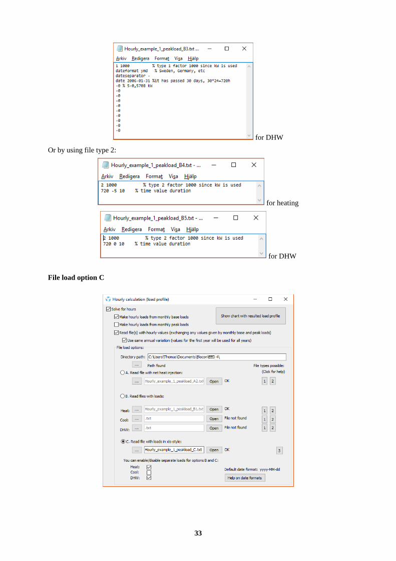
for DHW

Or by using file type 2:

for heating

for DHW

File load option C

34

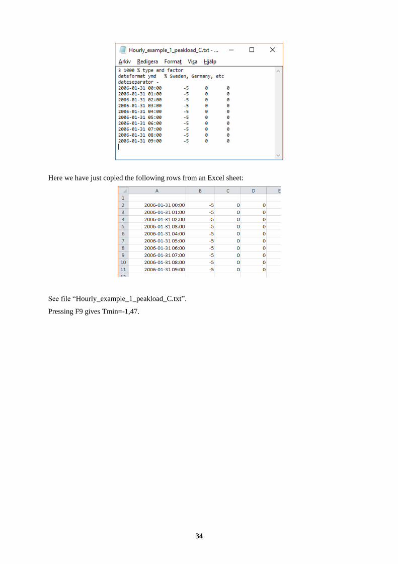
Here we have just copied the following rows from an Excel sheet:

See file “Hourly_example_1_peakload_C.txt”.


35

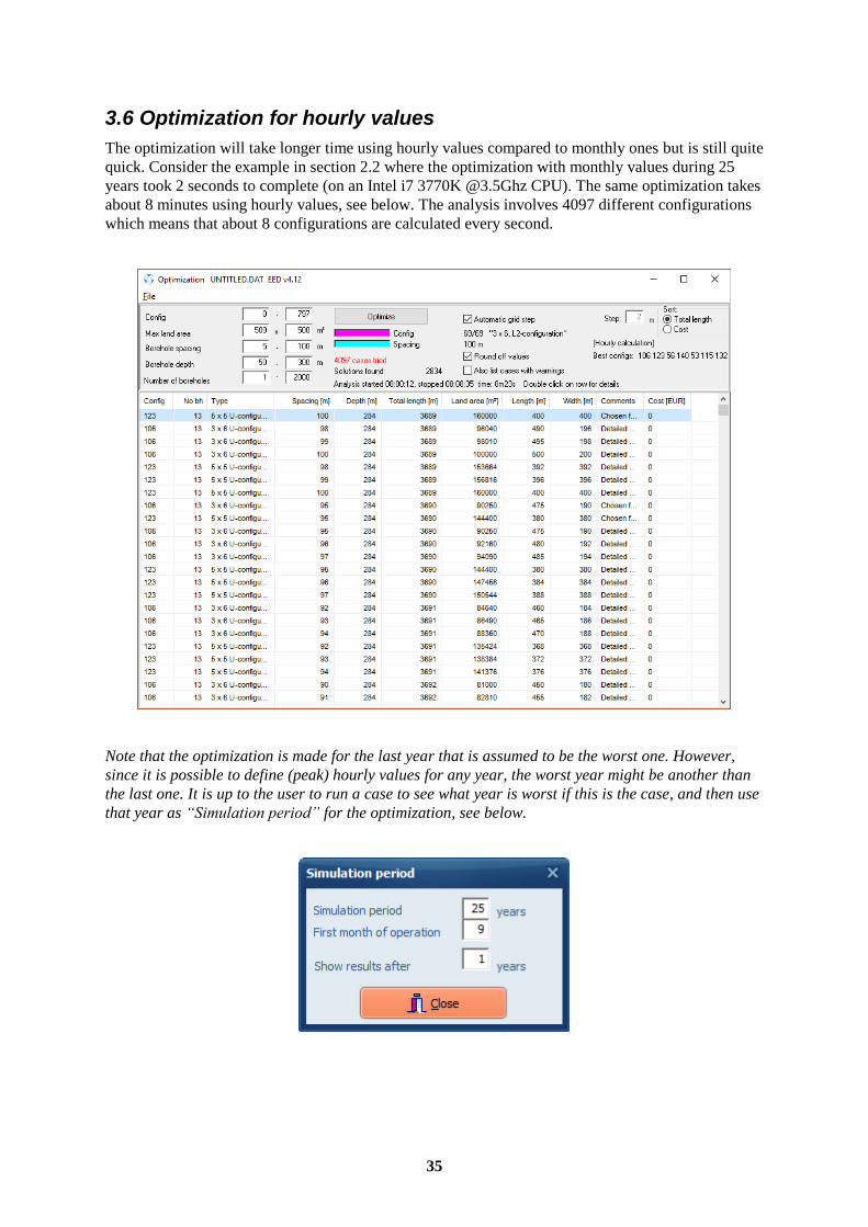
3.6 Optimization for hourly values

The optimization will take longer time using hourly values compared to monthly ones but is still quite

quick. Consider the example in section 2.2 where the optimization with monthly values during 25

years took 2 seconds to complete (on an Intel i7 3770K @3.5Ghz CPU). The same optimization takes

about 8 minutes using hourly values, see below. The analysis involves 4097 different configurations

which means that about 8 configurations are calculated every second.

Note that the optimization is made for the last year that is assumed to be the worst one. However,

since it is possible to define (peak) hourly values for any year, the worst year might be another than

the last one. It is up to the user to run a case to see what year is worst if this is the case, and then use

that year as “Simulation period” for the optimization, see below.

36

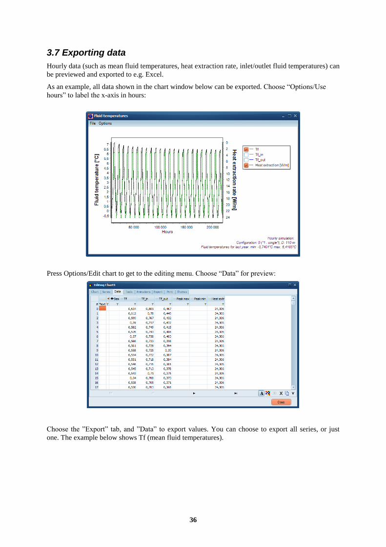
3.7 Exporting data

Hourly data (such as mean fluid temperatures, heat extraction rate, inlet/outlet fluid temperatures) can

be previewed and exported to e.g. Excel.

As an example, all data shown in the chart window below can be exported. Choose “Options/Use

hours” to label the x-axis in hours:

Press Options/Edit chart to get to the editing menu. Choose “Data” for preview:

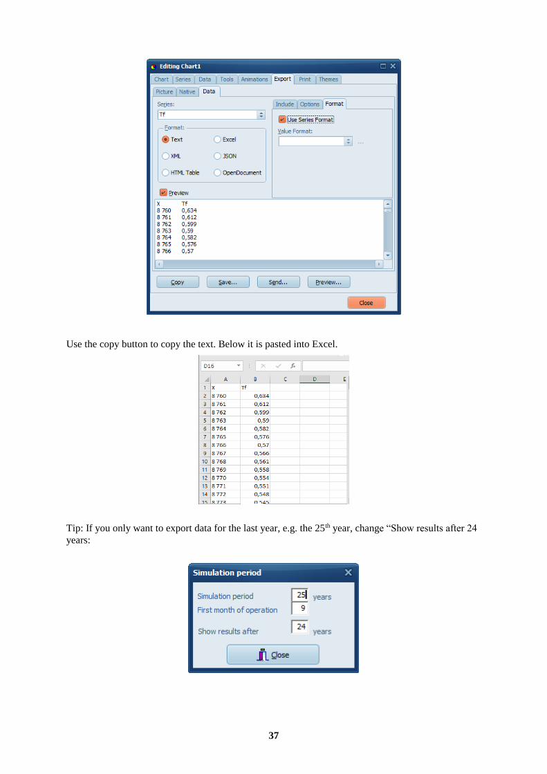
Choose the ”Export” tab, and ”Data” to export values. You can choose to export all series, or just

one. The example below shows Tf (mean fluid temperatures).

37

Use the copy button to copy the text. Below it is pasted into Excel.

Tip: If you only want to export data for the last year, e.g. the 25th year, change “Show results after 24

years:

38

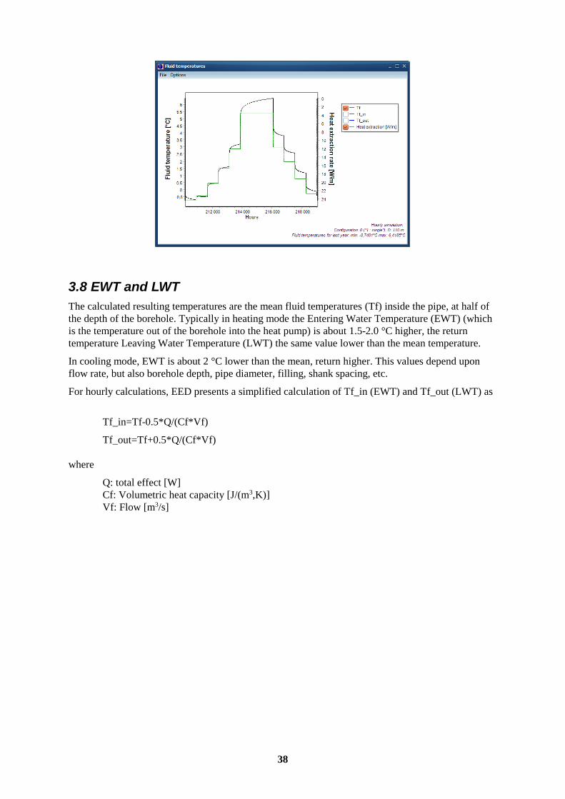
3.8 EWT and LWT

The calculated resulting temperatures are the mean fluid temperatures (Tf) inside the pipe, at half of

the depth of the borehole. Typically in heating mode the Entering Water Temperature (EWT) (which

is the temperature out of the borehole into the heat pump) is about 1.5-2.0 °C higher, the return

temperature Leaving Water Temperature (LWT) the same value lower than the mean temperature.

In cooling mode, EWT is about 2 °C lower than the mean, return higher. This values depend upon

flow rate, but also borehole depth, pipe diameter, filling, shank spacing, etc.

For hourly calculations, EED presents a simplified calculation of Tf_in (EWT) and Tf_out (LWT) as

Tf_in=Tf-0.5*Q/(Cf*Vf)

Tf_out=Tf+0.5*Q/(Cf*Vf)

where

Q: total effect [W]

Cf: Volumetric heat capacity [J/(m3,K)]

Vf: Flow [m3/s]

39

4. Approximation for irregular configurations [Updated in v4.14]

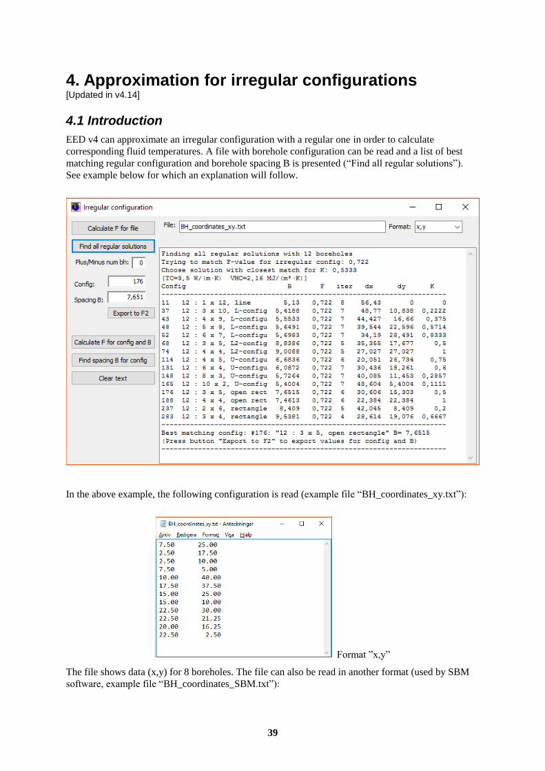
4.1 Introduction

EED v4 can approximate an irregular configuration with a regular one in order to calculate

corresponding fluid temperatures. A file with borehole configuration can be read and a list of best

matching regular configuration and borehole spacing B is presented (“Find all regular solutions”).

See example below for which an explanation will follow.

In the above example, the following configuration is read (example file “BH_coordinates_xy.txt”):

Format ”x,y”

The file shows data (x,y) for 8 boreholes. The file can also be read in another format (used by SBM

software, example file “BH_coordinates_SBM.txt”):

40

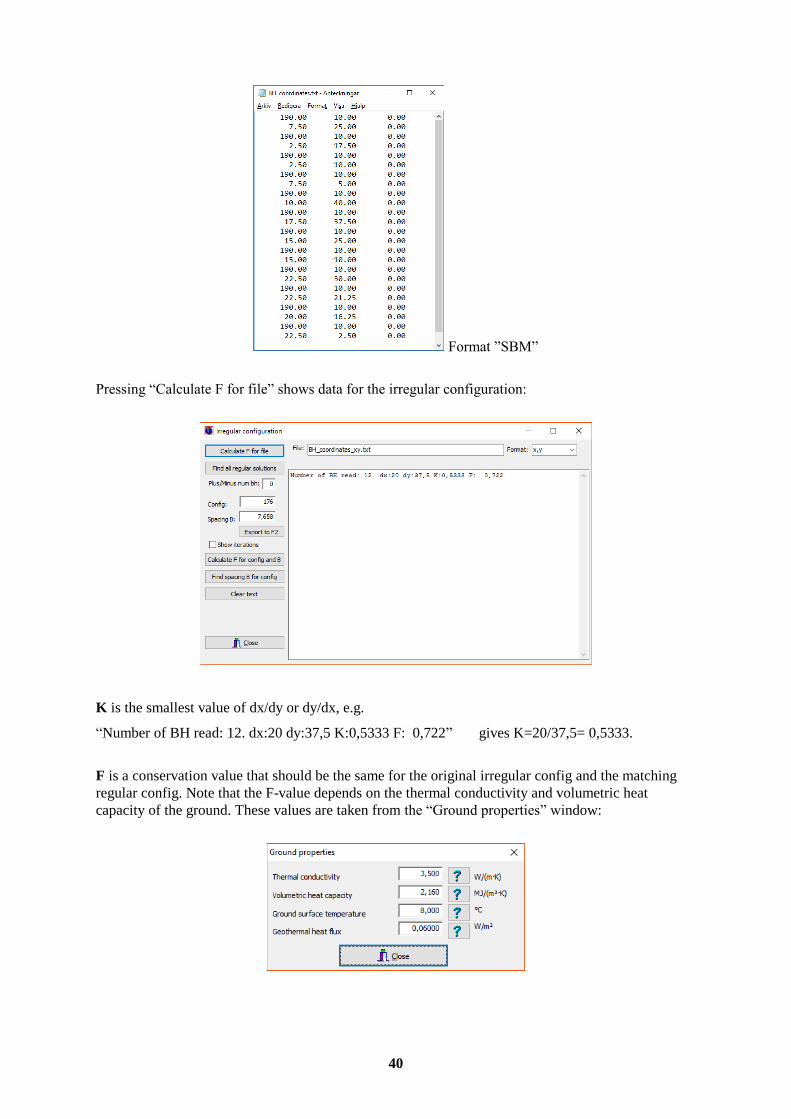
Format ”SBM”

Pressing “Calculate F for file” shows data for the irregular configuration:

K is the smallest value of dx/dy or dy/dx, e.g.

“Number of BH read: 12. dx:20 dy:37,5 K:0,5333 F: 0,722” gives K=20/37,5= 0,5333.

F is a conservation value that should be the same for the original irregular config and the matching

regular config. Note that the F-value depends on the thermal conductivity and volumetric heat

capacity of the ground. These values are taken from the “Ground properties” window:

41

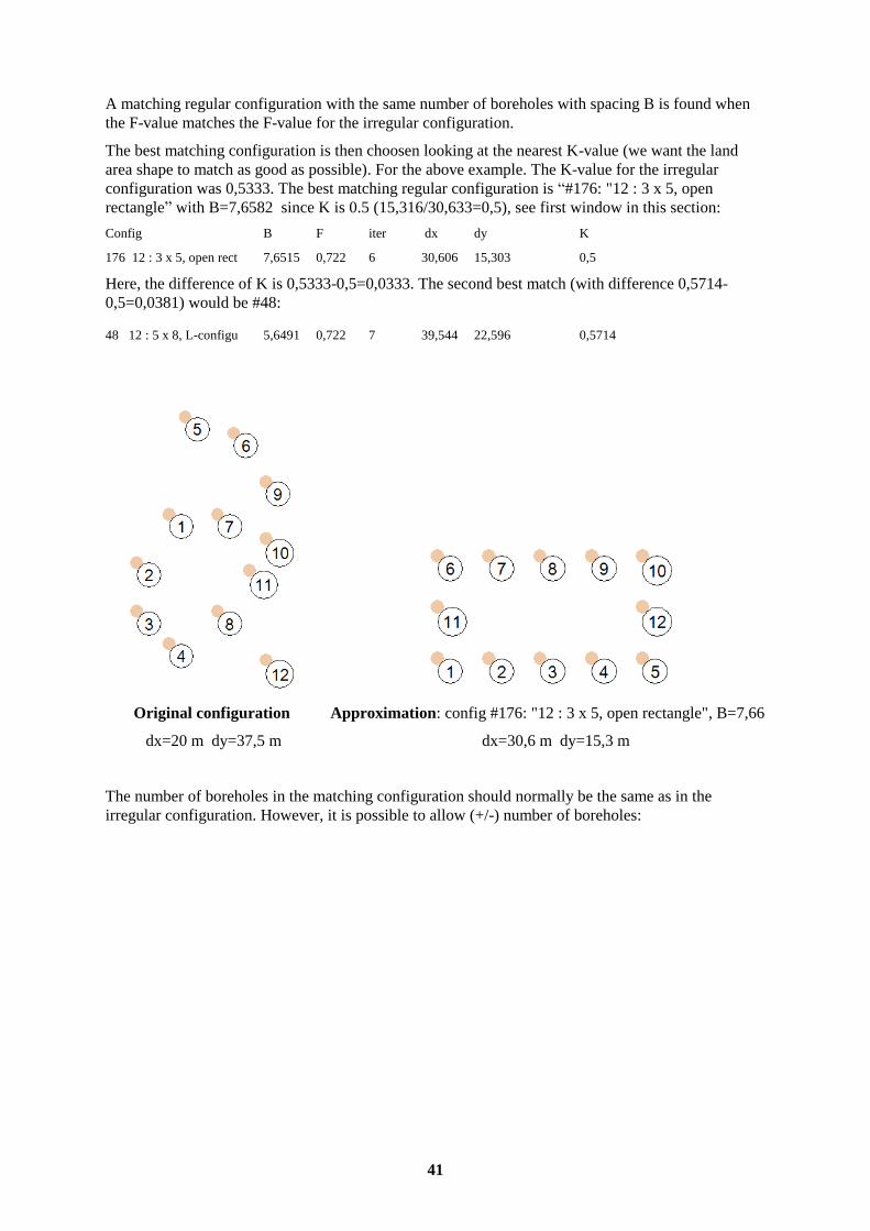
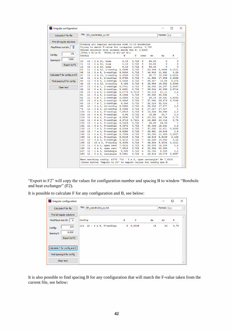
A matching regular configuration with the same number of boreholes with spacing B is found when

the F-value matches the F-value for the irregular configuration.

The best matching configuration is then choosen looking at the nearest K-value (we want the land

area shape to match as good as possible). For the above example. The K-value for the irregular

configuration was 0,5333. The best matching regular configuration is “#176: "12 : 3 x 5, open

rectangle” with B=7,6582 since K is 0.5 (15,316/30,633=0,5), see first window in this section:

Config B F iter dx dy K

176 12 : 3 x 5, open rect 7,6515 0,722 6 30,606 15,303 0,5

Here, the difference of K is 0,5333-0,5=0,0333. The second best match (with difference 0,5714-

0,5=0,0381) would be #48:

48 12 : 5 x 8, L-configu 5,6491 0,722 7 39,544 22,596 0,5714

Original configuration Approximation: config #176: "12 : 3 x 5, open rectangle", B=7,66

dx=20 m dy=37,5 m dx=30,6 m dy=15,3 m

The number of boreholes in the matching configuration should normally be the same as in the

irregular configuration. However, it is possible to allow (+/-) number of boreholes:

42

“Export to F2” will copy the values for configuration number and spacing B to window “Borehole

and heat exchanger” (F2).

It is possible to calculate F for any configuration and B, see below:

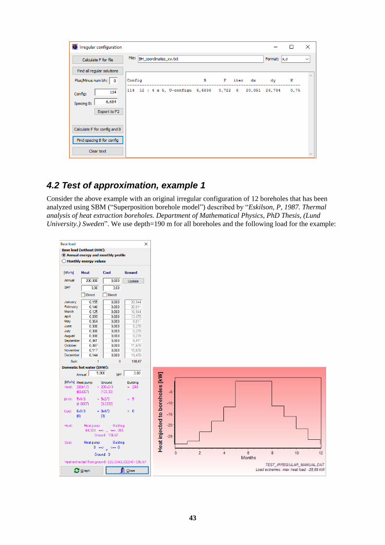
It is also possible to find spacing B for any configuration that will match the F-value taken from the

current file, see below:

43

4.2 Test of approximation, example 1

Consider the above example with an original irregular configuration of 12 boreholes that has been

analyzed using SBM (“Superposition borehole model”) described by “Eskilson, P, 1987. Thermal

analysis of heat extraction boreholes. Department of Mathematical Physics, PhD Thesis, (Lund

University.) Sweden”. We use depth=190 m for all boreholes and the following load for the example:

44

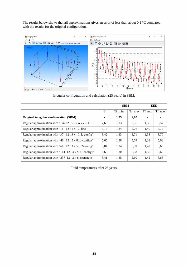
The results below shows that all approximations gives an error of less than about 0.1 °C compared

with the results for the original configuration.

Irregular configuration and calculation (25 years) in SBM.

SBM EED

B Tf_min Tf_max Tf_min Tf_max

Original irregular configuration (SBM) - 1,39 5,62 - -

Regular approximation with “176 12 : 3 x 5, open rect” 7,65 1,33 5,55 1,35 5,57

Regular approximation with “11 12 : 1 x 12, line” 5,13 1,34 5,76 1,40 5,75

Regular approximation with “37 12 : 3 x 10, L-config” 5,42 1,33 5,71 1,38 5,70

Regular approximation with “48 12 : 5 x 8, L-configu” 5,65 1,38 5,69 1,39 5,68

Regular approximation with “68 12 : 3 x 5, L2-config” 8,84 1,34 5,59 1,42 5,60

Regular approximation with “114 12 : 4 x 5, U-configu” 6,68 1,30 5,58 1,35 5,60

Regular approximation with “237 12 : 2 x 6, rectangle” 8,41 1,35 5,60 1,42 5,63

Fluid temperatures after 25 years.

45

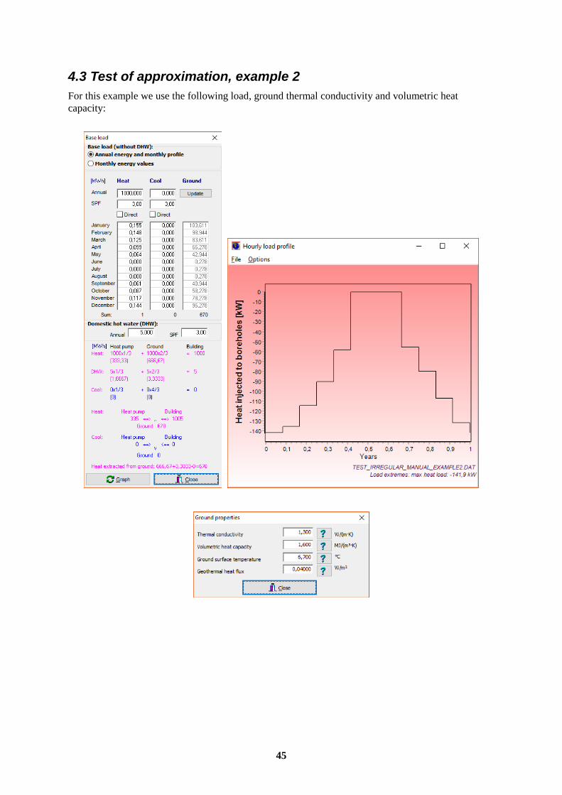
4.3 Test of approximation, example 2

For this example we use the following load, ground thermal conductivity and volumetric heat

capacity:

46

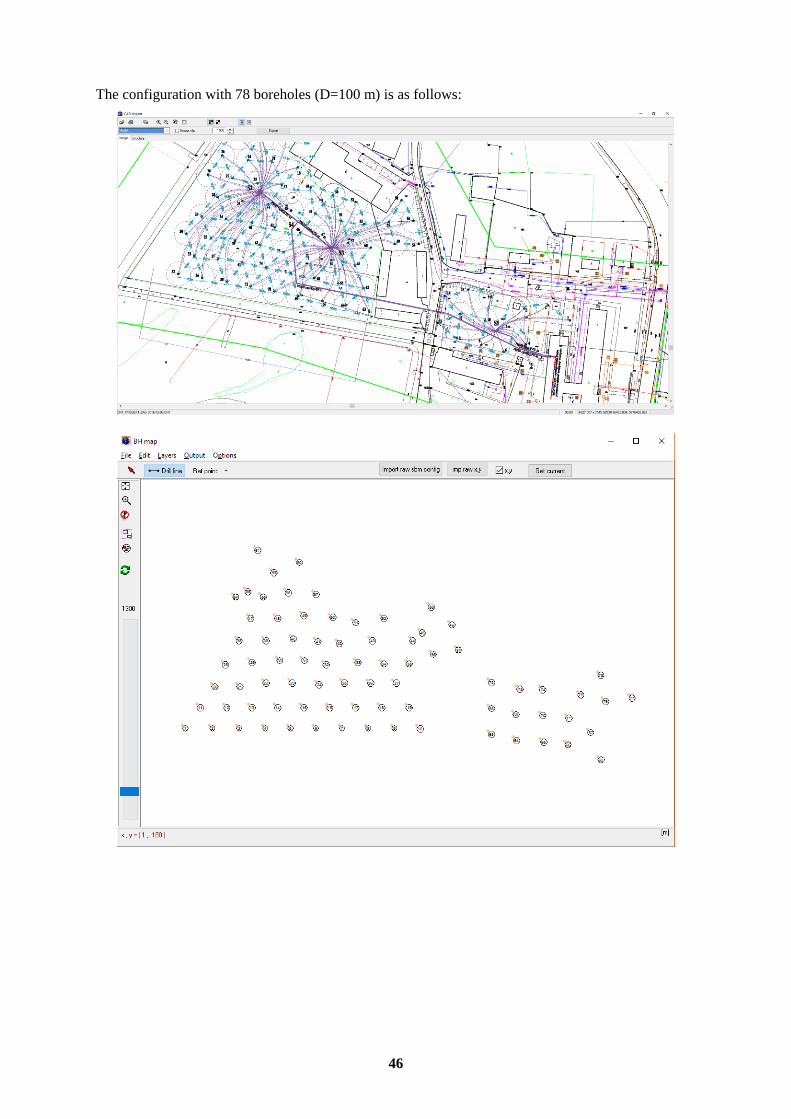
The configuration with 78 boreholes (D=100 m) is as follows:

47

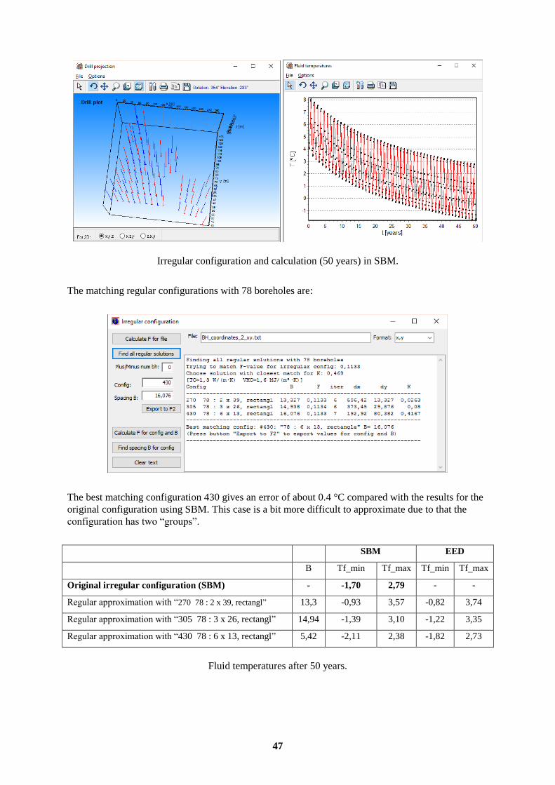
Irregular configuration and calculation (50 years) in SBM.

The matching regular configurations with 78 boreholes are:

The best matching configuration 430 gives an error of about 0.4 °C compared with the results for the

original configuration using SBM. This case is a bit more difficult to approximate due to that the

configuration has two “groups”.

SBM EED

B Tf_min Tf_max Tf_min Tf_max

Original irregular configuration (SBM) - -1,70 2,79 - -

Regular approximation with “270 78 : 2 x 39, rectangl” 13,3 -0,93 3,57 -0,82 3,74



Fluid temperatures after 50 years.

48

5. Changeable user interface of EED

5.1 Introduction

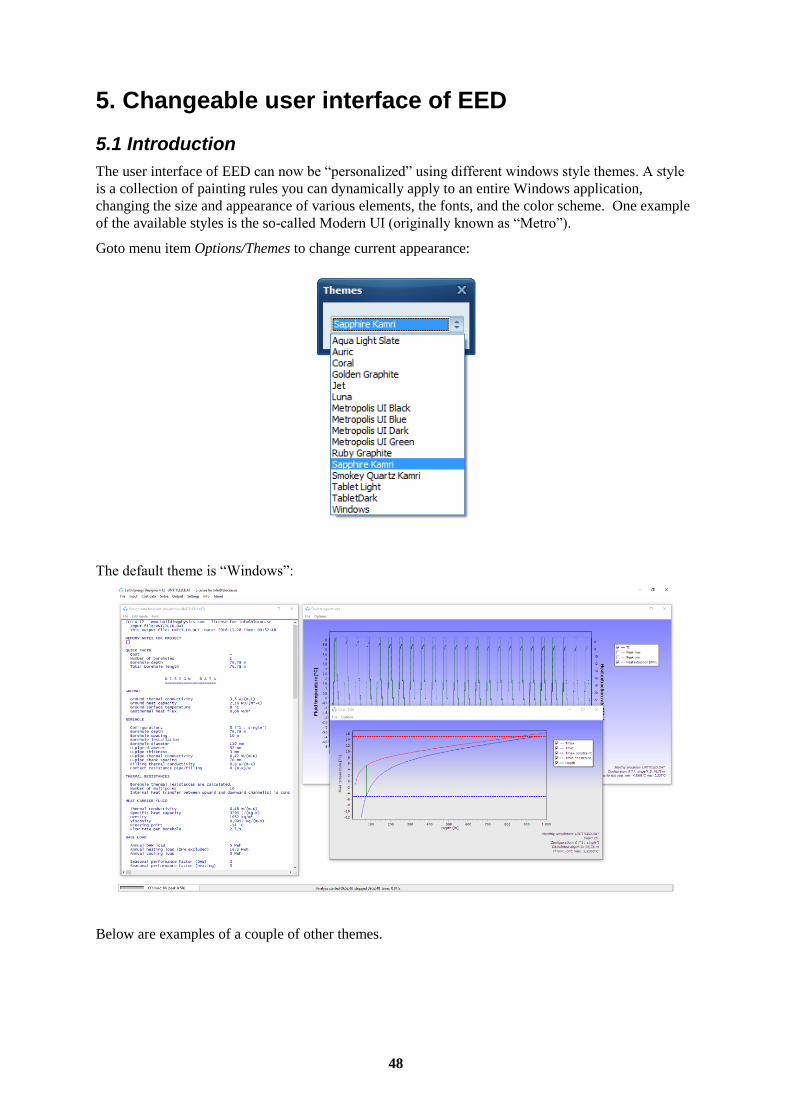
The user interface of EED can now be “personalized” using different windows style themes. A style

is a collection of painting rules you can dynamically apply to an entire Windows application,

changing the size and appearance of various elements, the fonts, and the color scheme. One example

of the available styles is the so-called Modern UI (originally known as “Metro”).

Goto menu item Options/Themes to change current appearance:

The default theme is “Windows”:

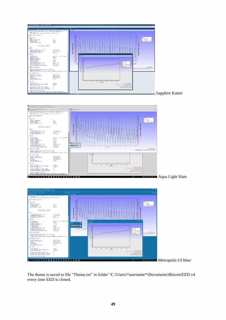
Below are examples of a couple of other themes.

49

Sapphire Kamri

Aqua Light Slate

Metropolis UI blue:

The theme is saved to file “Theme.txt” in folder “C:\Users\*username*\Documents\Blocon\EED v4

every time EED is closed.

50

6. Faster hourly simulations [Available in v4.14]

6.1 Introduction

Hourly simulations of borehole fluid temperatures are time consuming. There are several methods

reported in literature that decreases the calculation time by using so-called load aggregation schemes

that lump the hourly loads on a borehole heat exchanger into larger blocks of time in order to reduce

the number of operations needed. One example is shown in “A load-aggregation method to calculate

extraction temperatures of borehole heat exchangers” [1], see

http://publications.lib.chalmers.se/records/fulltext/163661/local_163661.pdf

EED v4.14 uses a different approach that is very fast (and does not introduce an error as in the load

aggregation case). Solving 25 years of hourly fluid temperatures takes less than a second on a hi-end

CPU, and only a few seconds when solving for 100 years.

This impressive speed is due to the capabilities of modern CPU:s. The calculation of fluid

temperatures using the g-function is well suited for multiple CPU processing that performs the same

operation on multiple data points simultaneously. This method is sometimes called “single

instruction, multiple data” (SIMD), see e.g.

https://en.wikipedia.org/wiki/SIMD

Instead of using traditional (“serial”) programming where floating point operations are performed on

an element in a vector one by one, modern CPU:s can make these calculations for the whole vector at

the same time. In addition to this, most modern computers have multiple cores that will accelerate the

calculation speed even further (roughly speaking; if we e.g. have a PC with 4 cores we can do

calculations for 4 different hours at the same time). The total speed gain is typically 10-150 times

higher compared to using conventional serial implementation. The higher number of cores, the faster

speed increase.

As described above, EED can use the CPU (“central processing unit”) for fast SIMD calculations. As

an alternative, EED can also use the GPU (“graphics processing unit”) to speed up calculations.

Architecturally, a CPU is composed of just a few cores that can handle a few software threads at a

time. In contrast, a GPU is composed of hundreds, or thousands, of cores that can handle thousands

of threads simultaneously. Also, the GPU achieves this acceleration while often being more power-

and cost-efficient than a CPU. The gain using a hi-end graphics card (GPU) might be 200-300 times.

In the benchmarks below, one example shows that it is possible to solve for 100 years in just 4

seconds on a $300 graphics card (Radeon RX 480).

EED can uses GPU:s (and other devices) that are conformant with OpenCL, see

https://en.wikipedia.org/wiki/OpenCL

For OpenCL compliant devices (such as graphics cards), see

https://www.khronos.org/conformance/adopters/conformant-products#opencl

EED uses the CPU as the default choice since many graphics cards (GPU:s) are not compatible. It is

up to the user to test the GPU method.

References:

[1] Claesson, J, Javed, S, 2012. A load-aggregation method to calculate extraction temperatures of

borehole heat exchangers. ASHRAE Transactions, vol. 118(1), pp. 530-539.

http://publications.lib.chalmers.se/records/fulltext/163661/local_163661.pdf

https://en.wikipedia.org/wiki/SIMD

https://en.wikipedia.org/wiki/OpenCL

https://www.khronos.org/conformance/adopters/conformant-products#opencl

51

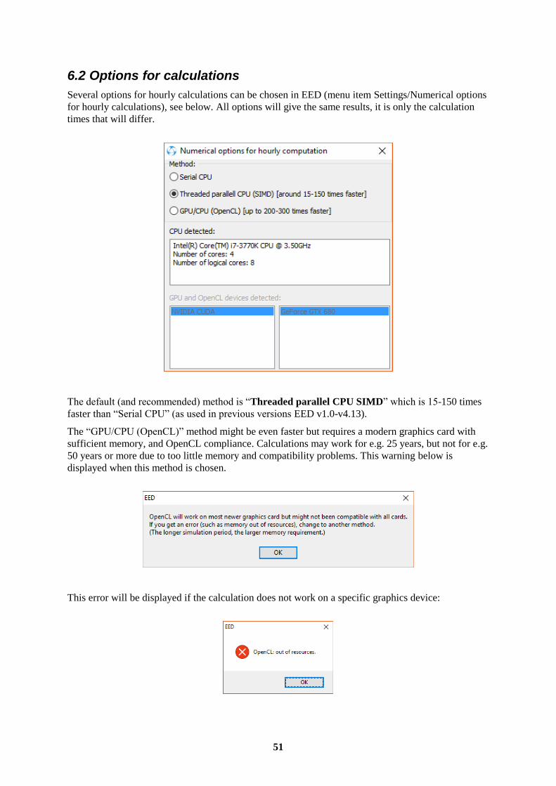
6.2 Options for calculations

Several options for hourly calculations can be chosen in EED (menu item Settings/Numerical options

for hourly calculations), see below. All options will give the same results, it is only the calculation

times that will differ.

The default (and recommended) method is “Threaded parallel CPU SIMD” which is 15-150 times

faster than “Serial CPU” (as used in previous versions EED v1.0-v4.13).

The “GPU/CPU (OpenCL)” method might be even faster but requires a modern graphics card with

sufficient memory, and OpenCL compliance. Calculations may work for e.g. 25 years, but not for e.g.

50 years or more due to too little memory and compatibility problems. This warning below is

displayed when this method is chosen.

This error will be displayed if the calculation does not work on a specific graphics device:

52

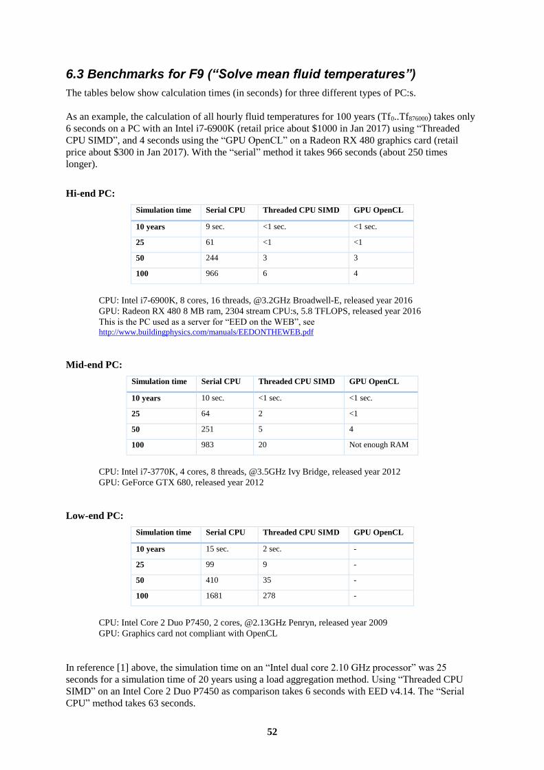
6.3 Benchmarks for F9 (“Solve mean fluid temperatures”)

The tables below show calculation times (in seconds) for three different types of PC:s.

As an example, the calculation of all hourly fluid temperatures for 100 years (Tf0..Tf876000) takes only

6 seconds on a PC with an Intel i7-6900K (retail price about $1000 in Jan 2017) using “Threaded

CPU SIMD”, and 4 seconds using the “GPU OpenCL” on a Radeon RX 480 graphics card (retail

price about $300 in Jan 2017). With the “serial” method it takes 966 seconds (about 250 times

longer).

Hi-end PC:

Simulation time Serial CPU Threaded CPU SIMD GPU OpenCL

10 years 9 sec. <1 sec. <1 sec.

25 61 <1 <1

50 244 3 3

100 966 6 4

CPU: Intel i7-6900K, 8 cores, 16 threads, @3.2GHz Broadwell-E, released year 2016

GPU: Radeon RX 480 8 MB ram, 2304 stream CPU:s, 5.8 TFLOPS, released year 2016

This is the PC used as a server for “EED on the WEB”, see http://www.buildingphysics.com/manuals/EEDONTHEWEB.pdf

Mid-end PC:


10 years 10 sec. <1 sec. <1 sec.

25 64 2 <1

50 251 5 4

100 983 20 Not enough RAM

CPU: Intel i7-3770K, 4 cores, 8 threads, @3.5GHz Ivy Bridge, released year 2012

GPU: GeForce GTX 680, released year 2012

Low-end PC:


10 years 15 sec. 2 sec. -

25 99 9 -

50 410 35 -

100 1681 278 -

CPU: Intel Core 2 Duo P7450, 2 cores, @2.13GHz Penryn, released year 2009

GPU: Graphics card not compliant with OpenCL

In reference [1] above, the simulation time on an “Intel dual core 2.10 GHz processor” was 25

seconds for a simulation time of 20 years using a load aggregation method. Using “Threaded CPU

SIMD” on an Intel Core 2 Duo P7450 as comparison takes 6 seconds with EED v4.14. The “Serial

CPU” method takes 63 seconds.


53

It should be noted that the speed increase between e.g. “Threaded CPU SIMD” and “Serial CPU” is

higher for newer PC:s (due to newer SIMD options and higher number of cores), such as on i3-, i5-,

and i7-CPU:s.

6.4 Benchmarks for F10 (“Solve required borehole length”)

For this calculation, the “Threaded CPU SIMD” will always be used unless “Serial CPU” is chosen.

Note that the serial method also has been improved in v4.14.

Simulation time Serial CPU

v4.13

Serial CPU

v4.14

Threaded CPU SIMD

v4.14

GPU OpenCL

10 years 5 sec. 4 sec. 2 sec.

“Threaded CPU SIMD”

will be used for all calculations 25 11 8 3

50 22 15 7

100 43 29 19

CPU: Intel i7-3770K, 4 Cores, 8 Threads, @3.5GHz Ivy Bridge (released year 2012)

GPU: GeForce GTX 680 (released year 2012)

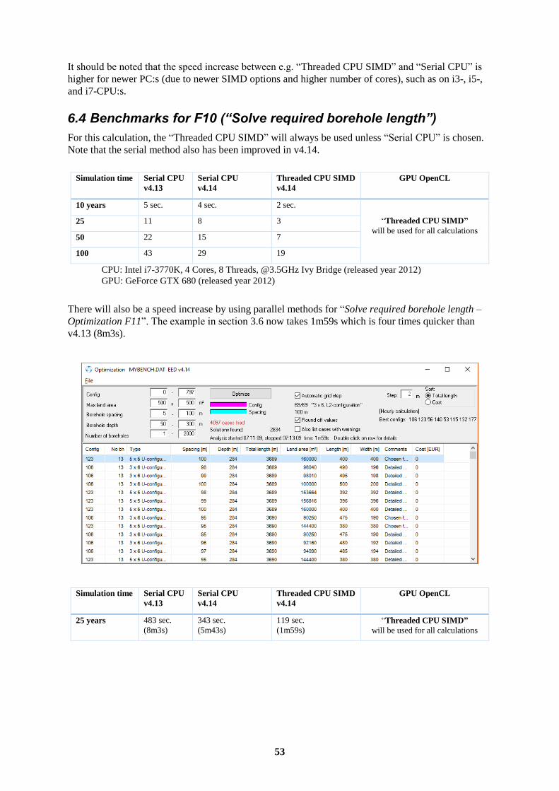
There will also be a speed increase by using parallel methods for “Solve required borehole length –

Optimization F11”. The example in section 3.6 now takes 1m59s which is four times quicker than

v4.13 (8m3s).

Simulation time Serial CPU

v4.13

Serial CPU

v4.14

Threaded CPU SIMD

v4.14

GPU OpenCL

25 years 483 sec.

(8m3s)

343 sec.

(5m43s)

119 sec.

(1m59s)

“Threaded CPU SIMD”

will be used for all calculations

54

Appendix A. List of new update features For update info, see also http://www.buildingphysics.com/index-filer/Page1139.htm

Update 4.14 (Jan 4, 2017)

Faster hourly simulations. See Chapter 6.

Approximation for irregular configurations. Updated solver. See Chapter 4.

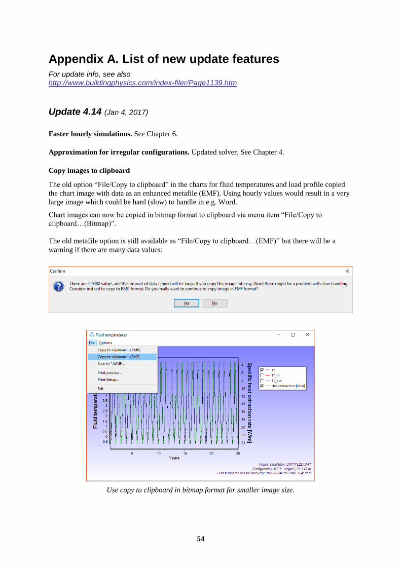
Copy images to clipboard

The old option “File/Copy to clipboard” in the charts for fluid temperatures and load profile copied

the chart image with data as an enhanced metafile (EMF). Using hourly values would result in a very

large image which could be hard (slow) to handle in e.g. Word.

Chart images can now be copied in bitmap format to clipboard via menu item “File/Copy to

clipboard…(Bitmap)”.

The old metafile option is still available as “File/Copy to clipboard…(EMF)” but there will be a

warning if there are many data values:

Use copy to clipboard in bitmap format for smaller image size.


55

Date format

Dates can now be written in short format in the xls-style option, e.g. as for a German date type:

“1.9.2015 4 -18,6 0,0 0” (short format “m.d.yyyy h is now ok)

“01.09.2015 04 -18,6 0,0 0” (the standard long format “mm.dd.yyyy hh”)

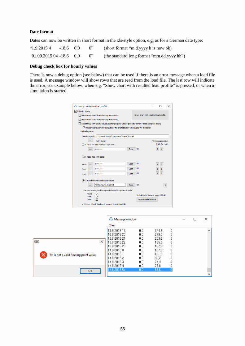
Debug check box for hourly values

There is now a debug option (see below) that can be used if there is an error message when a load file

is used. A message window will show rows that are read from the load file. The last row will indicate

the error, see example below, when e.g. “Show chart with resulted load profile” is pressed, or when a

simulation is started.

56

Miscellaneous

Fixed error “List index out of bounds” that sometimes occurred when clicking in the

configuration list.

Values for heat extraction are now shown as zeros before first month of operation.

Update 4.15 (Jan 4, 2017)

Fix: Graph for fluid temperatures was sometimes not updated when hidden.

Update 4.16 (Feb 22, 2017)

· Fix: EED showed an error message when started on systems with decimal separator "."

· Fix: Last hourly value for temperature was sometimes zero using GPU-calculation

· New "pipe.txt" file: names such as "PE DN25 PN6" changed to "PE DN25 SDR-17"

PE DN45 SDR-17 added

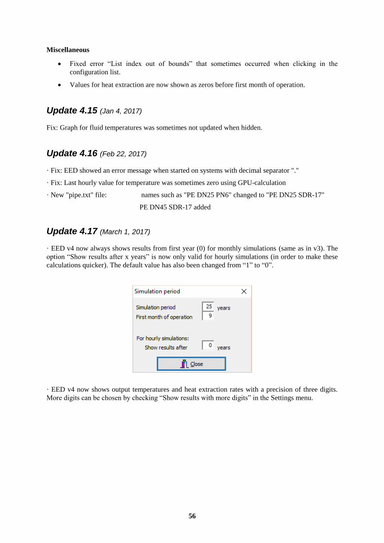
Update 4.17 (March 1, 2017)

· EED v4 now always shows results from first year (0) for monthly simulations (same as in v3). The

option “Show results after x years” is now only valid for hourly simulations (in order to make these

calculations quicker). The default value has also been changed from “1” to “0”.

· EED v4 now shows output temperatures and heat extraction rates with a precision of three digits.

More digits can be chosen by checking “Show results with more digits” in the Settings menu.