Effective Potentials and Quantum Fluid Models: AThermodynamic Approach ∗

C. Gardner†, C. Ringhofer‡D. Vasileska§

December 9, 2002

Abstract

We present a thermodynamic approach to introducing quantum corrections to the clas-sical transport picture in semiconductor device simulation. This approach leads to amodified Boltzmann equation with a quantum corrected force term and to quantumcorrected fluid, or quantum hydrodynamic models. We present the quantum inter-action of electrons with a gate oxide barrier potential and quantum hydrodynamicsimulations of a resonant tunneling diode as application examples.KEYWORDS: Quantum thermodynamics, effective potentials, quantum hydrodynam-ics

1 Introduction

A quantum mechanical description of the evolution of electron ensembles in solid state ma-terials is given by the many body Schrodinger equation for the electron ensemble. While thisequation, in combination with mean field theories and the associated Poisson equation, isable to describe ballistic transport, the inclusion of scattering mechanisms on length and timescales necessary for device simulation is still an unresolved problem. Scattering of electronswith impurities and phonons leads in general to integral operators in the resulting transport

∗This work was supported by NSF grant DECS-0218008.†Department of Mathematics, Arizona State University, Tempe, AZ 85287-1804 (gard-

ner@math.la.asu.edu).‡Department of Mathematics, Arizona State University, Tempe, AZ 85287-1804 (ringhofer@ asu.edu).§Department of Electrical Engineering, Arizona State University, Tempe, AZ 85287(vasileska@asu.edu).

1

equations which are completely non - local in space and time [2], [4], [10]. As a consequence,quantum mechanical models in device simulation usually treat quantum effects with a do-main decomposition approach, modeling ballistic transport via the mean field Schrodingerequation in ’quantum regions’, and linking them to a purely classical transport picture withcollision effects in ’classical regions’ [5], [24],[25], [26].

This paper gives an overview over a variety of alternatives to this approach, which consist ofslightly modifying classical transport models to include quantum effects, thus deriving whatcould be called quantum corrected classical transport models. The purpose of these modelsis to provide a relatively inexpensive way to include quantum effects. Therefore, the derivedmodels should in general satisfy the following criteria:

1. Their computational complexity should be comparable to their classical equivalent,i.e. drift - diffusion models, hydrodynamic models or particle based (Monte Carlo)approaches to solving the Boltzmann equation.

2. They should be corrections to this classical models in the sense that they reduce to theclassical picture in the limit ~ → 0.

3. The resulting equations should be of the same, or at least a similar, type as theirclassical counterparts.

Satisfying the first requirement allows us to perform simulations in more complex geometries,corresponding to real devices, on the same level as is done with classical models. The purposeof the second requirement is twofold. First, it allows us to easily monitor the influence ofquantum effects on solutions by comparing to the classical model equivalent. Second, itallows us to mix classical and quantum mechanical models in an engineering fashion, by,c.f. using quantum models for the electrons during free flight and semi - classical modelsfor collisions with phonons. The third requirement guarantees that the quantum correctedmodels can be linked relatively easily to the outside world by using the same type of boundaryconditions as for their classical counterparts.

We will in general consider two types of models in this paper, namely

Effective Potential Approaches:In an effective potential approach, one replaces the quantum equation by a classical equa-tion with a modified potential. Thus all the quantum effects in the system are modeledsolely through the forces acting on the electron. For this reason the same form of numericalsimulations tools can be used as for the Boltzmann transport equation, i.e. only the accel-eration terms in the free flight phase of a Monte Carlo method have to be modified. Theeffective potential approach has been applied to modeling transport in nano-scale MOSFETswith gate length of 25 nm that are of both industrial and scientific interest. We find that

2

the inclusion of the barrier potential into a classical Monte Carlo particle-based simulationscheme, details of which are given in Section 8, gives rise to on-state current reduction ofabout 20 % due to the displacement of the charge from the interface and the introductionof the inversion layer capacitance that degrades the oxide capacitance and, therefore, theMOSFET transconductance. The approach proposed here is compared to a similar approachby Ferry and coworkers [1], in which the effective potential is calculated as a convolution ofa Gaussian function and the Hartree potential obtained from solving the two-dimensional orthree-dimensional Poisson equation.

Quantum Fluid Models:These models are derived in general from moment closures of quantum kinetic transportequations, like the Wigner equation. They involve roughly the same level of computationalcomplexity as the classical drift - diffusion systems and hydrodynamic equations. On thislevel of modeling collisions appear only through relaxation times and diffusion coefficients,which are taken from classical theory. Quantum fluid models have been used successfully inthe simulation of hetero -structure devices whose function is based on quantum tunnelingphenomena. There, they are able to predict negative differential resistance as well as resonanttunneling phenomena [11], [13].

This paper is organized as follows. Effective potentials as well as fluid models are derived froma quantum mechanical description, either in form of the Schrodinger equation or a quantumkinetic transport equation for the Wigner function. In Section 2 we present these equationsin a setting appropriate for our purposes and in Section 3 we give the general setting for theeffective potential and moment closure approach. The approach mainly considered in thispaper is a thermodynamic one, and relies on an appropriate quantum representation of thethermodynamic equilibrium state. We discuss this representation and its approximations inSections 4 and 5. Sections 6 and 7 contain the derivation of effective potentials and momentclosures based on this thermodynamic approach. Section 8 gives a glimpse on simulationresults for the for interaction of electrons with the Si − SiO2 interface in a short channelMOSFET, using effective potentials and a resonant tunneling diode using a quantum fluidmodel.

2 Quantum Kinetic Equations

In this section we give brief overview over the kinetic equations and their relation to thequantum mechanical transport picture. The purpose of this section is mainly to providean appropriate framework for the following derivation of macroscopic apprroximations andeffective potentials. We start with the Schroedinger equation for a mixed state. The transient

3

Schrodinger equation for the wave function ψλ is given by

i~∂tψλ = Hψλ := − ~2

2m∗∆xψλ + e(V C + V B)(x, t)ψλ, (1)

where ψλ(x, t) is the wave function corresponding to the energy level λ, ~ denotes Planck’sconstant andm∗ is the effective mass of the electron. The effective single electron Schroedingerequation (1) is already derived from a mean field approximation for the many body Schrodingerequation. Therefore, if the forces between the electrons are Coulomb forces, the Hartree po-tential V C(x, t) in (1) is given by the Poisson equation

∇x · ε∇xVC = e(n−D) (2)

where ε and e denote the dielectric tensor and the electron charge respectively. D(x) denotesthe usual doping concentration and n(x, t) is the number density of electrons given by

n(x, t) =∑

λ

F (λ)|ψλ(x, t)|2 . (3)

The summation in (3) ranges over the whole spectrum of the Hamiltonian H in (1) and F (λ)denotes a given statistical distribution function. The potential V B in (1) denotes the bandgapof the given material. If only one type of material is considered V B can be taken to be equalto zero. However, in device simulation it is usually necessary to consider geometries madeup of several materials and V B is will in general a discontinuous function taking on differentconstant values in the semiconductor and the gate oxide or in the different materials makingup a hetero - junction device. The Schrodinger Poisson system (1)-(2) is the most accuratedescription of purely ballistic transport. It does, however, bear some severe disadvantagesfor the actual use in device simulation. These are:

1. It does not include any scattering mechanisms important to the actual function ofdevices.

2. It still has to be linked to the outside world via boundary conditions which are nottrivial in the case of contacts and interfaces.

3. Its steady state is given by the solution of an eigenvalue problem for the energies λand cannot be computed by simply setting formally ∂tψλ = 0 in (1).

The above problems are usually overcome in practice in the following way:The Schrodinger equation (1) is linked to the outside world by setting potentials constantand assuming a plain wave solution outside the domain of computation. This plain wavesolution is then linked via continuity conditions to the solution inside the computationaldomain. Since now the steady state eigenvalue problem Hψλ = λψλ has a continuousspectrum, solving the eigenvalue problem is actually replaced by solving a boundary value

4

problem for the Hamiltonian for a select set of eigenvalues λ. In one dimension this approachtakes the following form:If the simulation domain (in one dimension) consists of the interval [−L,L], then we assumea plain wave solution of the form

ψλ(x) = eiξx +Re−iξx for x < −L

This corresponds to injecting an electron with positive momentum ~ξ from the left into thedomain. This gives the relation λ = λ(ξ) = ~2ξ2

2m∗+ eV − between the eigenvalue λ and the

wave number ξ, where V − denotes the constant value of the potential to the left of x = −L.The corresponding plane wave solution to the right of the interval [−L,L] is given by

ψλ(x) = Teiη(ξ)x for x > L, η(ξ) =

√2m∗

~2(λ(ξ)− eV +) =

√ξ2 +

2em∗

~2(V − − V +) ,

where V + denotes the constant value of the potential for x > L. It remains to compute thereflection and transmission coefficients R and T . They can be eliminated by matching thewave function and its derivative to the outer solutions, giving the boundary conditions

∂xψλ + iξψλ|x=−L = 2iξe−iξL, ∂xψλ − iη(ξ)ψλ|x=L = 0. (4)

Thus, for a given set of wave numbers ξ, a boundary value problem of the form Hψλ(ξ) =λ(ξ)ψλ(ξ), together with the boundary conditions (4) has to be solved. A symmetric pro-cedure has to be carried out, injecting electrons from the x > L and the solution is thenpieced together, using the statistic F (λ) in (3). Starting from the so constructed equilibriumstate a system of transient Schrodinger equations (1) can then be solved using the boundaryconditions (4). This whole procedure becomes of course significantly more complicated inmore than one spatial dimension and several approximations have to be used. We refer thereader to [26],[24],[25] for an overview.

The basic concept outlined above does, however, not yet address the issue of collisions.These are incorporated by linking the ballistic quantum transport picture to a classicaltranport equation (either the Boltzmann equation on a kinetic level or hydrodynamics on amacroscopic level) and by assuming that quantum effects and collisions are not relevant inthe same subdomains. It should be mentioned that this linkage still poses some problems inmaintaining momentum conservation [5].

Quantum corrections to the classical transport picture present an alternative to the approachoutlined above. They start from formally transforming the Schrodinger - Poisson system (1)-(2) into a transport equation which is the analog of the collisionless Boltzmann equation.The tool for this is the Wigner transform [31], given by

f(x, p, t) = (2π)−3

∫R3

ρ(x+~2η, x− ~

2η) exp(iη ·p) dη, ρ(x, y, t) :=

∑λ

F (λ)ψλ(x)∗ψλ(y) ,

(5)

5

where ρ(x, y, t) denotes the density matrix of the mixed state. f(x, p, t), the Wigner function,is a quasi - probability, and the equivalent of the kinetic density in the Boltzmann equation,i.e. f is a function of position x and momentum p. Direct calculus yields that positivedefinite density matrices ρ correspond to real Wigner functions f and that

n(x, t) =

∫R3

f(x, p, t) dp = ρ(x, x, t) =∑

λ

F (λ)|ψλ(x, t)|2

holds. Direct calculus again yields that, if the wave functions ψλ satisfy the Schrodingerequation (1), the Wigner function f satisfies the Wigner equation

∂tf +1

m∗∇x · (pf)− eθ[V ]f = 0 , V := V C + V B, (6)

with the operator θ[V ] given by

θ[V ] =i

~[V (x+

~2i∇p)− V (x− ~

2i∇p)] .

The operator θ[V ] has to be understood in the sense of pseudo - differential operators. Sothe action of θ[V ] is given by

θ[V ]f(x, p, t) = (2π)−3

∫R3

∫R3

i

~[V (x+

~2η)− V (x− ~

2η)]f(x, q, t) exp[iη · (p− q)] dqdη .

At least on a purely formal level, the pseudo differential operator θ[V ] tends to the classicalacceleration term ∇xV · ∇p in the classical limit for ~ → 0, and therefore, on a formal levelagain, the Wigner equation (6) tends to the Vlasov equation

∂tf +1

m∗∇x · (pf)− e∇p · (∇xV f) = 0 .

It is this similarity which is exploited in the general approach to quantum corrections toclassical kinetic and fluid dynamic modeling. So the starting point of quantum correctionsto the classical transport picture will be the Wigner - Boltzmann - Poisson system

(a) ∂tf +1

m∗∇x · (pf)− eθ[V ]f = Q(f) (7)

(b) ∇ · ε∇V = e(n−D), n(x, t) =

∫R3

fx, p, t) dp ,

where Q(f) denotes the collision operator. In the case of fluid approximations only theknowledge of the moments of the collision operator Q, i.e. the relaxation times, are requiredand we will assume those to be given by the classical theory.

6

3 Moment Closures and Effective Potentials

In this section we will introduce the concept of effective potentials and give the formalderivation of the moment system for the Wigner - Boltzmann - Poisson system (7). Westart with the most famous effective potential approximation, the Bohm - potential, whichis exact for a single pure state.

3.1 Bohm Potentials

Writing the complex wave function ψλ in (1) in terms of its amplitude and phase, i.e.

ψλ = aλ exp(iφλ)

we obtain the Schrodinger equations for amplitude and phase of the form

∂t ln(aλ) +~

2m∗[∆φλ + 2∇ ln(aλ) · ∇φλ] = 0

~∂tφλ +~2

2m∗[|∇φλ|2 −

∆aλ

aλ

] + eV = 0 .

Setting nλ = a2λ and ∇φλ = m∗

~ uλ, we obtain formally a zero temperature Euler equationwith a corrected potential term for the amplitude and phase of each wave function of themixed state.

(a) ∂tnλ +∇ · (nλuλ) = 0 (8)

(b) ∂t(m∗nλuλ) +∇ · (m∗nλuλuTλ ) + nλ∇[eV − ~2

2m∗

∆√nλ√nλ

] = 0, V = V C + V B .

In the derivation of (8)(b) we have made use of the fact that each individual uλ is a gradient

field. The corrected potential V Q = V C + V B − ~2

2em∗

∆√

nλ√nλ

is called the Bohm potential [8].

Alternatively, the quantum correction in the potential can be included as a pressure termby writing the momentum equation (8)(b) as

∂t(m∗nλuλ) +∇ · [nλ(m∗uλuTλ − ~2

4m∗∇2 ln(nλ))] + enλ∇V = 0, V = V C + V B . (9)

So, to reproduce the Schrodinger equation (1) one solves the system (8) for each energy λ andcomputes the total densities according to the statistics used in (3). Each of the equations(9) represents the movement of a single electron, and is therefore given at zero temperature.The temperature of the ensemble has to be computed from the variance among the differentuλ. Although (8) has the appearance of a fluid equation it is completely equivalent to theSchrodinger equation, and therefore is not really a macroscopic or fluid approximation. Fluidapproximations at finite temperature are obtained from (8) in the following, more or less ad

7

hoc, way [15], [16], [17] [18]. Starting from a single nonlinear Schrodinger equation, wherethe potential is written as V = V C +V B +V NLS(|ψ|2) the same procedure as outlined abovecan be repeated, leading to

∂t(m∗nu) +∇ · [n(m∗uuT − ~2

4m∗∇2 ln(n))] + en∇(V C + V B + V NLS(n)) = 0 .

The nonlinear potential term ∇V NLS can be absorbed into a stress tensor by introducingthe function P (n) as P0(n) = −e

∫n d

dnV NLS(n) dn, giving

∂t(m∗nu) +∇ · [n(m∗uuT − ~2

4m∗∇2 ln(n))− P0(n)I] + en∇(V C + V B) = 0 . (10)

This is the approach taken in [15], [16] and [17] and basically assumes that, somewhat in thespirit of density functional theory, the properties of the electron ensemble can be replacedby an effective single electron picture, using the right potential. So there is a one to onerelation between each scalar form the stress tensor P = P0 I and the nonlinear potential. Soc.f. a constant temperature P0 = −nKT0 would correspond to a logarithmic nonlinearity inthe Schrodinger equation eV NLS = KT0 ln(n).

3.2 Thermodynamic Approximations

In this paper we take a different approach, namely to derive effective potential as well as fluidapproximations via a thermodynamic argument. We start from the Wigner - Boltzmann -Poisson equation (7) and transform it first to center of mass coordinates. We define themean velocity u(x, t) of the ensemble by∫

R3

pf(x, p, t) dp = m∗un(x, t), n(x, t) =

∫R3

f(x, p, t) dp ,

and choose m∗u as the origin of the coordinate system in momentum space, i.e. we chooseLagrangian instead of Eulerian coordinates. Defining fL(x, p, t) = f(x, p + m∗u(x, t), t) weobtain the Wigner - Boltzmann equation

∂tfL+

1

m∗∇x ·[(p+m∗u)f

L]−∇p ·{fL[m∗∂tu+((p+m∗u)·∇x)u]}−θ[V ]fL = QL(fL) , (11)

where we also shift the collision operator Q, i.e. QL(fL)(x, p, t) = Q(f)(x, p+m∗u, t) holds.Note that, by definition, the first order moment of fL vanishes identically, i.e.

∫pfL dp = 0

always holds. The basic idea is to choose approximations which are exact if the momentumcentered density fL is given by the thermal equilibrium density. In the classical case thiswould correspond to

fL(x, p, t) = exp[−β|p|2

2m∗− eβV (x, t)] (12)

8

with β = (KT )−1 the equilibrium temperature. In quantum mechanics thermal equilibriumis characterized by the density matrix ρ corresponding to the Wigner function fL being givenby F (βH) with H the Hamiltonian H = − ~2

2m∗∆ + eV and F the statistical distribution

function used, i.e. the Boltzmann or the Fermi - Dirac statistic. Using the definition (5) ofthe Wigner function this means

(a) f eq(x, p) = (2π)−3

∫R3

ρeq(x+~2η, x− ~

2η) exp(iη · p) dη, (13)

(b) ρeq(x, y) :=∑

λ

F (βλ)ψeqλ (x)∗ψeq

λ (y) ,

(c) (− ~2

2m∗∆ + V )ψeq

λ = λψeqλ .

Of course f eq as well as the eigenfunctions ψeqλ will depend on the the time t throught he

potential V , since we only assume a local in time equilibrium for a given time dependentpotential. The Function F (z) is either given by F (z) = eφ−z in the case of Boltzmannstatistics or by F (z) = (1 + cez−φ)−1 in the case of Fermi - Dirac statistics.

Effective Potentials:The effective potential approximation is now given by replacing the pseudo differential op-erator θ[V ] in (11) by a classical counterpart

θ[V ]f → ∇p · [f∇xVQ(x, p, t)] (14)

in such a way that (14) is exact for fL = f eq given by (13). Because of the equilibriumproperty this implies that

f eq(x, p) = exp[−β|p|2

2m∗− βeV Q(x, p)]

holds.

Quantum Hydrodynamics:To consider fluid approximations to the momentum centered Wigner - Boltzmann equation(11) we take, following [11],[12], the first three moments of (11), corresponding to massmomentum and energy, and obtain

(a) ∂tn+∇x · (nu) = 0 (15)

(b) ∂t(nm∗u) +∇x · (m∗nuuT )−∇x · P + n∇xV = 〈pQ0〉

(c) ∂t(3nKT ) +∇x · (3nKTu+ 2q)− 2Tr(P∇Txu) = 〈|p|

2

m∗Q0〉 ,

where we define temperature T , stress tensor P and heat flux q in the usual way by

(a) P = − 1

m∗

∫R3

ppTfL dp, (b) 3nKT = −Tr(P ) =1

m∗

∫R3

|p|2fL dp, (16)

9

(c) q =1

2m2∗

∫R3

p|p|2fL dp .

Here K denotes the Boltzmann constant. The moment system (15) has to be closed byexpressing the P and q in terms of the primary variables n, u, T (charge, velocity, tempera-ture). Models for the moments of the collision operator Q have to be assumed and a varietyis readily available in the literature [3], [28], the simplest being the relaxation time models

〈pQ0〉 = −nm∗

τpu, 〈|p|

2

m∗Q0〉 =

3nK(T0 − T )

τw

with relaxation times τp and τw. In the context of thermodynamic approximations this isdone by setting again fL = f eq and deriving the appropriate relations from (13). Notethat the moment system (15) is identical to the classical moment system, leading to thecompressible Euler equations, since the first three moments of the pseudo differential operatorθ[V ]f coincide with the moments of its classical counterpart ∇p · (f∇xV ). The quantumcorrections therefore will appear only in the closure relations. In the classical case, with fL

given by (12), one obtainsP = −nKT Id, q = 0,

where Id denotes the identity matrix, and the quantum corrections will enter only throughthe difference between (12) and (13). For the purpose of actual numerical discretization itis beneficial to write (15)(c) in conservative form, expressing the balance of the total energyinstead of the thermal energy 3nKT . Multiplying (15)(a) with −m∗|u|2 and (15)(b) with2uT and adding to (15)(c) gives

∂t(m∗n|u|2 + 3nT ) +∇x · [m∗n|u|2u+ 3nTu+ 2q]− 2∇x · (Pu) + 2nuT∇xV =

〈(2uTp+|p|2

m∗ )Q0〉 =1

m∗〈|p+m∗u|2Q0〉

4 Thermodynamic Equilibrium

This section is concerned with the derivation of the equilibrium density f eq in (13). Although(13) completely defines the thermodynamic equilibrium in terms of the Hamiltonian, andtherefore in terms of the potential V , we will need an explicit expression for f eq in order toobtain a formula for the effective quantum potential V Q in (14) and the closure momentsP and q in (15). Of course, it is not possible to find an exact expression for f eq, and wewill need some kind of approximate formula. These approximations will be the subject ofthe next two sections. In this section we will give a form of the equilibrium density whichis appropriate for the derivation of such approximations, i.e. some alternative way to solvethe eigenvalue problem for the wave functions ψeq

λ . For the case of Boltzmann statisticsthis alternative way is given by the Bloch equation. The Bloch equation is a formal way to

10

replace the computation of the exponential of a density matrix by the solution of a parabolicdifferential equation. We define the equilibrium density matrix ρeq(x, y, β) as the exponentialof the Hamiltonian by

ρeq(x, y, β) =∑

λ

exp[β(φ− λ)]ψeqλ (x)∗ψeq

λ (y) ,

where the ψeqλ are the normalized eigenfunctions of the Hamiltonian H = − ~2

2m∗∆ + eV .

Evaluating ρeq at β = 0 gives, because of the mutual orthogonality of the eigenfunctions,ρeq(x, y, 0) = δ(x− y). Differentiating ρeq with respect to the inverse temperature β gives

∂βρeq(x, y, β) =

∑λ

exp[β(φ− λ)](φ− λ)ψeqλ (x)∗ψeq

λ (y) .

Applying the Hamiltonian H to the density matrix ρeq gives

Hρeq =∑

λ

exp[β(φ− λ)]λψeqλ (x)∗ψeq

λ (y) = ρeqH ,

Because of the eigenfunction property of the ψeqλ and the fact that ρeq commutes with the

Hamiltonian. Thus the equilibrium density matrix ρeq satisfies the initial value problem

∂βρeq(x, y, β) = −1

2(Hρeq + ρeqH) + φρeq, ρeq(x, y, 0) = δ(x− y) ,

where Hρeq denotes the usual matrix product, or, evaluating the Hamiltonian,

∂βρeq(x, y, β) =

~2

4m∗(∆x+∆y)ρ

eq− e2[V (x)+V (y)]ρeq+φρeq, ρeq(x, y, 0) = δ(x−y) . (17)

(17) is called the Bloch equation for the equilibrium density matrix.

Remark: We have symmetrized the Bloch equation (17) in order to make it obvious thatthe equilibrium density matrix ρeq will always be real and self adjoint.

So we have replaced the solution of the eigenvalue problem for the Hamiltonian H by solvingthe parabolic initial value problem (17) in twice as many spatial dimensions. This doesnot make the problem computationally easier, but more amenable to asymptotic analysis.Physically the Bloch equation has the interpretation that we start from a totally uncorrelatedstate at infinite temperature (β = 0) and smooth out to a state at finite temperature (β > 0).Computing the Wigner transform f eq of ρeq, according to (13), gives the initial value problem

∂βfeq(x, p, β) =

~2

8m∗∆xf

eq − |p|2

2m∗f eq − eω[V ]f eq + φf eq, f eq(x, p, 0) = ~−3 , (18)

with the pseudo differential operator ω given by

ω[V ] =1

2[V (x+

~2i∇p) + V (x− ~

2i∇p)]

or

ω[V ]f(x, p) =1

2(2π)−3

∫R3

∫R3

[V (x+~2η) + V (x− ~

2η)]f(x, q) exp[iη · (p− q)] dqdη

11

5 Approximations to Thermal Equilibrium

We now turn to the derivation of approximate formulas for the thermodynamic equilibriumstate given by the solution of the Bloch equation (18). The advantage of the Bloch equationis that asymptotic formulas for the equilibrium state can be found more easily form (18) thanfrom the solution of the eigenvalue problem. We will use two different types of asymptoticformulas. The first is derived from the semiclassical regime (i.e. ~ → 0). This leadsessentially again to the Bohm potential. The disadvantage of the semiclassical approximationis twofold: First it assumes that the Planck constant is small compared to the involvedspatial and time scales. This is in general not the case for small quantum devices such as c.f.resonant tunneling diodes. Second, the resulting approximations involve higher derivativesof the potential, i.e. they hold only for sufficiently smooth potentials and are not valid inthe vicinity of dicontinuous potential barriers. We therefore present another approximation,which assumes neither smooth potentials nor the semiclassical regime but instead is basedon the assumption that the unbounded operators in the Bloch equation will dominate thebounded operators.

5.1 Semiclassical Approximations

Assuming a sufficiently smooth potential V the pseudo differential operator ω in (18) can beexpanded in powers of ~, giving

ω[V ]f = V f − ~2

8Tr[(∇2

xV )(∇2pf)] +O(~4) .

For reasons of notational convenience we introduce the parameter α = ~2

8m∗and write the

expanded equation (18) as

∂βfeq(x, p, β) = α∆xf

eq− |p|2

2m∗f eq−eV f+eαm∗Tr[(∇2

xV )(∇2pf

eq)]+φf eq, f eq(x, p, 0) = ~−3

We expand the equilibrium Wigner function f eq as f eq = ~−3(f0 + αf1 + ...) and obtain forthe zero and first order term

(a) ∂βf0(x, p, β) = − |p|2

2m∗f0 − eV f0 + φf0, f0(x, p, 0) = 1 (19)

(b) ∂βf1(x, p, β) = ∆xf0 −|p|2

2m∗f1 − eV f1 + em∗Tr[(∇2

xV )(∇2pf0)] + φf1, f1(x, p, 0) = 0

The zero order term can be computed immediately from (19)(a) as

f0(x, p, β) = exp[−β|p|2

2m∗+ β(φ− eV )] . (20)

12

In order to compute f1 form (19)(b) via variation of constants we set f1 = gf0 and obtain

∂βg(x, p, β) =∆xf0

f0

+em∗

f0

∇2xV : ∇2

pf0, g(x, p, 0) = 0

as the initial value problem for g. Using the formula (20) for f0 we compute the terms onthe right hand side as

∂βg(x, p, β) = −βe∆xV + β2e2|∇xV |2 + em∗Tr[(∇2xV )(− β

m∗I +

β2

m2∗ppT )], g(x, p, 0) = 0

or

∂βg(x, p, β) = −2βe∆xV + β2e2|∇xV |2 +eβ2

m∗Tr[(∇2

xV )ppT ], g(x, p, 0) = 0

and after integration

g(x, p, β) = −β2e∆xV +β3e2

3|∇xV |2 +

eβ3

3m∗Tr[(∇2

xV )ppT ] .

This gives the approximate formula for the thermal equilibrium Wigner function f eq as

~3f eq(x, p, β) = (21)

exp[−β|p|2

2m∗+β(φ− eV )]{1− β2e~2

8m∗∆xV +

β3e2~2

24m∗|∇xV |2 +

eβ3~2

24m2∗Tr[(∇2

xV )ppT ]}+O(~4) .

Clearly, (21) is an order ~2 correction to the classical thermal equilibrium given by theMaxwellian. The total number of electrons in the equilibrium state is given by the QuasiFermi potential φ.

5.2 Born Approximations

As mentioned, the disadvantage of the approximate expression (21) for the thermal equilib-rium Wigner function is that it involves higher order derivatives of the potential V which,in the case of dicontinuous barrier potentials, will only exist in a distributional sense. Wetherefore give a different type of asymptotic solution. The basic assumption is that the un-bounded operator (the Laplacian) in (18) dominates the potential term. So we formally setV = εVε and expand the solution of (18) in powers of the parameter ε. It should be pointedout that ε is a purely formal parameter and that the procedure below corresponds to theBorn approximation of e−βH [13], [14]. So we expand the solution of

∂βfeq(x, p, β) = α∆xf

eq − |p|2

2m∗f eq − eεω[Vε]f

eq + φf eq, f eq(x, p, 0) = ~−3 (22)

13

in powers of the artificial parameter ε. α in (22) denotes again the quantity ~2

8m∗, but now is

not assumed to be small. Similarly to the previous case, we again set f eq = ~−3(f0 + εf1),and obtain

(a) ∂βf0(x, p, β) = α∆xf0 −|p|2

2m∗f0 + φf0, f0(x, p, 0) = 1 (23)

(b) ∂βf1(x, p, β) = α∆xf1 −|p|2

2m∗f1 − eω[Vε]f0 + φf1, f1(x, p, 0) = 0

as the equations determining f0 and f1. Again, (23)(a) can be solved immediately, giving

f0 = exp[βφ− β|p|2

2m∗] . (24)

Solving (23)(b) turns out to be a bit more technically involved since we have to use theGreens function for the heat operator. This is done best by Fourier transforming (23)(b) inspace, and writing f1 as a pseudo differnetial operator acting (in the spatial direction) onthe potential Vε. We define

g(ξ, p, β) = (2π)−3

∫R3

f1(x, p, β) exp(−iξ · x) dx, V (ξ) = (2π)−3

∫R3

Vε(x) exp(−iξ · x) dx ,

and obtain

∂βg(ξ, p, β) = −α|ξ|2g − |p|2

2m∗g − eR(ξ, p, β)V + φg, g(ξ, p, 0) = 0 (25)

as the initial value problem defining the Fourier transform g(ξ, p, β), where the termR(ξ, p, β)Vis the Fourier transform in the spatial direction of ω[Vε]f0.

R(ξ, p, β)V (ξ) = (2π)−3

∫R3

ω[Vε]f0(x, p, β)e−iξ·x dx

holds. A direct calculation, using the definition of the pseudo differential operator ω[Vε]yields

R(ξ, p, β) =1

2exp[βφ](2π)−3/2

∑σ=±1

∫R3

exp[i

√β

m∗η · (p+ σ

~2ξ)− |η|2

2] dη

R(ξ, p, β) =1

2exp[βφ]

∑σ=±1

exp[− β

2m∗|p+ σ

~2ξ|2] . (26)

Inserting (26) in (25) and solving the ordinary differential equation gives

g(ξ, p, β) = −eβV (ξ) exp[−αβ|ξ|2 − β|p|2

2m∗+ βφ]

∫ 1

0

cosh[γβ~2m∗

p · ξ] dγ .

Reversing the Fourier transforms, we obtain the first order term f1 as

f1(x, p, β) =

14

−eβ(2π)−3

∫R3

∫R3

∫ 1

0

Vε(y) exp[−αβ|ξ|2 − β|p|2

2m∗+ βφ] cosh[

γβ~2m∗

p · ξ] exp[iξ · (x− y)] dγdydξ

which we write, formally, as a pseudo differential operator S in the spatial direction, actingon the potential Vε:

f1(x, p, β) = − exp[βφ]S(−i∇x, p, β)Vε (27)

with the symbol S given by

S(ξ, p, β) =eβ

2

∑σ=±1

∫ 1

0

exp[αβ(γ2 − 1)|ξ|2 − β

2m∗|p+

σγ~2ξ|2] dγ, α =

~2

8m∗(28)

So, combining (24) and (27) and setting V = εVε again, the Born approximation approxi-mation formula to the thermal equilibrium state is given by

~3f eq(x, p, β) ≈ exp(βφ)[exp(−β|p|2

2m∗)− S(−i∇x, p, β)V ] (29)

with the symbol of the operator S given by (28). Note that S is actually a smoothingoperator. It can be shown that for large ξ the symbol S behaves like O( 1

|ξ|2 ). Therefore theterm SV will actually have two more classical derivatives than the original potential V .

6 Effective Potentials and Particle Discretizations

The goal of the effective potential approach is to incorporate quantum corrections into par-ticle based simulators by replacing the classical forces moving the electron during the freeflight by modified quantum forces. So, in the semiclassical Boltzmann equation

∂tf +∇x(1

m∗pf)−∇p(ef∇xV ) = Q(f)

the field term −e∇xV (x, t) is replaced by a modified quantum field term −e∇xVQ(x, p, t).

Given an existing particle based simulator, this is, at least in theory, easily achieved bycomputing the trajectories of electrons via

d

dtx =

1

m∗p,

d

dtp = −e∇xV

Q(x, p),

where the time dependence of the potential is frozen during the free flight phase. Thisapproach is computationally much easier than trying to solve the Wigner equation (6) directlyby a particle based method (see [6], [7] [29] and reference therein). There, however, are twoimportant points which should be mentioned here

1. Representing the density function as a simultaneous δ− function in space and momen-tum violates the Heisenberg principle.

15

2. Just modifying the forces will invariably result in a strictly positive phase space densityf while the Wigner function can become locally nonpositive.

So, this approach is not an exact representation of quantum mechanics. It can, however,represent certain quantum effects, such as the nonlocal interaction of electrons with barrierpotentials and even tunneling. On the other hand, it allows for the immediate incorpora-tion of all the relevant semiclassical scattering mechanisms usually included in Monte Carlosimulations. The use of more quantum mechanically correct collision operators is still verymuch an open research topic [2], [4], [10]. Using the Bohm potential from Section 3.1 theeffective quantum potential V Q is given by

eV Q = eV − ~2

2m∗

∆√n√n

. (30)

The same quantum corrected potential can be obtained from the semiclassical approximationto the thermal equilibrium state in Section 5.1. The evaluation of (30) poses a significantchallenge in the context of particle based discretizations. The number density n is givenby a superposition of δ− functions in physical space of which the third derivative has to becomputed to evaluate the force. This can be either done by computing n on a mesh usingthe usual cloud in cell approach and then using a difference discretization, or by computingthe third derivatives directly in a meshless approach [32] , [33]. The first approach requiresa considerable amount of smoothing.

Alternatively, one can use the Born approximation to the thermodynamic equilibrium statein Section 5.2 by requiring that replacing term θ[V ]f by ∇p(f∇xV

Q) in the Wigner equation(6) is exact in thermal equilibrium, i.e. by writing

~3f eq = exp[βφ− β|p|2

2m∗− βeV Q(x, p, β)] ,

with f eq given by (29). This gives the effective quantum potential V Q as

V Q(x, p, β) =1

βeexp(

β|p|2

2m∗)S(−i∇x, p, β)V (x) , (31)

with the symbol of the operator S given, according to (28), by

S(ξ, p, β) =eβ

2

∑σ=±1

∫ 1

0

exp[αβ(γ2 − 1)|ξ|2 − β

2m∗|p+

σγ~2ξ|2] dγ, α =

~2

8m∗

The symbol S can be simplified to give

S(ξ, p, β) = eβ exp(−β|p|2

2m∗− αβ|ξ|2)

∫ 1

0

cosh(γβ~p · ξ

2m∗) . (32)

16

Combining (31) and (32) gives

V Q(x, p, β) = exp(αβ|∇x|2)2m∗

iβ~p · ∇x

sinh(iβ~p · ∇x

2m∗)V (x)

or

(a) V Q(x, p, β) = (2π)−3

∫R3

∫R3

Γ(ξ, p, β)V (y) exp[iξ · (x− y)] dydξ (33)

(b) Γ(ξ, p, β) = exp(−β~2|ξ|2

8m∗)

2m∗

β~p · ξsinh(

β~p · ξ2m∗

)

The quantum potential (33) is a more sophisticated version of the smoothed potential, basedon wave packet analysis, presented in [27]. We note that, in general, the evaluation ofsmoothed potentials in the context of particle based methods is a quite expensive enterprise,since the smoothed potentials are computed as convolutions of the Coulomb and barrierpotential V C , V B with a Gaussian type kernel, and have to be evaluated for every electron.This is therefore done by tabulating the potential and subsequent interpolation. Since thesmoothed potential in (33) is given in terms of Fourier transforms, the use of fast Fouriertransform algorithms is essential for this task. Alternatively, in certain device structures,one can use the effective potential V Q only for the barrier part and take the action of theCoulomb potential to be classical, since in many applications the quantum action of theCoulomb potential is negligible [30].

We conclude this section by giving the smoothed effective quantum potential (33) for thecase of a single potential step. Multiple steps and barriers can be easily combined from thesingle step case. We assume the potential step to occur along a plane in three dimensionalspace through a point r with unit normal vector n. So the potential gradient is given by∇xV = V0δ((x − r) · n)n with V0 the height of the step. Inserting this potential gradientinto (33), we obtain

∇xVQ(x+ r, p, β) = n(2π)−3V0

∫R3

∫R3

Γ(ξ, p, β)δ(y · n) exp[iξ · (x− y)] dydξ

∇xVQ(x+ r, p, β) =

n(2π)−3V0

∫R3

∫R3

Γ(ξ0n + ξ⊥, p, β)δ(y0) exp[iξ0(n · x− y0) + iξ⊥ · (x− y⊥)] dy0y⊥dξ0ξ⊥

where we have decomposed the variables ξ and y into their components parallel (ξ0n, y0n)and orthogonal (ξ⊥, y⊥) to n. The integral with respect to y⊥ yields a δ− function in ξ⊥,giving

∇xVQ(x+ r, p, β) = n(2π)−1V0

∫Γ(ξ0n, p, β) exp[iξ0n · x] dξ0 (34)

with, according to (33)(b), Γ(ξ0n, p, β) given by

Γ(ξ0n, p, β) = exp(−β~2ξ20

8m∗)

2m∗

β~p0ξ0sinh(

β~p0ξ02m∗

), p0 := p · n .

17

Inserting this into (34) gives

∇xVQ(x+ r, p, β) = n(2π)−1V0

∫ 1

0

∫R

exp(−β~2ξ20

8m∗) cosh(

γβ~p0ξ02m∗

) exp[iξ0n · x] dξ0dγ =

n(2π)−1V01

2

∑σ=±1

∫ 1

0

∫R

exp[−β~2ξ20

8m∗+ iξ0(n · x− iσγβ~p0

2m∗)] dξ0dγ

and finally,

∇xVQ(x, p, β) = n(2π)−1/2V0

√m∗

β~2

∑σ=±1

∫ 1

0

exp[−2m∗

β~2(n · (x− r)− iσγβ~p0

2m∗)2] dγ . (35)

7 Quantum Hydrodynamics

Given an approximate solution to the thermal equilibrium Wigner function f eq one can nowproceed to find equations of state for the stress tensor P and the heat flux q in (15) in Section3 by computing P and q from the equilibrium density f eq. This is done by using a functionalexpansion of the equilibrium Wigner function. First, we note that the solution f eq of theBloch equation (18) will always be an even function of the momentum p. Therefore the oddmoments of f eq, including the heat flux, vanish. As in the classical case, a nonzero heat fluxhas to be derived by using the collision operator in a Chapman - Enskog type procedure.The stress tensor P is derived by a functional expansion of the equilibrium Wigner functionf eq in Section 5, using either the semiclassical or the Born approximation.

7.1 The semiclassical closure

In the semiclassical approximation of the equilibrium density is given in terms of an expansionof the parameter α = ~2

8m∗. Consequently, we express the stress tensor P as a function of the

density n of the asymptotic form

P = P0(n, β) + αP1(n, β) +O(α2) . (36)

Since the charge density n is itself expanded in powers of α, i.e. computing the zero ordermoment of (21) with respect to p we obtain n = n0 + αn1 +O(α2), we have, up to terms oforder α2

P = P0(n0, β) + α∂nP0(n0, β) + αP1(n0, β) +O(α2) .

From (21) we have~3f eq = (37)

18

exp[−β|p|2

2m∗+ β(φ− eV )]{1− β2eα∆xV +

β3e2α

3|∇xV |2 +

eβ3α

3m∗Tr[(∇2

xV )ppT ]}+O(α2) .

Computing the integral of (37) with respect to momentum one obtains

(a) n = n0[1 +αβ3e2

3|∇xV |2 −

2αeβ2

3∆xV +O(α2)], (38)

(b) n0 := ~−3

∫R3

exp[−β|p|2

2m∗+ β(φ− eV )] dp

and therefore the first order term n1 is given by

n1 = n0[β3e2

3|∇xV |2 −

2eβ2

3∆xV ] .

Computing the integral in (38), we see that n0 equals a constant times exp(−eβV ). Thereforewe can replace derivatives of eβV in the expression for n1 by derivatives of − lnn0 and obtain

n1 = n0[β

3|∇x lnn0|2 +

2β

3∆x lnn0] .

Computing the stress tensor according to (16) from (37) we obtain

Pjk = − 1

m∗

∫R3

pjpkfeq dp = −n0[δjk(

1

β− 2

3αβe∆xV +

αβ2e2

3|∇xV |2) +

2αeβ

3∂jkV ]

up to terms of order α2. this gives for P0

P0(n0, β) = −n0

βI, ∂nP0(n0, β) = − 1

βI ,

where again I denotes the identity matrix. Inserting the above into (36) yields

−n0

βI − αn0[

1

3|∇x lnn0|2 +

2

3∆x lnn0]I + αP1(n0, β) =

−n0[I(1

β+

2

3α∆x lnn0 +

α

3|∇x lnn0|2)−

2α

3∇2 lnn0] ,

which yields for the functional form of P1

P1(n, β) =2n

3∇2 lnn ,

or, altogether

P (n, β) = −nKT I +n~2

12m∗∇2 lnn, KT :=

1

β(39)

19

7.2 Smoothed Potential QHD based on the Born Approximation

The same procedure, namely using the asymptotic expression for the thermal equilibriumWigner function f eq to derive a functional expansion of the stress tensor P can be appliedto the asymptotic form (29) of f eq, derived from the Born approximation. However, sincethe zero order term of f eq in (29) does not depend on the potential, the potential cannot inzero’th order be expressed in terms of the charge density n. Therefore, the functional formof the stress tensor has to depend explicitly on the potential V in the Born approximation.Thus we make the ansatz

P = P0(n, β) + εP1(n, β, Vε) +O(ε2) ,

where again, in the same spirit as in Section 5.2, we write formally V = εVε. Expanding thecharge density n in powers of ε again gives, as before

P = P0(n0, β) + ε∂nP0(n0, β)n1 + εP1(n0, Vε) +O(ε2), n = n0 + εn1 +O(ε2) (40)

From (29) we obtain

n0 = ~−3 exp(βφ)

∫R3

exp(−β|p|2

2m∗) dp, n1 = −~−3 exp(βφ)

∫R3

S(−i∇x, p, β)Vε(x) dp .

Using the definition (28) of the operator S, we obtain

n1 = −n0Γ0(−i∇x, β)Vε, Γ0(ξ, β) = eβ

∫ 1

0

exp[αβ(γ2 − 1)|ξ|2] dγ, α =~2

8m∗.

Computing now the stress tensor from (29) gives

P = −n0

βI + εn0Γ

2(−i∇x, β)Vε

with the symbol of Γ2 given by

n0Γ2jk(ξ, β) =

1

m∗~−3eβφ

∫R3

S(ξ, p, β)pjpk dp .

Shifting variables p→ p− σγ~2ξ in the definition (28) of S and computing the integrals gives

n0Γ2jk(ξ, β) =

eβ

m∗~−3eβφ

∫ 1

0

∫R3

exp[αβ(γ2 − 1)|ξ|2 − β

2m∗|p|2](pjpk +

~2γ2

4ξjξk) dpdγ

or

Γ2jk(ξ, β) =

eβ

m∗

∫ 1

0

exp[αβ(γ2 − 1)|ξ|2](m∗

βδjk +

~2γ2

4ξjξk) dγ

Γ2jk(ξ, β) =

1

βΓ0(ξ, β)δjk +

eβ

m∗

∫ 1

0

exp[αβ(γ2 − 1)|ξ|2]~2γ2

4ξjξk dγ

20

This gives for the functional expression P0

P0(n0, β) = −n0

βI, ∂nP0(n0, β) = − 1

βI (41)

and (40) becomes

−n0

βI + εn0

1

βΓ0(ξ, β)VεI − εn0

eβ

m∗

∫ 1

0

exp[αβ(1− γ2)|∇x|2]~2γ2

4dγ∇2

xVε =

−n0

βI + ε

1

βn0Γ

0(−i∇x, β)Vε I + εP1(n0, β, Vε)

P1(n0, β, Vε) = −n0eβ~2

4m∗

∫ 1

0

γ2 exp[αβ(1− γ2)|∇x|2] dγ∇2xVε (42)

Thus, setting εVε = V and combining (41) and (42), we obtain for the stress tensor theapproximation

(a) P (n, β, V ) = −nKT I − ne~2

4m∗KT∇2

xV , KT =1

β(43)

(b) V (x) =

∫ 1

0

γ2 exp[~2β

8m∗(1− γ2)|∇x|2] dγV (x) =

(2π)−3

∫ 1

0

∫R3

∫R3

γ2 exp[~2β

8m∗(γ2 − 1)|ξ|2]V (y) exp[iξ · (x− y)] dydξdγ

Remark:We should point out the similarities between the different hydrodynamic models arisingfrom the Bohm potential, and thermodynamic closures produced by the semiclassical andthe Born approximation. The form of the pressure tensor obtained from the semiclassicalapproximation of the thermal equilibrium state (39) is essentially the same as that obtainedfrom the combination of the Bohm potential with the nonlinear Schrodinger equation (10)in Section 3.1, except for a factor 3 in the quantum correction to the stress tensor. Againthe same form is obtained in the smoothed potential closure (43), except that the density nis replaced by exp(−βeV ) in the quantum correction to the stress tensor. This represents avery significant difference. First, the semiclassical approximation relied on Taylor expandingthe potential which, in the presence of barriers, is a discontinuous function, although thehigher derivatives of the potential do not appear in the final result. The derivation of thesmoothed potential formula (43) does not rely on differentiating the potential. On the otherhand the type of the resulting equations is quite different. The presence of higher orderderivatives of the density n in (10) and (39) results in the quantum hydrodynamic equationsbecoming dispersive, while (43) is strictly hyperbolic.

21

8 Applications

8.1 Effective potentials in short channel MOSFETS

For quite some time, the dimensions of semiconductor devices have been scaled aggressivelyin order to meet the demands of reduced cost per function on a chip used in modern inte-grated circuits. There are some problems associated with device scaling, however. Criticaldimensions, such as transistor gate length and oxide thickness, are reaching physical lim-itations. Considering the manufacturing issues, photolithography becomes difficult as thefeature sizes approach the wavelength of ultraviolet light. In addition, it is difficult to con-trol the oxide thickness when the oxide is made up of just a few monolayers. In addition tothe processing issues, there are also some fundamental device issues. As the oxide thicknessbecomes very thin, the gate leakage current due to tunneling increases drastically. This sig-nificantly affects the power requirements of the chip and the oxide reliability. Short-channeleffects (SCEs), such as drain-induced barrier lowering (DIBL) and the Early effect in bipolarjunction transistors (BJTs), degrade the device performance. Hot carriers also degrade de-vice reliability. The control of the density and location of the dopant atoms in the MOSFETchannel and source/drain region to provide a high on-off-current ratio becomes a problemin the 50 nm node devices where there are no more than 100 impurity atoms in the deviceactive region. Yet another issue that becomes prominent in nano-scale MOSFET devicesis the quantum-mechanical nature of the charge description which, in turn, gives rise toinversion layer capacitance comparable to the oxide capacitance. This, in turn, degrades thetotal gate capacitance and, therefore, the device transconductance.

To capture the role of the quantum-mechanical size-quantization effects, we have appliedthe effective potential approach discussed in Section 6 in conjunction with a Monte Carloparticle-based simulation scheme. The Monte Carlo model, used in the transport portion ofthe simulator, is based on the usual Si band-structure for three-dimensional electrons in aset of non-parabolic D-valleys with energy-dependent effective masses. The six conductionband valleys are included through three pairs: valley pair 1 pointing in the (100) direction,valley pair 2 in the (010) direction, and valley pair 3 in the (001) direction. The explicitinclusion of the longitudinal and transverse masses is important and this is done in the pro-gram using the Herring-Vogt transformation [21]. Intravalley scattering is limited to acousticphonons. For the intervalley scattering, we include both g- and f-phonon processes. It isimportant to note that, by group symmetry considerations, the zeroth-order low-energy f-and g-phonon processes are forbidden. Nevertheless, three zeroth-order f-phonons and threezeroth-order g-phonons with various energies are usually assumed [22]. We have taken intoaccount this selection rule and have considered two high-energy f- and g-phonons and twolow-energy f- and g-phonons. The high-energy phonon scattering processes are included viathe usual zeroth-order interaction term, and the two low-energy phonons are treated via afirst-order process [9]. The first-order process is not really important for low-energy electrons

22

but gives a significant contribution for high-energy electrons. The low-energy phonons areimportant in achieving a smooth velocity saturation curve, especially at low temperatures.The phonon energies and coupling constants in our model are determined so that the exper-imental temperature-dependent mobility and velocity-field characteristics are consistentlyrecovered [19]. At present, impact ionization is not included in the model as it does notaffect the results discussed here.

In solving Poisson’s equation, the Monte Carlo simulation is used to obtain charge distri-bution in the device. We use the Incomplete Lower-Upper decomposition method for thesolution of the 3D Poisson equation. After solving for the potential, the electric fields arecalculated and used in the free-flight portion of the Monte Carlo transport kernel. The fielddue to the barrier potential, discussed in Section 6, is precomputed at the beginning of thesimulation and added to the field arising from the classical Hartree potential. Regarding thecharges obtained from the EMC simulation, they are usually distributed within the contin-uous mesh cell instead of on the discrete grid points. The particle mesh method (PM) isused to perform the switch between the continuum in a cell and discrete grid points at thecorners of the cell. The procedures of PM coupling is outlined below:

1. Assign the charges from within the continuous mesh cell onto the discrete grid points.

2. Solve Poisson equation for potentials at those points.

3. Calculate electric fields at those points from the potential profiles and obtain theelectric fields for particles within the cell. Add the barrier field to account for quantum-mechanical size quantization effects.

The charge assignment to each mesh-point depends on the particular scheme that is used. Aproper scheme must ensure proper coupling between the charged particles and the Coulombforces acting on the particles. Therefore, the charge assignment scheme must maintain zeroself-forces and a good spatial accuracy of the forces. To achieve this, two major methodshave been implemented in the present version of the code: the Nearest-Grid-Point (NGP)scheme and the Cloud-in-Cell (CIC) scheme. The cloud-in-cell scheme (CIC) produces asmoother force interpolation, but introduces self-forces on non-uniform meshes. These issueshave been dealt with extensively by Hockney and Eastwood [20], and quite recently by Laux[23].

The device current is determined by using two different, but consistent methods. First, bykeeping track of the charges entering and exiting each terminal, the net number of chargesover a period of the simulation can be used to calculate the terminal current. The method isquite noisy, due to the discrete nature of the electrons. In the second method, the sum of theelectron velocities in a portion of the device is used to calculate the current. For this purpose,the device is divided into several sections along the x-axis (along the semiconductor/oxide

23

interface). The number of electrons, and their corresponding velocities, are added up for eachsection after each free-flight time step. The total x-velocity in each section is then averagedover several time steps to determine the current for that section. The total device currentis determined from the average of several sections, which gives a much smoother result thanthat based on counting the terminal charges. By breaking the device into sections, individualsection currents can be compared to verify that the currents are uniform. In addition, sectionsnear the source and drain regions may have a high y- and z-components in their velocity andshould be excluded from the current calculations. Finally, by using several sections in thechannel, the average energy and velocity of electrons along the channel is checked to ensureproper physical characteristics.

A snapshot of the electron distribution in the channel for a 25 nm gate-length MOSFETdevice with substrate doping density of 21019 cm-3, oxide thickness of 1.5 nm and dopingof the source and drain regions of 1019 cm-3, are shown in Figure 1. We use VG=VD= 1.2 V in these simulations. There are several noteworthy features that can be deducedfrom these simulation results. First, the inclusion of the barrier potential gives rise tonon-uniform channel. Second, the electrons are displaced from the interface proper, thedisplacement being the largest for the low-energy electrons. Finally, the average electronenergy is increased by about 0.2 eV, thus accounting for the so-called band-gap wideningeffect. The current-voltage characteristics of this device structure are shown in Figure 2.We find more than 40% decrease in the current when quantum-mechanical size-quantizationeffects are included in the model. This is a consequence of the threshold voltage reductiondue to the degradation of the total gate capacitance. Note that similar reduction in thedrain current is obtained when surface-roughness and Coulomb scattering are included inthe model.

8.2 Smooth QHD Simulation of the Resonant Tunneling Diode

We present simulations of a GaAs resonant tunneling diode with Al0.3Ga0.7As double barriersat 300 K. The barrier height is equal to 280 meV. The diode consists of n+ source (at theleft) and drain (at the right) regions with the doping density N = 1018 cm−3, and an nchannel with N = 5 × 1015 cm−3. The channel is 20nm long, the barriers are 2.5 nm wide,and the quantum well between the barriers is 5 nm wide. Note that the device has 5 nmspacers between the barriers and the contacts.

In Fig. 3, the experimental signal of quantum resonance—negative differential resistance,a region of the current-voltage curve where the current decreases as the applied voltage isincreased—is displayed. Simulations have demonstrated that it is difficult to achieve NDRat 300 K with the O(~2) QHD model, while NDR is experimentally observed at 300 K andis predicted by the smooth QHD simulations.

24

Figure 1: Snapshot of electron distibution.

25

0

50

100

150

0 0.2 0.4 0.6 0.8 1 1.2

w/out SCQQ(new)with SC

Dra

in c

urre

nt I D

[µA

/µm

]

Drain Voltage VD [V]

LG = 25 nm, V

G = 1.4 V

Figure 2: I-V Characteristics.

Figure 3: Current density in kiloamps/cm2 vs. voltage using the smooth QHD model for theRTD at 300 K. The barrier height is 280 meV.

Figure 4: Smooth effective potential U in eV for applied voltages between 0 and 400 millivoltsfor 280 meV double barriers at 300 K. x is in 5 Angstrom.

26

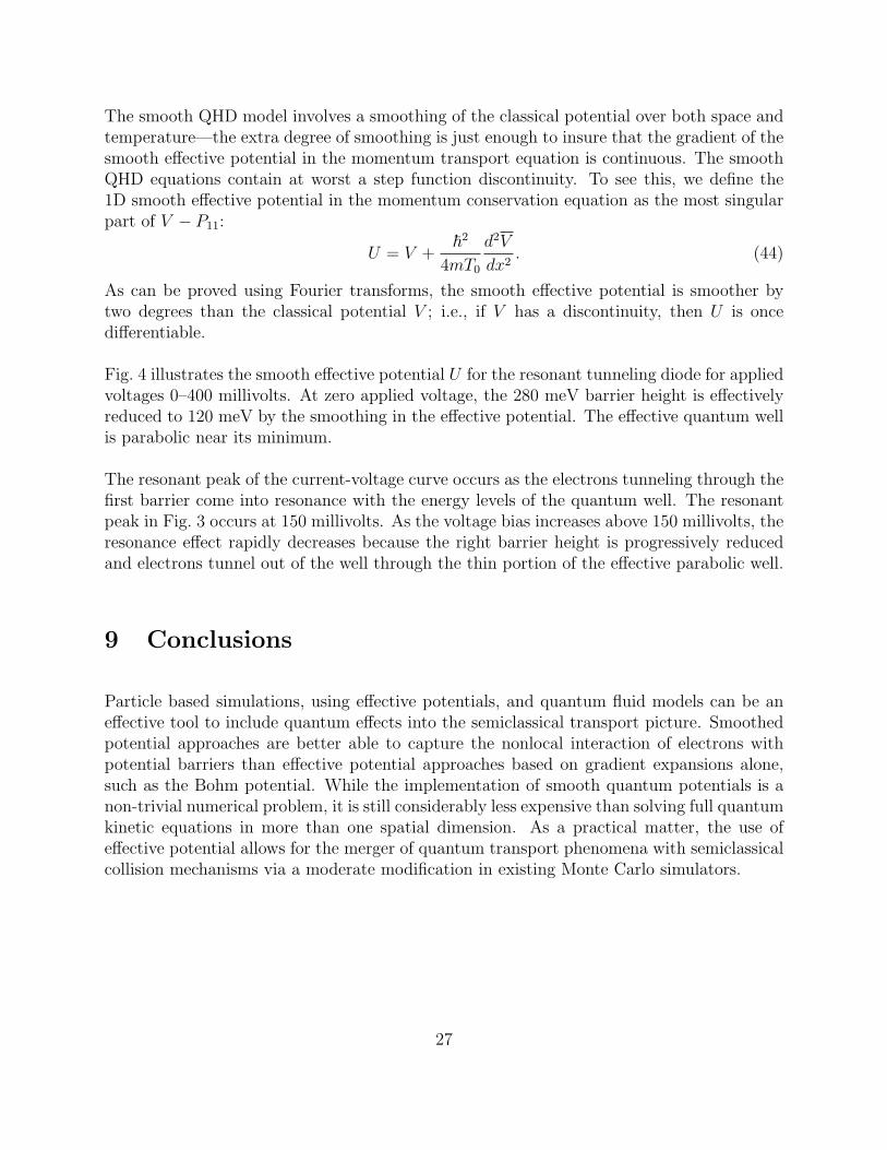
The smooth QHD model involves a smoothing of the classical potential over both space andtemperature—the extra degree of smoothing is just enough to insure that the gradient of thesmooth effective potential in the momentum transport equation is continuous. The smoothQHD equations contain at worst a step function discontinuity. To see this, we define the1D smooth effective potential in the momentum conservation equation as the most singularpart of V − P11:

U = V +~2

4mT0

d2V

dx2. (44)

As can be proved using Fourier transforms, the smooth effective potential is smoother bytwo degrees than the classical potential V ; i.e., if V has a discontinuity, then U is oncedifferentiable.

Fig. 4 illustrates the smooth effective potential U for the resonant tunneling diode for appliedvoltages 0–400 millivolts. At zero applied voltage, the 280 meV barrier height is effectivelyreduced to 120 meV by the smoothing in the effective potential. The effective quantum wellis parabolic near its minimum.

The resonant peak of the current-voltage curve occurs as the electrons tunneling through thefirst barrier come into resonance with the energy levels of the quantum well. The resonantpeak in Fig. 3 occurs at 150 millivolts. As the voltage bias increases above 150 millivolts, theresonance effect rapidly decreases because the right barrier height is progressively reducedand electrons tunnel out of the well through the thin portion of the effective parabolic well.

9 Conclusions

Particle based simulations, using effective potentials, and quantum fluid models can be aneffective tool to include quantum effects into the semiclassical transport picture. Smoothedpotential approaches are better able to capture the nonlocal interaction of electrons withpotential barriers than effective potential approaches based on gradient expansions alone,such as the Bohm potential. While the implementation of smooth quantum potentials is anon-trivial numerical problem, it is still considerably less expensive than solving full quantumkinetic equations in more than one spatial dimension. As a practical matter, the use ofeffective potential allows for the merger of quantum transport phenomena with semiclassicalcollision mechanisms via a moderate modification in existing Monte Carlo simulators.

27

References

[1] R. Akis, S. Milicic, D. K. Ferry,D. Vasileska: An effective potential method for includingquantum effects into the simulation of ultra-short and ultra-narrow channel MOSFETs,Proceedings of the 4th International Conference on Modeling and Simulation of Mi-crosystems, Hilton Head Island, SC, March 19-21, pp. 550-3, 2001.

[2] P. Argyres: Quantum kinetic equations for electrons in high electric and phonon field,Physics Letters, vol. A 171, p. ??, 1992.

[3] G.Baccarani, M. Wordeman: An investigation of steady-state velocity overshoot effectsin Si and GaAs devices, Solid State Electronics, vol. 28, pp. 407–416, 1985.

[4] J.Barker, D. Ferry: Self-scattering path-variable formulation of high-field, time-dependent, quantum kinetic equations for semiconductor transport in the finite collision-duration regime, Physical Review Letters, vol. 42, pp. 1779–1781, 1979.

[5] N. Ben Abdallah, P. Degond,I.M. Gamba: Coupling one-dimensional time-dependentclassical and quantum transport models, J. Math. Phys. 43(1), 1-24, 2002.

[6] P. Degond, S. Mas-Gallic: The Weighted Particle Method for Convection-DiffusionEquations. Part 1: The Case of an Isotropic Viscosity, Mathematics of Computation,Vol. 53, No. 188. , pp. 485-507, 1989.

[7] P. Degond, S. Mas-Gallic: The Weighted Particle Method for Convection-DiffusionEquations. Part 2: The AnisotropicCase, Mathematics of Computation, Vol. 53, No.188, pp. 509-525, 1989.

[8] D. Ferry, H. Grubin: Modelling of quantum transport in semiconductor devices, SolidState Phys. 49 , pp.283–448, 1995 .

[9] D. K. Ferry: First-Order Optical and Intervalley Scattering in Semiconductors, Phys.Rev. B, Vol. 14, 1605, 1976.

[10] F. Fromlet, P. Markowich, C. Ringhofer: A Wignerfunction approach to phonon scat-tering, VLSI Design, vol. 9, p. ??, 1999.

[11] C. Gardner: The quantum hydrodynamic model for semiconductor devices, SIAM Jour-nal on Applied Mathematics, vol. 54, pp. 409–427, 1994.

[12] C. Gardner: Resonant tunneling in the quantum hydrodynamic model, VLSI Design,vol. 3, pp. 201–210, 1995.

[13] C. L. Gardner and C. Ringhofer: Smooth quantum potential for the hydrodynamicmodel Physical Review, vol. E 53, pp. 157–167, 1996.

28

[14] C.Gardner, C.Ringhofer: Approximation of thermal equilibrium for quantum gases withdiscontinuous potentials and application to semiconductor devices, SIAM Journal onApplied Mathematics, vol. 58, pp. 780–805, 1998.

[15] I. Gasser, A. Jungel: The quantum hydrodynamic model for semiconductors in thermalequilibrium, Z. Angew. Math. Phys. 48 , pp. 45–59 ,1997.

[16] I. Gasser, P. Markowich and C. Ringhofer: Closure conditions for classical and quantummoment hierarchies in the small temperature limit, Transp. Th. Stat. Phys. 25 , pp.409–423, 1996.

[17] I. Gasser and P. A. Markowich: Quantum Hydrodynamics, Wigner Transforms and theClassical Limit, Asympt. Analysis, Vol. 14, No. 2, pp. 97-116,1997.

[18] I. Gasser, C.K. Lin,P.A. Markowich: A Review of Dispersive Limits of (non)linearSchrdinger-Type Equations, Taiwanese Journal. of Math., Vol.4, No.4, pp.501-529,2000.

[19] W. J. Gross, D. Vasileska, D. K. Ferry: 3D Simulations of Ultra-Small MOSFETs withReal-Space Treatment of the Electron-Electron and Electron-Ion Interactions, VLSIDesign, Vol. 10, 437, 2000.

[20] R. W. Hockney, J. W. Eastwood: Computer Simulation Using Particles, Maidenhead:McGraw-Hill, 1981.

[21] C. Herring, E. Vogt: Transport and Deformation-Potential Theory for Many-ValleySemiconductors with Anisotropic Scattering, Phys. Rev., Vol. 101, 944, 1956.

[22] C. Jacoboni, L. Reggiani: The Monte Carlo Method for the Solution of Charge Trans-port in Semiconductors with Applications to Covalent Materials, Rev. Modern Phys.,Vol. 55, 645, 1983.

[23] S. E. Laux: On particle-mesh coupling in Monte Carlo semiconductor device simultion,IEEE Trans. CAD Integr. Circ. Syst. , Vol. 15, 1266, 1996.

[24] C. Lent, D. Kirkner: The quantum tranmitting boundary method, Journal of AppliedPhysics, vol 67, pp.6353-6359, 1990.

[25] E. Polizzi, N. Ben Abdallah: Self-consistent three dimensional models for quan-tum ballistic transport in open systems, submitted, URL: http://www.math.tu-berlin.de/ tmr/preprint/authors.html, 2002.

[26] E. Polizzi, N. Ben Abdallah: Space lateral transfer and negative differential conductanceregimes in quantum waveguide junctions, to appear in Journal of Applied Physics, URL:http://www.math.tu-berlin.de/ tmr/preprint/authors.html, 2000.

29

[27] S. Ramey, D. Ferry: Modeling of quantum effects in ultrasmall FD-SOI MOS-FETs with effective potentials and 3D Monte Carlo, Physica B, in press, URL:http://www.eas.asu.edu/ ferry/quantumdev.htm, 2002.

[28] C. Ringhofer: Computational methods for semiclassical and quantum transport in semi-conductor devices, Acta Numerica, vol. 3, pp. 485–521, 1997.

[29] L. Shifren, C. Ringhofer, D.Ferry: A Wigner function based quantum ensemble MonteCarlo study of a resonant tunneling diode, to appear, IEEE Electron Device Letters,URL: http://math.la.asu.edu/ chris , 2002.

[30] L. Shifren, D. Ferry: Particle Monte Carlo simulation of Wigner function tunneling,Physics Letters A 285, 217-221,2001.

[31] E. Wigner: On the quantum correction for thermodynamic equilibrium, Physical Re-view, vol. 40, pp. 749–759, 1932.

[32] R. E. Wyatt: Quantum Wavepacket Dynamics with Trajectories: Wavefunction Syn-thesis along Quantum Paths, Chem. Phys. Lett. 313, 189-197 , 1999.

[33] R. E. Wyatt: Quantum Wave Packet Dynamics with Trajectories: Application to Re-active Scattering, J. Chem. Phys. 111, 4406-4413, 1999.

30