EE3202BJT AC Analysis

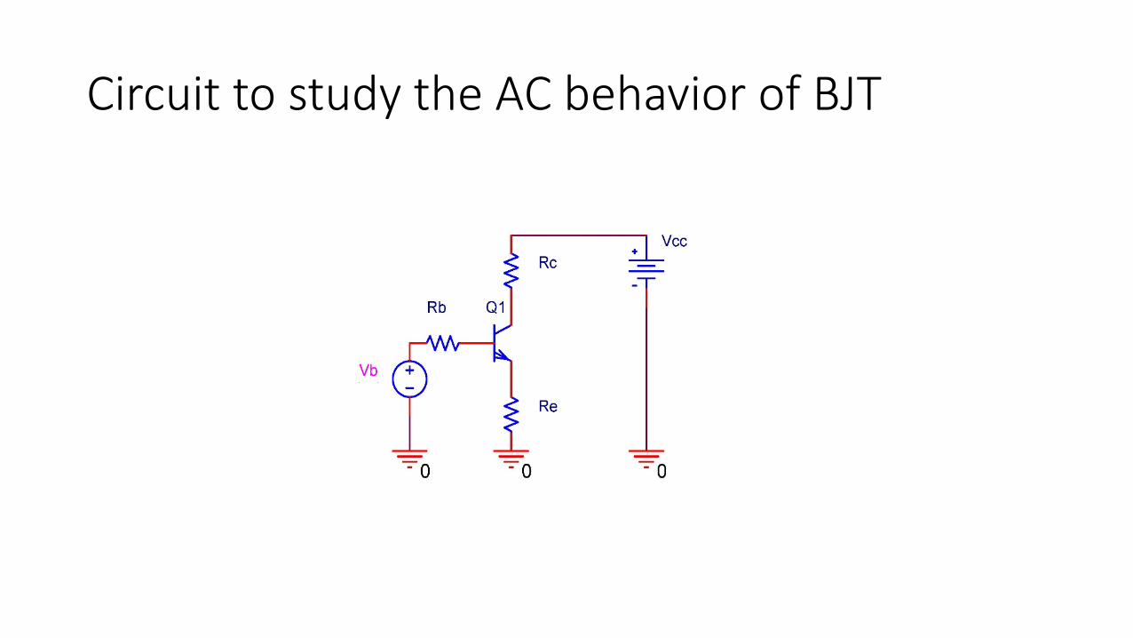
Circuit to study the AC behavior of BJT

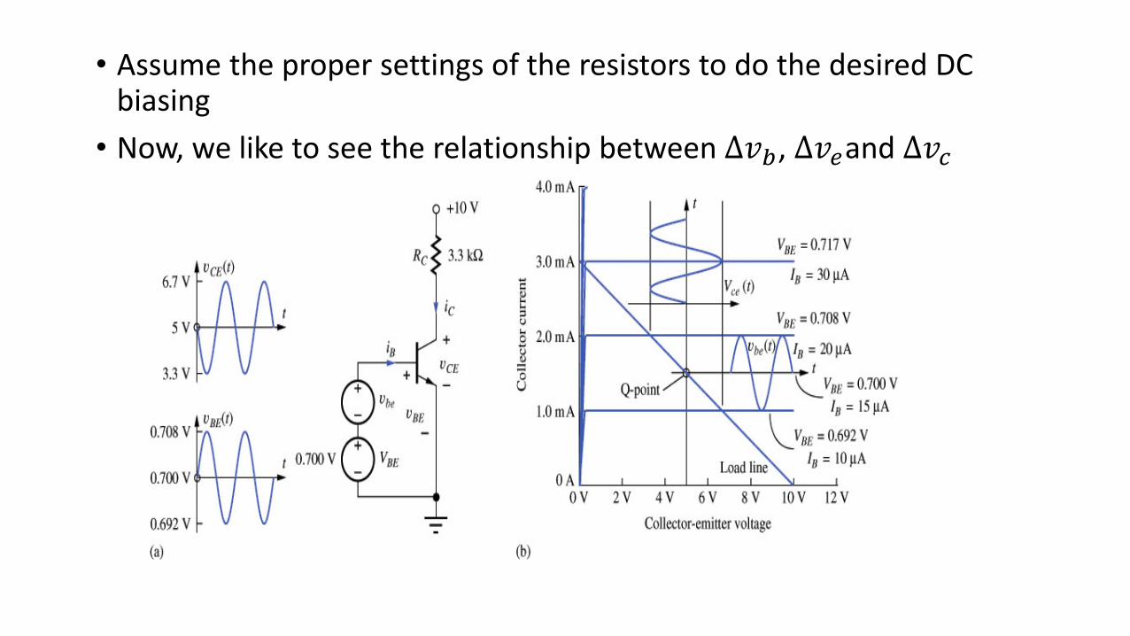
• Assume the proper settings of the resistors to do the desired DC biasing

• Now, we like to see the relationship between Δ𝑣𝑣𝑏𝑏, Δ𝑣𝑣𝑒𝑒and Δ𝑣𝑣𝑐𝑐

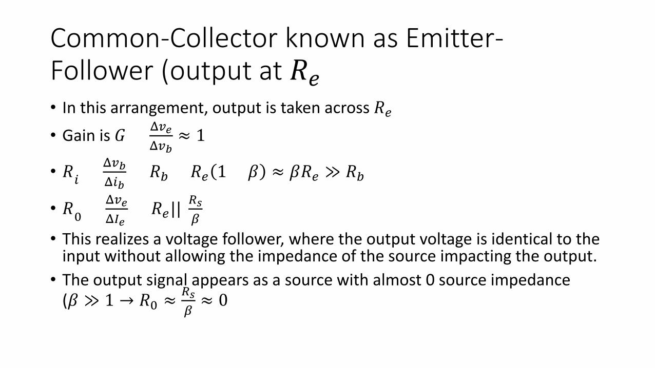
Common-Collector known as Emitter-Follower (output at 𝑅𝑅𝑒𝑒)• In this arrangement, output is taken across 𝑅𝑅𝑒𝑒• Gain is 𝐺𝐺 = Δ𝑣𝑣𝑒𝑒

Δ𝑣𝑣𝑏𝑏≈ 1

• 𝑅𝑅𝑖𝑖 = Δ𝑣𝑣𝑏𝑏Δ𝑖𝑖𝑏𝑏

= 𝑅𝑅𝑏𝑏 + 𝑅𝑅𝑒𝑒 1 + 𝛽𝛽 ≈ 𝛽𝛽𝑅𝑅𝑒𝑒 ≫ 𝑅𝑅𝑏𝑏

• 𝑅𝑅0 = Δ𝑣𝑣𝑒𝑒Δ𝐼𝐼𝑒𝑒

= 𝑅𝑅𝑒𝑒|| 𝑅𝑅𝑠𝑠𝛽𝛽

• This realizes a voltage follower, where the output voltage is identical to the input without allowing the impedance of the source impacting the output.

• The output signal appears as a source with almost 0 source impedance (𝛽𝛽 ≫ 1 → 𝑅𝑅0 ≈

𝑅𝑅𝑠𝑠𝛽𝛽≈ 0)

Common-Emitter (output from 𝑅𝑅𝐶𝐶)

• Gain=Δ𝑣𝑣𝑐𝑐Δ𝑣𝑣𝑏𝑏

= − 𝛽𝛽1+𝛽𝛽

× 𝑅𝑅𝑐𝑐𝑅𝑅𝑒𝑒≈ − 𝑅𝑅𝑐𝑐

𝑅𝑅𝑒𝑒(good amplification can be realized)

• What if 𝑅𝑅𝑒𝑒 = 0? The gain is not infinite!

• We must consider the intrinsic emitter impedance 𝑖𝑖𝑒𝑒 = 𝐼𝐼0 𝑒𝑒𝑞𝑞𝑣𝑣𝐵𝐵𝐵𝐵𝐾𝐾𝑏𝑏𝑇𝑇 − 1

• 𝑟𝑟𝑒𝑒 = Δ𝑣𝑣𝐵𝐵𝐵𝐵Δ𝑖𝑖𝑒𝑒

≈ 26𝐼𝐼𝑒𝑒 𝑚𝑚𝑚𝑚

Ω (at room temperature)

• Gain= Δ𝑣𝑣𝑐𝑐Δ𝑣𝑣𝑏𝑏

≈ −𝑅𝑅𝑐𝑐𝑟𝑟𝑒𝑒

• 𝑅𝑅𝑜𝑜 = Δ𝑣𝑣𝑐𝑐Δ𝐼𝐼𝑐𝑐

= 𝑅𝑅𝑐𝑐• 𝑅𝑅𝑖𝑖 ≈ 𝛽𝛽𝑅𝑅𝑒𝑒

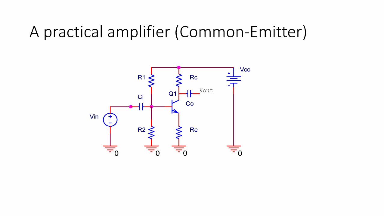
A practical amplifier (Common-Emitter)

• This circuit must be biased using DC analysis of the last experiment• Since we have an option on choosing collector or emitter resistances, the

gain can be set (see example 1 of the Introduction)• Once all the resistors are determined, we need to find the DC blocking

capacitors at the input and output• The input impedance of the circuit (note that you have to ground all

supply voltages to do AC analysis) is 𝑅𝑅1,𝑅𝑅2, 𝑎𝑎𝑎𝑎𝑎𝑎 𝑅𝑅𝑖𝑖 all in parallel• 𝑅𝑅𝑖𝑖 = 𝛽𝛽𝑅𝑅𝑒𝑒 is the input impedance of the common emitter amplifier• If we desire a corner frequency of 𝑓𝑓𝑖𝑖 (this is the lower bound of the

operating frequency of the amplifier), then

𝑓𝑓𝑖𝑖 =1

2𝜋𝜋(𝑅𝑅1 𝑅𝑅2 𝑅𝑅𝑖𝑖)𝐶𝐶𝑖𝑖

• 𝐶𝐶𝑜𝑜 can be found using 𝑓𝑓𝑜𝑜 = 12𝜋𝜋 𝑅𝑅𝑐𝑐+𝑅𝑅𝑙𝑙𝑙𝑙𝑙𝑙𝑙𝑙 𝐶𝐶0

where 𝑓𝑓𝑜𝑜 is AC coupling frequency (which may be different from 𝑓𝑓𝑖𝑖)

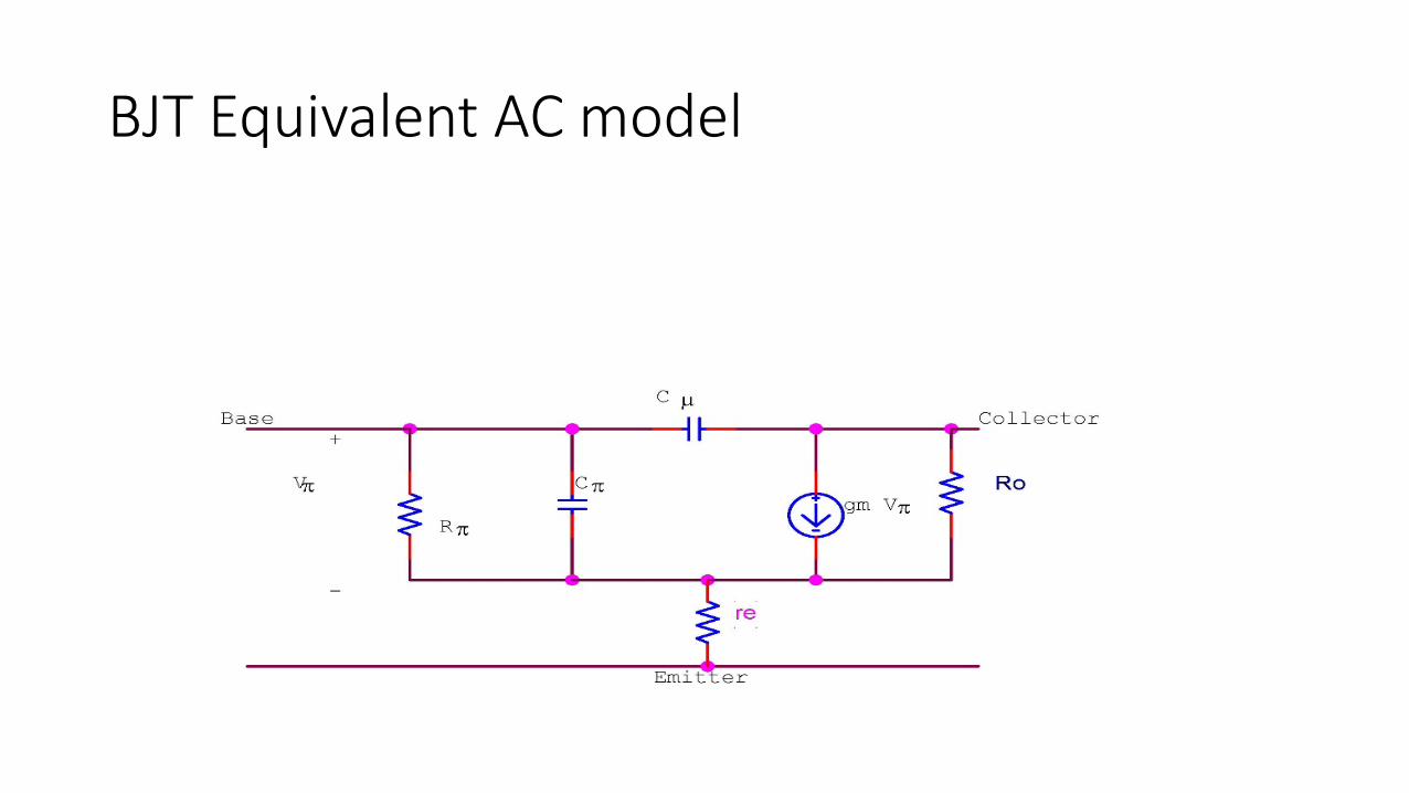
BJT Equivalent AC model

• 𝑔𝑔𝑚𝑚 = 𝑖𝑖𝑐𝑐𝑉𝑉𝑇𝑇≈ 40𝑖𝑖𝑐𝑐 (𝑉𝑉𝑇𝑇 ≈ 0.025)

• 𝑅𝑅𝜋𝜋 = 𝛽𝛽𝑔𝑔𝑚𝑚

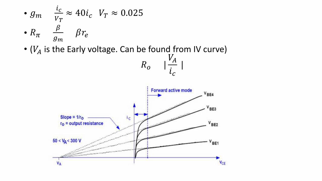
= 𝛽𝛽𝑟𝑟𝑒𝑒• (𝑉𝑉𝑚𝑚 is the Early voltage. Can be found from IV curve)

𝑅𝑅𝑜𝑜 = |𝑉𝑉𝑚𝑚𝑖𝑖𝑐𝑐

|

• 𝐶𝐶𝜇𝜇 𝑎𝑎𝑎𝑎𝑎𝑎 𝐶𝐶𝜋𝜋 can be found from the datasheet.• Once can perform an AC analysis (small signal) using the equivalent

model. • The validity of such model depends on the signal range, frequency,

and accuracy of the components used.• It is best to use PSpice to validate your analysis. • One application of BJT is in realization of differential amplifiers• Such amplifier can be used to realize various analog signal processing

(such as integration, differentiation, addition, subtraction, etc.)

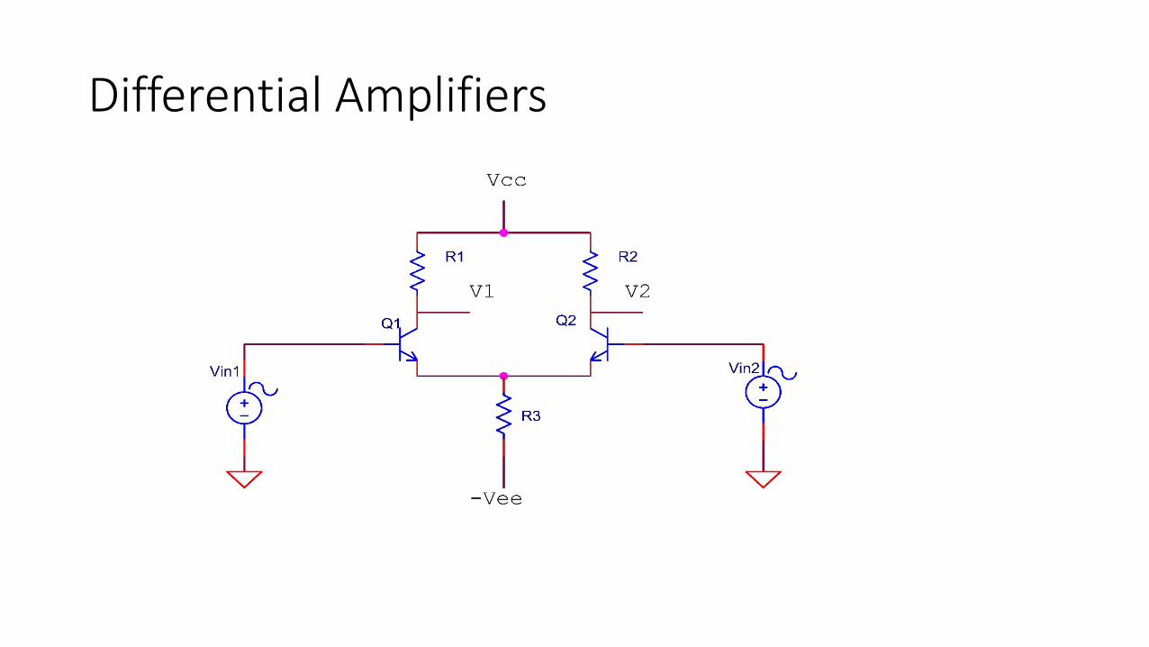
Differential Amplifiers

Differential Amplifier Types and Performance• Single Input Balanced Output (SIBO)• Single Input unbalanced Output (SIUO)• Double Input Balanced Output (DIBO)• Double Input unbalanced Output (DIUO)• DIBO is the most common scenario (as it allows comparing two signals)• For 𝑅𝑅1 = 𝑅𝑅2 = 𝑅𝑅𝐿𝐿, 𝑟𝑟𝑒𝑒1 = 𝑟𝑟𝑒𝑒2 = 𝑟𝑟𝑒𝑒, 𝑅𝑅𝑠𝑠𝑠

𝛽𝛽& 𝑅𝑅𝑠𝑠𝑠

𝛽𝛽≪ 𝑅𝑅3 & 𝑟𝑟𝑒𝑒

• 𝑉𝑉𝑜𝑜𝑜𝑜𝑜𝑜 = 𝑅𝑅𝐿𝐿𝑟𝑟𝑒𝑒

𝑉𝑉𝑖𝑖𝑖𝑖1 − 𝑉𝑉𝑖𝑖𝑖𝑖2 → 𝑔𝑔𝑎𝑎𝑖𝑖𝑎𝑎 = 𝑅𝑅𝐿𝐿𝑟𝑟𝑒𝑒

• 𝑅𝑅𝑖𝑖𝑖𝑖1 = 𝑅𝑅𝑖𝑖𝑖𝑖2 = 2𝛽𝛽𝑟𝑟𝑒𝑒• 𝑅𝑅𝑜𝑜𝑜𝑜𝑜𝑜 = 𝑅𝑅𝐿𝐿• 𝐹𝐹𝐹𝐹𝑟𝑟 𝐷𝐷𝐶𝐶 𝑏𝑏𝑖𝑖𝑎𝑎𝑏𝑏𝑖𝑖𝑎𝑎𝑔𝑔 𝑖𝑖𝑒𝑒 = 𝑖𝑖𝑐𝑐 = 𝑉𝑉𝑒𝑒𝑒𝑒−𝑉𝑉𝐵𝐵𝐵𝐵

2𝑅𝑅3, 𝑉𝑉𝐶𝐶𝐶𝐶 = 𝑉𝑉𝐶𝐶𝐶𝐶 + 𝑉𝑉𝐵𝐵𝐶𝐶 − 𝑅𝑅𝐿𝐿𝑖𝑖𝑐𝑐

Current Mirrors

𝐼𝐼𝑅𝑅𝐶𝐶𝑅𝑅𝐼𝐼𝑜𝑜

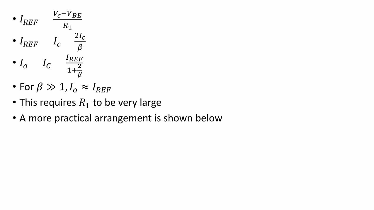
• 𝐼𝐼𝑅𝑅𝐶𝐶𝑅𝑅 = 𝑉𝑉𝑐𝑐−𝑉𝑉𝐵𝐵𝐵𝐵𝑅𝑅𝑠

• 𝐼𝐼𝑅𝑅𝐶𝐶𝑅𝑅 = 𝐼𝐼𝑐𝑐 + 2𝐼𝐼𝑐𝑐𝛽𝛽

• 𝐼𝐼𝑜𝑜 = 𝐼𝐼𝐶𝐶 = 𝐼𝐼𝑅𝑅𝐵𝐵𝑅𝑅1+𝑠𝛽𝛽

• For 𝛽𝛽 ≫ 1, 𝐼𝐼𝑜𝑜 ≈ 𝐼𝐼𝑅𝑅𝐶𝐶𝑅𝑅• This requires 𝑅𝑅1 to be very large• A more practical arrangement is shown below

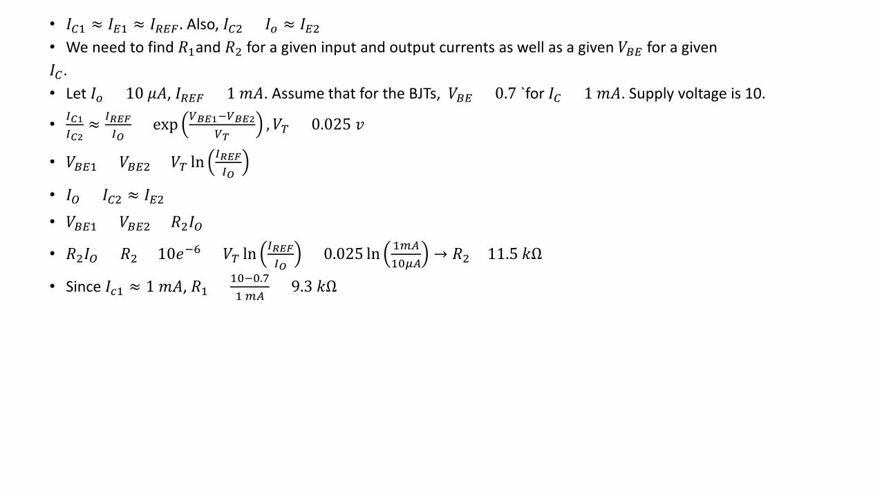
• 𝐼𝐼𝐶𝐶1 ≈ 𝐼𝐼𝐶𝐶1 ≈ 𝐼𝐼𝑅𝑅𝐶𝐶𝑅𝑅 . Also, 𝐼𝐼𝐶𝐶2 = 𝐼𝐼𝑜𝑜 ≈ 𝐼𝐼𝐶𝐶2• We need to find 𝑅𝑅1and 𝑅𝑅2 for a given input and output currents as well as a given 𝑉𝑉𝐵𝐵𝐶𝐶 for a given 𝐼𝐼𝐶𝐶.• Let 𝐼𝐼𝑜𝑜 = 10 𝜇𝜇𝜇𝜇, 𝐼𝐼𝑅𝑅𝐶𝐶𝑅𝑅 = 1 𝑚𝑚𝜇𝜇. Assume that for the BJTs, 𝑉𝑉𝐵𝐵𝐶𝐶 = 0.7 `for 𝐼𝐼𝐶𝐶 = 1 𝑚𝑚𝜇𝜇. Supply voltage is 10.

• 𝐼𝐼𝐶𝐶𝑠𝐼𝐼𝐶𝐶𝑠

≈ 𝐼𝐼𝑅𝑅𝐵𝐵𝑅𝑅𝐼𝐼𝑂𝑂

= exp 𝑉𝑉𝐵𝐵𝐵𝐵𝑠−𝑉𝑉𝐵𝐵𝐵𝐵𝑠𝑉𝑉𝑇𝑇

,𝑉𝑉𝑇𝑇 = 0.025 𝑣𝑣

• 𝑉𝑉𝐵𝐵𝐶𝐶1 = 𝑉𝑉𝐵𝐵𝐶𝐶2 + 𝑉𝑉𝑇𝑇 ln 𝐼𝐼𝑅𝑅𝐵𝐵𝑅𝑅𝐼𝐼𝑂𝑂

• 𝐼𝐼𝑂𝑂 = 𝐼𝐼𝐶𝐶2 ≈ 𝐼𝐼𝐶𝐶2• 𝑉𝑉𝐵𝐵𝐶𝐶1 = 𝑉𝑉𝐵𝐵𝐶𝐶2 + 𝑅𝑅2𝐼𝐼𝑂𝑂

• 𝑅𝑅2𝐼𝐼𝑂𝑂 = 𝑅𝑅2 × 10𝑒𝑒−6 = 𝑉𝑉𝑇𝑇 ln 𝐼𝐼𝑅𝑅𝐵𝐵𝑅𝑅𝐼𝐼𝑂𝑂

= 0.025 ln 1𝑚𝑚𝑚𝑚10𝜇𝜇𝑚𝑚

→ 𝑅𝑅2= 11.5 𝑘𝑘Ω

• Since 𝐼𝐼𝑐𝑐1 ≈ 1 𝑚𝑚𝜇𝜇, 𝑅𝑅1 = 10−0.71𝑚𝑚𝑚𝑚

= 9.3 𝑘𝑘Ω