Education and Signaling: Evidence from a

Highly Competitive Labor Market in 2001

By

LO FAN

03005445

Applied Economic Option

An Honours Degree Project Submitted to the School of Business in

Partial fulfillment Of the Graduation Requirement for the Degree of

Bachelor of Business Administration (Honours)

Hong Kong Baptist University

Hong Kong

April 2006

1

Acknowledgements

I would like to thank God for helping me to finish this honor project. I forgot how

many times I prayed for help from God. God listened to almost my every prayer.

In the process of doing this honor project, I learnt to be humble, since God remind me

many times. Second, I understand myself and God better. Third, I experienced to have

faith in God is very important in my life. When I try to have faith in God, God gave

the Lambda to me. And I will not forget how excited I was when I got the Lambda by

help from God. Fourth, I learnt to persist until the last moment, by the experience of

doing this honor project, I discovered that the breakthroughs always happen at last

moment. Fifth, I felt care and love from my classmates, supervisor and those from the

church. I learnt and experienced so many things during doing this honor projects. As a

result, I thank God for giving me opportunities to do this honor project. I also thank

God for giving me “difficulties” when I do the honor project, the purpose of these

“difficulties” is to push me to learn new things.

Last but not least, I thank God for giving me my supervisor, Professor, Joanna Kit

Chun LAM, she devoted so much time and effort in helping me to solve the problems.

And the experiences of doing this honor project would probably become one of the

memories in my life.

2

Abstract:

In this study, I found that the educational earnings for the employed are greater than

the self-employed. It can be concluded that it is in 2001, after the Hong Kong

handover, education continues to play a signaling role. And it supports the weak

screening hypothesis, but not strong screening hypothesis. Moreover, the higher

education returns for those completed the course than the dropouts are at least partly

due to signaling value of educational credentials.

3

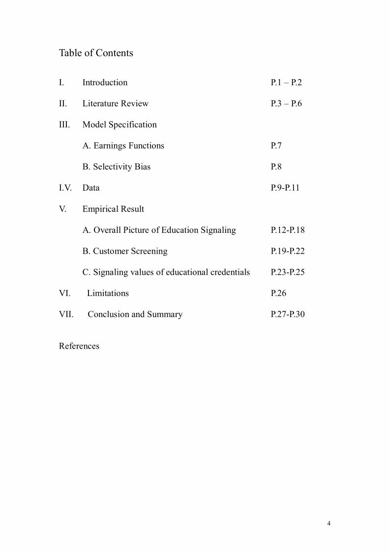
Table of Contents I. Introduction P.1 – P.2 II. Literature Review P.3 – P.6 III. Model Specification A. Earnings Functions P.7

B. Selectivity Bias P.8

I.V. Data P.9-P.11 V. Empirical Result

A. Overall Picture of Education Signaling P.12-P.18

B. Customer Screening P.19-P.22

C. Signaling values of educational credentials P.23-P.25 VI. Limitations P.26 VII. Conclusion and Summary P.27-P.30 References

4

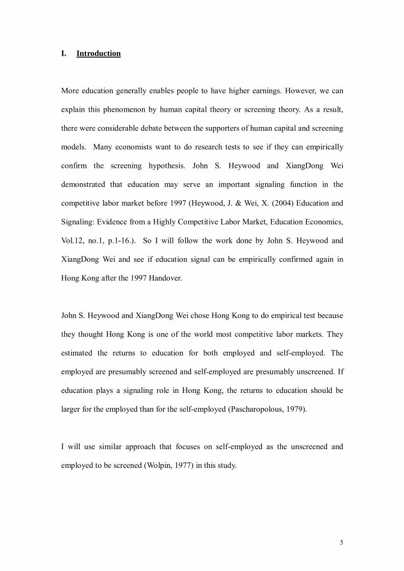
I. Introduction

More education generally enables people to have higher earnings. However, we can

explain this phenomenon by human capital theory or screening theory. As a result,

there were considerable debate between the supporters of human capital and screening

models. Many economists want to do research tests to see if they can empirically

confirm the screening hypothesis. John S. Heywood and XiangDong Wei

demonstrated that education may serve an important signaling function in the

competitive labor market before 1997 (Heywood, J. & Wei, X. (2004) Education and

Signaling: Evidence from a Highly Competitive Labor Market, Education Economics,

Vol.12, no.1, p.1-16.). So I will follow the work done by John S. Heywood and

XiangDong Wei and see if education signal can be empirically confirmed again in

Hong Kong after the 1997 Handover.

John S. Heywood and XiangDong Wei chose Hong Kong to do empirical test because

they thought Hong Kong is one of the world most competitive labor markets. They

estimated the returns to education for both employed and self-employed. The

employed are presumably screened and self-employed are presumably unscreened. If

education plays a signaling role in Hong Kong, the returns to education should be

larger for the employed than for the self-employed (Pascharopolous, 1979).

I will use similar approach that focuses on self-employed as the unscreened and

employed to be screened (Wolpin, 1977) in this study.

5

The weak screening hypothesis (WSH) assumes all individual workers, employed

and self-employed invest in education for increasing their productivities (human

capital theory). Education not only increases the productivities of the employed, it

also signals the employed inherent productivities. So the employed invest in education

for these two reasons. Self-employed do not need to signal their productivities. The

earnings for the self-employed can purely reflect education’s direct influence on

productivity rather than the signaling function of education (Brown & Sessions, 1999).

I will present my study in the following sequence. Section 2 reviews the previous

literature. Section 3 will be the model specification. Section 4 discusses the data.

Section 5 presents empirical result. Section 6 discusses the limitations and Section 7

draws the conclusions.

First, after dealing with the sample selection bias, I do the ordinary least squares (OLS)

estimates for the employed and self-employed. Then I estimate the returns separately

by gender. Second, I take customer screening into account, so I remove all the doctors

and lawyers from the sample, and then I run the earnings regression again by gender.

Finally, I find out the distinction of returns between those completed the course and

those dropouts.

6

II. Literature Review

According to human capital theory, education increases one’s productivity (Becker,

1975). In contrast, screening hypothesis give evidence that education only signals

inherent productivity. And there are two kinds of screening hypothesis, namely, strong

screening hypothesis (SSH) and weak screening hypothesis (WSH).

The strong screening hypothesis (SSH) presumes that productivity has no relationship

with education, and education is only used for screening (Psacharopoulos, 1979). The

weak screening hypothesis (WSH) admitted education increases inherent productivity,

and the primary role of education is to signal inherent productivity. According to the

signaling theories of Arrow (1973), Spence (1974), and Stiglitz (1975), since

education is used to signal inherent productivity, those with higher ability will invest

more in education. It is because they want to use education to signal their higher

capability.

Most common and fundamental test is to examine the differences in returns to

education between a group of workers presumed to be screened and a group presumed

not to be screened, such as those done by Wolpin in 1977 and Riley in 1979. The

prevalent paper follows this tradition (Heywood & Wei, 2004).

Many studies compared the returns to education in presumably screened and

unscreened sectors of economies from all over the world (see Belfield, 2000). Some

compared returns of self-employed and employed, some compared the returns of

those employed by private firms and those employed by governments. There are even

7

some to examine the return to educational attainment, not returns to education.

However, the reason is the same. If education does not act as a signal of productivity

for the self- employed, the self-employed will invest less in education (Heywood &

Wei, 2004).

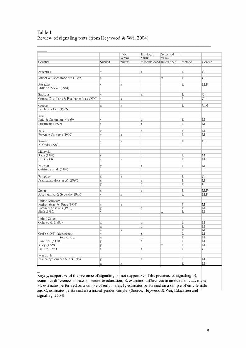
Table 1 provides a summary of about 30 tests using sectoral comparison across

different countries (Heywood & Wei, 2004). From these tests, we cannot draw any

generalization. And Brown & Session concluded that “the extent to which education

is used as a screen depends critically upon the nature of indigenous cultures and

institutions” (Brown & Sessions, 1999, p. 398).

Culture and institutions affect the signaling effect of education in different countries,

and a highly regulated labor market has less individual variation in earnings

(Heywood & Wei, 2004). For example, for the highly corporatist countries of

continental Europe, centrally determined earnings are passed on to all employees in

private sector (see Slomp, 1996). The dispersion of earnings in these countries is

much less than in those with less regulated labor markets (see Addison & Siebert,

1997, Table 10.5).The smaller earnings dispersion in less competitive labor markets

proof that there is less signaling in these markets(Heywood & Wei, 2004).

8

9

Table 1 Review of signaling tests (from Heywood & Wei, 2004) U__________________________________________________________________________U

Public Employed Screened versus versus versus

Country Support private self-employed unscreened Method Gender

Argentina y x R C

Kugler & Psacharopolous (1989) n x R C

Australia y x R M,FMiller & Volker (1984)

Equador y x R C

Gomez-Castellans & Psacharopolous (1990) n x R C

Greece n x R C,MLambropoulous (1992)

IsraelKatz & Zimermann (1980) y x E M

Zidermann (1992) n x R M

Italy y x R MBrown & Sessions (1999) y x R M

Kuwait n x R CAl-Qudsi (1989)

MalaysiaSoon (1987) y x R MLee (1980) n x R M

Pakistan y x R MGuisinger et al. (1984)

Paraguay n x R CPsacharopoulous et al. (1994) n x R M

y x R F

Spain n x R M,FAlba-ramirez & Segundo (1995) y x R M,F

United KingdomArabshiebani & Rees (1997) n x R MBrown & Sessions (1998) y x R MShah (1985) y x R M

United StatesCohn et al. (1987) n x E M

n x R Mn x R M

Grubb (1993) (highschool) y x R M (university) n x R MHamilton (2000) y x R M

Riley (1979) y x R MTucker (1985) n x R C

VenezuelaPsacharopolous & Steier (1988) y x R M

n x R M

U_ Key: y, supportive of the presence of signaling; n, not supportive of the presence of signaling; R, examines differences in rates of return to education; E, examines differences in amounts of education; M, estimates performed on a sample of only males, F, estimates performed on a sample of only female and C, estimates performed on a mixed gender sample. (Source: Heywood & Wei, Education and signaling, 2004)

Two examples can be cited: in United States, Heywood in 1994 found that signaling

only exists in private non-unionized sector of the workforce. And signaling does not

exist in private unionized sector and in all government sectors. Besides, Heywood

found that when the labor market for the employed is more competitive and flexible, a

greater difference in earnings might be expected. Muhlau and Horgan in 2000 found

that US and UK have greater dispersion in earnings and educational signals than

continental Europe. In addition, in US and UK, the correlations between skills

requirements of the jobs and educational signals are greater than continental Europe.

To conclude, educational signals are more significant in a more competitive labor

markets.

10

11

III. U Model Specification

A. Earnings Functions

The following Mincerian earnings equation was estimated for the individual workers:

Lnmearn = α + βB1 Be + βB2 Bx + βB3 BxP

2P + βB4 Bm + βB5 Bi + ε

Where Lnmearn = log monthly earnings, α = average wage for reference respondent, e

= educational level dummy, x = years of labor market experience (proxied by age),

and m = marital status, i = industrial dummy variables. The education level dummies

in vector e denote the respondent’s highest level of education, namely: (1) primary

education, (2) lower secondary education, (3) upper secondary education, (4) post

secondary education, (5) university education. The term ε is included to capture

random errors. The education level dummies in vector i denote industries in which the

respondent work during the seven days before the census moment, namely, (1)

agriculture and fishing, (2) manufacturing, (3) electricity, gas and water, (4)

construction, (5) wholesale and retail, (6) transport, storage and communication, (7)

Financing, insurance, real estate, (8) community, social and personal services, (9) not

classified.

B. Selectivity Bias

Men and women can choose to be employed and self-employed. The choice is not

random. And it depends on which economic activities status enables them have

highest earnings. Some workers have characteristics that make them more likely to be

the self-employed workers. Then the estimated returns to different educational level

will be affected by this sample selection bias. We can deal with this bias by using

method suggested by Heckman (1979). Heckman two-step technique can enable us to

create the inverse mill ratio (Lambda) from the first stage probit. And the inverse

mills ratio (Lambda) is included in the corrected earnings equations (Le, 1999). If the

coefficient for the Lambda is negative, it means there is positive correlation between

the choice functions and the earnings function (Wong, 1986).

12

13

IV. U Data

The data used in this study are from the sample of the 2001 Census. It provides the

variables such as age, its square, gender, marital status of the individual worker, and 8

dummy variables for broad industry of employment. From this data set, no one was

come from mining and quarrying industry. The individual workers are at the age

between 15 and 60 years old. Table 2 is the definitions of data. 2001 Census also

provides the information that whether the individual workers are employed or self-

employed.

Table. 2

Data definitions

Variable name Description

Lnmearn Log monthly earnings

Age Respondent's age in years

Married Respondent is married

Primary Respondent has either no formal education or primary school education

Lower Secondary Respondent has Form 1 to Form 3 education

Upper Secondary Respondent has Form 3 to Form 7 or craft level education

Post Secondary Respondent has post secondary education e.g. diplomas or certificates

University Respondent has either degree, postgraduate education in University

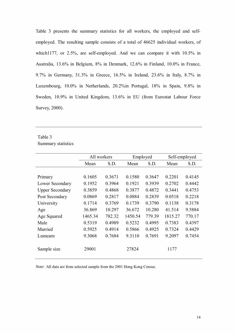
Table 3 presents the summary statistics for all workers, the employed and self-

employed. The resulting sample consists of a total of 46625 individual workers, of

which1177, or 2.5%, are self-employed. And we can compare it with 10.5% in

Australia, 13.6% in Belgium, 8% in Denmark, 12.6% in Finland, 10.0% in France,

9.7% in Germany, 31.3% in Greece, 16.5% in Ireland, 23.6% in Italy, 8.7% in

Luxembourg, 10.0% in Netherlands, 20.2%in Portugal, 18% in Spain, 9.8% in

Sweden, 10.9% in United Kingdom, 13.6% in EU (from Eurostat Labour Force

Survey, 2000).

Table 3 Summary statistics All workers Employed Self-employed Mean S.D. Mean S.D. Mean S.D. Primary 0.1605 0.3671 0.1580 0.3647 0.2201 0.4145 Lower Secondary 0.1952 0.3964 0.1921 0.3939 0.2702 0.4442 Upper Secondary 0.3859 0.4868 0.3877 0.4872 0.3441 0.4753 Post Secondary 0.0869 0.2817 0.0884 0.2839 0.0518 0.2218 University 0.1714 0.3769 0.1739 0.3790 0.1138 0.3178 Age 36.869 10.297 36.672 10.280 41.514 9.5884 Age Squared 1465.34 782.32 1450.54 779.39 1815.27 770.17 Male 0.5319 0.4989 0.5232 0.4995 0.7383 0.4397 Married 0.5925 0.4914 0.5866 0.4925 0.7324 0.4429 Lnmearn 9.3068 0.7684 9.3110 0.7691 9.2097 0.7454 Sample size 29001 27824 1177

Note: All data are from selected sample from the 2001 Hong Kong Census.

14

For the employed, the average age 37 years old, that 52.3% of the employed are male

and 58.7% of the employed are married.

For the self-employed, the average age is 42 years old, which 73.8% of the self-

employed is male and 73.2% of the self-employed are married.

The average natural log of earnings for the employed is 9.31, approximately 11.63%

higher than that for the self-employed at 9.20.

The summary statistics shows that proportion of self-employed with lower education

level is higher than that for the employed. For instance, 35% of the employed have

attained lower secondary or less while the same statistics for the self-employed is

49%. These results coincide with the screening hypothesis that the self-employed are

less concerned and so less interested in investing in education. So they invest less in

education (Wolpin, 1977).

15

16

V. UEmpirical Result

A. Overall Picture of Education Signaling

Table 4

OLS Estimates of earnings functions

Full sample

Employed Self-employed Difference

Constant 6.3379* 7.1043* -0.7664

(108.51) (21.28)

Age 0.1034* 0.1358* -0.0324

(33.47) (9.18)

Age Squared -0.0012* -0.0016* 0.0004

(-29.67) (-9.16)

Male 0.3014* 0.2506* 0.0508

(27.43) (5.01)

Married 0.0779* 0.0888 -0.0109

(6.474) (1.71)

Lower Secondary 0.2026* 0.0934 0.1092

(13.57) (1.65)

Upper Secondary 0.5615* 0.2885* 0.273

(39.21) (5.06)

Post Secondary 0.9636* 0.458* 0.5056

(47.87) (4.62)

University 1.249* 0.5246* 0.7244

(71.158) (6.57)

Lambda 1.3104* -0.3993* 1.7097

(19.88) (-5.85)

Adjusted R-squared 0.4071 0.2242

Sample size 27824 1177

Note: The earnings functions include dummy variables for 9 broad industries. t-Statistics presented in parentheses. * Statistically significant at the 1% level.

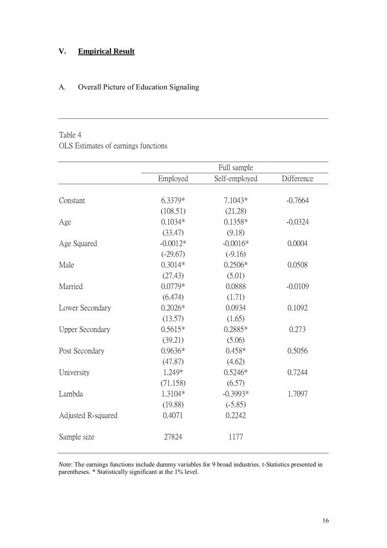
Table 4 presents ordinary least squares (OLS) estimates of the earnings functions for

both employed and self-employed. I corrected for the sample selection bias by

including Lambda in the earnings functions. The estimated coefficient for Lambda for

the employed is significantly positive. On the other hand, the estimated coefficient for

Lambda for the self-employed is significantly negative. It indicates that selection is

not random. And the observed earnings of the self-employed are less than the

population mean, however, the observed earnings of the employed are larger than the

population mean (Wong, 1986, p. 696)

Table 4 shows that age and age-squared are significant in determining the earnings of

employed and self-employed. According to Riley (1979), if the education is an

effective screening device, then is should be an accurate signal of worker productivity.

As a result, the estimated earnings function of employed is expected to fit the data

better than that for the self-employed (Brown & Sessions, 1999, p.400). From table 4,

we can see that around 41% of the variation in employed earnings can be explained

by the regression. On the other hand, it is around 22% of the variation in self-

employed earnings can be explained by the regression. It suggested that the null

hypothesis that there is no evidence of screening is rejected.

The third column of Table 4 presents the difference in the educational returns between

the employed and self-employed. The employed are presumably screened and self-

employed are presumably unscreened. If education plays a signaling role in Hong

Kong, the returns to education should be larger for the employed than for the self-

employed. And from Table 4, we can see that the difference of educational returns

between employed and self-employed is positive at different education levels. The

17

18

higher the education level, the greater the difference is. For lower secondary level, the

difference is 0.1092; for upper secondary, the difference is 0.273; for post secondary,

the difference is 0.5056; for university level, the difference is 0.7244. It is very

obvious that in a higher education level, the signaling effect is greater.

In Table 4 samples of men and women were combined in a single estimate as shown

above. However, the Chow test rejects the null hypothesis that the sectors have same

earnings regression. The Chow tests are as follow:

For employed:

HB0 B: βBmale B= βBfemaleB

HB1 B: βBmale B≠ βBfemale

(RSSBRB – RSSBUR B ) / k F = (RSSBUR B) / (nB1B+ nB2 B- 2k)

(9745 - 9376) / 18 F= 9376 / 27788

F = 60.76

As the computed F value exceeds the critical F value, I reject the null hypothesis of

parameter stability and conclude that the male’s and female’s regression are different.

19

For self-employed:

HB0B: βBmale B= βBfemaleB

HB1 B: βBmale B≠ βBfemale

(RSSBRB – RSSBUR B ) / k F = (RSSBUR B) / (nB1B+ nB2 B- 2k)

(494 - 476) / 16 F= 476 / 1145

F = 2.71

As the computed F value exceeds the critical F value, I reject the null hypothesis of

parameter stability and conclude that the male’s and female’s regression are different.

Table 5 and Table 6 show the educational returns by employment status and estimated

separately for men and women.

The coefficients on the dummies capturing the 8 broad industries are suppressed but

are available from the author.

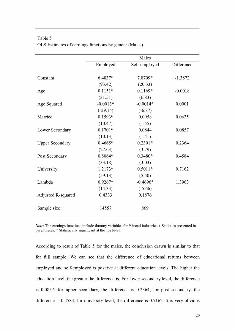
Table 5 OLS Estimates of earnings functions by gender (Males) Males Employed Self-employed Difference Constant 6.4837* 7.8709* -1.3872 (93.42) (20.33) Age 0.1151* 0.1169* -0.0018 (31.51) (6.83) Age Squared -0.0013* -0.0014* 0.0001 (-29.14) (-6.87) Married 0.1593* 0.0958 0.0635 (10.47) (1.55) Lower Secondary 0.1701* 0.0844 0.0857 (10.13) (1.41) Upper Secondary 0.4665* 0.2301* 0.2364 (27.63) (3.79) Post Secondary 0.8064* 0.3480* 0.4584 (33.18) (3.03) University 1.2173* 0.5011* 0.7162 (59.13) (5.50) Lambda 0.9267* -0.4696* 1.3963 (14.33) (-5.66) Adjusted R-squared 0.4333 0.1876 Sample size 14557 869

Note: The earnings functions include dummy variables for 9 broad industries. t-Statistics presented in parentheses. * Statistically significant at the 1% level.

According to result of Table 5 for the males, the conclusion drawn is similar to that

for full sample. We can see that the difference of educational returns between

employed and self-employed is positive at different education levels. The higher the

education level, the greater the difference is. For lower secondary level, the difference

is 0.0857; for upper secondary, the difference is 0.2364; for post secondary, the

difference is 0.4584; for university level, the difference is 0.7162. It is very obvious

20

21

that in a higher education level, the signaling effect is greater.

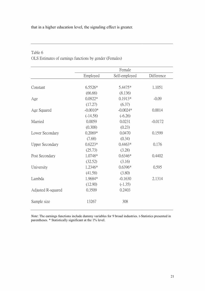
Table 6

OLS Estimates of earnings functions by gender (Females)

Female

Employed Self-employed Difference

Constant 6.5526* 5.4475* 1.1051

(66.66) (8.136)

Age 0.0922* 0.1913* -0.09

(17.27) (6.37)

Age Squared -0.0010* -0.0024* 0.0014

(-14.58) (-6.26)

Married 0.0059 0.0231 -0.0172

(0.308) (0.23)

Lower Secondary 0.2069* 0.0470 0.1599

(7.68) (0.34)

Upper Secondary 0.6223* 0.4463* 0.176

(25.73) (3.28)

Post Secondary 1.0748* 0.6346* 0.4402

(32.52) (3.16)

University 1.2346* 0.6396* 0.595

(41.58) (3.80)

Lambda 1.9684* -0.1630 2.1314

(12.90) (-1.35)

Adjusted R-squared 0.3509 0.2403

Sample size 13267 308

Note: The earnings functions include dummy variables for 9 broad industries. t-Statistics presented in parentheses. * Statistically significant at the 1% level.

According to result of Table 6 for the females, the conclusion drawn is similar to that

for males. We can see that the difference of educational returns between employed

and self-employed is positive at different education levels. The higher the education

level, the greater the difference is. For lower secondary level, the difference is 0.1599;

for upper secondary, the difference is 0.176; for post secondary, the difference is

0.4402; for university level, the difference is 0.595. It is very obvious that in a higher

education level, the signaling effect is greater.

22

B. Customer Screening

I need to modify the assumption that the self-employed are not screened. Since some

self-employed workers are screened, like medical doctors and lawyer. It is the

customers to see their credentials, when one to see the doctors, they would like to

know what qualification did that doctor have, and then decide whether to choose to

see that doctor. It is because the customers don’t have perfect information about the

doctors and lawyers, they just using education attainment as a device to screen

different doctors or lawyers.

In this sense, education serves a signaling function. I follow that modification done by

J.S. Heywood & X. Wei. I remove all the medical doctors and lawyers from the

samples, and then I run the earnings regressions in Table 5 and Table 6 again by

gender. The sample size change a little bit. The original sample size has 14557 males

are employed; 869 males are self-employed; 13267 females are employed; 308

females are self-employed. After removing the doctors and lawyers, the sample size

decreased, there are 14385 males are employed; 853 males are self-employed; 13066

females are employed; 303 females are self-employed.

23

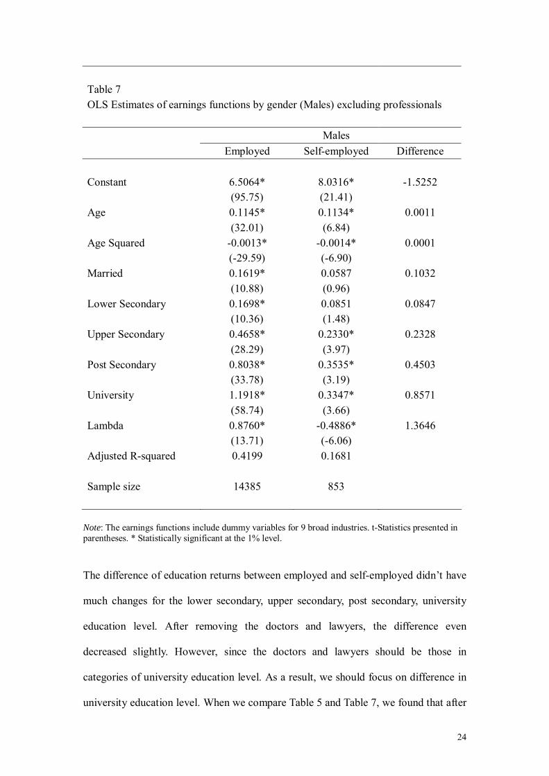
Table 7 OLS Estimates of earnings functions by gender (Males) excluding professionals Males Employed Self-employed Difference Constant 6.5064* 8.0316* -1.5252 (95.75) (21.41) Age 0.1145* 0.1134* 0.0011 (32.01) (6.84) Age Squared -0.0013* -0.0014* 0.0001 (-29.59) (-6.90) Married 0.1619* 0.0587 0.1032 (10.88) (0.96) Lower Secondary 0.1698* 0.0851 0.0847 (10.36) (1.48) Upper Secondary 0.4658* 0.2330* 0.2328 (28.29) (3.97) Post Secondary 0.8038* 0.3535* 0.4503 (33.78) (3.19) University 1.1918* 0.3347* 0.8571 (58.74) (3.66) Lambda 0.8760* -0.4886* 1.3646 (13.71) (-6.06) Adjusted R-squared 0.4199 0.1681 Sample size 14385 853

Note: The earnings functions include dummy variables for 9 broad industries. t-Statistics presented in parentheses. * Statistically significant at the 1% level. The difference of education returns between employed and self-employed didn’t have

much changes for the lower secondary, upper secondary, post secondary, university

education level. After removing the doctors and lawyers, the difference even

decreased slightly. However, since the doctors and lawyers should be those in

categories of university education level. As a result, we should focus on difference in

university education level. When we compare Table 5 and Table 7, we found that after

24

we exclude the doctors and lawyers, the difference of educational returns between

employed and self-employed is even greater. Before removing doctors and lawyers

from sample, the difference of university education returns is 0.7162. However, when

we removed the doctors and lawyers, the difference increased to 0.8571.

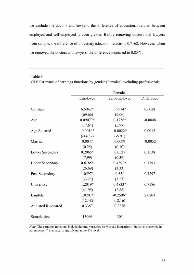
Table 8 OLS Estimates of earnings functions by gender (Females) excluding professionals Females Employed Self-employed Difference Constant 6.5942* 5.9914* 0.6028 (69.66) (9.06) Age 0.09077* 0.1756* -0.0848 (17.64) (5.97) Age Squared -0.0010* -0.0022* 0.0012 (-14.87) (-5.91) Married 0.0047 0.0099 -0.0052 (0.25) (0.10) Lower Secondary 0.2065* 0.0527 0.1538 (7.99) (0.39) Upper Secondary 0.6185* 0.4392* 0.1793 (26.69) (3.33) Post Secondary 1.0597* 0.63* 0.4297 (33.27) (3.23) University 1.2019* 0.4833* 0.7186 (41.95) (2.88) Lambda 1.8207* -0.2596* 2.0803 (12.48) (-2.16) Adjusted R-squared 0.3357 0.2276 Sample size 13066 303

Note: The earnings functions include dummy variables for 9 broad industries. t-Statistics presented in parentheses. * Statistically significant at the 1% level.

25

The same conclusion applied to females’ earnings functions when excluding the

doctors and lawyers. The difference of education returns between employed and self-

employed didn’t have much changes for the lower secondary, upper secondary, post

secondary, university education level. After removing the doctors and lawyers, the

difference even decreased slightly. Again we should focus on difference in university

education level only since the doctors and lawyers should be those in university

education level. When we compare Table 6 and Table 8, we found that after we

exclude the doctors and lawyers, the positive difference of educational returns

between employed and self-employed is even greater. Before removing doctors and

lawyers from sample, the difference of university education returns is 0.595. However,

when we removed the doctors and lawyers, the difference increased to 0.7186.

26

C. Signaling Value of Educational Credentials

2001 Census provides the information about the education attainment of the

individual workers. In total, there are two education attainment variables, namely,

highest level attended and highest level completed.

Highest level attended is defined as the highest level of education ever attained by a

person in school or other institution, regardless of whether he had completed the

course. And the highest level completed is defined as the highest level of education

completed by a person in school or other educational institution, regardless of whether

he had passed the examinations or assessments of the course (2001 Population

Census 1% Sample Data Set-User Guide, 2002).

These two education attainment variables allow us to identify those who attempted an

educational level (such as Form 3) but dropped out (J. S. Heywood & X. Wei, 2004,

p.5-6). Those dropouts attended but didn’t completed the course should earn less than

those attended and also completed the course. It can be explained by human capital

theory, since the dropouts received less education, so their productivity is lower than

those completed the course, it explained why they earn less. And their education

returns are less than those completed the course. However, we cannot deny that those

completed the courses have higher education returns than those drop out is partly due

to the signaling value of educational credentials (J. S. Heywood & X. Wei, 2004,

p.13). That is why J. S. Heywood and X. Wei in 2004 tried to test directly for the

differences in returns between those completed and dropouts (J. S. Heywood & X.

Wei, 2004, p.2)

27

I also want to find out the distinction of returns between those completed the course

and those dropouts. Table 9 presents OLS estimates of earnings functions for

employed, individual workers are grouped in fine categories. This earnings function

shows that earnings increased with additional education. It may partly due to human

capital theory and partly due to signaling value of educational credentials.

28

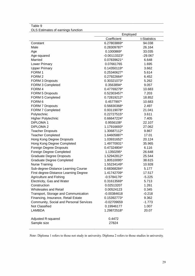
Table 9 OLS Estimates of earnings function Employed Coefficient t-Statistics Constant 6.27803869* 94.038 Male 0.28309787* 26.164 Age 0.1000869* 33.035 Age-squared -0.00113323* -29.067 Married 0.07839621* 6.648 Lower Primary 0.07661765 1.695 Upper Primary 0.14350119* 3.662 FORM 1 0.25340627* 5.614 FORM 2 0.27922664* 6.452 FORM 3 Dropouts 0.30321073* 5.262 FORM 3 Completed 0.3563894* 9.057 FORM 4 0.47769279* 10.683 FORM 5 Dropouts 0.52303457* 7.203 FORM 5 Completed 0.72819212* 18.852 FORM 6 0.4577997* 10.683 FORM 7 Dropouts 0.56830368* 2.497 FORM 7 Completed 0.93119078* 21.041 Polytechnic 0.22727515* 3.611 Higher Polytechnic 0.66647224* 7.405 DIPLOMA 1 0.9556108* 22.107 DIPLOMA 2 1.17916693* 27.062 Teacher Dropouts 1.30687112* 9.867 Teacher Completed 1.64605887* 17.01 Hong Kong Degree Dropouts 1.03931652* 20.124 Hong Kong Degree Completed 1.49770931* 35.965 Foreign Degree Dropouts 0.47324804* 6.116 Foreign Degree Completed 1.1350295* 26.648 Graduate Degree Dropouts 1.52942812* 25.544 Graduate Degree Completed 1.80510095* 38.615 Nurse Training 1.55234149* 10.928 Sub-degree-Distance Learning Course 0.68368284* 5.177 First degree-Distance Learning Degree 1.41742709* 17.517 Agriculture and Fishing -0.5784176* -5.225 Electricity, Gas and Water 0.31613569* 5.713 Construction 0.02513207 1.261 Wholesales and Retail 0.00524123 0.345 Transport, Storage and Communication -0.00384618 -0.218 Financing, Insurance, Retail Estate 0.15392773* 9.362 Community, Social and Personal Services -0.02709659 -1.773 Not Classified 0.19946177 1.007 LAMBDA 1.29872518* 20.07 Adjusted R-squared 0.4472 Sample size 27824

Note: Diploma 1 refers to those not study in university. Diploma 2 refers to those studies in university.

29

VI. Limitation

First, when we use monthly earnings from the 2001 Census to do the data analysis, we

hold the assumption that the self-employed reported their earnings to Hong Kong

Government honestly. If the self-employed under reported their earnings, the

estimations form the earnings functions will be inaccurate. I just think that actually

the self-employed have tendency to under report their earnings. Since nobody can

identify the self-employed under report their earnings, only themselves know their

real earnings. Then they will tend to under report their earnings to government

departments in order to pay less taxes. Lower earnings also enable them to have right

to apply for the Public rental housing (PRH).

Second, for table 9, the earnings function shows that earnings increased with

additional education. I concluded that the higher education returns for those

completed the course than the dropouts are partly due to signaling value of

educational credentials. But in reality, we cannot deny the possibility that such higher

return merely due to human capital theory. As a result, I concluded this findings

support the weak but not strong screening in Hong Kong in 2001.

30

VII. Conclusion and Summary

In this study, I compare the relative earnings of the employed and self-employed, after

correcting for the sample selection bias. The employed are presumably screened and

self-employed are presumably unscreened. If education plays a signaling role in Hong

Kong, the returns to education should be larger for the employed than for the self-

employed. From the empirical results in previous sections, the educational earnings

for the employed are greater than the self-employed. I concluded that it is due to the

signaling function of education. As a result, in 2001, after the Hong Kong handover,

education continues to play a signaling role.

The strong screening hypothesis assumes there is no relationship between the

productivity and education. The education is only used for signaling (Psacharopoulos,

1979). The weak screening hypothesis (WSH) admitted that the primary role of

education is its signaling function; it also increases one’s inherent productivity (Arrow,

1973; Spence, 1973; Stiglitz, 1975). If the empirical results show a higher return for

the employed than the self-employed, it support the WSH; but if the empirical results

show there is significant return for the employed only, it support the SSH (Brown &

Sessions, 1999).

31

According to the previous empirical results in this study, there is higher return for the

employed than the self-employed. As a result, the empirical results in this paper

support the weak screening hypothesis, but not strong screening hypothesis.

Moreover, the earnings function shows that earnings increased with additional

education. I concluded that the higher education returns for those completed the

course than the dropouts are at least partly due to signaling value of educational

credentials.

32

References

Addison, J. T. & Siebert W. S. (1997) Labour Markets in Europe: Issues of Harmonization and Regulation (London, Dryden Press). Alba-Ramirez, A. & Segundo, M. (1995) Returns to education in Spain, Economics of Education

Review, 14, pp.155-166. Al-Qudsi, S. (1989) Returns to education, sector pay differentials and determinants in Kuwait,

Economics of Education Review, 8, pp.263-276. Arabsheibani, G. & Rees, H. (1997) On the weak versus the strong version of the screening hypothesis,

Economics of Education Review, 17, pp. 189-192. Arrow, K. (1973) Higher education as a filter, Journal of Public Economics, 2, pp. 193-216. Belman, D. & Heywood, J. (1997) Sheepskin effects by cohort: implications of job matching in a

signaling model, Oxford Economic Papers, 49, pp. 623-637. Blanchflower, D. (2002) Self-employment in OECD Countries, Labour Economics, 7, pp.471-505. Brown, S. & Sessions, J. (1999) Education and employment status: a test of the strong screening

hypothesis in Italy, Economics of Education Review, 18, pp. 397-404. Brown, S. & Sessions, J. (1998) Educaion, employment status and earnings: a comparative test of the

strong screening hypothesis, Scottish Journal of Political Economy, 45, pp. 586-591. Cohn, E., Kiker, B. & Mendes De Oliveira, M. (1987) Further evidence on the screening hypothesis,

Economics Letters, 25, pp. 289-294. De Wit, G. & Van Winden, F. (1989) An empirical analysis of self-employment in the Netherlands,

Small Business Economics, 1, pp.263-275. Edwards, S. & Lustig, N. C. (1997) Introduction, in: Edwards, S. & Lustig, N. C. (Eds) Lobor Markets

in Lain America: Combining Social Protection with Market Flexibility (Washington, DC, Brooking Institution)

Enright, M., Scott, E. & Dowell, D. (1997) The Hong Kong Advantage (Oxford, Oxford University Press).

Gomez-Castellants, L. & Psacharopoulos, G. (1990) Earnings and education in Ecuador: evidence from the 1987 Household Survey, Economics of Education Review, 9, pp.219-227.

Grubb, W. (1993) Further tests of screening on education and observed ability, Economics of Education Review, 12, pp. 125-136.

Grsinger, S.., Henderson, J. & Scully, G. (1984) Earnings, rates of return to education and the earnings distribution in Pakistan, Economics of Education Review, 3, pp. 257-267.

Heywood, J. (1994) How widespread are sheepskin returns to education in the U.S.?, Economics of Education Review, 13, pp.227-234.

Heywood, J. S. & Wei, XiangDong (2004) Education and Signaling: Evidence from a Highly competitive Labor Market, Education Economics, 12, pp.1-16.

Hungerford, T. & Solon, G. (1987) Sheepskin effects in the returns to education, Review of Economics and Statistics, 69, pp.175-177.

Katz, E. & Zimmmerman, A. (1980) On education, screening and human capital, Economics Letters, 6, pp. 81-88. Kroch, E. & Sjoblom, K. (1994) Schooling as human capital or a signal, Journal of Human Resources, 29, pp. 156-180. Kugler, B. & Psacharolpoulos, G. (1989) Earnings and education in Argentina: an analysis of the 1985 Buenos Aires Household Survey, Economics of Education Review, 8, pp. 353-365. Lambropolous, H. (1992) Further evidence on the weak and strong versions of the screening Hypothesis in Greece, Economics of Education Review, 11, pp. 61-65. Lang, K. & Kropp, D. (1986) Human capital versus sorting: the effects of compulsory Attendance laws, Quarterly Journalof Economics, 101, pp. 609-624. Le, A. (1999) Empirical studies of self-employment, Journal of Economic Surveys, 13, p. 381-416. Lee, K.-H. (1980) Screening, ability and the productivity of education in Malaysia, Economics Letters, 5, pp. 189-193. Miller, P. & Volker, P. (1984) The Screening hypothesis: an application of the Wiles test, Economic Inquiry, 20, pp.72-83. Muhlau, P. & Horgan, J. (2000) Cognitive skills, job requirements and labour market and Wage position: evidence from the IAL Survey, Working Paper (Eindhoven, Department of Technology Management, Eindhoven University of Technology). Psacharopoulos, G. (1979) On the weak versus strong version of the screening hypothesis, Economics Letters, 4, pp. 181-185.

33

Psacharopoulos, G. & Steier, F. (1988) Education and the labor Market in Venezuela, 1975-1984, Economics of Education Review, 7, pp. 321-332. Psacharopoulos, G.., Velez, E. & Patrinos, H. A. (1994) Education and Earnings in Paraguay, Economics of Education Review, 13, pp.321-327. Riley, J. (1979) Testing the educational screening hypothesis, Journal of Political Economy, 87, pp. 227-251. Slomp, H. (1996) Between Bargaining and Politics: An Introduction to European Labor Relations (Westport, CT, Praeger). Spence, M. (1973) Job market signaling, Quarterly Journal of Economics, 87, pp. 355-374. Soon, L.-Y. (1987) Self-employment vs. wage employment: estimates of earnings functions in LDCs, Economics of Education Review, 6, pp. 81-89. Stiglitz, J. E. (1975). The theory of ‘screening’ , education, and distribution of income. American Economic Review, 65, pp.283-300. Tyler, J., Murnane, R. & Willett, J. (2000) Estimating the labor market signaling value of the GED, Quarterly Journal of Economics, 115, pp. 431-468. Wolpin, K. (1977) Education and screening, American Economic Review, 67, pp. 949-958. Wong, Yue Chim, Entrepreneurship, marriage, and earnings, The Review of Economics and Statistics, 66, pp. 693-699. 2001 Population Census 1% Sample Data Set-User Guide, 2002

34