Embed Size (px)
Citation preview
ECONOMETRICS
Bruce E. Hansenc©2000, 20111
University of Wisconsin
www.ssc.wisc.edu/~bhansen
This Revision: January 13, 2011Comments Welcome
1This manuscript may be printed and reproduced for individual or instructional use, but may not beprinted for commercial purposes.
Contents
Preface . . . . . . . . . . . . . . . . . . . . . . . . . . . . . . . . . . . . . . . . . . . . . . vii
1 Introduction 11.1 What is Econometrics? . . . . . . . . . . . . . . . . . . . . . . . . . . . . . . . . . . . 11.2 The Probability Approach to Econometrics . . . . . . . . . . . . . . . . . . . . . . . 11.3 Econometric Terms and Notation . . . . . . . . . . . . . . . . . . . . . . . . . . . . . 21.4 Observational Data . . . . . . . . . . . . . . . . . . . . . . . . . . . . . . . . . . . . . 31.5 Standard Data Structures . . . . . . . . . . . . . . . . . . . . . . . . . . . . . . . . . 41.6 Sources for Economic Data . . . . . . . . . . . . . . . . . . . . . . . . . . . . . . . . 51.7 Econometric Software . . . . . . . . . . . . . . . . . . . . . . . . . . . . . . . . . . . 61.8 Reading the Manuscript . . . . . . . . . . . . . . . . . . . . . . . . . . . . . . . . . . 7
2 Moment Estimation 82.1 Introduction . . . . . . . . . . . . . . . . . . . . . . . . . . . . . . . . . . . . . . . . . 82.2 Population and Sample Mean . . . . . . . . . . . . . . . . . . . . . . . . . . . . . . . 82.3 Sample Mean is Unbiased . . . . . . . . . . . . . . . . . . . . . . . . . . . . . . . . . 92.4 Variance . . . . . . . . . . . . . . . . . . . . . . . . . . . . . . . . . . . . . . . . . . . 92.5 Convergence in Probability . . . . . . . . . . . . . . . . . . . . . . . . . . . . . . . . 102.6 Weak Law of Large Numbers . . . . . . . . . . . . . . . . . . . . . . . . . . . . . . . 112.7 Vector-Valued Moments . . . . . . . . . . . . . . . . . . . . . . . . . . . . . . . . . . 122.8 Convergence in Distribution . . . . . . . . . . . . . . . . . . . . . . . . . . . . . . . . 142.9 Functions of Moments . . . . . . . . . . . . . . . . . . . . . . . . . . . . . . . . . . . 142.10 Delta Method . . . . . . . . . . . . . . . . . . . . . . . . . . . . . . . . . . . . . . . . 162.11 Stochastic Order Symbols . . . . . . . . . . . . . . . . . . . . . . . . . . . . . . . . . 182.12 Uniform Stochastic Bounds* . . . . . . . . . . . . . . . . . . . . . . . . . . . . . . . . 182.13 Semiparametric Effi ciency . . . . . . . . . . . . . . . . . . . . . . . . . . . . . . . . . 192.14 Expectation* . . . . . . . . . . . . . . . . . . . . . . . . . . . . . . . . . . . . . . . . 222.15 Technical Proofs* . . . . . . . . . . . . . . . . . . . . . . . . . . . . . . . . . . . . . . 24
3 Conditional Expectation and Projection 283.1 Introduction . . . . . . . . . . . . . . . . . . . . . . . . . . . . . . . . . . . . . . . . . 283.2 The Distribution of Wages . . . . . . . . . . . . . . . . . . . . . . . . . . . . . . . . . 283.3 Conditional Expectation . . . . . . . . . . . . . . . . . . . . . . . . . . . . . . . . . . 303.4 Conditional Expectation Function . . . . . . . . . . . . . . . . . . . . . . . . . . . . 333.5 Continuous Variables . . . . . . . . . . . . . . . . . . . . . . . . . . . . . . . . . . . . 353.6 Law of Iterated Expectations . . . . . . . . . . . . . . . . . . . . . . . . . . . . . . . 363.7 Monotonicity of Conditioning . . . . . . . . . . . . . . . . . . . . . . . . . . . . . . . 373.8 CEF Error . . . . . . . . . . . . . . . . . . . . . . . . . . . . . . . . . . . . . . . . . . 383.9 Best Predictor . . . . . . . . . . . . . . . . . . . . . . . . . . . . . . . . . . . . . . . 403.10 Conditional Variance . . . . . . . . . . . . . . . . . . . . . . . . . . . . . . . . . . . . 403.11 Homoskedasticity and Heteroskedasticity . . . . . . . . . . . . . . . . . . . . . . . . . 423.12 Regression Derivative . . . . . . . . . . . . . . . . . . . . . . . . . . . . . . . . . . . 42
i
CONTENTS ii
3.13 Linear CEF . . . . . . . . . . . . . . . . . . . . . . . . . . . . . . . . . . . . . . . . . 433.14 Linear CEF with Nonlinear Effects . . . . . . . . . . . . . . . . . . . . . . . . . . . . 443.15 Linear CEF with Dummy Variables . . . . . . . . . . . . . . . . . . . . . . . . . . . . 453.16 Best Linear Predictor . . . . . . . . . . . . . . . . . . . . . . . . . . . . . . . . . . . 473.17 Linear Predictor Error Variance . . . . . . . . . . . . . . . . . . . . . . . . . . . . . . 533.18 Regression Coeffi cients . . . . . . . . . . . . . . . . . . . . . . . . . . . . . . . . . . . 543.19 Regression Sub-Vectors . . . . . . . . . . . . . . . . . . . . . . . . . . . . . . . . . . 543.20 Coeffi cient Decomposition . . . . . . . . . . . . . . . . . . . . . . . . . . . . . . . . . 553.21 Omitted Variable Bias . . . . . . . . . . . . . . . . . . . . . . . . . . . . . . . . . . . 563.22 Best Linear Approximation . . . . . . . . . . . . . . . . . . . . . . . . . . . . . . . . 573.23 Normal Regression . . . . . . . . . . . . . . . . . . . . . . . . . . . . . . . . . . . . . 573.24 Regression to the Mean . . . . . . . . . . . . . . . . . . . . . . . . . . . . . . . . . . 583.25 Reverse Regression . . . . . . . . . . . . . . . . . . . . . . . . . . . . . . . . . . . . . 593.26 Limitations of the Best Linear Predictor . . . . . . . . . . . . . . . . . . . . . . . . . 603.27 Random Coeffi cient Model . . . . . . . . . . . . . . . . . . . . . . . . . . . . . . . . . 613.28 Causal Effects . . . . . . . . . . . . . . . . . . . . . . . . . . . . . . . . . . . . . . . . 623.29 Existence and Uniqueness of the Conditional Expectation* . . . . . . . . . . . . . . 653.30 Technical Proofs* . . . . . . . . . . . . . . . . . . . . . . . . . . . . . . . . . . . . . . 66Exercises . . . . . . . . . . . . . . . . . . . . . . . . . . . . . . . . . . . . . . . . . . . . . 69
4 The Algebra of Least Squares 714.1 Introduction . . . . . . . . . . . . . . . . . . . . . . . . . . . . . . . . . . . . . . . . . 714.2 Least Squares Estimator . . . . . . . . . . . . . . . . . . . . . . . . . . . . . . . . . . 714.3 Solving for Least Squares . . . . . . . . . . . . . . . . . . . . . . . . . . . . . . . . . 724.4 Illustration . . . . . . . . . . . . . . . . . . . . . . . . . . . . . . . . . . . . . . . . . 744.5 Least Squares Residuals . . . . . . . . . . . . . . . . . . . . . . . . . . . . . . . . . . 744.6 Model in Matrix Notation . . . . . . . . . . . . . . . . . . . . . . . . . . . . . . . . . 754.7 Projection Matrix . . . . . . . . . . . . . . . . . . . . . . . . . . . . . . . . . . . . . 774.8 Orthogonal Projection . . . . . . . . . . . . . . . . . . . . . . . . . . . . . . . . . . . 784.9 Regression Components . . . . . . . . . . . . . . . . . . . . . . . . . . . . . . . . . . 794.10 Residual Regression . . . . . . . . . . . . . . . . . . . . . . . . . . . . . . . . . . . . 804.11 Prediction Errors . . . . . . . . . . . . . . . . . . . . . . . . . . . . . . . . . . . . . . 824.12 Influential Observations . . . . . . . . . . . . . . . . . . . . . . . . . . . . . . . . . . 834.13 Measures of Fit . . . . . . . . . . . . . . . . . . . . . . . . . . . . . . . . . . . . . . . 844.14 Normal Regression Model . . . . . . . . . . . . . . . . . . . . . . . . . . . . . . . . . 86Exercises . . . . . . . . . . . . . . . . . . . . . . . . . . . . . . . . . . . . . . . . . . . . . 88
5 Least Squares Regression 915.1 Introduction . . . . . . . . . . . . . . . . . . . . . . . . . . . . . . . . . . . . . . . . . 915.2 Mean of Least-Squares Estimator . . . . . . . . . . . . . . . . . . . . . . . . . . . . . 925.3 Variance of Least Squares Estimator . . . . . . . . . . . . . . . . . . . . . . . . . . . 935.4 Gauss-Markov Theorem . . . . . . . . . . . . . . . . . . . . . . . . . . . . . . . . . . 945.5 Residuals . . . . . . . . . . . . . . . . . . . . . . . . . . . . . . . . . . . . . . . . . . 965.6 Estimation of Error Variance . . . . . . . . . . . . . . . . . . . . . . . . . . . . . . . 975.7 Covariance Matrix Estimation Under Homoskedasticity . . . . . . . . . . . . . . . . 985.8 Covariance Matrix Estimation Under Heteroskedasticity . . . . . . . . . . . . . . . . 995.9 Standard Errors . . . . . . . . . . . . . . . . . . . . . . . . . . . . . . . . . . . . . . . 1025.10 Multicollinearity . . . . . . . . . . . . . . . . . . . . . . . . . . . . . . . . . . . . . . 1035.11 Normal Regression Model . . . . . . . . . . . . . . . . . . . . . . . . . . . . . . . . . 106Exercises . . . . . . . . . . . . . . . . . . . . . . . . . . . . . . . . . . . . . . . . . . . . . 108
CONTENTS iii
6 Asymptotic Theory for Least Squares 1096.1 Introduction . . . . . . . . . . . . . . . . . . . . . . . . . . . . . . . . . . . . . . . . . 1096.2 Consistency of Least-Squares Estimation . . . . . . . . . . . . . . . . . . . . . . . . . 1096.3 Consistency of Sample Variance Estimators . . . . . . . . . . . . . . . . . . . . . . . 1126.4 Asymptotic Normality . . . . . . . . . . . . . . . . . . . . . . . . . . . . . . . . . . . 1126.5 Joint Distribution . . . . . . . . . . . . . . . . . . . . . . . . . . . . . . . . . . . . . 1156.6 Uniformly Consistent Residuals* . . . . . . . . . . . . . . . . . . . . . . . . . . . . . 1186.7 Asymptotic Leverage* . . . . . . . . . . . . . . . . . . . . . . . . . . . . . . . . . . . 1196.8 Consistent Covariance Matrix Estimation . . . . . . . . . . . . . . . . . . . . . . . . 1206.9 Functions of Parameters . . . . . . . . . . . . . . . . . . . . . . . . . . . . . . . . . . 1216.10 Asymptotic Standard Errors . . . . . . . . . . . . . . . . . . . . . . . . . . . . . . . . 1226.11 t statistic . . . . . . . . . . . . . . . . . . . . . . . . . . . . . . . . . . . . . . . . . . 1236.12 Confidence Intervals . . . . . . . . . . . . . . . . . . . . . . . . . . . . . . . . . . . . 1236.13 Regression Intervals . . . . . . . . . . . . . . . . . . . . . . . . . . . . . . . . . . . . 1246.14 Quadratic Forms . . . . . . . . . . . . . . . . . . . . . . . . . . . . . . . . . . . . . . 1266.15 Confidence Regions . . . . . . . . . . . . . . . . . . . . . . . . . . . . . . . . . . . . . 1276.16 Semiparametric Effi ciency in the Projection Model . . . . . . . . . . . . . . . . . . . 1286.17 Semiparametric Effi ciency in the Homoskedastic Regression Model* . . . . . . . . . . 1306.18 Technical Proofs* . . . . . . . . . . . . . . . . . . . . . . . . . . . . . . . . . . . . . . 131Exercises . . . . . . . . . . . . . . . . . . . . . . . . . . . . . . . . . . . . . . . . . . . . . 134
7 Restricted Estimation 1367.1 Introduction . . . . . . . . . . . . . . . . . . . . . . . . . . . . . . . . . . . . . . . . . 1367.2 Constrained Least Squares . . . . . . . . . . . . . . . . . . . . . . . . . . . . . . . . . 1377.3 Exclusion Restriction . . . . . . . . . . . . . . . . . . . . . . . . . . . . . . . . . . . . 1387.4 Minimum Distance . . . . . . . . . . . . . . . . . . . . . . . . . . . . . . . . . . . . . 1387.5 Computation . . . . . . . . . . . . . . . . . . . . . . . . . . . . . . . . . . . . . . . . 1397.6 Asymptotic Distribution . . . . . . . . . . . . . . . . . . . . . . . . . . . . . . . . . . 1407.7 Effi cient Minimum Distance Estimator . . . . . . . . . . . . . . . . . . . . . . . . . . 1417.8 Exclusion Restriction Revisited . . . . . . . . . . . . . . . . . . . . . . . . . . . . . . 1427.9 Variance and Standard Error Estimation . . . . . . . . . . . . . . . . . . . . . . . . . 1437.10 Nonlinear Constraints . . . . . . . . . . . . . . . . . . . . . . . . . . . . . . . . . . . 1437.11 Technical Proofs* . . . . . . . . . . . . . . . . . . . . . . . . . . . . . . . . . . . . . . 144Exercises . . . . . . . . . . . . . . . . . . . . . . . . . . . . . . . . . . . . . . . . . . . . . 146
8 Testing 1478.1 t tests . . . . . . . . . . . . . . . . . . . . . . . . . . . . . . . . . . . . . . . . . . . . 1478.2 t-ratios . . . . . . . . . . . . . . . . . . . . . . . . . . . . . . . . . . . . . . . . . . . . 1488.3 Wald Tests . . . . . . . . . . . . . . . . . . . . . . . . . . . . . . . . . . . . . . . . . 1498.4 Minimum Distance Tests . . . . . . . . . . . . . . . . . . . . . . . . . . . . . . . . . . 1498.5 F Tests . . . . . . . . . . . . . . . . . . . . . . . . . . . . . . . . . . . . . . . . . . . 1508.6 Normal Regression Model . . . . . . . . . . . . . . . . . . . . . . . . . . . . . . . . . 1528.7 Problems with Tests of NonLinear Hypotheses . . . . . . . . . . . . . . . . . . . . . 1528.8 Monte Carlo Simulation . . . . . . . . . . . . . . . . . . . . . . . . . . . . . . . . . . 1568.9 Estimating a Wage Equation . . . . . . . . . . . . . . . . . . . . . . . . . . . . . . . 157Exercises . . . . . . . . . . . . . . . . . . . . . . . . . . . . . . . . . . . . . . . . . . . . . 161
9 Additional Regression Topics 1639.1 Generalized Least Squares . . . . . . . . . . . . . . . . . . . . . . . . . . . . . . . . . 1639.2 Testing for Heteroskedasticity . . . . . . . . . . . . . . . . . . . . . . . . . . . . . . . 1669.3 Forecast Intervals . . . . . . . . . . . . . . . . . . . . . . . . . . . . . . . . . . . . . . 1669.4 NonLinear Least Squares . . . . . . . . . . . . . . . . . . . . . . . . . . . . . . . . . 167
CONTENTS iv
9.5 Least Absolute Deviations . . . . . . . . . . . . . . . . . . . . . . . . . . . . . . . . . 1699.6 Quantile Regression . . . . . . . . . . . . . . . . . . . . . . . . . . . . . . . . . . . . 1729.7 Testing for Omitted NonLinearity . . . . . . . . . . . . . . . . . . . . . . . . . . . . . 1739.8 Model Selection . . . . . . . . . . . . . . . . . . . . . . . . . . . . . . . . . . . . . . . 174Exercises . . . . . . . . . . . . . . . . . . . . . . . . . . . . . . . . . . . . . . . . . . . . . 177
10 The Bootstrap 17910.1 Definition of the Bootstrap . . . . . . . . . . . . . . . . . . . . . . . . . . . . . . . . 17910.2 The Empirical Distribution Function . . . . . . . . . . . . . . . . . . . . . . . . . . . 17910.3 Nonparametric Bootstrap . . . . . . . . . . . . . . . . . . . . . . . . . . . . . . . . . 18110.4 Bootstrap Estimation of Bias and Variance . . . . . . . . . . . . . . . . . . . . . . . 18110.5 Percentile Intervals . . . . . . . . . . . . . . . . . . . . . . . . . . . . . . . . . . . . . 18210.6 Percentile-t Equal-Tailed Interval . . . . . . . . . . . . . . . . . . . . . . . . . . . . . 18410.7 Symmetric Percentile-t Intervals . . . . . . . . . . . . . . . . . . . . . . . . . . . . . 18410.8 Asymptotic Expansions . . . . . . . . . . . . . . . . . . . . . . . . . . . . . . . . . . 18510.9 One-Sided Tests . . . . . . . . . . . . . . . . . . . . . . . . . . . . . . . . . . . . . . 18710.10Symmetric Two-Sided Tests . . . . . . . . . . . . . . . . . . . . . . . . . . . . . . . . 18810.11Percentile Confidence Intervals . . . . . . . . . . . . . . . . . . . . . . . . . . . . . . 18910.12Bootstrap Methods for Regression Models . . . . . . . . . . . . . . . . . . . . . . . . 190Exercises . . . . . . . . . . . . . . . . . . . . . . . . . . . . . . . . . . . . . . . . . . . . . 192
11 Generalized Method of Moments 19311.1 Overidentified Linear Model . . . . . . . . . . . . . . . . . . . . . . . . . . . . . . . . 19311.2 GMM Estimator . . . . . . . . . . . . . . . . . . . . . . . . . . . . . . . . . . . . . . 19411.3 Distribution of GMM Estimator . . . . . . . . . . . . . . . . . . . . . . . . . . . . . 19511.4 Estimation of the Effi cient Weight Matrix . . . . . . . . . . . . . . . . . . . . . . . . 19611.5 GMM: The General Case . . . . . . . . . . . . . . . . . . . . . . . . . . . . . . . . . 19711.6 Over-Identification Test . . . . . . . . . . . . . . . . . . . . . . . . . . . . . . . . . . 19711.7 Hypothesis Testing: The Distance Statistic . . . . . . . . . . . . . . . . . . . . . . . 19811.8 Conditional Moment Restrictions . . . . . . . . . . . . . . . . . . . . . . . . . . . . . 19911.9 Bootstrap GMM Inference . . . . . . . . . . . . . . . . . . . . . . . . . . . . . . . . . 200Exercises . . . . . . . . . . . . . . . . . . . . . . . . . . . . . . . . . . . . . . . . . . . . . 202
12 Empirical Likelihood 20412.1 Non-Parametric Likelihood . . . . . . . . . . . . . . . . . . . . . . . . . . . . . . . . 20412.2 Asymptotic Distribution of EL Estimator . . . . . . . . . . . . . . . . . . . . . . . . 20612.3 Overidentifying Restrictions . . . . . . . . . . . . . . . . . . . . . . . . . . . . . . . . 20712.4 Testing . . . . . . . . . . . . . . . . . . . . . . . . . . . . . . . . . . . . . . . . . . . . 20812.5 Numerical Computation . . . . . . . . . . . . . . . . . . . . . . . . . . . . . . . . . . 209
13 Endogeneity 21113.1 Instrumental Variables . . . . . . . . . . . . . . . . . . . . . . . . . . . . . . . . . . . 21213.2 Reduced Form . . . . . . . . . . . . . . . . . . . . . . . . . . . . . . . . . . . . . . . 21313.3 Identification . . . . . . . . . . . . . . . . . . . . . . . . . . . . . . . . . . . . . . . . 21413.4 Estimation . . . . . . . . . . . . . . . . . . . . . . . . . . . . . . . . . . . . . . . . . 21413.5 Special Cases: IV and 2SLS . . . . . . . . . . . . . . . . . . . . . . . . . . . . . . . . 21413.6 Bekker Asymptotics . . . . . . . . . . . . . . . . . . . . . . . . . . . . . . . . . . . . 21613.7 Identification Failure . . . . . . . . . . . . . . . . . . . . . . . . . . . . . . . . . . . . 217Exercises . . . . . . . . . . . . . . . . . . . . . . . . . . . . . . . . . . . . . . . . . . . . . 219
CONTENTS v
14 Univariate Time Series 22114.1 Stationarity and Ergodicity . . . . . . . . . . . . . . . . . . . . . . . . . . . . . . . . 22114.2 Autoregressions . . . . . . . . . . . . . . . . . . . . . . . . . . . . . . . . . . . . . . . 22314.3 Stationarity of AR(1) Process . . . . . . . . . . . . . . . . . . . . . . . . . . . . . . . 22414.4 Lag Operator . . . . . . . . . . . . . . . . . . . . . . . . . . . . . . . . . . . . . . . . 22414.5 Stationarity of AR(k) . . . . . . . . . . . . . . . . . . . . . . . . . . . . . . . . . . . 22514.6 Estimation . . . . . . . . . . . . . . . . . . . . . . . . . . . . . . . . . . . . . . . . . 22514.7 Asymptotic Distribution . . . . . . . . . . . . . . . . . . . . . . . . . . . . . . . . . . 22614.8 Bootstrap for Autoregressions . . . . . . . . . . . . . . . . . . . . . . . . . . . . . . . 22714.9 Trend Stationarity . . . . . . . . . . . . . . . . . . . . . . . . . . . . . . . . . . . . . 22714.10Testing for Omitted Serial Correlation . . . . . . . . . . . . . . . . . . . . . . . . . . 22814.11Model Selection . . . . . . . . . . . . . . . . . . . . . . . . . . . . . . . . . . . . . . . 22914.12Autoregressive Unit Roots . . . . . . . . . . . . . . . . . . . . . . . . . . . . . . . . . 229
15 Multivariate Time Series 23115.1 Vector Autoregressions (VARs) . . . . . . . . . . . . . . . . . . . . . . . . . . . . . . 23115.2 Estimation . . . . . . . . . . . . . . . . . . . . . . . . . . . . . . . . . . . . . . . . . 23215.3 Restricted VARs . . . . . . . . . . . . . . . . . . . . . . . . . . . . . . . . . . . . . . 23215.4 Single Equation from a VAR . . . . . . . . . . . . . . . . . . . . . . . . . . . . . . . 23215.5 Testing for Omitted Serial Correlation . . . . . . . . . . . . . . . . . . . . . . . . . . 23315.6 Selection of Lag Length in an VAR . . . . . . . . . . . . . . . . . . . . . . . . . . . . 23315.7 Granger Causality . . . . . . . . . . . . . . . . . . . . . . . . . . . . . . . . . . . . . 23415.8 Cointegration . . . . . . . . . . . . . . . . . . . . . . . . . . . . . . . . . . . . . . . . 23415.9 Cointegrated VARs . . . . . . . . . . . . . . . . . . . . . . . . . . . . . . . . . . . . . 235
16 Limited Dependent Variables 23716.1 Binary Choice . . . . . . . . . . . . . . . . . . . . . . . . . . . . . . . . . . . . . . . . 23716.2 Count Data . . . . . . . . . . . . . . . . . . . . . . . . . . . . . . . . . . . . . . . . . 23816.3 Censored Data . . . . . . . . . . . . . . . . . . . . . . . . . . . . . . . . . . . . . . . 23916.4 Sample Selection . . . . . . . . . . . . . . . . . . . . . . . . . . . . . . . . . . . . . . 240
17 Panel Data 24217.1 Individual-Effects Model . . . . . . . . . . . . . . . . . . . . . . . . . . . . . . . . . . 24217.2 Fixed Effects . . . . . . . . . . . . . . . . . . . . . . . . . . . . . . . . . . . . . . . . 24217.3 Dynamic Panel Regression . . . . . . . . . . . . . . . . . . . . . . . . . . . . . . . . . 244
18 Nonparametrics 24518.1 Kernel Density Estimation . . . . . . . . . . . . . . . . . . . . . . . . . . . . . . . . . 24518.2 Asymptotic MSE for Kernel Estimates . . . . . . . . . . . . . . . . . . . . . . . . . . 247
A Matrix Algebra 250A.1 Notation . . . . . . . . . . . . . . . . . . . . . . . . . . . . . . . . . . . . . . . . . . . 250A.2 Matrix Addition . . . . . . . . . . . . . . . . . . . . . . . . . . . . . . . . . . . . . . 251A.3 Matrix Multiplication . . . . . . . . . . . . . . . . . . . . . . . . . . . . . . . . . . . 251A.4 Trace . . . . . . . . . . . . . . . . . . . . . . . . . . . . . . . . . . . . . . . . . . . . . 252A.5 Rank and Inverse . . . . . . . . . . . . . . . . . . . . . . . . . . . . . . . . . . . . . . 253A.6 Determinant . . . . . . . . . . . . . . . . . . . . . . . . . . . . . . . . . . . . . . . . . 254A.7 Eigenvalues . . . . . . . . . . . . . . . . . . . . . . . . . . . . . . . . . . . . . . . . . 255A.8 Positive Definiteness . . . . . . . . . . . . . . . . . . . . . . . . . . . . . . . . . . . . 255A.9 Matrix Calculus . . . . . . . . . . . . . . . . . . . . . . . . . . . . . . . . . . . . . . . 256A.10 Kronecker Products and the Vec Operator . . . . . . . . . . . . . . . . . . . . . . . . 257A.11 Vector and Matrix Norms and Inequalities . . . . . . . . . . . . . . . . . . . . . . . . 257

CONTENTS vi
B Probability 260B.1 Foundations . . . . . . . . . . . . . . . . . . . . . . . . . . . . . . . . . . . . . . . . . 260B.2 Random Variables . . . . . . . . . . . . . . . . . . . . . . . . . . . . . . . . . . . . . 262B.3 Expectation . . . . . . . . . . . . . . . . . . . . . . . . . . . . . . . . . . . . . . . . . 262B.4 Gamma Function . . . . . . . . . . . . . . . . . . . . . . . . . . . . . . . . . . . . . . 263B.5 Common Distributions . . . . . . . . . . . . . . . . . . . . . . . . . . . . . . . . . . . 264B.6 Multivariate Random Variables . . . . . . . . . . . . . . . . . . . . . . . . . . . . . . 266B.7 Conditional Distributions and Expectation . . . . . . . . . . . . . . . . . . . . . . . . 268B.8 Transformations . . . . . . . . . . . . . . . . . . . . . . . . . . . . . . . . . . . . . . 270B.9 Normal and Related Distributions . . . . . . . . . . . . . . . . . . . . . . . . . . . . 271B.10 Inequalities . . . . . . . . . . . . . . . . . . . . . . . . . . . . . . . . . . . . . . . . . 273B.11 Maximum Likelihood . . . . . . . . . . . . . . . . . . . . . . . . . . . . . . . . . . . . 277
C Numerical Optimization 282C.1 Grid Search . . . . . . . . . . . . . . . . . . . . . . . . . . . . . . . . . . . . . . . . . 282C.2 Gradient Methods . . . . . . . . . . . . . . . . . . . . . . . . . . . . . . . . . . . . . 282C.3 Derivative-Free Methods . . . . . . . . . . . . . . . . . . . . . . . . . . . . . . . . . . 284
Preface
This book is intended to serve as the textbook for a first-year graduate course in econometrics.It can be used as a stand-alone text, or be used as a supplement to another text.
Students are assumed to have an understanding of multivariate calculus, probability theory,linear algebra, and mathematical statistics. A prior course in undergraduate econometrics wouldbe helpful, but not required.
For reference, some of the basic tools of matrix algebra, probability, and statistics are reviewedin the Appendix.
For students wishing to deepen their knowledge of matrix algebra in relation to their study ofeconometrics, I recommend Matrix Algebra by Abadir and Magnus (2005).
An excellent introduction to probability and statistics is Statistical Inference by Casella andBerger (2002). For those wanting a deeper foundation in probability, I recommend Ash (1972)or Billingsley (1995). For more advanced statistical theory, I recommend Lehmann and Casella(1998), van der Vaart (1998), Shao (2003), and Lehmann and Romano (2005).
For further study in econometrics beyond this text, I recommend Davidson (1994) for asymp-totic theory, Hamilton (1994) for time-series methods, Wooldridge (2002) for panel data and discreteresponse models, and Li and Racine (2007) for nonparametrics and semiparametric econometrics.Beyond these texts, the Handbook of Econometrics series provides advanced summaries of contem-porary econometric methods and theory.
As this is a manuscript in progress, some parts are quite incomplete, in particular the latersections of the manuscript. Hopefully one day these sections will be fleshed out and completed inmore detail.
I would like to thank Ying-Ying Lee for providing research assistance in preparing some of theempirical examples presented in the text.
vii
Chapter 1
Introduction
1.1 What is Econometrics?
The term “econometrics” is believed to have been crafted by Ragnar Frisch (1895-1973) ofNorway, one of the three principle founders of the Econometric Society, first editor of the journalEconometrica, and co-winner of the first Nobel Memorial Prize in Economic Sciences in 1969. Itis therefore fitting that we turn to Frisch’s own words in the introduction to the first issue ofEconometrica for an explanation of the discipline.
A word of explanation regarding the term econometrics may be in order. Its defini-tion is implied in the statement of the scope of the [Econometric] Society, in Section Iof the Constitution, which reads: “The Econometric Society is an international societyfor the advancement of economic theory in its relation to statistics and mathematics....Its main object shall be to promote studies that aim at a unification of the theoretical-quantitative and the empirical-quantitative approach to economic problems....”But there are several aspects of the quantitative approach to economics, and no single
one of these aspects, taken by itself, should be confounded with econometrics. Thus,econometrics is by no means the same as economic statistics. Nor is it identical withwhat we call general economic theory, although a considerable portion of this theory hasa defininitely quantitative character. Nor should econometrics be taken as synonomouswith the application of mathematics to economics. Experience has shown that eachof these three view-points, that of statistics, economic theory, and mathematics, isa necessary, but not by itself a suffi cient, condition for a real understanding of thequantitative relations in modern economic life. It is the unification of all three that ispowerful. And it is this unification that constitutes econometrics.
Ragnar Frisch, Econometrica, (1933), 1, pp. 1-2.
This definition remains valid today, although some terms have evolved somewhat in their usage.Today, we would say that econometrics is the unified study of economic models, mathematicalstatistics, and economic data.
Within the field of econometrics there are sub-divisions and specializations. Econometric theoryconcerns the development of tools and methods, and the study of the properties of econometricmethods. Applied econometrics is a term describing the development of quantitative economicmodels and the application of econometric methods to these models using economic data.
1.2 The Probability Approach to Econometrics
The unifying methodology of modern econometrics was articulated by Trygve Haavelmo (1911-1999) of Norway, winner of the 1989 Nobel Memorial Prize in Economic Sciences, in his seminal
1
CHAPTER 1. INTRODUCTION 2
paper “The probability approach in econometrics”, Econometrica (1944). Haavelmo argued thatquantitative economic models must necessarily be probability models (by which today we wouldmean stochastic). Deterministic models are blatently inconsistent with observed economic quan-tities, and it is incohorent to apply deterministic models to non-deterministic data. Economicmodels should be explicitly designed to incorporate randomness; stochastic errors should not besimply added to deterministic models to make them random. Once we acknowledge that an eco-nomic model is a probability model, it follows naturally that the best way to quantify, estimate,and conduct inferences about the economy is through the powerful theory of mathematical statis-tics. The appropriate method for a quantitative economic analysis follows from the probabilisticconstruction of the economic model.
Haavelmo’s probability approach was quickly embraced by the economics profession. Today noquantitative work in economics shuns its fundamental vision.
While all economists embrace the probability approach, there has been some evolution in itsimplementation.
The structural approach is the closest to Haavelmo’s original idea. A probabilistic economicmodel is specified, and the quantitative analysis performed under the assumption that the economicmodel is correctly specified. Researchers often describe this as “taking their model seriously.”Thestructural approach typically leads to likelihood-based analysis, including maximum likelihood andBayesian estimation.
A criticism of the structural approach is that it is misleading to treat an economic modelas correctly specified. Rather, it is more accurate to view a model as a useful abstraction orapproximation. In this case, how should we interpret structural econometric analysis? The quasi-structural approach to inference views a structural economic model as an approximation ratherthan the truth. This theory has led to the concepts of the pseudo-true value (the parameter valuedefined by the estimation problem), the quasi-likelihood function, quasi-MLE, and quasi-likelihoodinference.
Closely related is the semiparametric approach. A probabilistic economic model is partiallyspecified but some features are left unspecified. This approach typically leads to estimation methodssuch as least-squares and the Generalized Method of Moments. The semiparametric approachdominates contemporary econometrics, and is the main focus of this textbook.
Another branch of quantitative structural economics is the calibration approach. Similarto the quasi-structural approach, the calibration approach interprets structural models as approx-imations and hence inherently false. The difference is that the calibrationist literature rejectsmathematical statistics as inappropriate for approximate models, and instead selects parametersby matching model and data moments using non-statistical ad hoc1 methods.
1.3 Econometric Terms and Notation
In a typical application, an econometrician has a set of repeated measurements on a set of vari-ables. For example, in a labor application the variables could include weekly earnings, educationalattainment, age, and other descriptive characteristics. We call this information the data, dataset,or sample.
We use the term observations to refer to the distinct repeated measurements on the variables.An individual observation often corresponds to a specific economic unit, such as a person, household,corporation, firm, organization, country, state, city or other geographical region. An individualobservation could also be a measurement at a point in time, such as quarterly GDP or a dailyinterest rate.
Economists typically denote variables by the italicized roman characters y, x, and/or z. Theconvention in econometrics is to use the character y to denote the variable to be explained, while
1Ad hoc means “for this purpose”—a method designed for a specific problem —and not based on a generalizableprinciple.
CHAPTER 1. INTRODUCTION 3
the characters x and z are used to denote the conditioning (explaining) variables.Following mathematical convention, real numbers (elements of the real line R) are written using
lower case italics such as y, and vectors (elements of Rk) by lower case bold italics such as x, e.g.
x =
x1
x2...xk
.
Upper case bold italics such as X are used for matrices.We typically denote the number of observations by the natural number n, and subscript the
variables by the index i to denote the individual observation, e.g. yi, xi and zi. In some contextswe use indices other than i, such as in time-series applications where the index t is common, andin panel studies we typically use the double index it to refer to individual i at a time period t.
The i’th observation is the set (yi,xi, zi).
It is proper mathematical practice to use upper case X for random variables and lower case xfor realizations or specific values. This practice is not commonly followed in econometrics becauseinstead we use upper case to denote matrices. Thus the notation yi will in some places refer to arandom variable, and in other places a specific realization. Hopefully there will be no confusion asthe use should be evident from the context.
As we mentioned before, ideally each observation consists of a set of measurements on thelist of variables. In practice it is common to find that some variables are not measured for someobservations, and in these cases we describe these variables or observations as unobserved ormissing.
We typically use Greek letters such as β, θ and σ2 to denote unknown parameters of an econo-metric model, and will use boldface, e.g. β or θ, when these are vector-valued. Estimates aretypically denoted by putting a hat “^”, tilde “~”or bar “-”over the corresponding letter, e.g. βand β are estimates of β.
The covariance matrix of an econometric estimator will typically be written using the capital
boldface V , often with a subscript to denote the estimator, e.g. Vβ
= var(√
n(β − β
))as the
covariance matrix for√n(β − β
). Hopefully without causing confusion, we will use the notation
V β = avar(β) to denote the asymptotic covariance matrix of√n(β − β
)(the variance of the
asymptotic distribution). Estimates will be denoted by appending hats or tildes, e.g. V β is anestimate of V β.
1.4 Observational Data
A common econometric question is to quantify the impact of one set of variables on anothervariable. For example, a concern in labor economics is the returns to schooling — the change inearnings induced by increasing a worker’s education, holding other variables constant. Anotherissue of interest is the earnings gap between men and women.
Ideally, we would use experimental data to answer these questions. To measure the returns toschooling, an experiment might randomly divide children into groups, mandate different levels ofeducation to the different groups, and then follow the children’s wage path after they mature andenter the labor force. The differences between the groups would be direct measurements of the ef-fects of different levels of education. However, experiments such as this would be widely condemnedas immoral! Consequently, we see few non-laboratory experimental data sets in economics.
CHAPTER 1. INTRODUCTION 4
Instead, most economic data is observational. To continue the above example, through datacollection we can record the level of a person’s education and their wage. With such data wecan measure the joint distribution of these variables, and assess the joint dependence. But fromobservational data it is diffi cult to infer causality, as we are not able to manipulate one variable tosee the direct effect on the other. For example, a person’s level of education is (at least partially)determined by that person’s choices. These factors are likely to be affected by their personal abilitiesand attitudes towards work. The fact that a person is highly educated suggests a high level of ability,which suggests a high relative wage. This is an alternative explanation for an observed positivecorrelation between educational levels and wages. High ability individuals do better in school,and therefore choose to attain higher levels of education, and their high ability is the fundamentalreason for their high wages. The point is that multiple explanations are consistent with a positivecorrelation between schooling levels and education. Knowledge of the joint distibution alone maynot be able to distinguish between these explanations.
Most economic data sets are observational, not experimental. This means thatall variables must be treated as random and possibly jointly determined.
This discussion means that it is diffi cult to infer causality from observational data alone. Causalinference requires identification, and this is based on strong assumptions. We will return to adiscussion of some of these issues in Chapter 13.
1.5 Standard Data Structures
There are three major types of economic data sets: cross-sectional, time-series, and panel. Theyare distinguished by the dependence structure across observations.
Cross-sectional data sets have one observation per individual. Surveys are a typical sourcefor cross-sectional data. In typical applications, the individuals surveyed are persons, households,firms or other economic agents. In many contemporary econometric cross-section studies the samplesize n is quite large. It is conventional to assume that cross-sectional observations are mutuallyindependent. Most of this text is devoted to the study of cross-section data.
Time-series data are indexed by time. Typical examples include macroeconomic aggregates,prices and interest rates. This type of data is characterized by serial dependence so the randomsampling assumption is inappropriate. Most aggregate economic data is only available at a lowfrequency (annual, quarterly or perhaps monthly) so the sample size is typically much smaller thanin cross-section studies. The exception is financial data where data are available at a high frequency(weekly, daily, hourly, or tick-by-tick) so sample sizes can be quite large.
Panel data combines elements of cross-section and time-series. These data sets consist of a setof individuals (typically persons, households, or corporations) surveyed repeatedly over time. Thecommon modeling assumption is that the individuals are mutually independent of one another,but a given individual’s observations are mutually dependent. This is a modified random samplingenvironment.
Data Structures
• Cross-section
• Time-series
• Panel
CHAPTER 1. INTRODUCTION 5
Some contemporary econometric applications combine elements of cross-section, time-series,and panel data modeling. These include models of spatial correlation and clustering.
As we mentioned above, most of this text will be devoted to cross-sectional data under theassumption of mutually independent observations. By mutual independence we mean that the i’thobservation (yi,xi, zi) is independent of the j’th observation (yj ,xj , zj) for i 6= j. (Sometimes thelabel “independent”is misconstrued. It is a statement about the relationship between observationsi and j, not a statement about the relationship between yi and xi and/or zi.)
Furthermore, if the data is randomly gathered, it is reasonable to model each observation asa random draw from the same probability distribution. In this case we say that the data areindependent and identically distributed or iid. We call this a random sample. For most ofthis text we will assume that our observations come from a random sample.
Definition 1.5.1 The observations (yi,xi, zi) are a random sample if they aremutually independent and identically distributed (iid) across i = 1, ..., n.
In the random sampling framework, we think of an individual observation (yi,xi, zi) as a re-alization from a joint probability distribution F (y,x, z) which can call the population. This“population” is infinitely large. This abstraction can be a source of confusion as it does not cor-respond to a physical population in the real world. The distribution F is unknown, and the goalof statistical inference is to learn about features of F from the sample. The assumption of randomsampling provides the mathematical foundation for treating economic statistics with the tools ofmathematical statistics.
The random sampling framework was a major intellectural breakthrough of the late 19th cen-tury, allowing the application of mathematical statistics to the social sciences. Before this concep-tual development, methods from mathematical statistics had not been applied to economic data asthey were viewed as inappropriate. The random sampling framework enabled economic samples tobe viewed as homogenous and random, a necessary precondition for the application of statisticalmethods.
1.6 Sources for Economic Data
Fortunately for economists, the internet provides a convenient forum for dissemination of eco-nomic data. Many large-scale economic datasets are available without charge from governmentalagencies. An excellent starting point is the Resources for Economists Data Links, available atrfe.org. From this site you can find almost every publically available economic data set. Somespecific data sources of interest include
• Bureau of Labor Statistics
• US Census
• Current Population Survey
• Survey of Income and Program Participation
• Panel Study of Income Dynamics
• Federal Reserve System (Board of Governors and regional banks)
• National Bureau of Economic Research
CHAPTER 1. INTRODUCTION 6
• U.S. Bureau of Economic Analysis
• CompuStat
• International Financial Statistics
Another good source of data is from authors of published empirical studies. Most journalsin economics require authors of published papers to make their datasets generally available. Forexample, in its instructions for submission, Econometrica states:
Econometrica has the policy that all empirical, experimental and simulation results mustbe replicable. Therefore, authors of accepted papers must submit data sets, programs,and information on empirical analysis, experiments and simulations that are needed forreplication and some limited sensitivity analysis.
The American Economic Review states:
All data used in analysis must be made available to any researcher for purposes ofreplication.
The Journal of Political Economy states:
It is the policy of the Journal of Political Economy to publish papers only if the dataused in the analysis are clearly and precisely documented and are readily available toany researcher for purposes of replication.
If you are interested in using the data from a published paper, first check the journal’s website,as many journals archive data and replication programs online. Second, check the website(s) ofthe paper’s author(s). Most academic economists maintain webpages, and some make availablereplication files complete with data and programs. If these investigations fail, email the author(s),politely requesting the data. You may need to be persistent.
As a matter of professional etiquette, all authors absolutely have the obligation to make theirdata and programs available. Unfortunately, many fail to do so, and typically for poor reasons.The irony of the situation is that it is typically in the best interests of a scholar to make as much oftheir work (including all data and programs) freely available, as this only increases the likelihoodof their work being cited and having an impact.
Keep this in mind as you start your own empirical project. Remember that as part of your endproduct, you will need (and want) to provide all data and programs to the community of scholars.The greatest form of flattery is to learn that another scholar has read your paper, wants to extendyour work, or wants to use your empirical methods. In addition, public openness provides a healthyincentive for transparency and integrity in empirical analysis.
1.7 Econometric Software
Economists use a variety of econometric, statistical, and programming software.STATA (www.stata.com) is a powerful statistical program with a broad set of pre-programmed
econometric and statistical tools. It is quite popular among economists, and is continuously beingupdated with new methods. It is an excellent package for most econometric analysis, but is limitedwhen you want to use new or less-common econometric methods which have not yet been programed.
GAUSS (www.aptech.com), MATLAB (www.mathworks.com), and Ox (www.oxmetrics.net)are high-level matrix programming languages with a wide variety of built-in statistical functions.Many econometric methods have been programed in these languages and are available on the web.The advantage of these packages is that you are in complete control of your analysis, and it is
CHAPTER 1. INTRODUCTION 7
easier to program new methods than in STATA. Some disadvantages are that you have to domuch of the programming yourself, programming complicated procedures takes significant time,and programming errors are hard to prevent and diffi cult to detect and eliminate.
R (www.r-project.org) is an integrated suite of statistical and graphical software that is flexible,open source, and best of all, free!
For highly-intensive computational tasks, some economists write their programs in a standardprogramming language such as Fortran or C. This can lead to major gains in computational speed,at the cost of increased time in programming and debugging.
As these different packages have distinct advantages, many empirical economists end up usingmore than one package. As a student of econometrics, you will learn at least one of these packages,and probably more than one.
1.8 Reading the Manuscript
Chapter 2 is a review of moment estimation and asymptotic distribution theory. This materialshould be familiar from an earlier course in statistics, but I have included this at the beginning be-cause of its central importance in econometric distribution theory. Chapters 3 through 9 deal withthe core linear regression and projection models. Chapter 10 introduces the bootstrap. Chapters11 through 13 deal with the Generalized Method of Moments, empirical likelihood and endogeneity.Chapters 14 and 15 cover time series, and Chapters 16, 17 and 18 cover limited dependent vari-ables, panel data, and nonparametrics. Reviews of matrix algebra, probability theory, maximumlikelihood, and numerical optimization can be found in the appendix.
Technical sections which may not be of interest to all readers are marked with an asterisk (*).
Chapter 2
Moment Estimation
2.1 Introduction
Most econometric estimators can be written as functions of sample moments. To understandeconometric estimation we need a thorough understanding of moment estimation. This chapterprovides a concise summary. It will useful for most students to review this material, even if mostis familiar.
2.2 Population and Sample Mean
A random variable y with density f has the expectation or mean1
µ = E (y)
=
∫ ∞−∞
uf(u)du.
This is the average value of y in the population.We would like to estimate µ from a random sample. Recall that a random sample y1, ..., yn
consists of n observations of independent and identically draws from the distribution of y.
Assumption 2.2.1 The observations y1, ..., yn are arandom sample.
As µ is the average value of y in the population, it seems reasonable to estimate µ from theaverage value of y in the sample. This is the sample mean, written as
y =1
n(y1 + · · · yn) =
1
n
n∑i=1
yi
It is important to understand the distinction between µ and y. The population mean µ is a non-random feature of the population while the sample mean y is a random feature of a random sample.µ is fixed, while y varies with the sample. We use the term “mean”to refer to both, but they arereally quite distinct. Here, as is common in econometrics, we put a bar “−”over y to indicate thatthe quantity is a sample mean. This convention is useful as it helps readers recognize a samplemean. It is also common to see the notation yn, where the subscript “n”indicates that the samplemean depends on the sample size n.
1For a rigorous treatment of expectation see Section 2.14.
8
CHAPTER 2. MOMENT ESTIMATION 9
Moment estimation uses sample moments as estimates of population moments. In the caseof the mean, the moment estimate of the population mean µ = Ey is the sample mean µ = y. Here,as is common in econometrics, we put a hat “^”over the parameter µ to indicate that µ is a sampleestimate of µ. This is a helpful convention, as just by seeing the symbol µ we understand that it isa sample estimate of a population parameter µ.
2.3 Sample Mean is Unbiased
Since the sample mean is a linear function of the observations, it is simple to calculate itsexpectation.
Ey = E
(1
n
n∑i=1
yi
)=
1
n
n∑i=1
Eyi = µ.
This shows that the expected value of the sample mean equals the population mean. An estimatorwith this property is called unbiased.
Definition 2.3.1 An estimator θ for θ is unbiased if Eθ = θ.
Theorem 2.3.1 If E |y| < ∞ then Ey = µ and µ = y is unbiased for the popula-tion mean µ.
You may notice that we slipped in the additional condition “If E |y| < ∞”. This assumptionensures that µ is finite and the mean of y is well defined.
2.4 Variance
The variance of the random variable y is defined as
σ2 = var (y)
= E (y − Ey)2
= Ey2 − (Ey)2 .
Notice that the variance is the function of two moments, Ey2 and Ey.We can calculate the variance of the sample mean µ. It is convenient to define the centered
observations ui = yi − µ which have mean zero and variance σ2. Then
µ− µ =1
n
n∑i=1
ui
and
var (µ) = E (µ− µ)2 = E
(1
n
n∑i=1
ui
) 1
n
n∑j=1
uj
=1
n2
n∑i=1
n∑j=1
E (uiuj) =1
n2
n∑i=1
σ2 =1
nσ2
where the second-to-last inequality is because E (uiuj) = σ2 for i = j yet E (uiuj) = 0 for i 6= j dueto independence.
CHAPTER 2. MOMENT ESTIMATION 10
Theorem 2.4.1 If σ2 <∞ then var (µ) = 1nσ
2
This result links the variance of the estimator µ with the variance of the individual observationyi and with the sample size n. In particular, var (µ) is proportional to σ2, and inversely proportionalto n and thus decreases as n increases.
2.5 Convergence in Probability
In Theorem 2.4.1 we showed that the variance of µ decreases with the sample size n. Thisimplies that the sampling distribution of µ concentrates as the sample size increases. We now givea formal definition.
Definition 2.5.1 A random variable zn ∈ R converges in probabilityto z as n→∞, denoted zn
p−→ z, if for all δ > 0,
limn→∞
Pr (|zn − z| ≤ δ) = 1. (2.1)
The definition looks quite abstract, but it formalizes the concept of a distribution concen-trating about a point. The event |zn − z| ≤ δ is the event that zn is within δ of the point z.Pr (|zn − z| ≤ δ) is the probability of this event —that zn is within δ of the point z. The statement(2.1) is that this probability approaches 1 as the sample size n increases. The definition of conver-gence in probability requires that this holds for any δ. So even for very small intervals about z, thedistribution of zn concentrates within this interval for large n.
When znp−→ z we call z the probability limit (or plim) of zn.
Two comments about the notation are worth mentioning. First, it is conventional to write theconvergence symbol as
p−→ where the “p”above the arrow indicates that the convergence is “inprobability”. You should try and adhere to this notation, and not simply write zn −→ z. Second, itis also important to include the phrase “as n→∞”to be specific about how the limit is obtained.
Students often confuse convergence in probability with convergence in expectation:
Ezn −→ Ez (2.2)
but these are distinct concepts. Neither (2.1) nor (2.2) implies the other.To see the distinction it might be helpful to think through a stylized example. Consider a
discrete random variable zn which takes the value 0 with probability n−1 and the value an 6= 0 withprobability 1− n−1, or
Pr (zn = an) =1
n(2.3)
Pr (zn = 0) =n− 1
n.
In this example the probability distribution of zn concentrates at zero as n increases. You cancheck that zn
p−→ 0 as n→∞, regardless of the sequence an.In this example we can also calculate that the expectation of zn is
Ezn =ann.
CHAPTER 2. MOMENT ESTIMATION 11
Despite the fact that zn converges in probability to zero, its expectation will not decrease to zerounless an/n→ 0. If an diverges to infinity at a rate equal to n (or faster) then Ezn will not convergeto zero. For example, if an = n, then Ezn = 1 for all n, even though zn
p−→ 0. This example mightseem a bit artificial, but the point is that the concepts of convergence in probability and convergencein expectation are distinct, so it is important not to confuse one with the other.
Another common source of confusion with the notation surrounding probability limits is thatthe expression to the right of the arrow “
p−→”must be free of dependence on the sample size n.Thus expressions of the form “zn
p−→ cn”are notationally meaningless and must not be used.
2.6 Weak Law of Large Numbers
As we mentioned in the two previous sections, the variance of the sample mean decreases tozero as the sample size increases. We now show that this implies that the sample mean convergesin probability to the population mean.
When y has a finite variance there is a fairly straightforward proof by applying Chebyshev’sinequality (B.26). The latter states that for any random variable zn and constant δ > 0
Pr (|zn − Ezn| > δ) ≤ var(zn)
δ2 .
Set zn = µ, for which Ezn = µ and var(zn) = 1nσ
2 (by Theorems 2.3.1 and 2.4.1). Then
Pr (|µ− µ| > δ) ≤ σ2
nδ2 .
For fixed σ2 and δ, the bound on the right-hand-side shrinks to zero as n→∞. Thus the probabilitythat µ is within δ of µ approaches 1 as n gets large, so µ converges in probability to µ.
We have shown that the sample mean µ converges in probability to the population mean µ.This result is called the weak law of large numbers. Our derivation assumed that y has a finitevariance, but this is not necessary. It is only necessary for y to have a finite mean.
Theorem 2.6.1 Weak Law of Large Numbers (WLLN)If E |y| <∞ then as n→∞,
y =1
n
n∑i=1
yip−→ E(yi).
The proof of Theorem 2.6.1 is presented in Section 2.15.The WLLN shows that the estimator µ = y converges in probability to the true population
mean µ. An estimator which converges in probability to the population value is called consistent.
Definition 2.6.1 An estimator θ of a parameter θ is consistent if θp−→ θ as n→∞.
Consistency is a good property for an estimator to possess. It means that for any given datadistribution, there is a sample size n suffi ciently large such that the estimator θ will be arbitrarilyclose to the true value θ with high probability. Unfortunately it does not mean that θ will actuallybe close to θ in a given finite sample, but it is minimal property for an estimator to be considereda “good”estimator.
CHAPTER 2. MOMENT ESTIMATION 12
Theorem 2.6.2 Under Assumption 2.2.1 and E |y| <∞, µ = y is consis-tent for the population mean µ.
Almost Sure Convergence and the Strong Law*
Convergence in probability is sometimes called weak convergence. A related con-cept is almost sure convergence, also known as strong convergence. (In probabilitytheory the term “almost sure”means “with probability equal to one”. An event which israndom but occurs with probability equal to one is said to be almost sure.)
Definition 2.6.2 A random variable zn ∈ R converges almost surelyto z as n→∞, denoted zn
a.s.−→ z, if for every δ > 0
Pr(
limn→∞
|zn − z| ≤ δ)
= 1. (2.4)
The convergence (2.4) is stronger than (2.1) because it computes the probability ofa limit rather than the limit of a probability. Almost sure convergence is stronger thanconvergence in probability in the sense that zn
a.s.−→ z implies znp−→ z.
In the example (2.3) of Section 2.5, the sequence zn converges in probability to zerofor any sequence an, but this is not suffi cient for zn to converge almost surely. In orderfor zn to converge to zero almost surely, it is necessary that an → 0.
In the random sampling context the sample mean can be shown to converge almostsurely to the population mean. This is called the strong law of large numbers.
Theorem 2.6.3 Strong Law of Large Numbers (SLLN)If E |y| <∞, then as n→∞,
y =1
n
n∑i=1
yia.s.−→ E(yi).
The proof of the SLLN is technically quite advanced so is not presented here. For aproof see Billingsley (1995, Section 22) or Ash (1972, Theorem 7.2.5).
The WLLN is suffi cient for most purposes in econometrics, so we will not use theSLLN in this text.
2.7 Vector-Valued Moments
Our preceding discussion focused on the case where y is real-valued (a scalar), but nothingimportant changes if we generalize to the case where y ∈ Rm is a vector. To fix notation, the
CHAPTER 2. MOMENT ESTIMATION 13
elements of y are
y =
y1
y2...ym
.
The population mean of y is just the vector of marginal means
µ = E(y) =
E (y1)E (y2)...
E (ym)
.
When working with random vectors y it is convenient to measure their magnitude with theEuclidean norm
‖y‖ =(y2
1 + · · ·+ y2m
)1/2.
This is the classic Euclidean length of the vector y. Notice that
‖y‖2 = y′y.
It turns out that it is equivalent to describe finiteness of moments in terms of the Euclideannorm of a vector or all individual components.
Theorem 2.7.1 For y ∈ Rm, E ‖y‖ < ∞ if and only if E |yj | < ∞ forj = 1, ...,m.
Theorem 2.7.1 implies that the components of µ are finite if and only if E ‖y‖ <∞.The m×m variance matrix of y is
V = var (y) = E((y − µ) (y − µ)′
).
V is often called a variance-covariance matrix. You can show that the elements of V are finite ifE ‖y‖2 <∞.
A random sample y1, ...,yn consists of n observations of independent and identically drawsfrom the distribution of y. (Each draw is an m-vector.) The vector sample mean
y =1
n
n∑i=1
yi =
y1
y2...ym
is the vector of means of the individual variables.
Convergence in probability of a vector is defined as convergence in probability of all elementsin the vector. Thus y
p−→ µ if and only if yjp−→ µj for j = 1, ...,m. Since the latter holds if
E |yj | <∞ for j = 1, ...,m, or equivalently E ‖y‖ <∞, we can state this formally as follows.
Theorem 2.7.2 Weak Law of Large Numbers (WLLN) for random vectorsIf E ‖y‖ <∞ then as n→∞,
y =1
n
n∑i=1
yip−→ E(yi).
CHAPTER 2. MOMENT ESTIMATION 14
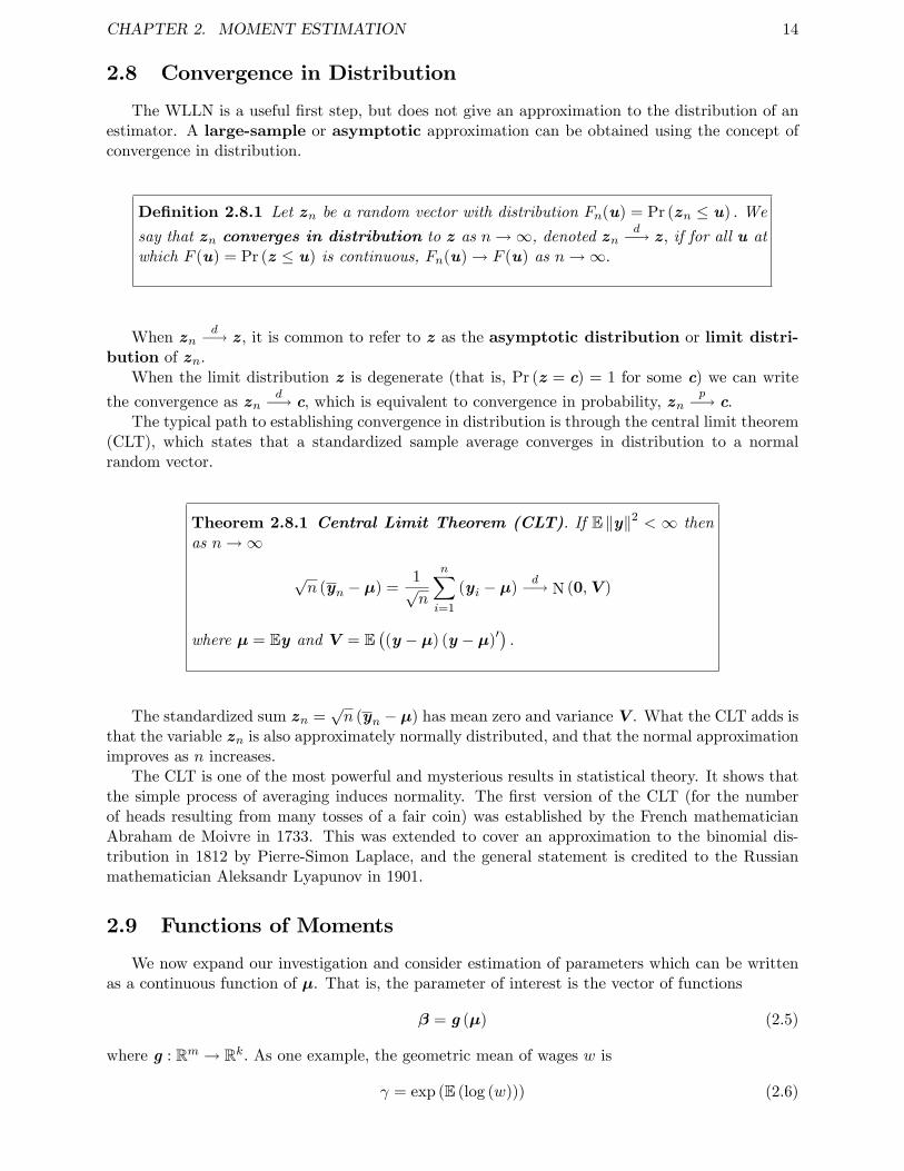
2.8 Convergence in Distribution
The WLLN is a useful first step, but does not give an approximation to the distribution of anestimator. A large-sample or asymptotic approximation can be obtained using the concept ofconvergence in distribution.
Definition 2.8.1 Let zn be a random vector with distribution Fn(u) = Pr (zn ≤ u) . We
say that zn converges in distribution to z as n→∞, denoted znd−→ z, if for all u at
which F (u) = Pr (z ≤ u) is continuous, Fn(u)→ F (u) as n→∞.
When znd−→ z, it is common to refer to z as the asymptotic distribution or limit distri-
bution of zn.When the limit distribution z is degenerate (that is, Pr (z = c) = 1 for some c) we can write
the convergence as znd−→ c, which is equivalent to convergence in probability, zn
p−→ c.The typical path to establishing convergence in distribution is through the central limit theorem
(CLT), which states that a standardized sample average converges in distribution to a normalrandom vector.
Theorem 2.8.1 Central Limit Theorem (CLT). If E ‖y‖2 < ∞ thenas n→∞
√n (yn − µ) =
1√n
n∑i=1
(yi − µ)d−→ N (0,V )
where µ = Ey and V = E((y − µ) (y − µ)′
).
The standardized sum zn =√n (yn − µ) has mean zero and variance V . What the CLT adds is
that the variable zn is also approximately normally distributed, and that the normal approximationimproves as n increases.
The CLT is one of the most powerful and mysterious results in statistical theory. It shows thatthe simple process of averaging induces normality. The first version of the CLT (for the numberof heads resulting from many tosses of a fair coin) was established by the French mathematicianAbraham de Moivre in 1733. This was extended to cover an approximation to the binomial dis-tribution in 1812 by Pierre-Simon Laplace, and the general statement is credited to the Russianmathematician Aleksandr Lyapunov in 1901.
2.9 Functions of Moments
We now expand our investigation and consider estimation of parameters which can be writtenas a continuous function of µ. That is, the parameter of interest is the vector of functions
β = g (µ) (2.5)
where g : Rm → Rk. As one example, the geometric mean of wages w is
γ = exp (E (log (w))) (2.6)
CHAPTER 2. MOMENT ESTIMATION 15
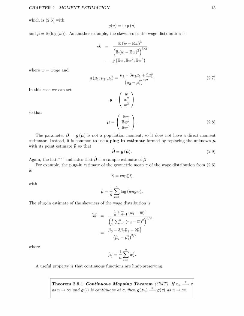
which is (2.5) withg(u) = exp (u)
and µ = E (log (w)) . As another example, the skewness of the wage distribution is
sk =E (w − Ew)3(E (w − Ew)2
)3/2
= g(Ew,Ew2,Ew3
)where w = wage and
g (µ1, µ2, µ3) =µ3 − 3µ2µ1 + 2µ3
1(µ2 − µ2
1
)3/2 . (2.7)
In this case we can set
y =
ww2
w3
so that
µ =
EwEw2
Ew3
. (2.8)
The parameter β = g (µ) is not a population moment, so it does not have a direct momentestimator. Instead, it is common to use a plug-in estimate formed by replacing the unknown µwith its point estimate µ so that
β = g (µ) . (2.9)
Again, the hat “^”indicates that β is a sample estimate of β.For example, the plug-in estimate of the geometric mean γ of the wage distribution from (2.6)
isγ = exp(µ)
with
µ =1
n
n∑i=1
log (wagei) .
The plug-in estimate of the skewness of the wage distribution is
sk =1n
∑ni=1 (wi − w)3(
1n
∑ni=1 (wi − w)2
)3/2
=µ3 − 3µ2µ1 + 2µ3
1(µ2 − µ2
1
)3/2where
µj =1
n
n∑i=1
wji .
A useful property is that continuous functions are limit-preserving.
Theorem 2.9.1 Continuous Mapping Theorem (CMT). If znp−→ c
as n→∞ and g (·) is continuous at c, then g(zn)p−→ g(c) as n→∞.
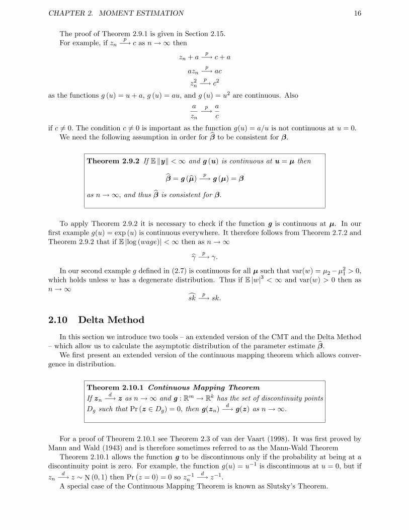
CHAPTER 2. MOMENT ESTIMATION 16
The proof of Theorem 2.9.1 is given in Section 2.15.For example, if zn
p−→ c as n→∞ then
zn + ap−→ c+ a
aznp−→ ac
z2n
p−→ c2
as the functions g (u) = u+ a, g (u) = au, and g (u) = u2 are continuous. Also
a
zn
p−→ a
c
if c 6= 0. The condition c 6= 0 is important as the function g(u) = a/u is not continuous at u = 0.We need the following assumption in order for β to be consistent for β.
Theorem 2.9.2 If E ‖y‖ <∞ and g (u) is continuous at u = µ then
β = g (µ)p−→ g (µ) = β
as n→∞, and thus β is consistent for β.
To apply Theorem 2.9.2 it is necessary to check if the function g is continuous at µ. In ourfirst example g(u) = exp (u) is continuous everywhere. It therefore follows from Theorem 2.7.2 andTheorem 2.9.2 that if E |log (wage)| <∞ then as n→∞
γp−→ γ.
In our second example g defined in (2.7) is continuous for all µ such that var(w) = µ2−µ21 > 0,
which holds unless w has a degenerate distribution. Thus if E |w|3 < ∞ and var(w) > 0 then asn→∞
skp−→ sk.
2.10 Delta Method
In this section we introduce two tools —an extended version of the CMT and the Delta Method—which allow us to calculate the asymptotic distribution of the parameter estimate β.
We first present an extended version of the continuous mapping theorem which allows conver-gence in distribution.
Theorem 2.10.1 Continuous Mapping TheoremIf zn
d−→ z as n→∞ and g : Rm → Rk has the set of discontinuity pointsDg such that Pr (z ∈ Dg) = 0, then g(zn)
d−→ g(z) as n→∞.
For a proof of Theorem 2.10.1 see Theorem 2.3 of van der Vaart (1998). It was first proved byMann and Wald (1943) and is therefore sometimes referred to as the Mann-Wald Theorem
Theorem 2.10.1 allows the function g to be discontinuous only if the probability at being at adiscontinuity point is zero. For example, the function g(u) = u−1 is discontinuous at u = 0, but if
znd−→ z ∼ N (0, 1) then Pr (z = 0) = 0 so z−1
nd−→ z−1.
A special case of the Continuous Mapping Theorem is known as Slutsky’s Theorem.
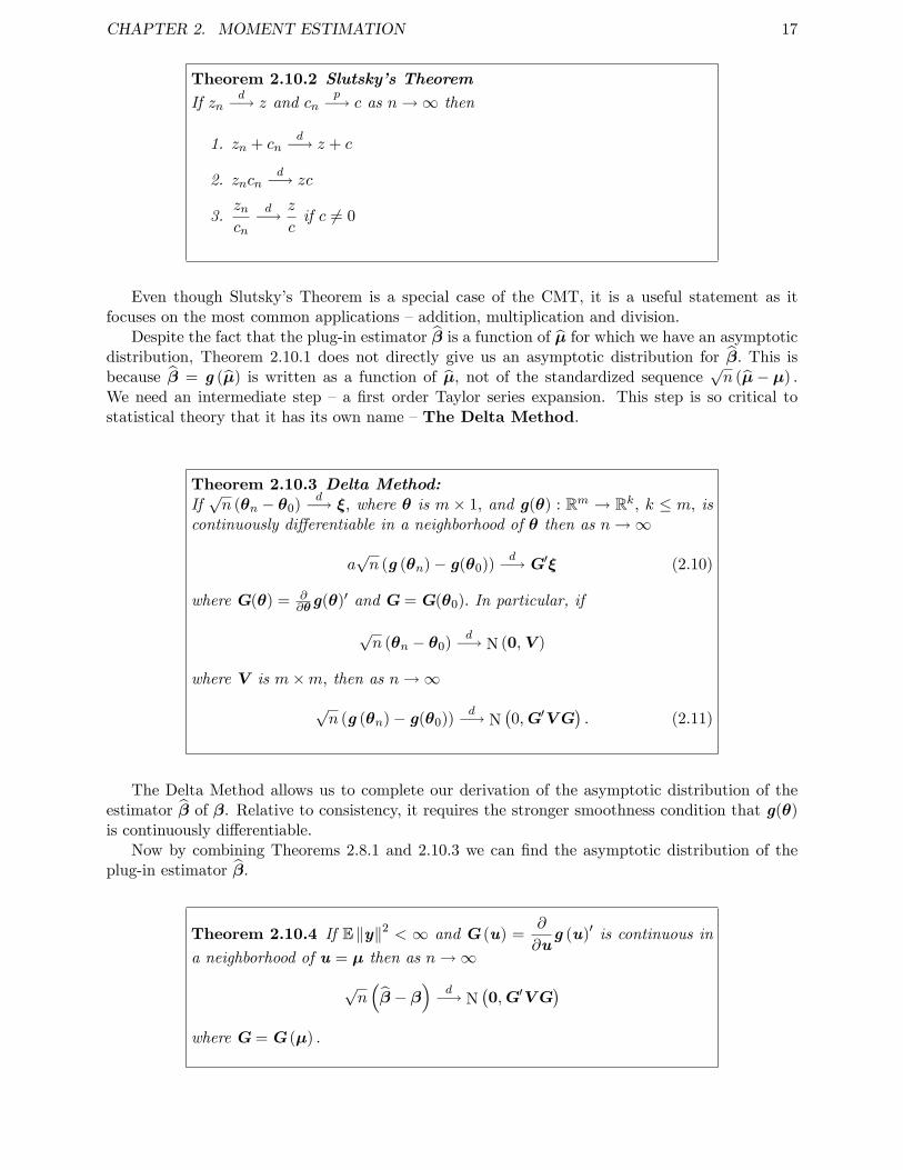
CHAPTER 2. MOMENT ESTIMATION 17
Theorem 2.10.2 Slutsky’s TheoremIf zn
d−→ z and cnp−→ c as n→∞ then
1. zn + cnd−→ z + c
2. zncnd−→ zc
3.zncn
d−→ z
cif c 6= 0
Even though Slutsky’s Theorem is a special case of the CMT, it is a useful statement as itfocuses on the most common applications —addition, multiplication and division.
Despite the fact that the plug-in estimator β is a function of µ for which we have an asymptoticdistribution, Theorem 2.10.1 does not directly give us an asymptotic distribution for β. This isbecause β = g (µ) is written as a function of µ, not of the standardized sequence
√n (µ− µ) .
We need an intermediate step —a first order Taylor series expansion. This step is so critical tostatistical theory that it has its own name —The Delta Method.
Theorem 2.10.3 Delta Method:If√n (θn − θ0)
d−→ ξ, where θ is m × 1, and g(θ) : Rm → Rk, k ≤ m, iscontinuously differentiable in a neighborhood of θ then as n→∞
a√n (g (θn)− g(θ0))
d−→ G′ξ (2.10)
where G(θ) = ∂∂θg(θ)′ and G = G(θ0). In particular, if
√n (θn − θ0)
d−→ N (0,V )
where V is m×m, then as n→∞√n (g (θn)− g(θ0))
d−→ N(0,G′V G
). (2.11)
The Delta Method allows us to complete our derivation of the asymptotic distribution of theestimator β of β. Relative to consistency, it requires the stronger smoothness condition that g(θ)is continuously differentiable.
Now by combining Theorems 2.8.1 and 2.10.3 we can find the asymptotic distribution of theplug-in estimator β.
Theorem 2.10.4 If E ‖y‖2 < ∞ and G (u) =∂
∂ug (u)′ is continuous in
a neighborhood of u = µ then as n→∞√n(β − β
)d−→ N
(0,G′V G
)where G = G (µ) .
CHAPTER 2. MOMENT ESTIMATION 18
2.11 Stochastic Order Symbols
It is convenient to have simple symbols for random variables and vectors which converge inprobability to zero or are stochastically bounded. The notation zn = op(1) (pronounced “smalloh-P-one”) means that zn
p−→ 0 as n→∞. We also say that
zn = op(an)
if an is a sequence such that a−1n zn = op(1). For example, for any consistent estimator β for β we
then can writeβ = β + op(1)
Similarly, the notation zn = Op(1) (pronounced “big on-P-one”) means that zn is bounded inprobability. Precisely, for any ε > 0 there is a constant Mε <∞ such that
limn→∞
Pr (|zn| > Mε) ≤ ε.
We say thatzn = Op(an)
if an is a sequence such that a−1n zn = Op(1).
Op(1) is weaker than op(1) in the sense that zn = op(1) implies zn = Op(1) but not the reverse.However, if zn = Op(an) then zn = op(bn) for any bn such that an/bn → 0.
If a random vector converges in distribution znd−→ z (for example, if z ∼ N (0,V )) then
zn = Op(1). It follows that for estimators β which satisfy the convergence of Theorem 2.10.4 thenwe can write
β = β +Op(n−1/2).
There are many simple rules for manipulating op(1) and Op(1) sequences which can be deducedfrom the continuous mapping theorem or Slutsky’s Theorem. For example,
op(1) + op(1) = op(1)
op(1) +Op(1) = Op(1)
Op(1) +Op(1) = Op(1)
op(1)op(1) = op(1)
op(1)Op(1) = op(1)
Op(1)Op(1) = Op(1)
2.12 Uniform Stochastic Bounds*
For some applications it can be useful to obtain the stochastic order of the random variable
max1≤i≤n
|yi| .
This is the magnitude of the largest observation in the sample y1, ..., yn. If the support of thedistribution of yi is unbounded, then as the sample size n increases, the largest observation willalso tend to increase. It turns out that there is a simple characterization.
Theorem 2.12.1 If E |y|r <∞ then as n→∞
n−1/r max1≤i≤n
|yi|p−→ 0
CHAPTER 2. MOMENT ESTIMATION 19
Equivalently,max
1≤i≤n|yi| = op(n
1/r). (2.12)
Theorem 2.12.1 says that the largest observation will diverge at a rate slower than n1/r. As rincreases this rate decreases. Thus the higher the moment, the slower the rate of divergence of thelargest observation.
To simplify the notation, we write (2.12) as
yi = op(n1/r)
uniformly in 1 ≤ i ≤ n. It is important to understand when the Op or op symbols are applied tosubscript i random variables we typically mean uniform convergence in the sense of (2.12).
Theorem 2.12.1 applies to random vectors. If E ‖y‖r <∞ then
max1≤i≤n
‖yi‖ = op(n1/r).
We now prove Theorem 2.12.1. Take any δ. The event
max1≤i≤n |yi| > δn1/rmeans that at
least one of the |yi| exceeds δn1/r, which is the same as the event⋃ni=1
|yi| > δn1/r
or equivalently⋃n
i=1 |yi|r > δrn . Since the probability of the union of events is smaller than the sum of the
probabilities,
Pr
(n−1/r max
1≤i≤n|yi| > δ
)= Pr
(n⋃i=1
|yi|r > δrn)
≤n∑i=1
Pr (|yi|r > nδr)
≤ 1
nδr
n∑i=1
E (|yi|r 1 (|yi|r > nδr))
=1
δrE (|yi|r 1 (|yi|r > nδr))
where the second inequality is the strong form of Markov’s inequality (Theorem B.25) and the finalequality is since the yi are iid. Since E |y|r <∞ this final expectation converges to zero as n→∞.This is because
E |yi|r =
∫|y|r dF (y) <∞
implies
E (|yi|r 1 (|yi|r > c)) =
∫|y|r>c
|y|r dF (y)→ 0
as c→∞. We have established that n−1/r max1≤i≤n |yi|p−→ 0, as required.
2.13 Semiparametric Effi ciency
In this section we argue that the sample mean µ and plug-in estimator β = g (µ) are effi cientestimators of the parameters µ and β. Our demonstration is based on the rich but technicallychallenging theory of semiparametric effi ciency bounds. An excellent accessible review has beenprovided by Newey (1990). We will also appeal to the asymptotic theory of maximum likelihoodestimation (see Section B.11).
We start by examining the sample mean µ, for the asymptotic effi ciency of β will follow fromthat of µ.
CHAPTER 2. MOMENT ESTIMATION 20
Recall, we know that if E ‖y‖2 < ∞ then the sample mean has the asymptotic distribution√n (µ− µ)
d−→ N (0,V ) .We want to know if µ is the best feasible estimator, or if there is anotherestimator with a smaller asymptotic variance. While it seems intuitively unlikely that anotherestimator could have a smaller asymptotic variance, how do we know that this is not the case?
When we ask if µ is the best estimator, we need to be clear about the class of models —the classof permissible distributions. For estimation of the mean µ of the distribution of y the broadestconceivable class is L1 = F : E ‖y‖ <∞ . This class is too broad n for our current purposes, asµ is not asymptotically N (0,V ) for all F ∈ L1. A more realistic choice is L2 =
F : E ‖y‖2 <∞
—the class of finite-variance distributions. When we seek an effi cient estimator of the mean µ inthe class of models L2 what we are seeking is the best estimator, given that all we know is thatF ∈ L2.
To show that the answer is not immediately obvious, it might be helpful to review a set-ting where the sample mean is ineffi cient. Suppose that y ∈ R has the double exponential den-sity f (y | µ) = 2−1/2 exp
(− |y − µ|
√2). Since var (y) = 1 we see that the sample mean sat-
isfies√n (µ− µ)
d−→ N (0, 1). In this model the maximum likelihood estimator (MLE) µ forµ is the sample median. Recall from the theory of maximum likelhood that the MLE satisfies√n (µ− µ)
d−→ N(
0,(ES2
)−1)where S = ∂
∂µ log f (y | µ) = −√
2 sgn (y − µ) is the score. We can
calculate that ES2 = 2 and thus conclude that√n (µ− µ)
d−→ N (0, 1/2) . The asymptotic varianceof the MLE is one-half that of the sample mean. Thus when the true density is known to be doubleexponential the sample mean is ineffi cient.
But the estimator which achieves this improved effi ciency —the sample median —is not generi-cally consistent for the population mean. It is inconsistent if the density is asymmetric or skewed.So the improvement comes at a great cost. Another way of looking at this is that the samplemedian is effi cient in the class of densities
f (y | µ) = 2−1/2 exp
(− |y − µ|
√2)but unless it is
known that this is the correct distribution class this knowledge is not very useful.The relevant question is whether or not the sample mean is effi cient when the form of the
distribution is unknown. We call this setting semiparametric as the parameter of interest (themean) is finite dimensional while the remaining features of the distribution are unspecified. In thesemiparametric context an estimator is called semiparametrically effi cient if it has the smallestasymptotic variance among all semiparametric estimators.
The mathematical trick is to reduce the semiparametric model to a set of parametric “submod-els”. The Cramer-Rao variance bound can be found for each parametric submodel. The variancebound for the semiparametric model (the union of the submodels) is then defined as the supremumof the individual variance bounds.
Formally, suppose that the true density of y is the unknown function f(y) with mean µ = Ey =∫yf(y)dy. A parametric submodel η for f(y) is a density fη (y | θ) which is a smooth function of
a parameter θ, and there is a true value θ0 such that fη (y | θ0) = f(y). The index η indicates thesubmodels. The equality fη (y | θ0) = f(y) means that the submodel class passes through the truedensity, so the submodel is a true model. The class of submodels η and parameter θ0 depend onthe true density f. In the submodel fη (y | θ) , the mean is µη(θ) =
∫yfη (y | θ) dy which varies
with the parameter θ. Let η ∈ ℵ be the class of all submodels for f.Since each submodel η is parametric we can calculate the effi ciency bound for estimation of µ
within this submodel. Specifically, given the density fη (y | θ) its likelihood score is
Sη =∂
∂θlog fη (y | θ0) ,
so the Cramer-Rao lower bound for estimation of θ is(ESηS′η
)−1. Defining Mη = ∂
∂θµη(θ0)′,
by Theorem B.11.5 the Cramer-Rao lower bound for estimation of µ within the submodel η is
V η = M ′η
(ESηS′η
)−1Mη.
CHAPTER 2. MOMENT ESTIMATION 21
As V η is the effi ciency bound for the submodel class fη (y | θ) , no estimator can have anasymptotic variance smaller than V η for any density fη (y | θ) in the submodel class, including thetrue density f . This is true for all submodels η. Thus the asymptotic variance of any semiparametricestimator cannot be smaller than V η for any conceivable submodel. Taking the supremum of theCramer-Rao bounds lower from all conceivable submodels we define2
V = supη∈ℵ
V η.
The asymptotic variance of any semiparametric estimator cannot be smaller than V , since it cannotbe smaller than any individual V η.We call V the semiparametric asymptotic variance boundor semiparametric effi ciency bound for estimation of µ, as it is a lower bound on the asymptoticvariance for any semiparametric estimator. If the asymptotic variance of a specific semiparametricestimator equals the bound V we say that the estimator is semiparametrically effi cient.
For many statistical problems it is quite challenging to calculate the semiparametric variancebound. However, in some cases there is a simple method to find the solution. Suppose thatwe can find a submodel η0 whose Cramer-Rao lower bound satisfies V η0 = V µ where V µ isthe asymptotic variance of a known semiparametric estimator. In this case, we can deduce thatV = V η0 = V µ. Otherwise there would exist another submodel η1 whose Cramer-Rao lower boundsatisfies V η0 < V η1 but this would imply V µ < V η1 which contradicts the Cramer-Rao Theorem.
We now find this submodel for the sample mean µ. Our goal is to find a parametric submodelwhose Cramer-Rao bound for µ is V . This can be done by creating a tilted version of the truedensity. Consider the parametric submodel
fη (y | θ) = f(y)(1 + θ′V −1 (y − µ)
)(2.13)
where f(y) is the true density and µ = Ey. Note that∫fη (y | θ) dy =
∫f(y)dy + θ′V −1
∫f(y) (y − µ) dy = 1
and for all θ close to zero fη (y | θ) ≥ 0. Thus fη (y | θ) is a valid density function. It is a parametricsubmodel since fη (y | θ0) = f(y) when θ0 = 0. This parametric submodel has the mean
µ(θ) =
∫yfη (y | θ) dy
=
∫yf(y)dy +
∫f(y)y (y − µ)′ V −1θdy
= µ+ θ
which is a smooth function of θ.Since
∂
∂θlog fη (y | θ) =
∂
∂θlog(1 + θ′V −1 (y − µ)
)=
V −1 (y − µ)
1 + θ′V −1 (y − µ)
it follows that the score function for θ is
Sη =∂
∂θlog fη (y | θ0) = V −1 (y − µ) . (2.14)
By Theorem B.11.3 the Cramer-Rao lower bound for θ is(E(SηS
′η
))−1=(V −1E
((y − µ) (y − µ)′
)V −1
)−1= V . (2.15)
2 It is not obvious that this supremum exists, as V η is a matrix so there is not a unique ordering of matrices.However, in many cases (including the ones we study) the supremum exists and is unique.
CHAPTER 2. MOMENT ESTIMATION 22
The Cramer-Rao lower bound for µ(θ) = µ+ θ is also V , and this equals the asymptotic varianceof the moment estimator µ. This was what we set out to show.
In summary, we have shown that in the submodel (2.13) the Cramer-Rao lower bound forestimation of µ is V which equals the asymptotic variance of the sample mean. This establishesthe following result.
Proposition 2.13.1 In the class of distributions F ∈ L2, the semipara-metric variance bound for estimation of µ is V = var(yi), and the samplemean µ is a semiparametrically effi cient estimator of the population meanµ.
We call this result a proposition rather than a theorem as we have not attended to the regularityconditions.
It is a simple matter to extend this result to the plug-in estimator β = g (µ). We know fromTheorem 2.10.4 that if E ‖y‖2 <∞ and g (u) is continuously differentiable at u = µ then the plug-in
estimator has the asymptotic distribution√n(β − β
)d−→ N (0,G′V G) .We therefore consider the
class of distributions L2(g) =F : E ‖y‖2 <∞, g (u) is continuously differentiable at u = Ey
.
For example, if β = µ1/µ2 where µ1 = Ey1 and µ2 = Ey2 then L2(g) =F : Ey2
1 <∞, Ey22 <∞, and Ey2 6= 0
.
For any submodel η the Cramer-Rao lower bound for estimation of β = g (µ) is G′V ηG byTheorem B.11.5. For the submodel (2.13) this bound isG′V G which equals the asymptotic varianceof β from Theorem 2.10.4. Thus β is semiparametrically effi cient.
Proposition 2.13.2 In the class of distributions F ∈ L2(g) the semipara-metric variance bound for estimation of β = g (µ) is G′V G, and the plug-inestimator β = g (µ) is a semiparametrically effi cient estimator of β.
The result in Proposition 2.13.2 is quite general. Smooth functions of sample moments areeffi cient estimators for their population counterparts. This is a very powerful result, as mosteconometric estimators can be written (or approximated) as smooth functions of sample means.
2.14 Expectation*
For any random variable y we define the mean or expectation Ey as follows. If y is discrete,
Ey =∞∑j=1
τ j Pr (y = τ j) ,
and if y is continuous with density f
Ey =
∫ ∞−∞
yf(y)dy.
We can unify these definitions by writing the expectation as the Lebesgue integral with respect tothe distribution function F
Ey =
∫ ∞−∞
ydF (y).
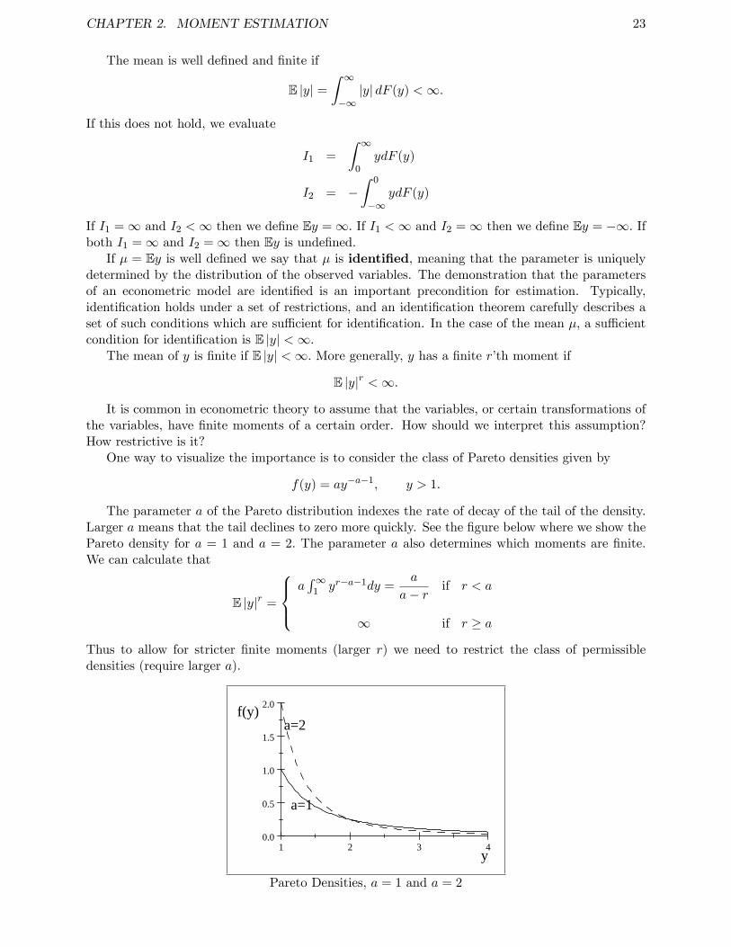
CHAPTER 2. MOMENT ESTIMATION 23
The mean is well defined and finite if
E |y| =∫ ∞−∞|y| dF (y) <∞.
If this does not hold, we evaluate
I1 =
∫ ∞0
ydF (y)
I2 = −∫ 0
−∞ydF (y)
If I1 =∞ and I2 <∞ then we define Ey =∞. If I1 <∞ and I2 =∞ then we define Ey = −∞. Ifboth I1 =∞ and I2 =∞ then Ey is undefined.
If µ = Ey is well defined we say that µ is identified, meaning that the parameter is uniquelydetermined by the distribution of the observed variables. The demonstration that the parametersof an econometric model are identified is an important precondition for estimation. Typically,identification holds under a set of restrictions, and an identification theorem carefully describes aset of such conditions which are suffi cient for identification. In the case of the mean µ, a suffi cientcondition for identification is E |y| <∞.
The mean of y is finite if E |y| <∞. More generally, y has a finite r’th moment if
E |y|r <∞.
It is common in econometric theory to assume that the variables, or certain transformations ofthe variables, have finite moments of a certain order. How should we interpret this assumption?How restrictive is it?
One way to visualize the importance is to consider the class of Pareto densities given by
f(y) = ay−a−1, y > 1.
The parameter a of the Pareto distribution indexes the rate of decay of the tail of the density.Larger a means that the tail declines to zero more quickly. See the figure below where we show thePareto density for a = 1 and a = 2. The parameter a also determines which moments are finite.We can calculate that
E |y|r =
a∫∞
1 yr−a−1dy =a
a− r if r < a
∞ if r ≥ a
Thus to allow for stricter finite moments (larger r) we need to restrict the class of permissibledensities (require larger a).
1 2 3 40.0
0.5
1.0
1.5
2.0
y
f(y)a=2
a=1
Pareto Densities, a = 1 and a = 2
CHAPTER 2. MOMENT ESTIMATION 24
Thus, broadly speaking, the restriction that y has a finite r’th moment means that the tail of y’sdensity declines to zero faster than y−r−1. The faster decline of the tail means that the probabilityof observing an extreme value of y is a more rare event.
It is helpful to know that the existence of finite moments is monotonic. Liapunov’s Inequality(B.23) implies that if E |y|p < ∞ for some p > 0, then E |y|r < ∞ for all 0 ≤ r ≤ p. For example,Ey2 <∞ implies E |y| <∞ and thus both the mean and variance of y are finite.
2.15 Technical Proofs*
In this section we provide proofs of some of the more technical points in the chapter. Theseproofs may only be of interest to more mathematically inclined.
Proof of Theorem 2.6.1: Without loss of generality, we can assume E(yi) = 0 by recentering yion its expectation.
We need to show that for all δ > 0 and η > 0 there is some N < ∞ so that for all n ≥ N,Pr (|y| > δ) ≤ η. Fix δ and η. Set ε = δη/3. Pick C <∞ large enough so that
E (|yi| 1 (|yi| > C)) ≤ ε (2.16)
(where 1 (·) is the indicator function) which is possible since E |yi| <∞. Define the random variables
wi = yi1 (|yi| ≤ C)− E (yi1 (|yi| ≤ C))
zi = yi1 (|yi| > C)− E (yi1 (|yi| > C))
so thaty = w + z
andE |y| ≤ E |w|+ E |z| . (2.17)
We now show that sum of the expectations on the right-hand-side can be bounded below 3ε.First, by the Triangle Inequality (A.9) and the Expectation Inequality (B.18),
E |zi| = E |yi1 (|yi| > C)− E (yi1 (|yi| > C))|≤ E |yi1 (|yi| > C)|+ |E (yi1 (|yi| > C))|≤ 2E |yi1 (|yi| > C)|≤ 2ε, (2.18)
and thus by the Triangle Inequality (A.9) and (2.18)
E |z| = E
∣∣∣∣∣ 1nn∑i=1
zi
∣∣∣∣∣ ≤ 1
n
n∑i=1
E |zi| ≤ 2ε. (2.19)
Second, by a similar argument
|wi| = |yi1 (|yi| ≤ C)− E (yi1 (|yi| ≤ C))|≤ |yi1 (|yi| ≤ C)|+ |E (yi1 (|yi| ≤ C))|≤ 2 |yi1 (|yi| ≤ C)|≤ 2C (2.20)
where the final inequality is (2.16). Then by Jensen’s Inequality (B.15), the fact that the wi areiid and mean zero, and (2.20),
(E |w|)2 ≤ E |w|2 =Ew2
i
n=
4C2
n≤ ε2 (2.21)
CHAPTER 2. MOMENT ESTIMATION 25
the final inequality holding for n ≥ 4C2/ε2 = 36C2/δ2η2. Equations (2.17), (2.19) and (2.21)together show that
E |y| ≤ 3ε2 (2.22)
as desired.Finally, by Markov’s Inequality (B.24) and (2.22),
Pr (|y| > δ) ≤ E |y|δ≤ 3ε
δ= η,
the final equality by the definition of ε. We have shown that for any δ > 0 and η > 0 then for alln ≥ 36C2/δ2η2, Pr (|y| > δ) ≤ η, as needed.
Proof of Theorem 2.7.1: By Loève’s cr Inequality (B.14)
‖y‖ =
m∑j=1
y2j
1/2
≤m∑j=1
|yj | .
Thus if E |yj | <∞ for j = 1, ...,m, then
E ‖y‖ ≤m∑j=1
E |yj | <∞.
For the reverse inequality, the Euclidean norm of a vector is larger than the length of any individualcomponent, so for any j, |yj | ≤ ‖y‖ . Thus, if E ‖y‖ <∞, then E |yj | <∞ for j = 1, ...,m.
Proof of Theorem 2.8.1: The moment bound Ey′iyi < ∞ is suffi cient to guarantee that theelements of µ and V are well defined and finite. Without loss of generality, it is suffi cient toconsider the case µ = 0.
Our proof method is to calculate the characteristic function of√nyn and show that it converges
pointwise to the characteristic function of N (0,V ) . By Lévy’s Continuity Theorem (see Van derVaart (2008) Theorem 2.13) this is suffi cient to established that
√nyn converges in distribution to
N (0,V ) .For λ ∈ Rm, let C (λ) = E exp
(iλ′yi
)denote the characteristic function of yi and set c (λ) =
logC(λ). Since yi has two finite moments the first and second derivatives of C(λ) are continuousin λ. They are
∂
∂λC(λ) = iE
(yi exp
(iλ′yi
))∂2
∂λ∂λ′C(λ) = i2E
(yiy
′i exp
(iλ′yi
)).
When evaluated at λ = 0
C(0) = 1
∂
∂λC(0) = iE (yi) = 0
∂2
∂λ∂λ′C(0) = −E
(yiy
′i
)= −V .
Furthermore,
cλ(λ) =∂
∂λc(λ) = C(λ)−1 ∂
∂λC(λ)
cλλ(λ) =∂2
∂λ∂λ′c(λ) = C(λ)−1 ∂2
∂λ∂λ′C(λ)− C(λ)−2 ∂
∂λC (λ)
∂
∂λ′C(λ)
CHAPTER 2. MOMENT ESTIMATION 26
so when evaluated at λ = 0
c(0) = 0
cλ(0) = 0
cλλ(0) = −V .
By a second-order Taylor series expansion of c(λ) about λ = 0,
c(λ) = c(0) + cλ(0)′λ+1
2λ′cλλ(λ∗)λ =
1
2λ′cλλ(λ∗)λ (2.23)
where λ∗ lies on the line segment joining 0 and λ.We now compute Cn(λ) = E exp
(iλ′√nyn
), the characteristic function of
√nyn. By the prop-
erties of the exponential function, the independence of the yi, the definition of c(λ) and (2.23)
logCn(λ) = logE exp
(i
1√n
n∑i=1
λ′yi
)
= logEn∏i=1
exp
(i
1√nλ′yi
)
= log
n∏i=1
E exp
(i
1√nλ′yi
)
=
n∑i=1
logE exp
(i
1√nλ′yi
)= nc
(λ√n
)=
1
2λ′cλλ(λn)λ
where λn lies on the line segment joining 0 and λ/√n. Since λn → 0 and cλλ(λ) is continuous,
cλλ(λn)→ cλλ(0) = −V. We thus find that as n→∞,
logCn(λ)→ −1
2λ′V λ
and
Cn(λ)→ exp
(−1
2λ′V λ
)which is the characteristic function of the N (0,V ) distribution. This completes the proof.
Proof of Theorem 2.9.1: Since g is continuous at c, for all ε > 0 we can find a δ > 0 suchthat if ‖zn − c‖ < δ then ‖g (zn)− g (c)‖ ≤ ε. Recall that A ⊂ B implies Pr(A) ≤ Pr(B). ThusPr (‖g (zn)− g (c)‖ ≤ ε) ≥ Pr (‖zn − c‖ < δ) → 1 as n → ∞ by the assumption that zn
p−→ c.
Hence g(zn)p−→ g(c) as n→∞.
Proof of Theorem 2.10.3: By a vector Taylor series expansion, for each element of g,
gj(θn) = gj(θ) + gjθ(θ∗jn) (θn − θ)
where θ∗nj lies on the line segment between θn and θ and therefore converges in probability to θ.
It follows that ajn = gjθ(θ∗jn)− gjθp−→ 0. Stacking across elements of g, we find
√n (g (θn)− g(θ)) = (G+ an)′
√n (θn − θ)
d−→ G′ξ. (2.24)
CHAPTER 2. MOMENT ESTIMATION 27
The convergence is by Theorem 2.10.1, as G+ and−→ G,
√n (θn − θ)
d−→ ξ, and their product iscontinuous. This establishes (2.10)
When ξ ∼ N (0,V ) , the right-hand-side of (2.24) equals
G′ξ = G′N (0,V ) = N(0,G′V G
)establishing (2.11).
Chapter 3
Conditional Expectation andProjection
3.1 Introduction
The most commonly applied econometric tool is least-squares estimation, also known as regres-sion. As we will see, least-squares is a tool to estimate an approximate conditional mean of onevariable (the dependent variable) given another set of variables (the regressors, conditioningvariables, or covariates).
In this chapter we abstract from estimation, and focus on the probabilistic foundation of theconditional expectation model and its projection approximation.
3.2 The Distribution of Wages
Suppose that we are interested in wage rates in the United States. Since wage rates vary acrossworkers, we cannot describe wage rates by a single number. Instead, we can describe wages using aprobability distribution. Formally, we view the wage of an individual worker as a random variablewage with the probability distribution
F (u) = Pr(wage ≤ u).
When we say that a person’s wage is random we mean that we do not know their wage before it ismeasured, and we treat observed wage rates as realizations from the distribution F. Treating un-observed wages as random variables and observed wages as realizations is a powerful mathematicalabstraction which allows us to use the tools of mathematical probability.
A useful thought experiment is to imagine dialing a telephone number selected at random, andthen asking the person who responds to tell us their wage rate. (Assume for simplicity that allworkers have equal access to telephones, and that the person who answers your call will respondhonestly.) In this thought experiment, the wage of the person you have called is a single draw fromthe distribution F of wages in the population. By making many such phone calls we can learn thedistribution F of the entire population.
When a distribution function F is differentiable we define the probability density function
f(u) =d
duF (u).
The density contains the same information as the distribution function, but the density is typicallyeasier to visually interpret.
28
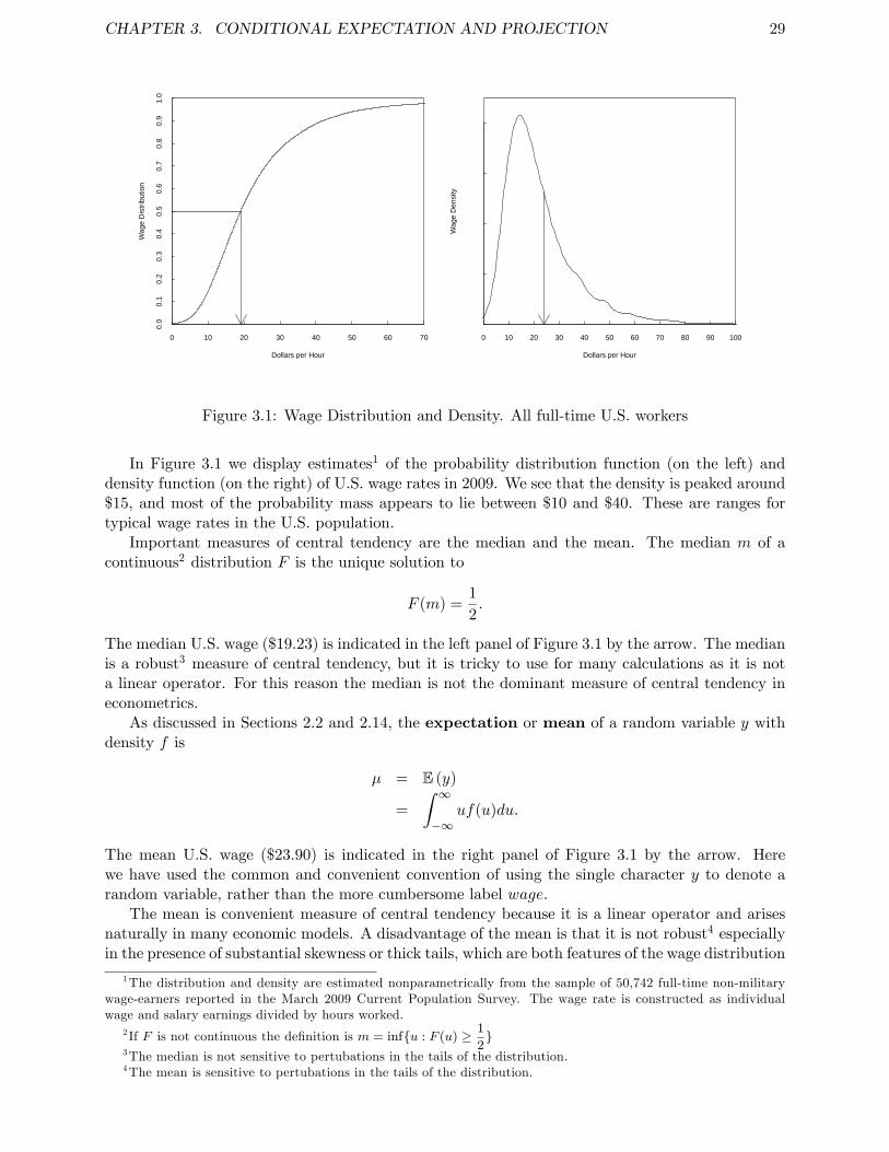
CHAPTER 3. CONDITIONAL EXPECTATION AND PROJECTION 29
Dollars per Hour
Wag
e D
istr
ibut
ion
0 10 20 30 40 50 60 70
0.0
0.1
0.2
0.3
0.4
0.5
0.6
0.7
0.8
0.9
1.0
Dollars per Hour
Wag
e D
ensi
ty
0 10 20 30 40 50 60 70 80 90 100
Figure 3.1: Wage Distribution and Density. All full-time U.S. workers
In Figure 3.1 we display estimates1 of the probability distribution function (on the left) anddensity function (on the right) of U.S. wage rates in 2009. We see that the density is peaked around$15, and most of the probability mass appears to lie between $10 and $40. These are ranges fortypical wage rates in the U.S. population.
Important measures of central tendency are the median and the mean. The median m of acontinuous2 distribution F is the unique solution to
F (m) =1
2.
The median U.S. wage ($19.23) is indicated in the left panel of Figure 3.1 by the arrow. The medianis a robust3 measure of central tendency, but it is tricky to use for many calculations as it is nota linear operator. For this reason the median is not the dominant measure of central tendency ineconometrics.
As discussed in Sections 2.2 and 2.14, the expectation or mean of a random variable y withdensity f is
µ = E (y)
=
∫ ∞−∞
uf(u)du.
The mean U.S. wage ($23.90) is indicated in the right panel of Figure 3.1 by the arrow. Herewe have used the common and convenient convention of using the single character y to denote arandom variable, rather than the more cumbersome label wage.
The mean is convenient measure of central tendency because it is a linear operator and arisesnaturally in many economic models. A disadvantage of the mean is that it is not robust4 especiallyin the presence of substantial skewness or thick tails, which are both features of the wage distribution
1The distribution and density are estimated nonparametrically from the sample of 50,742 full-time non-militarywage-earners reported in the March 2009 Current Population Survey. The wage rate is constructed as individualwage and salary earnings divided by hours worked.
2 If F is not continuous the definition is m = infu : F (u) ≥ 1
2
3The median is not sensitive to pertubations in the tails of the distribution.4The mean is sensitive to pertubations in the tails of the distribution.
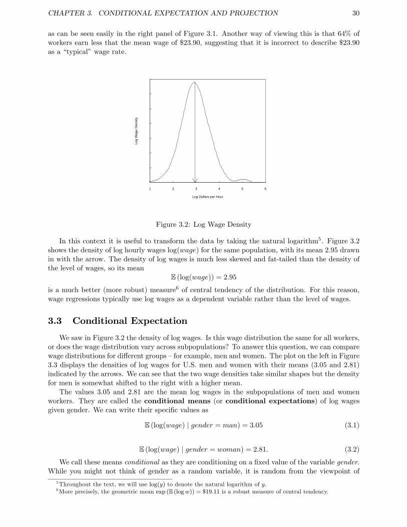
CHAPTER 3. CONDITIONAL EXPECTATION AND PROJECTION 30
as can be seen easily in the right panel of Figure 3.1. Another way of viewing this is that 64% ofworkers earn less that the mean wage of $23.90, suggesting that it is incorrect to describe $23.90as a “typical”wage rate.
Log Dollars per Hour
Log
Wag
e D
ensi
ty
1 2 3 4 5 6
Figure 3.2: Log Wage Density
In this context it is useful to transform the data by taking the natural logarithm5. Figure 3.2shows the density of log hourly wages log(wage) for the same population, with its mean 2.95 drawnin with the arrow. The density of log wages is much less skewed and fat-tailed than the density ofthe level of wages, so its mean
E (log(wage)) = 2.95
is a much better (more robust) measure6 of central tendency of the distribution. For this reason,wage regressions typically use log wages as a dependent variable rather than the level of wages.
3.3 Conditional Expectation
We saw in Figure 3.2 the density of log wages. Is this wage distribution the same for all workers,or does the wage distribution vary across subpopulations? To answer this question, we can comparewage distributions for different groups —for example, men and women. The plot on the left in Figure3.3 displays the densities of log wages for U.S. men and women with their means (3.05 and 2.81)indicated by the arrows. We can see that the two wage densities take similar shapes but the densityfor men is somewhat shifted to the right with a higher mean.
The values 3.05 and 2.81 are the mean log wages in the subpopulations of men and womenworkers. They are called the conditional means (or conditional expectations) of log wagesgiven gender. We can write their specific values as
E (log(wage) | gender = man) = 3.05 (3.1)
E (log(wage) | gender = woman) = 2.81. (3.2)
We call these means conditional as they are conditioning on a fixed value of the variable gender.While you might not think of gender as a random variable, it is random from the viewpoint of
5Throughout the text, we will use log(y) to denote the natural logarithm of y.6More precisely, the geometric mean exp (E (logw)) = $19.11 is a robust measure of central tendency.
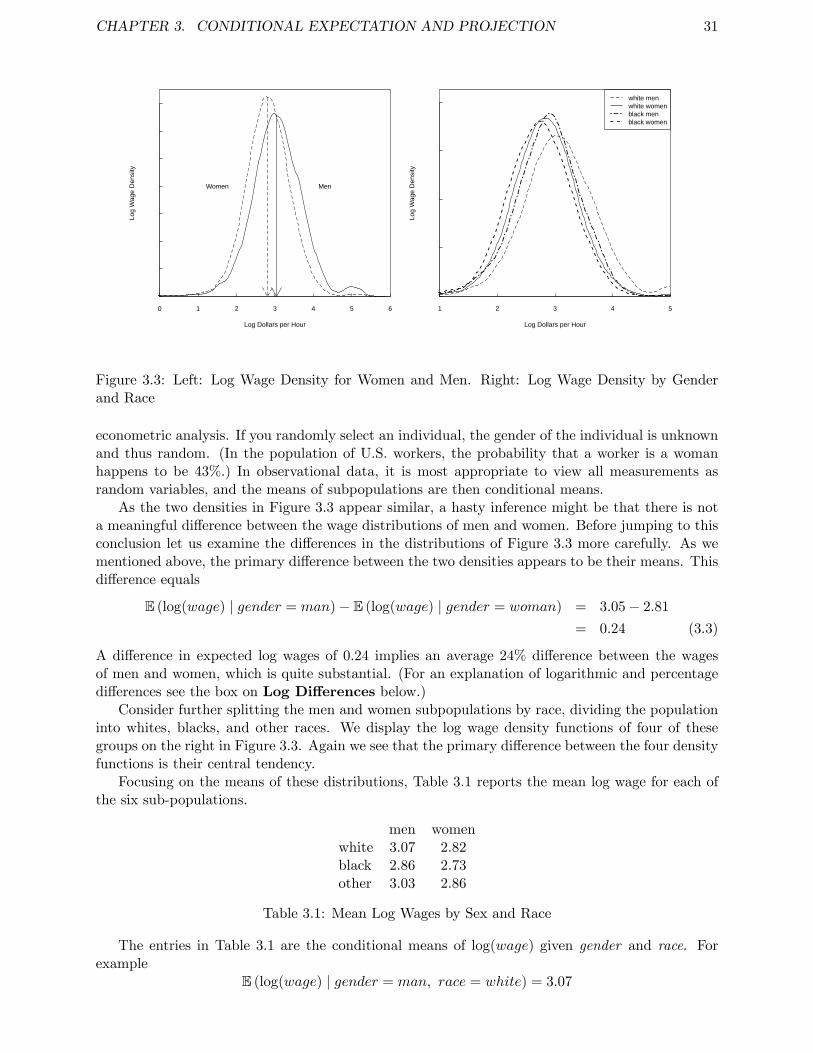
CHAPTER 3. CONDITIONAL EXPECTATION AND PROJECTION 31
Log Dollars per Hour
Log
Wag
e D
ensi
ty
0 1 2 3 4 5 6
MenWomen
Log Dollars per Hour
Log
Wag
e D
ensi
ty
1 2 3 4 5
white menwhite womenblack menblack women
Figure 3.3: Left: Log Wage Density for Women and Men. Right: Log Wage Density by Genderand Race
econometric analysis. If you randomly select an individual, the gender of the individual is unknownand thus random. (In the population of U.S. workers, the probability that a worker is a womanhappens to be 43%.) In observational data, it is most appropriate to view all measurements asrandom variables, and the means of subpopulations are then conditional means.
As the two densities in Figure 3.3 appear similar, a hasty inference might be that there is nota meaningful difference between the wage distributions of men and women. Before jumping to thisconclusion let us examine the differences in the distributions of Figure 3.3 more carefully. As wementioned above, the primary difference between the two densities appears to be their means. Thisdifference equals
E (log(wage) | gender = man)− E (log(wage) | gender = woman) = 3.05− 2.81
= 0.24 (3.3)
A difference in expected log wages of 0.24 implies an average 24% difference between the wagesof men and women, which is quite substantial. (For an explanation of logarithmic and percentagedifferences see the box on Log Differences below.)
Consider further splitting the men and women subpopulations by race, dividing the populationinto whites, blacks, and other races. We display the log wage density functions of four of thesegroups on the right in Figure 3.3. Again we see that the primary difference between the four densityfunctions is their central tendency.
Focusing on the means of these distributions, Table 3.1 reports the mean log wage for each ofthe six sub-populations.
men womenwhite 3.07 2.82black 2.86 2.73other 3.03 2.86
Table 3.1: Mean Log Wages by Sex and Race
The entries in Table 3.1 are the conditional means of log(wage) given gender and race. Forexample
E (log(wage) | gender = man, race = white) = 3.07

CHAPTER 3. CONDITIONAL EXPECTATION AND PROJECTION 32
andE (log(wage) | gender = woman, race = black) = 2.73
One benefit of focusing on conditional means is that they reduce complicated distributionsto a single summary measure, and thereby facilitate comparisons across groups. Because of thissimplifying property, conditional means are the primary interest of regression analysis and are amajor focus in econometrics.
Table 3.1 allows us to easily calculate average wage differences between groups. For example,we can see that the wage gap between men and women continues after disaggregation by race, asthe average gap between white men and white women is 25%, and that between black men andblack women is 13%. We also can see that there is a race gap, as the average wages of blacks aresubstantially less than the other race categories. In particular, the average wage gap between whitemen and black men is 21%, and that between white women and black women is 9%.
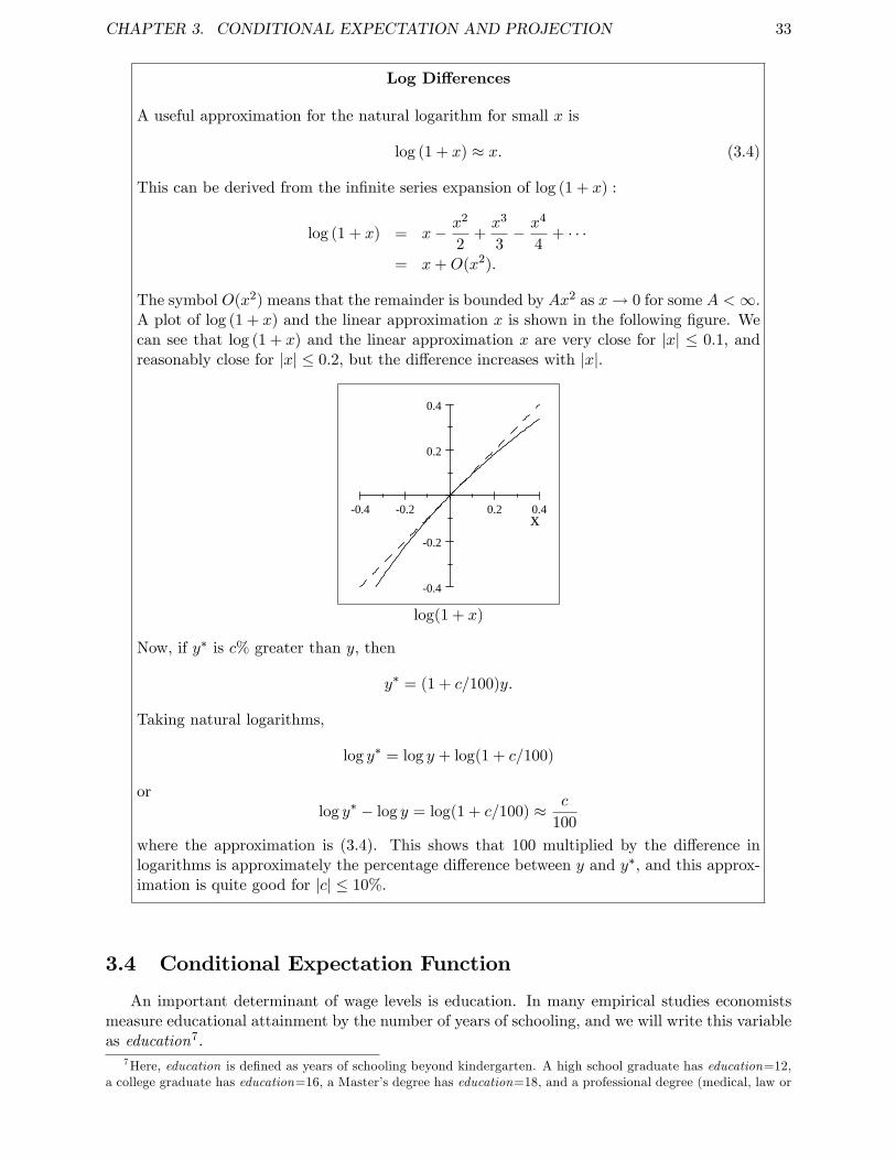
CHAPTER 3. CONDITIONAL EXPECTATION AND PROJECTION 33
Log Differences
A useful approximation for the natural logarithm for small x is
log (1 + x) ≈ x. (3.4)
This can be derived from the infinite series expansion of log (1 + x) :
log (1 + x) = x− x2
2+x3
3− x4
4+ · · ·
= x+O(x2).
The symbol O(x2) means that the remainder is bounded by Ax2 as x→ 0 for some A <∞.A plot of log (1 + x) and the linear approximation x is shown in the following figure. Wecan see that log (1 + x) and the linear approximation x are very close for |x| ≤ 0.1, andreasonably close for |x| ≤ 0.2, but the difference increases with |x|.
0.4 0.2 0.2 0.4
0.4
0.2
0.2
0.4
x
log(1 + x)
Now, if y∗ is c% greater than y, then
y∗ = (1 + c/100)y.
Taking natural logarithms,
log y∗ = log y + log(1 + c/100)
orlog y∗ − log y = log(1 + c/100) ≈ c
100
where the approximation is (3.4). This shows that 100 multiplied by the difference inlogarithms is approximately the percentage difference between y and y∗, and this approx-imation is quite good for |c| ≤ 10%.
3.4 Conditional Expectation Function
An important determinant of wage levels is education. In many empirical studies economistsmeasure educational attainment by the number of years of schooling, and we will write this variableas education7.
7Here, education is defined as years of schooling beyond kindergarten. A high school graduate has education=12,a college graduate has education=16, a Master’s degree has education=18, and a professional degree (medical, law or
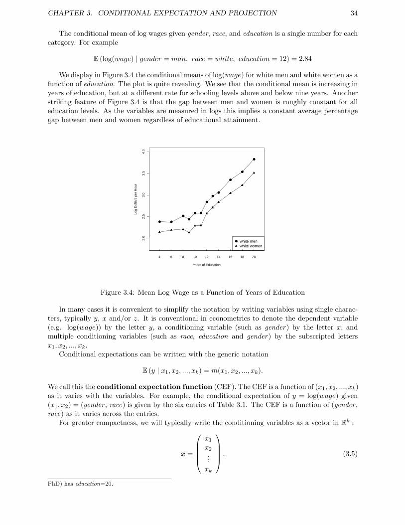
CHAPTER 3. CONDITIONAL EXPECTATION AND PROJECTION 34
The conditional mean of log wages given gender, race, and education is a single number for eachcategory. For example
E (log(wage) | gender = man, race = white, education = 12) = 2.84
We display in Figure 3.4 the conditional means of log(wage) for white men and white women as afunction of education. The plot is quite revealing. We see that the conditional mean is increasing inyears of education, but at a different rate for schooling levels above and below nine years. Anotherstriking feature of Figure 3.4 is that the gap between men and women is roughly constant for alleducation levels. As the variables are measured in logs this implies a constant average percentagegap between men and women regardless of educational attainment.
2.0
2.5
3.0
3.5
4.0
Years of Education
Log
Dol
lars
per
Hou
r
4 6 8 10 12 14 16 18 20
white menwhite women
Figure 3.4: Mean Log Wage as a Function of Years of Education
In many cases it is convenient to simplify the notation by writing variables using single charac-ters, typically y, x and/or z. It is conventional in econometrics to denote the dependent variable(e.g. log(wage)) by the letter y, a conditioning variable (such as gender) by the letter x, andmultiple conditioning variables (such as race, education and gender) by the subscripted lettersx1, x2, ..., xk.
Conditional expectations can be written with the generic notation
E (y | x1, x2, ..., xk) = m(x1, x2, ..., xk).
We call this the conditional expectation function (CEF). The CEF is a function of (x1, x2, ..., xk)as it varies with the variables. For example, the conditional expectation of y = log(wage) given(x1, x2) = (gender , race) is given by the six entries of Table 3.1. The CEF is a function of (gender ,race) as it varies across the entries.
For greater compactness, we will typically write the conditioning variables as a vector in Rk :
x =
x1
x2...xk
. (3.5)
PhD) has education=20.
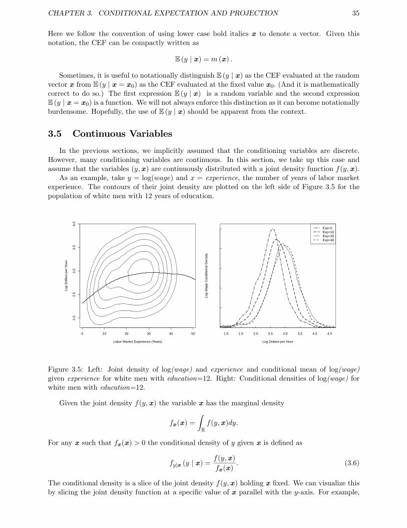
CHAPTER 3. CONDITIONAL EXPECTATION AND PROJECTION 35
Here we follow the convention of using lower case bold italics x to denote a vector. Given thisnotation, the CEF can be compactly written as
E (y | x) = m (x) .
Sometimes, it is useful to notationally distinguish E (y | x) as the CEF evaluated at the randomvector x from E (y | x = x0) as the CEF evaluated at the fixed value x0. (And it is mathematicallycorrect to do so.) The first expression E (y | x) is a random variable and the second expressionE (y | x = x0) is a function. We will not always enforce this distinction as it can become notationallyburdensome. Hopefully, the use of E (y | x) should be apparent from the context.
3.5 Continuous Variables
In the previous sections, we implicitly assumed that the conditioning variables are discrete.However, many conditioning variables are continuous. In this section, we take up this case andassume that the variables (y,x) are continuously distributed with a joint density function f(y,x).
As an example, take y = log(wage) and x = experience, the number of years of labor marketexperience. The contours of their joint density are plotted on the left side of Figure 3.5 for thepopulation of white men with 12 years of education.
Labor Market Experience (Years)
Log
Dol
lars
per
Hou
r
0 10 20 30 40 50
2.0
2.5
3.0
3.5
4.0
Log Dollars per Hour
Log
Wag
e C
ondi
tiona
l Den
sity
Exp=5Exp=10Exp=25Exp=40
1.0 1.5 2.0 2.5 3.0 3.5 4.0 4.5
Figure 3.5: Left: Joint density of log(wage) and experience and conditional mean of log(wage)given experience for white men with education=12. Right: Conditional densities of log(wage) forwhite men with education=12.
Given the joint density f(y,x) the variable x has the marginal density
fx(x) =
∫Rf(y,x)dy.
For any x such that fx(x) > 0 the conditional density of y given x is defined as
fy|x (y | x) =f(y,x)
fx(x). (3.6)
The conditional density is a slice of the joint density f(y,x) holding x fixed. We can visualize thisby slicing the joint density function at a specific value of x parallel with the y-axis. For example,
CHAPTER 3. CONDITIONAL EXPECTATION AND PROJECTION 36
take the density contours on the left side of Figure 3.5 and slice through the contour plot at aspecific value of experience. This gives us the conditional density of log(wage) for white men with12 years of education and this level of experience. We do this for four levels of experience (5, 10,25, and 40 years), and plot these densities on the right side of Figure 3.5. We can see that thedistribution of wages shifts to the right and becomes more diffuse as experience increases from 5 to10 years, and from 10 to 25 years, but there is little change from 25 to 40 years experience.
The CEF of y given x is the mean of the conditional density (3.6)
m (x) = E (y | x) =
∫Ryfy|x (y | x) dy. (3.7)
Intuitively, m (x) is the mean of y for the idealized subpopulation where the conditioning variablesare fixed at x. This is idealized since x is continuously distributed so this subpopulation is infinitelysmall.
In Figure 3.5 the CEF of log(wage) given experience is plotted as the solid line. We can seethat the CEF is a smooth but nonlinear function. The CEF is initially increasing in experience,flattens out around experience = 30, and then decreases for high levels of experience.
3.6 Law of Iterated Expectations
An extremely useful tool from probability theory is the law of iterated expectations. Animportant special case is the known as the Simple Law.
Theorem 3.6.1 Simple Law of Iterated ExpectationsIf E |y| <∞ then for any random vector x,
E (E (y | x)) = E (y)
The simple law states that the expectation of the conditional expectation is the unconditionalexpectation. In other words, the average of the conditional averages is the unconditional average.When x is discrete
E (E (y | x)) =∞∑j=1
E (y | x j) Pr (x = x j)
and when x is continuous
E (E (y | x)) =
∫RkE (y | x ) fx(x)dx.
Going back to our investigation of average log wages for men and women, the simple law statesthat
E (log(wage) | gender = man) Pr (gender = man)
+E (log(wage) | gender = woman) Pr (gender = woman)
= E (log(wage)) .
Or numerically,3.05 ∗ 0.57 + 2.79 ∗ 0.43 = 2.92.
The general law of iterated expectations allows two sets of conditioning variables.
CHAPTER 3. CONDITIONAL EXPECTATION AND PROJECTION 37
Theorem 3.6.2 Law of Iterated ExpectationsIf E |y| <∞ then for any random vectors x1 and x2,
E (E (y | x1,x2) | x1) = E (y | x1)
Notice the way the law is applied. The inner expectation conditions on x1 and x2, whilethe outer expectation conditions only on x1. The iterated expectation yields the simple answerE (y | x1) , the expectation conditional on x1 alone. Sometimes we phrase this as: “The smallerinformation set wins.”
As an example
E (log(wage) | gender = man, race = white) Pr (race = white|gender = man)
+E (log(wage) | gender = man, race = black) Pr (race = black|gender = man)
+E (log(wage) | gender = man, race = other) Pr (race = other|gender = man)
= E (log(wage) | gender = man)
or numerically3.07 ∗ 0.84 + 2.86 ∗ 0.08 + 3.05 ∗ 0.08 = 3.05
A property of conditional expectations is that when you condition on a random vector x youcan effectively treat it as if it is constant. For example, E (x | x) = x and E (g (x) | x) = g (x) forany function g(·). The general property is known as the conditioning theorem.
Theorem 3.6.3 Conditioning TheoremIf
E |g (x) y| <∞ (3.8)
thenE (g (x) y | x) = g (x)E (y | x) (3.9)
andE (g (x) y) = E (g (x)E (y | x)) (3.10)
The proofs of Theorems 3.6.1, 3.6.2 and 3.6.3 are given in Section 3.30.
3.7 Monotonicity of Conditioning
What is the effect of increasing the amount of information when constructing a conditionalexpectation? That is, how do we compare E (y | x1) versus E (y | x1,x2)? We have seen thatby increasing the conditioning set, the conditional expectation reveals greater detail about thedistribution of y. Is there something more that can be said?
It turns out that there is a simple relationship induced by conditioning. We can think ofthe conditional mean E (y | x1) as the “explained portion” of y. The remainder y − E (y | x1) isthe “unexplained portion”. The simple relationship we now derive shows that the variance ofthis unexplained portion decreases when we condition on more variables. This relationship ismonotonic in the sense that increasing the amont of information always decreases the variance ofthe unexplained portion.
CHAPTER 3. CONDITIONAL EXPECTATION AND PROJECTION 38
Theorem 3.7.1 If Ey2 <∞ then
var (y) ≥ var (y − E (y | x1)) ≥ var (y − E (y | x1,x2))
Theorem 3.7.1 says that the variance of the difference between y and its conditional mean(weakly) decreases whenever an additional variable is added to the conditioning information.
The proof of Theorem 3.7.1 is given in Section 3.30.
3.8 CEF Error
The CEF error e is defined as the difference between y and the CEF evaluated at the randomvector x:
e = y −m(x).
By construction, this yields the formula
y = m(x) + e. (3.11)
In (3.11) it is useful to understand that the error e is derived from the joint distribution of(y,x), and so its properties are derived from this construction.
A key property of the CEF error is that it has a conditional mean of zero. To see this, by thelinearity of expectations, the definition m(x) = E (y | x) and the Conditioning Theorem
E (e | x) = E ((y −m(x)) | x)
= E (y | x)− E (m(x) | x)
= m(x)−m(x)
= 0.
This fact can be combined with the law of iterated expectations to show that the unconditionalmean is also zero.
E (e) = E (E (e | x)) = E (0) = 0
We state this and some other results formally.
Theorem 3.8.1 Properties of the CEF errorIf E |y| <∞ then
1. E (e | x) = 0.
2. E (e) = 0.
3. If E |y|r <∞ for r ≥ 1 then E |e|r <∞.
4. For any function h (x) such that E |h (x) e| <∞ then E (h (x) e) = 0
The proof of the third result is deferred to Section 3.30.The fourth result, whose proof is left to Exercise 3.3, says that e is uncorrelated with any
function of the regressors.The equations
y = m(x) + e
E (e | x) = 0.
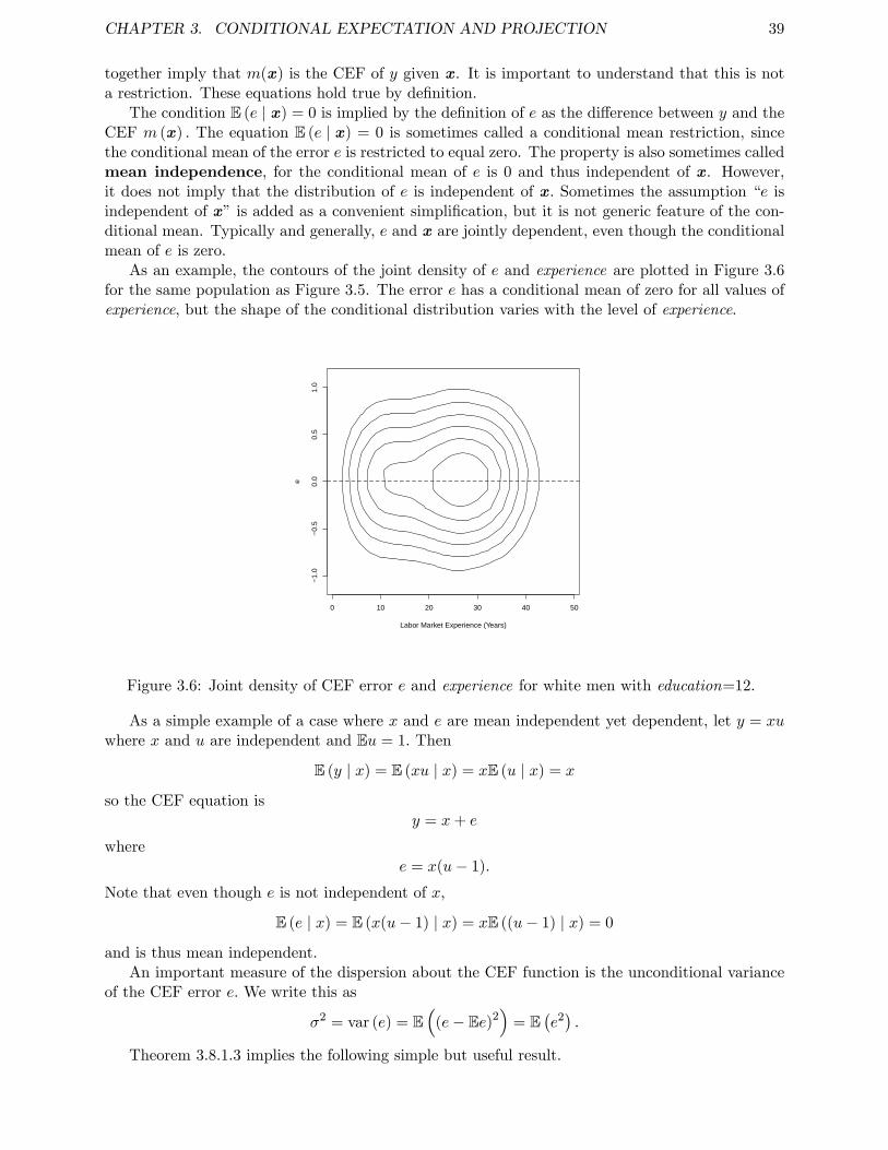
CHAPTER 3. CONDITIONAL EXPECTATION AND PROJECTION 39
together imply that m(x) is the CEF of y given x. It is important to understand that this is nota restriction. These equations hold true by definition.
The condition E (e | x) = 0 is implied by the definition of e as the difference between y and theCEF m (x) . The equation E (e | x) = 0 is sometimes called a conditional mean restriction, sincethe conditional mean of the error e is restricted to equal zero. The property is also sometimes calledmean independence, for the conditional mean of e is 0 and thus independent of x. However,it does not imply that the distribution of e is independent of x. Sometimes the assumption “e isindependent of x”is added as a convenient simplification, but it is not generic feature of the con-ditional mean. Typically and generally, e and x are jointly dependent, even though the conditionalmean of e is zero.
As an example, the contours of the joint density of e and experience are plotted in Figure 3.6for the same population as Figure 3.5. The error e has a conditional mean of zero for all values ofexperience, but the shape of the conditional distribution varies with the level of experience.
Labor Market Experience (Years)
e
0 10 20 30 40 50
−1.
0−
0.5
0.0
0.5
1.0
Figure 3.6: Joint density of CEF error e and experience for white men with education=12.
As a simple example of a case where x and e are mean independent yet dependent, let y = xuwhere x and u are independent and Eu = 1. Then
E (y | x) = E (xu | x) = xE (u | x) = x
so the CEF equation isy = x+ e
wheree = x(u− 1).
Note that even though e is not independent of x,
E (e | x) = E (x(u− 1) | x) = xE ((u− 1) | x) = 0
and is thus mean independent.An important measure of the dispersion about the CEF function is the unconditional variance
of the CEF error e. We write this as
σ2 = var (e) = E(
(e− Ee)2)
= E(e2).
Theorem 3.8.1.3 implies the following simple but useful result.
CHAPTER 3. CONDITIONAL EXPECTATION AND PROJECTION 40
Theorem 3.8.2 If Ey2 <∞ then σ2 <∞
3.9 Best Predictor
Suppose that given a realized value of x, we want to create a prediction or forecast of y.We canwrite any predictor as a function g (x) of x. The prediction error is the realized difference y−g(x).A non-stochastic measure of the magnitude of the prediction error is the expectation of its square
E (y − g (x))2 . (3.12)
We can define the best predictor as the function g (x) which minimizes (3.12). What functionis the best predictor? It turns out that the answer is the CEF m(x). This holds regardless of thejoint distribution of (y,x).
To see this, note that the mean squared error of a predictor g (x) is
E (y − g (x))2 = E (e+m (x)− g (x))2
= Ee2 + 2E (e (m (x)− g (x))) + E (m (x)− g (x))2
= Ee2 + E (m (x)− g (x))2
≥ Ee2 = E (y −m (x))2
where the first equality makes the substitution y = m(x) + e and the third equality uses Theorem3.8.1.4. The right-hand-side after the third equality is minimized by setting g (x) = m (x), yieldingthe final inequality. The minimum is finite under the assumption Ey2 <∞ as shown by Theorem3.8.2.
We state this formally in the following result.
Theorem 3.9.1 Conditional Mean as Best PredictorIf Ey2 <∞, then for any predictor g (x),
E (y − g (x))2 ≥ E (y −m (x))2
where m (x) = E (y | x).
3.10 Conditional Variance
While the conditional mean is a good measure of the location of a conditional distribution,it does not provide information about the spread of the distribution. A common measure of thedispersion is the conditional variance.
Definition 3.10.1 If Ey2 < ∞, the conditional variance of ygiven x is
σ2(x) = var (y | x)
= E(
(y − E (y | x))2 | x)
= E(e2 | x
)
CHAPTER 3. CONDITIONAL EXPECTATION AND PROJECTION 41
Generally, σ2 (x) is a non-trivial function of x and can take any form subject to the restrictionthat it is non-negative. The conditional standard deviation is its square root σ(x) =
√σ2(x).
One way to think about σ2(x) is that it is the conditional mean of e2 given x.As an example of how the conditional variance depends on observables, compare the conditional
log wage densities for men and women displayed in Figure 3.3. The difference between the densitiesis not purely a location shift, but is also a difference in spread. Specifically, we can see that thedensity for men’s log wages is somewhat more spread out than that for women, while the densityfor women’s wages is somewhat more peaked. Indeed, the conditional standard deviation for men’swages is 3.05 and that for women is 2.81. So while men have higher average wages, they are alsosomewhat more dispersed.
The unconditional error variance and the conditional variance are related by the law of iteratedexpectations
σ2 = E(e2)
= E(E(e2 | x
))= E
(σ2(x)
).
That is, the unconditional error variance is the average conditional variance.Given the conditional variance, we can define a rescaled error
ε =e
σ(x). (3.13)
We can calculate that since σ(x) is a function of x
E (ε | x) = E(
e
σ(x)| x)
=1
σ(x)E (e | x) = 0
and
var (ε | x) = E(ε2 | x
)= E
(e2
σ2(x)| x)
=1
σ2(x)E(e2 | x
)=σ2(x)
σ2(x)= 1.
Thus ε has a conditional mean of zero, and a conditional variance of 1.Notice that (3.13) can be rewritten as
e = σ(x)ε.
and substituting this for e in the CEF equation (3.11), we find that
y = m(x) + σ(x)ε. (3.14)
This is an alternative (mean-variance) representation of the CEF equation.Many econometric studies focus on the conditional mean m(x) and either ignore the condi-
tional variance σ2(x), treat it as a constant σ2(x) = σ2, or treat it as a nuisance parameter (aparameter not of primary interest). This is appropriate when the primary variation in the condi-tional distribution is in the mean, but can be short-sighted in other cases. Dispersion is relevantto many economic topics, including income and wealth distribution, economic inequality, and pricedispersion. Conditional dispersion (variance) can be a fruitful subject for investigation.
The perverse consequences of a narrow-minded focus on the mean has been parodied in a classicjoke:
An economist was standing with one foot in a bucket of boiling waterand the other foot in a bucket of ice. When asked how he felt, hereplied, “On average I feel just fine.”
Clearly, the economist in question ignored variance!
CHAPTER 3. CONDITIONAL EXPECTATION AND PROJECTION 42
3.11 Homoskedasticity and Heteroskedasticity
An important special case obtains when the conditional variance σ2(x) is a constant and inde-pendent of x. This is called homoskedasticity.
Definition 3.11.1 The error is homoskedastic if E(e2 | x
)= σ2
does not depend on x.
In the general case where σ2(x) depends on x we say that the error e is heteroskedastic.
Definition 3.11.2 The error is heteroskedastic if E(e2 | x
)= σ2(x)
depends on x.
It is helpful to understand that the concepts homoskedasticity and heteroskedasticity concernthe conditional variance, not the unconditional variance. By definition, the unconditional varianceis a constant and independent of the regressors x. So when we talk about the variance as a functionof the regressors, we are talking about the conditional variance. Recall Figure 3.3 and how thevariance of wages varies between men and women.
Some older or introductory textbooks describe heteroskedasticity as the case where “the vari-ance of e varies across observations”. This is a poor and confusing definition. It is more constructiveto understand that heteroskedasticity means that the conditional variance σ2 (x) depends on ob-servables.
Older textbooks also tend to describe homoskedasticity as a component of a correct regressionspecification, and describe heteroskedasticity as an exception or deviance. This description hasinfluenced many generations of economists, but it is unfortunately backwards. The correct viewis that heteroskedasticity is generic and “standard”, while homoskedasticity is unusual and excep-tional. The default in empirical work should be to assume that the errors are heteroskedastic, notthe converse.
In apparent contradiction to the above statement, we will still frequently impose the ho-moskedasticity assumption when making theoretical investigations into the properties of estimationand inference methods. The reason is that in many cases homoskedasticity greatly simplifies thetheoretical calculations, and it is therefore quite advantageous for teaching and learning. It shouldalways be remembered, however, that homoskedasticity is never imposed because it is believed tobe a correct feature of an empirical model, but rather because of its simplicity.
3.12 Regression Derivative
One way to interpret the CEF m(x) = E (y | x) is in terms of how marginal changes in theregressors x imply changes in the conditional mean of the response variable y. It is typical toconsider marginal changes in single regressors, holding the remainder fixed. When a regressor x1
is continuously distributed, we define the marginal effect of a change in x1, holding the variablesx2, ..., xk fixed, as the partial derivative of the CEF
∂
∂x1m(x1, ..., xk).
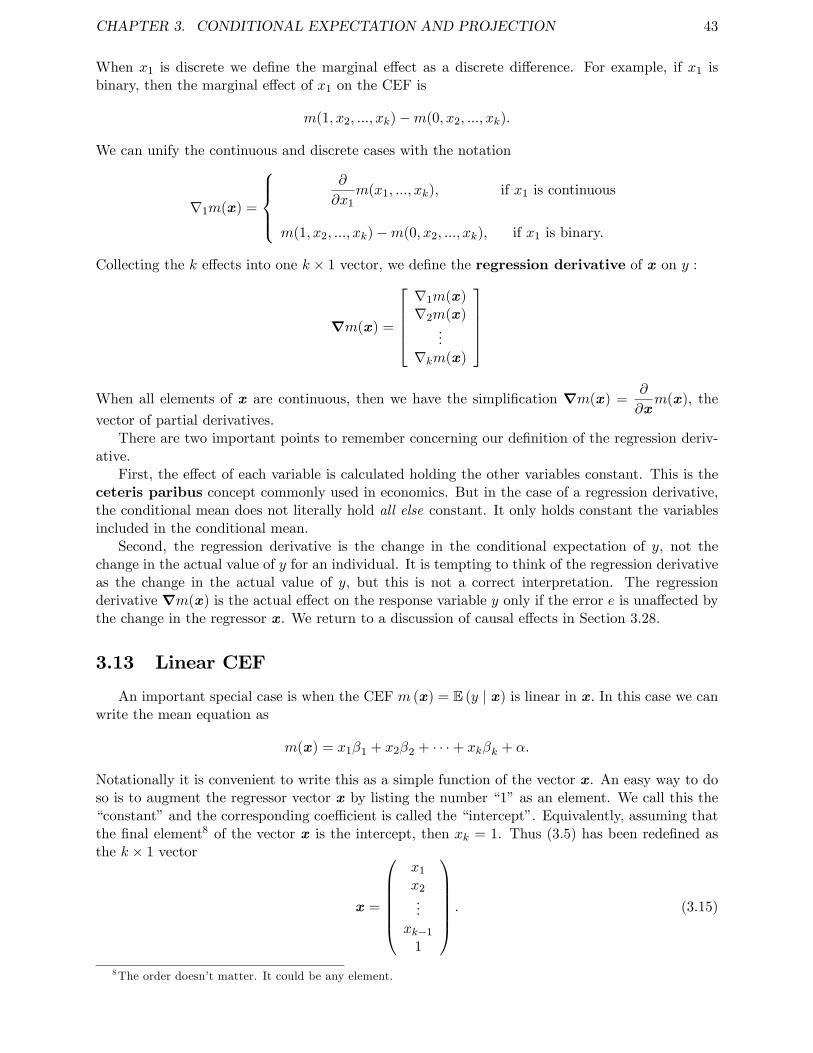
CHAPTER 3. CONDITIONAL EXPECTATION AND PROJECTION 43
When x1 is discrete we define the marginal effect as a discrete difference. For example, if x1 isbinary, then the marginal effect of x1 on the CEF is
m(1, x2, ..., xk)−m(0, x2, ..., xk).
We can unify the continuous and discrete cases with the notation
∇1m(x) =
∂
∂x1m(x1, ..., xk), if x1 is continuous
m(1, x2, ..., xk)−m(0, x2, ..., xk), if x1 is binary.
Collecting the k effects into one k × 1 vector, we define the regression derivative of x on y :
∇m(x) =
∇1m(x)∇2m(x)
...∇km(x)
When all elements of x are continuous, then we have the simplification ∇m(x) =
∂
∂xm(x), the
vector of partial derivatives.There are two important points to remember concerning our definition of the regression deriv-
ative.First, the effect of each variable is calculated holding the other variables constant. This is the
ceteris paribus concept commonly used in economics. But in the case of a regression derivative,the conditional mean does not literally hold all else constant. It only holds constant the variablesincluded in the conditional mean.
Second, the regression derivative is the change in the conditional expectation of y, not thechange in the actual value of y for an individual. It is tempting to think of the regression derivativeas the change in the actual value of y, but this is not a correct interpretation. The regressionderivative ∇m(x) is the actual effect on the response variable y only if the error e is unaffected bythe change in the regressor x. We return to a discussion of causal effects in Section 3.28.
3.13 Linear CEF
An important special case is when the CEF m (x) = E (y | x) is linear in x. In this case we canwrite the mean equation as
m(x) = x1β1 + x2β2 + · · ·+ xkβk + α.
Notationally it is convenient to write this as a simple function of the vector x. An easy way to doso is to augment the regressor vector x by listing the number “1”as an element. We call this the“constant”and the corresponding coeffi cient is called the “intercept”. Equivalently, assuming thatthe final element8 of the vector x is the intercept, then xk = 1. Thus (3.5) has been redefined asthe k × 1 vector
x =
x1
x2...
xk−1
1
. (3.15)
8The order doesn’t matter. It could be any element.
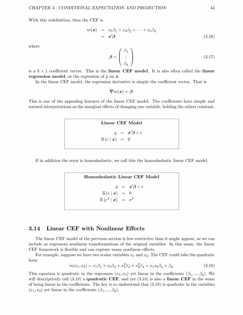
CHAPTER 3. CONDITIONAL EXPECTATION AND PROJECTION 44
With this redefinition, then the CEF is
m(x) = x1β1 + x2β2 + · · ·+ xkβk
= x′β (3.16)
where
β =
β1...βk
(3.17)
is a k × 1 coeffi cient vector. This is the linear CEF model. It is also often called the linearregression model, or the regression of y on x.
In the linear CEF model, the regression derivative is simply the coeffi cient vector. That is
∇m(x) = β.
This is one of the appealing features of the linear CEF model. The coeffi cients have simple andnatural interpretations as the marginal effects of changing one variable, holding the others constant.
Linear CEF Model
y = x′β + e
E (e | x) = 0
If in addition the error is homoskedastic, we call this the homoskedastic linear CEF model.
Homoskedastic Linear CEF Model
y = x′β + e
E (e | x) = 0
E(e2 | x
)= σ2
3.14 Linear CEF with Nonlinear Effects
The linear CEF model of the previous section is less restrictive than it might appear, as we caninclude as regressors nonlinear transformations of the original variables. In this sense, the linearCEF framework is flexible and can capture many nonlinear effects.
For example, suppose we have two scalar variables x1 and x2. The CEF could take the quadraticform
m(x1, x2) = x1β1 + x2β2 + x21β3 + x2
2β4 + x1x2β5 + β6. (3.18)
This equation is quadratic in the regressors (x1, x2) yet linear in the coeffi cients (β1, ..., β6). Wewill descriptively call (3.18) a quadratic CEF, and yet (3.18) is also a linear CEF in the senseof being linear in the coeffi cients. The key is to understand that (3.18) is quadratic in the variables(x1, x2) yet linear in the coeffi cients (β1, ..., β6).
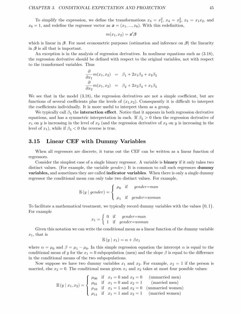
CHAPTER 3. CONDITIONAL EXPECTATION AND PROJECTION 45
To simplify the expression, we define the transformations x3 = x21, x4 = x2
2, x5 = x1x2, andx6 = 1, and redefine the regressor vector as x = (x1, ..., x6). With this redefinition,
m(x1, x2) = x′β
which is linear in β. For most econometric purposes (estimation and inference on β) the linearityin β is all that is important.
An exception is in the analysis of regression derivatives. In nonlinear equations such as (3.18),the regression derivative should be defined with respect to the original variables, not with respectto the transformed variables. Thus
∂
∂x1m(x1, x2) = β1 + 2x1β3 + x2β5
∂
∂x2m(x1, x2) = β2 + 2x2β4 + x1β5
We see that in the model (3.18), the regression derivatives are not a simple coeffi cient, but arefunctions of several coeffi cients plus the levels of (x1,x2). Consequently it is diffi cult to interpretthe coeffi cients individually. It is more useful to interpret them as a group.
We typically call β5 the interaction effect. Notice that it appears in both regression derivativeequations, and has a symmetric interpretation in each. If β5 > 0 then the regression derivative ofx1 on y is increasing in the level of x2 (and the regression derivative of x2 on y is increasing in thelevel of x1), while if β5 < 0 the reverse is true.
3.15 Linear CEF with Dummy Variables
When all regressors are discrete, it turns out the CEF can be written as a linear function ofregressors.
Consider the simplest case of a single binary regressor. A variable is binary if it only takes twodistinct values. (For example, the variable gender.) It is common to call such regressors dummyvariables, and sometimes they are called indicator variables. When there is only a single dummyregressor the conditional mean can only take two distinct values. For example,
E (y | gender) =
µ0 if gender=man
µ1 if gender=woman
To facilitate a mathematical treatment, we typically record dummy variables with the values 0, 1.For example
x1 =
0 if gender=man1 if gender=woman
Given this notation we can write the conditional mean as a linear function of the dummy variablex1, that is
E (y | x1) = α+ βx1
where α = µ0 and β = µ1 − µ0. In this simple regression equation the intercept α is equal to theconditional mean of y for the x1 = 0 subpopulation (men) and the slope β is equal to the differencein the conditional means of the two subpopulations.
Now suppose we have two dummy variables x1 and x2. For example, x2 = 1 if the person ismarried, else x2 = 0. The conditional mean given x1 and x2 takes at most four possible values:
E (y | x1, x2) =
µ00 if x1 = 0 and x2 = 0 (unmarried men)µ01 if x1 = 0 and x2 = 1 (married men)µ10 if x1 = 1 and x2 = 0 (unmarried women)µ11 if x1 = 1 and x2 = 1 (married women)
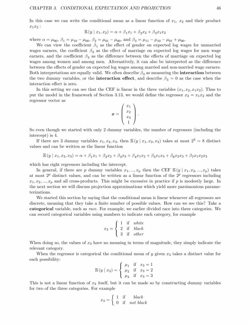
CHAPTER 3. CONDITIONAL EXPECTATION AND PROJECTION 46
In this case we can write the conditional mean as a linear function of x1, x2 and their productx1x2 :
E (y | x1, x2) = α+ β1x1 + β2x2 + β3x1x2
where α = µ00, β1 = µ10 − µ00, β2 = µ01 − µ00, and β3 = µ11 − µ10 − µ01 + µ00.We can view the coeffi cient β1 as the effect of gender on expected log wages for unmarried
wages earners, the coeffi cient β2 as the effect of marriage on expected log wages for men wageearners, and the coeffi cient β3 as the difference between the effects of marriage on expected logwages among women and among men. Alternatively, it can also be interpreted as the differencebetween the effects of gender on expected log wages among married and non-married wage earners.Both interpretations are equally valid. We often describe β3 as measuring the interaction betweenthe two dummy variables, or the interaction effect, and describe β3 = 0 as the case when theinteraction effect is zero.
In this setting we can see that the CEF is linear in the three variables (x1, x2, x1x2). Thus toput the model in the framework of Section 3.13, we would define the regressor x3 = x1x2 and theregressor vector as
x =
x1
x2
x3
1
.
So even though we started with only 2 dummy variables, the number of regressors (including theintercept) is 4.
If there are 3 dummy variables x1, x2, x3, then E (y | x1, x2, x3) takes at most 23 = 8 distinctvalues and can be written as the linear function
E (y | x1, x2, x3) = α+ β1x1 + β2x2 + β3x3 + β4x1x2 + β5x1x3 + β6x2x3 + β7x1x2x3
which has eight regressors including the intercept.In general, if there are p dummy variables x1, ..., xp then the CEF E (y | x1, x2, ..., xp) takes
at most 2p distinct values, and can be written as a linear function of the 2p regressors includingx1, x2, ..., xp and all cross-products. This might be excessive in practice if p is modestly large. Inthe next section we will discuss projection approximations which yield more parsimonious parame-terizations.
We started this section by saying that the conditional mean is linear whenever all regressors arediscrete, meaning that they take a finite number of possible values. How can we see this? Take acategorical variable, such as race. For example, we earlier divided race into three categories. Wecan record categorical variables using numbers to indicate each category, for example
x3 =
1 if white2 if black3 if other
When doing so, the values of x3 have no meaning in terms of magnitude, they simply indicate therelevant category.
When the regressor is categorical the conditional mean of y given x3 takes a distinct value foreach possibility:
E (y | x3) =
µ1 if x3 = 1µ2 if x3 = 2µ3 if x3 = 3
This is not a linear function of x3 itself, but it can be made so by constructing dummy variablesfor two of the three categories. For example
x4 =
1 if black0 if not black
CHAPTER 3. CONDITIONAL EXPECTATION AND PROJECTION 47
x5 =
1 if other0 if not other
In this case, the categorical variable x3 is equivalent to the pair of dummy variables (x4, x5). Theexplicit relationship is
x3 =
1 if x4 = 0 and x5 = 02 if x4 = 1 and x5 = 03 if x4 = 0 and x5 = 1
Given these transformations, we can write the conditional mean of y as a linear function of x4 andx5
E (y | x3) = E (y | x4, x5) = α+ β1x4 + β2x5
We can write the CEF as either E (y | x3) or E (y | x4, x5) (they are equivalent), but it is only linearas a function of x4 and x5.
This setting is similar to the case of two dummy variables, with the difference that we have notincluded the interaction term x4x5. This is because the event x4 = 1 and x5 = 1 is empty byconstruction, so x4x5 = 0 by definition.
3.16 Best Linear Predictor
While the conditional mean m(x) = E (y | x) is the best predictor of y among all functionsof x, its functional form is typically unknown. In particular, the linear CEF model is empiricallyunlikely to be accurate unless x is discrete and low-dimensional so all interactions are included.Consequently in most cases it is more realistic to view the linear specification (3.16) as an approx-imation. In this section we derive a specific approximation with a simple interpretation.
Theorem 3.9.1 showed that the conditional mean m (x) is the best predictor in the sense thatit has the lowest mean squared error among all predictors. By extension, we can define an approx-imation to the CEF by the linear function with the lowest mean squared error among all linearpredictors.
For this derivation we require the following regularity condition.
Assumption 3.16.1
1. Ey2 <∞.
2. E ‖x‖2 <∞.
3. Qxx = E (xx′) is positive definite.
The first two parts of Assumption 3.16.1 imply that the variables y and x have finite means,variances, and covariances. The third part of the assumption is more technical, and its role willbecome apparent shortly. It is equivalent to imposing that the columns of Qxx = E (xx′) arelinearly independent, or equivalently that the matrix Qxx is invertible.
A linear predictor for y is a function of the form x′β for some β ∈ Rk. The mean squaredprediction error is
S(β) = E(y − x′β
)2.
The best linear predictor of y given x, written P(y | x), is found by selecting the vector β tominimize S(β).
CHAPTER 3. CONDITIONAL EXPECTATION AND PROJECTION 48
Definition 3.16.1 The Best Linear Predictor of y given x is
P(y | x) = x′β
where β minimizes the mean squared prediction error
S(β) = E(y − x′β
)2.
The minimizerβ = argmin
β∈RkS(β) (3.19)
is called the Linear Projection Coeffi cient.
We now calculate an explicit expression for its value.The mean squared prediction error can be written out as a quadratic function of β :
S(β) = Ey2 − 2β′E (xy) + β′E(xx′
)β.
The quadratic structure of S(β) means that we can solve explicitly for the minimizer. The first-order condition for minimization (from Appendix A.9) is
0 =∂
∂βS(β) = −2E (xy) + 2E
(xx′)β. (3.20)
Rewriting (3.20) as2E (xy) = 2E
(xx′)β
and dividing by 2, this equation takes the form
Qxy = Qxxβ (3.21)
where Qxy = E (xy) is k × 1 and Qxx = E (xx′) is k × k. The solution is found by inverting thematrix Qxx, and is written
β = Q−1xxQxy
orβ =
(E(xx′))−1 E (xy) . (3.22)
It is worth taking the time to understand the notation involved in the expression (3.22). Qxx is ak × k matrix and Qxy is a k × 1 column vector. Therefore, alternative expressions such as E(xy)
E(xx′)
or E (xy) (E (xx′))−1 are incoherent and incorrect. We also can now see the role of Assumption3.16.1.3. It is necessary in order for the solution (3.22) to exist. Otherwise, there would be multiplesolutions to the equation (3.21).
We now have an explicit expression for the best linear predictor:
P(y | x) = x′(E(xx′))−1 E (xy) .
This expression is also referred to as the linear projection of y on x.The projection error is
e = y − x′β. (3.23)
This equals the error from the regression equation when (and only when) the conditional mean islinear in x, otherwise they are distinct.
CHAPTER 3. CONDITIONAL EXPECTATION AND PROJECTION 49
Rewriting, we obtain a decomposition of y into linear predictor and error
y = x′β + e. (3.24)
In general we call equation (3.24) or x′β the best linear predictor of y given x, or the linearprojection of y on x. Equation (3.24) is also often called the regression of y on x but this cansometimes be confusing as economists use the term regression in many contexts. (Recall that wesaid in Section 3.13 that the linear CEF model is also called the linear regression model.)
An important property of the projection error e is
E (xe) = 0. (3.25)
To see this, using the definitions (3.23) and (3.22) and the matrix properties AA−1 = I andIa = a,
E (xe) = E(x(y − x′β
))= E (xy)− E
(xx′) (E(xx′))−1 E (xy)
= 0 (3.26)
as claimed.Equation (3.25) is a set of k equations, one for each regressor. In other words, (3.25) is equivalent
toE (xje) = 0 (3.27)
for j = 1, ..., k. As in (3.15), the regressor vector x typically contains a constant, e.g. xk = 1. Inthis case (3.27) for j = k is the same as
E (e) = 0. (3.28)
Thus the projection error has a mean of zero when the regressor vector contains a constant. (Whenx does not have a constant, (3.28) is not guaranteed. As it is desirable for e to have a zero mean,this is a good reason to always include a constant in any model.)
It is also useful to observe that since cov(xj , e) = E (xje) − E (xj)E (e) , then (3.27)-(3.28)together imply that the variables xj and e are uncorrelated.
This completes the derivation of the model. We summarize some of the most important prop-erties.
CHAPTER 3. CONDITIONAL EXPECTATION AND PROJECTION 50
Theorem 3.16.1 Properties of Linear Projection ModelUnder Assumption 3.16.1,
1. The moments E (xx′) and E (xy) exist with finite elements.
2. The Linear Projection Coeffi cient (3.19) exists, is unique, and equals
β =(E(xx′))−1 E (xy) .
3. The best linear predictor of y given x is
P(y | x) = x′(E(xx′))−1 E (xy) .
4. The projection error e = y − x′β exists and satisfies
E(e2)<∞
andE (xe) = 0.
5. If x contains an constant, then
E (e) = 0.
6. If E ‖y‖r <∞ and E ‖x‖r <∞ for r ≥ 1 then E |e|r <∞.
A complete proof of Theorem 3.16.1 is given in Section 3.30.It is useful to reflect on the generality of Theorem 3.16.1. The only restriction is Assumption
3.16.1. Thus for any random variables (y,x) with finite variances we can define a linear equation(3.24) with the properties listed in Theorem 3.16.1. Stronger assumptions (such as the linear CEFmodel) are not necessary. In this sense the linear model (3.24) exists quite generally. However,it is important not to misinterpret the generality of this statement. The linear equation (3.24) isdefined as the best linear predictor. It is not necessarily a conditional mean, nor a parameter of astructural or causal economic model.
Linear Projection Model
y = x′β + e.
E (xe) = 0
β =(E(xx′))−1 E (xy)
We illustrate projection using three log wage equations introduced in earlier sections.For our first example, we consider a model with the two dummy variables for gender and race
similar to Table 3.1. As we learned in Section 3.15, the entries in this table can be equivalentlyexpressed by a linear CEF. For simplicity, let’s consider the CEF of ln(wage) as a function of Blackand Female.
E(log(wage) | Black, Female) = −0.20Black − 0.24Female+ 0.10Black ∗ Female+ 3.06.
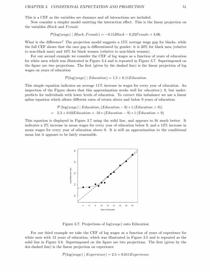
CHAPTER 3. CONDITIONAL EXPECTATION AND PROJECTION 51
This is a CEF as the variables are dummys and all interactions are included.Now consider a simpler model omitting the interaction effect. This is the linear projection on
the variables Black and Female
P(log(wage) | Black, Female) = −0.15Black − 0.23Female+ 3.06.
What is the difference? The projection model suggests a 15% average wage gap for blacks, whilethe full CEF shows that the race gap is differentiated by gender: it is 20% for black men (relativeto non-black men) and 10% for black women (relative to non-black women).
For our second example we consider the CEF of log wages as a function of years of educationfor white men which was illustrated in Figure 3.4 and is repeated in Figure 3.7. Superimposed onthe figure are two projections. The first (given by the dashed line) is the linear projection of logwages on years of education
P(log(wage) | Education) = 1.5 + 0.11Education
This simple equation indicates an average 11% increase in wages for every year of education. Aninspection of the Figure shows that this approximation works well for education≥ 9, but under-predicts for individuals with lower levels of education. To correct this imbalance we use a linearspline equation which allows different rates of return above and below 9 years of education:
P (log(wage) | Education, (Education− 9) ∗ 1 (Education > 9))
= 2.3 + 0.02Education+ .10 ∗ (Education− 9) ∗ 1 (Education > 9)
This equation is displayed in Figure 3.7 using the solid line, and appears to fit much better. Itindicates a 2% increase in mean wages for every year of education below 9, and a 12% increase inmean wages for every year of education above 9. It is still an approximation to the conditionalmean but it appears to be fairly reasonable.
2.0
2.5
3.0
3.5
4.0
Years of Education
Log
Dol
lars
per
Hou
r
4 6 8 10 12 14 16 18 20
Figure 3.7: Projections of log(wage) onto Education
For our third example we take the CEF of log wages as a function of years of experience forwhite men with 12 years of education, which was illustrated in Figure 3.5 and is repeated as thesolid line in Figure 3.8. Superimposed on the figure are two projections. The first (given by thedot-dashed line) is the linear projection on experience
P(log(wage) | Experience) = 2.5 + 0.011Experience
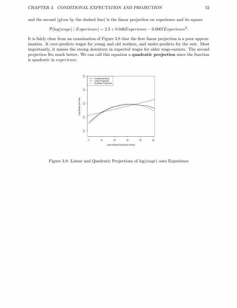
CHAPTER 3. CONDITIONAL EXPECTATION AND PROJECTION 52
and the second (given by the dashed line) is the linear projection on experience and its square
P(log(wage) | Experience) = 2.3 + 0.046Experience− 0.0007Experience2.
It is fairly clear from an examination of Figure 3.8 that the first linear projection is a poor approx-imation. It over-predicts wages for young and old workers, and under-predicts for the rest. Mostimportantly, it misses the strong downturn in expected wages for older wage-earners. The secondprojection fits much better. We can call this equation a quadratic projection since the functionis quadratic in experience.
0 10 20 30 40 50
2.0
2.5
3.0
3.5
4.0
Labor Market Experience (Years)
Log
Dol
lars
per
Hou
rConditional MeanLinear ProjectionQuadratic Projection
Figure 3.8: Linear and Quadratic Projections of log(wage) onto Experience
CHAPTER 3. CONDITIONAL EXPECTATION AND PROJECTION 53
Invertibility and Identification
The linear projection coeffi cient β = (E (xx′))−1 E (xy) exists and is unique as longas the k × k matrix Qxx = E (xx′) is invertible. The matrix Qxx is sometimes calledthe design matrix, as in experimental settings the researcher is able to control Qxx bymanipulating the distribution of the regressors x.
Observe that for any non-zero α ∈ Rk,
α′Qxxα = E(α′xx′α
)= E
(α′x
)2 ≥ 0
soQxx by construction is positive semi-definite. The assumption that it is positive definitemeans that this is a strict inequality, E (α′x)2 > 0. Equivalently, there cannot exist a non-zero vector α such that α′x = 0 identically. This occurs when redundant variables areincluded in x. Positive semi-definite matrices are invertible if and only if they are positivedefinite. When Qxx is invertible then β = (E (xx′))−1 E (xy) exists and is uniquelydefined. In other words, in order for β to be uniquely defined, we must exclude thedegenerate situation of redundant varibles.
Theorem 3.16.1 shows that the linear projection coeffi cient β is identified (uniquelydetermined) under Assumptions 3.16.1. The key is invertibility of Qxx. Otherwise, thereis no unique solution to the equation
Qxxβ = Qxy. (3.29)
When Qxx is not invertible there are multiple solutions to (3.29), all of which yield anequivalent best linear predictor x′β. In this case the coeffi cient β is not identified as itdoes not have a unique value. Even so, the best linear predictor x′β still identified. Onesolution is to set
β =(E(xx′))− E (xy)
where A− denotes the generalized inverse of A (see Appendix A.5).
3.17 Linear Predictor Error Variance
As in the CEF model, we define the error variance as
σ2 = E(e2).
Setting Qyy = E(y2)and Qyx = E (yx′) we can write σ2 as
σ2 = E(y − x′β
)2= Ey2 − 2E
(yx′)β + β′E
(xx′)β
= Qyy − 2QyxQ−1xxQxy +QyxQ
−1xxQxxQ
−1xxQxy
= Qyy −QyxQ−1xxQxy
def= Qyy·x (3.30)
One useful feature of this formula is that it shows that Qyy·x = Qyy − QyxQ−1xxQxy equals the
variance of the error from the linear projection of y on x.
CHAPTER 3. CONDITIONAL EXPECTATION AND PROJECTION 54
3.18 Regression Coeffi cients
Sometimes it is useful to separate the intercept from the other regressors, and write the linearprojection equation in the format
y = α+ x′β + e (3.31)
where α is the intercept and x does not contain a constant.Taking expectations of this equation, we find
Ey = Eα+ Ex′β + Ee
orµy = α+ µ′xβ
where µy = Ey and µx = Ex, since E (e) = 0 from (3.28). Rearranging, we find
α = µy − µ′xβ.
Subtracting this equation from (3.31) we find
y − µy = (x− µx)′ β + e, (3.32)
a linear equation between the centered variables y − µy and x − µx. (They are centered at theirmeans, so are mean-zero random variables.) Because x − µx is uncorrelated with e, (3.32) is alsoa linear projection, thus by the formula for the linear projection model,
β =(E((x− µx) (x− µx)′
))−1 E((x− µx)
(y − µy
))= var (x)−1 cov (x, y)
a function only of the covariances9 of x and y.
Theorem 3.18.1 In the linear projection model
y = α+ x′β + e,
thenα = µy − µ′xβ (3.33)
andβ = var (x)−1 cov (x, y) . (3.34)
3.19 Regression Sub-Vectors
Let the regressors be partitioned as
xi =
(x1i
x2i
). (3.35)
9The covariance matrix between vectors x and z is cov (x,z) = E((x− Ex) (z − Ez)′
). The (co)variance
matrix of the vector x is var (x) = cov (x,z) = E((x− Ex) (x− Ex)′
).
CHAPTER 3. CONDITIONAL EXPECTATION AND PROJECTION 55
We can write the projection of yi on xi as
yi = x′iβ + ei
= x′1iβ1 + x′2iβ2 + ei (3.36)
E (xiei) = 0.
In this section we derive formula for the sub-vectors β1 and β2.Partition Qxx comformably with xi
Qxx =
[Q11 Q12
Q21 Q22
]=
[E (x1ix
′1i) E (x1ix
′2i)
E (x2ix′1i) E (x2ix
′2i)
]and similarly Qxy
Qxy =
[Q1y
Q2y
]=
[E (x1iyi)E (x2iyi)
].
By the partitioned matrix inversion formula (A.4)
Q−1xx =
[Q11 Q12
Q21 Q22
]−1def=
[Q11 Q12
Q21 Q22
]=
[Q−1
11·2 −Q−111·2Q12Q
−122
−Q−122·1Q21Q
−111 Q−1
22·1
]. (3.37)
where Q11·2def= Q11 −Q12Q
−122 Q21 and Q22·1
def= Q22 −Q21Q
−111 Q12. Thus
β =
(β1
β2
)=
[Q−1
11·2 −Q−111·2Q12Q
−122
−Q−122·1Q21Q
−111 Q−1
22·1
] [Q1y
Q2y
]=
(Q−1
11·2(Q1y −Q12Q
−122 Q2y
)Q−1
22·1(Q2y −Q21Q
−111 Q1y
) )=
(Q−1
11·2Q1y·2Q−1
22·1Q2y·1
)We have shown that
β1 = Q−111·2Q1y·2
β2 = Q−122·1Q2y·1
3.20 Coeffi cient Decomposition
In the previous section we derived formula for the coeffi cient sub-vectors β1 and β2. We nowuse these formula to give a useful interpretation of the coeffi cients as obtaining from an interatedprojection.
Take equation (3.36) for the case dim(x1i) = 1 so that β1 ∈ R.
yi = x1iβ1 + x′2iβ2 + ei. (3.38)
Now consider the projection of x1i on x2i :
x1i = x′2iγ2 + u1i
E (x2iu1i) = 0.
From (3.22) and (3.30), γ2 = Q−122 Q21 and Eu2
1i = Q11·2. We can also calculate that
E (u1iyi) = E((x1i − γ ′2x2i
)yi)
= E (x1iyi)− γ ′2E (x2iyi) = Q1y −Q12Q−122 Q2y = Q1y·2.
CHAPTER 3. CONDITIONAL EXPECTATION AND PROJECTION 56
We have found that
β1 = Q−111·2Q1y·2 =
E (u1iyi)
Eu21i
the coeffi cient from the simple regression of yi on u1i.What this means is that in the multivariate projection equation (3.38), the coeffi cient β1 equals
the projection coeffi cient from a regression of yi on u1i, the error from a projection of x1i on theother regressors x2i. The error u1i can be thought of as the component of x1i which is not linearlyexplained by the other regressors. Thus the the coeffi cient β1 equals the linear effect of x1i on yi,after stripping out the effects of the other variables.
There was nothing special in the choice of the variable x1i. So this derivation applies symmet-rically to all coeffi cients in a linear projection. Each coeffi cient equals the simple regression of yion the error from a projection of that regressor on all the other regressors. Each coeffi cient equalsthe linear effect of that variable on yi, after linearly controlling for all the other regressors.
3.21 Omitted Variable Bias
Again, let the regressors be partitioned as in (3.35). Consider the projection of yi on x1i only.Perhaps this is done because the variables x2i are not observed. This is the equation
yi = x′1iγ1 + ui (3.39)
E (x1iui) = 0
Notice that we have written the coeffi cient on x1i as γ1 rather than β1 and the error as ui ratherthan ei. This is because (3.39) is different than (3.36). Goldberger (1991) introduced the catchylabels long regression for (3.36) and short regression for (3.39) to emphasize the distinction.
Typically, β1 6= γ1, except in special cases. To see this, we calculate
γ1 =(E(x1ix
′1i
))−1 E (x1iyi)
=(E(x1ix
′1i
))−1 E(x1i
(x′1iβ1 + x′2iβ2 + ei
))= β1 +
(E(x1ix
′1i
))−1 E(x1ix
′2i
)β2
= β1 + Γβ2
whereΓ =
(E(x1ix
′1i
))−1 E(x1ix
′2i
)is the coeffi cient matrix from a projection of x2i on x1i.
Observe that γ1 = β1 + Γβ2 6= β1 unless Γ = 0 or β2 = 0. Thus the short and long regressionshave different coeffi cients on x1i. They are the same only under one of two conditions. First, if theprojection of x2i on x1i yields a set of zero coeffi cients (they are uncorrelated), or second, if thecoeffi cient on x2i in (3.36) is zero. In general, the coeffi cient in (3.39) is γ1 rather than β1. Thedifference Γβ2 between γ1 and β1 is known as omitted variable bias. It is the consequence ofomission of a relevant correlated variable.
To avoid omitted variables bias the standard advice is to include all potentially relevant variablesin estimated models. By construction, the general model will be free of the omitted variablesproblem. Typically it is not feasible to completely follow this advice as many desired variables arenot observed. In this case, the possibility of omitted variables bias should be acknowledged anddiscussed in the course of an empirical investigation.
CHAPTER 3. CONDITIONAL EXPECTATION AND PROJECTION 57
3.22 Best Linear Approximation
There are alternative ways we could construct a linear approximation x′β to the conditionalmean m(x). In this section we show that one natural approach turns out to yield the same answeras the best linear predictor.
We start by defining the mean-square approximation error of x′β to m(x) as the expectedsquared difference between x′β and the conditional mean m(x)
d(β) = E(m(x)− x′β
)2. (3.40)
The function d(β) is a measure of the deviation of x′β from m(x). If the two functions are identicalthen d(β) = 0, otherwise d(β) > 0.We can also view the mean-square difference d(β) as a density-weighted average of the function (m(x)− x′β)2 , since
d(β) =
∫Rk
(m(x)− x′β
)2fx(x)dx
where fx(x) is the marginal density of x.We can then define the best linear approximation to the conditional m(x) as the function x′β
obtained by selecting β to minimize d(β) :
β = argminβ∈Rk
d(β). (3.41)
Similar to the best linear predictor we are measuring accuracy by expected squared error. Thedifference is that the best linear predictor (3.19) selects β to minimize the expected squared predic-tion error, while the best linear approximation (3.41) selects β to minimize the expected squaredapproximation error.
Despite the different definitions, it turns out that the best linear predictor and the best linearapproximation are identical. By the same steps as in (3.16) plus an application of conditionalexpectations we can find that
β =(E(xx′))−1 E (xm(x)) (3.42)
=(E(xx′))−1 E (xy) (3.43)
(see Exercise 3.18). Thus (3.41) equals (3.19). We conclude that the definition (3.41) can be viewedas an alternative motivation for the linear projection coeffi cient.
3.23 Normal Regression
Suppose the variables (y,x) are jointly normally distributed. Consider the best linear predictorof y given x
y = x′β + e
β =(E(xx′))−1 E (xy) .
Since the error e is a linear transformation of the normal vector (y,x), it follows that (e,x) isjointly normal, and since they are jointly normal and uncorrelated (since E (xe) = 0) they are alsoindependent (see Appendix B.9). Independence implies that
E (e | x) = E (e) = 0
andE(e2 | x
)= E
(e2)
= σ2
CHAPTER 3. CONDITIONAL EXPECTATION AND PROJECTION 58
which are properties of a homoskedastic linear CEF.We have shown that when (y,x) are jointly normal, they satisfy a normal linear CEF
y = x′β + e
wheree ∼ N(0, σ2)
is independent of x.This is an alternative (and traditional) motivation for the linear CEF model. This motivation
has limited merit in econometric applications since economic data is typically non-normal.
3.24 Regression to the Mean
The term regression originated in an influential paper by Francis Galton published in 1886,where he examined the joint distribution of the stature (height) of parents and children. Effectively,he was estimating the conditional mean of children’s height given their parents height. Galtondiscovered that this conditional mean was approximately linear with a slope of 2/3. This impliesthat on average a child’s height is more mediocre than his or her parent’s height. Galton calledthis phenomenon regression to the mean, and the label regression has stuck to this day todescribe most conditional relationships.
One of Galton’s fundamental insights was to recognize that if the marginal distributions of yand x are the same (e.g. the heights of children and parents in a stable environment) then theregression slope in a linear projection is always less than one.
To be more precise, take the simple linear projection
y = α+ xβ + e (3.44)
where y equals the height of the child and x equals the height of the parent. Assume that y and xhave the same mean, so that µy = µx = µ. Then from (3.33)
α = (1− β)µ
so we can write the linear projection (3.44) as
P (y | x) = (1− β)µ+ xβ.
This shows that the projected height of the child is a weighted average of the population averageheight µ and the parent’s height x, with the weight equal to the regression slope β. When theheight distribution is stable across generations, so that var(y) = var(x), then this slope is thesimple correlation of y and x. Using (3.34)
β =cov (x, y)
var(x)= corr(x, y).
By the properties of correlation (e.g. equation (B.7) in the Appendix), −1 ≤ corr(x, y) ≤ 1, withcorr(x, y) = 1 only in the degenerate case y = x. Thus if we exclude degeneracy, β is strictly lessthan 1.
This means that on average a child’s height is more mediocre (closer to the population average)than the parent’s.
CHAPTER 3. CONDITIONAL EXPECTATION AND PROJECTION 59
Sir Francis Galton
Sir Francis Galton (1822-1911) of England was one of the leading figures in late 19th centurystatistics. In addition to inventing the concept of regression, he is credited with introducingthe concepts of correlation, the standard deviation, and the bivariate normal distribution.His work on heredity made a significant intellectual advance by examing the joint distribu-tions of observables, allowing the application of the tools of mathematical statistics to thesocial sciences.
A common error —known as the regression fallacy —is to infer from β < 1 that the populationis converging, meaning that its variance is declining towards zero. This is a fallacy because we haveshown that under the assumption of constant (e.g. stable, non-converging) means and variances,the slope coeffi cient must be less than one. It cannot be anything else. A slope less than one doesnot imply that the variance of y is less than than the variance of x.
Another way of seeing this is to examine the conditions for convergence in the context of equation(3.44). Since x and e are uncorrelated, it follows that
var(y) = β2 var(x) + var(e).
Then var(y) < var(x) if and only if
β2 < 1− var(e)
var(x)
which is not implied by the simple condition |β| < 1.The regression fallacy arises in related empirical situations. Suppose you sort families into groups
by the heights of the parents, and then plot the average heights of each subsequent generation overtime. If the population is stable, the regression property implies that the plots lines will converge—children’s height will be more average than their parents. The regression fallacy is to incorrectlyconclude that the population is converging. The message is that such plots are misleading forinferences about convergence.
The regression fallacy is subtle. It is easy for intelligent economists to succumb to its temptation.A famous example is The Triumph of Mediocrity in Business by Horace Secrist, published in 1933.In this book, Secrist carefully and with great detail documented that in a sample of departmentstores over 1920-1930, when he divided the stores into groups based on 1920-1921 profits, andplotted the average profits of these groups for the subsequent 10 years, he found clear and persuasiveevidence for convergence “toward mediocrity”. Of course, there was no discovery —regression tothe mean is a necessary feature of stable distributions.
3.25 Reverse Regression
Galton noticed another interesting feature of the bivariate distribution. There is nothing specialabout a regression of y on x. We can also regress x on y. (In his heredity example this is the bestlinear predictor of the height of parents given the height of their children.) This regression takesthe form
x = α∗ + yβ∗ + e∗. (3.45)
This is sometimes called the reverse regression. In this equation, the coeffi cients α∗, β∗ anderror e∗ are defined by linear projection. In a stable population we find that
β∗ = corr(x, y) = β
α∗ = (1− β)µ = α
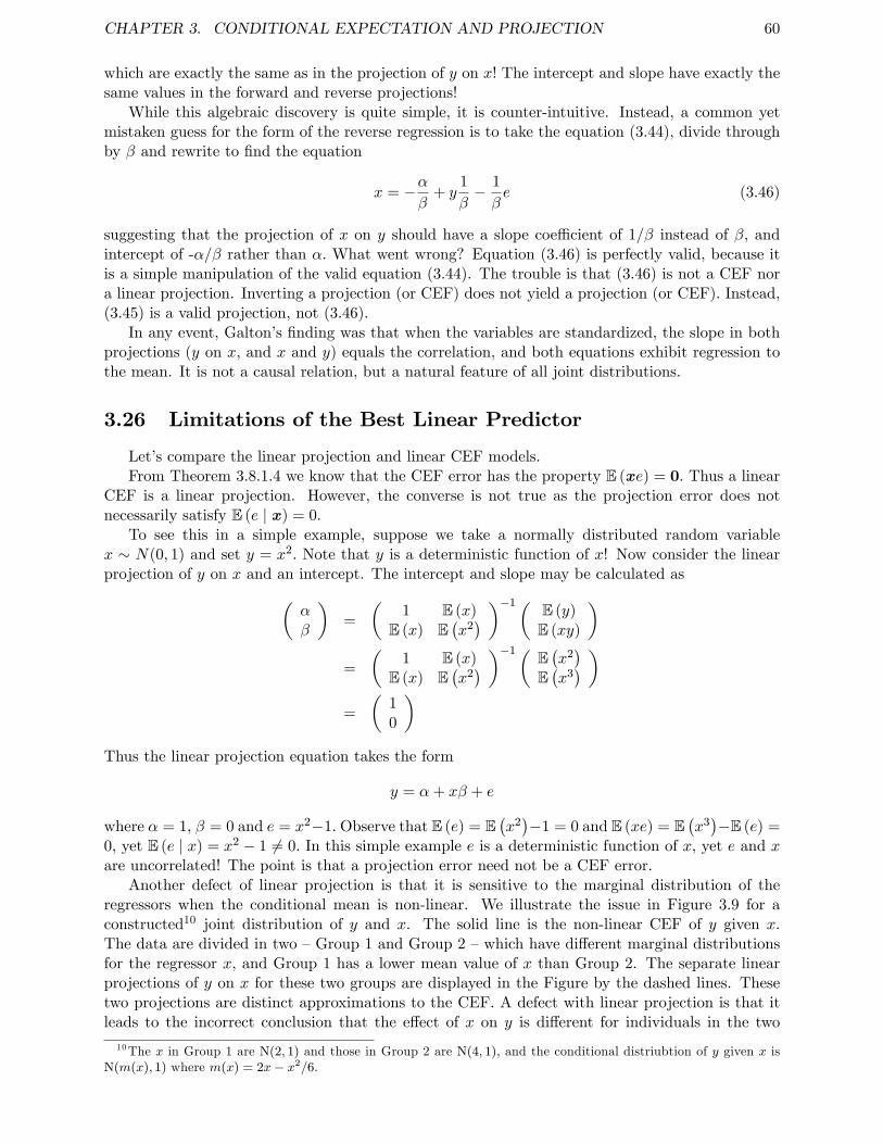
CHAPTER 3. CONDITIONAL EXPECTATION AND PROJECTION 60
which are exactly the same as in the projection of y on x! The intercept and slope have exactly thesame values in the forward and reverse projections!
While this algebraic discovery is quite simple, it is counter-intuitive. Instead, a common yetmistaken guess for the form of the reverse regression is to take the equation (3.44), divide throughby β and rewrite to find the equation
x = −αβ
+ y1
β− 1
βe (3.46)
suggesting that the projection of x on y should have a slope coeffi cient of 1/β instead of β, andintercept of -α/β rather than α. What went wrong? Equation (3.46) is perfectly valid, because itis a simple manipulation of the valid equation (3.44). The trouble is that (3.46) is not a CEF nora linear projection. Inverting a projection (or CEF) does not yield a projection (or CEF). Instead,(3.45) is a valid projection, not (3.46).
In any event, Galton’s finding was that when the variables are standardized, the slope in bothprojections (y on x, and x and y) equals the correlation, and both equations exhibit regression tothe mean. It is not a causal relation, but a natural feature of all joint distributions.
3.26 Limitations of the Best Linear Predictor
Let’s compare the linear projection and linear CEF models.From Theorem 3.8.1.4 we know that the CEF error has the property E (xe) = 0. Thus a linear
CEF is a linear projection. However, the converse is not true as the projection error does notnecessarily satisfy E (e | x) = 0.
To see this in a simple example, suppose we take a normally distributed random variablex ∼ N(0, 1) and set y = x2. Note that y is a deterministic function of x! Now consider the linearprojection of y on x and an intercept. The intercept and slope may be calculated as(
αβ
)=
(1 E (x)
E (x) E(x2) )−1( E (y)
E (xy)
)=
(1 E (x)
E (x) E(x2) )−1( E
(x2)
E(x3) )
=
(10
)Thus the linear projection equation takes the form
y = α+ xβ + e
where α = 1, β = 0 and e = x2−1. Observe that E (e) = E(x2)−1 = 0 and E (xe) = E
(x3)−E (e) =
0, yet E (e | x) = x2 − 1 6= 0. In this simple example e is a deterministic function of x, yet e and xare uncorrelated! The point is that a projection error need not be a CEF error.
Another defect of linear projection is that it is sensitive to the marginal distribution of theregressors when the conditional mean is non-linear. We illustrate the issue in Figure 3.9 for aconstructed10 joint distribution of y and x. The solid line is the non-linear CEF of y given x.The data are divided in two —Group 1 and Group 2 —which have different marginal distributionsfor the regressor x, and Group 1 has a lower mean value of x than Group 2. The separate linearprojections of y on x for these two groups are displayed in the Figure by the dashed lines. Thesetwo projections are distinct approximations to the CEF. A defect with linear projection is that itleads to the incorrect conclusion that the effect of x on y is different for individuals in the two
10The x in Group 1 are N(2, 1) and those in Group 2 are N(4, 1), and the conditional distriubtion of y given x isN(m(x), 1) where m(x) = 2x− x2/6.
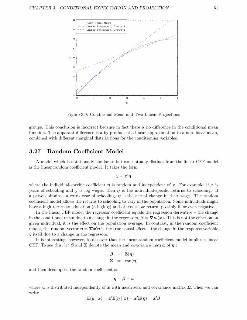
CHAPTER 3. CONDITIONAL EXPECTATION AND PROJECTION 61
Figure 3.9: Conditional Mean and Two Linear Projections
groups. This conclusion is incorrect because in fact there is no difference in the conditional meanfunction. The apparant difference is a by-product of a linear approximation to a non-linear mean,combined with different marginal distributions for the conditioning variables.
3.27 Random Coeffi cient Model
A model which is notationally similar to but conceptually distinct from the linear CEF modelis the linear random coeffi cient model. It takes the form
y = x′η
where the individual-specific coeffi cient η is random and independent of x. For example, if x isyears of schooling and y is log wages, then η is the individual-specific returns to schooling. Ifa person obtains an extra year of schooling, η is the actual change in their wage. The randomcoeffi cient model allows the returns to schooling to vary in the population. Some individuals mighthave a high return to education (a high η) and others a low return, possibly 0, or even negative.
In the linear CEF model the regressor coeffi cient equals the regression derivative —the changein the conditional mean due to a change in the regressors, β = ∇m(x). This is not the effect on angiven individual, it is the effect on the population average. In contrast, in the random coeffi cientmodel, the random vector η =∇x′η is the true causal effect —the change in the response variabley itself due to a change in the regressors.
It is interesting, however, to discover that the linear random coeffi cient model implies a linearCEF. To see this, let β and Σ denote the mean and covariance matrix of η :
β = E(η)
Σ = var (η)
and then decompose the random coeffi cient as
η = β + u
where u is distributed independently of x with mean zero and covariance matrix Σ. Then we canwrite
E(y | x) = x′E(η | x) = x′E(η) = x′β
CHAPTER 3. CONDITIONAL EXPECTATION AND PROJECTION 62
so the CEF is linear in x, and the coeffi cients β equal the mean of the random coeffi cient η.We can thus write the equation as a linear CEF
y = x′β + e (3.47)
where e = x′u and u = η − β. The error is conditionally mean zero:
E(e | x) = 0.
Furthermore
var (e | x) = x′ var (η)x
= x′Σx
so the error is conditionally heteroskedastic with its variance a quadratic function of x.
Theorem 3.27.1 In the linear random coeffi cient model y = x′η with η indepen-dent of x, E ‖x‖2 <∞, and E ‖η‖2 <∞, then
E (y | x) = x′β
var (y | x) = x′Σx
where β = E(η) and Σ = var (η).
3.28 Causal Effects
So far we have avoided the concept of causality, yet often the underlying goal of an econometricanalysis is to uncover a causal relationship between variables. It is often of great interest tounderstand the causes and effects of decisions, actions, and policies. For example, we may beinterested in the effect of class sizes on test scores, police expenditures on crime rates, climatechange on economic activity, years of schooling on wages, institutional structure on growth, theeffectiveness of rewards on behavior, the consequences of medical procedures for health outcomes,or any variety of possible causal relationships. In each case, the goal is to understand what is theactual effect on the outcome y due to a change in the input x. We are not just interested in theconditional mean or linear projection, we would like to know the actual change. The causal effectis typically specific to an individual, and also cannot be directly observed.
For example, the causal effect of schooling on wages is the actual difference a person would re-ceive in wages if we could change their level of education. The causal effect of a medical treatment isthe actual difference in an individual’s health outcome, comparing treatment versus non-treatment.In both cases the effects are individual and unobservable. For example, suppose that Jennifer wouldhave earned $10 an hour as a high-school graduate and $20 a hour as a college graduate while Georgewould have earned $8 as a high-school graduate and $12 as a college graduate. In this example thecausal effect of schooling is $10 a hour for Jennifer and $4 an hour for George. Furthermore, thecausal effect is unobserved as we only observe the wage corresponding to the actual outcome.
A variable x1 can be said to have a causal effect on the response variable y if the latter changeswhen all other inputs are held constant. To make this precise we need a mathematical formulation.We can write a full model for the response variable y as
y = h (x1,x2,u) (3.48)
CHAPTER 3. CONDITIONAL EXPECTATION AND PROJECTION 63
where x1 and x2 are the observed variables, u is an ` × 1 unobserved random factor, and h is afunctional relationship. This framework includes as a special case the random coeffi cient model(3.27) studied earlier. We define the causal effect of x1 within this model as the change in y due toa change in x1 holding the other variables x2 and u constant.
Definition 3.28.1 In the model (3.48) the the causal eff ect of x1 on y is
C(x1,x2,u) =∇1h (x1,x2,u) , (3.49)
the change in y due to a change in x1, holding x2 and u constant.
To understand this concept, imagine taking a single individual. As far as our structural model isconcerned, this person is described by their observables x1 and x2, and their unobservables u. In awage regression the unobservables would include characteristics such as the person’s abilities, skills,work ethic, interpersonal connections, and preferences. The causal effect of x1 (say, education) isthe change in the wage as x1 changes, holding constant all other observables and unobservables.
It may be helpful to understand that (3.49) is a definition, and does not necessarily describecausality in a fundamental or experimental sense. Perhaps it would be more appropriate to label(3.49) as a structural effect (the effect within the structural model).
Sometimes it is useful to write this relationship as a potential outcome function
y(x1) = h (x1,x2,u)
where the notation implies that y(x1) is holding x2 and u constant.A popular example arises in the analysis of treatment effects with a binary regressor x1. Let x1 =
1 indicate treatment (e.g. a medical procedure) and x1 = 0 indicating non-treatment. In this casey(x1) can be written
y(0) = h (0,x2,u)
y(1) = h (1,x2,u)
In the literature on treatment effects, it is common to refer to y(0) and y(1) as the latent outcomesassociated with non-treatment and treatment, respectively. That is, for a given individual, y(0) isthe health outcome if there is no treatment, and y(1) is the health outcome if there is treatment.The causal effect of treatment for the individual is the change in their health outcome due totreatment —the change in y as we hold both x2 and u constant:
C (x2,u) = y(1)− y(0).
This is random (a function of x2 and u) as both potential outcomes y(0) and y(1) are differentacross individuals.
In a sample, we cannot observe both outcomes from the same individual, we only observe therealized value
y =
y(0) if x1 = 0
y(1) if x1 = 1
As the causal effect varies across individuals and is not observable, it cannot be measured onthe individual level. We therefore focus on aggregate causal effects, in particular what is known asthe average causal effect.
CHAPTER 3. CONDITIONAL EXPECTATION AND PROJECTION 64
Definition 3.28.2 In the model (3.48) average causal eff ect of x1 on y condi-tional on x2 is
ACE(x1,x2) = E (C(x1,x2,u) | x1,x2) =
∫R`∇1h (x1,x2,u) f(u | x1,x2)du
(3.50)where f(u | x1,x2) is the conditional density of u given x1,x2.
We can think of the average causal effect ACE(x1,x2) as the average effect in the generalpopulation.
What is the relationship beteween the average causal effect ACE(x1,x2) and the regressionderivative ∇1m (x1,x2)? Equation (3.48) implies that the CEF is
m(x1,x2) = E (h (x1,x2,u) | x1,x2)
=
∫R`h (x1,x2,u) f(u | x1,x2)du,
the average causal equation, averaged over the conditional distribution of the observed componentu.
Applying the marginal effect operator, the regression derivative is
∇1m(x1,x2) =
∫R`∇1h (x1,x2,u) f(u | x1,x2)du+
∫R`h (x1,x2,u)∇1f(u | x1,x2)du
= ACE(x1,x2) +
∫R`h (x1,x2,u)∇1f(u | x1,x2)du. (3.51)
In general, the average causal effect is not the regression derivative. However, they equal whenthe second component in (3.51) is zero. This occurs when ∇1f(u | x1,x2) = 0, that is, whenthe conditional density of u given (x1,x2) does not depend on x1. The condition is suffi cientlyimportant that it has a special name in the treatment effects literature.
Definition 3.28.3 Conditional Independence Assumption (CIA). Condi-tional on x2, the random variables x1 and u are statistically independent.
The CIA implies f(u | x1,x2) = f(u | x2) does not depend on x1, and thus∇1f(u | x1,x2) = 0.Thus the CIA implies that∇1m(x1,x2) = ACE(x1,x2), the regression derivative equals the averagecausal effect.
Theorem 3.28.1 In the structural model (3.48), the Conditional Independence As-sumption implies
∇1m(x1,x2) = ACE(x1,x2)
the regression derivative equals the average causal effect for x1 on y conditional on x2.
This is a fascinating result. It shows that whenever the unobservable is independent of thetreatment variable (after conditioning on appropriate regressors) the regression derivative equals theaverage causal effect. In this case, the CEF has causal economic meaning, giving strong justification
CHAPTER 3. CONDITIONAL EXPECTATION AND PROJECTION 65
to estimation of the CEF. Our derivation also shows the critical role of the CIA. If CIA fails, thenthe equality of the regression derivative and ACE fails.
This theorem is quite general. It applies equally to the treatment-effects model where x1 isbinary or to more general settings where x1 is continuous.
It is also helpful to understand that the CIA is weaker than full independence of u from theregressors (x1,x2). The CIA was introduced precisely as a minimal suffi cient condition to obtainthe desired result. Full independence implies the CIA and implies that each regression derivativeequal that variable’s average causal effect, but full independence is not necessary in order to beable to causally interpret a subset of the regressors.
3.29 Existence and Uniqueness of the Conditional Expectation*
In Sections 3.3 and 3.5 we defined the conditional mean when the conditioning variables xare discrete and when the variables (y,x) have a joint density. We have explored these casesbecause these are the situations where the conditional mean is easiest to describe and understand.However, the conditional mean can be defined without appealing to the properties of either discreteor continuous random variables. The conditional mean exists quite generally.
To justify this claim we now present a deep result from probability theory. What is says is thatthe conditional mean exists for all joint distributions (y,x). The only requirement is that y has afinite mean.
Theorem 3.29.1 Existence of the Conditional MeanIf E |y| <∞ then there exists a function m(x) such that for all measurable sets X
E (1 (x ∈ X ) y) = E (1 (x ∈ X )m(x)) . (3.52)
The function m(x) is almost everywhere unique, in the sense that if h(x) satisfies(3.52), then there is a set S such that Pr(S) = 1 and m(x) = h(x) for x ∈ S. Thefunction m(x) is called the conditional mean and is written m(x) = E (y | x) .
See, for example, Ash (1972), Theorem 6.3.3.
The conditional meanm(x) defined by (3.52) specializes to (3.7) when (y,x) have a joint density.The usefulness of definition (3.52) is that Theorem 3.29.1 shows that the conditional mean m(x)exists for all finite-mean distributions. This definition allows y to be discrete or continuous, for x tobe scalar or vector-valued, and for the components of x to be discrete or continuously distributed.
Theorem 3.29.1 also demonstrates that E |y| <∞ is a suffi cient condition for identification of theconditional mean. (Recall, a parameter is identified if it is uniquely determined by the distributionof the observed variables.)
Theorem 3.29.2 Identification of the Conditional MeanIf E |y| <∞, the conditional mean m(x) = E (y | x) is identified almost everywhere.
CHAPTER 3. CONDITIONAL EXPECTATION AND PROJECTION 66
3.30 Technical Proofs*
Proof of Theorem 3.6.1:For convenience, assume that the variables have a joint density f (y,x). Since E (y | x) is a
function of the random vector x only, to calculate its expectation we integrate with respect to thedensity fx (x) of x, that is
E (E (y | x)) =
∫RkE (y | x) fx (x) dx.
Substituting in (3.7) and noting that fy|x (y|x) fx (x) = f (y,x) , we find that the above expressionequals ∫
Rk
(∫Ryfy|x (y|x) dy
)fx (x) dx =
∫Rk
∫Ryf (y,x) dydx = E (y)
the unconditional mean of y.
Proof of Theorem 3.6.2:Again assume that the variables have a joint density. It is useful to observe that
f (y|x1,x2) f (x2|x1) =f (y,x1,x2)
f (x1,x2)
f (x1,x2)
f (x1)= f (y,x2|x1) , (3.53)
the density of (y,x2) given x1. Here, we have abused notation and used a single symbol f to denotethe various unconditional and conditional densities to reduce notational clutter.
Note that
E (y | x1,x2) =
∫Ryf (y|x1,x2) dy. (3.54)
Integrating (3.54) with respect to the conditional density of x2 given x1, and applying (3.53) wefind that
E (E (y | x1,x2) | x1) =
∫Rk2
E (y | x1,x2) f (x2|x1) dx2
=
∫Rk2
(∫Ryf (y|x1,x2) dy
)f (x2|x1) dx2
=
∫Rk2
∫Ryf (y|x1,x2) f (x2|x1) dydx2
=
∫Rk2
∫Ryf (y,x2|x1) dydx2
= E (y | x1)
as stated.
Proof of Theorem 3.6.3:
E (g (x) y | x) =
∫Rg (x) yfy|x (y|x) dy = g (x)
∫Ryfy|x (y|x) dy = g (x)E (y | x)
This is (3.9). The assumption that E |g (x) y| < ∞ is required for the first equality to be well-defined. Equation (3.10) follows by applying the Simple Law of Iterated Expectations to (3.9).
Proof of Theorem 3.7.1: The assumption that Ey2 <∞ implies that all the conditional expec-tations below exist.
CHAPTER 3. CONDITIONAL EXPECTATION AND PROJECTION 67
Set z = E(y | x1,x2). By the conditional Jensen’s inequality (B.16),
(E(z | x1))2 ≤ E(z2 | x1
).
Taking unconditional expectations, this implies
E (E(y | x1))2 ≤ E(
(E(y | x1,x2))2).
Similarly,
(Ey)2 ≤ E(
(E(y | x1))2)≤ E
((E(y | x1,x2))2
). (3.55)
The variables y, E(y | x1) and E(y | x1,x2) all have the same mean Ey, so the inequality (3.55)implies that the variances are ranked monotonically:
0 ≤ var (E(y | x1)) ≤ var (E(y | x1,x2)) . (3.56)
Next, for µ = Ey observe that
E (y − E(y | x)) (E(y | x)− µ) = E (y − E(y | x)) (E(y | x)− µ) = 0
so the decompositiony − µ = y − E(y | x) + E(y | x)− µ
satisfiesvar (y) = var (y − E(y | x)) + var (E(y | x)) . (3.57)
The monotonicity of the variances of the conditional mean (3.56) applied to the variance decom-position (3.57) implies the reverse monotonicity of the variances of the differences, completing theproof.
Proof of Theorem 3.8.1. Applying Minkowski’s Inequality (B.22) to e = y −m(x),
(E |e|r)1/r = (E |y −m(x)|r)1/r ≤ (E |y|r)1/r + (E |m(x)|r)1/r <∞,
where the two parts on the right-hand are finite since E |y|r <∞ by assumption and E |m(x)|r <∞by the Conditional Expectation Inequality (B.17). The fact that (E |e|r)1/r < ∞ implies E |e|r <∞.
Proof of Theorem 3.16.1. For part 1, by the Expectation Inequality (B.18), (A.6) and Assump-tion 3.16.1, ∥∥E (xx′)∥∥ ≤ E∥∥xx′∥∥ = E ‖x‖2 <∞.Similarly, using the Expectation Inequality (B.18), the Cauchy-Schwarz Inequality (B.20) and As-sumption 3.16.1,
‖E (xy)‖ ≤ E ‖xy‖ =(E ‖x‖2
)1/2 (Ey2
)1/2<∞.
Thus the moments E (xy) and E (xx′) are finite and well defined.For part 2, the coeffi cient β = (E (xx′))−1 E (xy) is well defined since (E (xx′))−1 exists under
Assumption 3.16.1.Part 3 follows from Definition 3.16.1 and part 2.For part 4, first note that
Ee2 = E(y − x′β
)2= Ey2 − 2E
(yx′)β + β′E
(xx′)β
= Ey2 − 2E(yx′) (E(xx′))−1 E (xy)
≤ Ey2
< ∞
CHAPTER 3. CONDITIONAL EXPECTATION AND PROJECTION 68
The first inequality holds because E (yx′) (E (xx′))−1 E (xy) is a quadratic form and therefore neces-sarily non-negative. Second, by the Expectation Inequality (B.18), the Cauchy-Schwarz Inequality(B.20) and Assumption 3.16.1,
‖E (xe)‖ ≤ E ‖xe‖ =(E ‖x‖2
)1/2 (Ee2)1/2
<∞.
It follows that the expectation E (xe) is finite, and is zero by the calculation (3.26).For part 6, Applying Minkowski’s Inequality (B.22) to e = y − x′β,
(E |e|r)1/r =(E∣∣y − x′β∣∣r)1/r
≤ (E |y|r)1/r +(E∣∣x′β∣∣r)1/r
≤ (E |y|r)1/r + (E ‖x‖r)1/r ‖β‖< ∞,
the final inequality by assumption.
CHAPTER 3. CONDITIONAL EXPECTATION AND PROJECTION 69
Exercises
Exercise 3.1 Find E (E (E (y | x1,x2,x3) | x1,x2) | x1) .
Exercise 3.2 If E (y | x) = a+ bx, find E (yx) as a function of moments of x.
Exercise 3.3 Prove Theorem 3.8.1.4 using the law of iterated expectations.
Exercise 3.4 Suppose that the random variables y and x only take the values 0 and 1, and havethe following joint probability distribution
x = 0 x = 1
y = 0 .1 .2y = 1 .4 .3
Find E (y | x) , E(y2 | x
)and var (y | x) for x = 0 and x = 1.
Exercise 3.5 Show that σ2(x) is the best predictor of e2 given x:
(a) Write down the mean-squared error of a predictor h(x) for e2.
(b) What does it mean to be predicting e2?
(c) Show that σ2(x) minimizes the mean-squared error and is thus the best predictor.
Exercise 3.6 Use y = m(x) + e to show that
var (y) = var (m(x)) + σ2
Exercise 3.7 Show that the conditional variance can be written as
σ2(x) = E(y2 | x
)− (E (y | x))2 .
Exercise 3.8 Suppose that y is discrete-valued, taking values only on the non-negative integers,and the conditional distribution of y given x is Poisson:
Pr (y = j | x) =exp (−x′β) (x′β)j
j!, j = 0, 1, 2, ...
Compute E (y | x) and var (y | x) . Does this justify a linear regression model of the form y =x′β + e?
Hint: If Pr (y = j) = exp(−λ)λj
j! , then Ey = λ and var(y) = λ.
Exercise 3.9 Suppose you have two regressors: x1 is binary (takes values 0 and 1) and x2 iscategorical with 3 categories (A,B,C). Write E (y | x1, x2) as a linear regression.
Exercise 3.10 True or False. If y = xβ + e, x ∈ R, and E (e | x) = 0, then E(x2e)
= 0.
Exercise 3.11 True or False. If y = xβ + e, x ∈ R, and E (xe) = 0, then E(x2e)
= 0.
Exercise 3.12 True or False. If y = x′β + e and E (e | x) = 0, then e is independent of x.
Exercise 3.13 True or False. If y = x′β + e and E(xe) = 0, then E (e | x) = 0.
CHAPTER 3. CONDITIONAL EXPECTATION AND PROJECTION 70
Exercise 3.14 True or False. If y = x′β + e, E (e | x) = 0, and E(e2 | x
)= σ2, a constant, then
e is independent of x.
Exercise 3.15 Let x and y have the joint density f (x, y) = 32
(x2 + y2
)on 0 ≤ x ≤ 1, 0 ≤ y ≤ 1.
Compute the coeffi cients of the best linear predictor y = α+βx+e. Compute the conditional meanm(x) = E (y | x) . Are the best linear predictor and conditional mean different?
Exercise 3.16 Let x be a random variable with µ = Ex and σ2 = var(x). Define
g(x | µ, σ2
)=
(x− µ
(x− µ)2 − σ2
).
Show that Eg (x | m, s) = 0 if and only if m = µ and s = σ2.
Exercise 3.17 Suppose that
x =
1x2
x3
and x3 = α1 + α2x2 is a linear function of x2.
(a) Show that Qxx = E (xx′) is not invertible.
(b) Use a linear transformation of x to find an expression for the best linear predictor of y givenx. (Be explicit, do not just use the generalized inverse formula.)
Exercise 3.18 Show (3.42)-(3.43), namely that for
d(β) = E(m(x)− x′β
)2then
β = argminβ∈Rk
d(β)
=(E(xx′))−1 E (xm(x))
=(E(xx′))−1 E (xy) .
Hint: To show E (xm(x)) = E (xy) use the law of iterated expectations.
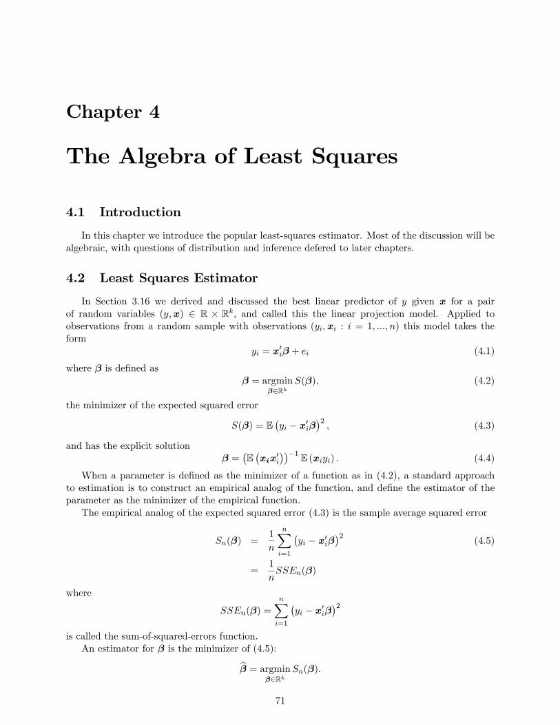
Chapter 4
The Algebra of Least Squares
4.1 Introduction
In this chapter we introduce the popular least-squares estimator. Most of the discussion will bealgebraic, with questions of distribution and inference defered to later chapters.
4.2 Least Squares Estimator
In Section 3.16 we derived and discussed the best linear predictor of y given x for a pairof random variables (y,x) ∈ R × Rk, and called this the linear projection model. Applied toobservations from a random sample with observations (yi,xi : i = 1, ..., n) this model takes theform
yi = x′iβ + ei (4.1)
where β is defined asβ = argmin
β∈RkS(β), (4.2)
the minimizer of the expected squared error
S(β) = E(yi − x′iβ
)2, (4.3)
and has the explicit solutionβ =
(E(xix
′i
))−1 E (xiyi) . (4.4)
When a parameter is defined as the minimizer of a function as in (4.2), a standard approachto estimation is to construct an empirical analog of the function, and define the estimator of theparameter as the minimizer of the empirical function.
The empirical analog of the expected squared error (4.3) is the sample average squared error
Sn(β) =1
n
n∑i=1
(yi − x′iβ
)2 (4.5)
=1
nSSEn(β)
where
SSEn(β) =
n∑i=1
(yi − x′iβ
)2is called the sum-of-squared-errors function.
An estimator for β is the minimizer of (4.5):
β = argminβ∈Rk
Sn(β).
71
CHAPTER 4. THE ALGEBRA OF LEAST SQUARES 72
Figure 4.1: Sum-of-Squared Errors Function
Alternatively, as Sn(β) is a scale multiple of SSEn(β), we may equivalently define β as the min-imizer of SSEn(β). Hence β is commonly called the least-squares (LS) (or ordinary leastsquares (OLS)) estimator of β. As discussed in Chapter 2, the hat “^”on β signifies that it isan estimator of the parameter β. If we want to be explicit about the estimation method, we canwrite βols to signify that it is the OLS estimator.
To visualize the quadratic function Sn(β), Figure 4.1 displays an example sum-of-squared er-rors function SSEn(β) for the case k = 2. The least-squares estimator β is the the pair (β1, β2)minimizing this function.
4.3 Solving for Least Squares
To solve for β, expand the SSE function to find
SSEn(β) =
n∑i=1
y2i − 2β′
n∑i=1
xiyi + β′n∑i=1
xix′iβ
which is quadratic in the vector argument β . The first-order-condition for minimization of SSEn(β)is
0 =∂
∂βSSEn(β) = −2
n∑i=1
xiyi + 2
n∑i=1
xix′iβ. (4.6)
By inverting the k×k matrix∑n
i=1 xix′i we find an explicit formula for the least-squares estimator
β =
(n∑i=1
xix′i
)−1( n∑i=1
xiyi
). (4.7)
This is the natural estimator of the best linear projection coeffi cient β defined in (4.2), and canalso be called the linear projection estimator.
CHAPTER 4. THE ALGEBRA OF LEAST SQUARES 73
Alternatively, equation (4.4) writes the projection coeffi cient β as an explicit function of thepopulation moments Qxy and Qxx. Their moment estimators are the sample moments
Qxy =1
n
n∑i=1
xiyi
Qxx =1
n
n∑i=1
xix′i.
The moment estimator of β replaces the population moments in (4.4) with the sample moments:
β = Q−1
xx Qxy
=
(1
n
n∑i=1
xix′i
)−1(1
n
n∑i=1
xiyi
)
=
(n∑i=1
xix′i
)−1( n∑i=1
xiyi
)which is identical with (4.7).
Least Squares Estimation
Definition 4.3.1 The least-squares estimator β is
β = argminβ∈Rk
Sn(β)
where
Sn(β) =1
n
n∑i=1
(yi − x′iβ
)2and has the solution
β =
(n∑i=1
xix′i
)−1( n∑i=1
xiyi
).
Adrien-Marie Legendre
The method of least-squares was first published in 1805 by the French mathematicianAdrien-Marie Legendre (1752-1833). Legendre proposed least-squares as a solution to thealgebraic problem of solving a system of equations when the number of equations exceededthe number of unknowns. This was a vexing and common problem in astronomical mea-surement. As viewed by Legendre, (4.1) is a set of n equations with k unknowns. As theequations cannot be solved exactly, Legendre’s goal was to select β to make the set oferrors as small as possible. He proposed the sum of squared error criterion, and derivedthe algebraic solution presented above. As he noted, the first-order conditions (4.6) is asystem of k equations with k unknowns, which can be solved by “ordinary”methods. Hencethe method became known as Ordinary Least Squares and to this day we still use theabbreviation OLS to refer to Legendre’s estimation method.
CHAPTER 4. THE ALGEBRA OF LEAST SQUARES 74
4.4 Illustration
We illustrate the least-squares estimator in practice with the data set used to generate theestimates from Chapter 3. This is the March 2009 Current Population Survey, which has extensiveinformation on the U.S. population. This data set is described in more detail in Section ? For thisillustration, we use the sub-sample of non-white married non-military female wages earners with12 years potential work experience. This sub-sample has 61 observations. Let yi be log wages andxi be an intercept and years of education. Then
1
n
n∑i=1
xiyi =
(3.02547.447
)and
1
n
n∑i=1
xix′i =
(1 15.426
15.426 243
).
Thus
β =
(1 15.426
15.426 243
)−1(3.02547.447
)
=
(0.6260.156
). (4.8)
We often write the estimated equation using the format
log(Wage) = 0.626 + 0.156 education. (4.9)
An interpretation of the estimated equation is that each year of education is associated with an16% increase in mean wages.
Equation (4.9) is called a bivariate regression as there are only two variables. A multivari-ate regression has two or more regressors, and allows a more detailed investigation. Let’s redothe example, but now including all levels of experience. This expanded sample includes 2454 ob-servations. Including as regressors years of experience and its square (experience2/100) (we divideby 100 to simplify reporting), we obtain the estimates
log(Wage) = 1.06 + 0.116 education+ 0.010 experience− 0.014 experience2/100. (4.10)
These estimates suggest a 12% increase in mean wages per year of education, holding experienceconstant.
4.5 Least Squares Residuals
As a by-product of estimation, we define the fitted or predicted value
yi = x′iβ
and the residualei = yi − yi = yi − x′iβ. (4.11)
Note that yi = yi + ei andyi = x′iβ + ei. (4.12)
We make a distinction between the error ei and the residual ei. The error ei is unobservable whilethe residual ei is a by-product of estimation. These two variables are frequently mislabeled, whichcan cause confusion.
CHAPTER 4. THE ALGEBRA OF LEAST SQUARES 75
Equation (4.6) implies thatn∑i=1
xiei = 0. (4.13)
To see this by a direct calculation, using (4.11) and (4.7),
n∑i=1
xiei =
n∑i=1
xi
(yi − x′iβ
)=
n∑i=1
xiyi −n∑i=1
xix′iβ
=n∑i=1
xiyi −n∑i=1
xix′i
(n∑i=1
xix′i
)−1( n∑i=1
xiyi
)
=n∑i=1
xiyi −n∑i=1
xiyi
= 0.
When xi contains a constant, an implication of (4.13) is
1
n
n∑i=1
ei = 0.
Thus the residuals have a sample mean of zero and the sample correlation between the regressorsand the residual is zero. These are algebraic results, and hold true for all linear regression estimates.
Given the residuals, we can construct an estimator for σ2 = Ee2i :
σ2 =1
n
n∑i=1
e2i . (4.14)
4.6 Model in Matrix Notation
For many purposes, including computation, it is convenient to write the model and statistics inmatrix notation. The linear equation (3.24) is a system of n equations, one for each observation.We can stack these n equations together as
y1 = x′1β + e1
y2 = x′2β + e2
...
yn = x′nβ + en.
Now define
y =
y1
y2...yn
, X =
x′1x′2...x′n
, e =
e1
e2...en
.
Observe that y and e are n× 1 vectors, and X is an n× k matrix. Then the system of n equationscan be compactly written in the single equation
y = Xβ + e. (4.15)
CHAPTER 4. THE ALGEBRA OF LEAST SQUARES 76
Sample sums can also be written in matrix notation. For example
n∑i=1
xix′i = X ′X
n∑i=1
xiyi = X ′y.
Thereforeβ =
(X ′X
)−1 (X ′y
). (4.16)
The matrix version of (4.12) and estimated version of (4.15) is
y = Xβ + e,
or equivalently the residual vector ise = y −Xβ.
Using the residual vector, we can write (4.13) as
X ′e = 0 (4.18)
and the error variance estimator (4.14) as
σ2 = n−1e′e (4.19)
Using matrix notation we have simple expressions for most estimators. This is particularlyconvenient for computer programming, as most languages allow matrix notation and manipulation.
Important Matrix Expressions
y = Xβ + e
β =(X ′X
)−1 (X ′y
)e = y −Xβ
X ′e = 0
σ2 = n−1e′e.
Early Use of Matrices
The earliest known treatment of the use of matrix methodsto solve simultaneous systems is found in Chapter 8 of theChinese text The Nine Chapters on the Mathematical Art,written by several generations of scholars from the 10th to2nd century BCE.
CHAPTER 4. THE ALGEBRA OF LEAST SQUARES 77
4.7 Projection Matrix
Define the matrixP = X
(X ′X
)−1X ′.
Observe thatPX = X
(X ′X
)−1X ′X = X.
This is a property of a projection matrix. More generally, for any matrix Z which can be writtenas Z = XΓ for some matrix Γ (we say that Z lies in the range space of X), then
PZ = PXΓ = X(X ′X
)−1X ′XΓ = XΓ = Z.
As an important example, if we partition the matrix X into two matrices X1 and X2 so that
X = [X1 X2] ,
then PX1 = X1.The matrix P is symmetric and idempotent1. To see that it is symmetric,
P ′ =(X(X ′X
)−1X ′)′
=(X ′)′ ((
X ′X)−1)′
(X)′
= X((X ′X
)′)−1X ′
= X(
(X)′(X ′)′)−1
X ′
= P .
To establish that it is idempotent, the fact that PX = X implies that
PP = PX(X ′X
)−1X ′
= X(X ′X
)−1X ′
= P .
The matrix P has the property that it creates the fitted values in a least-squares regression:
Py = X(X ′X
)−1X ′y = Xβ = y.
Because of this property, P is also known as the “hat matrix”.Another useful property is that the trace of P equals the number of columns of X
trP = k. (4.20)
Indeed,
trP = tr(X(X ′X
)−1X ′)
= tr((X ′X
)−1X ′X
)= tr (Ik)
= k.
1A matrix P is symmetric if P ′ = P . A matrix P is idempotent if PP = P . See Appendix A.8.
CHAPTER 4. THE ALGEBRA OF LEAST SQUARES 78
(See Appendix A.4 for definition and properties of the trace operator.)The i’th diagonal element of P = X (X ′X)
−1X ′ is
hii = x′i(X ′X
)−1xi (4.21)
which is called the leverage of the i’th observation. The hii take values in [0, 1] and sum to kn∑i=1
hii = k (4.22)
(See Exercise 4.8).
4.8 Orthogonal Projection
Define
M = In − P= In −X
(X ′X
)−1X ′
where In is the n× n identity matrix. Note that
MX = (In − P )X = X − PX = X −X = 0.
ThusM andX are orthogonal. We callM an orthogonal projection matrix or an annihilatormatrix due to the property that for any matrix Z in the range space of X then
MZ = Z − PZ = 0.
For example,MX1 = 0 for any subcomponent X1 of X, andMP = 0.The orthogonal projection matrixM has many similar properties with P , including thatM is
symmetric (M ′ = M) and idempotent (MM = M). Similarly to (4.20) we can calculate
trM = n− k. (4.23)
While P creates fitted values,M creates least-squares residuals:
My = y − Py = y −Xβ = e. (4.24)
Another way of writing (4.24) is
y = Py +My = y + e.
This decomposition is orthogonal, that is
y′e = (Py)′ (My) = y′PMy = 0.
We can also use (4.24) to write an alternative expression for the residual vector. Substitutingy = Xβ + e into e = My and usingMX = 0 we find
e = M (Xβ + e) = Me. (4.25)
which is free of dependence on the regression coeffi cient β.Another useful application of (4.24) is to the error variance estimator (4.19)
σ2 = n−1e′e
= n−1y′MMy
= n−1y′My,
the final equality sinceMM = M . Similarly using (4.25) we find
σ2 = n−1e′Me.
CHAPTER 4. THE ALGEBRA OF LEAST SQUARES 79
4.9 Regression Components
PartitionX = [X1 X2]
and
β =
(β1
β2
).
Then the regression model can be rewritten as
y = X1β1 +X2β2 + e. (4.26)
The OLS estimator of β = (β′1,β′2)′ is obtained by regression of y on X = [X1 X2] and can be
written asy = Xβ + e = X1β1 +X2β2 + e. (4.27)
We are interested in algebraic expressions for β1 and β2.The algebra for the estimator is identical as that for the population coeffi cients as presented in
Section 3.19.Partition Qxx and Qxy as
Qxx =
Q11 Q12
Q21 Q22
=
1
nX ′1X1
1
nX ′1X2
1
nX ′2X1
1
nX ′2X2
and similarly Qxy
Qxy =
Q1y
Q2y
=
1
nX ′1y
1
nX ′2y
.By the partitioned matrix inversion formula (A.4)
Q−1
xx =
Q11 Q12
Q21 Q22
−1
def=
Q11
Q12
Q21
Q22
=
Q−1
11·2 −Q−1
11·2Q12Q−1
22
−Q−1
22·1Q21Q−111 Q
−1
22·1
(4.28)
where Q11·2 = Q11 − Q12Q−1
22 Q21 and Q22·1 = Q22 − Q21Q−1
11 Q12.Thus
β =
(β1
β2
)
=
[Q−1
11·2 −Q−1
11·2Q12Q−1
22
−Q−1
22·1Q21Q−1
11 Q−1
22·1
][Q1y
Q2y
]
=
(Q−1
11·2Q1y·2
Q−1
22·1Q2y·1
)Now
Q11·2 = Q11 − Q12Q−1
22 Q21
=1
nX ′1X1 −
1
nX ′1X2
(1
nX ′2X2
)−1 1
nX ′2X1
=1
nX ′1M2X1
CHAPTER 4. THE ALGEBRA OF LEAST SQUARES 80
whereM2 = In −X2
(X ′2X2
)−1X ′2
is the orthogonal projection matrix for X2. Similarly Q22·1 =1
nX ′2M1X2 where
M1 = In −X1
(X ′1X1
)−1X ′1
is the orthogonal projection matrix for X1. Also
Q1y·2 = Q1y − Q12Q−1
22 Q2y
=1
nX ′1y −
1
nX ′1X2
(1
nX ′2X2
)−1 1
nX ′2y
=1
nX ′1M2y
and Q2y·1 =1
nX ′2M1y.
Thereforeβ1 =
(X ′1M2X1
)−1 (X ′1M2y
)(4.29)
andβ2 =
(X ′2M1X2
)−1 (X ′2M1y
). (4.30)
These are algebraic expressions for the sub-coeffi cient estimates from (4.27).
4.10 Residual Regression
As first recognized by Ragnar Frisch, expressions (4.29) and (4.30) can be used to show thatthe least-squares estimators β1 and β2 can be found by a two-step regression procedure.
Take (4.30). SinceM1 is idempotent,M1 = M1M1 and thus
β2 =(X ′2M1X2
)−1 (X ′2M1y
)=
(X ′2M1M1X2
)−1 (X ′2M1M1y
)=
(X′2X2
)−1 (X′2e1
)where
X2 = M1X2
ande1 = M1y.
Thus the coeffi cient estimate β2 is algebraically equal to the least-squares regression of e1 onX2. Notice that these two are y and X2, respectively, premultiplied by M1. But we know thatmultiplication by M1 is equivalent to creating least-squares residuals. Therefore e1 is simply theleast-squares residual from a regression of y on X1, and the columns of X2 are the least-squaresresiduals from the regressions of the columns of X2 on X1.
We have proven the following theorem.
CHAPTER 4. THE ALGEBRA OF LEAST SQUARES 81
Theorem 4.10.1 Frisch-Waugh-LovellIn the model (4.26), the OLS estimator of β2 and the OLS residuals emay be equivalently computed by either the OLS regression (4.27) or viathe following algorithm:
1. Regress y on X1, obtain residuals e1;
2. Regress X2 on X1, obtain residuals X2;
3. Regress e1 on X2, obtain OLS estimates β2 and residuals e.
In some contexts, the FWL theorem can be used to speed computation, but in most casesthere is little computational advantage to using the two-step algorithm. Rather, the primary useis theoretical.
A common application of the FWL theorem, which you may have seen in an introductoryeconometrics course, is the demeaning formula for regression. Partition X = [X1 X2] where X1
is the vector of observed regressors and X2 = ι is a vector of ones . In this case,
M2 = I − ι(ι′ι)−1
ι′.
Observe that
X1 = M2X1
= X1 − ι(ι′ι)−1
ι′X1
= X1 −X1
and
y = M2y
= y − ι(ι′ι)−1
ι′y
= y − y,
which are “demeaned”. The FWL theorem says that β1 is the OLS estimate from a regression ofyi − y on x1i − x1 :
β1 =
(n∑i=1
(x1i − x1) (x1i − x1)′)−1( n∑
i=1
(x1i − x1) (yi − y)
).
Thus the OLS estimator for the slope coeffi cients is a regression with demeaned data.
Ragnar Frisch
Ragnar Frisch (1895-1973) was co-winner with Jan Tinbergen of the first Nobel MemorialPrize in Economic Sciences in 1969 for their work in developing and applying dynamic mod-els for the analysis of economic problems. Frisch made a number of foundational contribu-tions to modern economics beyond the Frisch-Waugh-Lovell Theorem, including formalizingconsumer theory, production theory, and business cycle theory.
CHAPTER 4. THE ALGEBRA OF LEAST SQUARES 82
4.11 Prediction Errors
The least-squares residual ei are not true prediction errors, as they are constructed based onthe full sample including yi. A proper prediction for yi should be based on estimates constructedonly using the other observations. We can do this by defining the leave-one-out OLS estimatorof β as that obtained from the sample of n− 1 observations excluding the i’th observation:
β(−i) =
1
n− 1
∑j 6=ixjx
′j
−1 1
n− 1
∑j 6=ixjyj
=
(X ′(−i)X(−i)
)−1X(−i)y(−i). (4.31)
Here, X(−i) and y(−i) are the data matrices omitting the i’th row. The leave-one-out predictedvalue for yi is
yi = x′iβ(−i),
and the leave-one-out residual or prediction error is
ei = yi − yi.
A convenient alternative expression for β(−i) (derived below) is
β(−i) = β − (1− hii)−1 (X ′X)−1xiei (4.32)
where hii are the leverage values as defined in (4.21).Using (4.32) we can simplify the expression for the prediction error:
ei = yi − x′iβ(−i)
= yi − x′iβ + (1− hii)−1 x′i(X ′X
)−1xiei
= ei + (1− hii)−1 hiiei
= (1− hii)−1 ei. (4.33)
A convenient feature of this expression is that it shows that computation of ei is based on a simplelinear operation, and does not really require n separate estimations.
One use of the prediction errors is to estimate the out-of-sample mean squared error
σ2 =1
n
n∑i=1
e2i
=1
n
n∑i=1
(1− hii)−2 e2i .
This is also known as the mean squared prediction error. Its square root σ =√σ2 is the
prediction standard error.
Proof of Equation (4.32). The Sherman—Morrison formula (A.3) from Appendix A.5 states thatfor nonsingular A and vector b(
A− bb′)−1
= A−1 +(1− b′A−1b
)−1A−1bb′A−1.
This implies (X ′X − xix′i
)−1=(X ′X
)−1+ (1− hii)−1 (X ′X)−1
xix′i
(X ′X
)−1
CHAPTER 4. THE ALGEBRA OF LEAST SQUARES 83
and thus
β(−i) =(X ′X − xix′i
)−1 (X ′y − xiyi
)=
(X ′X
)−1X ′y −
(X ′X
)−1xiyi
+ (1− hii)−1 (X ′X)−1xix
′i
(X ′X
)−1 (X ′y − xiyi
)= β −
(X ′X
)−1xiyi + (1− hii)−1 (X ′X)−1
xi
(x′iβ − hiiyi
)= β − (1− hii)−1 (X ′X)−1
xi
((1− hii) yi − x′iβ + hiiyi
)= β − (1− hii)−1 (X ′X)−1
xiei
the third equality making the substitutions β = (X ′X)−1X ′y and hii = x′i (X ′X)
−1xi, and the
remainder collecting terms.
4.12 Influential Observations
Another use of the leave-one-out estimator is to investigate the impact of influential obser-vations, sometimes called outliers. We say that observation i is influential if its omission fromthe sample induces a substantial change in a parameter of interest. From (4.32)-(4.33) we knowthat
β − β(−i) = (1− hii)−1 (X ′X)−1xiei
=(X ′X
)−1xiei. (4.34)
By direct calculation of this quantity for each observation i, we can directly discover if a specificobservation i is influential for a coeffi cient estimate of interest.
For a general assessment, we can focus on the predicted values. The difference between thefull-sample and leave-one-out predicted values is
yi − yi = x′iβ − x′iβ(−i)
= x′i(X ′X
)−1xiei
= hiiei
which is a simple function of the leverage values hii and prediction errors ei. Observation i isinfluential for the predicted value if |hiiei| is large, which requires that both hii and |ei| are large.
One way to think about this is that a large leverage value hii gives the potential for observationi to be influential. A large hii means that observation i is unusual in the sense that the regressor xiis far from its sample mean. We call an observation with large hii a leverage point. A leveragepoint is not necessarily influential as the latter also requires that the prediction error ei is large.
To determine if any individual observations are influential in this sense, a large number ofdiagnostic statistics have been proposed (some names include DFITS, Cook’s Distance, and WelschDistance) but as they are not based on statistical theory it is unclear if they are useful for practicalwork. Probably the most relevant measure is the change in the coeffi cient estimates given in(4.34). The ratio of these changes to the coeffi cient’s standard error is called its DFBETA, and isa postestimation diagnostic available in STATA. While there is no magic threshold, the concern iswhether or not an individual observation meaningfully changes an estimated coeffi cient of interest.
For illustration, consider Figure 4.2 which shows a scatter plot of random variables (yi, xi).The 25 observations shown with the open circles are generated by xi ∼ U [1, 10] and yi ∼ N(xi, 4).The 26’th observation shown with the filled circle is x26 = 9, y26 = 0. (Imagine that y26 = 0 wasincorrectly recorded due to a mistaken key entry.) The Figure shows both the least-squares fitted
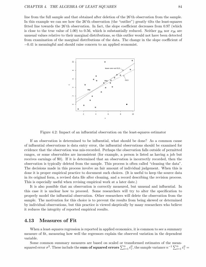
CHAPTER 4. THE ALGEBRA OF LEAST SQUARES 84
line from the full sample and that obtained after deletion of the 26’th observation from the sample.In this example we can see how the 26’th observation (the “outlier”) greatly tilts the least-squaresfitted line towards the 26’th observation. In fact, the slope coeffi cient decreases from 0.97 (whichis close to the true value of 1.00) to 0.56, which is substantially reduced. Neither y26 nor x26 areunusual values relative to their marginal distributions, so this outlier would not have been detectedfrom examination of the marginal distributions of the data. The change in the slope coeffi cient of−0.41 is meaningful and should raise concern to an applied economist.
2 4 6 8 10
02
46
810
x
y
leave−one−out OLS
OLS
Figure 4.2: Impact of an influential observation on the least-squares estimator
If an observation is determined to be influential, what should be done? As a common causeof influential observations is data entry error, the influential observations should be examined forevidence that the observation was mis-recorded. Perhaps the observation falls outside of permittedranges, or some observables are inconsistent (for example, a person is listed as having a job butreceives earnings of $0). If it is determined that an observation is incorrectly recorded, then theobservation is typically deleted from the sample. This process is often called “cleaning the data”.The decisions made in this process involve an fair amount of individual judgement. When this isdone it is proper empirical practice to document such choices. (It is useful to keep the source datain its original form, a revised data file after cleaning, and a record describing the revision process.This is especially useful when revising empirical work at a later date.)
It is also possible that an observation is correctly measured, but unusual and influential. Inthis case it is unclear how to proceed. Some researchers will try to alter the specification toproperly model the influential observation. Other researchers will delete the observation from thesample. The motivation for this choice is to prevent the results from being skewed or determinedby individual observations, but this practice is viewed skeptically by many researchers who believeit reduces the integrity of reported empirical results.
4.13 Measures of Fit
When a least-squares regression is reported in applied economics, it is common to see a summarymeasure of fit, measuring how well the regressors explain the observed variation in the dependentvariable.
Some common summary measures are based on scaled or transformed estimates of the mean-squared error σ2. These include the sum of squared errors
∑ni=1 e
2i , the sample variance n
−1∑n
i=1 e2i =
CHAPTER 4. THE ALGEBRA OF LEAST SQUARES 85
σ2, the root mean squared error√n−1
∑ni=1 e
2i (sometimes called the standard error of the re-
gression), and the mean prediction error σ2 = 1n
∑ni=1 e
2i .
A related and commonly reported statistic is the coeffi cient of determination orR-squared:
R2 =
∑ni=1 (yi − y)2∑ni=1 (yi − y)2 = 1− σ2
σ2y
where
σ2y =
1
n
n∑i=1
(yi − y)2
is the sample variance of yi. R2 can be viewed as an estimator of the population parameter
ρ2 =var (x′iβ)
var(yi)= 1− σ2
σ2y
where σ2y = var(yi). A high ρ2 means that forecasts of y using x′β will be quite accurate relative to
the unconditional mean. In this sense R2 can be a useful summary measure for an out-of-sampleforecast or policy experiment.
An alternative estimator of ρ2 proposed by Theil called R-bar-squared or adjusted R2 is
R2
= 1− (n− 1)∑n
i=1 e2i
(n− k)∑n
i=1 (yi − y)2 .
Theil’s estimator R2is better estimator of ρ2 than the unadjusted estimator R2 because it is a
ratio of bias-corrected variance estimates.Unfortunately, the frequent reporting of R2 and R
2seems to have led to exaggerated beliefs
regarding their usefulness. One mistaken belief is that R2 is a measure of “fit”. This belief isincorrect, as an incorrectly specified model can still have a reasonably high R2. For example,suppose the truth is that xi ∼ N(0, 1) and yi = βxi+x2
i . If we regress yi on xi (incorrectly omittingx2i ), the best linear predictor is yi = 1+βxi+ei where ei = x2
i −1. This is a misspecified regression,as the true relationship is deterministic! You can also calculate that the population ρ2 = β/(2 +β)which can be arbitrarily close to 1 if β is large. For example, if β = 8, then R2 ' ρ2 = .8, or ifβ = 18 then R2 ' ρ2 = .9. This example shows that a regression with a high R2 can actually havepoor fit.
Another mistaken belief is that a high R2 is important in order to justify interpretation of theregression coeffi cients. This is mistaken as there is no direct association between the level of R2
and the “correctness” of a regression, the accuracy of the coeffi cient estimates, or the validity ofstatistical inferences based on the estimated regression. In contrast, even if the R2 is quite small,accurate estimates of regression coeffi cients is quite possible when sample sizes are large.
The bottom line is that while R2 and R2have appropriate uses, their usefulness should not be
exaggerated.
Henri Theil
Henri Theil (1924-2000) of Holland invented R2and two-stage least squares, both of which
are routinely seen in applied econometrics. He also wrote an early and influential advancedtextbook on econometrics (Theil, 1971).
CHAPTER 4. THE ALGEBRA OF LEAST SQUARES 86
4.14 Normal Regression Model
The normal regression model is the linear regression model under the restriction that the errorei is independent of xi and has the distribution N
(0, σ2
). We can write this as
ei | xi ∼ N(0, σ2
).
This assumption impliesyi | xi ∼ N
(x′iβ, σ
2).
Normal regression is a parametric model, where likelihood methods can be used for estimation,testing, and distribution theory.
The log-likelihood function for the normal regression model is
logL(β, σ2) =
n∑i=1
log
(1
(2πσ2)1/2exp
(− 1
2σ2
(yi − x′iβ
)2))
= −n2
log(2πσ2
)− 1
2σ2SSEn(β).
The maximum likelihood estimator (MLE) (βmle, σ2mle) maximizes logL(β, σ2). Since the latter is
a function of β only through the sum of squared errors SSEn(β), maximizing the likelihood isidentical to minimizing SSEn(β). Hence
βmle = βols,
the MLE for β equals the OLS estimator. Due to this equivalence, the least squares estimator βols
is often called the MLE.We can also find the MLE for σ2. Plugging β into the log-likelihood we obtain
logL(β, σ2
)= −n
2log(2πσ2
)− 1
2σ2
n∑i=1
e2i .
Maximization with respect to σ2 yields the first-order condition
∂
∂σ2logL
(β, σ2
)= − n
2σ2 +1
2(σ2)2 n∑
i=1
e2i = 0.
Solving for σ2 yields the MLE for σ2
σ2mle =
1
n
n∑i=1
e2i
which is the same as the moment estimator (4.14).It may seem surprising that the MLE βmle is numerically equal to the OLS estimator, despite
emerging from quite different motivations. It is not completely accidental. The least-squaresestimator minimizes a particular sample loss function —the sum of squared error criterion —andmost loss functions are equivalent to the likelihood of a specific parametric distribution, in this casethe normal regression model. In this sense it is not surprising that the least-squares estimator canbe motivated as either the minimizer of a sample loss function or as the maximizer of a likelihoodfunction.

CHAPTER 4. THE ALGEBRA OF LEAST SQUARES 87
Carl Friedrich Gauss
The mathematician Carl Friedrich Gauss (1777-1855) proposed the normal regression model,and derived the least squares estimator as the maximum likelihood estimator for this model.He claimed to have discovered the method in 1795 at the age of eighteen, but did not publishthe result until 1809. Interest in Gauss’s approach was reinforced by Laplace’s simultaneousdiscovery of the central limit theorem, which provided a justification for viewing randomdisturbances as approximately normal.
CHAPTER 4. THE ALGEBRA OF LEAST SQUARES 88
Exercises
Exercise 4.1 Let y be a random variable with µ = Ey and σ2 = var(y). Define
g(y, µ, σ2
)=
(y − µ
(y − µ)2 − σ2
).
Let (µ, σ2) be the values such that gn(µ, σ2) = 0 where gn(m, s) = n−1∑n
i=1 g (yi,m, s) . Show thatµ and σ2 are the sample mean and variance.
Exercise 4.2 Consider the OLS regression of the n× 1 vector y on the n× k matrix X. Consideran alternative set of regressors Z = XC, where C is a k × k non-singular matrix. Thus, eachcolumn of Z is a mixture of some of the columns of X. Compare the OLS estimates and residualsfrom the regression of y on X to the OLS estimates from the regression of y on Z.
Exercise 4.3 Using matrix algebra, show X ′e = 0.
Exercise 4.4 Let e be the OLS residual from a regression of y on X = [X1 X2]. Find X ′2e.
Exercise 4.5 Let e be the OLS residual from a regression of y on X. Find the OLS coeffi cientfrom a regression of e on X.
Exercise 4.6 Let y = X(X ′X)−1X ′y. Find the OLS coeffi cient from a regression of y on X.
Exercise 4.7 Show that if X = [X1 X2] then PX1 = X1.
Exercise 4.8 Show (4.22), that hii in (4.21) sum to k. (Hint: Use (4.20).)
Exercise 4.9 Show thatM is idempotent: MM = M .
Exercise 4.10 Show that trM = n− k.
Exercise 4.11 Show that if X = [X1 X2] and X ′1X2 = 0 then P = P 1 + P 2.
Exercise 4.12 A dummy variable takes on only the values 0 and 1. It is used for categoricaldata, such as an individual’s gender. Let d1 and d2 be vectors of 1’s and 0’s, with the i′th elementof d1 equaling 1 and that of d2 equaling 0 if the person is a man, and the reverse if the person is awoman. Suppose that there are n1 men and n2 women in the sample. Consider fitting the followingthree equations by OLS
y = µ+ d1α1 + d2α2 + e (4.35)
y = d1α1 + d2α2 + e (4.36)
y = µ+ d1φ+ e (4.37)
Can all three equations (4.35), (4.36), and (4.37) be estimated by OLS? Explain if not.
(a) Compare regressions (4.36) and (4.37). Is one more general than the other? Explain therelationship between the parameters in (4.36) and (4.37).
(b) Compute ι′d1 and ι′d2, where ι is an n× 1 is a vector of ones.
(c) Letting α = (α1 α2)′, write equation (4.36) as y = Xα + e. Consider the assumptionE(xiei) = 0. Is there any content to this assumption in this setting?
CHAPTER 4. THE ALGEBRA OF LEAST SQUARES 89
Exercise 4.13 Let d1 and d2 be defined as in the previous exercise.
(a) In the OLS regressiony = d1γ1 + d2γ2 + u,
show that γ1 is the sample mean of the dependent variable among the men of the sample(y1), and that γ2 is the sample mean among the women (y2).
(b) Let X (n× k) be an additional matrix of regressions. Describe in words the transformations
y∗ = y − d1y1 − d2y2
X∗ = X − d1X1 − d2X2.
(c) Compare β from the OLS regresion
y∗ = X∗β + e
with β from the OLS regression
y = d1α1 + d2α2 +Xβ + e.
Exercise 4.14 Let βn = (X ′nXn)−1X ′nyn denote the OLS estimate when yn is n× 1 and Xn is
n× k. A new observation (yn+1,xn+1) becomes available. Prove that the OLS estimate computedusing this additional observation is
βn+1 = βn +1
1 + x′n+1 (X ′nXn)−1xn+1
(X ′nXn
)−1xn+1
(yn+1 − x′n+1βn
).
Exercise 4.15 Prove that R2 is the square of the sample correlation between y and y.
Exercise 4.16 Show that σ2 ≥ σ2. Is equality possible?
Exercise 4.17 For which observations will β(−i) = β?
Exercise 4.18 The data file cps85.dat contains a random sample of 528 individuals from the1985 Current Population Survey by the U.S. Census Bureau. The file contains observations on ninevariables, listed in the file cps85.pdf.
V1 = education (in years)V2 = region of residence (coded 1 if South, 0 otherwise)V3 = (coded 1 if nonwhite and non-Hispanic, 0 otherwise)V4 = (coded 1 if Hispanic, 0 otherwise)V5 = gender (coded 1 if female, 0 otherwise)V6 = marital status (coded 1 if married, 0 otherwise)V7 = potential labor market experience (in years)V8 = union status (coded 1 if in union job, 0 otherwise)V9 = hourly wage (in dollars)
Estimate a regression of wage yi on education x1i, experience x2i, and experienced-squared x3i = x22i
(and a constant). Report the OLS estimates.Let ei be the OLS residual and yi the predicted value from the regression. Numerically calculate
the following:
(a)∑n
i=1 ei
CHAPTER 4. THE ALGEBRA OF LEAST SQUARES 90
(b)∑n
i=1 x1iei
(c)∑n
i=1 x2iei
(d)∑n
i=1 x21iei
(e)∑n
i=1 x22iei
(f)∑n
i=1 yiei
(g)∑n
i=1 e2i
(h) R2
Are these calculations consistent with the theoretical properties of OLS? Explain.
Exercise 4.19 Using the data from the previous problem, restimate the slope on education usingthe residual regression approach. Regress yi on (1, x2i, x
22i), regress x1i on (1, x2i, x
22i), and regress
the residuals on the residuals. Report the estimate from this regression. Does it equal the valuefrom the first OLS regression? Explain.
In the second-stage residual regression, (the regression of the residuals on the residuals), cal-culate the equation R2 and sum of squared errors. Do they equal the values from the initial OLSregression? Explain.
Chapter 5
Least Squares Regression
5.1 Introduction
In this chapter we investigate some finite-sample properties of least-squares applied to a randomsample in the the linear regression model. Throughout this chapter we maintain the following.
Assumption 5.1.1 Linear Regression ModelThe observations (yi,xi) come from a random sample and satisfy the linearregression equation
yi = x′iβ + ei (5.1)
E (ei | xi) = 0. (5.2)
The variables have finite second moments
Ey2i <∞,
E ‖xi‖2 <∞,
and an invertible design matrix
Qxx = E(xix
′i
)> 0.
We will consider both the general case of heteroskedastic regression, where the conditionalvariance
E(e2i | xi
)= σ2(xi) = σ2
i
is unrestricted, and the specialized case of homoskedastic regression, where the conditional varianceis constant. In the latter case we add the following assumption.
Assumption 5.1.2 Homoskedastic Linear Regression ModelIn addition to Assumption 5.1.1,
E(e2i | xi
)= σ2(xi) = σ2 (5.3)
is independent of xi.
91
CHAPTER 5. LEAST SQUARES REGRESSION 92
5.2 Mean of Least-Squares Estimator
In this section we show that the OLS estimator is unbiased in the linear regression model.Under (5.1)-(5.2) note that
E (y |X) =
...
E (yi |X)...
=
...
E (yi | xi)...
=
...x′iβ...
= Xβ. (5.4)
Similarly
E (e |X) =
...
E (ei |X)...
=
...
E (ei | xi)...
= 0. (5.5)
By (4.16), conditioning on X, the linearity of expectations, (5.4), and the properties of thematrix inverse,
E(β |X
)= E
((X ′X
)−1X ′y |X
)=
(X ′X
)−1X ′E (y |X)
=(X ′X
)−1X ′Xβ
= β.
Applying the law of iterated expectations to E(β |X
)= β, we find that
E(β)
= E(E(β |X
))= β.
Another way to calculate the same result is as follows. Insert y = Xβ + e into the formula(4.16) for β to obtain
β =(X ′X
)−1 (X ′ (Xβ + e)
)=
(X ′X
)−1X ′Xβ +
(X ′X
)−1 (X ′e
)= β +
(X ′X
)−1X ′e. (5.6)
This is a useful linear decomposition of the estimator β into the true parameter β and the stochasticcomponent (X ′X)
−1X ′e.
Using (5.6), conditioning on X, and (5.5),
E(β − β |X
)= E
((X ′X
)−1X ′e |X
)=
(X ′X
)−1X ′E (e |X)
= 0.
Using either derivation, we have shown the following theorem.
Theorem 5.2.1 Mean of Least-Squares EstimatorIn the linear regression model (Assumption 5.1.1)
E(β |X
)= β (5.7)
andE(β) = β. (5.8)
CHAPTER 5. LEAST SQUARES REGRESSION 93
Equation (5.8) says that the estimator is unbiased, meaning that the distribution of β is centeredat β. Equation (5.7) says that the estimator is conditionally unbiased, which is a stronger result.It says that β is unbiased for any realization of the regressor matrix X.
5.3 Variance of Least Squares Estimator
In this section we calculate the conditional variance of the OLS estimator.For any r × 1 random vector Z define the r × r covariance matrix
var(Z) = E (Z − EZ) (Z − EZ)′
= EZZ ′ − (EZ) (EZ)′
and for any pair (Z,X) define the conditional covariance matrix
var(Z |X) = E((Z − E (Z |X)) (Z − E (Z |X))′ |X
).
The conditional covariance matrix of the n× 1 regression error e is the n× n matrix
D = E(ee′ |X
).
The i’th diagonal element of D is
E(e2i |X
)= E
(e2i | xi
)= σ2
i
while the ij′th off-diagonal element of D is
E (eiej |X) = E (ei | xi)E (ej | xj) = 0.
where the first equality uses independence of the observations (Assumption 1.5.1) and the secondis (5.2). Thus D is a diagonal matrix with i’th diagonal element σ2
i :
D = diag(σ2
1, ..., σ2n
)=
σ2
1 0 · · · 00 σ2
2 · · · 0...
.... . .
...0 0 · · · σ2
n
. (5.9)
In the special case of the linear homoskedastic regression model (5.3), then
E(e2i | xi
)= σ2
i = σ2
and we have the simplificationD = Inσ
2.
In general, however, D need not necessarily take this simplified form.For any matrix n× r matrix A = A(X),
var(A′y |X) = var(A′e |X) = A′DA. (5.10)
In particular, we can write β = A′y where A = X (X ′X)−1 and thus
var(β |X) = A′DA =(X ′X
)−1X ′DX
(X ′X
)−1.
It is useful to note that
X ′DX =
n∑i=1
xix′iσ
2i ,
CHAPTER 5. LEAST SQUARES REGRESSION 94
a weighted version of X ′X.Rather than working with the variance of the unscaled estimator β, it will be useful to work
with the conditional variance of the scaled estimator√n(β − β
).
Vβ
def= var
(√n(β − β
)|X)
= n var(β |X)
= n(X ′X
)−1 (X ′DX
) (X ′X
)−1
=
(1
nX ′X
)−1( 1
nX ′DX
)(1
nX ′X
)−1
.
This rescaling might seem rather odd, but it will help provide continuity between the finite-sampletreatment of this chapter and the asymptotic treatment of later chapters. As we will see in thenext chapter, var(β |X) vanishes as n tends to infinity, yet V
βconverges to a constant matrix.
In the special case of the linear homoskedastic regression model, D = Inσ2, so X ′DX =
X ′Xσ2, and the variance matrix simplifies to
Vβ
=
(1
nX ′X
)−1
σ2.
Theorem 5.3.1 Variance of Least-Squares EstimatorIn the linear regression model (Assumption 5.1.1)
Vβ
= var(√
n(β − β
)|X)
=
(1
nX ′X
)−1( 1
nX ′DX
)(1
nX ′X
)−1
(5.11)
where D is defined in (5.9).In the homoskedastic linear regression model (Assumption 5.1.2)
Vβ
=
(1
nX ′X
)−1
σ2.
5.4 Gauss-Markov Theorem
Now consider the class of estimators of β which are linear functions of the vector y, and thuscan be written as
β = A′y
where A is an n × k function of X. The least-squares estimator is the special case obtained bysetting A = X(X ′X)−1.What is the best choice of A? The Gauss-Markov theorem, which we nowpresent, says that the least-squares estimator is the best choice among linear unbiased estimatorswhen the errors are homoskedastic, in the sense that the least-squares estimator has the smallestvariance among all unbiased linear estimators.
To see this, since E (y |X) = Xβ, then for any linear estimator β = A′y we have
E(β |X
)= A′E (y |X) = A′Xβ,
CHAPTER 5. LEAST SQUARES REGRESSION 95
so β is unbiased if (and only if) A′X = Ik. Furthermore, we saw in (5.10) that
var(β |X
)= var
(A′y |X
)= A′DA = A′Aσ2.
the last equality using the homoskedasticity assumption D = Inσ2 . The “best”unbiased linear
estimator is obtained by finding the matrix A such that A′A is minimized in the positive definitesense.
Theorem 5.4.1 Gauss-Markov
1. In the homoskedastic linear regression model (Assumption 5.1.2),the best (minimum-variance) unbiased linear estimator is the least-squares estimator
β =(X ′X
)−1X ′y
2. In the linear regression model (Assumption 5.1.1), the best unbiasedlinear estimator is
β =(X ′D−1X
)−1X ′D−1y (5.12)
The first part of the Gauss-Markov theorem is a limited effi ciency justification for the least-squares estimator. The justification is limited because the class of models is restricted to ho-moskedastic linear regression and the class of potential estimators is restricted to linear unbiasedestimators. This latter restriction is particularly unsatisfactory as the theorem leaves open thepossibility that a non-linear or biased estimator could have lower mean squared error than theleast-squares estimator.
The second part of the theorem shows that in the (heteroskedastic) linear regression model,the least-squares estimator is ineffi cient. Within the class of linear unbiased estimators the bestestimator is (5.12) and is called theGeneralized Least Squares (GLS) estimator. This estimatoris infeasible as the matrix D is unknown. This result does not suggest a practical alternative toleast-squares. We return to the issue of feasible implementation of GLS in Section 9.1.
We give a proof of the first part of the theorem below, and leave the proof of the second partfor Exercise 5.3.
Proof of Theorem 5.4.1.1. Let A be any n×k function ofX such that A′X = Ik. The varianceof the least-squares estimator is (X ′X)
−1σ2 and that of A′y is A′Aσ2. It is suffi cient to show
that the difference A′A− (X ′X)−1 is positive semi-definite. Set C = A−X (X ′X)
−1. Note that
X ′C = 0. Then we calculate that
A′A−(X ′X
)−1=
(C +X
(X ′X
)−1)′ (
C +X(X ′X
)−1)−(X ′X
)−1
= C ′C +C ′X(X ′X
)−1+(X ′X
)−1X ′C
+(X ′X
)−1X ′X
(X ′X
)−1 −(X ′X
)−1
= C ′C
The matrix C ′C is positive semi-definite (see Appendix A.7) as required.
CHAPTER 5. LEAST SQUARES REGRESSION 96
5.5 Residuals
What are some properties of the residuals ei = yi−x′iβ and prediction errors ei = yi−x′iβ(−i),at least in the context of the linear regression model?
Recall from (4.25) that we can write the residuals in vector notation as
e = Me
where M = In − X (X ′X)−1X ′ is the orthogonal projection matrix. Using the properties of
conditional expectation
E (e |X) = E (Me |X) = ME (e |X) = 0
andvar (e |X) = var (Me |X) = M var (e | X)M = MDM (5.13)
where D is defined in (5.9).We can simplify this expression under the assumption of conditional homoskedasticity
E(e2i | xi
)= σ2.
In this case (5.13) simplies tovar (e |X) = Mσ2.
In particular, for a single observation i, we obtain
var (ei |X) = E(e2i |X
)= (1− hii)σ2 (5.14)
since the diagonal elements of M are 1 − hii as defined in (4.21). Thus the residuals ei areheteroskedastic even if the errors ei are homoskedastic.
Similarly, we can write the prediction errors ei = (1− hii)−1 ei in vector notation. Set
M∗ = diag(1− h11)−1 , .., (1− hnn)−1.
Then we can write the prediction errors as
e = M∗My
= M∗Me.
We can calculate thatE (e |X) = M∗ME (e |X) = 0
andvar (e |X) = M∗M var (e | X)MM∗ = M∗MDMM∗
which simplifies under homoskedasticity to
var (e |X) = M∗MMM∗σ2
= M∗MM∗σ2.
The variance of the i’th prediction error is then
var (ei |X) = E(e2i |X
)= (1− hii)−1 (1− hii) (1− hii)−1 σ2
= (1− hii)−1 σ2.
CHAPTER 5. LEAST SQUARES REGRESSION 97
A residual with constant conditional variance can be obtained by rescaling. The standardizedresiduals are
ei = (1− hi)−1/2 ei, (5.15)
and in vector notatione = (e1, ..., en)′ = M∗1/2Me.
From our above calculations, under homoskedasticity,
var (e |X) = M∗1/2MM∗1/2σ2
andvar (ei |X) = E
(e2i |X
)= σ2 (5.16)
and thus these standardized residuals have the same bias and variance as the original errors whenthe latter are homoskedastic.
5.6 Estimation of Error Variance
The error variance σ2 = Ee2i can be a parameter of interest, even in a heteroskedastic regression
or a projection model. σ2 measures the variation in the “unexplained”part of the regression. Itsmethod of moments estimator (MME) is the sample average of the squared residuals:
σ2 =1
n
n∑i=1
e2i
and equals the MLE in the normal regression model (4.14).In the linear regression model we can calculate the mean of σ2. From (4.25), the properties of
projection matrices and the trace operator, observe that
σ2 =1
ne′e =
1
ne′MMe =
1
ne′Me =
1
ntr(e′Me
)=
1
ntr(Mee′
).
Then
E(σ2 |X
)=
1
ntr(E(Mee′ |X
))=
1
ntr(ME
(ee′ |X
))=
1
ntr (MD) . (5.17)
Adding the assumption of conditional homoskedasticity E(e2i | xi
)= σ2, so that D = Inσ
2, then(5.17) simplifies to
E(σ2 |X
)=
1
ntr(Mσ2
)= σ2
(n− kn
),
the final equality by (4.23). This calculation shows that σ2 is biased towards zero. The order ofthe bias depends on k/n, the ratio of the number of estimated coeffi cients to the sample size.
CHAPTER 5. LEAST SQUARES REGRESSION 98
Another way to see this is to use (5.14). Note that
E(σ2 |X
)=
1
n
n∑i=1
E(e2i |X
)=
1
n
n∑i=1
(1− hii)σ2
=
(n− kn
)σ2
using (4.22).Since the bias takes a scale form, a classic method to obtain an unbiased estimator is by rescaling
the estimator. Define
s2 =1
n− k
n∑i=1
e2i . (5.18)
By the above calculation,E(s2 |X
)= σ2 (5.19)
soE(s2)
= σ2
and the estimator s2 is unbiased for σ2. Consequently, s2 is known as the “bias-corrected estimator”for σ2 and in empirical practice s2 is the most widely used estimator for σ2.
Interestingly, this is not the only method to construct an unbiased estimator for σ2. An esti-mator constructed with the standardized residuals ei from (5.15) is
σ2 =1
n
n∑i=1
e2i =
1
n
n∑i=1
(1− hii)−1 e2i .
You can show (see Exercise 5.6) that
E(σ2 |X
)= σ2 (5.20)
and thus σ2 is unbiased for σ2 (in the homoskedastic linear regression model).When the sample sizes are large and the number of regressors small, the estimators σ2, s2 and
σ2 are likely to be close.
5.7 Covariance Matrix Estimation Under Homoskedasticity
For inference, we need an estimate of the covariance matrix Vβof the least-squares estimator.
In this section we consider the homoskedastic regression model (Assumption 5.1.2).Under homoskedasticity, the covariance matrix takes the relatively simple form
Vβ
=
(1
nX ′X
)−1
σ2
which is known up to the unknown scale σ2. In the previous section we discussed three estimatorsof σ2. The most commonly used choice is s2, leading to the classic covariance matrix estimator
V0
β =
(1
nX ′X
)−1
s2. (5.21)
CHAPTER 5. LEAST SQUARES REGRESSION 99
Since s2 is conditionally unbiased for σ2, it is simple to calculate that V0
β is conditionallyunbiased for V
βunder the assumption of homoskedasticity:
E(V
0
β |X)
=
(1
nX ′X
)−1
E(s2 |X
)=
(1
nX ′X
)−1
σ2
= Vβ.
This estimator was the dominant covariance matrix estimator in applied econometrics in pre-vious generations, and is still the default in most regression packages.
If the estimator (5.21) is used, but the regression error is heteroskedastic, it is possible for V0
β
to be quite biased for the correct covariance matrix Vβ
=
(1
nX ′X
)−1( 1
nX ′DX
)(1
nX ′X
)−1
.
For example, suppose k = 1 and σ2i = x2
i . The ratio of the true variance of the least-squaresestimator to the expectation of the variance estimator is
Vβ
E(V
0
β |X) =
1
n
∑ni=1 x
4i
σ21
n
∑ni=1 x
2i
' Ex4i
σ2Ex2i
=Ex4
i(Ex2
i
)2 .(Notice that we use the fact that σ2
i = x2i implies σ
2 = Eσ2i = Ex2
i .) This is the standardizedforth moment (or kurtosis) of the regressor xi. The ratio can be any number greater than one,
for example it is 3 if xi ∼ N(0, σ2
). We conclude that the bias of V
0
β can be arbitrarily large.While this is an extreme and constructed example, the point is that the classic covariance matrixestimator (5.21) may be quite biased when the homoskedasticity assumption fails.
5.8 Covariance Matrix Estimation Under Heteroskedasticity
In the previous section we showed that that the classic covariance matrix estimator can behighly biased if homoskedasticity fails. In this section we show how to contruct covariance matrixestimators which do not require homoskedasticity.
Recall that the general form for the covariance matrix is
Vβ
=
(1
nX ′X
)−1( 1
nX ′DX
)(1
nX ′X
)−1
.
This depends on the unknown matrix D which we can write as
D = diag(σ2
1, ..., σ2n
)= E
(ee′ |X
)= E
(diag
(e2
1, ..., e2n
)|X).
Thus D is the conditional mean of diag(e2
1, ..., e2n
), so the latter is an unbiased estimator for D.
Therefore, if the squared errors e2i were observable, we could construct the unbiased estimator
Videal
β =
(1
nX ′X
)−1( 1
nX ′ diag
(e2
1, ..., e2n
)X
)(1
nX ′X
)−1
=
(1
nX ′X
)−1(
1
n
n∑i=1
xix′ie
2i
)(1
nX ′X
)−1
.
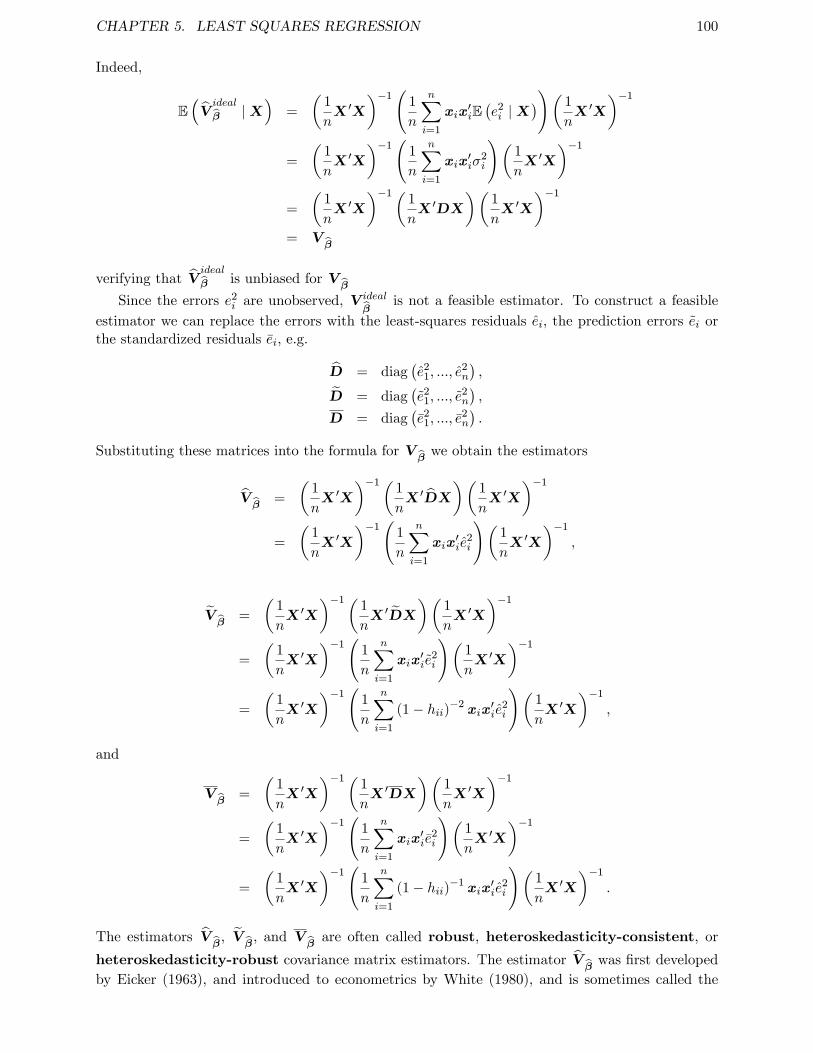
CHAPTER 5. LEAST SQUARES REGRESSION 100
Indeed,
E(Videal
β |X)
=
(1
nX ′X
)−1(
1
n
n∑i=1
xix′iE(e2i |X
))( 1
nX ′X
)−1
=
(1
nX ′X
)−1(
1
n
n∑i=1
xix′iσ
2i
)(1
nX ′X
)−1
=
(1
nX ′X
)−1( 1
nX ′DX
)(1
nX ′X
)−1
= Vβ
verifying that Videal
β is unbiased for Vβ
Since the errors e2i are unobserved, V
idealβ
is not a feasible estimator. To construct a feasibleestimator we can replace the errors with the least-squares residuals ei, the prediction errors ei orthe standardized residuals ei, e.g.
D = diag(e2
1, ..., e2n
),
D = diag(e2
1, ..., e2n
),
D = diag(e2
1, ..., e2n
).
Substituting these matrices into the formula for Vβwe obtain the estimators
Vβ
=
(1
nX ′X
)−1( 1
nX ′DX
)(1
nX ′X
)−1
=
(1
nX ′X
)−1(
1
n
n∑i=1
xix′ie
2i
)(1
nX ′X
)−1
,
Vβ
=
(1
nX ′X
)−1( 1
nX ′DX
)(1
nX ′X
)−1
=
(1
nX ′X
)−1(
1
n
n∑i=1
xix′ie
2i
)(1
nX ′X
)−1
=
(1
nX ′X
)−1(
1
n
n∑i=1
(1− hii)−2 xix′ie
2i
)(1
nX ′X
)−1
,
and
Vβ
=
(1
nX ′X
)−1( 1
nX ′DX
)(1
nX ′X
)−1
=
(1
nX ′X
)−1(
1
n
n∑i=1
xix′ie
2i
)(1
nX ′X
)−1
=
(1
nX ′X
)−1(
1
n
n∑i=1
(1− hii)−1 xix′ie
2i
)(1
nX ′X
)−1
.
The estimators Vβ, V
β, and V
βare often called robust, heteroskedasticity-consistent, or
heteroskedasticity-robust covariance matrix estimators. The estimator Vβwas first developed
by Eicker (1963), and introduced to econometrics by White (1980), and is sometimes called the
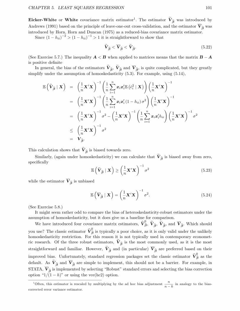
CHAPTER 5. LEAST SQUARES REGRESSION 101
Eicker-White or White covariance matrix estimator1. The estimator Vβwas introduced by
Andrews (1991) based on the principle of leave-one-out cross-validation, and the estimator Vβwas
introduced by Horn, Horn and Duncan (1975) as a reduced-bias covariance matrix estimator.Since (1− hii)−2 > (1− hii)−1 > 1 it is straightforward to show that
Vβ< V
β< V
β. (5.22)
(See Exercise 5.7.) The inequality A < B when applied to matrices means that the matrix B −Ais positive definite
In general, the bias of the estimators Vβ, V
βand V
β, is quite complicated, but they greatly
simplify under the assumption of homoskedasticity (5.3). For example, using (5.14),
E(Vβ|X)
=
(1
nX ′X
)−1(
1
n
n∑i=1
xix′iE(e2i |X
))( 1
nX ′X
)−1
=
(1
nX ′X
)−1(
1
n
n∑i=1
xix′i (1− hii)σ2
)(1
nX ′X
)−1
=
(1
nX ′X
)−1
σ2 −(
1
nX ′X
)−1(
1
n
n∑i=1
xix′ihii
)(1
nX ′X
)−1
σ2
≤(
1
nX ′X
)−1
σ2
= Vβ.
This calculation shows that Vβis biased towards zero.
Similarly, (again under homoskedasticity) we can calculate that Vβis biased away from zero,
specifically
E(Vβ|X)≥(
1
nX ′X
)−1
σ2 (5.23)
while the estimator Vβis unbiased
E(Vβ|X)
=
(1
nX ′X
)−1
σ2. (5.24)
(See Exercise 5.8.)It might seem rather odd to compare the bias of heteroskedasticity-robust estimators under the
assumption of homoskedasticity, but it does give us a baseline for comparison.
We have introduced four covariance matrix estimators, V0
β, V β, V
β, and V
β. Which should
you use? The classic estimator V0
β is typically a poor choice, as it is only valid under the unlikelyhomoskedasticity restriction. For this reason it is not typically used in contemporary economet-ric research. Of the three robust estimators, V
βis the most commonly used, as it is the most
straightforward and familiar. However, Vβand (in particular) V
βare preferred based on their
improved bias. Unfortunately, standard regression packages set the classic estimator V0
β as the
default. As Vβand V
βare simple to implement, this should not be a barrier. For example, in
STATA, Vβis implemented by selecting “Robust”standard errors and selecting the bias correction
option “1/(1− h)”or using the vce(hc2) option.
1Often, this estimator is rescaled by multiplying by the ad hoc bias adjustmentn
n− k in analogy to the bias-
corrected error variance estimator.
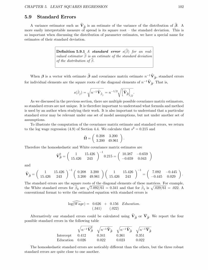
CHAPTER 5. LEAST SQUARES REGRESSION 102
5.9 Standard Errors
A variance estimator such as Vβis an estimate of the variance of the distribution of β. A
more easily interpretable measure of spread is its square root — the standard deviation. This isso important when discussing the distribution of parameter estimates, we have a special name forestimates of their standard deviation.
Definition 5.9.1 A standard error s(β) for an real-valued estimator β is an estimate of the standard deviationof the distribution of β.
When β is a vector with estimate β and covariance matrix estimate n−1Vβ, standard errors
for individual elements are the square roots of the diagonal elements of n−1Vβ. That is,
s(βj) =
√n−1V βj
= n−1/2
√[Vβ
]jj.
As we discussed in the previous section, there are multiple possible covariance matrix estimators,so standard errors are not unique. It is therefore important to understand what formula and methodis used by an author when studying their work. It is also important to understand that a particularstandard error may be relevant under one set of model assumptions, but not under another set ofassumptions.
To illustrate the computation of the covariance matrix estimate and standard errors, we returnto the log wage regression (4.9) of Section 4.4. We calculate that s2 = 0.215 and
Ω =
(0.208 3.2003.200 49.961
).
Therefore the homoskedastic and White covariance matrix estimates are
V0
β =
(1 15.426
15.426 243
)−1
0.215 =
(10.387 −0.659−0.659 0.043
)and
Vβ
=
(1 15.426
15.426 243
)−1(0.208 3.2003.200 49.961
)(1 15.426
15.426 243
)−1
=
(7.092 −0.445−0.445 0.029
).
The standard errors are the square roots of the diagonal elements of these matrices. For example,the White standard errors for β0 are
√7.092/61 = 0.341 and that for β1 is
√.029/61 = .022. A
conventional format to write the estimated equation with standard errors is
log(Wage) = 0.626(.341)
+ 0.156(.022)
Education.
Alternatively our standard errors could be calculated using Vβor V
β. We report the four
possible standard errors in the following table√n−1V
0
β
√n−1V
β
√n−1V
β
√n−1V
β
Intercept 0.412 0.341 0.361 0.351Education 0.026 0.022 0.023 0.022
The homoskedastic standard errors are noticably different than the others, but the three robuststandard errors are quite close to one another.
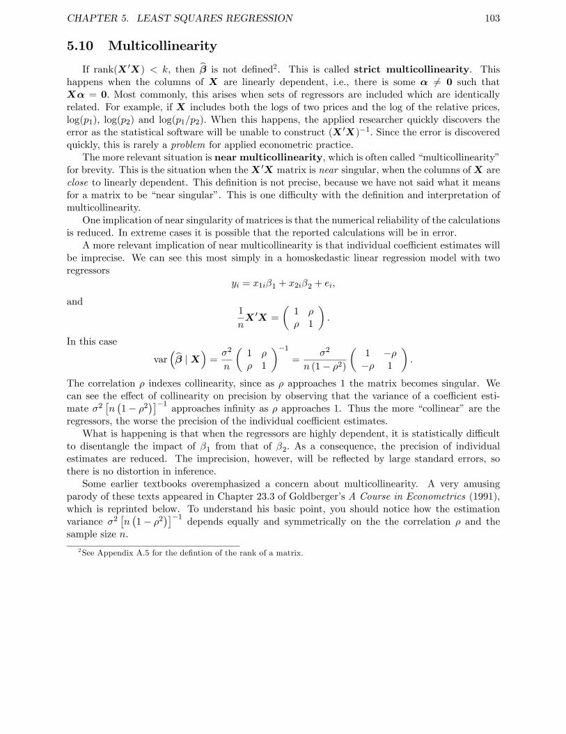
CHAPTER 5. LEAST SQUARES REGRESSION 103
5.10 Multicollinearity
If rank(X ′X) < k, then β is not defined2. This is called strict multicollinearity. Thishappens when the columns of X are linearly dependent, i.e., there is some α 6= 0 such thatXα = 0. Most commonly, this arises when sets of regressors are included which are identicallyrelated. For example, if X includes both the logs of two prices and the log of the relative prices,log(p1), log(p2) and log(p1/p2). When this happens, the applied researcher quickly discovers theerror as the statistical software will be unable to construct (X ′X)−1. Since the error is discoveredquickly, this is rarely a problem for applied econometric practice.
The more relevant situation is near multicollinearity, which is often called “multicollinearity”for brevity. This is the situation when theX ′X matrix is near singular, when the columns ofX areclose to linearly dependent. This definition is not precise, because we have not said what it meansfor a matrix to be “near singular”. This is one diffi culty with the definition and interpretation ofmulticollinearity.
One implication of near singularity of matrices is that the numerical reliability of the calculationsis reduced. In extreme cases it is possible that the reported calculations will be in error.
A more relevant implication of near multicollinearity is that individual coeffi cient estimates willbe imprecise. We can see this most simply in a homoskedastic linear regression model with tworegressors
yi = x1iβ1 + x2iβ2 + ei,
and1
nX ′X =
(1 ρρ 1
).
In this case
var(β |X
)=σ2
n
(1 ρρ 1
)−1
=σ2
n (1− ρ2)
(1 −ρ−ρ 1
).
The correlation ρ indexes collinearity, since as ρ approaches 1 the matrix becomes singular. Wecan see the effect of collinearity on precision by observing that the variance of a coeffi cient esti-mate σ2
[n(1− ρ2
)]−1 approaches infinity as ρ approaches 1. Thus the more “collinear” are theregressors, the worse the precision of the individual coeffi cient estimates.
What is happening is that when the regressors are highly dependent, it is statistically diffi cultto disentangle the impact of β1 from that of β2. As a consequence, the precision of individualestimates are reduced. The imprecision, however, will be reflected by large standard errors, sothere is no distortion in inference.
Some earlier textbooks overemphasized a concern about multicollinearity. A very amusingparody of these texts appeared in Chapter 23.3 of Goldberger’s A Course in Econometrics (1991),which is reprinted below. To understand his basic point, you should notice how the estimationvariance σ2
[n(1− ρ2
)]−1 depends equally and symmetrically on the the correlation ρ and thesample size n.
2See Appendix A.5 for the defintion of the rank of a matrix.

CHAPTER 5. LEAST SQUARES REGRESSION 104
Arthur S. Goldberger
Art Goldberger (1930-2009) was one of the most distinguished members of the Depart-ment of Economics at the University of Wisconsin. His PhD thesis developed an earlymacroeconometric forecasting model (known as the Klein-Goldberger model) but most ofhis career focused on microeconometric issues. He was the leading pioneer of what has beencalled the Wisconsin Tradition of empirical work — a combination of formal econometrictheory with a careful critical analysis of empirical work. Goldberger wrote a series of highlyregarded and influential graduate econometric textbooks, including including EconometricTheory (1964), Topics in Regression Analysis (1968), and A Course in Econometrics (1991).

CHAPTER 5. LEAST SQUARES REGRESSION 105
MicronumerosityArthur S. Goldberger
A Course in Econometrics (1991), Chapter 23.3
Econometrics texts devote many pages to the problem of multicollinearity in multiple regres-sion, but they say little about the closely analogous problem of small sample size in estimationa univariate mean. Perhaps that imbalance is attributable to the lack of an exotic polysyllabicname for “small sample size.” If so, we can remove that impediment by introducing the termmicronumerosity.
Suppose an econometrician set out to write a chapter about small sample size in samplingfrom a univariate population. Judging from what is now written about multicollinearity, thechapter might look like this:
1. Micronumerosity
The extreme case, “exact micronumerosity,” arises when n = 0, in which case the sampleestimate of µ is not unique. (Technically, there is a violation of the rank condition n > 0 : thematrix 0 is singular.) The extreme case is easy enough to recognize. “Near micronumerosity”is more subtle, and yet very serious. It arises when the rank condition n > 0 is barelysatisfied. Near micronumerosity is very prevalent in empirical economics.
2. Consequences of micronumerosity
The consequences of micronumerosity are serious. Precision of estimation is reduced. Thereare two aspects of this reduction: estimates of µ may have large errors, and not only that,but Vy will be large.
Investigators will sometimes be led to accept the hypothesis µ = 0 because y/σy is small,even though the true situation may be not that µ = 0 but simply that the sample data havenot enabled us to pick µ up.
The estimate of µ will be very sensitive to sample data, and the addition of a few moreobservations can sometimes produce drastic shifts in the sample mean.
The true µ may be suffi ciently large for the null hypothesis µ = 0 to be rejected, eventhough Vy = σ2/n is large because of micronumerosity. But if the true µ is small (althoughnonzero) the hypothesis µ = 0 may mistakenly be accepted.
3. Testing for micronumerosity
Tests for the presence of micronumerosity require the judicious use of various fingers. Someresearchers prefer a single finger, others use their toes, still others let their thumbs rule.
A generally reliable guide may be obtained by counting the number of observations. Mostof the time in econometric analysis, when n is close to zero, it is also far from infinity.
Several test procedures develop critical values n∗, such that micronumerosity is a problemonly if n is smaller than n∗. But those procedures are questionable.
4. Remedies for micronumerosity
If micronumerosity proves serious in the sense that the estimate of µ has an unsatisfactorilylow degree of precision, we are in the statistical position of not being able to make brickswithout straw. The remedy lies essentially in the acquisition, if possible, of larger samplesfrom the same population.
But more data are no remedy for micronumerosity if the additional data are simply “moreof the same.”So obtaining lots of small samples from the same population will not help.
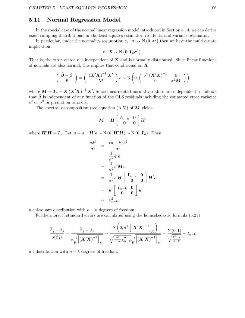
CHAPTER 5. LEAST SQUARES REGRESSION 106
5.11 Normal Regression Model
In the special case of the normal linear regression model introduced in Section 4.14, we can deriveexact sampling distributions for the least-squares estimator, residuals, and variance estimator.
In particular, under the normality assumption ei | xi ∼ N(0, σ2
)then we have the multivariate
implicatione |X ∼ N
(0, Inσ
2).
That is, the error vector e is independent of X and is normally distributed. Since linear functionsof normals are also normal, this implies that conditional on X(
β − βe
)=
((X ′X)
−1X ′
M
)e ∼ N
(0,
(σ2 (X ′X)
−10
0 σ2M
))where M = In −X (X ′X)
−1X ′. Since uncorrelated normal variables are independent, it follows
that β is independent of any function of the OLS residuals including the estimated error variances2 or σ2 or prediction errors e.
The spectral decomposition (see equation (A.5)) ofM yields
M = H
[In−k 0
0 0
]H ′
where H ′H = In. Let u = σ−1H ′e ∼ N (0,H ′H) ∼ N (0, In) . Then
nσ2
σ2=
(n− k) s2
σ2
=1
σ2e′e
=1
σ2e′Me
=1
σ2e′H
[In−k 0
0 0
]H ′e
= u′[In−k 0
0 0
]u
∼ χ2n−k,
a chi-square distribution with n− k degrees of freedom.Furthermore, if standard errors are calculated using the homoskedastic formula (5.21)
βj − βjs(βj)
=βj − βj
s
√[(X ′X)
−1]jj
∼N
(0, σ2
[(X ′X)
−1]jj
)√
σ2
n−kχ2n−k
√[(X ′X)
−1]jj
=N (0, 1)√
χ2n−kn−k
∼ tn−k
a t distribution with n− k degrees of freedom.
CHAPTER 5. LEAST SQUARES REGRESSION 107
Theorem 5.11.1 Normal RegressionIn the linear regression model (Assumption 5.1.1) if ei is independent ofxi and distributed N
(0, σ2
)then
• β − β ∼ N(0, σ2 (X ′X)
−1)
• nσ2
σ2= (n−k)s2
σ2∼ χ2
n−k
• βj−βjs(βj)
∼ tn−k
These are the exact finite-sample distributions of the least-squares estimator and variance esti-mators, and are the basis for traditional inference in linear regression.
While elegant, the diffi culty in applying Theorem 5.11.1 is that the normality assumption istoo restrictive to be empirical plausible, and therefore inference based on Theorem 5.11.1 has noguarantee of accuracy. We develop a more broadly-applicable inference theory based on largesample (asymptotic) approximations in the following chapter.
William Gosset
William S. Gosset (1876-1937) of England is most famous for his derivation of the student’st distribution, published in the paper “The probable error of a mean”in 1908. At the time,Gosset worked at Guiness Brewery, which prohibited its employees from publishing in orderto prevent the possible loss of trade secrets. To circumvent this barrier, Gosset publishedunder the pseudonym “Student”. Consequently, this famous distribution is known as thestudent’s t rather than Gosset’s t!
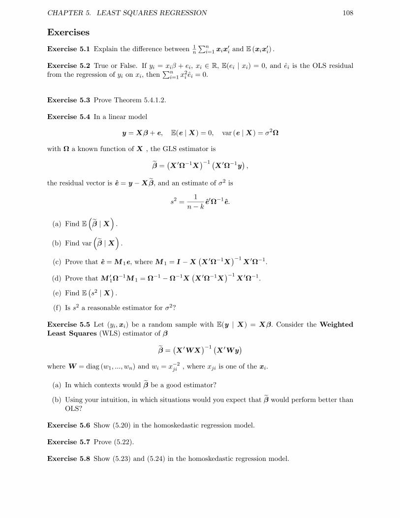
CHAPTER 5. LEAST SQUARES REGRESSION 108
Exercises
Exercise 5.1 Explain the difference between 1n
∑ni=1 xix
′i and E (xix
′i) .
Exercise 5.2 True or False. If yi = xiβ + ei, xi ∈ R, E(ei | xi) = 0, and ei is the OLS residualfrom the regression of yi on xi, then
∑ni=1 x
2i ei = 0.
Exercise 5.3 Prove Theorem 5.4.1.2.
Exercise 5.4 In a linear model
y = Xβ + e, E(e |X) = 0, var (e |X) = σ2Ω
with Ω a known function of X , the GLS estimator is
β =(X ′Ω−1X
)−1 (X ′Ω−1y
),
the residual vector is e = y −Xβ, and an estimate of σ2 is
s2 =1
n− k e′Ω−1e.
(a) Find E(β |X
).
(b) Find var(β |X
).
(c) Prove that e = M1e, whereM1 = I −X(X ′Ω−1X
)−1X ′Ω−1.
(d) Prove thatM ′1Ω−1M1 = Ω−1 −Ω−1X
(X ′Ω−1X
)−1X ′Ω−1.
(e) Find E(s2 |X
).
(f) Is s2 a reasonable estimator for σ2?
Exercise 5.5 Let (yi,xi) be a random sample with E(y | X) = Xβ. Consider the WeightedLeast Squares (WLS) estimator of β
β =(X ′WX
)−1 (X ′Wy
)where W = diag (w1, ..., wn) and wi = x−2
ji , where xji is one of the xi.
(a) In which contexts would β be a good estimator?
(b) Using your intuition, in which situations would you expect that β would perform better thanOLS?
Exercise 5.6 Show (5.20) in the homoskedastic regression model.
Exercise 5.7 Prove (5.22).
Exercise 5.8 Show (5.23) and (5.24) in the homoskedastic regression model.
Chapter 6
Asymptotic Theory for Least Squares
6.1 Introduction
In the previous chapter we derived the mean and variance of the least-squares estimator in thecontext of the linear regression model, but this is not a complete description of the sampling dis-tribution, nor suffi cient for inference (confidence intervals and hypothesis testing) on the unknownparameters. Furthermore, the theory does not apply in the context of the linear projection model,which is more relevant for empirical applications.
To illustrate the situation with an example, let yi and xi be drawn from the joint density
f(x, y) =1
2πxyexp
(−1
2(log y − log x)2
)exp
(−1
2(log x)2
)and let β be the slope coeffi cient estimate from a least-squares regression of yi on xi and a constant.Using simulation methods, the density function of β was computed and plotted in Figure 6.1 forsample sizes of n = 25, n = 100 and n = 800. The vertical line marks the true projection coeffi cient.
From the figure we can see that the density functions are dispersed and highly non-normal. Asthe sample size increases the density becomes more concentrated about the population coeffi cient.Is there a simple way to characterize the sampling distribution of β?
In principle the sampling distribution of β is a function of the joint distribution of (yi, xi)and the sample size n, but in practice this function is extremely complicated so it is not feasible toanalytically calculate the exact distribution of β except in very special cases. Therefore we typicallyrely on approximation methods.
The most widely used and versatile method is asymptotic theory, which approximates samplingdistributions by taking the limit of the finite sample distribution as the sample size n tends toinfinity. The primary tools of asymptotic theory are the weak law of large numbers (WLLN),central limit theorem (CLT), and continuous mapping theorem (CMT), which were reviewed inChapter 2. With these tools we can approximate the sampling distributions of most econometricestimators.
It turns out that the asymptotic theory of least-squares estimation applies equally to the pro-jection model and the linear CEF model, and therefore the results in this chapter will be stated forthe broader projection model (Assumption 1.5.1 and Assumption 3.16.1).
6.2 Consistency of Least-Squares Estimation
In this section we use the weak law of large numbers (WLLN, Theorem 2.6.1 and Theorem 2.7.2)and continuous mapping theorem (CMT, Theorem 2.9.1) to show that the least-squares estimatorβ is consistent for the projection coeffi cient β.
This derivation is based on three key components. First, the OLS estimator can be written asa continuous function of a set of sample moments. Second, the WLLN shows that sample moments
109
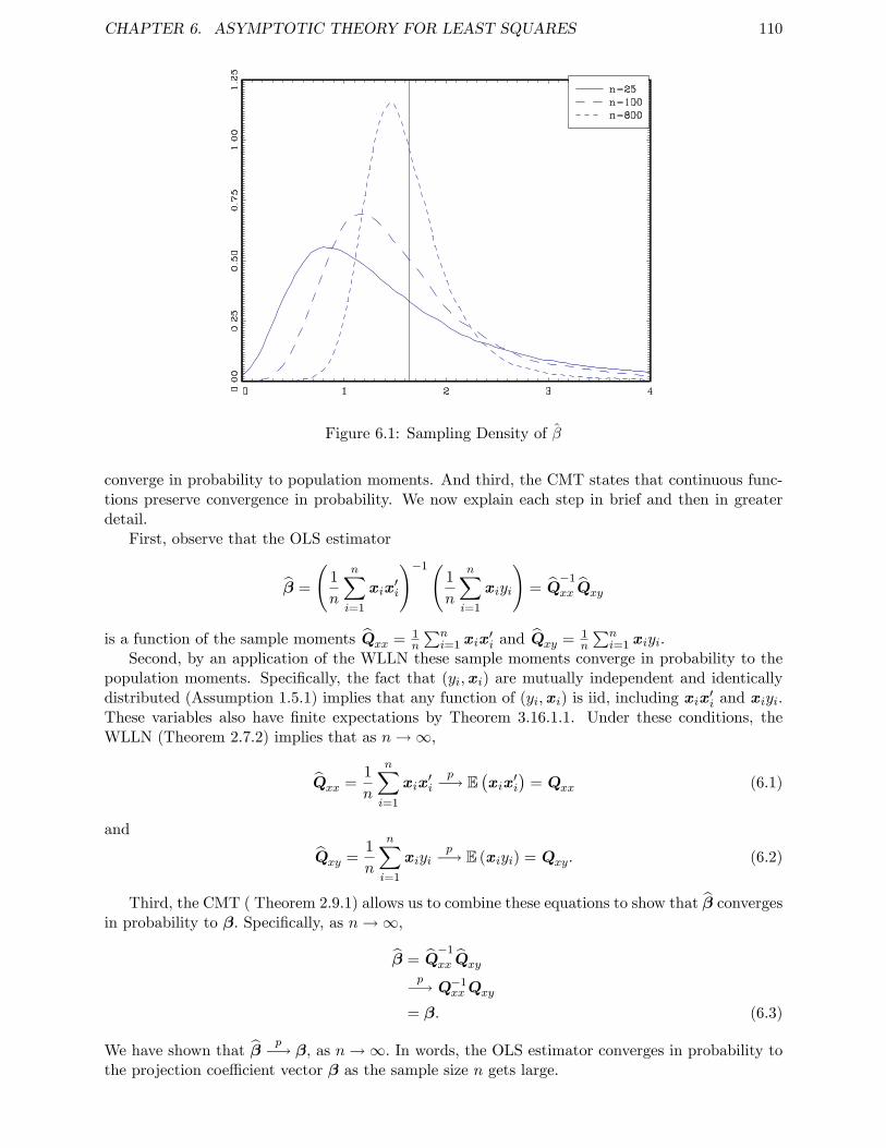
CHAPTER 6. ASYMPTOTIC THEORY FOR LEAST SQUARES 110
Figure 6.1: Sampling Density of β
converge in probability to population moments. And third, the CMT states that continuous func-tions preserve convergence in probability. We now explain each step in brief and then in greaterdetail.
First, observe that the OLS estimator
β =
(1
n
n∑i=1
xix′i
)−1(1
n
n∑i=1
xiyi
)= Q
−1
xx Qxy
is a function of the sample moments Qxx = 1n
∑ni=1 xix
′i and Qxy = 1
n
∑ni=1 xiyi.
Second, by an application of the WLLN these sample moments converge in probability to thepopulation moments. Specifically, the fact that (yi,xi) are mutually independent and identicallydistributed (Assumption 1.5.1) implies that any function of (yi,xi) is iid, including xix′i and xiyi.These variables also have finite expectations by Theorem 3.16.1.1. Under these conditions, theWLLN (Theorem 2.7.2) implies that as n→∞,
Qxx =1
n
n∑i=1
xix′i
p−→ E(xix
′i
)= Qxx (6.1)
and
Qxy =1
n
n∑i=1
xiyip−→ E (xiyi) = Qxy. (6.2)
Third, the CMT ( Theorem 2.9.1) allows us to combine these equations to show that β convergesin probability to β. Specifically, as n→∞,
β = Q−1
xx Qxy
p−→ Q−1xxQxy
= β. (6.3)
We have shown that βp−→ β, as n→∞. In words, the OLS estimator converges in probability to
the projection coeffi cient vector β as the sample size n gets large.
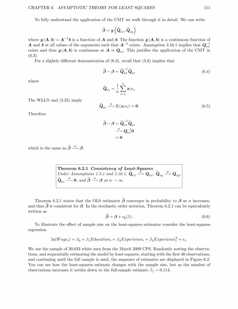
CHAPTER 6. ASYMPTOTIC THEORY FOR LEAST SQUARES 111
To fully understand the application of the CMT we walk through it in detail. We can write
β = g(Qxx, Qxy
)where g (A, b) = A−1b is a function of A and b. The function g (A, b) is a continuous function ofA and b at all values of the arguments such that A−1 exists. Assumption 3.16.1 implies that Q−1
xx
exists and thus g (A, b) is continuous at A = Qxx. This justifies the application of the CMT in(6.3).
For a slightly different demonstration of (6.3), recall that (5.6) implies that
β − β = Q−1
xx Qxe (6.4)
where
Qxe =1
n
n∑i=1
xiei.
The WLLN and (3.25) implyQxe
p−→ E (xiei) = 0. (6.5)
Therefore
β − β = Q−1
xx Qxep−→ Q−1
xx0
= 0
which is the same as βp−→ β.
Theorem 6.2.1 Consistency of Least-SquaresUnder Assumptions 1.5.1 and 3.16.1, Qxx
p−→ Qxx, Qxyp−→ Qxy,
Qxep−→ 0, and β
p−→ β as n→∞.
Theorem 6.2.1 states that the OLS estimator β converges in probability to β as n increases,and thus β is consistent for β. In the stochastic order notation, Theorem 6.2.1 can be equivalentlywritten as
β = β + op(1). (6.6)
To illustrate the effect of sample size on the least-squares estimator consider the least-squaresregression
ln(Wagei) = β0 + β1Educationi + β2Experiencei + β3Experience2i + ei.
We use the sample of 30,833 white men from the March 2009 CPS. Randomly sorting the observa-tions, and sequentially estimating the model by least-squares, starting with the first 40 observations,and continuing until the full sample is used, the sequence of estimates are displayed in Figure 6.2.You can see how the least-squares estimate changes with the sample size, but as the number ofobservations increases it settles down to the full-sample estimate β1 = 0.114.
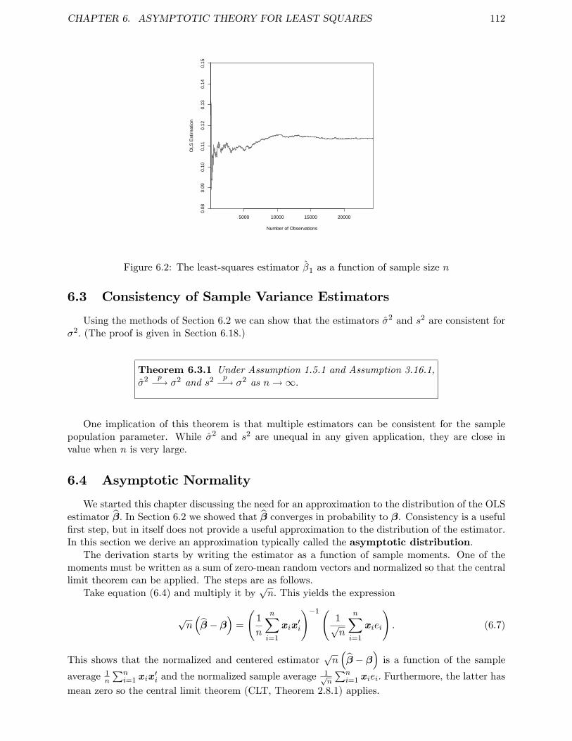
CHAPTER 6. ASYMPTOTIC THEORY FOR LEAST SQUARES 112
5000 10000 15000 20000
0.08
0.09
0.10
0.11
0.12
0.13
0.14
0.15
Number of Observations
OLS
Est
imat
ion
Figure 6.2: The least-squares estimator β1 as a function of sample size n
6.3 Consistency of Sample Variance Estimators
Using the methods of Section 6.2 we can show that the estimators σ2 and s2 are consistent forσ2. (The proof is given in Section 6.18.)
Theorem 6.3.1 Under Assumption 1.5.1 and Assumption 3.16.1,σ2 p−→ σ2 and s2 p−→ σ2 as n→∞.
One implication of this theorem is that multiple estimators can be consistent for the samplepopulation parameter. While σ2 and s2 are unequal in any given application, they are close invalue when n is very large.
6.4 Asymptotic Normality
We started this chapter discussing the need for an approximation to the distribution of the OLSestimator β. In Section 6.2 we showed that β converges in probability to β. Consistency is a usefulfirst step, but in itself does not provide a useful approximation to the distribution of the estimator.In this section we derive an approximation typically called the asymptotic distribution.
The derivation starts by writing the estimator as a function of sample moments. One of themoments must be written as a sum of zero-mean random vectors and normalized so that the centrallimit theorem can be applied. The steps are as follows.
Take equation (6.4) and multiply it by√n. This yields the expression
√n(β − β
)=
(1
n
n∑i=1
xix′i
)−1(1√n
n∑i=1
xiei
). (6.7)
This shows that the normalized and centered estimator√n(β − β
)is a function of the sample
average 1n
∑ni=1 xix
′i and the normalized sample average
1√n
∑ni=1 xiei. Furthermore, the latter has
mean zero so the central limit theorem (CLT, Theorem 2.8.1) applies.
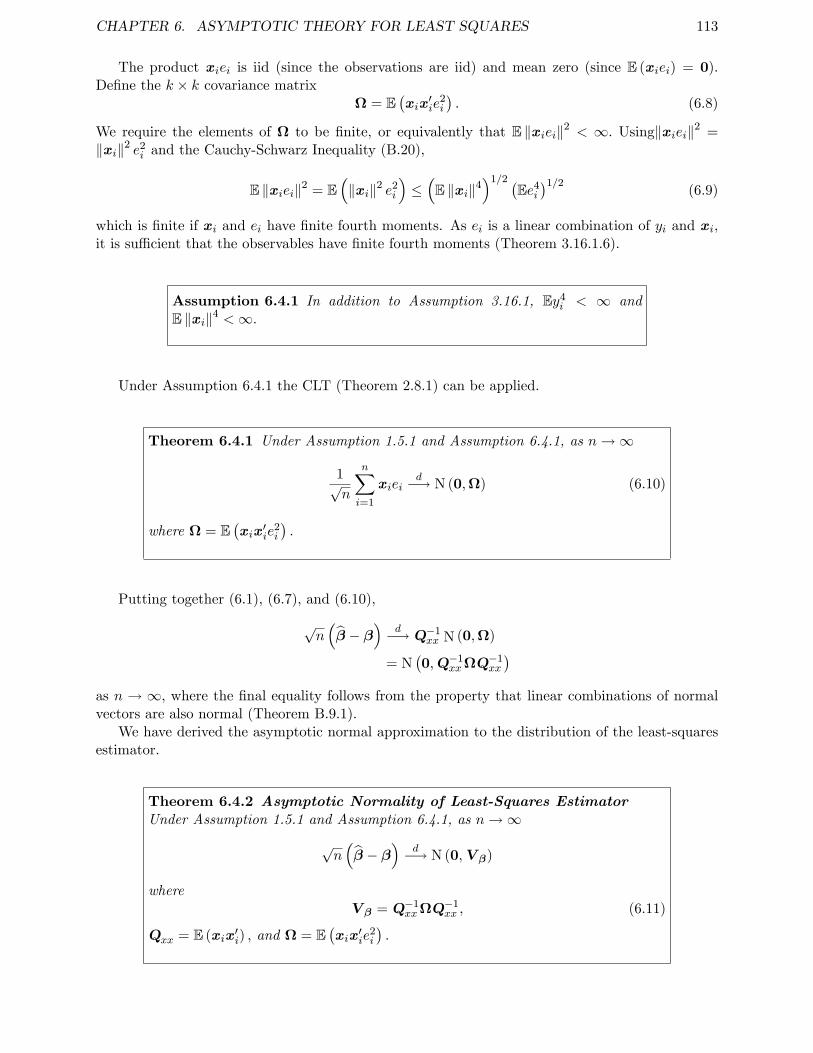
CHAPTER 6. ASYMPTOTIC THEORY FOR LEAST SQUARES 113
The product xiei is iid (since the observations are iid) and mean zero (since E (xiei) = 0).Define the k × k covariance matrix
Ω = E(xix
′ie
2i
). (6.8)
We require the elements of Ω to be finite, or equivalently that E ‖xiei‖2 < ∞. Using‖xiei‖2 =‖xi‖2 e2
i and the Cauchy-Schwarz Inequality (B.20),
E ‖xiei‖2 = E(‖xi‖2 e2
i
)≤(E ‖xi‖4
)1/2 (Ee4
i
)1/2(6.9)
which is finite if xi and ei have finite fourth moments. As ei is a linear combination of yi and xi,it is suffi cient that the observables have finite fourth moments (Theorem 3.16.1.6).
Assumption 6.4.1 In addition to Assumption 3.16.1, Ey4i < ∞ and
E ‖xi‖4 <∞.
Under Assumption 6.4.1 the CLT (Theorem 2.8.1) can be applied.
Theorem 6.4.1 Under Assumption 1.5.1 and Assumption 6.4.1, as n→∞
1√n
n∑i=1
xieid−→ N (0,Ω) (6.10)
where Ω = E(xix
′ie
2i
).
Putting together (6.1), (6.7), and (6.10),
√n(β − β
)d−→ Q−1
xx N (0,Ω)
= N(0,Q−1
xxΩQ−1xx
)as n → ∞, where the final equality follows from the property that linear combinations of normalvectors are also normal (Theorem B.9.1).
We have derived the asymptotic normal approximation to the distribution of the least-squaresestimator.
Theorem 6.4.2 Asymptotic Normality of Least-Squares EstimatorUnder Assumption 1.5.1 and Assumption 6.4.1, as n→∞
√n(β − β
)d−→ N (0,V β)
whereV β = Q−1
xxΩQ−1xx , (6.11)
Qxx = E (xix′i) , and Ω = E
(xix
′ie
2i
).
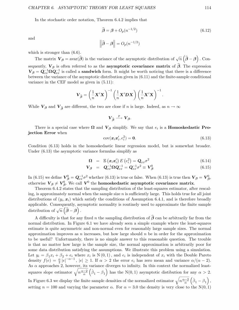
CHAPTER 6. ASYMPTOTIC THEORY FOR LEAST SQUARES 114
In the stochastic order notation, Theorem 6.4.2 implies that
β = β +Op(n−1/2) (6.12)
and ∥∥∥β − β∥∥∥ = Op(n−1/2)
which is stronger than (6.6).
The matrix V β = avar(β) is the variance of the asymptotic distribution of√n(β − β
). Con-
sequently, V β is often referred to as the asymptotic covariance matrix of β. The expressionV β = Q−1
xxΩQ−1xx is called a sandwich form. It might be worth noticing that there is a difference
between the variance of the asymptotic distribution given in (6.11) and the finite-sample conditionalvariance in the CEF model as given in (5.11):
Vβ
=
(1
nX ′X
)−1( 1
nX ′DX
)(1
nX ′X
)−1
.
While V β and V βare different, the two are close if n is large. Indeed, as n→∞
Vβ
p−→ V β.
There is a special case where Ω and V β simplify. We say that ei is a Homoskedastic Pro-jection Error when
cov(xix′i, e
2i ) = 0. (6.13)
Condition (6.13) holds in the homoskedastic linear regression model, but is somewhat broader.Under (6.13) the asymptotic variance formulas simplify as
Ω = E(xix
′i
)E(e2i
)= Qxxσ
2 (6.14)
V β = Q−1xxΩQ−1
xx = Q−1xxσ
2 ≡ V 0β (6.15)
In (6.15) we define V 0β = Q−1
xxσ2 whether (6.13) is true or false. When (6.13) is true then V β = V 0
β,
otherwise V β 6= V 0β. We call V
0 the homoskedastic asymptotic covariance matrix.Theorem 6.4.2 states that the sampling distribution of the least-squares estimator, after rescal-
ing, is approximately normal when the sample size n is suffi ciently large. This holds true for all jointdistributions of (yi,xi) which satisfy the conditions of Assumption 6.4.1, and is therefore broadlyapplicable. Consequently, asymptotic normality is routinely used to approximate the finite sample
distribution of√n(β − β
).
A diffi culty is that for any fixed n the sampling distribution of β can be arbitrarily far from thenormal distribution. In Figure 6.1 we have already seen a simple example where the least-squaresestimate is quite asymmetric and non-normal even for reasonably large sample sizes. The normalapproximation improves as n increases, but how large should n be in order for the approximationto be useful? Unfortunately, there is no simple answer to this reasonable question. The troubleis that no matter how large is the sample size, the normal approximation is arbitrarily poor forsome data distribution satisfying the assumptions. We illustrate this problem using a simulation.Let yi = β1xi + β2 + ei where xi is N (0, 1) , and ei is independent of xi with the Double Paretodensity f(e) = α
2 |e|−α−1 , |e| ≥ 1. If α > 2 the error ei has zero mean and variance α/(α − 2).
As α approaches 2, however, its variance diverges to infinity. In this context the normalized least-
squares slope estimator√nα−2
α
(β1 − β1
)has the N(0, 1) asymptotic distibution for any α > 2.
In Figure 6.3 we display the finite sample densities of the normalized estimator√nα−2
α
(β1 − β1
),
setting n = 100 and varying the parameter α. For α = 3.0 the density is very close to the N(0, 1)
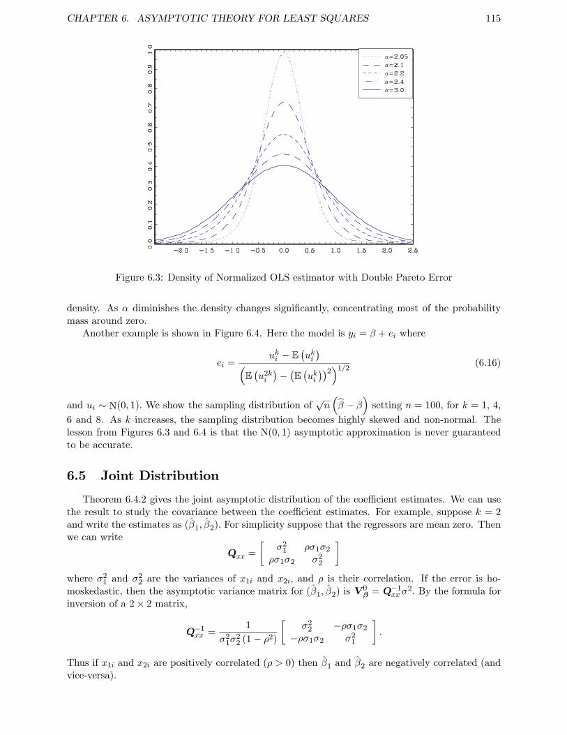
CHAPTER 6. ASYMPTOTIC THEORY FOR LEAST SQUARES 115
Figure 6.3: Density of Normalized OLS estimator with Double Pareto Error
density. As α diminishes the density changes significantly, concentrating most of the probabilitymass around zero.
Another example is shown in Figure 6.4. Here the model is yi = β + ei where
ei =uki − E
(uki)(
E(u2ki
)−(E(uki))2)1/2
(6.16)
and ui ∼ N(0, 1). We show the sampling distribution of√n(β − β
)setting n = 100, for k = 1, 4,
6 and 8. As k increases, the sampling distribution becomes highly skewed and non-normal. Thelesson from Figures 6.3 and 6.4 is that the N(0, 1) asymptotic approximation is never guaranteedto be accurate.
6.5 Joint Distribution
Theorem 6.4.2 gives the joint asymptotic distribution of the coeffi cient estimates. We can usethe result to study the covariance between the coeffi cient estimates. For example, suppose k = 2and write the estimates as (β1, β2). For simplicity suppose that the regressors are mean zero. Thenwe can write
Qxx =
[σ2
1 ρσ1σ2
ρσ1σ2 σ22
]where σ2
1 and σ22 are the variances of x1i and x2i, and ρ is their correlation. If the error is ho-
moskedastic, then the asymptotic variance matrix for (β1, β2) is V 0β = Q−1
xxσ2. By the formula for
inversion of a 2× 2 matrix,
Q−1xx =
1
σ21σ
22 (1− ρ2)
[σ2
2 −ρσ1σ2
−ρσ1σ2 σ21
].
Thus if x1i and x2i are positively correlated (ρ > 0) then β1 and β2 are negatively correlated (andvice-versa).
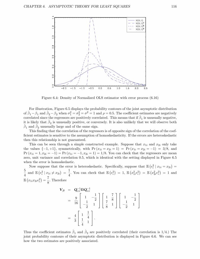
CHAPTER 6. ASYMPTOTIC THEORY FOR LEAST SQUARES 116
Figure 6.4: Density of Normalized OLS estimator with error process (6.16)
For illustration, Figure 6.5 displays the probability contours of the joint asymptotic distributionof β1−β1 and β2−β2 when σ
21 = σ2
2 = σ2 = 1 and ρ = 0.5. The coeffi cient estimates are negativelycorrelated since the regressors are positively correlated. This means that if β1 is unusually negative,it is likely that β2 is unusually positive, or conversely. It is also unlikely that we will observe bothβ1 and β2 unusually large and of the same sign.
This finding that the correlation of the regressors is of opposite sign of the correlation of the coef-ficient estimates is sensitive to the assumption of homoskedasticity. If the errors are heteroskedasticthen this relationship is not guaranteed.
This can be seen through a simple constructed example. Suppose that x1i and x2i only takethe values −1,+1, symmetrically, with Pr (x1i = x2i = 1) = Pr (x1i = x2i = −1) = 3/8, andPr (x1i = 1, x2i = −1) = Pr (x1i = −1, x2i = 1) = 1/8. You can check that the regressors are meanzero, unit variance and correlation 0.5, which is identical with the setting displayed in Figure 6.5when the error is homoskedastic.
Now suppose that the error is heteroskedastic. Specifically, suppose that E(e2i | x1i = x2i
)=
5
4and E
(e2i | x1i 6= x2i
)=
1
4. You can check that E
(e2i
)= 1, E
(x2
1ie2i
)= E
(x2
2ie2i
)= 1 and
E(x1ix2ie
2i
)=
7
8. Therefore
V β = Q−1xxΩQ−1
xx
=9
16
1 −1
2
−1
21
1
7
87
81
1 −1
2
−1
21
=4
3
11
41
41
.Thus the coeffi cient estimates β1 and β2 are positively correlated (their correlation is 1/4.) Thejoint probability contours of their asymptotic distribution is displayed in Figure 6.6. We can seehow the two estimates are positively associated.
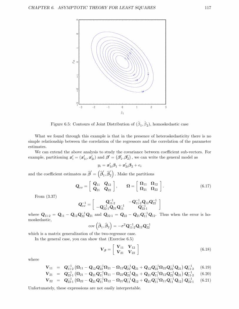
CHAPTER 6. ASYMPTOTIC THEORY FOR LEAST SQUARES 117
Figure 6.5: Contours of Joint Distribution of (β1, β2), homoskedastic case
What we found through this example is that in the presence of heteroskedasticity there is nosimple relationship between the correlation of the regressors and the correlation of the parameterestimates.
We can extend the above analysis to study the covariance between coeffi cient sub-vectors. Forexample, partitioning x′i = (x′1i,x
′2i) and β
′ =(β′1,β
′2
), we can write the general model as
yi = x′1iβ1 + x′2iβ2 + ei
and the coeffi cient estimates as β′=(β′1, β
′2
). Make the partitions
Qxx =
[Q11 Q12
Q21 Q22
], Ω =
[Ω11 Ω12
Ω21 Ω22
]. (6.17)
From (3.37)
Q−1xx =
[Q−1
11·2 −Q−111·2Q12Q
−122
−Q−122·1Q21Q
−111 Q−1
22·1
]where Q11·2 = Q11 − Q12Q
−122 Q21 and Q22·1 = Q22 − Q21Q
−111 Q12. Thus when the error is ho-
moskedastic,
cov(β1, β2
)= −σ2Q−1
11·2Q12Q−122
which is a matrix generalization of the two-regressor case.In the general case, you can show that (Exercise 6.5)
V β =
[V 11 V 12
V 21 V 22
](6.18)
where
V 11 = Q−111·2
(Ω11 −Q12Q
−122 Ω21 −Ω12Q
−122 Q21 +Q12Q
−122 Ω22Q
−122 Q21
)Q−1
11·2 (6.19)
V 21 = Q−122·1
(Ω21 −Q21Q
−111 Ω11 −Ω22Q
−122 Q21 +Q21Q
−111 Ω12Q
−122 Q21
)Q−1
11·2 (6.20)
V 22 = Q−122·1
(Ω22 −Q21Q
−111 Ω12 −Ω21Q
−111 Q12 +Q21Q
−111 Ω11Q
−111 Q12
)Q−1
22·1 (6.21)
Unfortunately, these expressions are not easily interpretable.
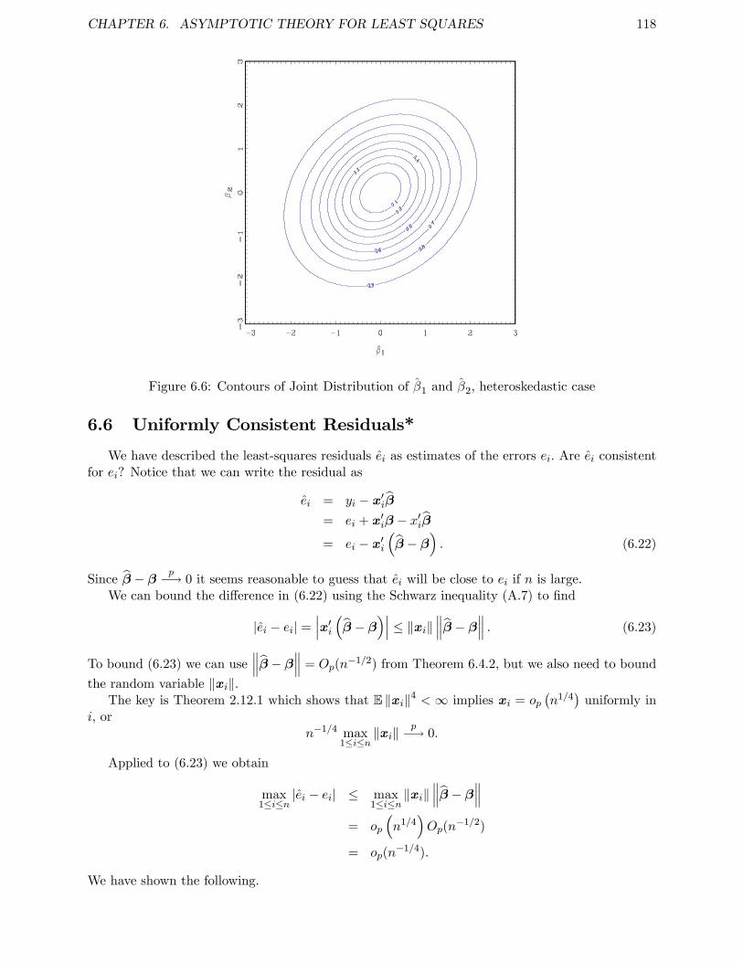
CHAPTER 6. ASYMPTOTIC THEORY FOR LEAST SQUARES 118
Figure 6.6: Contours of Joint Distribution of β1 and β2, heteroskedastic case
6.6 Uniformly Consistent Residuals*
We have described the least-squares residuals ei as estimates of the errors ei. Are ei consistentfor ei? Notice that we can write the residual as
ei = yi − x′iβ= ei + x′iβ − x′iβ= ei − x′i
(β − β
). (6.22)
Since β − β p−→ 0 it seems reasonable to guess that ei will be close to ei if n is large.We can bound the difference in (6.22) using the Schwarz inequality (A.7) to find
|ei − ei| =∣∣∣x′i (β − β)∣∣∣ ≤ ‖xi‖ ∥∥∥β − β∥∥∥ . (6.23)
To bound (6.23) we can use∥∥∥β − β∥∥∥ = Op(n
−1/2) from Theorem 6.4.2, but we also need to bound
the random variable ‖xi‖.The key is Theorem 2.12.1 which shows that E ‖xi‖4 < ∞ implies xi = op
(n1/4
)uniformly in
i, orn−1/4 max
1≤i≤n‖xi‖
p−→ 0.
Applied to (6.23) we obtain
max1≤i≤n
|ei − ei| ≤ max1≤i≤n
‖xi‖∥∥∥β − β∥∥∥
= op
(n1/4
)Op(n
−1/2)
= op(n−1/4).
We have shown the following.
CHAPTER 6. ASYMPTOTIC THEORY FOR LEAST SQUARES 119
Theorem 6.6.1 Under Assumptions 1.5.1 and 6.4.1, uniformly in 1 ≤ i ≤ n
ei = ei + op(n−1/4). (6.24)
What about the squared residuals e2i ? Squaring the two sides of (6.24) we obtain
e2i =
(ei + op(n
−1/4))2
= e2i + 2eiop(n
−1/4) + op(n−1/2)
= e2i + op(1) (6.25)
uniformly in 1 ≤ i ≤ n, since ei = op(n1/4
)when E |ei|4 <∞ by Theorem 2.12.1.
Theorem 6.6.2 Under Assumptions 1.5.1 and 6.4.1, uniformly in 1 ≤ i ≤ n
e2i = e2
i + op(1)
6.7 Asymptotic Leverage*
Recall the definition of leverage from (4.21)
hii = x′i(X ′X
)−1xi.
These are the diagonal elements of the projection matrix P and appear in the formula for leave-one-out prediction errors and several covariance matrix estimators. We can show that under iidsampling the leverage values are uniformly asymptotically small.
Let λmin(A) and λmax(A) denote the smallest and largest eigenvalues of a symmetric squarematrix A, and note that λmax(A−1) = (λmin(A))−1 .
Since 1nX
′Xp−→ Qxx > 0 then by the CMT, λmin
(1nX
′X) p−→ λmin (Qxx) > 0. (The latter is
positive since Qxx is positive definite and thus all its eigenvalues are positive.) Then by the TraceInequality (A.10)
hii = x′i(X ′X
)−1xi
= tr
((1
nX ′X
)−1 1
nxix
′i
)
≤ λmax
((1
nX ′X
)−1)
tr
(1
nxix
′i
)=
(λmin
(1
nX ′X
))−1 1
n‖xi‖2
≤ (λmin (Qxx) + op(1))−1 1
nmax
1≤i≤n‖xi‖2 . (6.26)
Theorem 2.12.1 shows that E ‖xi‖2 <∞ implies
n−1/2 max1≤i≤n
‖xi‖p−→ 0

CHAPTER 6. ASYMPTOTIC THEORY FOR LEAST SQUARES 120
and thusn−1 max
1≤i≤n‖xi‖2
p−→ 0.
It follows that (6.26) is op(1), uniformly in i.
Theorem 6.7.1 Under Assumption 1.5.1 and E ‖xi‖2 <∞, uniformly in1 ≤ i ≤ n, hii = op(1).
Theorem (6.7.1) implies that under random sampling with finite variances and large samples,no individual observation should have a large leverage value. Consequently individual observationsshould not be influential, unless one of these conditions is violated.
6.8 Consistent Covariance Matrix Estimation
In Sections 5.7 and 5.8 we introduced estimators of the finite-sample covariance matrix of theleast-squares estimator in the regression model. In this section we show that these estimators areconsistent for the asymptotic covariance matrix.
First, consider the covariance matrix estimate constructed under the assumption of homoskedas-ticity:
V0
β =
(1
nX ′X
)−1
s2 = Q−1
xx s2.
Since Qxxp−→ Qxx (Theorem 6.2.1), s
2 p−→ σ2 (Theorem 6.3.1), and Qxx is invertible (Assumption3.16.1), it follows that
V0
β = Q−1
xx s2 p−→ Q−1
xxσ2 = V 0
β
so that V0
β is consistent for V0β, the homoskedastic covariance matrix.
Theorem 6.8.1 Under Assumption 1.5.1 and Assumption 3.16.1,V
0
βp−→ V 0
β as n→∞.
Now consider the heteroskedasticity-robust covariance matrix estimators Vβ, V
β, and V
β.
Writing
Ω =1
n
n∑i=1
xix′ie
2i , (6.27)
Ω =1
n
n∑i=1
(1− hii)−2 xix′ie
2i
and
Ω =1
n
n∑i=1
(1− hii)−1 xix′ie
2i
as moment estimators for Ω = E(xix
′ie
2i
), then the covariance matrix estimators are
CHAPTER 6. ASYMPTOTIC THEORY FOR LEAST SQUARES 121
Vβ
= Q−1
xx ΩQ−1
xx ,
Vβ
= Q−1
xx ΩQ−1
xx ,
andVβ
= Q−1
xxΩQ−1
xx .
We can show that Ω, Ω, and Ω are consistent for Ω. Combined with the consistency of Qxx
for Qxx and the invertibility of Qxx we find that V β, V
β, and V
βconverge in probability to
Q−1xxΩQ−1
xx = V β. The complete proof is given in Section 6.18.
Theorem 6.8.2 Under Assumption 1.5.1 and Assumption 6.4.1, as n → ∞,Ω
p−→ Ω, Ωp−→ Ω, Ω
p−→ Ω, Vβ
p−→ V β, V β
p−→ V β, and V β
p−→ V β.
6.9 Functions of Parameters
Sometimes we are interested in a lower-dimensional function of the parameter vector β =(β1, ..., βk). For example, we may be interested in a single coeffi cient βj or a ratio βj/βl. In thesecases we can write the parameter of interest as a function of β. Let h : Rk → Rq denote thisfunction and let
θ = h(β)
denote the parameter of interest. The estimate of θ is
θ = h(β).
By the continuous mapping theorem (Theorem 2.9.1) and the fact βp−→ β we can deduce that
θ is consistent for θ.
Theorem 6.9.1 Under Assumption 1.5.1 and Assumption 3.16.1, if h(β) is con-tinuous at the true value of β, then as n→∞, θ p−→ θ.
Furthermore, by the Delta Method (Theorem 2.10.3) we know that θ is asymptotically normal.
Theorem 6.9.2 Asymptotic Distribution of Functions of ParametersUnder Assumption 1.5.1 and Assumption 6.4.1, if h(β) is continuously differentiable atthe true value of β, then as n→∞,
√n(θ − θ
)d−→ N (0,V θ) (6.28)
whereV θ = H ′βVβHβ (6.29)
and
Hβ =∂
∂βh(β)′.
CHAPTER 6. ASYMPTOTIC THEORY FOR LEAST SQUARES 122
In many cases, the function h(β) is linear:
h(β) = R′β
for some k × q matrix R. In this case, Hβ = R.In particular, if R is a “selector matrix”
R =
(I0
)(6.30)
so that θ = R′β = β1 for β = (β′1,β′2)′, then
V θ =(I 0
)V β
(I0
)= V 11,
where V 11 is given in (6.19). Under homoskedasticity the covariance matrix (6.19) simplifies to
V 011 = Q−1
11·2σ2.
We have shown that for the case (6.30) of a subset of coeffi cients, (6.28) is√n(β1 − β1
)d−→ N (0,V 11)
with V 11 given in (6.19).
6.10 Asymptotic Standard Errors
How do we estimate the covariance matrix V θ for θ? From (6.29) we see we need estimates ofHβ and V β. We already have an estimate of the latter, V β (or V β or V β). To estimate Hβ weuse
Hβ =∂
∂βh(β).
Putting the parts together we obtain
V θ = H′βV β
Hβ
as the covariance matrix estimator for θ. As the primary justification for V θ is the asymptoticapproximation (6.28), V θ is often called an asymptotic covariance matrix estimator.
In particular, when h(β) is linear h(β) = R′β then
V θ = R′VβR.
When R takes the form of a selector matrix as in (6.30) then
V θ = V 11 =[Vβ
]11,
the upper-left block of the covariance matrix estimate Vβ.
When q = 1 (so h(β) is real-valued), the standard error for θ is the square root of V θ, that is,
s(θ) = n−1/2
√V θ = n−1/2
√H′βV β
Hβ.
This is known as an asymptotic standard error for s(θ).The estimator V θ is consistent for V θ under the conditions of Theorem 6.9.2 since V
β
p−→ Vβby Theorem 6.8.2, and
Hβ =∂
∂βh(β)′
p−→ ∂
∂βh(β)′ = Hβ
since βp−→ β and the function ∂
∂βh(β)′ is continuous.
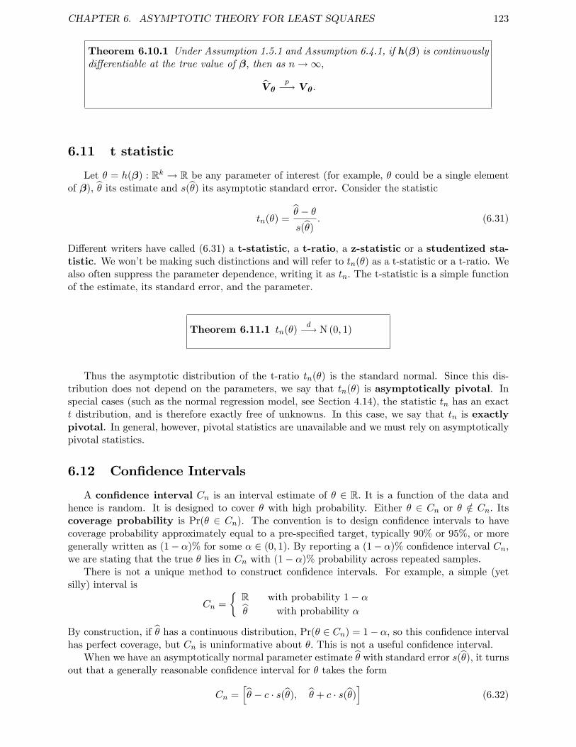
CHAPTER 6. ASYMPTOTIC THEORY FOR LEAST SQUARES 123
Theorem 6.10.1 Under Assumption 1.5.1 and Assumption 6.4.1, if h(β) is continuouslydifferentiable at the true value of β, then as n→∞,
V θp−→ V θ.
6.11 t statistic
Let θ = h(β) : Rk → R be any parameter of interest (for example, θ could be a single elementof β), θ its estimate and s(θ) its asymptotic standard error. Consider the statistic
tn(θ) =θ − θs(θ)
. (6.31)
Different writers have called (6.31) a t-statistic, a t-ratio, a z-statistic or a studentized sta-tistic. We won’t be making such distinctions and will refer to tn(θ) as a t-statistic or a t-ratio. Wealso often suppress the parameter dependence, writing it as tn. The t-statistic is a simple functionof the estimate, its standard error, and the parameter.
Theorem 6.11.1 tn(θ)d−→ N (0, 1)
Thus the asymptotic distribution of the t-ratio tn(θ) is the standard normal. Since this dis-tribution does not depend on the parameters, we say that tn(θ) is asymptotically pivotal. Inspecial cases (such as the normal regression model, see Section 4.14), the statistic tn has an exactt distribution, and is therefore exactly free of unknowns. In this case, we say that tn is exactlypivotal. In general, however, pivotal statistics are unavailable and we must rely on asymptoticallypivotal statistics.
6.12 Confidence Intervals
A confidence interval Cn is an interval estimate of θ ∈ R. It is a function of the data andhence is random. It is designed to cover θ with high probability. Either θ ∈ Cn or θ /∈ Cn. Itscoverage probability is Pr(θ ∈ Cn). The convention is to design confidence intervals to havecoverage probability approximately equal to a pre-specified target, typically 90% or 95%, or moregenerally written as (1− α)% for some α ∈ (0, 1). By reporting a (1− α)% confidence interval Cn,we are stating that the true θ lies in Cn with (1− α)% probability across repeated samples.
There is not a unique method to construct confidence intervals. For example, a simple (yetsilly) interval is
Cn =
R with probability 1− αθ with probability α
By construction, if θ has a continuous distribution, Pr(θ ∈ Cn) = 1− α, so this confidence intervalhas perfect coverage, but Cn is uninformative about θ. This is not a useful confidence interval.
When we have an asymptotically normal parameter estimate θ with standard error s(θ), it turnsout that a generally reasonable confidence interval for θ takes the form
Cn =[θ − c · s(θ), θ + c · s(θ)
](6.32)
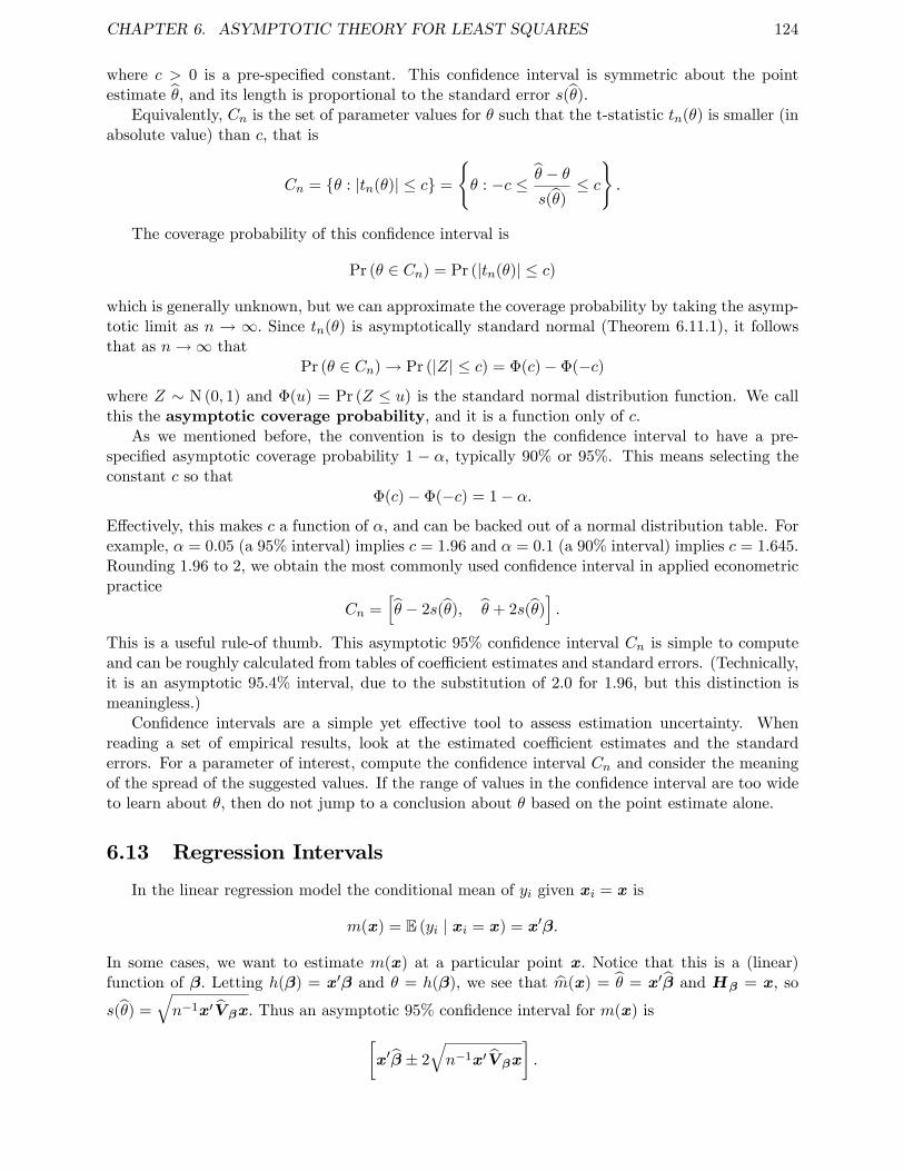
CHAPTER 6. ASYMPTOTIC THEORY FOR LEAST SQUARES 124
where c > 0 is a pre-specified constant. This confidence interval is symmetric about the pointestimate θ, and its length is proportional to the standard error s(θ).
Equivalently, Cn is the set of parameter values for θ such that the t-statistic tn(θ) is smaller (inabsolute value) than c, that is
Cn = θ : |tn(θ)| ≤ c =
θ : −c ≤ θ − θ
s(θ)≤ c.
The coverage probability of this confidence interval is
Pr (θ ∈ Cn) = Pr (|tn(θ)| ≤ c)
which is generally unknown, but we can approximate the coverage probability by taking the asymp-totic limit as n → ∞. Since tn(θ) is asymptotically standard normal (Theorem 6.11.1), it followsthat as n→∞ that
Pr (θ ∈ Cn)→ Pr (|Z| ≤ c) = Φ(c)− Φ(−c)
where Z ∼ N (0, 1) and Φ(u) = Pr (Z ≤ u) is the standard normal distribution function. We callthis the asymptotic coverage probability, and it is a function only of c.
As we mentioned before, the convention is to design the confidence interval to have a pre-specified asymptotic coverage probability 1 − α, typically 90% or 95%. This means selecting theconstant c so that
Φ(c)− Φ(−c) = 1− α.
Effectively, this makes c a function of α, and can be backed out of a normal distribution table. Forexample, α = 0.05 (a 95% interval) implies c = 1.96 and α = 0.1 (a 90% interval) implies c = 1.645.Rounding 1.96 to 2, we obtain the most commonly used confidence interval in applied econometricpractice
Cn =[θ − 2s(θ), θ + 2s(θ)
].
This is a useful rule-of thumb. This asymptotic 95% confidence interval Cn is simple to computeand can be roughly calculated from tables of coeffi cient estimates and standard errors. (Technically,it is an asymptotic 95.4% interval, due to the substitution of 2.0 for 1.96, but this distinction ismeaningless.)
Confidence intervals are a simple yet effective tool to assess estimation uncertainty. Whenreading a set of empirical results, look at the estimated coeffi cient estimates and the standarderrors. For a parameter of interest, compute the confidence interval Cn and consider the meaningof the spread of the suggested values. If the range of values in the confidence interval are too wideto learn about θ, then do not jump to a conclusion about θ based on the point estimate alone.
6.13 Regression Intervals
In the linear regression model the conditional mean of yi given xi = x is
m(x) = E (yi | xi = x) = x′β.
In some cases, we want to estimate m(x) at a particular point x. Notice that this is a (linear)function of β. Letting h(β) = x′β and θ = h(β), we see that m(x) = θ = x′β and Hβ = x, so
s(θ) =√n−1x′V βx. Thus an asymptotic 95% confidence interval for m(x) is[
x′β ± 2
√n−1x′V βx
].
CHAPTER 6. ASYMPTOTIC THEORY FOR LEAST SQUARES 125
Figure 6.7: Wage on Education Regression Intervals
It is interesting to observe that if this is viewed as a function of x, the width of the confidence setis dependent on x.
To illustrate, we return to the log wage regression (4.9) of Section 4.4. The estimated regressionequation is
log(Wage) = x′β = 0.626 + 0.156x.
where x = Education. The White covariance matrix estimate is
Vβ
=
(7.092 −0.445−0.445 0.029
)and the sample size is n = 61. Thus the 95% confidence interval for the regression takes the form
0.626 + 0.156x± 2
√1
61(7.092− 0.89x+ 0.029x2) .
The estimated regression and 95% intervals are shown in Figure 6.7. Notice that the confidencebands take a hyperbolic shape. This means that the regression line is less precisely estimated forvery large and very small values of education.
Plots of the estimated regression line and confidence intervals are especially useful when theregression includes nonlinear terms. To illustrate, consider the log wage regression (4.10) whichincludes experience and its square.
log(Wage) = 1.06 + 0.116 education+ 0.010 experience− 0.014 experience2/100 (6.33)
and has n = 2454 observations. We are interested in plotting the regression estimate and regressionintervals as a function of experience. Since the regression also includes education, in order to plotthe estimates in a simple graph we need to fix education at a specific value. We select education=12.This only affects the level of the estimated regression, since education enters without an interaction.Define the points of evaluation
x =
112x
x2/100
CHAPTER 6. ASYMPTOTIC THEORY FOR LEAST SQUARES 126
Figure 6.8: Wage on Experience Regression Intervals
where x =experience. The covariance matrix estimate is
Vβ
=
22.92 −1.0601 −0.56687 0.86626−1.0601 0.06454 .0080737 −.0066749−0.56687 .0080737 .040736 −.0755830.86626 −.0066749 −.075583 0.14994
.
Thus the regression interval for education=12, as a function of x =experience is
1.06 + 0.116 ∗ 12 + 0.010 x− 0.014 x2/100
± 1
50
√√√√√√√ 1
2454
(1 12 x x2/100
)22.92 −1.0601 −0.56687 0.86626−1.0601 0.06454 .0080737 −.0066749−0.56687 .0080737 .040736 −.0755830.86626 −.0066749 −.075583 0.14994
112x
x2/100
= 2.452 + 0.010 x− .00014 x2 ± 2
100
√27.592− 3.8304 x+ 0.23007 x2 − 0.00616 x3 + 0.0000611 x4
The estimated regression and 95% intervals are shown in Figure 6.8. The regression intervalwidens greatly for small and large values of experience, indicating considerable uncertainty aboutthe effect of experience on mean wages for this population. The confidence bands take a morecomplicated shape than in Figure 6.7 due to the nonlinear specification.
6.14 Quadratic Forms
Let θ = h(β) : Rk → Rq be any parameter vector of interest, θ its estimate and V θ itscovariance matrix estimator. Consider the quadratic form
Wn(θ) = n(θ − θ
)′V−1
θ
(θ − θ
). (6.34)
When q = 1 then Wn(θ) = tn(θ)2 is the square of the t-ratio. When q > 1 Wn(θ) is typically calledaWald statistic. We are interested in its sampling distribution.
CHAPTER 6. ASYMPTOTIC THEORY FOR LEAST SQUARES 127
The asymptotic distribution of Wn(θ) is simple to derive given Theorem 6.9.2 and Theorem6.10.1, which show that √
n(θ − θ
)d−→ Z ∼ N (0,V θ)
andV θ
p−→ V θ.
It follows thatWn(θ) =
√n(θ − θ
)′V−1
θ
√n(θ − θ
)d−→ Z′V −1
θ Z (6.35)
a quadratic in the normal random vector Z. Here we can appeal to a useful result from probabilitytheory. (See Theorem B.9.3 in the Appendix.)
Theorem 6.14.1 If Z ∼ N (0,A) with A > 0, q × q, then Z ′A−1Z ∼ χ2q , a chi-square
random variable with q degrees of freedom.
The asymptotic distribution in (6.35) takes exactly this form. It follows that Wn(θ) convergesin distribution to a chi-square random variable.
Theorem 6.14.2 Under Assumption 1.5.1 and Assumption 6.4.1, if h(β) is continuouslydifferentiable at the true value of β, then as n→∞,
Wn(θ)d−→ χ2
q .
6.15 Confidence Regions
A confidence region Cn is a generalization of a confidence interval to the case θ ∈ Rq with q > 1.A confidence region Cn is a set in Rq intended to cover the true parameter value with a pre-selectedprobability 1−α. Thus an ideal confidence region has the coverage probability Pr(θ ∈ Cn) = 1−α.In practice it is typically not possible to construct a region with exact coverage, but we can calculateits asymptotic coverage.
When the parameter estimate satisfies the conditions of Theorem 6.14.2, a good choice for aconfidence region is the ellipse
Cn = θ : Wn(θ) ≤ c1−α .
with c1−α the 1 − α’th quantile of the χ2q distribution. (Thus Fq(c1−α) = 1 − α.) These quantiles
can be found from a critical value table for the χ2q distribution.
Theorem 6.14.2 implies
Pr (θ ∈ Cn)→ Pr(χ2q ≤ c1−α
)= 1− α
which shows that Cn has asymptotic coverage (1− α)%.To illustrate the construction of a confidence region, consider the estimated regression (6.33) of
the model
log(Wage) = α+ β1 education+ β2 experience+ β3 experience2/100.
CHAPTER 6. ASYMPTOTIC THEORY FOR LEAST SQUARES 128
Suppose that the two parameters of interest are the percentage return to education θ1 = 100β1 andthe percentage return to experience for individuals with 10 years experience θ2 = 100β2 + 20β3.(We need to condition on the level of experience since the regression is quadratic in experience.)These two parameters are a linear transformation of the regression parameters with point estimates
θ =
(0 100 0 00 0 100 20
)β =
(11.60.72
),
and have the covariance matrix estimate
V θ =
(0 100 0 00 0 100 20
)Vβ
0 0
100 00 1000 20
=
(645.4 67.38767.387 165
)with inverse
V−1
θ =
(0.0016184 −0.00066098−0.00066098 0.0063306
).
Thus the Wald statistic is
Wn(θ) = n(θ − θ
)′V−1
θ
(θ − θ
)= 2454
(11.6− θ1
0.72− θ2
)′(0.0016184 −0.00066098−0.00066098 0.0063306
)(11.6− θ1
0.72− θ2
)= 3.97 (11.6− θ1)2 − 3.2441 (11.6− θ1) (0.72− θ2) + 15.535 (0.72− θ2)2
The 90% quantile of the χ22 distribution is 4.605 (we use the χ
22 distribution as the dimension
of θ is two), so an asymptotic 90% confidence region for the two parameters is the interior of theellipse
3.97 (11.6− θ1)2 − 3.2441 (11.6− θ1) (0.72− θ2) + 15.535 (0.72− θ2)2 = 4.605
which is displayed in Figure 6.9. Since the estimated correlation of the two coeffi cient estimates issmall (about 0.2) the ellipse is close to circular.
6.16 Semiparametric Effi ciency in the Projection Model
In Section 5.4 we presented the Gauss-Markov theorem, which stated that in the homoskedasticCEF model, in the class of linear unbiased estimators the one with the smallest variance is least-squares. As we noted in that section, the restriction to linear unbiased estimators is unsatisfactoryas it leaves open the possibility that an alternative (non-linear) estimator could have a smallerasymptotic variance. In addition, the restriction to the homoskedastic CEF model is also unsatis-factory as the projection model is more relevant for empirical application. The question remains:what is the most effi cient estimator of the projection coeffi cient β (or functions θ = h(β)) in theprojection model?
It turns out that it is straightforward to show that the projection model falls in the estimatorclass considered in Proposition 2.13.2. It follows that the least-squares estimator is semiparametri-cally effi cient in the sense that it has the smallest asymptotic variance in the class of semiparametricestimators of β. This is a more powerful and interesting result than the Gauss-Markov theorem.
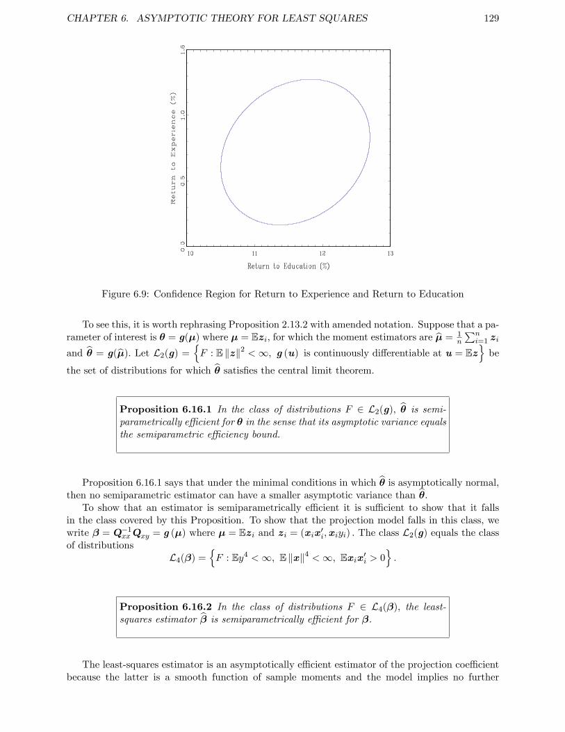
CHAPTER 6. ASYMPTOTIC THEORY FOR LEAST SQUARES 129
Figure 6.9: Confidence Region for Return to Experience and Return to Education
To see this, it is worth rephrasing Proposition 2.13.2 with amended notation. Suppose that a pa-rameter of interest is θ = g(µ) where µ = Ezi, for which the moment estimators are µ = 1
n
∑ni=1 zi
and θ = g(µ). Let L2(g) =F : E ‖z‖2 <∞, g (u) is continuously differentiable at u = Ez
be
the set of distributions for which θ satisfies the central limit theorem.
Proposition 6.16.1 In the class of distributions F ∈ L2(g), θ is semi-parametrically effi cient for θ in the sense that its asymptotic variance equalsthe semiparametric effi ciency bound.
Proposition 6.16.1 says that under the minimal conditions in which θ is asymptotically normal,then no semiparametric estimator can have a smaller asymptotic variance than θ.
To show that an estimator is semiparametrically effi cient it is suffi cient to show that it fallsin the class covered by this Proposition. To show that the projection model falls in this class, wewrite β = Q−1
xxQxy = g (µ) where µ = Ezi and zi = (xix′i,xiyi) . The class L2(g) equals the class
of distributionsL4(β) =
F : Ey4 <∞, E ‖x‖4 <∞, Exix′i > 0
.
Proposition 6.16.2 In the class of distributions F ∈ L4(β), the least-squares estimator β is semiparametrically effi cient for β.
The least-squares estimator is an asymptotically effi cient estimator of the projection coeffi cientbecause the latter is a smooth function of sample moments and the model implies no further
CHAPTER 6. ASYMPTOTIC THEORY FOR LEAST SQUARES 130
restrictions. However, if the class of permissible distributions is restricted to a strict subset of L4(β)then least-squares can be ineffi cient. For example, the linear CEF model with heteroskedastic errorsis a strict subset of L4(β), and the GLS estimator has a smaller asymptotic variance than OLS. Inthis case, the knowledge that true conditional mean is linear allows for more effi cient estimation ofthe unknown parameter.
From Proposition 6.16.1 we can also deduce that plug-in estimators θ = h(β) are semiparamet-rically effi cient estimators of θ = h(β) when h is continuously differentiable. We can also deducethat other parameters estimators are semiparametrically effi cient, such as σ2 for σ2. To see this,note that we can write
σ2 = E(yi − x′iβ
)2= Ey2
i − 2E(yix′i
)β + β′E
(xix
′i
)β
= Qyy −QyxQ−1xxQxy
which is a smooth function of the moments Qyy, Qyx and Qxx. Similarly the estimator σ2 equals
σ2 =1
n
n∑i=1
e2i
= Qyy − QyxQ−1
xxQxy
Since the variables y2i , yix
′i and xix
′i all have finite variances when F ∈ L4(β), the conditions of
Proposition 6.16.1 are satisfied. We conclude:
Proposition 6.16.3 In the class of distributions F ∈ L4(β), σ2 is semi-parametrically effi cient for σ2.
6.17 Semiparametric Effi ciency in the Homoskedastic RegressionModel*
In Section 6.16 we showed that the OLS estimator is semiparametrically effi cient in the projec-tion model. What if we restrict attention to the classical homoskedastic regression model? Is OLSstill effi cient in this class? In this section we derive the asymptotic semiparametric effi ciency boundfor this model, and show that it is the same as that obtained by the OLS estimator. Therefore itturns out that least-squares is effi cient in this class as well.
Recall that in the homoskedastic regression model the asymptotic variance of the OLS estimatorβ for β is V 0
β = Q−1xxσ
2. Therefore, as described in Section 2.13, it is suffi cient to find a parametricsubmodel whose Cramer-Rao bound for estimation of β is V 0
β. This would establish that V0β is
the semiparametric variance bound and the OLS estimator β is semiparametrically effi cient for β.Let the joint density of y and x be written as f (y,x) = f1 (y | x) f2 (x) , the product of the
conditional density of y given x and the marginal density of x. Now consider the parametricsubmodel
f (y,x | θ) = f1 (y | x)(1 +
(y − x′β
) (x′θ)/σ2)f2 (x) . (6.36)
You can check that in this submodel the marginal density of x is f2 (x) and the conditional densityof y given x is f1 (y | x)
(1 + (y − x′β) (x′θ) /σ2
). To see that the latter is a valid conditional
density, observe that the regression assumption implies that∫yf1 (y | x) dy = x′β and therefore∫
f1 (y | x)(1 +
(y − x′β
) (x′θ)/σ2)dy =
∫f1 (y | x) dy +
∫f1 (y | x)
(y − x′β
)dy(x′θ)/σ2
= 1.
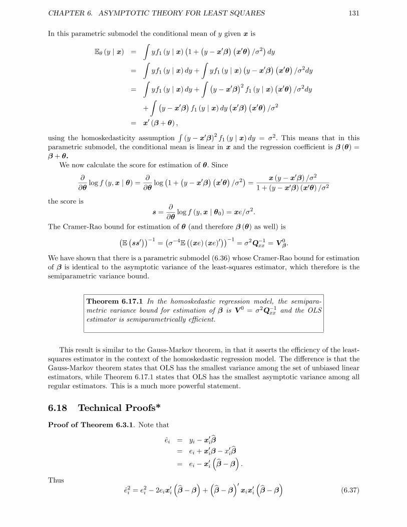
CHAPTER 6. ASYMPTOTIC THEORY FOR LEAST SQUARES 131
In this parametric submodel the conditional mean of y given x is
Eθ (y | x) =
∫yf1 (y | x)
(1 +
(y − x′β
) (x′θ)/σ2)dy
=
∫yf1 (y | x) dy +
∫yf1 (y | x)
(y − x′β
) (x′θ)/σ2dy
=
∫yf1 (y | x) dy +
∫ (y − x′β
)2f1 (y | x)
(x′θ)/σ2dy
+
∫ (y − x′β
)f1 (y | x) dy
(x′β
) (x′θ)/σ2
= x′ (β + θ) ,
using the homoskedasticity assumption∫
(y − x′β)2 f1 (y | x) dy = σ2. This means that in thisparametric submodel, the conditional mean is linear in x and the regression coeffi cient is β (θ) =β + θ.
We now calculate the score for estimation of θ. Since
∂
∂θlog f (y,x | θ) =
∂
∂θlog(1 +
(y − x′β
) (x′θ)/σ2)
=x (y − x′β) /σ2
1 + (y − x′β) (x′θ) /σ2
the score is
s =∂
∂θlog f (y,x | θ0) = xe/σ2.
The Cramer-Rao bound for estimation of θ (and therefore β (θ) as well) is(E(ss′))−1
=(σ−4E
((xe) (xe)′
))−1= σ2Q−1
xx = V 0β.
We have shown that there is a parametric submodel (6.36) whose Cramer-Rao bound for estimationof β is identical to the asymptotic variance of the least-squares estimator, which therefore is thesemiparametric variance bound.
Theorem 6.17.1 In the homoskedastic regression model, the semipara-metric variance bound for estimation of β is V 0 = σ2Q−1
xx and the OLSestimator is semiparametrically effi cient.
This result is similar to the Gauss-Markov theorem, in that it asserts the effi ciency of the least-squares estimator in the context of the homoskedastic regression model. The difference is that theGauss-Markov theorem states that OLS has the smallest variance among the set of unbiased linearestimators, while Theorem 6.17.1 states that OLS has the smallest asymptotic variance among allregular estimators. This is a much more powerful statement.
6.18 Technical Proofs*
Proof of Theorem 6.3.1. Note that
ei = yi − x′iβ= ei + x′iβ − x′iβ= ei − x′i
(β − β
).
Thuse2i = e2
i − 2eix′i
(β − β
)+(β − β
)′xix
′i
(β − β
)(6.37)
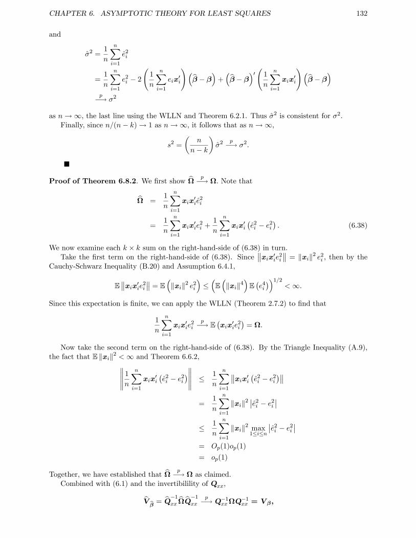
CHAPTER 6. ASYMPTOTIC THEORY FOR LEAST SQUARES 132
and
σ2 =1
n
n∑i=1
e2i
=1
n
n∑i=1
e2i − 2
(1
n
n∑i=1
eix′i
)(β − β
)+(β − β
)′( 1
n
n∑i=1
xix′i
)(β − β
)p−→ σ2
as n→∞, the last line using the WLLN and Theorem 6.2.1. Thus σ2 is consistent for σ2.Finally, since n/(n− k)→ 1 as n→∞, it follows that as n→∞,
s2 =
(n
n− k
)σ2 p−→ σ2.
Proof of Theorem 6.8.2. We first show Ωp−→ Ω. Note that
Ω =1
n
n∑i=1
xix′ie
2i
=1
n
n∑i=1
xix′ie
2i +
1
n
n∑i=1
xix′i
(e2i − e2
i
). (6.38)
We now examine each k × k sum on the right-hand-side of (6.38) in turn.Take the first term on the right-hand-side of (6.38). Since
∥∥xix′ie2i
∥∥ = ‖xi‖2 e2i , then by the
Cauchy-Schwarz Inequality (B.20) and Assumption 6.4.1,
E∥∥xix′ie2
i
∥∥ = E(‖xi‖2 e2
i
)≤(E(‖xi‖4
)E(e4i
))1/2<∞.
Since this expectation is finite, we can apply the WLLN (Theorem 2.7.2) to find that
1
n
n∑i=1
xix′ie
2i
p−→ E(xix
′ie
2i
)= Ω.
Now take the second term on the right-hand-side of (6.38). By the Triangle Inequality (A.9),the fact that E ‖xi‖2 <∞ and Theorem 6.6.2,∥∥∥∥∥ 1
n
n∑i=1
xix′i
(e2i − e2
i
)∥∥∥∥∥ ≤ 1
n
n∑i=1
∥∥xix′i (e2i − e2
i
)∥∥=
1
n
n∑i=1
‖xi‖2∣∣e2i − e2
i
∣∣≤ 1
n
n∑i=1
‖xi‖2 max1≤i≤n
∣∣e2i − e2
i
∣∣= Op(1)op(1)
= op(1)
Together, we have established that Ωp−→ Ω as claimed.
Combined with (6.1) and the invertibilility of Qxx,
Vβ
= Q−1
xx ΩQ−1
xxp−→ Q−1
xxΩQ−1xx = V β,
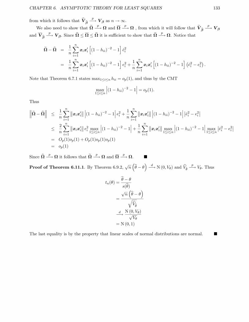
CHAPTER 6. ASYMPTOTIC THEORY FOR LEAST SQUARES 133
from which it follows that Vβ
p−→ V β as n→∞.We also need to show that Ω
p−→ Ω and Ωp−→ Ω , from which it will follow that V
β
p−→ V β
and Vβ
p−→ V β. Since Ω ≤ Ω ≤ Ω it is suffi cient to show that Ωp−→ Ω. Notice that
Ω− Ω =1
n
n∑i=1
xix′i
[(1− hii)−2 − 1
]e2i
=1
n
n∑i=1
xix′i
[(1− hii)−2 − 1
]e2i +
1
n
n∑i=1
xix′i
[(1− hii)−2 − 1
] (e2i − e2
i
).
Note that Theorem 6.7.1 states max1≤i≤n hii = op(1), and thus by the CMT
max1≤i≤n
∣∣∣(1− hii)−2 − 1∣∣∣ = op(1).
Thus∥∥∥Ω− Ω∥∥∥ ≤ 1
n
n∑i=1
∥∥xix′i∥∥ ∣∣∣(1− hii)−2 − 1∣∣∣ e2i +
1
n
n∑i=1
∥∥xix′i∥∥ ∣∣∣(1− hii)−2 − 1∣∣∣ ∣∣e2
i − e2i
∣∣≤ 2
n
n∑i=1
∥∥xix′i∥∥ e2i max
1≤i≤n
∣∣∣(1− hii)−2 − 1∣∣∣+
1
n
n∑i=1
∥∥xix′i∥∥ max1≤i≤n
∣∣∣(1− hii)−2 − 1∣∣∣ max
1≤i≤n
∣∣e2i − e2
i
∣∣= Op(1)op(1) +Op(1)op(1)op(1)
= op(1)
Since Ωp−→ Ω it follows that Ω
p−→ Ω and Ωp−→ Ω.
Proof of Theorem 6.11.1. By Theorem 6.9.2,√n(θ − θ
)d−→ N (0, Vθ) and Vθ
p−→ Vθ. Thus
tn(θ) =θ − θs(θ)
=
√n(θ − θ
)√Vθ
d−→ N (0, Vθ)√Vθ
= N (0, 1)
The last equality is by the property that linear scales of normal distributions are normal.
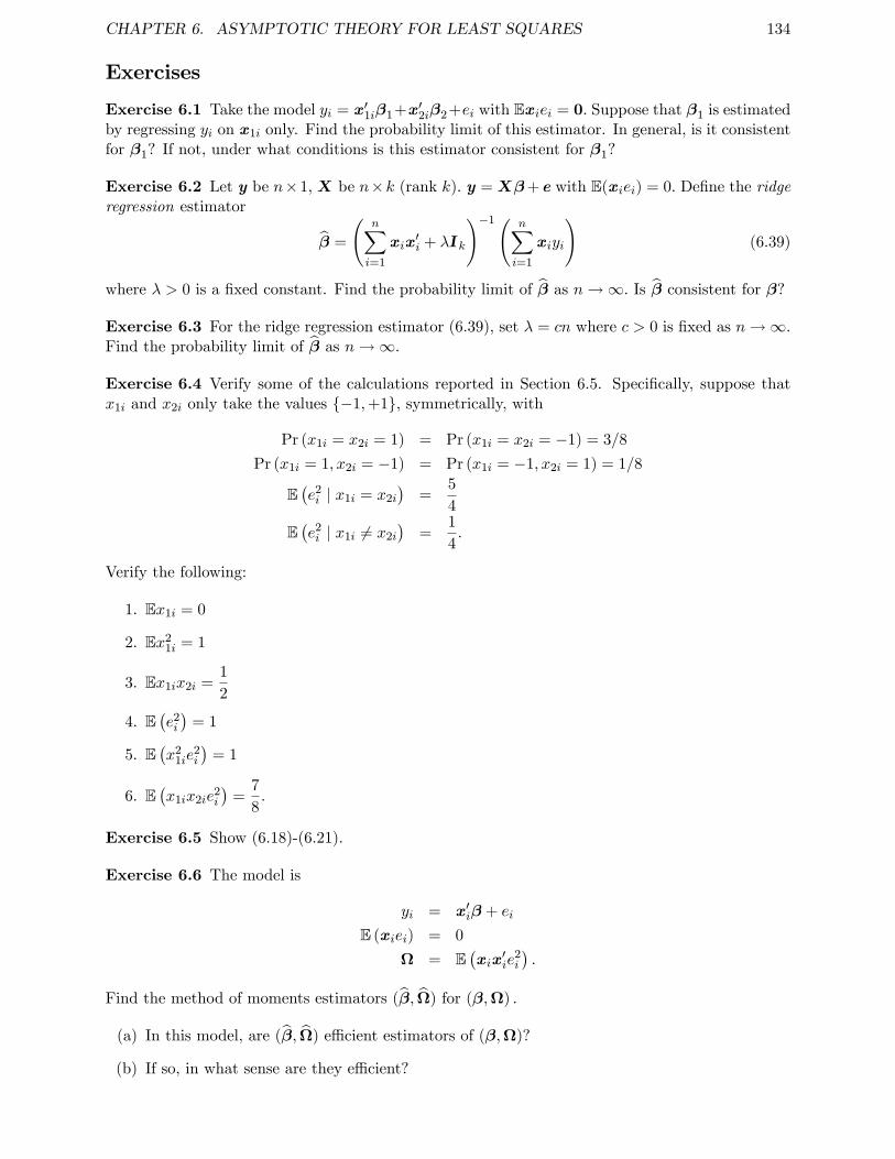
CHAPTER 6. ASYMPTOTIC THEORY FOR LEAST SQUARES 134
Exercises
Exercise 6.1 Take the model yi = x′1iβ1+x′2iβ2+ei with Exiei = 0. Suppose that β1 is estimatedby regressing yi on x1i only. Find the probability limit of this estimator. In general, is it consistentfor β1? If not, under what conditions is this estimator consistent for β1?
Exercise 6.2 Let y be n×1, X be n×k (rank k). y = Xβ+e with E(xiei) = 0. Define the ridgeregression estimator
β =
(n∑i=1
xix′i + λIk
)−1( n∑i=1
xiyi
)(6.39)
where λ > 0 is a fixed constant. Find the probability limit of β as n→∞. Is β consistent for β?
Exercise 6.3 For the ridge regression estimator (6.39), set λ = cn where c > 0 is fixed as n→∞.Find the probability limit of β as n→∞.
Exercise 6.4 Verify some of the calculations reported in Section 6.5. Specifically, suppose thatx1i and x2i only take the values −1,+1, symmetrically, with
Pr (x1i = x2i = 1) = Pr (x1i = x2i = −1) = 3/8
Pr (x1i = 1, x2i = −1) = Pr (x1i = −1, x2i = 1) = 1/8
E(e2i | x1i = x2i
)=
5
4
E(e2i | x1i 6= x2i
)=
1
4.
Verify the following:
1. Ex1i = 0
2. Ex21i = 1
3. Ex1ix2i =1
2
4. E(e2i
)= 1
5. E(x2
1ie2i
)= 1
6. E(x1ix2ie
2i
)=
7
8.
Exercise 6.5 Show (6.18)-(6.21).
Exercise 6.6 The model is
yi = x′iβ + ei
E (xiei) = 0
Ω = E(xix
′ie
2i
).
Find the method of moments estimators (β, Ω) for (β,Ω) .
(a) In this model, are (β, Ω) effi cient estimators of (β,Ω)?
(b) If so, in what sense are they effi cient?
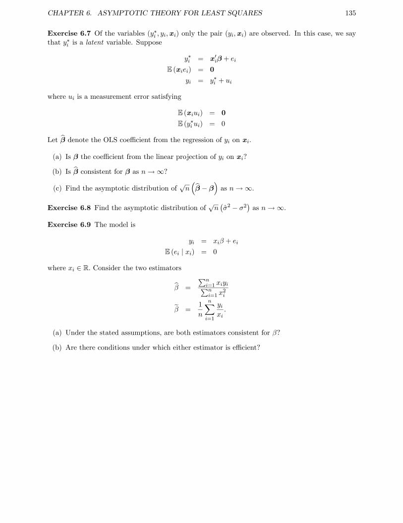
CHAPTER 6. ASYMPTOTIC THEORY FOR LEAST SQUARES 135
Exercise 6.7 Of the variables (y∗i , yi,xi) only the pair (yi,xi) are observed. In this case, we saythat y∗i is a latent variable. Suppose
y∗i = x′iβ + ei
E (xiei) = 0
yi = y∗i + ui
where ui is a measurement error satisfying
E (xiui) = 0
E (y∗i ui) = 0
Let β denote the OLS coeffi cient from the regression of yi on xi.
(a) Is β the coeffi cient from the linear projection of yi on xi?
(b) Is β consistent for β as n→∞?
(c) Find the asymptotic distribution of√n(β − β
)as n→∞.
Exercise 6.8 Find the asymptotic distribution of√n(σ2 − σ2
)as n→∞.
Exercise 6.9 The model is
yi = xiβ + ei
E (ei | xi) = 0
where xi ∈ R. Consider the two estimators
β =
∑ni=1 xiyi∑ni=1 x
2i
β =1
n
n∑i=1
yixi.
(a) Under the stated assumptions, are both estimators consistent for β?
(b) Are there conditions under which either estimator is effi cient?
Chapter 7
Restricted Estimation
7.1 Introduction
In the linear projection model
yi = x′iβ + ei
E (xiei) = 0
a common task is to impose a constraint on the coeffi cient vector β. For example, partitioningx′i = (x′1i,x
′2i) and β
′ =(β′1,β
′2
), a typical constraint is an exclusion restriction of the form
β2 = 0. In this case the constrained model is
yi = x′1iβ1 + ei
E (xiei) = 0
At first glance this appears the same as the linear projection model, but there is one importantdifference: the error ei is uncorrelated with the entire regressor vector x′i = (x′1i,x
′2i) not just the
included regressor x1i.In general, a set of q linear constraints on β takes the form
R′β = c (7.1)
where R is k × q, rank(R) = q < k and c is q × 1. The assumption that R is full rank means thatthe constraints are linearly independent (there are no redundant or contradictory constraints).
The constraint β2 = 0 discussed above is a special case of the constraint (7.1) with
R =
(0I
), (7.2)
a selector matrix, and c = 0.Another common restriction is that a set of coeffi cients sum to a known constant, i.e. β1+β2 = 1.
This constraint arises in a constant-return-to-scale production function. Other common restrictionsinclude the equality of coeffi cients β1 = β2, and equal and offsetting coeffi cients β1 − β2 = 0.
A typical reason to impose a constraint is that we believe (or have information) that the con-straint is true. By imposing the constraint we hope to improve estimation effi ciency. The goal isto obtain consistent estimates with reduced variance relative to the unconstrained estimator.
The questions then arise: How should we estimate the coeffi cient vector β imposing the linearrestriction (7.1)? If we impose such constraints, what is the sampling distribution of the resultingestimator? How should we calculate standard errors? These are the questions explored in thischapter.
136
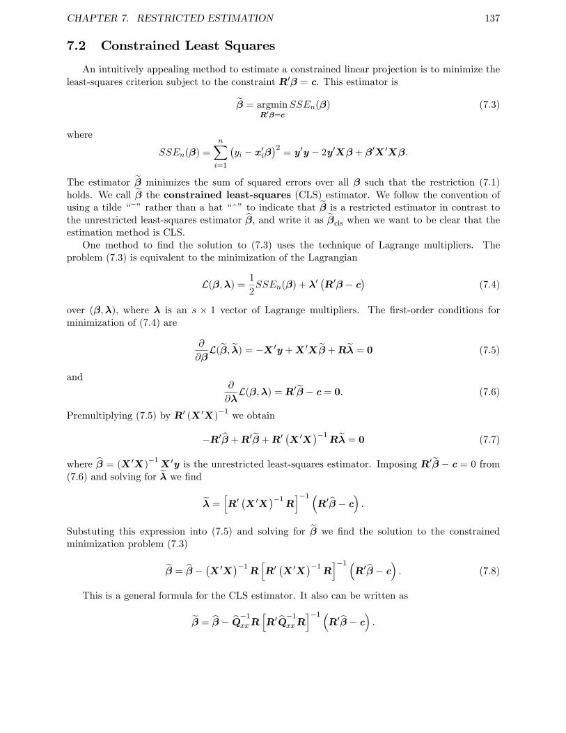
CHAPTER 7. RESTRICTED ESTIMATION 137
7.2 Constrained Least Squares
An intuitively appealing method to estimate a constrained linear projection is to minimize theleast-squares criterion subject to the constraint R′β = c. This estimator is
β = argminR′β=c
SSEn(β) (7.3)
where
SSEn(β) =
n∑i=1
(yi − x′iβ
)2= y′y − 2y′Xβ + β′X ′Xβ.
The estimator β minimizes the sum of squared errors over all β such that the restriction (7.1)holds. We call β the constrained least-squares (CLS) estimator. We follow the convention ofusing a tilde “~”rather than a hat “^”to indicate that β is a restricted estimator in contrast tothe unrestricted least-squares estimator β, and write it as βcls when we want to be clear that theestimation method is CLS.
One method to find the solution to (7.3) uses the technique of Lagrange multipliers. Theproblem (7.3) is equivalent to the minimization of the Lagrangian
L(β,λ) =1
2SSEn(β) + λ′
(R′β − c
)(7.4)
over (β,λ), where λ is an s × 1 vector of Lagrange multipliers. The first-order conditions forminimization of (7.4) are
∂
∂βL(β, λ) = −X ′y +X ′Xβ +Rλ = 0 (7.5)
and∂
∂λL(β,λ) = R′β − c = 0. (7.6)
Premultiplying (7.5) by R′ (X ′X)−1 we obtain
−R′β +R′β +R′(X ′X
)−1Rλ = 0 (7.7)
where β = (X ′X)−1X ′y is the unrestricted least-squares estimator. Imposing R′β − c = 0 from
(7.6) and solving for λ we find
λ =[R′(X ′X
)−1R]−1 (
R′β − c).
Substuting this expression into (7.5) and solving for β we find the solution to the constrainedminimization problem (7.3)
β = β −(X ′X
)−1R[R′(X ′X
)−1R]−1 (
R′β − c). (7.8)
This is a general formula for the CLS estimator. It also can be written as
β = β − Q−1
xxR[R′Q
−1
xxR]−1 (
R′β − c).
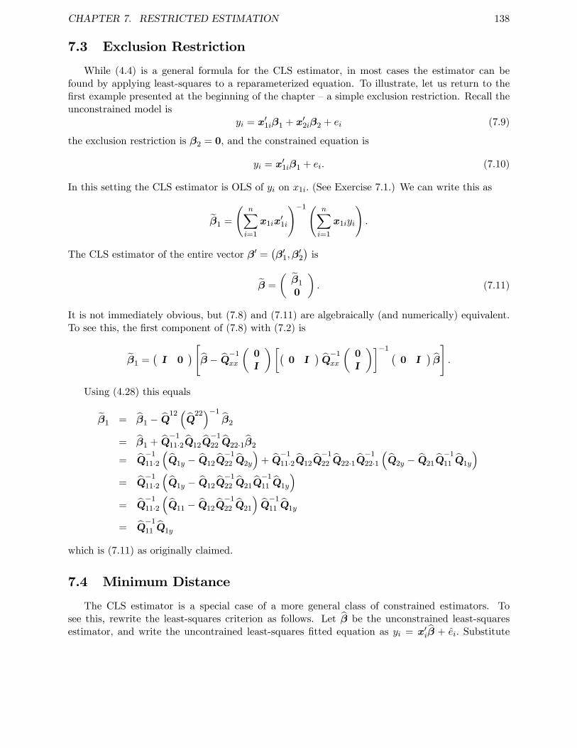
CHAPTER 7. RESTRICTED ESTIMATION 138
7.3 Exclusion Restriction
While (4.4) is a general formula for the CLS estimator, in most cases the estimator can befound by applying least-squares to a reparameterized equation. To illustrate, let us return to thefirst example presented at the beginning of the chapter —a simple exclusion restriction. Recall theunconstrained model is
yi = x′1iβ1 + x′2iβ2 + ei (7.9)
the exclusion restriction is β2 = 0, and the constrained equation is
yi = x′1iβ1 + ei. (7.10)
In this setting the CLS estimator is OLS of yi on x1i. (See Exercise 7.1.) We can write this as
β1 =
(n∑i=1
x1ix′1i
)−1( n∑i=1
x1iyi
).
The CLS estimator of the entire vector β′ =(β′1,β
′2
)is
β =
(β1
0
). (7.11)
It is not immediately obvious, but (7.8) and (7.11) are algebraically (and numerically) equivalent.To see this, the first component of (7.8) with (7.2) is
β1 =(I 0
) [β − Q−1
xx
(0I
)[(0 I
)Q−1
xx
(0I
)]−1 (0 I
)β
].
Using (4.28) this equals
β1 = β1 − Q12(Q
22)−1
β2
= β1 + Q−1
11·2Q12Q−1
22 Q22·1β2
= Q−1
11·2
(Q1y − Q12Q
−1
22 Q2y
)+ Q
−1
11·2Q12Q−1
22 Q22·1Q−1
22·1
(Q2y − Q21Q
−1
11 Q1y
)= Q
−1
11·2
(Q1y − Q12Q
−1
22 Q21Q−1
11 Q1y
)= Q
−1
11·2
(Q11 − Q12Q
−1
22 Q21
)Q−1
11 Q1y
= Q−1
11 Q1y
which is (7.11) as originally claimed.
7.4 Minimum Distance
The CLS estimator is a special case of a more general class of constrained estimators. Tosee this, rewrite the least-squares criterion as follows. Let β be the unconstrained least-squaresestimator, and write the uncontrained least-squares fitted equation as yi = x′iβ + ei. Substitute
CHAPTER 7. RESTRICTED ESTIMATION 139
this equation into SSEn(β) to obtain
SSEn(β) =
n∑i=1
(yi − x′iβ
)2=
n∑i=1
(x′iβ + ei − x′iβ
)2
=n∑i=1
e2i +
(β − β
)′( n∑i=1
xix′i
)(β − β
)= nσ2 + n
(β − β
)′Qxx
(β − β
). (7.12)
where the third equality uses the fact that∑n
i=1 xiei = 0. Since the first term on the last line doesnot depend on β it follows that the CLS estimator minimizes the quadratic on the right-side of(7.12). This is a (squared) weighted Euclidean distance between β and β. It is a special case of thegeneral weighted distance
Jn (β,W n) = n(β − β
)′W−1
n
(β − β
)for W n > 0 a k × k positive definite weight matrix. In summary, we have found that the CLSestimator can be written as
β = argminR′β=c
Jn(β, Q−1
xx )
More generally, a minimum distance estimator for β is
βmd(W n) = argminR′β=c
Jn (β,W n) (7.13)
whereW n > 0. We have written the estimator as βmd(W n) as it depends upon the weight matrixW n.
An obvious question is which weight matrix W n is appropriate. We will address this questionafter we derive the asymptotic distribution for a general weight matrix.
7.5 Computation
A general method to solve the algebraic problem (7.13) is by the method of Lagrange multipliers.The Lagrangian is
L(β,λ) =1
2Jn (β,W n) + λ′
(R′β − c
)which is minimized over (β,λ). The solution is
βmd(W n) = β −W nR(R′W nR
)−1(R′β − c
). (7.14)
(See Exercise 7.5.)
If we set W n = Q−1
xx then (7.14) specializes to the CLS estimator:
βmd(Q−1
xx ) = βcls
In this sense the minimum distance estimator generalizes constrained least-squares.
CHAPTER 7. RESTRICTED ESTIMATION 140
7.6 Asymptotic Distribution
We first show that the class of minimum distance estimators are consistent for the populationparameters when the constraints are valid.
Assumption 7.6.1 R′β = c where R is k × q with rank(R) = q.
Theorem 7.6.1 ConsistencyUnder Assumption 1.5.1, Assumption 3.16.1, Assumption 7.6.1,and W n
p−→W > 0, βmd(W n)p−→ β as n→∞.
Theorem 7.6.1 shows that consistency holds for any weight matrix, so the result includes theCLS estimator.
Similarly, the constrained estimators are asymptotically normally distributed.
Theorem 7.6.2 Asymptotic NormalityUnder Assumption 1.5.1, Assumption 6.4.1, Assumption 7.6.1, and W n
p−→W > 0,
√n(βmd(W n)− β
)d−→ N (0,V β(W )) (7.15)
as n→∞, where
V β(W ) = V β −WR(R′WR
)−1R′V β − V βR
(R′WR
)−1R′W
+WR(R′WR
)−1R′V βR
(R′WR
)−1R′W (7.16)
andV β = Q−1
xxΩQ−1xx .
Theorem 7.6.2 shows that the minimum distance estimator is asymptotically normal for allpositive definite weight matrices. The asymptotic variance depends on W . The theorem includesthe CLS estimator as a special case by setting W = Q−1
xx .
Theorem 7.6.3 Asymptotic Distribution of CLS EstimatorUnder Assumption 1.5.1, Assumption 6.4.1, and Assumption 7.6.1, as n→∞
√n(βcls − β
)d−→ N (0,V cls)
where
V cls = V β −Q−1xxR
(R′Q−1
xxR)−1
R′V β − V βR(R′Q−1
xxR)−1
R′Q−1xx
+Q−1xxR
(R′Q−1
xxR)−1
R′V βR(R′Q−1
xxR)−1
R′Q−1xx
CHAPTER 7. RESTRICTED ESTIMATION 141
7.7 Effi cient Minimum Distance Estimator
Theorem 7.6.2 shows that the minimum distance estimators, which include CLS as a specialcase, are asymptotically normal with an asymptotic covariance matrix which depends on the weightmatrix W . The asymptotically optimal weight matrix is the one which minimizes the asymptoticvariance V β(W ). This turns out to be W = V β has shown in Theorem 7.7.1 below. Since V β isunknown this weight matrix cannot be used for a feasible estimator, but we can replace V β witha consistent estimate V β and the asymptotic distribution (and effi ciency) are unchanged. We callthe minimum distance estimator settingW n = V β the effi cient minimum distance estimatorand takes the form
β = β − V βR(R′V βR
)−1 (R′β − c
)(7.17)
This estimator has the smallest asymptotic variance in the class of minimum distance estimators,The asymptotic distribution of (7.17) can be deduced from Theorem 7.6.2.
Theorem 7.7.1 Effi cient Minimum Distance EstimatorUnder Assumption 1.5.1, Assumption 6.4.1, and Assumption 7.6.1, for β definedin (7.17) ,
√n(β − β
)d−→ N
(0,V ∗β
)as n→∞, where
V ∗β = V β − V βR(R′V βR
)−1R′V β. (7.18)
SinceV ∗β ≤ V β (7.19)
the estimator (7.17) has lower asymptotic variance than the unrestricted estimator.Furthermor, for any W ,
V ∗β ≤ V β(W ) (7.20)
so (7.17) is asymptotically effi cient in the class of minimum distance estimators.
Theorem 7.7.1 shows that the minimum distance estimator with the smallest asymptotic vari-ance is (7.17). One implication is that the constrained least squares estimator is generally inef-ficient. The interesting exception is the case of conditional homoskedasticity, in which case theoptimal weight matrix is W = V −1
β = σ−2Qxx so in this case CLS is an effi cient minimum dis-tance estimator. Otherwise when the error is conditionally heteroskedastic, there are asymptoticeffi ciency gains by using minimum distance rather than least squares.
The fact that CLS is generally ineffi cient is counter-intuitive and requires some reflection tounderstand. Standard intuition suggests to apply the same estimation method (least squares) tothe unconstrained and constrained models, and this is the most common empirical practice. Butour statistical analysis has shown that this is not the effi cient estimation method. Instead, theeffi cient minimum distance estimator has a smaller asymptotic variance. Why? The reason isthat the least-squares estimator does not make use of the regressor x2i. It ignores the informationE (x2iei) = 0. This information is relevant when the error is heteroskedastic and the excludedregressors are correlated with the included regressors.
Inequality (7.19) shows that the effi cient minimum distance estimator β has a smaller asymptoticvariance than the unrestricted least squares estimator β. This means that estimation is more effi cientby imposing correct restrictions when we use the minimum distance method.
CHAPTER 7. RESTRICTED ESTIMATION 142
7.8 Exclusion Restriction Revisited
We return to the example of estimation with a simple exclusion restriction. The model is
yi = x′1iβ1 + x′2iβ2 + ei
with the exclusion restriction β2 = 0. We have introduced three estimators of β1. The first isunconstrained least-squares applied to (7.9), which can be written as
β1 = Q−1
11·2Q1y·2.
From Theorem 6.28 and equation (6.19) its asymptotic variance is
avar(β1) = Q−111·2
(Ω11 −Q12Q
−122 Ω21 −Ω12Q
−122 Q21 +Q12Q
−122 Ω22Q
−122 Q21
)Q−1
11·2.
The second estimator of β1 is the CLS estimator, which can be written as
β1,cls = Q−1
11 Q1y.
Its asymptotic variance can be deduced from Theorem 7.6.3, but it is simpler to apply the CLTdirectly to show that
avar(β1,cls) = Q−111 Ω11Q
−111 . (7.21)
The third estimator of β1 is the effi cient minimum distance estimator. Applying (7.17), it equals
β1,md = β1 − V 12V−1
22 β2 (7.22)
where we have partitioned
V β =
[V 11 V 12
V 21 V 22
].
From Theorem 7.7.1 its asymptotic variance is
avar(β1,md) = V 11 − V 12V−122 V 21. (7.23)
In general, the three estimators are different, and they have different asymptotic variances.It is quite instructive to compare the asymptotic variances of the CLS and unconstrained least-
squares estimators to assess whether or not the constrained estimator is necessarily more effi cientthan the unconstrained estimator.
First, consider the case of conditional homoskedasticity. In this case the two covariance matricessimplify to
avar(β1) = σ2Q−111·2
andavar(β1,cls) = σ2Q−1
11 .
If Q12 = 0 (so x1i and x2i are orthogonal) then these two variance matrices equal and the twoestimators have equal asymptotic effi ciency. Otherwise, since Q12Q
−122 Q21 ≥ 0, then Q11 ≥ Q11 −
Q12Q−122 Q21, and consequently
Q−111 σ
2 ≤(Q11 −Q12Q
−122 Q21
)−1σ2.
This means that under conditional homoskedasticity, β1,cls has a lower asymptotic variance matrix
than β1. Therefore in this context, constrained least-squares is more effi cient than unconstrainedleast-squares. This is consistent with our intuition that imposing a correct restriction (excludingan irrelevant regressor) improves estimation effi ciency.
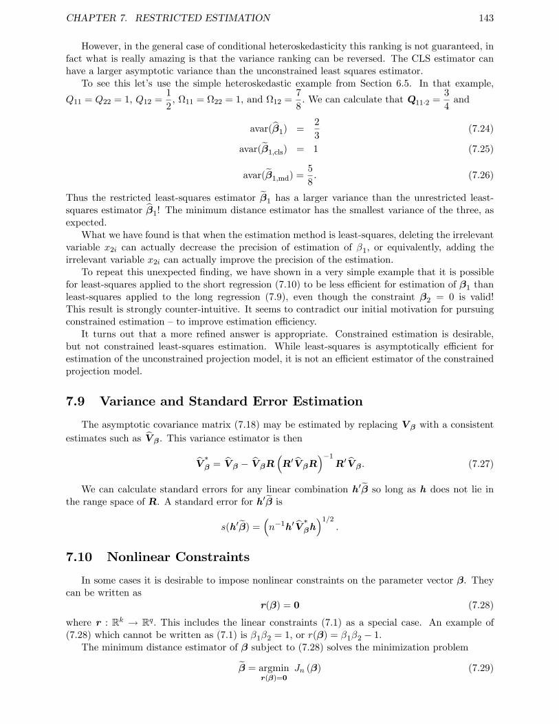
CHAPTER 7. RESTRICTED ESTIMATION 143
However, in the general case of conditional heteroskedasticity this ranking is not guaranteed, infact what is really amazing is that the variance ranking can be reversed. The CLS estimator canhave a larger asymptotic variance than the unconstrained least squares estimator.
To see this let’s use the simple heteroskedastic example from Section 6.5. In that example,
Q11 = Q22 = 1, Q12 =1
2, Ω11 = Ω22 = 1, and Ω12 =
7
8. We can calculate that Q11·2 =
3
4and
avar(β1) =2
3(7.24)
avar(β1,cls) = 1 (7.25)
avar(β1,md) =5
8. (7.26)
Thus the restricted least-squares estimator β1 has a larger variance than the unrestricted least-squares estimator β1! The minimum distance estimator has the smallest variance of the three, asexpected.
What we have found is that when the estimation method is least-squares, deleting the irrelevantvariable x2i can actually decrease the precision of estimation of β1, or equivalently, adding theirrelevant variable x2i can actually improve the precision of the estimation.
To repeat this unexpected finding, we have shown in a very simple example that it is possiblefor least-squares applied to the short regression (7.10) to be less effi cient for estimation of β1 thanleast-squares applied to the long regression (7.9), even though the constraint β2 = 0 is valid!This result is strongly counter-intuitive. It seems to contradict our initial motivation for pursuingconstrained estimation —to improve estimation effi ciency.
It turns out that a more refined answer is appropriate. Constrained estimation is desirable,but not constrained least-squares estimation. While least-squares is asymptotically effi cient forestimation of the unconstrained projection model, it is not an effi cient estimator of the constrainedprojection model.
7.9 Variance and Standard Error Estimation
The asymptotic covariance matrix (7.18) may be estimated by replacing V β with a consistentestimates such as V β. This variance estimator is then
V∗β = V β − V βR
(R′V βR
)−1R′V β. (7.27)
We can calculate standard errors for any linear combination h′β so long as h does not lie inthe range space of R. A standard error for h′β is
s(h′β) =(n−1h′V
∗βh)1/2
.
7.10 Nonlinear Constraints
In some cases it is desirable to impose nonlinear constraints on the parameter vector β. Theycan be written as
r(β) = 0 (7.28)
where r : Rk → Rq. This includes the linear constraints (7.1) as a special case. An example of(7.28) which cannot be written as (7.1) is β1β2 = 1, or r(β) = β1β2 − 1.
The minimum distance estimator of β subject to (7.28) solves the minimization problem
β = argminr(β)=0
Jn (β) (7.29)
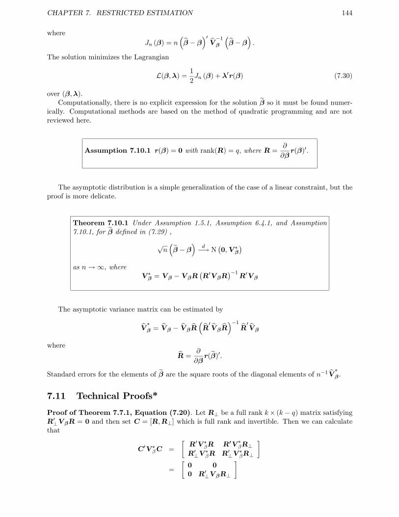
CHAPTER 7. RESTRICTED ESTIMATION 144
whereJn (β) = n
(β − β
)′V−1
β
(β − β
).
The solution minimizes the Lagrangian
L(β,λ) =1
2Jn (β) + λ′r(β) (7.30)
over (β,λ).Computationally, there is no explicit expression for the solution β so it must be found numer-
ically. Computational methods are based on the method of quadratic programming and are notreviewed here.
Assumption 7.10.1 r(β) = 0 with rank(R) = q, where R =∂
∂βr(β)′.
The asymptotic distribution is a simple generalization of the case of a linear constraint, but theproof is more delicate.
Theorem 7.10.1 Under Assumption 1.5.1, Assumption 6.4.1, and Assumption7.10.1, for β defined in (7.29) ,
√n(β − β
)d−→ N
(0,V ∗β
)as n→∞, where
V ∗β = V β − V βR(R′V βR
)−1R′V β
The asymptotic variance matrix can be estimated by
V∗β = V β − V βR
(R′V βR
)−1R′V β
where
R =∂
∂βr(β)′.
Standard errors for the elements of β are the square roots of the diagonal elements of n−1V∗β.
7.11 Technical Proofs*
Proof of Theorem 7.7.1, Equation (7.20). Let R⊥ be a full rank k× (k − q) matrix satisfyingR′⊥V βR = 0 and then set C = [R,R⊥] which is full rank and invertible. Then we can calculatethat
C ′V ∗βC =
[R′V ∗βR R′V ∗βR⊥R′⊥V
∗βR R′⊥V
∗βR⊥
]=
[0 00 R′⊥V βR⊥
]
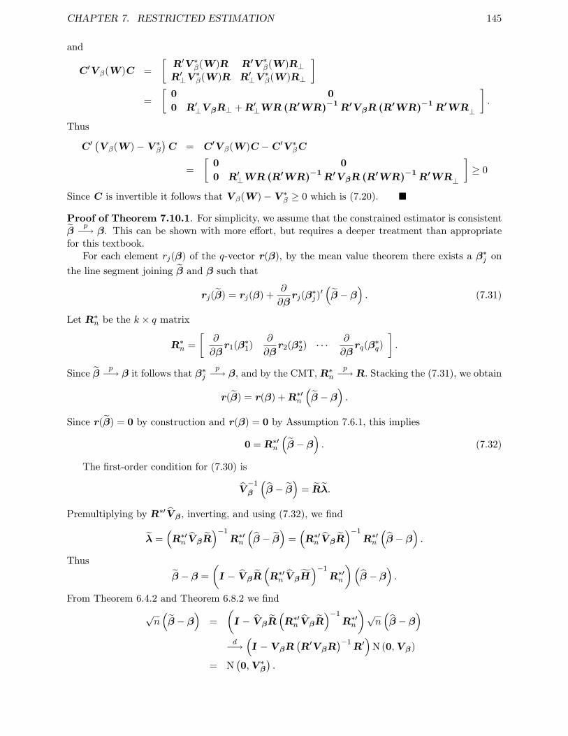
CHAPTER 7. RESTRICTED ESTIMATION 145
and
C ′V β(W )C =
[R′V ∗β(W )R R′V ∗β(W )R⊥R′⊥V
∗β(W )R R′⊥V
∗β(W )R⊥
]=
[0 0
0 R′⊥V βR⊥ +R′⊥WR (R′WR)−1R′V βR (R′WR)
−1R′WR⊥
].
Thus
C ′(V β(W )− V ∗β
)C = C ′V β(W )C −C ′V ∗βC
=
[0 0
0 R′⊥WR (R′WR)−1R′V βR (R′WR)
−1R′WR⊥
]≥ 0
Since C is invertible it follows that V β(W )− V ∗β ≥ 0 which is (7.20).
Proof of Theorem 7.10.1. For simplicity, we assume that the constrained estimator is consistentβ
p−→ β. This can be shown with more effort, but requires a deeper treatment than appropriatefor this textbook.
For each element rj(β) of the q-vector r(β), by the mean value theorem there exists a β∗j on
the line segment joining β and β such that
rj(β) = rj(β) +∂
∂βrj(β
∗j )′(β − β
). (7.31)
Let R∗n be the k × q matrix
R∗n =
[∂
∂βr1(β∗1)
∂
∂βr2(β∗2) · · · ∂
∂βrq(β
∗q)
].
Since βp−→ β it follows that β∗j
p−→ β, and by the CMT, R∗np−→ R. Stacking the (7.31), we obtain
r(β) = r(β) +R∗′n
(β − β
).
Since r(β) = 0 by construction and r(β) = 0 by Assumption 7.6.1, this implies
0 = R∗′n
(β − β
). (7.32)
The first-order condition for (7.30) is
V−1
β
(β − β
)= Rλ.
Premultiplying by R∗′V β, inverting, and using (7.32), we find
λ =(R∗′n V βR
)−1R∗′n
(β − β
)=(R∗′n V βR
)−1R∗′n
(β − β
).
Thus
β − β =
(I − V βR
(R∗′n V βH
)−1R∗′n
)(β − β
).
From Theorem 6.4.2 and Theorem 6.8.2 we find
√n(β − β
)=
(I − V βR
(R∗′n V βR
)−1R∗′n
)√n(β − β
)d−→(I − V βR
(R′V βR
)−1R′)
N (0,V β)
= N(0,V ∗β
).

CHAPTER 7. RESTRICTED ESTIMATION 146
Exercises
Exercise 7.1 In the model y = X1β1 +X2β2 + e, show directly from definition (7.3) that theCLS estimate of β = (β1,β2) subject to the constraint that β2 = 0 is the OLS regression of y onX1.
Exercise 7.2 In the model y = X1β1 +X2β2 + e, show directly from definition (7.3) that theCLS estimate of β = (β1,β2), subject to the constraint that β1 = c (where c is some given vector)is the OLS regression of y −X1c on X2.
Exercise 7.3 In the model y = X1β1 +X2β2 + e, with X1 and X2 each n × k, find the CLSestimate of β = (β1,β2), subject to the constraint that β1 = −β2.
Exercise 7.4 Verify that for β defined in (7.8) that R′β = c.
Exercise 7.5 Verify (7.14).
Exercise 7.6 Verify that the minimum distance estimator β with W n = Q−1
xx equals the CLSestimator.
Exercise 7.7 Prove Theorem 7.6.1.
Exercise 7.8 Prove Theorem 7.6.2.
Exercise 7.9 Prove Theorem 7.6.3. (Hint: Use that CLS is a special case of Theorem 7.6.2.)
Exercise 7.10 Verify that (7.18) is V β(W ) with W = V −1β .
Exercise 7.11 Prove (7.19). Hint: Use (7.18).
Exercise 7.12 Verify (7.21), (7.22) and (7.23)
Exercise 7.13 Verify (7.24), (7.25), and (7.26).
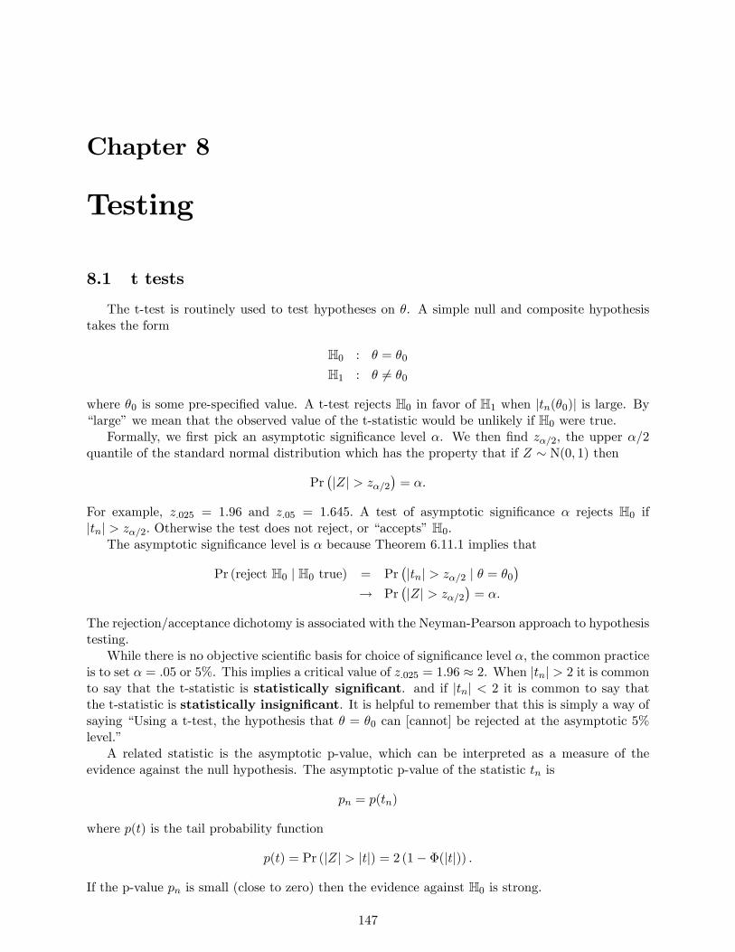
Chapter 8
Testing
8.1 t tests
The t-test is routinely used to test hypotheses on θ. A simple null and composite hypothesistakes the form
H0 : θ = θ0
H1 : θ 6= θ0
where θ0 is some pre-specified value. A t-test rejects H0 in favor of H1 when |tn(θ0)| is large. By“large”we mean that the observed value of the t-statistic would be unlikely if H0 were true.
Formally, we first pick an asymptotic significance level α. We then find zα/2, the upper α/2quantile of the standard normal distribution which has the property that if Z ∼ N(0, 1) then
Pr(|Z| > zα/2
)= α.
For example, z.025 = 1.96 and z.05 = 1.645. A test of asymptotic significance α rejects H0 if|tn| > zα/2. Otherwise the test does not reject, or “accepts”H0.
The asymptotic significance level is α because Theorem 6.11.1 implies that
Pr (reject H0 | H0 true) = Pr(|tn| > zα/2 | θ = θ0
)→ Pr
(|Z| > zα/2
)= α.
The rejection/acceptance dichotomy is associated with the Neyman-Pearson approach to hypothesistesting.
While there is no objective scientific basis for choice of significance level α, the common practiceis to set α = .05 or 5%. This implies a critical value of z.025 = 1.96 ≈ 2. When |tn| > 2 it is commonto say that the t-statistic is statistically significant. and if |tn| < 2 it is common to say thatthe t-statistic is statistically insignificant. It is helpful to remember that this is simply a way ofsaying “Using a t-test, the hypothesis that θ = θ0 can [cannot] be rejected at the asymptotic 5%level.”
A related statistic is the asymptotic p-value, which can be interpreted as a measure of theevidence against the null hypothesis. The asymptotic p-value of the statistic tn is
pn = p(tn)
where p(t) is the tail probability function
p(t) = Pr (|Z| > |t|) = 2 (1− Φ(|t|)) .
If the p-value pn is small (close to zero) then the evidence against H0 is strong.
147
CHAPTER 8. TESTING 148
An equivalent statement of a Neyman-Pearson test is to reject at the α% level if and only ifpn < α. Significance tests can be deduced directly from the p-value since for any α, pn < α ifand only if |tn| > zα/2. The p-value is more general, however, in that the reader is allowed to pickthe level of significance α, in contrast to Neyman-Pearson rejection/acceptance reporting wherethe researcher picks the significance level. (However, the Neyman-Pearson approach requires thereader to select the significance level before observing the p-value.)
Another helpful observation is that the p-value function is a unit-free transformation of the
t statistic. That is, under H0, pnd−→ U[0, 1], so the “unusualness” of the test statistic can be
compared to the easy-to-understand uniform distribution, regardless of the complication of thedistribution of the original test statistic. To see this fact, note that the asymptotic distribution of|tn| is F (x) = 1− p(x). Thus
Pr (1− pn ≤ u) = Pr (1− p(tn) ≤ u)
= Pr (F (tn) ≤ u)
= Pr(|tn| ≤ F−1(u)
)→ F
(F−1(u)
)= u,
establishing that 1− pnd−→ U[0, 1], from which it follows that pn
d−→ U[0, 1].
8.2 t-ratios
Some applied papers (especially older ones) report “t-ratios”for each estimated coeffi cient. Fora coeffi cient θ these are
tn = tn(0) =θ
s(θ),
the ratio of the coeffi cient estimate to its standard error, and equal the t-statistic for the test ofthe hypothesis H0 : θ = 0. Such papers often discuss the “significance” of certain variables orcoeffi cients, or describe “which regressors have a significant effect on y”by noting which t-ratiosexceed 2 in absolute value.
This is very poor econometric practice, and should be studiously avoided. It is a receipe forbanishment of your work to lower tier economics journals.
Fundamentally, the common t-ratio is a test for the hypothesis that a coeffi cient equals zero.This should be reported and discussed when this is an interesting economic hypothesis of interest.But if this is not the case, it is distracting.
Instead, when a coeffi cient θ is of interest, it is constructive to focus on the point estimate,its standard error, and its confidence interval. The point estimate gives our “best guess” for thevalue. The standard error is a measure of precision. The confidence interval gives us the rangeof values consistent with the data. If the standard error is large then the point estimate is not agood summary about θ. The endpoints of the confidence interval describe the bounds on the likelypossibilities. If the confidence interval embraces too broad a set of values for θ, then the datasetis not suffi ciently informative to render inferences about θ. On the other hand if the confidenceinterval is tight, then the data have produced an accurate estimate, and the focus should be onthe value and interpretation of this estimate. In contrast, the widely-seen statement “the t-ratio ishighly significant”has little interpretive value.
The above discussion requires that the researcher knows what the coeffi cient θ means (in termsof the economic problem) and can interpret values and magnitudes, not just signs. This is criticalfor good applied econometric practice.
CHAPTER 8. TESTING 149
8.3 Wald Tests
Sometimes θ = h(β) is a q × 1 vector, and it is desired to test the joint restrictions simultane-ously. We have the null and alternative
H0 : θ = θ0
H1 : θ 6= θ0.
A commonly used test ofH0 againstH1 is theWald statistic (6.34) evaluated at the null hypothesis
Wn = n(θ − θ0
)′V−1
θ
(θ − θ0
). (8.1)
Typically, we have θ = h(β) with asymptotic covariance matrix estimate
V θ = H′βV βHβ
where
Hβ =∂
∂βh(β).
ThenWn = n
(h(β)− θ0
)′ (H′βV βHβ
)−1 (h(β)− θ0
).
When h is a linear function of β, h(β) = R′β, then the Wald statistic simplifies to
Wn = n(R′β − θ0
)′ (R′V βR
)−1 (R′β − θ0
).
As shown in Theorem 6.14.2, when θ = θ0 then Wn −→ χ2q , a chi-square random variable with
q degrees of freedom.
Theorem 8.3.1 Under Assumption 1.5.1, Assumption 6.4.1,
rank(Hβ) = q, and H0, then Wnd−→ χ2
q.
An asymptotic Wald test rejects H0 in favor of H1 if Wn exceeds χ2q(α), the upper-α quantile
of the χ2q distribution. For example, χ
21(.05) = 3.84 = z2
.025. The Wald test fails to reject if Wn isless than χ2
q(α). As with t-tests, it is conventional to describe a Wald test as “significant” if Wn
exceeds the 5% critical value.Notice that the asymptotic distribution in Theorem 8.3.1 depends solely on q —the number of
restrictions being tested. It does not depend on k —the number of parameters estimated.The asymptotic p-value for Wn is pn = p(Wn), where p(x) = Pr
(χ2q ≥ x
)is the tail probability
function of the χ2q distribution. The Wald test rejects at the α% level if and only if pn < α, and
pn is asymptotically U[0, 1] under H0. In applied work it is good practice to report the p-value ofa Wald statistic, as it helps readers intrepret the magnitude of the statistic.
8.4 Minimum Distance Tests
The Wald test (8.1) measures the distance between the unrestricted estimate θ and the nullhypothesis θ0. A minimum distance test measures the distance between β and the restrictedestimate β of the previous chapter. Recall that under the restriction
h(β) = θ0
CHAPTER 8. TESTING 150
the effi cient minimum distance estimate solves the minimization problem
β = argminh(β)=θ0
Jn (β)
whereJn (β) = n
(β − β
)′V−1
β
(β − β
).
The minimum distance test statistic of H0 against H1 is
Jn = Jn(β) = minh(β)=θ0
Jn (β)
or more simply
Jn = n(β − β
)′V−1
β
(β − β
).
An asymptotic test rejects H0 in favor of H1 if Jn exceeds χ2q(α), the upper-α quantile of the χ2
q
distribution. Otherwise the test does not reject H0.When h(β) is linear it turns out that Jn = Wn, so the Wald and minimum distance tests are
equal. When h(β) is non-linear then the two tests are different.The chi-square critical value is justified by the following theorm.
Theorem 8.4.1 UnderAssumption 1.5.1, Assumption 6.4.1, rank(Hβ) =
q, and H0, then Jnd−→ χ2
q.
8.5 F Tests
Take the linear modely = X1β1 +X2β2 + e
where X1 is n× k1, X2 is n× k2, k = k1 + k2, and the null hypothesis is
H0 : β2 = 0.
In this case, θ = β2, and there are q = k2 restrictions. Also h(β) = R′β is linear with R =
(0I
)a selector matrix. We know that the Wald statistic takes the form
Wn = nθ′V−1
θ θ
= nβ′2
(R′V βR
)−1β2.
Now suppose that covariance matrix is computed under the assumption of homoskedasticity, so
that V β is replaced with V0
β = s2(n−1X ′X
)−1. We define the “homoskedastic”Wald statistic
W 0n = nθ
′ (V
0
θ
)−1θ
= nβ′2
(R′V 0
βR)−1
β2.
What we show in this section is that this Wald statistic can be written very simply using theformula
W 0n = (n− k)
(e′e− e′ee′e
)(8.2)
CHAPTER 8. TESTING 151
wheree = y −X1β1, β1 =
(X ′1X1
)−1X ′1y
are from OLS of y on X1, and
e = y −Xβ, β =(X ′X
)−1X ′y
are from OLS of y on X = (X1,X2).The elegant feature about (8.2) is that it is directly computable from the standard output
from two simple OLS regressions, as the sum of squared errors is a typical output from statisticalpackages. This statistic is typically reported as an “F-statistic”which is defined as
Fn =W 0n
k2=
(e′e− e′e
)/k2
e′e/(n− k).
While it should be emphasized that equality (8.2) only holds if V 0β = s2
(n−1X ′X
)−1, still this
formula often finds good use in reading applied papers. Because of this connection we call (8.2) theF form of the Wald statistic. (We can also call W 0
n a homoskedastic form of the Wald statistic.)We now derive expression (8.2). First, note that by partitioned matrix inversion (A.4)
R′(X ′X
)−1R = R′
(X ′1X1 X ′1X2
X ′2X1 X ′2X2
)−1
R =(X ′2M1X2
)−1
whereM1 = I −X1(X ′1X1)−1X ′1. Thus(R′V 0
βR)−1
= s−2n−1(R′(X ′X
)−1R)−1
= s−2n−1(X ′2M1X2
)and
W 0n = nβ
′2
(R′V 0
βR)−1
β2
=β′2 (X ′2M1X2) β2
s2.
To simplify this expression further, note that if we regress y on X1 alone, the residual ise = M1y. Now consider the residual regression of e on X2 = M1X2. By the FWL theorem,e = X2β2 + e and X
′2e = 0. Thus
e′e =(X2β2 + e
)′ (X2β2 + e
)= β
′2X′2X2β2 + e′e
= β′2X′2M1X2β2 + e′e,
or alternatively,β′2X′2M1X2β2 = e′e− e′e.
Also, sinces2 = (n− k)−1 e′e
we conclude that
W 0n = (n− k)
(e′e− e′ee′e
)as claimed.
In many statistical packages, when an OLS regression is estimated, an “F-statistic”is reported.This is Fn when X1 is a vector of ones, so H0 is an intercept-only model. This special F statistic is
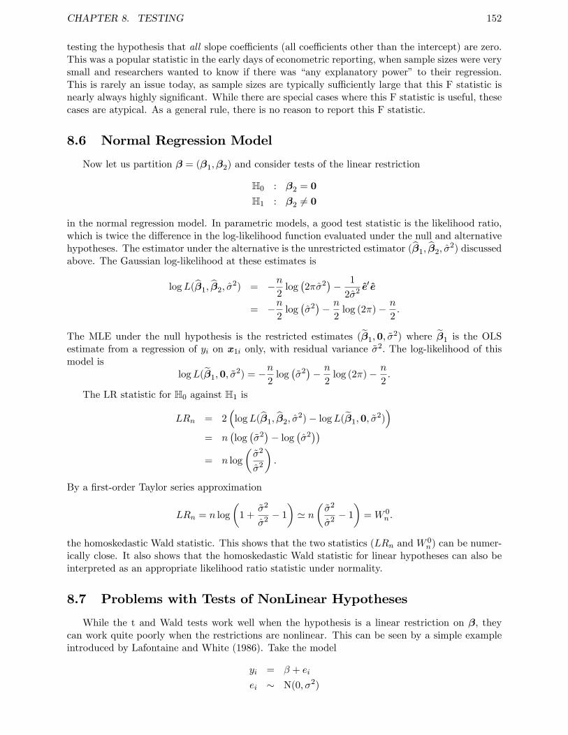
CHAPTER 8. TESTING 152
testing the hypothesis that all slope coeffi cients (all coeffi cients other than the intercept) are zero.This was a popular statistic in the early days of econometric reporting, when sample sizes were verysmall and researchers wanted to know if there was “any explanatory power” to their regression.This is rarely an issue today, as sample sizes are typically suffi ciently large that this F statistic isnearly always highly significant. While there are special cases where this F statistic is useful, thesecases are atypical. As a general rule, there is no reason to report this F statistic.
8.6 Normal Regression Model
Now let us partition β = (β1,β2) and consider tests of the linear restriction
H0 : β2 = 0
H1 : β2 6= 0
in the normal regression model. In parametric models, a good test statistic is the likelihood ratio,which is twice the difference in the log-likelihood function evaluated under the null and alternativehypotheses. The estimator under the alternative is the unrestricted estimator (β1, β2, σ
2) discussedabove. The Gaussian log-likelihood at these estimates is
logL(β1, β2, σ2) = −n
2log(2πσ2
)− 1
2σ2 e′e
= −n2
log(σ2)− n
2log (2π)− n
2.
The MLE under the null hypothesis is the restricted estimates (β1,0, σ2) where β1 is the OLS
estimate from a regression of yi on x1i only, with residual variance σ2. The log-likelihood of thismodel is
logL(β1,0, σ2) = −n
2log(σ2)− n
2log (2π)− n
2.
The LR statistic for H0 against H1 is
LRn = 2(
logL(β1, β2, σ2)− logL(β1,0, σ
2))
= n(log(σ2)− log
(σ2))
= n log
(σ2
σ2
).
By a first-order Taylor series approximation
LRn = n log
(1 +
σ2
σ2 − 1
)' n
(σ2
σ2 − 1
)= W 0
n .
the homoskedastic Wald statistic. This shows that the two statistics (LRn and W 0n) can be numer-
ically close. It also shows that the homoskedastic Wald statistic for linear hypotheses can also beinterpreted as an appropriate likelihood ratio statistic under normality.
8.7 Problems with Tests of NonLinear Hypotheses
While the t and Wald tests work well when the hypothesis is a linear restriction on β, theycan work quite poorly when the restrictions are nonlinear. This can be seen by a simple exampleintroduced by Lafontaine and White (1986). Take the model
yi = β + ei
ei ∼ N(0, σ2)
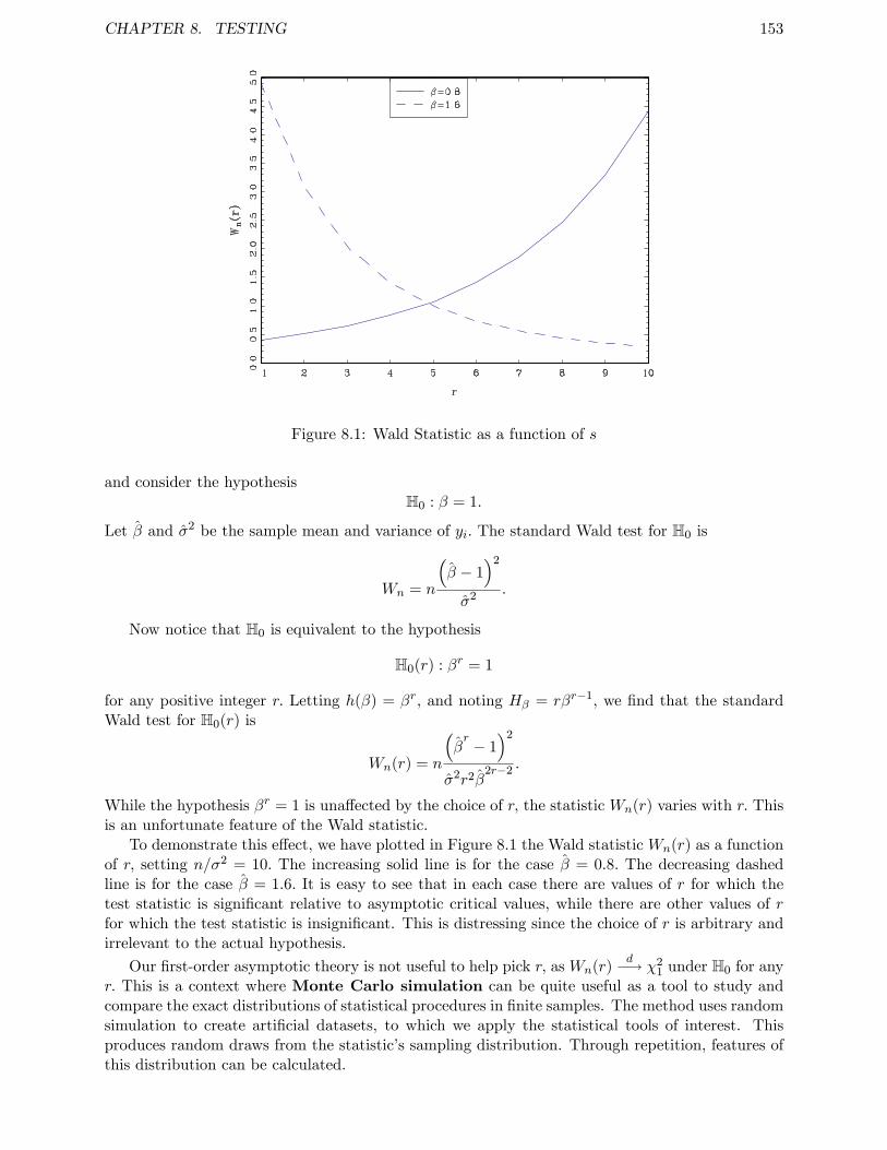
CHAPTER 8. TESTING 153
Figure 8.1: Wald Statistic as a function of s
and consider the hypothesisH0 : β = 1.
Let β and σ2 be the sample mean and variance of yi. The standard Wald test for H0 is
Wn = n
(β − 1
)2
σ2 .
Now notice that H0 is equivalent to the hypothesis
H0(r) : βr = 1
for any positive integer r. Letting h(β) = βr, and noting Hβ = rβr−1, we find that the standardWald test for H0(r) is
Wn(r) = n
(βr − 1
)2
σ2r2β2r−2 .
While the hypothesis βr = 1 is unaffected by the choice of r, the statistic Wn(r) varies with r. Thisis an unfortunate feature of the Wald statistic.
To demonstrate this effect, we have plotted in Figure 8.1 the Wald statistic Wn(r) as a functionof r, setting n/σ2 = 10. The increasing solid line is for the case β = 0.8. The decreasing dashedline is for the case β = 1.6. It is easy to see that in each case there are values of r for which thetest statistic is significant relative to asymptotic critical values, while there are other values of rfor which the test statistic is insignificant. This is distressing since the choice of r is arbitrary andirrelevant to the actual hypothesis.
Our first-order asymptotic theory is not useful to help pick r, asWn(r)d−→ χ2
1 under H0 for anyr. This is a context where Monte Carlo simulation can be quite useful as a tool to study andcompare the exact distributions of statistical procedures in finite samples. The method uses randomsimulation to create artificial datasets, to which we apply the statistical tools of interest. Thisproduces random draws from the statistic’s sampling distribution. Through repetition, features ofthis distribution can be calculated.
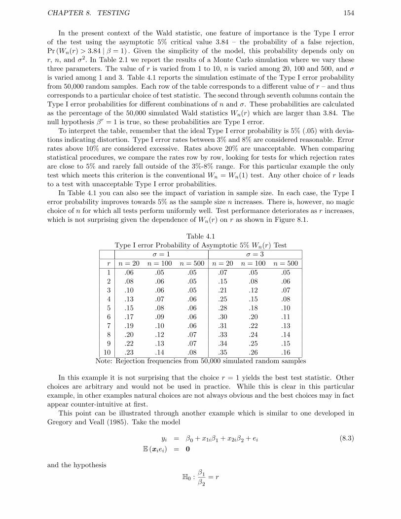
CHAPTER 8. TESTING 154
In the present context of the Wald statistic, one feature of importance is the Type I errorof the test using the asymptotic 5% critical value 3.84 — the probability of a false rejection,Pr (Wn(r) > 3.84 | β = 1) . Given the simplicity of the model, this probability depends only onr, n, and σ2. In Table 2.1 we report the results of a Monte Carlo simulation where we vary thesethree parameters. The value of r is varied from 1 to 10, n is varied among 20, 100 and 500, and σis varied among 1 and 3. Table 4.1 reports the simulation estimate of the Type I error probabilityfrom 50,000 random samples. Each row of the table corresponds to a different value of r —and thuscorresponds to a particular choice of test statistic. The second through seventh columns contain theType I error probabilities for different combinations of n and σ. These probabilities are calculatedas the percentage of the 50,000 simulated Wald statistics Wn(r) which are larger than 3.84. Thenull hypothesis βr = 1 is true, so these probabilities are Type I error.
To interpret the table, remember that the ideal Type I error probability is 5% (.05) with devia-tions indicating distortion. Type I error rates between 3% and 8% are considered reasonable. Errorrates above 10% are considered excessive. Rates above 20% are unacceptable. When comparingstatistical procedures, we compare the rates row by row, looking for tests for which rejection ratesare close to 5% and rarely fall outside of the 3%-8% range. For this particular example the onlytest which meets this criterion is the conventional Wn = Wn(1) test. Any other choice of r leadsto a test with unacceptable Type I error probabilities.
In Table 4.1 you can also see the impact of variation in sample size. In each case, the Type Ierror probability improves towards 5% as the sample size n increases. There is, however, no magicchoice of n for which all tests perform uniformly well. Test performance deteriorates as r increases,which is not surprising given the dependence of Wn(r) on r as shown in Figure 8.1.
Table 4.1Type I error Probability of Asymptotic 5% Wn(r) Test
σ = 1 σ = 3
r n = 20 n = 100 n = 500 n = 20 n = 100 n = 500
1 .06 .05 .05 .07 .05 .052 .08 .06 .05 .15 .08 .063 .10 .06 .05 .21 .12 .074 .13 .07 .06 .25 .15 .085 .15 .08 .06 .28 .18 .106 .17 .09 .06 .30 .20 .117 .19 .10 .06 .31 .22 .138 .20 .12 .07 .33 .24 .149 .22 .13 .07 .34 .25 .1510 .23 .14 .08 .35 .26 .16
Note: Rejection frequencies from 50,000 simulated random samples
In this example it is not surprising that the choice r = 1 yields the best test statistic. Otherchoices are arbitrary and would not be used in practice. While this is clear in this particularexample, in other examples natural choices are not always obvious and the best choices may in factappear counter-intuitive at first.
This point can be illustrated through another example which is similar to one developed inGregory and Veall (1985). Take the model
yi = β0 + x1iβ1 + x2iβ2 + ei (8.3)
E (xiei) = 0
and the hypothesis
H0 :β1
β2
= r
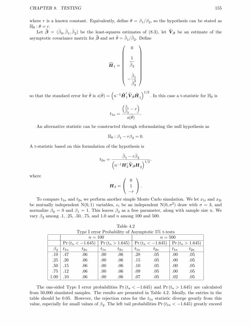
CHAPTER 8. TESTING 155
where r is a known constant. Equivalently, define θ = β1/β2, so the hypothesis can be stated asH0 : θ = r.
Let β = (β0, β1, β2) be the least-squares estimates of (8.3), let V β be an estimate of theasymptotic covariance matrix for β and set θ = β1/β2. Define
H1 =
0
1
β2
− β1
β2
2
so that the standard error for θ is s(θ) =
(n−1H
′1V βH1
)1/2. In this case a t-statistic for H0 is
t1n =
(β1β2− r)
s(θ).
An alternative statistic can be constructed through reformulating the null hypothesis as
H0 : β1 − rβ2 = 0.
A t-statistic based on this formulation of the hypothesis is
t2n =β1 − rβ2(
n−1H ′2V βH2
)1/2.
where
H2 =
01−r
.
To compare t1n and t2n we perform another simple Monte Carlo simulation. We let x1i and x2i
be mutually independent N(0, 1) variables, ei be an independent N(0, σ2) draw with σ = 3, andnormalize β0 = 0 and β1 = 1. This leaves β2 as a free parameter, along with sample size n. Wevary β2 among .1, .25, .50, .75, and 1.0 and n among 100 and 500.
Table 4.2Type I error Probability of Asymptotic 5% t-tests
n = 100 n = 500
Pr (tn < −1.645) Pr (tn > 1.645) Pr (tn < −1.645) Pr (tn > 1.645)
β2 t1n t2n t1n t2n t1n t2n t1n t2n.10 .47 .06 .00 .06 .28 .05 .00 .05.25 .26 .06 .00 .06 .15 .05 .00 .05.50 .15 .06 .00 .06 .10 .05 .00 .05.75 .12 .06 .00 .06 .09 .05 .00 .051.00 .10 .06 .00 .06 .07 .05 .02 .05
The one-sided Type I error probabilities Pr (tn < −1.645) and Pr (tn > 1.645) are calculatedfrom 50,000 simulated samples. The results are presented in Table 4.2. Ideally, the entries in thetable should be 0.05. However, the rejection rates for the t1n statistic diverge greatly from thisvalue, especially for small values of β2. The left tail probabilities Pr (t1n < −1.645) greatly exceed
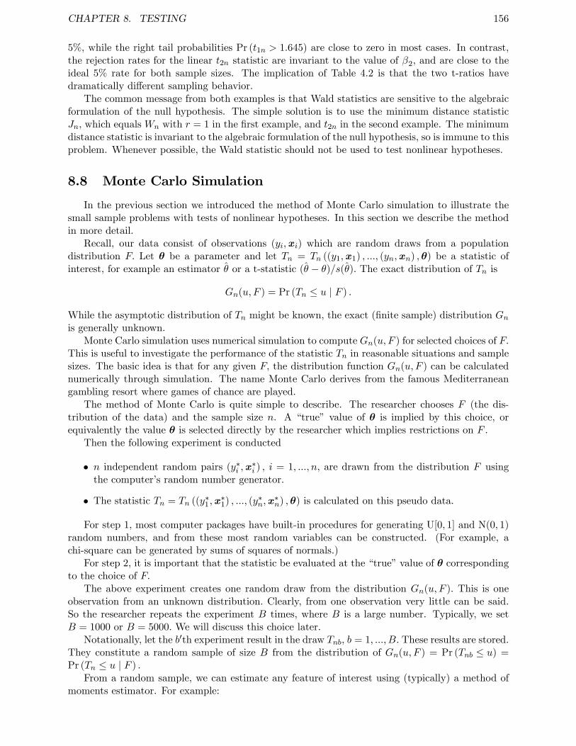
CHAPTER 8. TESTING 156
5%, while the right tail probabilities Pr (t1n > 1.645) are close to zero in most cases. In contrast,the rejection rates for the linear t2n statistic are invariant to the value of β2, and are close to theideal 5% rate for both sample sizes. The implication of Table 4.2 is that the two t-ratios havedramatically different sampling behavior.
The common message from both examples is that Wald statistics are sensitive to the algebraicformulation of the null hypothesis. The simple solution is to use the minimum distance statisticJn, which equals Wn with r = 1 in the first example, and t2n in the second example. The minimumdistance statistic is invariant to the algebraic formulation of the null hypothesis, so is immune to thisproblem. Whenever possible, the Wald statistic should not be used to test nonlinear hypotheses.
8.8 Monte Carlo Simulation
In the previous section we introduced the method of Monte Carlo simulation to illustrate thesmall sample problems with tests of nonlinear hypotheses. In this section we describe the methodin more detail.
Recall, our data consist of observations (yi,xi) which are random draws from a populationdistribution F. Let θ be a parameter and let Tn = Tn ((y1,x1) , ..., (yn,xn) ,θ) be a statistic ofinterest, for example an estimator θ or a t-statistic (θ − θ)/s(θ). The exact distribution of Tn is
Gn(u, F ) = Pr (Tn ≤ u | F ) .
While the asymptotic distribution of Tn might be known, the exact (finite sample) distribution Gnis generally unknown.
Monte Carlo simulation uses numerical simulation to compute Gn(u, F ) for selected choices of F.This is useful to investigate the performance of the statistic Tn in reasonable situations and samplesizes. The basic idea is that for any given F, the distribution function Gn(u, F ) can be calculatednumerically through simulation. The name Monte Carlo derives from the famous Mediterraneangambling resort where games of chance are played.
The method of Monte Carlo is quite simple to describe. The researcher chooses F (the dis-tribution of the data) and the sample size n. A “true” value of θ is implied by this choice, orequivalently the value θ is selected directly by the researcher which implies restrictions on F .
Then the following experiment is conducted
• n independent random pairs (y∗i ,x∗i ) , i = 1, ..., n, are drawn from the distribution F using
the computer’s random number generator.
• The statistic Tn = Tn ((y∗1,x∗1) , ..., (y∗n,x
∗n) ,θ) is calculated on this pseudo data.
For step 1, most computer packages have built-in procedures for generating U[0, 1] and N(0, 1)random numbers, and from these most random variables can be constructed. (For example, achi-square can be generated by sums of squares of normals.)
For step 2, it is important that the statistic be evaluated at the “true”value of θ correspondingto the choice of F.
The above experiment creates one random draw from the distribution Gn(u, F ). This is oneobservation from an unknown distribution. Clearly, from one observation very little can be said.So the researcher repeats the experiment B times, where B is a large number. Typically, we setB = 1000 or B = 5000. We will discuss this choice later.
Notationally, let the b′th experiment result in the draw Tnb, b = 1, ..., B. These results are stored.They constitute a random sample of size B from the distribution of Gn(u, F ) = Pr (Tnb ≤ u) =Pr (Tn ≤ u | F ) .
From a random sample, we can estimate any feature of interest using (typically) a method ofmoments estimator. For example:
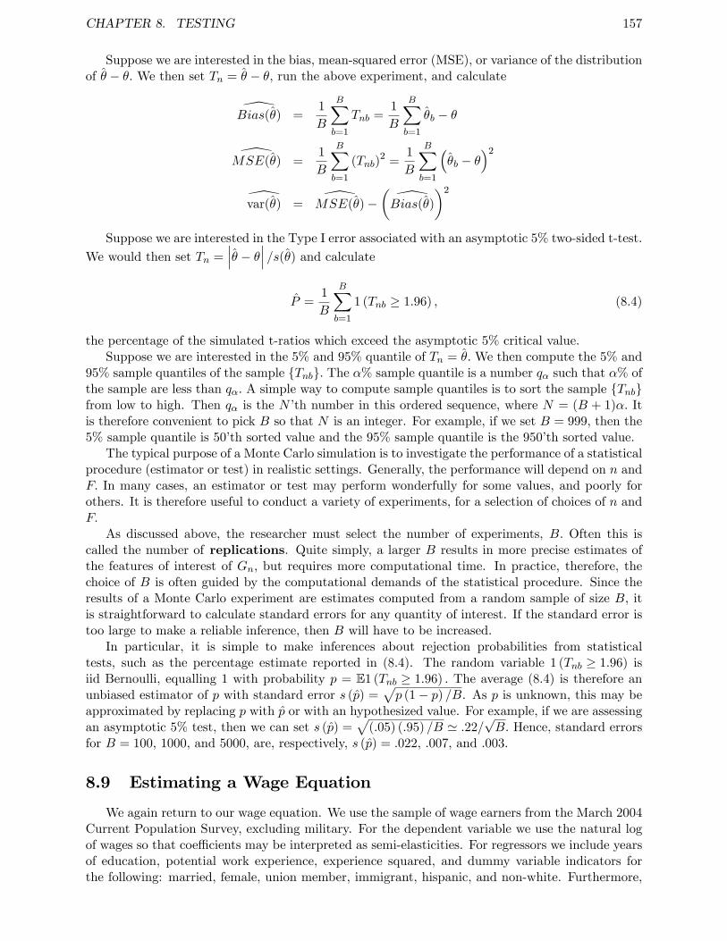
CHAPTER 8. TESTING 157
Suppose we are interested in the bias, mean-squared error (MSE), or variance of the distributionof θ − θ. We then set Tn = θ − θ, run the above experiment, and calculate
Bias(θ) =1
B
B∑b=1
Tnb =1
B
B∑b=1
θb − θ
MSE(θ) =1
B
B∑b=1
(Tnb)2 =
1
B
B∑b=1
(θb − θ
)2
var(θ) = MSE(θ)−(Bias(θ)
)2
Suppose we are interested in the Type I error associated with an asymptotic 5% two-sided t-test.
We would then set Tn =∣∣∣θ − θ∣∣∣ /s(θ) and calculate
P =1
B
B∑b=1
1 (Tnb ≥ 1.96) , (8.4)
the percentage of the simulated t-ratios which exceed the asymptotic 5% critical value.Suppose we are interested in the 5% and 95% quantile of Tn = θ.We then compute the 5% and
95% sample quantiles of the sample Tnb. The α% sample quantile is a number qα such that α% ofthe sample are less than qα. A simple way to compute sample quantiles is to sort the sample Tnbfrom low to high. Then qα is the N’th number in this ordered sequence, where N = (B + 1)α. Itis therefore convenient to pick B so that N is an integer. For example, if we set B = 999, then the5% sample quantile is 50’th sorted value and the 95% sample quantile is the 950’th sorted value.
The typical purpose of a Monte Carlo simulation is to investigate the performance of a statisticalprocedure (estimator or test) in realistic settings. Generally, the performance will depend on n andF. In many cases, an estimator or test may perform wonderfully for some values, and poorly forothers. It is therefore useful to conduct a variety of experiments, for a selection of choices of n andF.
As discussed above, the researcher must select the number of experiments, B. Often this iscalled the number of replications. Quite simply, a larger B results in more precise estimates ofthe features of interest of Gn, but requires more computational time. In practice, therefore, thechoice of B is often guided by the computational demands of the statistical procedure. Since theresults of a Monte Carlo experiment are estimates computed from a random sample of size B, itis straightforward to calculate standard errors for any quantity of interest. If the standard error istoo large to make a reliable inference, then B will have to be increased.
In particular, it is simple to make inferences about rejection probabilities from statisticaltests, such as the percentage estimate reported in (8.4). The random variable 1 (Tnb ≥ 1.96) isiid Bernoulli, equalling 1 with probability p = E1 (Tnb ≥ 1.96) . The average (8.4) is therefore anunbiased estimator of p with standard error s (p) =
√p (1− p) /B. As p is unknown, this may be
approximated by replacing p with p or with an hypothesized value. For example, if we are assessingan asymptotic 5% test, then we can set s (p) =
√(.05) (.95) /B ' .22/
√B. Hence, standard errors
for B = 100, 1000, and 5000, are, respectively, s (p) = .022, .007, and .003.
8.9 Estimating a Wage Equation
We again return to our wage equation. We use the sample of wage earners from the March 2004Current Population Survey, excluding military. For the dependent variable we use the natural logof wages so that coeffi cients may be interpreted as semi-elasticities. For regressors we include yearsof education, potential work experience, experience squared, and dummy variable indicators forthe following: married, female, union member, immigrant, hispanic, and non-white. Furthermore,
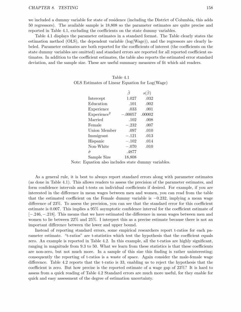
CHAPTER 8. TESTING 158
we included a dummy variable for state of residence (including the District of Columbia, this adds50 regressors). The available sample is 18,808 so the parameter estimates are quite precise andreported in Table 4.1, excluding the coeffi cients on the state dummy variables.
Table 4.1 displays the parameter estimates in a standard format. The Table clearly states theestimation method (OLS), the dependent variable (log(Wage)), and the regressors are clearly la-beled. Parameter estimates are both reported for the coeffi cients of interest (the coeffi cients on thestate dummy variables are omitted) and standard errors are reported for all reported coeffi cient es-timates. In addition to the coeffi cient estimates, the table also reports the estimated error standarddeviation, and the sample size. These are useful summary measures of fit which aid readers.
Table 4.1OLS Estimates of Linear Equation for Log(Wage)
β s(β)Intercept 1.027 .032Education .101 .002Experience .033 .001Experience2 −.00057 .00002Married .102 .008Female −.232 .007Union Member .097 .010Immigrant −.121 .013Hispanic −.102 .014Non-White −.070 .010σ .4877Sample Size 18,808
Note: Equation also includes state dummy variables.
As a general rule, it is best to always report standard errors along with parameter estimates(as done in Table 4.1). This allows readers to assess the precision of the parameter estimates, andform confidence intervals and t-tests on individual coeffi cients if desired. For example, if you areinterested in the difference in mean wages between men and women, you can read from the tablethat the estimated coeffi cient on the Female dummy variable is −0.232, implying a mean wagedifference of 23%. To assess the precision, you can see that the standard error for this coeffi cientestimate is 0.007. This implies a 95% asymptotic confidence interval for the coeffi cient estimate of[−.246,−.218]. This means that we have estimated the difference in mean wages between men andwomen to lie between 22% and 25%. I interpret this as a precise estimate because there is not animportant difference between the lower and upper bound.
Instead of reporting standard errors, some empirical researchers report t-ratios for each pa-rameter estimate. “t-ratios” are t-statistics which test the hypothesis that the coeffi cient equalszero. An example is reported in Table 4.2. In this example, all the t-ratios are highly significant,ranging in magnitude from 9.3 to 50. What we learn from these statistics is that these coeffi cientsare non-zero, but not much more. In a sample of this size this finding is rather uninteresting;consequently the reporting of t-ratios is a waste of space. Again consider the male-female wagedifference. Table 4.2 reports that the t-ratio is 33, enabling us to reject the hypothesis that thecoeffi cient is zero. But how precise is the reported estimate of a wage gap of 23%? It is hard toassess from a quick reading of Table 4.2 Standard errors are much more useful, for they enable forquick and easy assessment of the degree of estimation uncertainty.
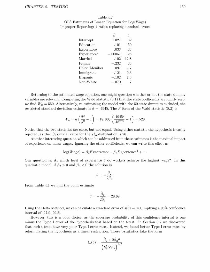
CHAPTER 8. TESTING 159
Table 4.2OLS Estimates of Linear Equation for Log(Wage)
Improper Reporting: t-ratios replacing standard errors
β tIntercept 1.027 32Education .101 50Experience .033 33Experience2 −.00057 28Married .102 12.8Female −.232 33Union Member .097 9.7Immigrant −.121 9.3Hispanic −.102 7.3Non-White −.070 7
Returning to the estimated wage equation, one might question whether or not the state dummyvariables are relevant. Computing the Wald statistic (8.1) that the state coeffi cients are jointly zero,we find Wn = 550. Alternatively, re-estimating the model with the 50 state dummies excluded, therestricted standard deviation estimate is σ = .4945. The F form of the Wald statistic (8.2) is
Wn = n
(σ2
σ2 − 1
)= 18, 808
(.49452
.48772− 1
)= 528.
Notice that the two statistics are close, but not equal. Using either statistic the hypothesis is easilyrejected, as the 1% critical value for the χ2
50 distribution is 76.Another interesting question which can be addressed from these estimates is the maximal impact
of experience on mean wages. Ignoring the other coeffi cients, we can write this effect as
log(Wage) = β2Experience+ β3Experience2 + · · ·
Our question is: At which level of experience θ do workers achieve the highest wage? In thisquadratic model, if β2 > 0 and β3 < 0 the solution is
θ = − β2
2β3
.
From Table 4.1 we find the point estimate
θ = − β2
2β3
= 28.69.
Using the Delta Method, we can calculate a standard error of s(θ) = .40, implying a 95% confidenceinterval of [27.9, 29.5].
However, this is a poor choice, as the coverage probability of this confidence interval is oneminus the Type I error of the hypothesis test based on the t-test. In Section 8.7 we discoveredthat such t-tests have very poor Type I error rates. Instead, we found better Type I error rates byreformulating the hypothesis as a linear restriction. These t-statistics take the form
tn(θ) =β2 + 2β3θ(h′θV hθ
)1/2

CHAPTER 8. TESTING 160
where
hθ =
(12θ
)and V is the covariance matrix for (β2 β3).
In the present context we are interested in forming a confidence interval, not testing a hypothesis,so we have to go one step further. Our desired confidence interval will be the set of parameter valuesθ which are not rejected by the hypothesis test. This is the set of θ such that |tn(θ)| ≤ 1.96. Sincetn(θ) is a non-linear function of θ, there is not a simple expression for this set, but it can be foundnumerically quite easily. This set is [27.0, 29.5]. Notice that the upper end of the confidence intervalis the same as that from the delta method, but the lower end is substantially lower.
CHAPTER 8. TESTING 161
Exercises
Exercise 8.1 Prove that if an additional regressor Xk+1 is added to X, Theil’s adjusted R2
increases if and only if |tk+1| > 1, where tk+1 = βk+1/s(βk+1) is the t-ratio for βk+1 and
s(βk+1) =(s2[(X ′X)−1]k+1,k+1
)1/2is the homoskedasticity-formula standard error.
Exercise 8.2 You have two independent samples (y1,X1) and (y2,X2) which satisfy y1 = X1β1+e1 and y2 = X2β2 + e2, where E (x1ie1i) = 0 and E (x2ie2i) = 0, and both X1 and X2 have kcolumns. Let β1 and β2 be the OLS estimates of β1 and β2. For simplicity, you may assume thatboth samples have the same number of observations n.
(a) Find the asymptotic distribution of√n((β2 − β1
)− (β2 − β1)
)as n→∞.
(b) Find an appropriate test statistic for H0 : β2 = β1.
(c) Find the asymptotic distribution of this statistic under H0.
Exercise 8.3 The data set invest.dat contains data on 565 U.S. firms extracted from Compustatfor the year 1987. The variables, in order, are
• Ii Investment to Capital Ratio (multiplied by 100).
• Qi Total Market Value to Asset Ratio (Tobin’s Q).
• Ci Cash Flow to Asset Ratio.
• Di Long Term Debt to Asset Ratio.
The flow variables are annual sums for 1987. The stock variables are beginning of year.
(a) Estimate a linear regression of Ii on the other variables. Calculate appropriate standarderrors.
(b) Calculate asymptotic confidence intervals for the coeffi cients.
(c) This regression is related to Tobin’s q theory of investment, which suggests that investmentshould be predicted solely by Qi. Thus the coeffi cient on Qi should be positive and the othersshould be zero. Test the joint hypothesis that the coeffi cients on Ci and Di are zero. Test thehypothesis that the coeffi cient on Qi is zero. Are the results consistent with the predictionsof the theory?
(d) Now try a non-linear (quadratic) specification. Regress Ii on Qi, Ci, Di, Q2i , C
2i , D
2i , QiCi,
QiDi, CiDi. Test the joint hypothesis that the six interaction and quadratic coeffi cients arezero.
Exercise 8.4 In a paper in 1963, Marc Nerlove analyzed a cost function for 145 American electriccompanies. (The problem is discussed in Example 8.3 of Greene, section 1.7 of Hayashi, and theempirical exercise in Chapter 1 of Hayashi). The data file nerlov.dat contains his data. Thevariables are described on page 77 of Hayashi. Nerlov was interested in estimating a cost function:TC = f(Q,PL, PF, PK).
CHAPTER 8. TESTING 162
(a) First estimate an unrestricted Cobb-Douglass specification
log TCi = β1 + β2 logQi + β3 logPLi + β4 logPKi + β5 logPFi + ei. (8.5)
Report parameter estimates and standard errors. You should obtain the same OLS estimatesas in Hayashi’s equation (1.7.7), but your standard errors may differ.
(b) What is the economic meaning of the restriction H0 : β3 + β4 + β5 = 1?
(c) Estimate (8.5) by constrained least-squares imposing β3+β4+β5 = 1. Report your parameterestimates and standard errors.
(d) Estimate (8.5) by effi cient minimum distance imposing β3 + β4 + β5 = 1. Report yourparameter estimates and standard errors.
(e) Test H0 : β3 + β4 + β5 = 1 using a Wald statistic
(f) Test H0 : β3 + β4 + β5 = 1 using a minimum distance statistic.
Chapter 9
Additional Regression Topics
9.1 Generalized Least Squares
In the projection model, we know that the least-squares estimator is semi-parametrically effi cientfor the projection coeffi cient. However, in the linear regression model
yi = x′iβ + ei
E (ei | xi) = 0,
the least-squares estimator is ineffi cient. The theory of Chamberlain (1987) can be used to showthat in this model the semiparametric effi ciency bound is obtained by the Generalized LeastSquares (GLS) estimator (5.12) introduced in Section 5.4.1. The GLS estimator is sometimescalled the Aitken estimator. The GLS estimator (9.1) is infeasible since the matrix D is unknown.A feasible GLS (FGLS) estimator replaces the unknown D with an estimate D = diagσ2
1, ..., σ2n.
We now discuss this estimation problem.Suppose that we model the conditional variance using the parametric form
σ2i = α0 + z′1iα1
= α′zi,
where z1i is some q × 1 function of xi. Typically, z1i are squares (and perhaps levels) of some (orall) elements of xi. Often the functional form is kept simple for parsimony.
Let ηi = e2i . Then
E (ηi | xi) = α0 + z′1iα1
and we have the regression equation
ηi = α0 + z′1iα1 + ξi (9.1)
E (ξi | xi) = 0.
This regression error ξi is generally heteroskedastic and has the conditional variance
var (ξi | xi) = var(e2i | xi
)= E
((e2i − E
(e2i | xi
))2 | xi)= E
(e4i | xi
)−(E(e2i | xi
))2.
Suppose ei (and thus ηi) were observed. Then we could estimate α by OLS:
α =(Z ′Z
)−1Z ′η
p−→ α
163
CHAPTER 9. ADDITIONAL REGRESSION TOPICS 164
and √n (α−α)
d−→ N (0,V α)
whereV α =
(E(ziz′i
))−1 E(ziz′iξ
2i
) (E(ziz′i
))−1. (9.2)
While ei is not observed, we have the OLS residual ei = yi − x′iβ = ei − x′i(β − β). Thus
φi ≡ η − ηi= e2
i − e2i
= −2eix′i
(β − β
)+ (β − β)′xix
′i(β − β).
And then
1√n
n∑i=1
ziφi =−2
n
n∑i=1
zieix′i
√n(β − β
)+
1
n
n∑i=1
zi(β − β)′xix′i(β − β)
√n
p−→ 0
Letα =
(Z ′Z
)−1Z ′η (9.3)
be from OLS regression of ηi on zi. Then√n (α−α) =
√n (α−α) +
(n−1Z ′Z
)−1n−1/2Z ′φ
d−→ N (0,V α) (9.4)
Thus the fact that ηi is replaced with ηi is asymptotically irrelevant. We call (9.3) the skedasticregression, as it is estimating the conditional variance of the regression of yi on xi. We have shownthat α is consistently estimated by a simple procedure, and hence we can estimate σ2
i = z′iα by
σ2i = α′zi. (9.5)
Suppose that σ2i > 0 for all i. Then set
D = diagσ21, ..., σ
2n
and
β =(X ′D
−1X)−1
X ′D−1y.
This is the feasible GLS, or FGLS, estimator of β. Since there is not a unique specification forthe conditional variance the FGLS estimator is not unique, and will depend on the model (andestimation method) for the skedastic regression.
One typical problem with implementation of FGLS estimation is that in the linear specification(9.1), there is no guarantee that σ2
i > 0 for all i. If σ2i < 0 for some i, then the FGLS estimator
is not well defined. Furthermore, if σ2i ≈ 0 for some i then the FGLS estimator will force the
regression equation through the point (yi,xi), which is undesirable. This suggests that there is aneed to bound the estimated variances away from zero. A trimming rule takes the form
σ2i = max[σ2
i , cσ2]
for some c > 0. For example, setting c = 1/4 means that the conditional variance function isconstrained to exceed one-fourth of the unconditional variance. As there is no clear method toselect c, this introduces a degree of arbitrariness. In this context it is useful to re-estimate themodel with several choices for the trimming parameter. If the estimates turn out to be sensitive toits choice, the estimation method should probably be reconsidered.
It is possible to show that if the skedastic regression is correctly specified, then FGLS is asymp-totically equivalent to GLS. As the proof is tricky, we just state the result without proof.
CHAPTER 9. ADDITIONAL REGRESSION TOPICS 165
Theorem 9.1.1 If the skedastic regression is correctly specified,
√n(βGLS − βFGLS
)p−→ 0,
and thus √n(βFGLS − β
)d−→ N (0,V β) ,
whereV β =
(E(σ−2i xix
′i
))−1.
Examining the asymptotic distribution of Theorem 9.1.1, the natural estimator of the asymp-totic variance of β is
V0
β =
(1
n
n∑i=1
σ−2i xix
′i
)−1
=
(1
nX ′D
−1X
)−1
.
which is consistent for V β as n → ∞. This estimator V 0
β is appropriate when the skedasticregression (9.1) is correctly specified.
It may be the case that α′zi is only an approximation to the true conditional variance σ2i =
E(e2i | xi). In this case we interpret α′zi as a linear projection of e2
i on zi. β should perhaps becalled a quasi-FGLS estimator of β. Its asymptotic variance is not that given in Theorem 9.1.1.Instead,
V β =(E((α′zi
)−1xix
′i
))−1 (E((α′zi
)−2σ2ixix
′i
))(E((α′zi
)−1xix
′i
))−1.
V β takes a sandwich form similar to the covariance matrix of the OLS estimator. Unless σ2i = α′zi,
V0
β is inconsistent for V β.
An appropriate solution is to use a White-type estimator in place of V0
β. This may be writtenas
V β =
(1
n
n∑i=1
σ−2i xix
′i
)−1(1
n
n∑i=1
σ−4i e2
ixix′i
)(1
n
n∑i=1
σ−2i xix
′i
)−1
=
(1
nX ′D
−1X
)−1( 1
nX ′D
−1DD
−1X
)(1
nX ′D
−1X
)−1
where D = diage21, ..., e
2n. This is estimator is robust to misspecification of the conditional vari-
ance, and was proposed by Cragg (1992).In the linear regression model, FGLS is asymptotically superior to OLS. Why then do we not
exclusively estimate regression models by FGLS? This is a good question. There are three reasons.First, FGLS estimation depends on specification and estimation of the skedastic regression.
Since the form of the skedastic regression is unknown, and it may be estimated with considerableerror, the estimated conditional variances may contain more noise than information about the trueconditional variances. In this case, FGLS can do worse than OLS in practice.
Second, individual estimated conditional variances may be negative, and this requires trimmingto solve. This introduces an element of arbitrariness which is unsettling to empirical researchers.
Third, and probably most importantly, OLS is a robust estimator of the parameter vector. Itis consistent not only in the regression model, but also under the assumptions of linear projection.The GLS and FGLS estimators, on the other hand, require the assumption of a correct conditionalmean. If the equation of interest is a linear projection and not a conditional mean, then the OLS
CHAPTER 9. ADDITIONAL REGRESSION TOPICS 166
and FGLS estimators will converge in probability to different limits as they will be estimating twodifferent projections. The FGLS probability limit will depend on the particular function selected forthe skedastic regression. The point is that the effi ciency gains from FGLS are built on the strongerassumption of a correct conditional mean, and the cost is a loss of robustness to misspecification.
9.2 Testing for Heteroskedasticity
The hypothesis of homoskedasticity is that E(e2i | xi
)= σ2, or equivalently that
H0 : α1 = 0
in the regression (9.1). We may therefore test this hypothesis by the estimation (9.3) and con-structing a Wald statistic. In the classic literature it is typical to impose the stronger assumptionthat ei is independent of xi, in which case ξi is independent of xi and the asymptotic variance (9.2)for α simplifies to
Vα =(E(ziz′i
))−1 E(ξ2i
). (9.6)
Hence the standard test of H0 is a classic F (or Wald) test for exclusion of all regressors fromthe skedastic regression (9.3). The asymptotic distribution (9.4) and the asymptotic variance (9.6)under independence show that this test has an asymptotic chi-square distribution.
Theorem 9.2.1 Under H0 and ei independent of xi, the Wald test of H0 is asymptotically χ2q .
Most tests for heteroskedasticity take this basic form. The main differences between populartests are which transformations of xi enter zi. Motivated by the form of the asymptotic varianceof the OLS estimator β, White (1980) proposed that the test for heteroskedasticity be based onsetting zi to equal all non-redundant elements of xi, its squares, and all cross-products. Breusch-Pagan (1979) proposed what might appear to be a distinct test, but the only difference is that theyallowed for general choice of zi, and replaced E
(ξ2i
)with 2σ4 which holds when ei is N
(0, σ2
). If
this simplification is replaced by the standard formula (under independence of the error), the twotests coincide.
It is important not to misuse tests for heteroskedasticity. It should not be used to determinewhether to estimate a regression equation by OLS or FGLS, nor to determine whether classic orWhite standard errors should be reported. Hypothesis tests are not designed for these purposes.Rather, tests for heteroskedasticity should be used to answer the scientific question of whether ornot the conditional variance is a function of the regressors. If this question is not of economicinterest, then there is no value in conducting a test for heteorskedasticity.
9.3 Forecast Intervals
For a given value of xi = x, we may want to forecast (guess) yi out-of-sample. A reasonablerule is the conditional mean m(x) as it is the mean-square-minimizing forecast. A point forecast isthe estimated conditional mean m(x) = x′β. We would also like a measure of uncertainty for theforecast.
The forecast error is ei = yi − m(x) = ei − x′(β − β
). As the out-of-sample error ei is
independent of the in-sample estimate β, this has variance
Ee2i = E
(e2i | xi = x
)+ x′E
(β − β
)(β − β
)′x
= σ2(x) + n−1x′Vβx.
Assuming E(e2i | xi
)= σ2, the natural estimate of this variance is σ2 + n−1x′V βx, so a standard
error for the forecast is s(x) =√σ2 + n−1x′V βx. Notice that this is different from the standard
CHAPTER 9. ADDITIONAL REGRESSION TOPICS 167
error for the conditional mean. If we have an estimate of the conditional variance function, e.g.
σ2(x) = α′z from (9.5), then the forecast standard error is s(x) =√σ2(x) + n−1x′V βx
It would appear natural to conclude that an asymptotic 95% forecast interval for yi is[x′β ± 2s(x)
],
but this turns out to be incorrect. In general, the validity of an asymptotic confidence interval isbased on the asymptotic normality of the studentized ratio. In the present case, this would requirethe asymptotic normality of the ratio
ei − x′(β − β
)s(x)
.
But no such asymptotic approximation can be made. The only special exception is the case whereei has the exact distribution N(0, σ2), which is generally invalid.
To get an accurate forecast interval, we need to estimate the conditional distribution of ei givenxi = x, which is a much more diffi cult task. Perhaps due to this diffi culty, many applied forecasters
use the simple approximate interval[x′β ± 2s(x)
]despite the lack of a convincing justification.
9.4 NonLinear Least Squares
In some cases we might use a parametric regression function m (x,θ) = E (yi | xi = x) whichis a non-linear function of the parameters θ. We describe this setting as non-linear regression.Examples of nonlinear regression functions include
m (x,θ) = θ1 + θ2x
1 + θ3x
m (x,θ) = θ1 + θ2xθ3
m (x,θ) = θ1 + θ2 exp(θ3x)
m (x,θ) = G(x′θ), G known
m (x,θ) = θ′1x1 +(θ′2x1
)Φ
(x2 − θ3
θ4
)m (x,θ) = θ1 + θ2x+ θ3 (x− θ4) 1 (x > θ4)
m (x,θ) =(θ′1x1
)1 (x2 < θ3) +
(θ′2x1
)1 (x2 > θ3)
In the first five examples, m (x,θ) is (generically) differentiable in the parameters θ. In the finaltwo examples, m is not differentiable with respect to θ4 and θ3 which alters some of the analysis.When it exists, let
mθ (x,θ) =∂
∂θm (x,θ) .
Nonlinear regression is sometimes adopted because the functional form m (x,θ) is suggestedby an economic model. In other cases, it is adopted as a flexible approximation to an unknownregression function.
The least squares estimator θ minimizes the normalized sum-of-squared-errors
Sn(θ) =1
n
n∑i=1
(yi −m (xi,θ))2 .
When the regression function is nonlinear, we call this the nonlinear least squares (NLLS)estimator. The NLLS residuals are ei = yi −m
(xi, θ
).
CHAPTER 9. ADDITIONAL REGRESSION TOPICS 168
One motivation for the choice of NLLS as the estimation method is that the parameter θ is thesolution to the population problem minθ E (yi −m (xi,θ))2
Since sum-of-squared-errors function Sn(θ) is not quadratic, θ must be found by numericalmethods. See Appendix E. When m(x,θ) is differentiable, then the FOC for minimization are
0 =
n∑i=1
mθ
(xi, θ
)ei. (9.7)
Theorem 9.4.1 Asymptotic Distribution of NLLS EstimatorIf the model is identified and m (x,θ) is differentiable with respect to θ,
√n(θ − θ
)d−→ N (0,V θ)
V θ =(E(mθim
′θi
))−1 (E (mθim′θie
2i
)) (E(mθim
′θi
))−1
where mθi = mθ(xi,θ0).
Based on Theorem 9.4.1, an estimate of the asymptotic variance V θ is
V θ =
(1
n
n∑i=1
mθim′θi
)−1(1
n
n∑i=1
mθim′θie
2i
)(1
n
n∑i=1
mθim′θi
)−1
where mθi = mθ(xi, θ) and ei = yi −m(xi, θ).Identification is often tricky in nonlinear regression models. Suppose that
m(xi,θ) = β′1zi + β′2xi(γ)
where xi (γ) is a function of xi and the unknown parameter γ. Examples include xi (γ) = xγi ,xi (γ) = exp (γxi) , and xi (γ) = xi1 (g (xi) > γ). The model is linear when β2 = 0, and this isoften a useful hypothesis (sub-model) to consider. Thus we want to test
H0 : β2 = 0.
However, under H0, the model isyi = β′1zi + ei
and both β2 and γ have dropped out. This means that under H0, γ is not identified. This rendersthe distribution theory presented in the previous section invalid. Thus when the truth is thatβ2 = 0, the parameter estimates are not asymptotically normally distributed. Furthermore, testsof H0 do not have asymptotic normal or chi-square distributions.
The asymptotic theory of such tests have been worked out by Andrews and Ploberger (1994)and B. Hansen (1996). In particular, Hansen shows how to use simulation (similar to the bootstrap)to construct the asymptotic critical values (or p-values) in a given application.
Proof of Theorem 9.4.1 (Sketch). NLLS estimation falls in the class of optimization estimators.For this theory, it is useful to denote the true value of the parameter θ as θ0.
The first step is to show that θp−→ θ0. Proving that nonlinear estimators are consistent is more
challenging than for linear estimators. We sketch the main argument. The idea is that θ minimizesthe sample criterion function Sn(θ), which (for any θ) converges in probability to the mean-squared
CHAPTER 9. ADDITIONAL REGRESSION TOPICS 169
error function E (yi −m (xi,θ))2 . Thus it seems reasonable that the minimizer θ will converge inprobability to θ0, the minimizer of E (yi −m (xi,θ))2. It turns out that to show this rigorously, weneed to show that Sn(θ) converges uniformly to its expectation E (yi −m (xi,θ))2 , which meansthat the maximum discrepancy must converge in probability to zero, to exclude the possibility thatSn(θ) is excessively wiggly in θ. Proving uniform convergence is technically challenging, but itcan be shown to hold broadly for relevant nonlinear regression models, especially if the regressionfunction m (xi,θ) is differentiabel in θ. For a complete treatment of the theory of optimizationestimators see Newey and McFadden (1994).
Since θp−→ θ0, θ is close to θ0 for n large, so the minimization of Sn(θ) only needs to be
examined for θ close to θ0. Lety0i = ei +m′θiθ0.
For θ close to the true value θ0, by a first-order Taylor series approximation,
m (xi,θ) ' m (xi,θ0) +m′θi (θ − θ0) .
Thus
yi −m (xi,θ) ' (ei +m (xi,θ0))−(m (xi,θ0) +m′θi (θ − θ0)
)= ei −m′θi (θ − θ0)
= y0i −m′θiθ.
Hence the sum of squared errors function is
Sn(θ) =
n∑i=1
(yi −m (xi,θ))2 'n∑i=1
(y0i −m′θiθ
)2and the right-hand-side is the SSE function for a linear regression of y0
i on mθi. Thus the NLLSestimator θ has the same asymptotic distribution as the (infeasible) OLS regression of y0
i on mθi,which is that stated in the theorem.
9.5 Least Absolute Deviations
We stated that a conventional goal in econometrics is estimation of impact of variation in xion the central tendency of yi. We have discussed projections and conditional means, but these arenot the only measures of central tendency. An alternative good measure is the conditional median.
To recall the definition and properties of the median, let y be a continuous random variable.The median θ = med(y) is the value such that Pr(y ≤ θ) = Pr (y ≥ θ) = .5. Two useful facts aboutthe median are that
θ = argminθ
E |y − θ| (9.8)
andE sgn (y − θ) = 0
where
sgn (u) =
1 if u ≥ 0−1 if u < 0
is the sign function.These facts and definitions motivate three estimators of θ. The first definition is the 50th
empirical quantile. The second is the value which minimizes 1n
∑ni=1 |yi − θ| , and the third definition
is the solution to the moment equation 1n
∑ni=1 sgn (yi − θ) . These distinctions are illusory, however,
as these estimators are indeed identical.
CHAPTER 9. ADDITIONAL REGRESSION TOPICS 170
Now let’s consider the conditional median of y given a random vector x. Let m(x) = med (y | x)denote the conditional median of y given x. The linear median regression model takes the form
yi = x′iβ + ei
med (ei | xi) = 0
In this model, the linear function med (yi | xi = x) = x′β is the conditional median function, andthe substantive assumption is that the median function is linear in x.
Conditional analogs of the facts about the median are
• Pr(yi ≤ x′β | xi = x) = Pr(yi > x′β | xi = x) = .5
• E (sgn (ei) | xi) = 0
• E (xi sgn (ei)) = 0
• β = minβ E |yi − x′iβ|
These facts motivate the following estimator. Let
LADn(β) =1
n
n∑i=1
∣∣yi − x′iβ∣∣be the average of absolute deviations. The least absolute deviations (LAD) estimator of βminimizes this function
β = argminβ
LADn(β)
Equivalently, it is a solution to the moment condition
1
n
n∑i=1
xi sgn(yi − x′iβ
)= 0. (9.9)
The LAD estimator has an asymptotic normal distribution.
Theorem 9.5.1 Asymptotic Distribution of LAD EstimatorWhen the conditional median is linear in x
√n(β − β
)d−→ N (0,V )
where
V =1
4
(E(xix
′if (0 | xi)
))−1 (Exix′i) (E (xix′if (0 | xi)))−1
and f (e | x) is the conditional density of ei given xi = x.
The variance of the asymptotic distribution inversely depends on f (0 | x) , the conditionaldensity of the error at its median. When f (0 | x) is large, then there are many innovations nearto the median, and this improves estimation of the median. In the special case where the error isindependent of xi, then f (0 | x) = f (0) and the asymptotic variance simplifies
V =(Exix′i)
−1
4f (0)2 (9.10)
CHAPTER 9. ADDITIONAL REGRESSION TOPICS 171
This simplification is similar to the simplification of the asymptotic covariance of the OLS estimatorunder homoskedasticity.
Computation of standard error for LAD estimates typically is based on equation (9.10). Themain diffi culty is the estimation of f(0), the height of the error density at its median. This can bedone with kernel estimation techniques. See Chapter 18. While a complete proof of Theorem 9.5.1is advanced, we provide a sketch here for completeness.
Proof of Theorem 9.5.1: Similar to NLLS, LAD is an optimization estimator. Let β0 denotethe true value of β0.
The first step is to show that βp−→ β0. The general nature of the proof is similar to that for the
NLLS estimator, and is sketched here. For any fixed β, by the WLLN, LADn(β)p−→ E |yi − x′iβ| .
Furthermore, it can be shown that this convergence is uniform in β. (Proving uniform convergenceis more challenging than for the NLLS criterion since the LAD criterion is not differentiable inβ.) It follows that β, the minimizer of LADn(β), converges in probability to β0, the minimizer ofE |yi − x′iβ|.
Since sgn (a) = 1−2 ·1 (a ≤ 0) , (9.9) is equivalent to gn(β) = 0, where gn(β) = n−1∑n
i=1 gi(β)and gi(β) = xi (1− 2 · 1 (yi ≤ x′iβ)) . Let g(β) = Egi(β). We need three preliminary results. First,by the central limit theorem (Theorem 2.8.1)
√n (gn(β0)− g(β0)) = −n−1/2
n∑i=1
gi(β0)d−→ N
(0,Exix′i
)since Egi(β0)gi(β0)′ = Exix′i. Second using the law of iterated expectations and the chain rule ofdifferentiation,
∂
∂β′g(β) =
∂
∂β′Exi
(1− 2 · 1
(yi ≤ x′iβ
))= −2
∂
∂β′E[xiE
(1(ei ≤ x′iβ − x′iβ0
)| xi)]
= −2∂
∂β′E
[xi
∫ x′iβ−x′iβ0
−∞f (e | xi) de
]= −2E
[xix
′if(x′iβ − x′iβ0 | xi
)]so
∂
∂β′g(β) = −2E
[xix
′if (0 | xi)
].
Third, by a Taylor series expansion and the fact g(β) = 0
g(β) ' ∂
∂β′g(β)
(β − β
).
Together
√n(β − β0
)'(
∂
∂β′g(β0)
)−1√ng(β)
=(−2E
[xix
′if (0 | xi)
])−1√n(g(β)− gn(β)
)' 1
2
(E[xix
′if (0 | xi)
])−1√n (gn(β0)− g(β0))
d−→ 1
2
(E[xix
′if (0 | xi)
])−1N(0,Exix′i
)= N (0,V ) .
The third line follows from an asymptotic empirical process argument and the fact that βp−→ β0.
CHAPTER 9. ADDITIONAL REGRESSION TOPICS 172
9.6 Quantile Regression
Quantile regression has become quite popular in recent econometric practice. For τ ∈ [0, 1] theτ’th quantile Qτ of a random variable with distribution function F (u) is defined as
Qτ = inf u : F (u) ≥ τ
When F (u) is continuous and strictly monotonic, then F (Qτ ) = τ , so you can think of the quantileas the inverse of the distribution function. The quantile Qτ is the value such that τ (percent) ofthe mass of the distribution is less than Qτ . The median is the special case τ = .5.
The following alternative representation is useful. If the random variable U has τ’th quantileQτ , then
Qτ = argminθ
Eρτ (U − θ) . (9.11)
where ρτ (q) is the piecewise linear function
ρτ (q) =
−q (1− τ) q < 0
qτ q ≥ 0(9.12)
= q (τ − 1 (q < 0)) .
This generalizes representation (9.8) for the median to all quantiles.For the random variables (yi,xi) with conditional distribution function F (y | x) the conditional
quantile function qτ (x) isQτ (x) = inf y : F (y | x) ≥ τ .
Again, when F (y | x) is continuous and strictly monotonic in y, then F (Qτ (x) | x) = τ . Forfixed τ , the quantile regression function qτ (x) describes how the τ’th quantile of the conditionaldistribution varies with the regressors.
As functions of x, the quantile regression functions can take any shape. However for computa-tional convenience it is typical to assume that they are (approximately) linear in x (after suitabletransformations). This linear specification assumes that Qτ (x) = β′τx where the coeffi cients βτvary across the quantiles τ . We then have the linear quantile regression model
yi = x′iβτ + ei
where ei is the error defined to be the difference between yi and its τ’th conditional quantile x′iβτ .By construction, the τ’th conditional quantile of ei is zero, otherwise its properties are unspecifiedwithout further restrictions.
Given the representation (9.11), the quantile regression estimator βτ for βτ solves the mini-mization problem
βτ = argminβ
Sτn(β)
where
Sτn(β) =1
n
n∑i=1
ρτ(yi − x′iβ
)and ρτ (q) is defined in (9.12).
Since the quanitle regression criterion function Sτn(β) does not have an algebraic solution,numerical methods are necessary for its minimization. Furthermore, since it has discontinuousderivatives, conventional Newton-type optimization methods are inappropriate. Fortunately, fastlinear programming methods have been developed for this problem, and are widely available.
An asymptotic distribution theory for the quantile regression estimator can be derived usingsimilar arguments as those for the LAD estimator in Theorem 9.5.1.
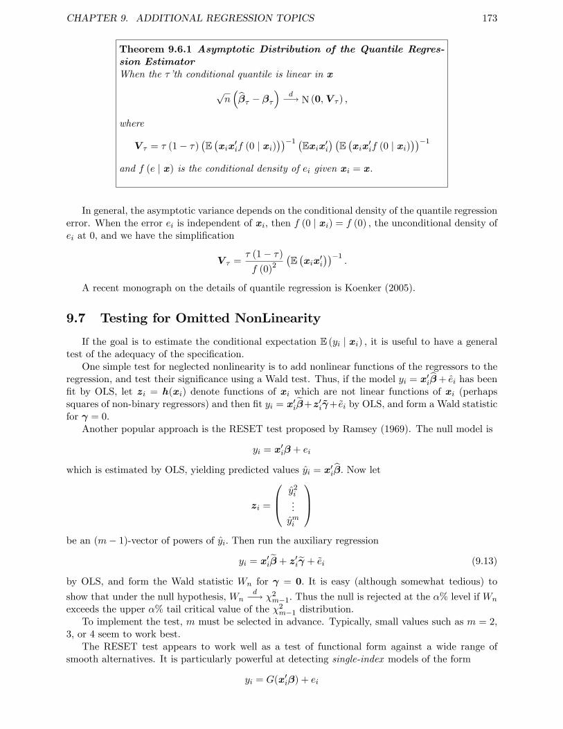
CHAPTER 9. ADDITIONAL REGRESSION TOPICS 173
Theorem 9.6.1 Asymptotic Distribution of the Quantile Regres-sion EstimatorWhen the τ’th conditional quantile is linear in x
√n(βτ − βτ
)d−→ N (0,V τ ) ,
where
V τ = τ (1− τ)(E(xix
′if (0 | xi)
))−1 (Exix′i) (E (xix′if (0 | xi)))−1
and f (e | x) is the conditional density of ei given xi = x.
In general, the asymptotic variance depends on the conditional density of the quantile regressionerror. When the error ei is independent of xi, then f (0 | xi) = f (0) , the unconditional density ofei at 0, and we have the simplification
V τ =τ (1− τ)
f (0)2
(E(xix
′i
))−1.
A recent monograph on the details of quantile regression is Koenker (2005).
9.7 Testing for Omitted NonLinearity
If the goal is to estimate the conditional expectation E (yi | xi) , it is useful to have a generaltest of the adequacy of the specification.
One simple test for neglected nonlinearity is to add nonlinear functions of the regressors to theregression, and test their significance using a Wald test. Thus, if the model yi = x′iβ+ ei has beenfit by OLS, let zi = h(xi) denote functions of xi which are not linear functions of xi (perhapssquares of non-binary regressors) and then fit yi = x′iβ+z′iγ+ ei by OLS, and form a Wald statisticfor γ = 0.
Another popular approach is the RESET test proposed by Ramsey (1969). The null model is
yi = x′iβ + ei
which is estimated by OLS, yielding predicted values yi = x′iβ. Now let
zi =
y2i...ymi
be an (m− 1)-vector of powers of yi. Then run the auxiliary regression
yi = x′iβ + z′iγ + ei (9.13)
by OLS, and form the Wald statistic Wn for γ = 0. It is easy (although somewhat tedious) to
show that under the null hypothesis, Wnd−→ χ2
m−1. Thus the null is rejected at the α% level if Wn
exceeds the upper α% tail critical value of the χ2m−1 distribution.
To implement the test, m must be selected in advance. Typically, small values such as m = 2,3, or 4 seem to work best.
The RESET test appears to work well as a test of functional form against a wide range ofsmooth alternatives. It is particularly powerful at detecting single-index models of the form
yi = G(x′iβ) + ei
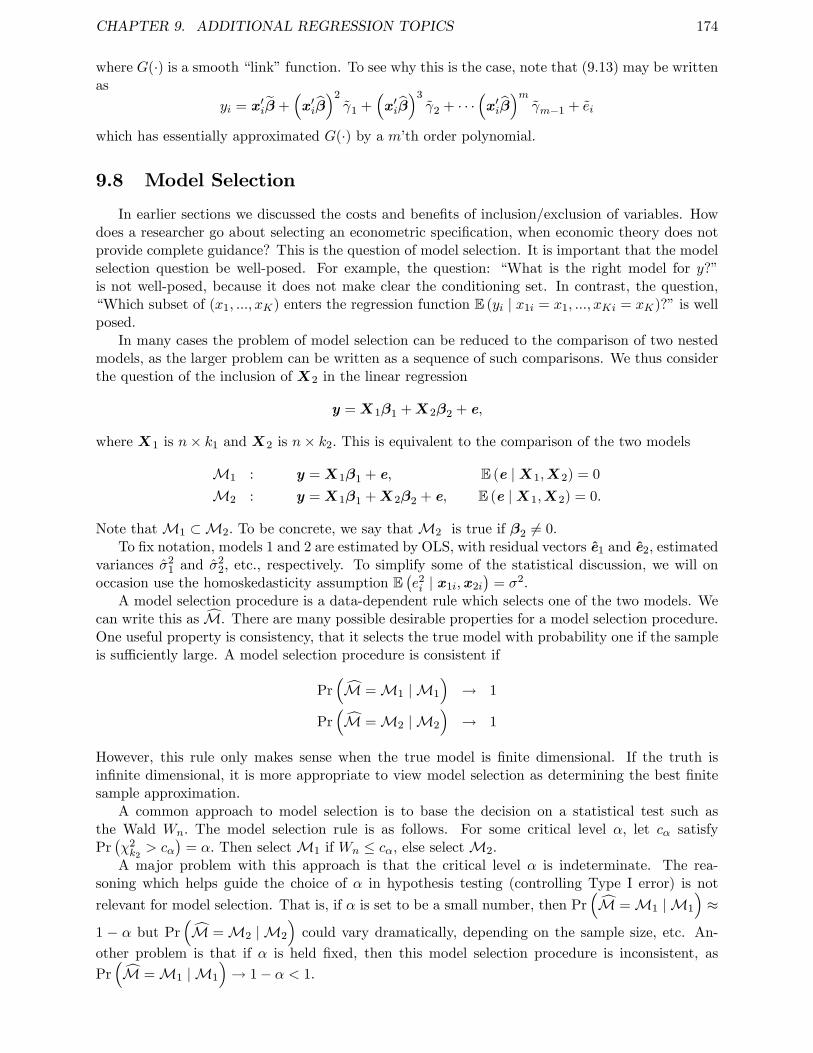
CHAPTER 9. ADDITIONAL REGRESSION TOPICS 174
where G(·) is a smooth “link”function. To see why this is the case, note that (9.13) may be writtenas
yi = x′iβ +(x′iβ
)2γ1 +
(x′iβ
)3γ2 + · · ·
(x′iβ
)mγm−1 + ei
which has essentially approximated G(·) by a m’th order polynomial.
9.8 Model Selection
In earlier sections we discussed the costs and benefits of inclusion/exclusion of variables. Howdoes a researcher go about selecting an econometric specification, when economic theory does notprovide complete guidance? This is the question of model selection. It is important that the modelselection question be well-posed. For example, the question: “What is the right model for y?”is not well-posed, because it does not make clear the conditioning set. In contrast, the question,“Which subset of (x1, ..., xK) enters the regression function E (yi | x1i = x1, ..., xKi = xK)?”is wellposed.
In many cases the problem of model selection can be reduced to the comparison of two nestedmodels, as the larger problem can be written as a sequence of such comparisons. We thus considerthe question of the inclusion of X2 in the linear regression
y = X1β1 +X2β2 + e,
where X1 is n× k1 and X2 is n× k2. This is equivalent to the comparison of the two models
M1 : y = X1β1 + e, E (e |X1,X2) = 0
M2 : y = X1β1 +X2β2 + e, E (e |X1,X2) = 0.
Note thatM1 ⊂M2. To be concrete, we say thatM2 is true if β2 6= 0.To fix notation, models 1 and 2 are estimated by OLS, with residual vectors e1 and e2, estimated
variances σ21 and σ
22, etc., respectively. To simplify some of the statistical discussion, we will on
occasion use the homoskedasticity assumption E(e2i | x1i,x2i
)= σ2.
A model selection procedure is a data-dependent rule which selects one of the two models. Wecan write this as M. There are many possible desirable properties for a model selection procedure.One useful property is consistency, that it selects the true model with probability one if the sampleis suffi ciently large. A model selection procedure is consistent if
Pr(M =M1 | M1
)→ 1
Pr(M =M2 | M2
)→ 1
However, this rule only makes sense when the true model is finite dimensional. If the truth isinfinite dimensional, it is more appropriate to view model selection as determining the best finitesample approximation.
A common approach to model selection is to base the decision on a statistical test such asthe Wald Wn. The model selection rule is as follows. For some critical level α, let cα satisfyPr(χ2k2> cα
)= α. Then selectM1 if Wn ≤ cα, else selectM2.
A major problem with this approach is that the critical level α is indeterminate. The rea-soning which helps guide the choice of α in hypothesis testing (controlling Type I error) is not
relevant for model selection. That is, if α is set to be a small number, then Pr(M =M1 | M1
)≈
1 − α but Pr(M =M2 | M2
)could vary dramatically, depending on the sample size, etc. An-
other problem is that if α is held fixed, then this model selection procedure is inconsistent, as
Pr(M =M1 | M1
)→ 1− α < 1.
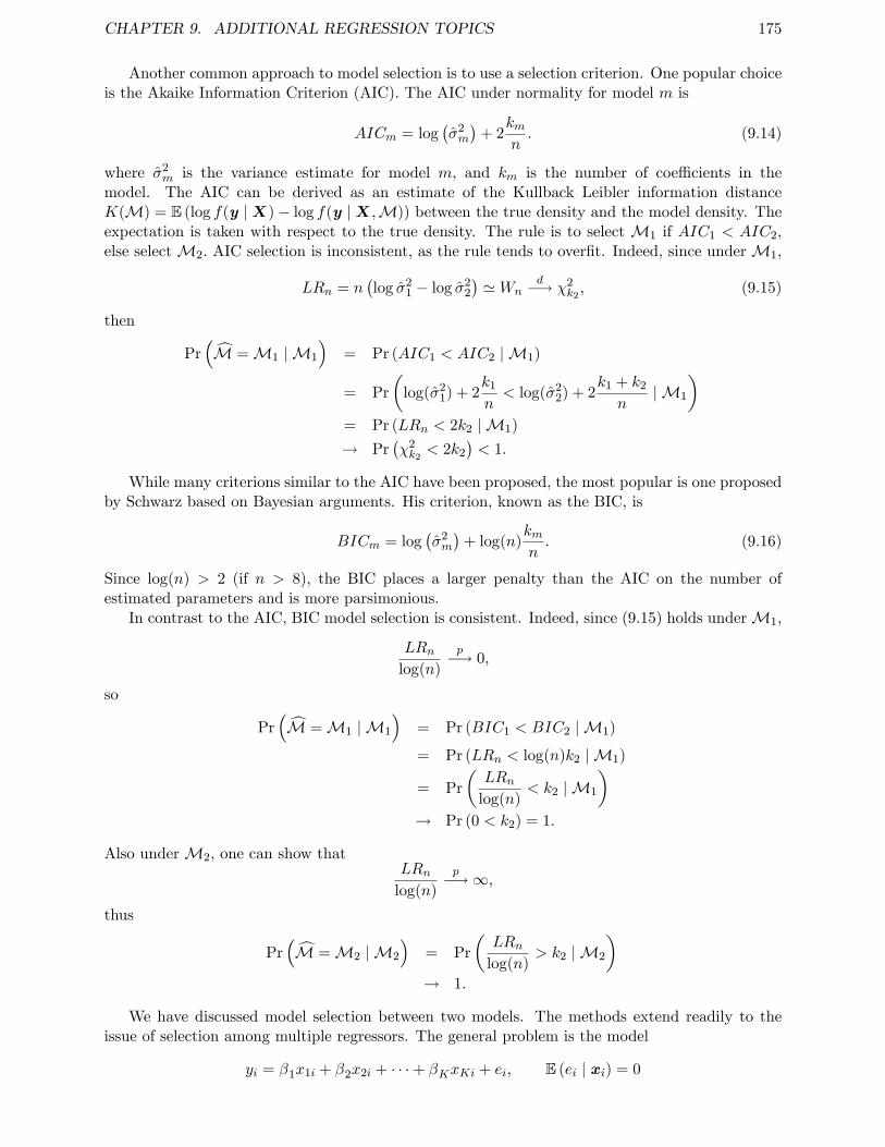
CHAPTER 9. ADDITIONAL REGRESSION TOPICS 175
Another common approach to model selection is to use a selection criterion. One popular choiceis the Akaike Information Criterion (AIC). The AIC under normality for model m is
AICm = log(σ2m
)+ 2
kmn. (9.14)
where σ2m is the variance estimate for model m, and km is the number of coeffi cients in the
model. The AIC can be derived as an estimate of the Kullback Leibler information distanceK(M) = E (log f(y |X)− log f(y |X,M)) between the true density and the model density. Theexpectation is taken with respect to the true density. The rule is to select M1 if AIC1 < AIC2,else selectM2. AIC selection is inconsistent, as the rule tends to overfit. Indeed, since underM1,
LRn = n(log σ2
1 − log σ22
)'Wn
d−→ χ2k2 , (9.15)
then
Pr(M =M1 | M1
)= Pr (AIC1 < AIC2 | M1)
= Pr
(log(σ2
1) + 2k1
n< log(σ2
2) + 2k1 + k2
n| M1
)= Pr (LRn < 2k2 | M1)
→ Pr(χ2k2 < 2k2
)< 1.
While many criterions similar to the AIC have been proposed, the most popular is one proposedby Schwarz based on Bayesian arguments. His criterion, known as the BIC, is
BICm = log(σ2m
)+ log(n)
kmn. (9.16)
Since log(n) > 2 (if n > 8), the BIC places a larger penalty than the AIC on the number ofestimated parameters and is more parsimonious.
In contrast to the AIC, BIC model selection is consistent. Indeed, since (9.15) holds underM1,
LRnlog(n)
p−→ 0,
so
Pr(M =M1 | M1
)= Pr (BIC1 < BIC2 | M1)
= Pr (LRn < log(n)k2 | M1)
= Pr
(LRn
log(n)< k2 | M1
)→ Pr (0 < k2) = 1.
Also underM2, one can show thatLRn
log(n)
p−→∞,
thus
Pr(M =M2 | M2
)= Pr
(LRn
log(n)> k2 | M2
)→ 1.
We have discussed model selection between two models. The methods extend readily to theissue of selection among multiple regressors. The general problem is the model
yi = β1x1i + β2x2i + · · ·+ βKxKi + ei, E (ei | xi) = 0
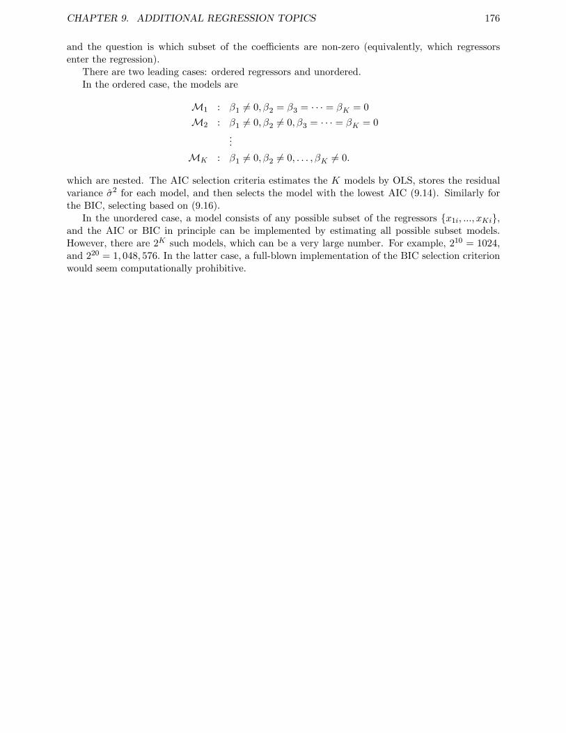
CHAPTER 9. ADDITIONAL REGRESSION TOPICS 176
and the question is which subset of the coeffi cients are non-zero (equivalently, which regressorsenter the regression).
There are two leading cases: ordered regressors and unordered.In the ordered case, the models are
M1 : β1 6= 0, β2 = β3 = · · · = βK = 0
M2 : β1 6= 0, β2 6= 0, β3 = · · · = βK = 0
...
MK : β1 6= 0, β2 6= 0, . . . , βK 6= 0.
which are nested. The AIC selection criteria estimates the K models by OLS, stores the residualvariance σ2 for each model, and then selects the model with the lowest AIC (9.14). Similarly forthe BIC, selecting based on (9.16).
In the unordered case, a model consists of any possible subset of the regressors x1i, ..., xKi,and the AIC or BIC in principle can be implemented by estimating all possible subset models.However, there are 2K such models, which can be a very large number. For example, 210 = 1024,and 220 = 1, 048, 576. In the latter case, a full-blown implementation of the BIC selection criterionwould seem computationally prohibitive.
CHAPTER 9. ADDITIONAL REGRESSION TOPICS 177
Exercises
Exercise 9.1 The data file cps78.dat contains 550 observations on 20 variables taken from theMay 1978 current population survey. Variables are listed in the file cps78.pdf. The goal of theexercise is to estimate a model for the log of earnings (variable LNWAGE) as a function of theconditioning variables.
(a) Start by an OLS regression of LNWAGE on the other variables. Report coeffi cient estimatesand standard errors.
(b) Consider augmenting the model by squares and/or cross-products of the conditioning vari-ables. Estimate your selected model and report the results.
(c) Are there any variables which seem to be unimportant as a determinant of wages? You mayre-estimate the model without these variables, if desired.
(d) Test whether the error variance is different for men and women. Interpret.
(e) Test whether the error variance is different for whites and nonwhites. Interpret.
(f) Construct a model for the conditional variance. Estimate such a model, test for generalheteroskedasticity and report the results.
(g) Using this model for the conditional variance, re-estimate the model from part (c) usingFGLS. Report the results.
(h) Do the OLS and FGLS estimates differ greatly? Note any interesting differences.
(i) Compare the estimated standard errors. Note any interesting differences.
Exercise 9.2 In the homoskedastic regression model y = Xβ + e with E(ei | xi) = 0 and E(e2i |
xi) = σ2, suppose β is the OLS estimate of β with covariance matrix V , based on a sample ofsize n. Let σ2 be the estimate of σ2. You wish to forecast an out-of-sample value of yn+1 giventhat xn+1 = x. Thus the available information is the sample (y,X), the estimates (β, V , σ2), theresiduals e, and the out-of-sample value of the regressors, xn+1.
(a) Find a point forecast of yn+1.
(b) Find an estimate of the variance of this forecast.
Exercise 9.3 Suppose that yi = g(xi,θ)+ei with E (ei | xi) = 0, θ is the NLLS estimator, and V is
the estimate of var(θ). You are interested in the conditional mean function E (yi | xi = x) = g(x)
at some x. Find an asymptotic 95% confidence interval for g(x).
Exercise 9.4 For any predictor g(xi) for yi, the mean absolute error (MAE) is
E |yi − g(xi)| .
Show that the function g(x) which minimizes the MAE is the conditional median m (x) = med(yi |xi).
Exercise 9.5 Defineg(u) = τ − 1 (u < 0)
where 1 (·) is the indicator function (takes the value 1 if the argument is true, else equals zero).Let θ satisfy Eg(yi − θ) = 0. Is θ a quantile of the distribution of yi?
CHAPTER 9. ADDITIONAL REGRESSION TOPICS 178
Exercise 9.6 Verify equation (9.11).
Exercise 9.7 In Exercise 8.4, you estimated a cost function on a cross-section of electric companies.The equation you estimated was
log TCi = β1 + β2 logQi + β3 logPLi + β4 logPKi + β5 logPFi + ei. (9.17)
(a) Following Nerlove, add the variable (logQi)2 to the regression. Do so. Assess the merits of
this new specification using (i) a hypothesis test; (ii) AIC criterion; (iii) BIC criterion. Doyou agree with this modification?
(b) Now try a non-linear specification. Consider model (9.17) plus the extra term β6zi, where
zi = logQi (1 + exp (− (logQi − β7)))−1 .
In addition, impose the restriction β3 + β4 + β5 = 1. This model is called a smooth thresholdmodel. For values of logQi much below β7, the variable logQi has a regression slope of β2.For values much above β7, the regression slope is β2 + β6, and the model imposes a smoothtransition between these regimes. The model is non-linear because of the parameter β7.
The model works best when β7 is selected so that several values (in this example, at least10 to 15) of logQi are both below and above β7. Examine the data and pick an appropriaterange for β7.
(c) Estimate the model by non-linear least squares. I recommend the concentration method:Pick 10 (or more or you like) values of β7 in this range. For each value of β7, calculate ziand estimate the model by OLS. Record the sum of squared errors, and find the value of β7
for which the sum of squared errors is minimized.
(d) Calculate standard errors for all the parameters (β1, ..., β7).
Chapter 10
The Bootstrap
10.1 Definition of the Bootstrap
Let F denote a distribution function for the population of observations (yi,xi) . Let
Tn = Tn ((y1,x1) , ..., (yn,xn) , F )
be a statistic of interest, for example an estimator θ or a t-statistic(θ − θ
)/s(θ). Note that we
write Tn as possibly a function of F . For example, the t-statistic is a function of the parameter θwhich itself is a function of F.
The exact CDF of Tn when the data are sampled from the distribution F is
Gn(u, F ) = Pr(Tn ≤ u | F )
In general, Gn(u, F ) depends on F, meaning that G changes as F changes.Ideally, inference would be based on Gn(u, F ). This is generally impossible since F is unknown.Asymptotic inference is based on approximating Gn(u, F ) with G(u, F ) = limn→∞Gn(u, F ).
When G(u, F ) = G(u) does not depend on F, we say that Tn is asymptotically pivotal and use thedistribution function G(u) for inferential purposes.
In a seminal contribution, Efron (1979) proposed the bootstrap, which makes a different ap-proximation. The unknown F is replaced by a consistent estimate Fn (one choice is discussed inthe next section). Plugged into Gn(u, F ) we obtain
G∗n(u) = Gn(u, Fn). (10.1)
We call G∗n the bootstrap distribution. Bootstrap inference is based on G∗n(u).
Let (y∗i ,x∗i ) denote random variables with the distribution Fn. A random sample from this dis-
tribution is called the bootstrap data. The statistic T ∗n = Tn ((y∗1,x∗1) , ..., (y∗n,x
∗n) , Fn) constructed
on this sample is a random variable with distribution G∗n. That is, Pr(T ∗n ≤ u) = G∗n(u). We callT ∗n the bootstrap statistic. The distribution of T
∗n is identical to that of Tn when the true CDF is
Fn rather than F.The bootstrap distribution is itself random, as it depends on the sample through the estimator
Fn.In the next sections we describe computation of the bootstrap distribution.
10.2 The Empirical Distribution Function
Recall that F (y,x) = Pr (yi ≤ y,xi ≤ x) = E (1 (yi ≤ y) 1 (xi ≤ x)) , where 1(·) is the indicatorfunction. This is a population moment. The method of moments estimator is the corresponding
179
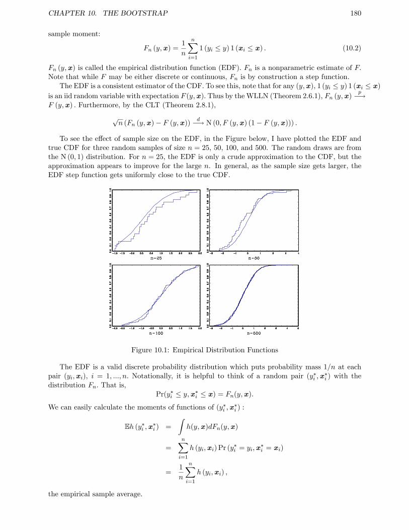
CHAPTER 10. THE BOOTSTRAP 180
sample moment:
Fn (y,x) =1
n
n∑i=1
1 (yi ≤ y) 1 (xi ≤ x) . (10.2)
Fn (y,x) is called the empirical distribution function (EDF). Fn is a nonparametric estimate of F.Note that while F may be either discrete or continuous, Fn is by construction a step function.
The EDF is a consistent estimator of the CDF. To see this, note that for any (y,x), 1 (yi ≤ y) 1 (xi ≤ x)
is an iid random variable with expectation F (y,x). Thus by theWLLN (Theorem 2.6.1), Fn (y,x)p−→
F (y,x) . Furthermore, by the CLT (Theorem 2.8.1),
√n (Fn (y,x)− F (y,x))
d−→ N (0, F (y,x) (1− F (y,x))) .
To see the effect of sample size on the EDF, in the Figure below, I have plotted the EDF andtrue CDF for three random samples of size n = 25, 50, 100, and 500. The random draws are fromthe N (0, 1) distribution. For n = 25, the EDF is only a crude approximation to the CDF, but theapproximation appears to improve for the large n. In general, as the sample size gets larger, theEDF step function gets uniformly close to the true CDF.
Figure 10.1: Empirical Distribution Functions
The EDF is a valid discrete probability distribution which puts probability mass 1/n at eachpair (yi,xi), i = 1, ..., n. Notationally, it is helpful to think of a random pair (y∗i ,x
∗i ) with the
distribution Fn. That is,Pr(y∗i ≤ y,x∗i ≤ x) = Fn(y,x).
We can easily calculate the moments of functions of (y∗i ,x∗i ) :
Eh (y∗i ,x∗i ) =
∫h(y,x)dFn(y,x)
=n∑i=1
h (yi,xi) Pr (y∗i = yi,x∗i = xi)
=1
n
n∑i=1
h (yi,xi) ,
the empirical sample average.
CHAPTER 10. THE BOOTSTRAP 181
10.3 Nonparametric Bootstrap
The nonparametric bootstrap is obtained when the bootstrap distribution (10.1) is definedusing the EDF (10.2) as the estimate Fn of F.
Since the EDF Fn is a multinomial (with n support points), in principle the distributionG∗n couldbe calculated by direct methods. However, as there are
(2n−1n
)possible samples (y∗1,x∗1) , ..., (y∗n,x
∗n),
such a calculation is computationally infeasible. The popular alternative is to use simulation to ap-proximate the distribution. The algorithm is identical to our discussion of Monte Carlo simulation,with the following points of clarification:
• The sample size n used for the simulation is the same as the sample size.
• The random vectors (y∗i ,x∗i ) are drawn randomly from the empirical distribution. This is
equivalent to sampling a pair (yi,xi) randomly from the sample.
The bootstrap statistic T ∗n = Tn ((y∗1,x∗1) , ..., (y∗n,x
∗n) , Fn) is calculated for each bootstrap sam-
ple. This is repeated B times. B is known as the number of bootstrap replications. A theoryfor the determination of the number of bootstrap replications B has been developed by Andrewsand Buchinsky (2000). It is desirable for B to be large, so long as the computational costs arereasonable. B = 1000 typically suffi ces.
When the statistic Tn is a function of F, it is typically through dependence on a parameter.
For example, the t-ratio(θ − θ
)/s(θ) depends on θ. As the bootstrap statistic replaces F with
Fn, it similarly replaces θ with θn, the value of θ implied by Fn. Typically θn = θ, the parameterestimate. (When in doubt use θ.)
Sampling from the EDF is particularly easy. Since Fn is a discrete probability distributionputting probability mass 1/n at each sample point, sampling from the EDF is equivalent to randomsampling a pair (yi,xi) from the observed data with replacement. In consequence, a bootstrapsample (y∗1,x∗1) , ..., (y∗n,x
∗n) will necessarily have some ties and multiple values, which is generally
not a problem.
10.4 Bootstrap Estimation of Bias and Variance
The bias of θ is τn = E(θ − θ0). Let Tn(θ) = θ − θ. Then τn = E(Tn(θ0)). The bootstrapcounterparts are θ
∗= θ((y∗1,x
∗1) , ..., (y∗n,x
∗n)) and T ∗n = θ
∗ − θn = θ∗ − θ. The bootstrap estimate
of τn isτ∗n = E(T ∗n).
If this is calculated by the simulation described in the previous section, the estimate of τ∗n is
τ∗n =1
B
B∑b=1
T ∗nb
=1
B
B∑b=1
θ∗b − θ
= θ∗ − θ.
If θ is biased, it might be desirable to construct a biased-corrected estimator (one with reducedbias). Ideally, this would be
θ = θ − τn,
CHAPTER 10. THE BOOTSTRAP 182
but τn is unknown. The (estimated) bootstrap biased-corrected estimator is
θ∗
= θ − τ∗n= θ − (θ
∗ − θ)
= 2θ − θ∗.
Note, in particular, that the biased-corrected estimator is not θ∗. Intuitively, the bootstrap makes
the following experiment. Suppose that θ is the truth. Then what is the average value of θ
calculated from such samples? The answer is θ∗. If this is lower than θ, this suggests that the
estimator is downward-biased, so a biased-corrected estimator of θ should be larger than θ, and the
best guess is the difference between θ and θ∗. Similarly if θ
∗is higher than θ, then the estimator is
upward-biased and the biased-corrected estimator should be lower than θ.Let Tn = θ. The variance of θ is
Vn = E(Tn − ETn)2.
Let T ∗n = θ∗. It has variance
V ∗n = E(T ∗n − ET ∗n)2.
The simulation estimate is
V ∗n =1
B
B∑b=1
(θ∗b − θ
∗)2
.
A bootstrap standard error for θ is the square root of the bootstrap estimate of variance,
s∗(θ) =
√V ∗n .
While this standard error may be calculated and reported, it is not clear if it is useful. Theprimary use of asymptotic standard errors is to construct asymptotic confidence intervals, which arebased on the asymptotic normal approximation to the t-ratio. However, the use of the bootstrappresumes that such asymptotic approximations might be poor, in which case the normal approxi-mation is suspected. It appears superior to calculate bootstrap confidence intervals, and we turnto this next.
10.5 Percentile Intervals
For a distribution function Gn(u, F ), let qn(α, F ) denote its quantile function. This is thefunction which solves
Gn(qn(α, F ), F ) = α.
[When Gn(u, F ) is discrete, qn(α, F ) may be non-unique, but we will ignore such complications.]Let qn(α) denote the quantile function of the true sampling distribution, and q∗n(α) = qn(α, Fn)denote the quantile function of the bootstrap distribution. Note that this function will changedepending on the underlying statistic Tn whose distribution is Gn.
Let Tn = θ, an estimate of a parameter of interest. In (1− α)% of samples, θ lies in the region[qn(α/2), qn(1− α/2)]. This motivates a confidence interval proposed by Efron:
C1 = [q∗n(α/2), q∗n(1− α/2)].
This is often called the percentile confidence interval.Computationally, the quantile q∗n(α) is estimated by q∗n(α), the α’th sample quantile of the
simulated statistics T ∗n1, ..., T∗nB, as discussed in the section on Monte Carlo simulation. The
(1− α)% Efron percentile interval is then [q∗n(α/2), q∗n(1− α/2)].
CHAPTER 10. THE BOOTSTRAP 183
The interval C1 is a popular bootstrap confidence interval often used in empirical practice. Thisis because it is easy to compute, simple to motivate, was popularized by Efron early in the historyof the bootstrap, and also has the feature that it is translation invariant. That is, if we defineφ = f(θ) as the parameter of interest for a monotonically increasing function f, then percentilemethod applied to this problem will produce the confidence interval [f(q∗n(α/2)), f(q∗n(1−α/2))],which is a naturally good property.
However, as we show now, C1 is in a deep sense very poorly motivated.It will be useful if we introduce an alternative definition C1. Let Tn(θ) = θ − θ and let qn(α)
be the quantile function of its distribution. (These are the original quantiles, with θ subtracted.)Then C1 can alternatively be written as
C1 = [θ + q∗n(α/2), θ + q∗n(1− α/2)].
This is a bootstrap estimate of the “ideal”confidence interval
C01 = [θ + qn(α/2), θ + qn(1− α/2)].
The latter has coverage probability
Pr(θ0 ∈ C0
1
)= Pr
(θ + qn(α/2) ≤ θ0 ≤ θ + qn(1− α/2)
)= Pr
(−qn(1− α/2) ≤ θ − θ0 ≤ −qn(α/2)
)= Gn(−qn(α/2), F0)−Gn(−qn(1− α/2), F0)
which generally is not 1−α! There is one important exception. If θ−θ0 has a symmetric distribution,then Gn(−u, F0) = 1−Gn(u, F0), so
Pr(θ0 ∈ C0
1
)= Gn(−qn(α/2), F0)−Gn(−qn(1− α/2), F0)
= (1−Gn(qn(α/2), F0))− (1−Gn(qn(1− α/2), F0))
=(
1− α
2
)−(
1−(
1− α
2
))= 1− α
and this idealized confidence interval is accurate. Therefore, C01 and C1 are designed for the case
that θ has a symmetric distribution about θ0.When θ does not have a symmetric distribution, C1 may perform quite poorly.However, by the translation invariance argument presented above, it also follows that if there
exists some monotonically increasing transformation f(·) such that f(θ) is symmetrically distributedabout f(θ0), then the idealized percentile bootstrap method will be accurate.
Based on these arguments, many argue that the percentile interval should not be used unlessthe sampling distribution is close to unbiased and symmetric.
The problems with the percentile method can be circumvented, at least in principle, by analternative method.
Let Tn(θ) = θ − θ. Then
1− α = Pr (qn(α/2) ≤ Tn(θ0) ≤ qn(1− α/2))
= Pr(θ − qn(1− α/2) ≤ θ0 ≤ θ − qn(α/2)
),
so an exact (1− α)% confidence interval for θ0 would be
C02 = [θ − qn(1− α/2), θ − qn(α/2)].
This motivates a bootstrap analog
C2 = [θ − q∗n(1− α/2), θ − q∗n(α/2)].
CHAPTER 10. THE BOOTSTRAP 184
Notice that generally this is very different from the Efron interval C1! They coincide in the specialcase that G∗n(u) is symmetric about θ, but otherwise they differ.
Computationally, this interval can be estimated from a bootstrap simulation by sorting the
bootstrap statistics T ∗n =(θ∗ − θ
), which are centered at the sample estimate θ. These are sorted
to yield the quantile estimates q∗n(.025) and q∗n(.975). The 95% confidence interval is then [θ −q∗n(.975), θ − q∗n(.025)].
This confidence interval is discussed in most theoretical treatments of the bootstrap, but is notwidely used in practice.
10.6 Percentile-t Equal-Tailed Interval
Suppose we want to test H0 : θ = θ0 against H1 : θ < θ0 at size α. We would set Tn(θ) =(θ − θ
)/s(θ) and reject H0 in favor of H1 if Tn(θ0) < c, where c would be selected so that
Pr (Tn(θ0) < c) = α.
Thus c = qn(α). Since this is unknown, a bootstrap test replaces qn(α) with the bootstrap estimateq∗n(α), and the test rejects if Tn(θ0) < q∗n(α).
Similarly, if the alternative is H1 : θ > θ0, the bootstrap test rejects if Tn(θ0) > q∗n(1− α).Computationally, these critical values can be estimated from a bootstrap simulation by sorting
the bootstrap t-statistics T ∗n =(θ∗ − θ
)/s(θ
∗). Note, and this is important, that the bootstrap test
statistic is centered at the estimate θ, and the standard error s(θ∗) is calculated on the bootstrap
sample. These t-statistics are sorted to find the estimated quantiles q∗n(α) and/or q∗n(1− α).
Let Tn(θ) =(θ − θ
)/s(θ). Then taking the intersection of two one-sided intervals,
1− α = Pr (qn(α/2) ≤ Tn(θ0) ≤ qn(1− α/2))
= Pr(qn(α/2) ≤
(θ − θ0
)/s(θ) ≤ qn(1− α/2)
)= Pr
(θ − s(θ)qn(1− α/2) ≤ θ0 ≤ θ − s(θ)qn(α/2)
),
so an exact (1− α)% confidence interval for θ0 would be
C03 = [θ − s(θ)qn(1− α/2), θ − s(θ)qn(α/2)].
This motivates a bootstrap analog
C3 = [θ − s(θ)q∗n(1− α/2), θ − s(θ)q∗n(α/2)].
This is often called a percentile-t confidence interval. It is equal-tailed or central since the probabilitythat θ0 is below the left endpoint approximately equals the probability that θ0 is above the rightendpoint, each α/2.
Computationally, this is based on the critical values from the one-sided hypothesis tests, dis-cussed above.
10.7 Symmetric Percentile-t Intervals
Suppose we want to test H0 : θ = θ0 against H1 : θ 6= θ0 at size α. We would set Tn(θ) =(θ − θ
)/s(θ) and reject H0 in favor of H1 if |Tn(θ0)| > c, where c would be selected so that
Pr (|Tn(θ0)| > c) = α.
CHAPTER 10. THE BOOTSTRAP 185
Note that
Pr (|Tn(θ0)| < c) = Pr (−c < Tn(θ0) < c)
= Gn(c)−Gn(−c)≡ Gn(c),
which is a symmetric distribution function. The ideal critical value c = qn(α) solves the equation
Gn(qn(α)) = 1− α.
Equivalently, qn(α) is the 1− α quantile of the distribution of |Tn(θ0)| .The bootstrap estimate is q∗n(α), the 1 − α quantile of the distribution of |T ∗n | , or the number
which solves the equation
G∗n(q∗n(α)) = G∗n(q∗n(α))−G∗n(−q∗n(α)) = 1− α.
Computationally, q∗n(α) is estimated from a bootstrap simulation by sorting the bootstrap t-
statistics |T ∗n | =∣∣∣θ∗ − θ∣∣∣ /s(θ∗), and taking the upper α% quantile. The bootstrap test rejects if
|Tn(θ0)| > q∗n(α).Let
C4 = [θ − s(θ)q∗n(α), θ + s(θ)q∗n(α)],
where q∗n(α) is the bootstrap critical value for a two-sided hypothesis test. C4 is called the symmetricpercentile-t interval. It is designed to work well since
Pr (θ0 ∈ C4) = Pr(θ − s(θ)q∗n(α) ≤ θ0 ≤ θ + s(θ)q∗n(α)
)= Pr (|Tn(θ0)| < q∗n(α))
' Pr (|Tn(θ0)| < qn(α))
= 1− α.
If θ is a vector, then to test H0 : θ = θ0 against H1 : θ 6= θ0 at size α, we would use a Waldstatistic
Wn(θ) = n(θ − θ
)′V−1θ
(θ − θ
)or some other asymptotically chi-square statistic. Thus here Tn(θ) = Wn(θ). The ideal test rejectsif Wn ≥ qn(α), where qn(α) is the (1− α)% quantile of the distribution of Wn. The bootstrap testrejects if Wn ≥ q∗n(α), where q∗n(α) is the (1− α)% quantile of the distribution of
W ∗n = n(θ∗ − θ
)′V∗−1θ
(θ∗ − θ
).
Computationally, the critical value q∗n(α) is found as the quantile from simulated values of W ∗n .
Note in the simulation that the Wald statistic is a quadratic form in(θ∗ − θ
), not
(θ∗ − θ0
).
[This is a typical mistake made by practitioners.]
10.8 Asymptotic Expansions
Let Tn ∈ R be a statistic such that
Tnd−→ N(0, σ2). (10.3)
CHAPTER 10. THE BOOTSTRAP 186
In some cases, such as when Tn is a t-ratio, then σ2 = 1. In other cases σ2 is unknown. Equivalently,writing Tn ∼ Gn(u, F ) then for each u and F
limn→∞
Gn(u, F ) = Φ(uσ
),
orGn(u, F ) = Φ
(uσ
)+ o (1) . (10.4)
While (10.4) says that Gn converges to Φ(uσ
)as n→∞, it says nothing, however, about the rate
of convergence, or the size of the divergence for any particular sample size n. A better asymptoticapproximation may be obtained through an asymptotic expansion.
The following notation will be helpful. Let an be a sequence.
Definition 10.8.1 an = o(1) if an → 0 as n→∞
Definition 10.8.2 an = O(1) if |an| is uniformly bounded.
Definition 10.8.3 an = o(n−r) if nr |an| → 0 as n→∞.
Basically, an = O(n−r) if it declines to zero like n−r.We say that a function g(u) is even if g(−u) = g(u), and a function h(u) is odd if h(−u) = −h(u).
The derivative of an even function is odd, and vice-versa.
Theorem 10.8.1 Under regularity conditions and (10.3),
Gn(u, F ) = Φ(uσ
)+
1
n1/2g1(u, F ) +
1
ng2(u, F ) +O(n−3/2)
uniformly over u, where g1 is an even function of u, and g2 is an oddfunction of u. Moreover, g1 and g2 are differentiable functions of u andcontinuous in F relative to the supremum norm on the space of distributionfunctions.
The expansion in Theorem 10.8.1 is often called an Edgeworth expansion.We can interpret Theorem 10.8.1 as follows. First, Gn(u, F ) converges to the normal limit at
rate n1/2. To a second order of approximation,
Gn(u, F ) ≈ Φ(uσ
)+ n−1/2g1(u, F ).
Since the derivative of g1 is odd, the density function is skewed. To a third order of approximation,
Gn(u, F ) ≈ Φ(uσ
)+ n−1/2g1(u, F ) + n−1g2(u, F )
which adds a symmetric non-normal component to the approximate density (for example, addingleptokurtosis).
CHAPTER 10. THE BOOTSTRAP 187
[Side Note: When Tn =√n(Xn − µ
)/σ, a standardized sample mean, then
g1(u) = −1
6κ3
(u2 − 1
)φ(u)
g2(u) = −(
1
24κ4
(u3 − 3u
)+
1
72κ2
3
(u5 − 10u3 + 15u
))φ(u)
where φ(u) is the standard normal pdf, and
κ3 = E (X − µ)3 /σ3
κ4 = E (X − µ)4 /σ4 − 3
the standardized skewness and excess kurtosis of the distribution of X. Note that when κ3 = 0and κ4 = 0, then g1 = 0 and g2 = 0, so the second-order Edgeworth expansion corresponds to thenormal distribution.]
Francis Edgeworth
Francis Ysidro Edgeworth (1845-1926) of Ireland, founding editor of the Economic Journal,was a profound economic and statistical theorist, developing the theories of indifferencecurves and asymptotic expansions. He also could be viewed as the first econometrician dueto his early use of mathematical statistics in the study of economic data.
10.9 One-Sided Tests
Using the expansion of Theorem 10.8.1, we can assess the accuracy of one-sided hypothesis testsand confidence regions based on an asymptotically normal t-ratio Tn. An asymptotic test is basedon Φ(u).
To the second order, the exact distribution is
Pr (Tn < u) = Gn(u, F0) = Φ(u) +1
n1/2g1(u, F0) +O(n−1)
since σ = 1. The difference is
Φ(u)−Gn(u, F0) =1
n1/2g1(u, F0) +O(n−1)
= O(n−1/2),
so the order of the error is O(n−1/2).A bootstrap test is based on G∗n(u), which from Theorem 10.8.1 has the expansion
G∗n(u) = Gn(u, Fn) = Φ(u) +1
n1/2g1(u, Fn) +O(n−1).
Because Φ(u) appears in both expansions, the difference between the bootstrap distribution andthe true distribution is
G∗n(u)−Gn(u, F0) =1
n1/2(g1(u, Fn)− g1(u, F0)) +O(n−1).
CHAPTER 10. THE BOOTSTRAP 188
Since Fn converges to F at rate√n, and g1 is continuous with respect to F, the difference
(g1(u, Fn)− g1(u, F0)) converges to 0 at rate√n. Heuristically,
g1(u, Fn)− g1(u, F0) ≈ ∂
∂Fg1(u, F0) (Fn − F0)
= O(n−1/2),
The “derivative” ∂∂F g1(u, F ) is only heuristic, as F is a function. We conclude that
G∗n(u)−Gn(u, F0) = O(n−1),
orPr (T ∗n ≤ u) = Pr (Tn ≤ u) +O(n−1),
which is an improved rate of convergence over the asymptotic test (which converged at rateO(n−1/2)). This rate can be used to show that one-tailed bootstrap inference based on the t-ratio achieves a so-called asymptotic refinement —the Type I error of the test converges at a fasterrate than an analogous asymptotic test.
10.10 Symmetric Two-Sided Tests
If a random variable y has distribution function H(u) = Pr(y ≤ u), then the random variable|y| has distribution function
H(u) = H(u)−H(−u)
since
Pr (|y| ≤ u) = Pr (−u ≤ y ≤ u)
= Pr (y ≤ u)− Pr (y ≤ −u)
= H(u)−H(−u).
For example, if Z ∼ N(0, 1), then |Z| has distribution function
Φ(u) = Φ(u)− Φ(−u) = 2Φ(u)− 1.
Similarly, if Tn has exact distribution Gn(u, F ), then |Tn| has the distribution function
Gn(u, F ) = Gn(u, F )−Gn(−u, F ).
A two-sided hypothesis test rejects H0 for large values of |Tn| . Since Tnd−→ Z, then |Tn|
d−→|Z| ∼ Φ. Thus asymptotic critical values are taken from the Φ distribution, and exact critical valuesare taken from the Gn(u, F0) distribution. From Theorem 10.8.1, we can calculate that
Gn(u, F ) = Gn(u, F )−Gn(−u, F )
=
(Φ(u) +
1
n1/2g1(u, F ) +
1
ng2(u, F )
)−(
Φ(−u) +1
n1/2g1(−u, F ) +
1
ng2(−u, F )
)+O(n−3/2)
= Φ(u) +2
ng2(u, F ) +O(n−3/2), (10.5)
where the simplifications are because g1 is even and g2 is odd. Hence the difference between theasymptotic distribution and the exact distribution is
Φ(u)−Gn(u, F0) =2
ng2(u, F0) +O(n−3/2) = O(n−1).
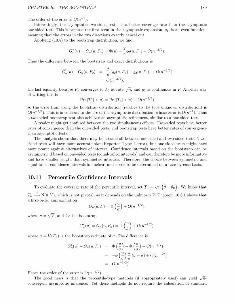
CHAPTER 10. THE BOOTSTRAP 189
The order of the error is O(n−1).Interestingly, the asymptotic two-sided test has a better coverage rate than the asymptotic
one-sided test. This is because the first term in the asymptotic expansion, g1, is an even function,meaning that the errors in the two directions exactly cancel out.
Applying (10.5) to the bootstrap distribution, we find
G∗n(u) = Gn(u, Fn) = Φ(u) +
2
ng2(u, Fn) +O(n−3/2).
Thus the difference between the bootstrap and exact distributions is
G∗n(u)−Gn(u, F0) =
2
n(g2(u, Fn)− g2(u, F0)) +O(n−3/2)
= O(n−3/2),
the last equality because Fn converges to F0 at rate√n, and g2 is continuous in F. Another way
of writing this isPr (|T ∗n | < u) = Pr (|Tn| < u) +O(n−3/2)
so the error from using the bootstrap distribution (relative to the true unknown distribution) isO(n−3/2). This is in contrast to the use of the asymptotic distribution, whose error is O(n−1). Thusa two-sided bootstrap test also achieves an asymptotic refinement, similar to a one-sided test.
A reader might get confused between the two simultaneous effects. Two-sided tests have betterrates of convergence than the one-sided tests, and bootstrap tests have better rates of convergencethan asymptotic tests.
The analysis shows that there may be a trade-off between one-sided and two-sided tests. Two-sided tests will have more accurate size (Reported Type I error), but one-sided tests might havemore power against alternatives of interest. Confidence intervals based on the bootstrap can beasymmetric if based on one-sided tests (equal-tailed intervals) and can therefore be more informativeand have smaller length than symmetric intervals. Therefore, the choice between symmetric andequal-tailed confidence intervals is unclear, and needs to be determined on a case-by-case basis.
10.11 Percentile Confidence Intervals
To evaluate the coverage rate of the percentile interval, set Tn =√n(θ − θ0
). We know that
Tnd−→ N(0, V ), which is not pivotal, as it depends on the unknown V. Theorem 10.8.1 shows that
a first-order approximation
Gn(u, F ) = Φ(uσ
)+O(n−1/2),
where σ =√V , and for the bootstrap
G∗n(u) = Gn(u, Fn) = Φ(uσ
)+O(n−1/2),
where σ = V (Fn) is the bootstrap estimate of σ. The difference is
G∗n(u)−Gn(u, F0) = Φ(uσ
)− Φ
(uσ
)+O(n−1/2)
= −φ(uσ
) uσ
(σ − σ) +O(n−1/2)
= O(n−1/2)
Hence the order of the error is O(n−1/2).The good news is that the percentile-type methods (if appropriately used) can yield
√n-
convergent asymptotic inference. Yet these methods do not require the calculation of standard
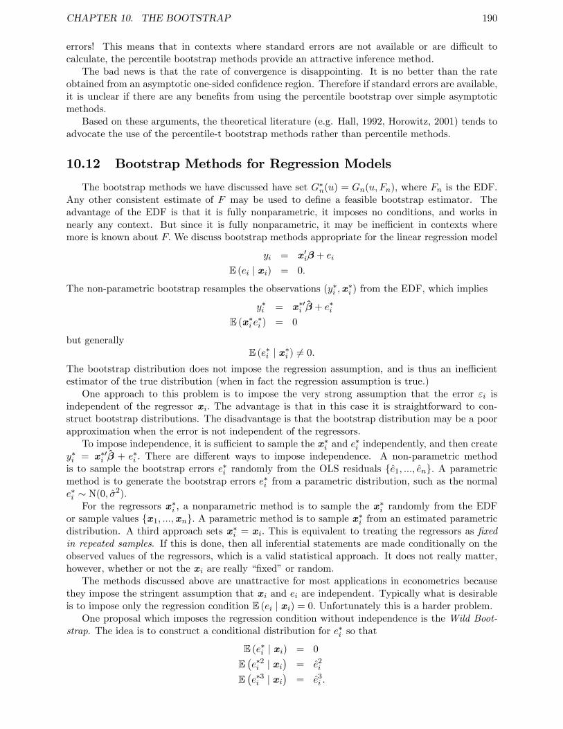
CHAPTER 10. THE BOOTSTRAP 190
errors! This means that in contexts where standard errors are not available or are diffi cult tocalculate, the percentile bootstrap methods provide an attractive inference method.
The bad news is that the rate of convergence is disappointing. It is no better than the rateobtained from an asymptotic one-sided confidence region. Therefore if standard errors are available,it is unclear if there are any benefits from using the percentile bootstrap over simple asymptoticmethods.
Based on these arguments, the theoretical literature (e.g. Hall, 1992, Horowitz, 2001) tends toadvocate the use of the percentile-t bootstrap methods rather than percentile methods.
10.12 Bootstrap Methods for Regression Models
The bootstrap methods we have discussed have set G∗n(u) = Gn(u, Fn), where Fn is the EDF.Any other consistent estimate of F may be used to define a feasible bootstrap estimator. Theadvantage of the EDF is that it is fully nonparametric, it imposes no conditions, and works innearly any context. But since it is fully nonparametric, it may be ineffi cient in contexts wheremore is known about F. We discuss bootstrap methods appropriate for the linear regression model
yi = x′iβ + ei
E (ei | xi) = 0.
The non-parametric bootstrap resamples the observations (y∗i ,x∗i ) from the EDF, which implies
y∗i = x∗′i β + e∗iE (x∗i e
∗i ) = 0
but generallyE (e∗i | x∗i ) 6= 0.
The bootstrap distribution does not impose the regression assumption, and is thus an ineffi cientestimator of the true distribution (when in fact the regression assumption is true.)
One approach to this problem is to impose the very strong assumption that the error εi isindependent of the regressor xi. The advantage is that in this case it is straightforward to con-struct bootstrap distributions. The disadvantage is that the bootstrap distribution may be a poorapproximation when the error is not independent of the regressors.
To impose independence, it is suffi cient to sample the x∗i and e∗i independently, and then create
y∗i = x∗′i β + e∗i . There are different ways to impose independence. A non-parametric methodis to sample the bootstrap errors e∗i randomly from the OLS residuals e1, ..., en. A parametricmethod is to generate the bootstrap errors e∗i from a parametric distribution, such as the normale∗i ∼ N(0, σ2).
For the regressors x∗i , a nonparametric method is to sample the x∗i randomly from the EDF
or sample values x1, ...,xn. A parametric method is to sample x∗i from an estimated parametricdistribution. A third approach sets x∗i = xi. This is equivalent to treating the regressors as fixedin repeated samples. If this is done, then all inferential statements are made conditionally on theobserved values of the regressors, which is a valid statistical approach. It does not really matter,however, whether or not the xi are really “fixed”or random.
The methods discussed above are unattractive for most applications in econometrics becausethey impose the stringent assumption that xi and ei are independent. Typically what is desirableis to impose only the regression condition E (ei | xi) = 0. Unfortunately this is a harder problem.
One proposal which imposes the regression condition without independence is the Wild Boot-strap. The idea is to construct a conditional distribution for e∗i so that
E (e∗i | xi) = 0
E(e∗2i | xi
)= e2
i
E(e∗3i | xi
)= e3
i .
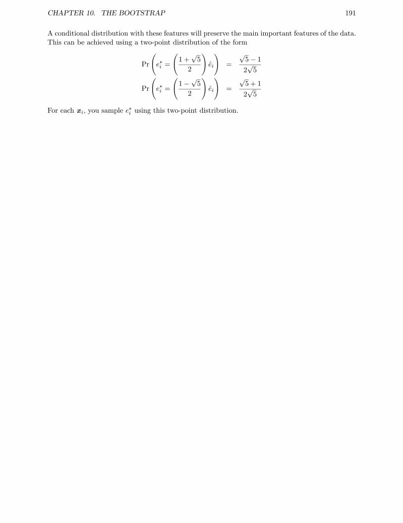
CHAPTER 10. THE BOOTSTRAP 191
A conditional distribution with these features will preserve the main important features of the data.This can be achieved using a two-point distribution of the form
Pr
(e∗i =
(1 +√
5
2
)ei
)=
√5− 1
2√
5
Pr
(e∗i =
(1−√
5
2
)ei
)=
√5 + 1
2√
5
For each xi, you sample e∗i using this two-point distribution.
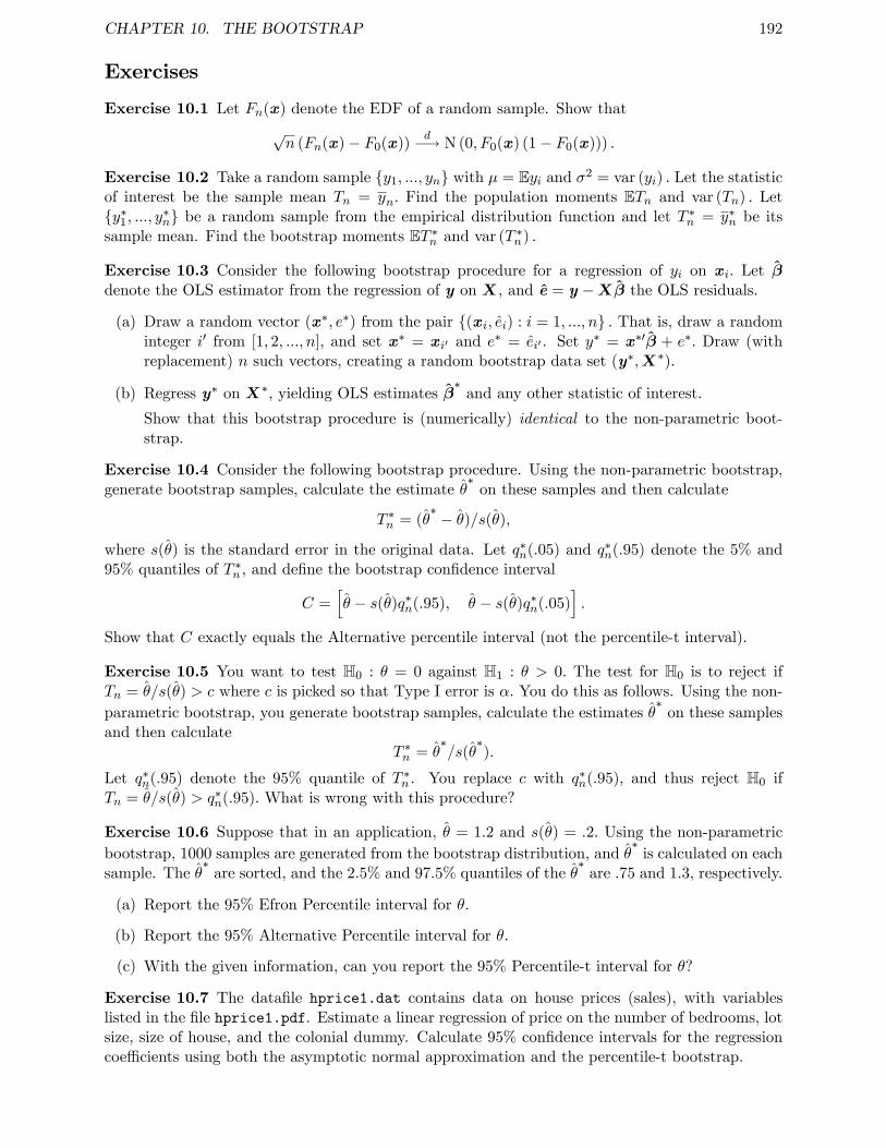
CHAPTER 10. THE BOOTSTRAP 192
Exercises
Exercise 10.1 Let Fn(x) denote the EDF of a random sample. Show that√n (Fn(x)− F0(x))
d−→ N (0, F0(x) (1− F0(x))) .
Exercise 10.2 Take a random sample y1, ..., yn with µ = Eyi and σ2 = var (yi) . Let the statisticof interest be the sample mean Tn = yn. Find the population moments ETn and var (Tn) . Lety∗1, ..., y∗n be a random sample from the empirical distribution function and let T ∗n = y∗n be itssample mean. Find the bootstrap moments ET ∗n and var (T ∗n) .
Exercise 10.3 Consider the following bootstrap procedure for a regression of yi on xi. Let βdenote the OLS estimator from the regression of y on X, and e = y −Xβ the OLS residuals.
(a) Draw a random vector (x∗, e∗) from the pair (xi, ei) : i = 1, ..., n . That is, draw a randominteger i′ from [1, 2, ..., n], and set x∗ = xi′ and e∗ = ei′ . Set y∗ = x∗′β + e∗. Draw (withreplacement) n such vectors, creating a random bootstrap data set (y∗,X∗).
(b) Regress y∗ on X∗, yielding OLS estimates β∗and any other statistic of interest.
Show that this bootstrap procedure is (numerically) identical to the non-parametric boot-strap.
Exercise 10.4 Consider the following bootstrap procedure. Using the non-parametric bootstrap,generate bootstrap samples, calculate the estimate θ
∗on these samples and then calculate
T ∗n = (θ∗ − θ)/s(θ),
where s(θ) is the standard error in the original data. Let q∗n(.05) and q∗n(.95) denote the 5% and95% quantiles of T ∗n , and define the bootstrap confidence interval
C =[θ − s(θ)q∗n(.95), θ − s(θ)q∗n(.05)
].
Show that C exactly equals the Alternative percentile interval (not the percentile-t interval).
Exercise 10.5 You want to test H0 : θ = 0 against H1 : θ > 0. The test for H0 is to reject ifTn = θ/s(θ) > c where c is picked so that Type I error is α. You do this as follows. Using the non-parametric bootstrap, you generate bootstrap samples, calculate the estimates θ
∗on these samples
and then calculateT ∗n = θ
∗/s(θ
∗).
Let q∗n(.95) denote the 95% quantile of T ∗n . You replace c with q∗n(.95), and thus reject H0 ifTn = θ/s(θ) > q∗n(.95). What is wrong with this procedure?
Exercise 10.6 Suppose that in an application, θ = 1.2 and s(θ) = .2. Using the non-parametricbootstrap, 1000 samples are generated from the bootstrap distribution, and θ
∗is calculated on each
sample. The θ∗are sorted, and the 2.5% and 97.5% quantiles of the θ
∗are .75 and 1.3, respectively.
(a) Report the 95% Efron Percentile interval for θ.
(b) Report the 95% Alternative Percentile interval for θ.
(c) With the given information, can you report the 95% Percentile-t interval for θ?
Exercise 10.7 The datafile hprice1.dat contains data on house prices (sales), with variableslisted in the file hprice1.pdf. Estimate a linear regression of price on the number of bedrooms, lotsize, size of house, and the colonial dummy. Calculate 95% confidence intervals for the regressioncoeffi cients using both the asymptotic normal approximation and the percentile-t bootstrap.
Chapter 11
Generalized Method of Moments
11.1 Overidentified Linear Model
Consider the linear model
yi = x′iβ + ei
= x′1iβ1 + x′2iβ2 + ei
E (xiei) = 0
where x1i is k × 1 and x2 is r × 1 with ` = k + r. We know that without further restrictions, anasymptotically effi cient estimator of β is the OLS estimator. Now suppose that we are given theinformation that β2 = 0. Now we can write the model as
yi = x′1iβ1 + ei
E (xiei) = 0.
In this case, how should β1 be estimated? One method is OLS regression of yi on x1i alone. Thismethod, however, is not necessarily effi cient, as there are ` restrictions in E (xiei) = 0, while β1 isof dimension k < `. This situation is called overidentified. There are ` − k = r more momentrestrictions than free parameters. We call r the number of overidentifying restrictions.
This is a special case of a more general class of moment condition models. Let g(y,x, z,β) bean `× 1 function of a k × 1 parameter β with ` ≥ k such that
Eg(yi,xi, zi,β0) = 0 (11.1)
where β0 is the true value of β. In our previous example, g(y,z,β) = z·(y−x′1β). In econometrics,this class of models are called moment condition models. In the statistics literature, these areknown as estimating equations.
As an important special case we will devote special attention to linear moment condition models,which can be written as
yi = x′iβ + ei
E (ziei) = 0.
where the dimensions of xi and zi are k × 1 and ` × 1 , with ` ≥ k. If k = ` the model is justidentified, otherwise it is overidentified. The variables xi may be components and functions ofzi, but this is not required. This model falls in the class (11.1) by setting
g(y,x, z,β0) = z·(y − x′β) (11.2)
193
CHAPTER 11. GENERALIZED METHOD OF MOMENTS 194
11.2 GMM Estimator
Define the sample analog of (11.2)
gn(β) =1
n
n∑i=1
gi(β) =1
n
n∑i=1
zi(yi − x′iβ
)=
1
n
(Z ′y −Z ′Xβ
). (11.3)
The method of moments estimator for β is defined as the parameter value which sets gn(β) = 0.This is generally not possible when ` > k, as there are more equations than free parameters. Theidea of the generalized method of moments (GMM) is to define an estimator which sets gn(β)“close”to zero.
For some `× ` weight matrix W n > 0, let
Jn(β) = n · gn(β)′W n gn(β).
This is a non-negative measure of the “length”of the vector gn(β). For example, ifW n = I, then,Jn(β) = n · gn(β)′gn(β) = n · ‖gn(β)‖2 , the square of the Euclidean length. The GMM estimatorminimizes Jn (β).
Definition 11.2.1 βGMM = argminβ
Jn (β) .
Note that if k = `, then gn(β) = 0, and the GMM estimator is the method of momentsestimator. The first order conditions for the GMM estimator are
0 =∂
∂βJn(β)
= 2∂
∂βgn(β)′W ngn(β)
= −2
(1
nX ′Z
)W n
(1
nZ ′(y −Xβ
))so
2(X ′Z
)W n
(Z ′X
)β = 2
(X ′Z
)W n
(Z ′y
)which establishes the following.
Proposition 11.2.1
βGMM =((X ′Z
)W n
(Z ′X
))−1 (X ′Z
)W n
(Z ′y
).
While the estimator depends onW n, the dependence is only up to scale, for ifW n is replacedby cW n for some c > 0, βGMM does not change.
CHAPTER 11. GENERALIZED METHOD OF MOMENTS 195
11.3 Distribution of GMM Estimator
Assume that W np−→W > 0. Let
Q = E(zix
′i
)and
Ω = E(ziz′ie
2i
)= E
(gig′i
),
where gi = ziei. Then (1
nX ′Z
)W n
(1
nZ ′X
)p−→ Q′WQ
and (1
nX ′Z
)W n
(1√nZ ′e
)d−→ Q′WN (0,Ω) .
We conclude:
Theorem 11.3.1 Asymptotic Distribution of GMM Estimator
√n(β − β
)d−→ N (0,V β) ,
whereV β =
(Q′WQ
)−1 (Q′WΩWQ
) (Q′WQ
)−1.
In general, GMM estimators are asymptotically normal with “sandwich form”asymptotic vari-ances.
The optimal weight matrix W 0 is one which minimizes V β. This turns out to be W 0 = Ω−1.The proof is left as an exercise. This yields the effi cient GMM estimator:
β =(X ′ZΩ−1Z ′X
)−1X ′ZΩ−1Z ′y.
Thus we have
Theorem 11.3.2 Asymptotic Distribution of Effi cient GMM Es-timator √
n(β − β
)d−→ N
(0,(Q′Ω−1Q
)−1).
W 0 = Ω−1 is not known in practice, but it can be estimated consistently. For anyW np−→W 0,
we still call β the effi cient GMM estimator, as it has the same asymptotic distribution.By “effi cient”, we mean that this estimator has the smallest asymptotic variance in the class
of GMM estimators with this set of moment conditions. This is a weak concept of optimality, aswe are only considering alternative weight matrices W n. However, it turns out that the GMMestimator is semiparametrically effi cient, as shown by Gary Chamberlain (1987).
If it is known that E (gi(β)) = 0, and this is all that is known, this is a semi-parametricproblem, as the distribution of the data is unknown. Chamberlain showed that in this context,no semiparametric estimator (one which is consistent globally for the class of models considered)can have a smaller asymptotic variance than
(G′Ω−1G
)−1where G = E ∂
∂β′gi(β). Since the GMM
estimator has this asymptotic variance, it is semiparametrically effi cient.This result shows that in the linear model, no estimator has greater asymptotic effi ciency than
the effi cient linear GMM estimator. No estimator can do better (in this first-order asymptoticsense), without imposing additional assumptions.
CHAPTER 11. GENERALIZED METHOD OF MOMENTS 196
11.4 Estimation of the Effi cient Weight Matrix
Given any weight matrix W n > 0, the GMM estimator β is consistent yet ineffi cient. Forexample, we can set W n = I`. In the linear model, a better choice is W n = (Z ′Z)
−1. Given
any such first-step estimator, we can define the residuals ei = yi − x′iβ and moment equationsgi = ziei = g(yi,xi, zi, β). Construct
gn = gn(β) =1
n
n∑i=1
gi,
g∗i = gi − gn,and define
W n =
(1
n
n∑i=1
g∗i g∗′i
)−1
=
(1
n
n∑i=1
gig′i − gng′n
)−1
. (11.4)
Then W np−→ Ω−1 = W 0, and GMM using W n as the weight matrix is asymptotically effi cient.
A common alternative choice is to set
W n =
(1
n
n∑i=1
gig′i
)−1
which uses the uncentered moment conditions. Since Egi = 0, these two estimators are asymptot-ically equivalent under the hypothesis of correct specification. However, Alastair Hall (2000) hasshown that the uncentered estimator is a poor choice. When constructing hypothesis tests, underthe alternative hypothesis the moment conditions are violated, i.e. Egi 6= 0, so the uncenteredestimator will contain an undesirable bias term and the power of the test will be adversely affected.A simple solution is to use the centered moment conditions to construct the weight matrix, as in(11.4) above.
Here is a simple way to compute the effi cient GMM estimator for the linear model. First, setW n = (Z ′Z)−1, estimate β using this weight matrix, and construct the residual ei = yi − x′iβ.Then set gi = ziei, and let g be the associated n× ` matrix. Then the effi cient GMM estimator is
β =(X ′Z
(g′g − ngng′n
)−1Z ′X
)−1X ′Z
(g′g − ngng′n
)−1Z ′y.
In most cases, when we say “GMM”, we actually mean “effi cient GMM”. There is little point inusing an ineffi cient GMM estimator when the effi cient estimator is easy to compute.
An estimator of the asymptotic variance of β can be seen from the above formula. Set
V = n(X ′Z
(g′g − ngng′n
)−1Z ′X
)−1.
Asymptotic standard errors are given by the square roots of the diagonal elements of V .There is an important alternative to the two-step GMM estimator just described. Instead, we
can let the weight matrix be considered as a function of β. The criterion function is then
J(β) = n · gn(β)′
(1
n
n∑i=1
g∗i (β)g∗i (β)′
)−1
gn(β).
whereg∗i (β) = gi(β)− gn(β)
The β which minimizes this function is called the continuously-updated GMM estimator, andwas introduced by L. Hansen, Heaton and Yaron (1996).
The estimator appears to have some better properties than traditional GMM, but can be nu-merically tricky to obtain in some cases. This is a current area of research in econometrics.
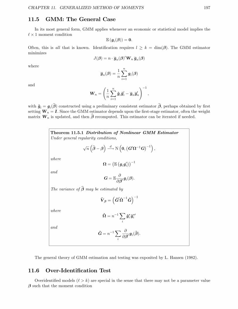
CHAPTER 11. GENERALIZED METHOD OF MOMENTS 197
11.5 GMM: The General Case
In its most general form, GMM applies whenever an economic or statistical model implies the`× 1 moment condition
E (gi(β)) = 0.
Often, this is all that is known. Identification requires l ≥ k = dim(β). The GMM estimatorminimizes
J(β) = n · gn(β)′W n gn(β)
where
gn(β) =1
n
n∑i=1
gi(β)
and
W n =
(1
n
n∑i=1
gig′i − gng′n
)−1
,
with gi = gi(β) constructed using a preliminary consistent estimator β, perhaps obtained by firstsettingW n = I. Since the GMM estimator depends upon the first-stage estimator, often the weightmatrix W n is updated, and then β recomputed. This estimator can be iterated if needed.
Theorem 11.5.1 Distribution of Nonlinear GMM EstimatorUnder general regularity conditions,
√n(β − β
)d−→ N
(0,(G′Ω−1G
)−1),
whereΩ =
(E(gig′i
))−1
and
G = E∂
∂β′gi(β).
The variance of β may be estimated by
V β =(G′Ω−1G)−1
whereΩ = n−1
∑i
g∗i g∗′i
and
G = n−1∑i
∂
∂β′gi(β).
The general theory of GMM estimation and testing was exposited by L. Hansen (1982).
11.6 Over-Identification Test
Overidentified models (` > k) are special in the sense that there may not be a parameter valueβ such that the moment condition
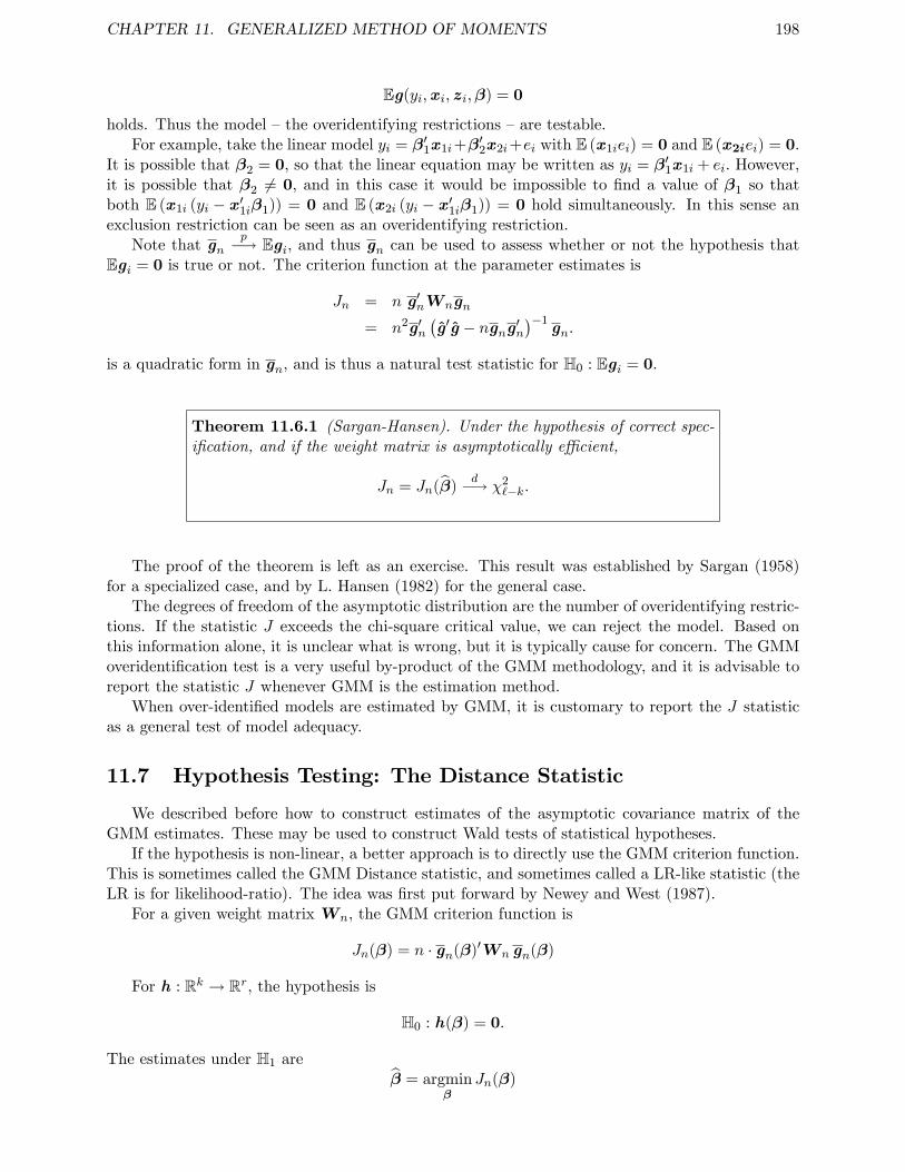
CHAPTER 11. GENERALIZED METHOD OF MOMENTS 198
Eg(yi,xi, zi,β) = 0
holds. Thus the model —the overidentifying restrictions —are testable.For example, take the linear model yi = β′1x1i+β
′2x2i+ei with E (x1iei) = 0 and E (x2iei) = 0.
It is possible that β2 = 0, so that the linear equation may be written as yi = β′1x1i + ei. However,it is possible that β2 6= 0, and in this case it would be impossible to find a value of β1 so thatboth E (x1i (yi − x′1iβ1)) = 0 and E (x2i (yi − x′1iβ1)) = 0 hold simultaneously. In this sense anexclusion restriction can be seen as an overidentifying restriction.
Note that gnp−→ Egi, and thus gn can be used to assess whether or not the hypothesis that
Egi = 0 is true or not. The criterion function at the parameter estimates is
Jn = n g′nW ngn
= n2g′n(g′g − ngng′n
)−1gn.
is a quadratic form in gn, and is thus a natural test statistic for H0 : Egi = 0.
Theorem 11.6.1 (Sargan-Hansen). Under the hypothesis of correct spec-ification, and if the weight matrix is asymptotically effi cient,
Jn = Jn(β)d−→ χ2
`−k.
The proof of the theorem is left as an exercise. This result was established by Sargan (1958)for a specialized case, and by L. Hansen (1982) for the general case.
The degrees of freedom of the asymptotic distribution are the number of overidentifying restric-tions. If the statistic J exceeds the chi-square critical value, we can reject the model. Based onthis information alone, it is unclear what is wrong, but it is typically cause for concern. The GMMoveridentification test is a very useful by-product of the GMM methodology, and it is advisable toreport the statistic J whenever GMM is the estimation method.
When over-identified models are estimated by GMM, it is customary to report the J statisticas a general test of model adequacy.
11.7 Hypothesis Testing: The Distance Statistic
We described before how to construct estimates of the asymptotic covariance matrix of theGMM estimates. These may be used to construct Wald tests of statistical hypotheses.
If the hypothesis is non-linear, a better approach is to directly use the GMM criterion function.This is sometimes called the GMM Distance statistic, and sometimes called a LR-like statistic (theLR is for likelihood-ratio). The idea was first put forward by Newey and West (1987).
For a given weight matrix W n, the GMM criterion function is
Jn(β) = n · gn(β)′W n gn(β)
For h : Rk → Rr, the hypothesis is
H0 : h(β) = 0.
The estimates under H1 areβ = argmin
βJn(β)
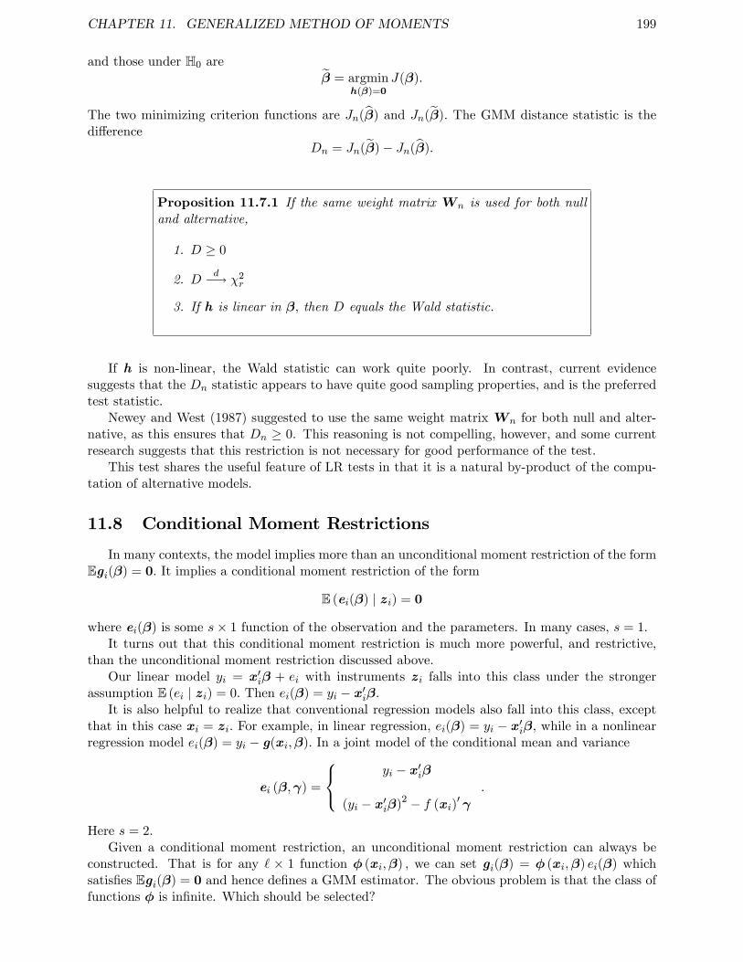
CHAPTER 11. GENERALIZED METHOD OF MOMENTS 199
and those under H0 areβ = argmin
h(β)=0J(β).
The two minimizing criterion functions are Jn(β) and Jn(β). The GMM distance statistic is thedifference
Dn = Jn(β)− Jn(β).
Proposition 11.7.1 If the same weight matrix W n is used for both nulland alternative,
1. D ≥ 0
2. D d−→ χ2r
3. If h is linear in β, then D equals the Wald statistic.
If h is non-linear, the Wald statistic can work quite poorly. In contrast, current evidencesuggests that the Dn statistic appears to have quite good sampling properties, and is the preferredtest statistic.
Newey and West (1987) suggested to use the same weight matrix W n for both null and alter-native, as this ensures that Dn ≥ 0. This reasoning is not compelling, however, and some currentresearch suggests that this restriction is not necessary for good performance of the test.
This test shares the useful feature of LR tests in that it is a natural by-product of the compu-tation of alternative models.
11.8 Conditional Moment Restrictions
In many contexts, the model implies more than an unconditional moment restriction of the formEgi(β) = 0. It implies a conditional moment restriction of the form
E (ei(β) | zi) = 0
where ei(β) is some s× 1 function of the observation and the parameters. In many cases, s = 1.It turns out that this conditional moment restriction is much more powerful, and restrictive,
than the unconditional moment restriction discussed above.Our linear model yi = x′iβ + ei with instruments zi falls into this class under the stronger
assumption E (ei | zi) = 0. Then ei(β) = yi − x′iβ.It is also helpful to realize that conventional regression models also fall into this class, except
that in this case xi = zi. For example, in linear regression, ei(β) = yi − x′iβ, while in a nonlinearregression model ei(β) = yi − g(xi,β). In a joint model of the conditional mean and variance
ei (β,γ) =
yi − x′iβ
(yi − x′iβ)2 − f (xi)′ γ
.
Here s = 2.Given a conditional moment restriction, an unconditional moment restriction can always be
constructed. That is for any ` × 1 function φ (xi,β) , we can set gi(β) = φ (xi,β) ei(β) whichsatisfies Egi(β) = 0 and hence defines a GMM estimator. The obvious problem is that the class offunctions φ is infinite. Which should be selected?
CHAPTER 11. GENERALIZED METHOD OF MOMENTS 200
This is equivalent to the problem of selection of the best instruments. If xi ∈ R is a validinstrument satisfying E (ei | xi) = 0, then xi, x
2i , x
3i , ..., etc., are all valid instruments. Which
should be used?One solution is to construct an infinite list of potent instruments, and then use the first k
instruments. How is k to be determined? This is an area of theory still under development. Arecent study of this problem is Donald and Newey (2001).
Another approach is to construct the optimal instrument. The form was uncovered by Cham-berlain (1987). Take the case s = 1. Let
Ri = E(∂
∂βei(β) | zi
)and
σ2i = E
(ei(β)2 | zi
).
Then the “optimal instrument”isAi = −σ−2
i Ri
so the optimal moment isgi(β) = Aiei(β).
Setting gi (β) to be this choice (which is k×1, so is just-identified) yields the best GMM estimatorpossible.
In practice, Ai is unknown, but its form does help us think about construction of optimalinstruments.
In the linear model ei(β) = yi − x′iβ, note that
Ri = −E (xi | zi)
andσ2i = E
(e2i | zi
),
soAi = σ−2
i E (xi | zi) .
In the case of linear regression, xi = zi, so Ai = σ−2i zi. Hence effi cient GMM is GLS, as we
discussed earlier in the course.In the case of endogenous variables, note that the effi cient instrumentAi involves the estimation
of the conditional mean of xi given zi. In other words, to get the best instrument for xi, we need thebest conditional mean model for xi given zi, not just an arbitrary linear projection. The effi cientinstrument is also inversely proportional to the conditional variance of ei. This is the same as theGLS estimator; namely that improved effi ciency can be obtained if the observations are weightedinversely to the conditional variance of the errors.
11.9 Bootstrap GMM Inference
Let β be the 2SLS or GMM estimator of β. Using the EDF of (yi, zi,xi), we can apply thebootstrap methods discussed in Chapter 10 to compute estimates of the bias and variance of β,and construct confidence intervals for β, identically as in the regression model. However, cautionshould be applied when interpreting such results.
A straightforward application of the nonparametric bootstrap works in the sense of consistentlyachieving the first-order asymptotic distribution. This has been shown by Hahn (1996). However,it fails to achieve an asymptotic refinement when the model is over-identified, jeopardizing thetheoretical justification for percentile-t methods. Furthermore, the bootstrap applied J test willyield the wrong answer.
CHAPTER 11. GENERALIZED METHOD OF MOMENTS 201
The problem is that in the sample, β is the “true”value and yet gn(β) 6= 0. Thus according torandom variables (y∗i , z
∗i ,x∗i ) drawn from the EDF Fn,
E(gi
(β))
= gn(β) 6= 0.
This means that (y∗i , z∗i ,x∗i ) do not satisfy the same moment conditions as the population distrib-
ution.A correction suggested by Hall and Horowitz (1996) can solve the problem. Given the bootstrap
sample (y∗,Z∗,X∗), define the bootstrap GMM criterion
J∗n(β) = n ·(g∗n(β)− gn(β)
)′W ∗
n
(g∗n(β)− gn(β)
)where gn(β) is from the in-sample data, not from the bootstrap data.
Let β∗minimize J∗n(β), and define all statistics and tests accordingly. In the linear model, this
implies that the bootstrap estimator is
β∗n =
(X∗′Z∗W ∗
nZ∗′X∗
)−1 (X∗′Z∗W ∗
n
(Z∗′y∗ −Z ′e
)).
where e = y −Xβ are the in-sample residuals. The bootstrap J statistic is J∗n(β∗).
Brown and Newey (2002) have an alternative solution. They note that we can sample fromthe observations with the empirical likelihood probabilities pi described in Chapter 12. Since∑n
i=1 pigi
(β)
= 0, this sampling scheme preserves the moment conditions of the model, so no
recentering or adjustments is needed. Brown and Newey argue that this bootstrap procedure willbe more effi cient than the Hall-Horowitz GMM bootstrap.
CHAPTER 11. GENERALIZED METHOD OF MOMENTS 202
Exercises
Exercise 11.1 Take the model
yi = x′iβ + ei
E (xiei) = 0
e2i = z′iγ + ηi
E (ziηi) = 0.
Find the method of moments estimators(β, γ
)for (β,γ) .
Exercise 11.2 Take the single equation
y = Xβ + e
E (e | Z) = 0
Assume E(e2i | zi
)= σ2. Show that if β is estimated by GMM with weight matrixW n = (Z ′Z)
−1,
then √n(β − β
)d−→ N
(0, σ2
(Q′M−1Q
)−1)
where Q = E (zix′i) andM = E (ziz
′i) .
Exercise 11.3 Take the model yi = x′iβ + ei with E (ziei) = 0. Let ei = yi − x′iβ where β isconsistent for β (e.g. a GMM estimator with arbitrary weight matrix). Define the estimate of theoptimal GMM weight matrix
W n =
(1
n
n∑i=1
ziz′ie
2i
)−1
.
Show that W np−→ Ω−1 where Ω = E
(ziz′ie
2i
).
Exercise 11.4 In the linear model estimated by GMM with general weight matrixW , the asymp-totic variance of βGMM is
V =(Q′WQ
)−1Q′WΩWQ
(Q′WQ
)−1
(a) Let V 0 be this matrix when W = Ω−1. Show that V 0 =(Q′Ω−1Q
)−1.
(b) We want to show that for anyW , V −V 0 is positive semi-definite (for then V 0 is the smallerpossible covariance matrix andW = Ω−1 is the effi cient weight matrix). To do this, start byfinding matrices A and B such that V = A′ΩA and V 0 = B′ΩB.
(c) Show that B′ΩA = B′ΩB and therefore that B′Ω (A−B) = 0.
(d) Use the expressions V = A′ΩA, A = B + (A−B) , and B′Ω (A−B) = 0 to show thatV ≥ V 0.
Exercise 11.5 The equation of interest is
yi = g(xi,β) + ei
E (ziei) = 0.
The observed data is (yi, zi,xi). zi is `×1 and β is k×1, ` ≥ k. Show how to construct an effi cientGMM estimator for β.
CHAPTER 11. GENERALIZED METHOD OF MOMENTS 203
Exercise 11.6 In the linear model y = Xβ + e with E(xiei) = 0, a Generalized Method ofMoments (GMM) criterion function for β is defined as
Jn(β) =1
n(y −Xβ)′XΩ
−1X ′ (y −Xβ) (11.5)
where Ω = 1n
∑ni=1 xix
′ie
2i , ei = yi−x′iβ are the OLS residuals, and β = (X ′X)
−1X ′Y is LS. The
GMM estimator of β, subject to the restriction h(β) = 0, is defined as
β = argminh(β)=0
Jn(β).
The GMM test statistic (the distance statistic) of the hypothesis h(β) = 0 is
D = Jn(β) = minh(β)=0
Jn(β). (11.6)
(a) Show that you can rewrite Jn(β) in (11.5) as
Jn(β) = n(β − β
)′V−1β
(β − β
)thus β is the same as the minimum distance estimator.
(b) Show that in this setting, the distance statistic D in (11.6) equals the Wald statistic.
Exercise 11.7 Take the linear model
yi = x′iβ + ei
E (ziei) = 0.
and consider the GMM estimator β of β. Let
Jn = ngn(β)′Ω−1gn(β)
denote the test of overidentifying restrictions. Show that Jnd−→ χ2
`−k as n→∞ by demonstratingeach of the following:
(a) Since Ω > 0, we can write Ω−1 = CC ′ and Ω = C ′−1C−1
(b) Jn = n(C ′gn(β)
)′ (C ′ΩC
)−1C ′gn(β)
(c) C ′gn(β) = DnC′gn(β0) where
Dn = I` −C ′(
1
nZ ′X
)((1
nX ′Z
)Ω−1(
1
nZ ′X
))−1( 1
nX ′Z
)Ω−1C ′−1
gn(β0) =1
nZ ′e.
(d) Dnp−→ I` −R (R′R)
−1R′ where R = C ′E (zix
′i)
(e) n1/2C ′gn(β0)d−→X ∼ N (0, I`)
(f) Jnd−→X ′
(I` −R (R′R)
−1R′)X
(g) X ′(I` −R (R′R)
−1R′)X ∼ χ2
`−k.
Hint: I` −R (R′R)−1R′ is a projection matrix.
Chapter 12
Empirical Likelihood
12.1 Non-Parametric Likelihood
An alternative to GMM is empirical likelihood. The idea is due to Art Owen (1988, 2001) andhas been extended to moment condition models by Qin and Lawless (1994). It is a non-parametricanalog of likelihood estimation.
The idea is to construct a multinomial distribution F (p1, ..., pn) which places probability piat each observation. To be a valid multinomial distribution, these probabilities must satisfy therequirements that pi ≥ 0 and
n∑i=1
pi = 1. (12.1)
Since each observation is observed once in the sample, the log-likelihood function for this multino-mial distribution is
logL (p1, ..., pn) =
n∑i=1
log(pi). (12.2)
First let us consider a just-identified model. In this case the moment condition places noadditional restrictions on the multinomial distribution. The maximum likelihood estimators ofthe probabilities (p1, ..., pn) are those which maximize the log-likelihood subject to the constraint(12.1). This is equivalent to maximizing
n∑i=1
log(pi)− µ(
n∑i=1
pi − 1
)
where µ is a Lagrange multiplier. The n first order conditions are 0 = p−1i −µ. Combined with the
constraint (12.1) we find that the MLE is pi = n−1 yielding the log-likelihood −n log(n).Now consider the case of an overidentified model with moment condition
Egi(β0) = 0
where g is `× 1 and β is k× 1 and for simplicity we write gi(β) = g(yi, zi,xi,β). The multinomialdistribution which places probability pi at each observation (yi,xi, zi) will satisfy this condition ifand only if
n∑i=1
pigi(β) = 0 (12.3)
The empirical likelihood estimator is the value of β which maximizes the multinomial log-likelihood (12.2) subject to the restrictions (12.1) and (12.3).
204
CHAPTER 12. EMPIRICAL LIKELIHOOD 205
The Lagrangian for this maximization problem is
L (β, p1, ..., pn,λ, µ) =
n∑i=1
log(pi)− µ(
n∑i=1
pi − 1
)− nλ′
n∑i=1
pigi (β)
where λ and µ are Lagrange multipliers. The first-order-conditions of L with respect to pi, µ, andλ are
1
pi= µ+ nλ′gi (β)
n∑i=1
pi = 1
n∑i=1
pigi (β) = 0.
Multiplying the first equation by pi, summing over i, and using the second and third equations, wefind µ = n and
pi =1
n(1 + λ′gi (β)
) .Substituting into L we find
R (β,λ) = −n log (n)−n∑i=1
log(1 + λ′gi (β)
). (12.4)
For given β, the Lagrange multiplier λ(β) minimizes R (β,λ) :
λ(β) = argminλ
R(β,λ). (12.5)
This minimization problem is the dual of the constrained maximization problem. The solution(when it exists) is well defined since R(β,λ) is a convex function of λ. The solution cannot beobtained explicitly, but must be obtained numerically (see section 6.5). This yields the (profile)empirical log-likelihood function for β.
R(β) = R(β,λ(β))
= −n log (n)−n∑i=1
log(1 + λ(β)′gi (β)
)The EL estimate β is the value which maximizes R(β), or equivalently minimizes its negative
β = argminβ
[−R(β)] (12.6)
Numerical methods are required for calculation of β (see Section 12.5).As a by-product of estimation, we also obtain the Lagrange multiplier λ = λ(β), probabilities
pi =1
n(
1 + λ′gi
(β)) .
and maximized empirical likelihood
R(β) =n∑i=1
log (pi) . (12.7)
CHAPTER 12. EMPIRICAL LIKELIHOOD 206
12.2 Asymptotic Distribution of EL Estimator
Define
Gi (β) =∂
∂β′gi (β) (12.8)
G = EGi (β0)
Ω = E(gi (β0) gi (β0)′
)and
V =(G′Ω−1G
)−1(12.9)
V λ = Ω−G(G′Ω−1G
)−1G′ (12.10)
For example, in the linear model, Gi (β) = −zix′i, G = −E (zix′i), and Ω = E
(ziz′ie
2i
).
Theorem 12.2.1 Under regularity conditions,
√n(β − β0
)d−→ N (0,V β)
√nλ
d−→ Ω−1N (0,V λ)
where V and V λ are defined in (12.9) and (12.10), and√n(β − β0
)and
√nλ are asymptotically independent.
The theorem shows that asymptotic variance V β for β is the same as for effi cient GMM. Thusthe EL estimator is asymptotically effi cient.
Chamberlain (1987) showed that V β is the semiparametric effi ciency bound for β in the overi-dentified moment condition model. This means that no consistent estimator for this class of modelscan have a lower asymptotic variance than V β. Since the EL estimator achieves this bound, it isan asymptotically effi cient estimator for β.
Proof of Theorem 12.2.1. (β, λ) jointly solve
0 =∂
∂λR(β,λ) = −
n∑i=1
gi
(β)
(1 + λ
′gi
(β)) (12.11)
0 =∂
∂βR(β,λ) = −
n∑i=1
Gi
(β)′λ
1 + λ′gi
(β) . (12.12)
Let Gn = 1n
∑ni=1Gi (β0) , gn = 1
n
∑ni=1 gi (β0) and Ωn = 1
n
∑ni=1 gi (β0) gi (β0)′ .
Expanding (12.12) around β = β0 and λ = λ0 = 0 yields
0 ' G′n(λ− λ0
). (12.13)
Expanding (12.11) around β = β0 and λ = λ0 = 0 yields
0 ' −gn −Gn
(β − β0
)+ Ωnλ (12.14)
CHAPTER 12. EMPIRICAL LIKELIHOOD 207
Premultiplying by G′nΩ−1n and using (12.13) yields
0 ' −G′nΩ−1n gn −G′nΩ−1
n Gn
(β − β0
)+G′nΩ
−1n Ωnλ
= −G′nΩ−1n gn −G′nΩ−1
n Gn
(β − β0
)Solving for β and using the WLLN and CLT yields
√n(β − β0
)' −
(G′nΩ
−1n Gn
)−1G′nΩ
−1n
√ngn (12.15)
d−→(G′Ω−1G
)−1G′Ω−1N (0,Ω)
= N (0,V β)
Solving (12.14) for λ and using (12.15) yields
√nλ ' Ω−1
n
(I −Gn
(G′nΩ
−1n Gn
)−1G′nΩ
−1n
)√ngn (12.16)
d−→ Ω−1(I −G
(G′Ω−1G
)−1G′Ω−1
)N (0,Ω)
= Ω−1N (0,V λ)
Furthermore, since
G′(I −Ω−1G
(G′Ω−1G
)−1G′)
= 0
√n(β − β0
)and√nλ are asymptotically uncorrelated and hence independent.
12.3 Overidentifying Restrictions
In a parametric likelihood context, tests are based on the difference in the log likelihood func-tions. The same statistic can be constructed for empirical likelihood. Twice the difference betweenthe unrestricted empirical log-likelihood −n log (n) and the maximized empirical log-likelihood forthe model (12.7) is
LRn =n∑i=1
2 log(
1 + λ′gi
(β))
. (12.17)
Theorem 12.3.1 If Egi(β0) = 0 then LRnd−→ χ2
`−k.
The EL overidentification test is similar to the GMM overidentification test. They are asymp-totically first-order equivalent, and have the same interpretation. The overidentification test is avery useful by-product of EL estimation, and it is advisable to report the statistic LRn wheneverEL is the estimation method.
Proof of Theorem 12.3.1. First, by a Taylor expansion, (12.15), and (12.16),
1√n
n∑i=1
gi
(β)'√n(gn +Gn
(β − β0
))'
(I −Gn
(G′nΩ
−1n Gn
)−1G′nΩ
−1n
)√ngn
' Ωn
√nλ.
CHAPTER 12. EMPIRICAL LIKELIHOOD 208
Second, since log(1 + u) ' u− u2/2 for u small,
LRn =
n∑i=1
2 log(
1 + λ′gi
(β))
' 2λ′n∑i=1
gi
(β)− λ′
n∑i=1
gi
(β)gi
(β)′λ
' nλ′Ωnλ
d−→ N (0,V λ)′Ω−1N (0,V λ)
= χ2`−k
where the proof of the final equality is left as an exercise.
12.4 Testing
Let the maintained model beEgi(β) = 0 (12.18)
where g is ` × 1 and β is k × 1. By “maintained” we mean that the overidentfying restrictionscontained in (12.18) are assumed to hold and are not being challenged (at least for the test discussedin this section). The hypothesis of interest is
h(β) = 0.
where h : Rk → Ra. The restricted EL estimator and likelihood are the values which solve
β = argmaxh(β)=0
R(β)
R(β) = maxh(β)=0
R(β).
Fundamentally, the restricted EL estimator β is simply an EL estimator with `−k+a overidentifyingrestrictions, so there is no fundamental change in the distribution theory for β relative to β. To testthe hypothesis h(β) while maintaining (12.18), the simple overidentifying restrictions test (12.17)is not appropriate. Instead we use the difference in log-likelihoods:
LRn = 2(R(β)−R(β)
).
This test statistic is a natural analog of the GMM distance statistic.
Theorem 12.4.1 Under (12.18) and H0 : h(β) = 0, LRnd−→ χ2
a.
The proof of this result is more challenging and is omitted.
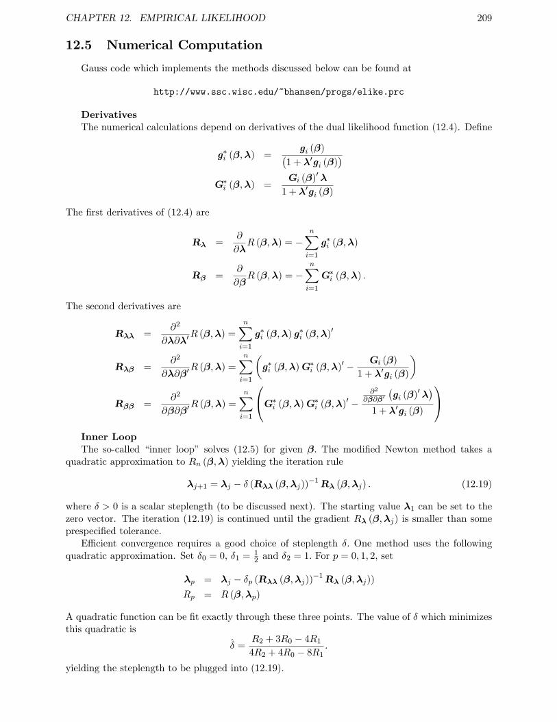
CHAPTER 12. EMPIRICAL LIKELIHOOD 209
12.5 Numerical Computation
Gauss code which implements the methods discussed below can be found at
http://www.ssc.wisc.edu/~bhansen/progs/elike.prc
DerivativesThe numerical calculations depend on derivatives of the dual likelihood function (12.4). Define
g∗i (β,λ) =gi (β)(
1 + λ′gi (β))
G∗i (β,λ) =Gi (β)′ λ
1 + λ′gi (β)
The first derivatives of (12.4) are
Rλ =∂
∂λR (β,λ) = −
n∑i=1
g∗i (β,λ)
Rβ =∂
∂βR (β,λ) = −
n∑i=1
G∗i (β,λ) .
The second derivatives are
Rλλ =∂2
∂λ∂λ′R (β,λ) =
n∑i=1
g∗i (β,λ) g∗i (β,λ)′
Rλβ =∂2
∂λ∂β′R (β,λ) =
n∑i=1
(g∗i (β,λ)G∗i (β,λ)′ − Gi (β)
1 + λ′gi (β)
)
Rββ =∂2
∂β∂β′R (β,λ) =
n∑i=1
G∗i (β,λ)G∗i (β,λ)′ −∂2
∂β∂β′(gi (β)′ λ
)1 + λ′gi (β)
Inner LoopThe so-called “inner loop” solves (12.5) for given β. The modified Newton method takes a
quadratic approximation to Rn (β,λ) yielding the iteration rule
λj+1 = λj − δ (Rλλ (β,λj))−1Rλ (β,λj) . (12.19)
where δ > 0 is a scalar steplength (to be discussed next). The starting value λ1 can be set to thezero vector. The iteration (12.19) is continued until the gradient Rλ (β,λj) is smaller than someprespecified tolerance.
Effi cient convergence requires a good choice of steplength δ. One method uses the followingquadratic approximation. Set δ0 = 0, δ1 = 1
2 and δ2 = 1. For p = 0, 1, 2, set
λp = λj − δp (Rλλ (β,λj))−1Rλ (β,λj))
Rp = R (β,λp)
A quadratic function can be fit exactly through these three points. The value of δ which minimizesthis quadratic is
δ =R2 + 3R0 − 4R1
4R2 + 4R0 − 8R1.
yielding the steplength to be plugged into (12.19).
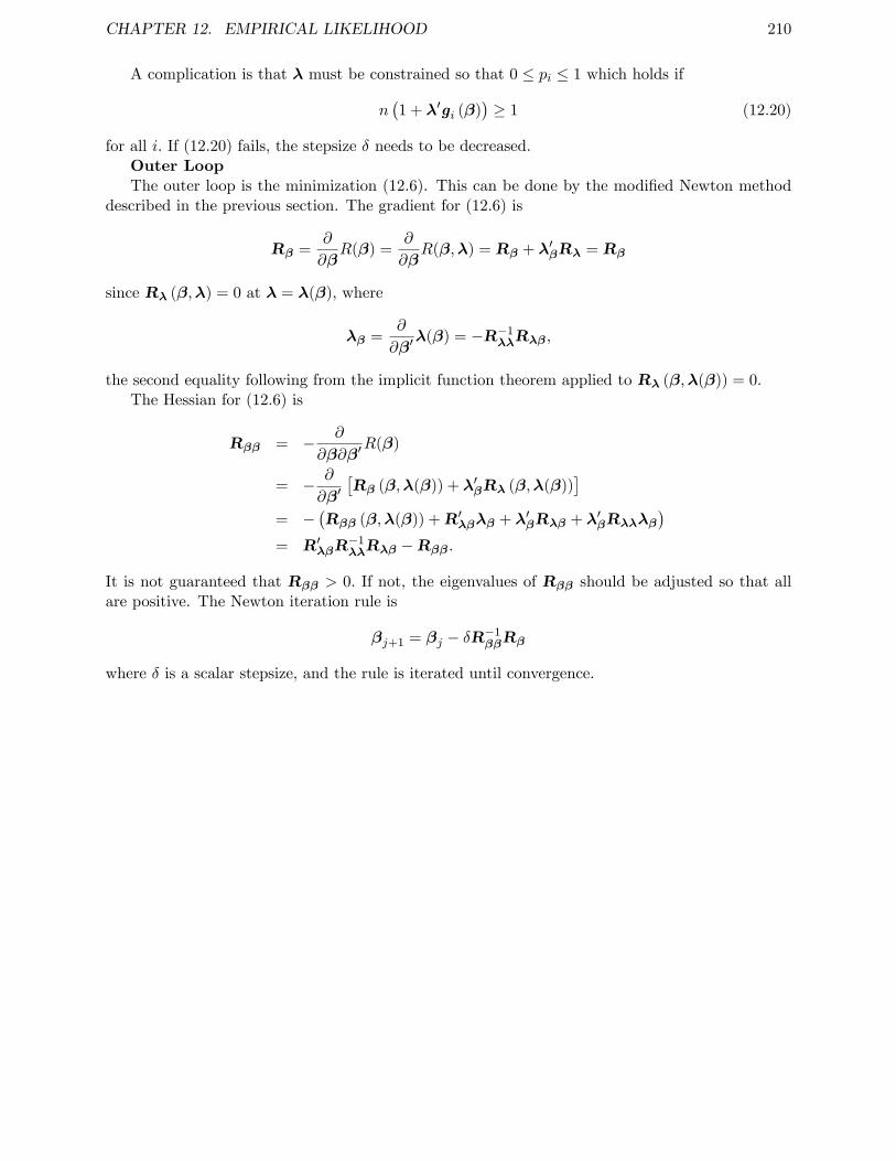
CHAPTER 12. EMPIRICAL LIKELIHOOD 210
A complication is that λ must be constrained so that 0 ≤ pi ≤ 1 which holds if
n(1 + λ′gi (β)
)≥ 1 (12.20)
for all i. If (12.20) fails, the stepsize δ needs to be decreased.Outer LoopThe outer loop is the minimization (12.6). This can be done by the modified Newton method
described in the previous section. The gradient for (12.6) is
Rβ =∂
∂βR(β) =
∂
∂βR(β,λ) = Rβ + λ′βRλ = Rβ
since Rλ (β,λ) = 0 at λ = λ(β), where
λβ =∂
∂β′λ(β) = −R−1
λλRλβ,
the second equality following from the implicit function theorem applied to Rλ (β,λ(β)) = 0.The Hessian for (12.6) is
Rββ = − ∂
∂β∂β′R(β)
= − ∂
∂β′[Rβ (β,λ(β)) + λ′βRλ (β,λ(β))
]= −
(Rββ (β,λ(β)) +R′λβλβ + λ′βRλβ + λ′βRλλλβ
)= R′λβR
−1λλRλβ −Rββ.
It is not guaranteed that Rββ > 0. If not, the eigenvalues of Rββ should be adjusted so that allare positive. The Newton iteration rule is
βj+1 = βj − δR−1ββRβ
where δ is a scalar stepsize, and the rule is iterated until convergence.
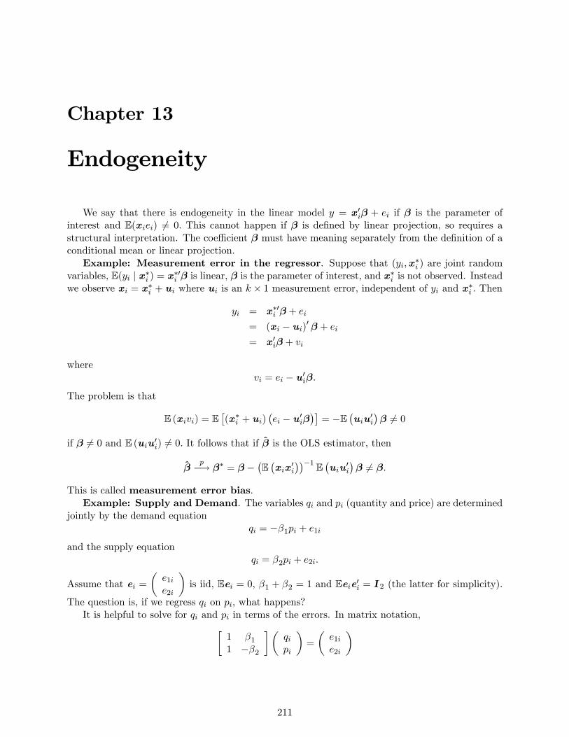
Chapter 13
Endogeneity
We say that there is endogeneity in the linear model y = x′iβ + ei if β is the parameter ofinterest and E(xiei) 6= 0. This cannot happen if β is defined by linear projection, so requires astructural interpretation. The coeffi cient β must have meaning separately from the definition of aconditional mean or linear projection.
Example: Measurement error in the regressor. Suppose that (yi,x∗i ) are joint random
variables, E(yi | x∗i ) = x∗′i β is linear, β is the parameter of interest, and x∗i is not observed. Instead
we observe xi = x∗i + ui where ui is an k × 1 measurement error, independent of yi and x∗i . Then
yi = x∗′i β + ei
= (xi − ui)′ β + ei
= x′iβ + vi
wherevi = ei − u′iβ.
The problem is that
E (xivi) = E[(x∗i + ui)
(ei − u′iβ
)]= −E
(uiu
′i
)β 6= 0
if β 6= 0 and E (uiu′i) 6= 0. It follows that if β is the OLS estimator, then
βp−→ β∗ = β −
(E(xix
′i
))−1 E(uiu
′i
)β 6= β.
This is called measurement error bias.Example: Supply and Demand. The variables qi and pi (quantity and price) are determined
jointly by the demand equationqi = −β1pi + e1i
and the supply equationqi = β2pi + e2i.
Assume that ei =
(e1i
e2i
)is iid, Eei = 0, β1 + β2 = 1 and Eeie′i = I2 (the latter for simplicity).
The question is, if we regress qi on pi, what happens?It is helpful to solve for qi and pi in terms of the errors. In matrix notation,[
1 β1
1 −β2
](qipi
)=
(e1i
e2i
)
211
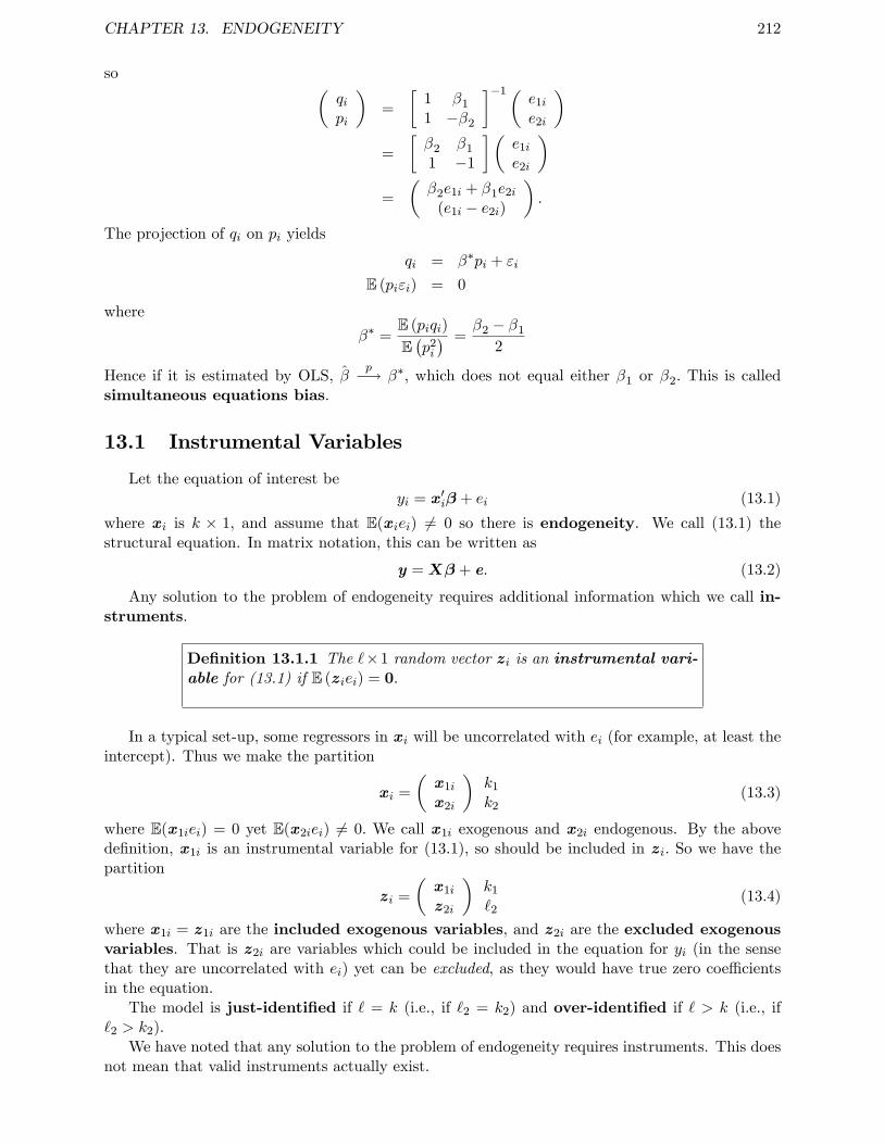
CHAPTER 13. ENDOGENEITY 212
so (qipi
)=
[1 β1
1 −β2
]−1(e1i
e2i
)=
[β2 β1
1 −1
](e1i
e2i
)=
(β2e1i + β1e2i
(e1i − e2i)
).
The projection of qi on pi yields
qi = β∗pi + εi
E (piεi) = 0
where
β∗ =E (piqi)
E(p2i
) =β2 − β1
2
Hence if it is estimated by OLS, βp−→ β∗, which does not equal either β1 or β2. This is called
simultaneous equations bias.
13.1 Instrumental Variables
Let the equation of interest beyi = x′iβ + ei (13.1)
where xi is k × 1, and assume that E(xiei) 6= 0 so there is endogeneity. We call (13.1) thestructural equation. In matrix notation, this can be written as
y = Xβ + e. (13.2)
Any solution to the problem of endogeneity requires additional information which we call in-struments.
Definition 13.1.1 The `×1 random vector zi is an instrumental vari-able for (13.1) if E (ziei) = 0.
In a typical set-up, some regressors in xi will be uncorrelated with ei (for example, at least theintercept). Thus we make the partition
xi =
(x1i
x2i
)k1
k2(13.3)
where E(x1iei) = 0 yet E(x2iei) 6= 0. We call x1i exogenous and x2i endogenous. By the abovedefinition, x1i is an instrumental variable for (13.1), so should be included in zi. So we have thepartition
zi =
(x1i
z2i
)k1
`2(13.4)
where x1i = z1i are the included exogenous variables, and z2i are the excluded exogenousvariables. That is z2i are variables which could be included in the equation for yi (in the sensethat they are uncorrelated with ei) yet can be excluded, as they would have true zero coeffi cientsin the equation.
The model is just-identified if ` = k (i.e., if `2 = k2) and over-identified if ` > k (i.e., if`2 > k2).
We have noted that any solution to the problem of endogeneity requires instruments. This doesnot mean that valid instruments actually exist.
CHAPTER 13. ENDOGENEITY 213
13.2 Reduced Form
The reduced form relationship between the variables or “regressors”xi and the instruments ziis found by linear projection. Let
Γ = E(ziz′i
)−1 E(zix
′i
)be the `× k matrix of coeffi cients from a projection of xi on zi, and define
ui = xi − Γ′zi
as the projection error. Then the reduced form linear relationship between xi and zi is
xi = Γ′zi + ui. (13.5)
In matrix notation, we can write (13.5) as
X = ZΓ +U (13.6)
where U is n× k.By construction,
E(ziu′i) = 0,
so (13.5) is a projection and can be estimated by OLS:
x = zΓ + u
Γ =(z′z)−1 (
z′x).
Substituting (13.6) into (13.2), we find
y = (ZΓ +U)β + e
= Zλ+ v, (13.7)
whereλ = Γβ (13.8)
andv = Uβ + e.
Observe thatE (zivi) = E
(ziu
′i
)β + E (ziei) = 0.
Thus (13.7) is a projection equation and may be estimated by OLS. This is
y = Zλ+ v,
λ =(Z ′Z
)−1 (Z ′y
)The equation (13.7) is the reduced form for y. (13.6) and (13.7) together are the reduced form
equations for the system
y = Zλ+ v
x = ZΓ +U .
As we showed above, OLS yields the reduced-form estimates(λ, Γ
)
CHAPTER 13. ENDOGENEITY 214
13.3 Identification
The structural parameter β relates to (λ,Γ) through (13.8). The parameter β is identified,meaning that it can be recovered from the reduced form, if
rank (Γ) = k. (13.9)
Assume that (13.9) holds. If ` = k, then β = Γ−1λ. If ` > k, then for any W > 0, β =(Γ′WΓ)
−1Γ′Wλ.
If (13.9) is not satisfied, then β cannot be recovered from (λ,Γ) . Note that a necessary (althoughnot suffi cient) condition for (13.9) is ` ≥ k.
Since Z and X have the common variables X1, we can rewrite some of the expressions. Using(13.3) and (13.4) to make the matrix partitions Z = [Z1,Z2] and X = [Z1,X2] , we can partitionΓ as
Γ =
[Γ11 Γ12
Γ21 Γ22
]=
[I Γ12
0 Γ22
](13.6) can be rewritten as
X1 = Z1
X2 = Z1Γ12 +Z2Γ22 +U2. (13.10)
β is identified if rank(Γ) = k, which is true if and only if rank(Γ22) = k2 (by the upper-diagonalstructure of Γ). Thus the key to identification of the model rests on the `2 × k2 matrix Γ22 in(13.10).
13.4 Estimation
The model can be written as
yi = x′iβ + ei
E (ziei) = 0
or
Egi (β) = 0
gi (β) = zi(yi − x′iβ
).
This is a moment condition model. Appropriate estimators include GMM and EL. The estimatorsand distribution theory developed in those Chapter 8 and 9 directly apply. Recall that the GMMestimator, for given weight matrix W n, is
β =(X ′ZW nZ
′X)−1
X ′ZW nZ′y.
13.5 Special Cases: IV and 2SLS
If the model is just-identified, so that k = `, then the formula for GMM simplifies. We find that
β =(X ′ZW nZ
′X)−1
X ′ZW nZ′y
=(Z ′X
)−1W−1
n
(X ′Z
)−1X ′ZW nZ
′y
=(Z ′X
)−1Z ′y
CHAPTER 13. ENDOGENEITY 215
This estimator is often called the instrumental variables estimator (IV) of β, where Z is usedas an instrument forX. Observe that the weight matrixW n has disappeared. In the just-identifiedcase, the weight matrix places no role. This is also the MME estimator of β, and the EL estimator.Another interpretation stems from the fact that since β = Γ−1λ, we can construct the IndirectLeast Squares (ILS) estimator:
β = Γ−1λ
=((Z ′Z
)−1 (Z ′X
))−1 ((Z ′Z
)−1 (Z ′y
))=
(Z ′X
)−1 (Z ′Z
) (Z ′Z
)−1 (Z ′y
)=
(Z ′X
)−1 (Z ′y
).
which again is the IV estimator.
Recall that the optimal weight matrix is an estimate of the inverse of Ω = E(ziz′ie
2i
). In the
special case that E(e2i | zi
)= σ2 (homoskedasticity), then Ω = E (ziz
′i)σ
2 ∝ E (ziz′i) suggesting
the weight matrix W n = (Z ′Z)−1. Using this choice, the GMM estimator equals
β2SLS =(X ′Z
(Z ′Z
)−1Z ′X
)−1X ′Z
(Z ′Z
)−1Z ′y
This is called the two-stage-least squares (2SLS) estimator. It was originally proposed by Theil(1953) and Basmann (1957), and is the classic estimator for linear equations with instruments.Under the homoskedasticity assumption, the 2SLS estimator is effi cient GMM, but otherwise it isineffi cient.
It is useful to observe that writing
P = Z(Z ′Z
)−1Z ′
X = PX = ZΓ
then the 2SLS estimator is
β =(X ′PX
)−1X ′Py
=(X′X)−1
X′y.
The source of the “two-stage”name is since it can be computed as follows
• First regress X on Z, vis., Γ = (Z ′Z)−1
(Z ′X) and X = ZΓ = PX.
• Second, regress y on X, vis., β =(X′X)−1
X′y.
It is useful to scrutinize the projection X. Recall, X = [X1,X2] and Z = [X1,Z2]. Then
X =[X1, X2
]= [PX1,PX2]
= [X1,PX2]
=[X1, X2
],
since X1 lies in the span of X. Thus in the second stage, we regress y on X1 and X2. So only theendogenous variables X2 are replaced by their fitted values:
X2 = Z1Γ12 +Z2Γ22.
CHAPTER 13. ENDOGENEITY 216
13.6 Bekker Asymptotics
Bekker (1994) used an alternative asymptotic framework to analyze the finite-sample bias inthe 2SLS estimator. Here we present a simplified version of one of his results. In our notation, themodel is
y = Xβ + e (13.11)
X = ZΓ +U (13.12)
ξ = (e,U)
E (ξ | Z) = 0
E(ξ′ξ | Z
)= S
As before, Z is n× l so there are l instruments.First, let’s analyze the approximate bias of OLS applied to (13.11). Using (13.12),
E(
1
nX ′e
)= E (xiei) = Γ′E (ziei) + E (uiei) = s21
and
E(
1
nX ′X
)= E
(xix
′i
)= Γ′E
(ziz′i
)Γ + E
(uiz
′i
)Γ + Γ′E
(ziu
′i
)+ E
(uiu
′i
)= Γ′QΓ + S22
where Q = E (ziz′i) . Hence by a first-order approximation
E(βOLS − β
)≈
(E(
1
nX ′X
))−1
E(
1
nX ′e
)=
(Γ′QΓ + S22
)−1s21 (13.13)
which is zero only when s21 = 0 (when X is exogenous).We now derive a similar result for the 2SLS estimator.
β2SLS =(X ′PX
)−1 (X ′Py
).
Let P = Z (Z ′Z)−1Z ′. By the spectral decomposition of an idempotent matrix, P = HΛH ′
where Λ = diag (I l,0) . Let Q = H ′ξS−1/2 which satisfies EQ′Q = In and partition Q = (q′1 Q′2)
where q1 is l × 1. Hence
E(
1
nξ′Pξ | Z
)=
1
nS1/2′E
(Q′ΛQ | Z
)S1/2
=1
nS1/2′E
(1
nq′1q1
)S1/2
=l
nS1/2′S1/2
= αS
where
α =l
n.
Using (13.12) and this result,
1
nE(X ′Pe
)=
1
nE(Γ′Z ′e
)+
1
nE(U ′Pe
)= αs21,
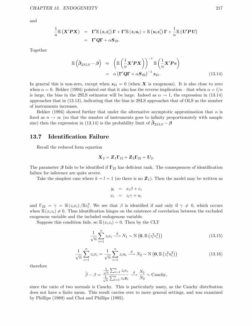
CHAPTER 13. ENDOGENEITY 217
and
1
nE(X ′PX
)= Γ′E
(ziz′i
)Γ + Γ′E (ziui) + E
(uiz
′i
)Γ +
1
nE(U ′PU
)= Γ′QΓ + αS22.
Together
E(β2SLS − β
)≈
(E(
1
nX ′PX
))−1
E(
1
nX ′Pe
)= α
(Γ′QΓ + αS22
)−1s21. (13.14)
In general this is non-zero, except when s21 = 0 (when X is exogenous). It is also close to zerowhen α = 0. Bekker (1994) pointed out that it also has the reverse implication —that when α = l/nis large, the bias in the 2SLS estimator will be large. Indeed as α → 1, the expression in (13.14)approaches that in (13.13), indicating that the bias in 2SLS approaches that of OLS as the numberof instruments increases.
Bekker (1994) showed further that under the alternative asymptotic approximation that α isfixed as n → ∞ (so that the number of instruments goes to infinity proportionately with samplesize) then the expression in (13.14) is the probability limit of β2SLS − β
13.7 Identification Failure
Recall the reduced form equation
X2 = Z1Γ12 +Z2Γ22 +U2.
The parameter β fails to be identified if Γ22 has deficient rank. The consequences of identificationfailure for inference are quite severe.
Take the simplest case where k = l = 1 (so there is no Z1). Then the model may be written as
yi = xiβ + ei
xi = ziγ + ui
and Γ22 = γ = E (zixi) /Ez2i . We see that β is identified if and only if γ 6= 0, which occurs
when E (xizi) 6= 0. Thus identification hinges on the existence of correlation between the excludedexogenous variable and the included endogenous variable.
Suppose this condition fails, so E (xizi) = 0. Then by the CLT
1√n
n∑i=1
zieid−→ N1 ∼ N
(0,E
(z2i e
2i
))(13.15)
1√n
n∑i=1
zixi =1√n
n∑i=1
ziuid−→ N2 ∼ N
(0,E
(z2i u
2i
))(13.16)
therefore
β − β =
1√n
∑ni=1 ziei
1√n
∑ni=1 zixi
d−→ N1
N2∼ Cauchy,
since the ratio of two normals is Cauchy. This is particularly nasty, as the Cauchy distributiondoes not have a finite mean. This result carries over to more general settings, and was examinedby Phillips (1989) and Choi and Phillips (1992).
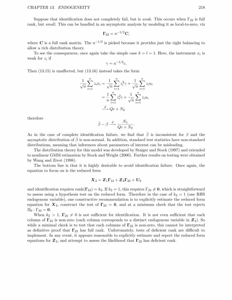
CHAPTER 13. ENDOGENEITY 218
Suppose that identification does not completely fail, but is weak. This occurs when Γ22 is fullrank, but small. This can be handled in an asymptotic analysis by modeling it as local-to-zero, viz
Γ22 = n−1/2C,
where C is a full rank matrix. The n−1/2 is picked because it provides just the right balancing toallow a rich distribution theory.
To see the consequences, once again take the simple case k = l = 1. Here, the instrument xi isweak for zi if
γ = n−1/2c.
Then (13.15) is unaffected, but (13.16) instead takes the form
1√n
n∑i=1
zixi =1√n
n∑i=1
z2i γ +
1√n
n∑i=1
ziui
=1
n
n∑i=1
z2i c+
1√n
n∑i=1
ziui
d−→ Qc+N2
therefore
β − β d−→ N1
Qc+N2.
As in the case of complete identification failure, we find that β is inconsistent for β and theasymptotic distribution of β is non-normal. In addition, standard test statistics have non-standarddistributions, meaning that inferences about parameters of interest can be misleading.
The distribution theory for this model was developed by Staiger and Stock (1997) and extendedto nonlinear GMM estimation by Stock and Wright (2000). Further results on testing were obtainedby Wang and Zivot (1998).
The bottom line is that it is highly desirable to avoid identification failure. Once again, theequation to focus on is the reduced form
X2 = Z1Γ12 +Z2Γ22 +U2
and identification requires rank(Γ22) = k2. If k2 = 1, this requires Γ22 6= 0, which is straightforwardto assess using a hypothesis test on the reduced form. Therefore in the case of k2 = 1 (one RHSendogenous variable), one constructive recommendation is to explicitly estimate the reduced formequation for X2, construct the test of Γ22 = 0, and at a minimum check that the test rejectsH0 : Γ22 = 0.
When k2 > 1, Γ22 6= 0 is not suffi cient for identification. It is not even suffi cient that eachcolumn of Γ22 is non-zero (each column corresponds to a distinct endogenous variable in Z2). Sowhile a minimal check is to test that each columns of Γ22 is non-zero, this cannot be interpretedas definitive proof that Γ22 has full rank. Unfortunately, tests of deficient rank are diffi cult toimplement. In any event, it appears reasonable to explicitly estimate and report the reduced formequations for Z2, and attempt to assess the likelihood that Γ22 has deficient rank.
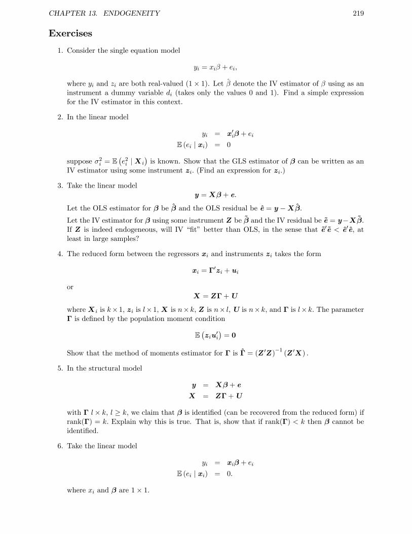
CHAPTER 13. ENDOGENEITY 219
Exercises
1. Consider the single equation model
yi = xiβ + ei,
where yi and zi are both real-valued (1× 1). Let β denote the IV estimator of β using as aninstrument a dummy variable di (takes only the values 0 and 1). Find a simple expressionfor the IV estimator in this context.
2. In the linear model
yi = x′iβ + ei
E (ei | xi) = 0
suppose σ2i = E
(e2i |Xi
)is known. Show that the GLS estimator of β can be written as an
IV estimator using some instrument zi. (Find an expression for zi.)
3. Take the linear modely = Xβ + e.
Let the OLS estimator for β be β and the OLS residual be e = y −Xβ.Let the IV estimator for β using some instrument Z be β and the IV residual be e = y−Xβ.If Z is indeed endogeneous, will IV “fit” better than OLS, in the sense that e′e < e′e, atleast in large samples?
4. The reduced form between the regressors xi and instruments zi takes the form
xi = Γ′zi + ui
orX = ZΓ +U
where Xi is k×1, zi is l×1, X is n×k, Z is n× l, U is n×k, and Γ is l×k. The parameterΓ is defined by the population moment condition
E(ziu
′i
)= 0
Show that the method of moments estimator for Γ is Γ = (Z ′Z)−1
(Z ′X) .
5. In the structural model
y = Xβ + e
X = ZΓ +U
with Γ l× k, l ≥ k, we claim that β is identified (can be recovered from the reduced form) ifrank(Γ) = k. Explain why this is true. That is, show that if rank(Γ) < k then β cannot beidentified.
6. Take the linear model
yi = xiβ + ei
E (ei | xi) = 0.
where xi and β are 1× 1.
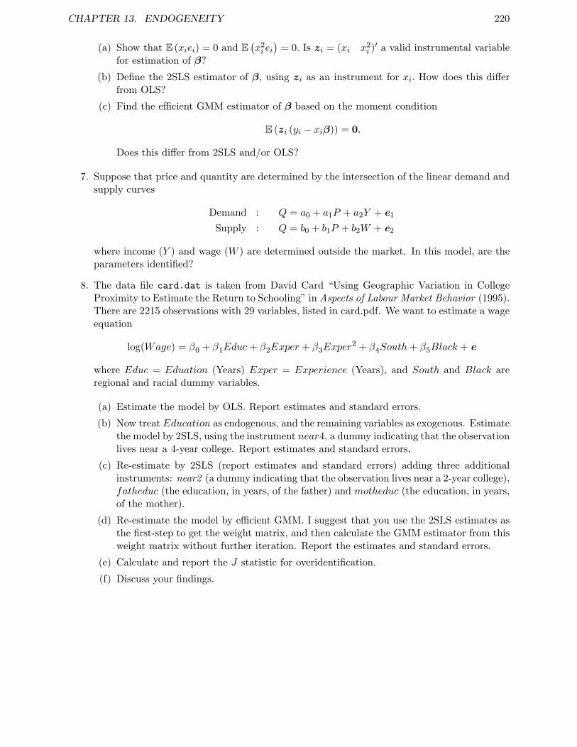
CHAPTER 13. ENDOGENEITY 220
(a) Show that E (xiei) = 0 and E(x2i ei)
= 0. Is zi = (xi x2i )′ a valid instrumental variable
for estimation of β?
(b) Define the 2SLS estimator of β, using zi as an instrument for xi. How does this differfrom OLS?
(c) Find the effi cient GMM estimator of β based on the moment condition
E (zi (yi − xiβ)) = 0.
Does this differ from 2SLS and/or OLS?
7. Suppose that price and quantity are determined by the intersection of the linear demand andsupply curves
Demand : Q = a0 + a1P + a2Y + e1
Supply : Q = b0 + b1P + b2W + e2
where income (Y ) and wage (W ) are determined outside the market. In this model, are theparameters identified?
8. The data file card.dat is taken from David Card “Using Geographic Variation in CollegeProximity to Estimate the Return to Schooling”in Aspects of Labour Market Behavior (1995).There are 2215 observations with 29 variables, listed in card.pdf. We want to estimate a wageequation
log(Wage) = β0 + β1Educ+ β2Exper + β3Exper2 + β4South+ β5Black + e
where Educ = Eduation (Years) Exper = Experience (Years), and South and Black areregional and racial dummy variables.
(a) Estimate the model by OLS. Report estimates and standard errors.
(b) Now treat Education as endogenous, and the remaining variables as exogenous. Estimatethe model by 2SLS, using the instrument near4, a dummy indicating that the observationlives near a 4-year college. Report estimates and standard errors.
(c) Re-estimate by 2SLS (report estimates and standard errors) adding three additionalinstruments: near2 (a dummy indicating that the observation lives near a 2-year college),fatheduc (the education, in years, of the father) and motheduc (the education, in years,of the mother).
(d) Re-estimate the model by effi cient GMM. I suggest that you use the 2SLS estimates asthe first-step to get the weight matrix, and then calculate the GMM estimator from thisweight matrix without further iteration. Report the estimates and standard errors.
(e) Calculate and report the J statistic for overidentification.
(f) Discuss your findings.
Chapter 14
Univariate Time Series
A time series yt is a process observed in sequence over time, t = 1, ..., T . To indicate thedependence on time, we adopt new notation, and use the subscript t to denote the individualobservation, and T to denote the number of observations.
Because of the sequential nature of time series, we expect that yt and yt−1 are not independent,so classical assumptions are not valid.
We can separate time series into two categories: univariate (yt ∈ R is scalar); and multivariate(yt ∈ Rm is vector-valued). The primary model for univariate time series is autoregressions (ARs).The primary model for multivariate time series is vector autoregressions (VARs).
14.1 Stationarity and Ergodicity
Definition 14.1.1 yt is covariance (weakly) stationary if
E(yt) = µ
is independent of t, and
cov (yt, yt−k) = γ(k)
is independent of t for all k.γ(k) is called the autocovariance function.
ρ(k) = γ(k)/γ(0) = corr(yt, yt−k)
is the autocorrelation function.
Definition 14.1.2 yt is strictly stationary if the joint distribution of(yt, ..., yt−k) is independent of t for all k.
Definition 14.1.3 A stationary time series is ergodic if γ(k) → 0 ask →∞.
221
CHAPTER 14. UNIVARIATE TIME SERIES 222
The following two theorems are essential to the analysis of stationary time series. There proofsare rather diffi cult, however.
Theorem 14.1.1 If yt is strictly stationary and ergodic and xt =f(yt, yt−1, ...) is a random variable, then xt is strictly stationary and er-godic.
Theorem 14.1.2 (Ergodic Theorem). If yt is strictly stationary and er-godic and E |yt| <∞, then as T →∞,
1
T
T∑t=1
ytp−→ E(yt).
This allows us to consistently estimate parameters using time-series moments:The sample mean:
µ =1
T
T∑t=1
yt
The sample autocovariance
γ(k) =1
T
T∑t=1
(yt − µ) (yt−k − µ) .
The sample autocorrelation
ρ(k) =γ(k)
γ(0).
Theorem 14.1.3 If yt is strictly stationary and ergodic and Ey2t < ∞,
then as T →∞,
1. µp−→ E(yt);
2. γ(k)p−→ γ(k);
3. ρ(k)p−→ ρ(k).
Proof of Theorem 14.1.3. Part (1) is a direct consequence of the Ergodic theorem. For Part(2), note that
γ(k) =1
T
T∑t=1
(yt − µ) (yt−k − µ)
=1
T
T∑t=1
ytyt−k −1
T
T∑t=1
ytµ−1
T
T∑t=1
yt−kµ+ µ2.
CHAPTER 14. UNIVARIATE TIME SERIES 223
By Theorem 14.1.1 above, the sequence ytyt−k is strictly stationary and ergodic, and it has a finitemean by the assumption that Ey2
t <∞. Thus an application of the Ergodic Theorem yields
1
T
T∑t=1
ytyt−kp−→ E(ytyt−k).
Thusγ(k)
p−→ E(ytyt−k)− µ2 − µ2 + µ2 = E(ytyt−k)− µ2 = γ(k).
Part (3) follows by the continuous mapping theorem: ρ(k) = γ(k)/γ(0)p−→ γ(k)/γ(0) = ρ(k).
14.2 Autoregressions
In time-series, the series ..., y1, y2, ..., yT , ... are jointly random. We consider the conditionalexpectation
E (yt | Ft−1)
where Ft−1 = yt−1, yt−2, ... is the past history of the series.An autoregressive (AR) model specifies that only a finite number of past lags matter:
E (yt | Ft−1) = E (yt | yt−1, ..., yt−k) .
A linear AR model (the most common type used in practice) specifies linearity:
E (yt | Ft−1) = α+ ρ1yt−1 + ρ2yt−1 + · · ·+ ρkyt−k.
Lettinget = yt − E (yt | Ft−1) ,
then we have the autoregressive model
yt = α+ ρ1yt−1 + ρ2yt−1 + · · ·+ ρkyt−k + et
E (et | Ft−1) = 0.
The last property defines a special time-series process.
Definition 14.2.1 et is a martingale diff erence sequence (MDS) ifE (et | Ft−1) = 0.
Regression errors are naturally a MDS. Some time-series processes may be a MDS as a conse-quence of optimizing behavior. For example, some versions of the life-cycle hypothesis imply thateither changes in consumption, or consumption growth rates, should be a MDS. Most asset pricingmodels imply that asset returns should be the sum of a constant plus a MDS.
The MDS property for the regression error plays the same role in a time-series regression asdoes the conditional mean-zero property for the regression error in a cross-section regression. Infact, it is even more important in the time-series context, as it is diffi cult to derive distributiontheories without this property.
A useful property of a MDS is that et is uncorrelated with any function of the lagged informationFt−1. Thus for k > 0, E (yt−ket) = 0.
CHAPTER 14. UNIVARIATE TIME SERIES 224
14.3 Stationarity of AR(1) Process
A mean-zero AR(1) isyt = ρyt−1 + et.
Assume that et is iid, E(et) = 0 and Ee2t = σ2 <∞.
By back-substitution, we find
yt = et + ρet−1 + ρ2et−2 + ...
=
∞∑k=0
ρket−k.
Loosely speaking, this series converges if the sequence ρket−k gets small as k → ∞. This occurswhen |ρ| < 1.
Theorem 14.3.1 If and only if |ρ| < 1 then yt is strictly stationary andergodic.
We can compute the moments of yt using the infinite sum:
Eyt =∞∑k=0
ρkE (et−k) = 0
var(yt) =∞∑k=0
ρ2k var (et−k) =σ2
1− ρ2.
If the equation for yt has an intercept, the above results are unchanged, except that the meanof yt can be computed from the relationship
Eyt = α+ ρEyt−1,
and solving for Eyt = Eyt−1 we find Eyt = α/(1− ρ).
14.4 Lag Operator
An algebraic construct which is useful for the analysis of autoregressive models is the lag oper-ator.
Definition 14.4.1 The lag operator L satisfies Lyt = yt−1.
Defining L2 = LL, we see that L2yt = Lyt−1 = yt−2. In general, Lkyt = yt−k.The AR(1) model can be written in the format
yt − ρyt−1 = et
or(1− ρL) yt = et.
The operator ρ(L) = (1 − ρL) is a polynomial in the operator L. We say that the root of thepolynomial is 1/ρ, since ρ(z) = 0 when z = 1/ρ. We call ρ(L) the autoregressive polynomial of yt.
From Theorem 14.3.1, an AR(1) is stationary iff |ρ| < 1. Note that an equivalent way to saythis is that an AR(1) is stationary iff the root of the autoregressive polynomial is larger than one(in absolute value).
CHAPTER 14. UNIVARIATE TIME SERIES 225
14.5 Stationarity of AR(k)
The AR(k) model isyt = ρ1yt−1 + ρ2yt−2 + · · ·+ ρkyt−k + et.
Using the lag operator,yt − ρ1Lyt − ρ2L2yt − · · · − ρkLkyt = et,
orρ(L)yt = et
whereρ(L) = 1− ρ1L− ρ2L2 − · · · − ρkLk.
We call ρ(L) the autoregressive polynomial of yt.The Fundamental Theorem of Algebra says that any polynomial can be factored as
ρ(z) =(1− λ−1
1 z) (
1− λ−12 z)· · ·(1− λ−1
k z)
where the λ1, ..., λk are the complex roots of ρ(z), which satisfy ρ(λj) = 0.We know that an AR(1) is stationary iff the absolute value of the root of its autoregressive
polynomial is larger than one. For an AR(k), the requirement is that all roots are larger than one.Let |λ| denote the modulus of a complex number λ.
Theorem 14.5.1 The AR(k) is strictly stationary and ergodic if and onlyif |λj | > 1 for all j.
One way of stating this is that “All roots lie outside the unit circle.”If one of the roots equals 1, we say that ρ(L), and hence yt, “has a unit root”. This is a special
case of non-stationarity, and is of great interest in applied time series.
14.6 Estimation
Let
xt =(
1 yt−1 yt−2 · · · yt−k)′
β =(α ρ1 ρ2 · · · ρk
)′.
Then the model can be written asyt = x′tβ + et.
The OLS estimator isβ =
(X ′X
)−1X ′y.
To study β, it is helpful to define the process ut = xtet. Note that ut is a MDS, since
E (ut | Ft−1) = E (xtet | Ft−1) = xtE (et | Ft−1) = 0.
By Theorem 14.1.1, it is also strictly stationary and ergodic. Thus
1
T
T∑t=1
xtet =1
T
T∑t=1
utp−→ E (ut) = 0. (14.1)
CHAPTER 14. UNIVARIATE TIME SERIES 226
The vector xt is strictly stationary and ergodic, and by Theorem 14.1.1, so is xtx′t. Thus by theErgodic Theorem,
1
T
T∑t=1
xtx′t
p−→ E(xtx
′t
)= Q.
Combined with (14.1) and the continuous mapping theorem, we see that
β = β +
(1
T
T∑t=1
xtx′t
)−1(1
T
T∑t=1
xtet
)p−→ Q−10 = 0.
We have shown the following:
Theorem 14.6.1 If the AR(k) process yt is strictly stationary and ergodicand Ey2
t <∞, then βp−→ β as T →∞.
14.7 Asymptotic Distribution
Theorem 14.7.1 MDS CLT. If ut is a strictly stationary and ergodicMDS and E (utu
′t) = Ω <∞, then as T →∞,
1√T
T∑t=1
utd−→ N (0,Ω) .
Since xtet is a MDS, we can apply Theorem 14.7.1 to see that
1√T
T∑t=1
xtetd−→ N (0,Ω) ,
whereΩ = E(xtx
′te
2t ).
Theorem 14.7.2 If the AR(k) process yt is strictly stationary and ergodicand Ey4
t <∞, then as T →∞,√T(β − β
)d−→ N
(0,Q−1ΩQ−1
).
This is identical in form to the asymptotic distribution of OLS in cross-section regression. Theimplication is that asymptotic inference is the same. In particular, the asymptotic covariancematrix is estimated just as in the cross-section case.
CHAPTER 14. UNIVARIATE TIME SERIES 227
14.8 Bootstrap for Autoregressions
In the non-parametric bootstrap, we constructed the bootstrap sample by randomly resamplingfrom the data values yt,xt. This creates an iid bootstrap sample. Clearly, this cannot work in atime-series application, as this imposes inappropriate independence.
Briefly, there are two popular methods to implement bootstrap resampling for time-series data.
Method 1: Model-Based (Parametric) Bootstrap.
1. Estimate β and residuals et.
2. Fix an initial condition (y−k+1, y−k+2, ..., y0).
3. Simulate iid draws e∗i from the empirical distribution of the residuals e1, ..., eT .
4. Create the bootstrap series y∗t by the recursive formula
y∗t = α+ ρ1y∗t−1 + ρ2y
∗t−2 + · · ·+ ρky
∗t−k + e∗t .
This construction imposes homoskedasticity on the errors e∗i , which may be different than theproperties of the actual ei. It also presumes that the AR(k) structure is the truth.
Method 2: Block Resampling
1. Divide the sample into T/m blocks of length m.
2. Resample complete blocks. For each simulated sample, draw T/m blocks.
3. Paste the blocks together to create the bootstrap time-series y∗t .
4. This allows for arbitrary stationary serial correlation, heteroskedasticity, and for model-misspecification.
5. The results may be sensitive to the block length, and the way that the data are partitionedinto blocks.
6. May not work well in small samples.
14.9 Trend Stationarity
yt = µ0 + µ1t+ St (14.2)
St = ρ1St−1 + ρ2St−2 + · · ·+ ρkSt−l + et, (14.3)
oryt = α0 + α1t+ ρ1yt−1 + ρ2yt−1 + · · ·+ ρkyt−k + et. (14.4)
There are two essentially equivalent ways to estimate the autoregressive parameters (ρ1, ..., ρk).
• You can estimate (14.4) by OLS.
• You can estimate (14.2)-(14.3) sequentially by OLS. That is, first estimate (14.2), get theresidual St, and then perform regression (14.3) replacing St with St. This procedure is some-times called Detrending.
CHAPTER 14. UNIVARIATE TIME SERIES 228
The reason why these two procedures are (essentially) the same is the Frisch-Waugh-Lovelltheorem.
Seasonal Effects
There are three popular methods to deal with seasonal data.
• Include dummy variables for each season. This presumes that “seasonality”does not changeover the sample.
• Use “seasonally adjusted” data. The seasonal factor is typically estimated by a two-sidedweighted average of the data for that season in neighboring years. Thus the seasonallyadjusted data is a “filtered”series. This is a flexible approach which can extract a wide rangeof seasonal factors. The seasonal adjustment, however, also alters the time-series correlationsof the data.
• First apply a seasonal differencing operator. If s is the number of seasons (typically s = 4 ors = 12),
∆syt = yt − yt−s,or the season-to-season change. The series ∆syt is clearly free of seasonality. But the long-runtrend is also eliminated, and perhaps this was of relevance.
14.10 Testing for Omitted Serial Correlation
For simplicity, let the null hypothesis be an AR(1):
yt = α+ ρyt−1 + ut. (14.5)
We are interested in the question if the error ut is serially correlated. We model this as an AR(1):
ut = θut−1 + et (14.6)
with et a MDS. The hypothesis of no omitted serial correlation is
H0 : θ = 0
H1 : θ 6= 0.
We want to test H0 against H1.To combine (14.5) and (14.6), we take (14.5) and lag the equation once:
yt−1 = α+ ρyt−2 + ut−1.
We then multiply this by θ and subtract from (14.5), to find
yt − θyt−1 = α− θα+ ρyt−1 − θρyt−1 + ut − θut−1,
oryt = α(1− θ) + (ρ+ θ) yt−1 − θρyt−2 + et = AR(2).
Thus under H0, yt is an AR(1), and under H1 it is an AR(2). H0 may be expressed as the restrictionthat the coeffi cient on yt−2 is zero.
An appropriate test of H0 against H1 is therefore a Wald test that the coeffi cient on yt−2 iszero. (A simple exclusion test).
In general, if the null hypothesis is that yt is an AR(k), and the alternative is that the error is anAR(m), this is the same as saying that under the alternative yt is an AR(k+m), and this is equivalentto the restriction that the coeffi cients on yt−k−1, ..., yt−k−m are jointly zero. An appropriate test isthe Wald test of this restriction.
CHAPTER 14. UNIVARIATE TIME SERIES 229
14.11 Model Selection
What is the appropriate choice of k in practice? This is a problem of model selection.One approach to model selection is to choose k based on a Wald tests.Another is to minimize the AIC or BIC information criterion, e.g.
AIC(k) = log σ2(k) +2k
T,
where σ2(k) is the estimated residual variance from an AR(k)One ambiguity in defining the AIC criterion is that the sample available for estimation changes
as k changes. (If you increase k, you need more initial conditions.) This can induce strangebehavior in the AIC. The best remedy is to fix a upper value k, and then reserve the first k asinitial conditions, and then estimate the models AR(1), AR(2), ..., AR(k) on this (unified) sample.
14.12 Autoregressive Unit Roots
The AR(k) model is
ρ(L)yt = µ+ et
ρ(L) = 1− ρ1L− · · · − ρkLk.
As we discussed before, yt has a unit root when ρ(1) = 0, or
ρ1 + ρ2 + · · ·+ ρk = 1.
In this case, yt is non-stationary. The ergodic theorem and MDS CLT do not apply, and teststatistics are asymptotically non-normal.
A helpful way to write the equation is the so-called Dickey-Fuller reparameterization:
∆yt = µ+ α0yt−1 + α1∆yt−1 + · · ·+ αk−1∆yt−(k−1) + et. (14.7)
These models are equivalent linear transformations of one another. The DF parameterizationis convenient because the parameter α0 summarizes the information about the unit root, sinceρ(1) = −α0. To see this, observe that the lag polynomial for the yt computed from (14.7) is
(1− L)− α0L− α1(L− L2)− · · · − αk−1(Lk−1 − Lk)
But this must equal ρ(L), as the models are equivalent. Thus
ρ(1) = (1− 1)− α0 − (1− 1)− · · · − (1− 1) = −α0.
Hence, the hypothesis of a unit root in yt can be stated as
H0 : α0 = 0.
Note that the model is stationary if α0 < 0. So the natural alternative is
H1 : α0 < 0.
Under H0, the model for yt is
∆yt = µ+ α1∆yt−1 + · · ·+ αk−1∆yt−(k−1) + et,
which is an AR(k-1) in the first-difference ∆yt. Thus if yt has a (single) unit root, then ∆yt is astationary AR process. Because of this property, we say that if yt is non-stationary but ∆dyt isstationary, then yt is “integrated of order d”, or I(d). Thus a time series with unit root is I(1).
CHAPTER 14. UNIVARIATE TIME SERIES 230
Since α0 is the parameter of a linear regression, the natural test statistic is the t-statistic forH0 from OLS estimation of (14.7). Indeed, this is the most popular unit root test, and is called theAugmented Dickey-Fuller (ADF) test for a unit root.
It would seem natural to assess the significance of the ADF statistic using the normal table.However, under H0, yt is non-stationary, so conventional normal asymptotics are invalid. Analternative asymptotic framework has been developed to deal with non-stationary data. We do nothave the time to develop this theory in detail, but simply assert the main results.
Theorem 14.12.1 Dickey-Fuller Theorem.Assume α0 = 0. As T →∞,
T α0d−→ (1− α1 − α2 − · · · − αk−1)DFα
ADF =α0
s(α0)→ DFt.
The limit distributions DFα and DFt are non-normal. They are skewed to the left, and havenegative means.
The first result states that α0 converges to its true value (of zero) at rate T, rather than theconventional rate of T 1/2. This is called a “super-consistent”rate of convergence.
The second result states that the t-statistic for α0 converges to a limit distribution which isnon-normal, but does not depend on the parameters α. This distribution has been extensivelytabulated, and may be used for testing the hypothesis H0. Note: The standard error s(α0) is theconventional (“homoskedastic”) standard error. But the theorem does not require an assumptionof homoskedasticity. Thus the Dickey-Fuller test is robust to heteroskedasticity.
Since the alternative hypothesis is one-sided, the ADF test rejects H0 in favor of H1 whenADF < c, where c is the critical value from the ADF table. If the test rejects H0, this means thatthe evidence points to yt being stationary. If the test does not reject H0, a common conclusion isthat the data suggests that yt is non-stationary. This is not really a correct conclusion, however.All we can say is that there is insuffi cient evidence to conclude whether the data are stationary ornot.
We have described the test for the setting of with an intercept. Another popular setting includesas well a linear time trend. This model is
∆yt = µ1 + µ2t+ α0yt−1 + α1∆yt−1 + · · ·+ αk−1∆yt−(k−1) + et. (14.8)
This is natural when the alternative hypothesis is that the series is stationary about a linear timetrend. If the series has a linear trend (e.g. GDP, Stock Prices), then the series itself is non-stationary, but it may be stationary around the linear time trend. In this context, it is a silly wasteof time to fit an AR model to the level of the series without a time trend, as the AR model cannotconceivably describe this data. The natural solution is to include a time trend in the fitted OLSequation. When conducting the ADF test, this means that it is computed as the t-ratio for α0 fromOLS estimation of (14.8).
If a time trend is included, the test procedure is the same, but different critical values arerequired. The ADF test has a different distribution when the time trend has been included, and adifferent table should be consulted.
Most texts include as well the critical values for the extreme polar case where the intercept hasbeen omitted from the model. These are included for completeness (from a pedagogical perspective)but have no relevance for empirical practice where intercepts are always included.
Chapter 15
Multivariate Time Series
A multivariate time series yt is a vector process m×1. Let Ft−1 = (yt−1,yt−2, ...) be all laggedinformation at time t. The typical goal is to find the conditional expectation E (yt | Ft−1) . Notethat since yt is a vector, this conditional expectation is also a vector.
15.1 Vector Autoregressions (VARs)
A VAR model specifies that the conditional mean is a function of only a finite number of lags:
E (yt | Ft−1) = E(yt | yt−1, ...,yt−k
).
A linear VAR specifies that this conditional mean is linear in the arguments:
E(yt | yt−1, ...,yt−k
)= a0 +A1yt−1 +A2yt−2 + · · ·Akyt−k.
Observe that a0 is m× 1,and each of A1 through Ak are m×m matrices.Defining the m× 1 regression error
et = yt − E (yt | Ft−1) ,
we have the VAR model
yt = a0 +A1yt−1 +A2yt−2 + · · ·Akyt−k + et
E (et | Ft−1) = 0.
Alternatively, defining the mk + 1 vector
xt =
1yt−1
yt−2...
yt−k
and the m× (mk + 1) matrix
A =(a0 A1 A2 · · · Ak
),
thenyt = Axt + et.
The VAR model is a system of m equations. One way to write this is to let a′j be the jth rowof A. Then the VAR system can be written as the equations
Yjt = a′jxt + ejt.
Unrestricted VARs were introduced to econometrics by Sims (1980).
231
CHAPTER 15. MULTIVARIATE TIME SERIES 232
15.2 Estimation
Consider the moment conditionsE (xtejt) = 0,
j = 1, ...,m. These are implied by the VAR model, either as a regression, or as a linear projection.The GMM estimator corresponding to these moment conditions is equation-by-equation OLS
aj = (X ′X)−1X ′yj .
An alternative way to compute this is as follows. Note that
a′j = y′jX(X ′X)−1.
And if we stack these to create the estimate A, we find
A =
y′1y′2...
y′m+1
X(X ′X)−1
= Y ′X(X ′X)−1,
whereY =
(y1 y2 · · · ym
)the T ×m matrix of the stacked y′t.
This (system) estimator is known as the SUR (Seemingly Unrelated Regressions) estimator,and was originally derived by Zellner (1962)
15.3 Restricted VARs
The unrestricted VAR is a system of m equations, each with the same set of regressors. Arestricted VAR imposes restrictions on the system. For example, some regressors may be excludedfrom some of the equations. Restrictions may be imposed on individual equations, or across equa-tions. The GMM framework gives a convenient method to impose such restrictions on estimation.
15.4 Single Equation from a VAR
Often, we are only interested in a single equation out of a VAR system. This takes the form
yjt = a′jxt + et,
and xt consists of lagged values of yjt and the other y′lts. In this case, it is convenient to re-definethe variables. Let yt = yjt, and zt be the other variables. Let et = ejt and β = aj . Then the singleequation takes the form
yt = x′tβ + et, (15.1)
andxt =
[(1 yt−1 · · · yt−k z′t−1 · · · z′t−k
)′].
This is just a conventional regression with time series data.
CHAPTER 15. MULTIVARIATE TIME SERIES 233
15.5 Testing for Omitted Serial Correlation
Consider the problem of testing for omitted serial correlation in equation (15.1). Suppose thatet is an AR(1). Then
yt = x′tβ + et
et = θet−1 + ut (15.2)
E (ut | Ft−1) = 0.
Then the null and alternative are
H0 : θ = 0 H1 : θ 6= 0.
Take the equation yt = x′tβ + et, and subtract off the equation once lagged multiplied by θ, to get
yt − θyt−1 =(x′tβ + et
)− θ
(x′t−1β + et−1
)= x′tβ − θxt−1β + et − θet−1,
oryt = θyt−1 + x′tβ + x′t−1γ + ut, (15.3)
which is a valid regression model.So testing H0 versus H1 is equivalent to testing for the significance of adding (yt−1,xt−1) to
the regression. This can be done by a Wald test. We see that an appropriate, general, and simpleway to test for omitted serial correlation is to test the significance of extra lagged values of thedependent variable and regressors.
You may have heard of the Durbin-Watson test for omitted serial correlation, which once wasvery popular, and is still routinely reported by conventional regression packages. The DW test isappropriate only when regression yt = x′tβ+ et is not dynamic (has no lagged values on the RHS),and et is iid N(0, σ2). Otherwise it is invalid.
Another interesting fact is that (15.2) is a special case of (15.3), under the restriction γ = −βθ.This restriction, which is called a common factor restriction, may be tested if desired. If valid,the model (15.2) may be estimated by iterated GLS. (A simple version of this estimator is calledCochrane-Orcutt.) Since the common factor restriction appears arbitrary, and is typically rejectedempirically, direct estimation of (15.2) is uncommon in recent applications.
15.6 Selection of Lag Length in an VAR
If you want a data-dependent rule to pick the lag length k in a VAR, you may either use a testing-based approach (using, for example, the Wald statistic), or an information criterion approach. Theformula for the AIC and BIC are
AIC(k) = log det(Ω(k)
)+ 2
p
T
BIC(k) = log det(Ω(k)
)+p log(T )
T
Ω(k) =1
T
T∑t=1
et(k)et(k)′
p = m(km+ 1)
where p is the number of parameters in the model, and et(k) is the OLS residual vector from themodel with k lags. The log determinant is the criterion from the multivariate normal likelihood.
CHAPTER 15. MULTIVARIATE TIME SERIES 234
15.7 Granger Causality
Partition the data vector into (yt, zt). Define the two information sets
F1t =(yt,yt−1,yt−2, ...
)F2t =
(yt, zt,yt−1, zt−1,yt−2, zt−2, , ...
)The information set F1t is generated only by the history of yt, and the information set F2t isgenerated by both yt and zt. The latter has more information.
We say that zt does not Granger-cause yt if
E (yt | F1,t−1) = E (yt | F2,t−1) .
That is, conditional on information in lagged yt, lagged zt does not help to forecast yt. If thiscondition does not hold, then we say that zt Granger-causes yt.
The reason why we call this “Granger Causality”rather than “causality”is because this is nota physical or structure definition of causality. If zt is some sort of forecast of the future, such as afutures price, then zt may help to forecast yt even though it does not “cause”yt. This definitionof causality was developed by Granger (1969) and Sims (1972).
In a linear VAR, the equation for yt is
yt = α+ ρ1yt−1 + · · ·+ ρkyt−k + z′t−1γ1 + · · ·+ z′t−kγk + et.
In this equation, zt does not Granger-cause yt if and only if
H0 : γ1 = γ2 = · · · = γk = 0.
This may be tested using an exclusion (Wald) test.This idea can be applied to blocks of variables. That is, yt and/or zt can be vectors. The
hypothesis can be tested by using the appropriate multivariate Wald test.If it is found that zt does not Granger-cause yt, then we deduce that our time-series model of
E (yt | Ft−1) does not require the use of zt. Note, however, that zt may still be useful to explainother features of yt, such as the conditional variance.
Clive W. J. Granger
Clive Granger (1934-2009) of England was one of the leading figures in time-series econo-metrics, and co-winner in 2003 of the Nobel Memorial Prize in Economic Sciences (alongwith Robert Engle). In addition to formalizing the definition of causality known as Grangercausality, he invented the concept of cointegration, introduced spectral methods into econo-metrics, and formalized methods for the combination of forecasts.
15.8 Cointegration
The idea of cointegration is due to Granger (1981), and was articulated in detail by Engle andGranger (1987).
Definition 15.8.1 The m × 1 series yt is cointegrated if yt is I(1) yetthere exists β, m× r, of rank r, such that zt = β′yt is I(0). The r vectorsin β are called the cointegrating vectors.
CHAPTER 15. MULTIVARIATE TIME SERIES 235
If the series yt is not cointegrated, then r = 0. If r = m, then yt is I(0). For 0 < r < m, yt isI(1) and cointegrated.
In some cases, it may be believed that β is known a priori. Often, β = (1 − 1)′. For example,if yt is a pair of interest rates, then β = (1 − 1)′ specifies that the spread (the difference inreturns) is stationary. If y = (log(Consumption) log(Income))′, then β = (1 − 1)′ specifiesthat log(Consumption/Income) is stationary.
In other cases, β may not be known.If yt is cointegrated with a single cointegrating vector (r = 1), then it turns out that β can
be consistently estimated by an OLS regression of one component of yt on the others. Thus yt =
(Y1t, Y2t) and β = (β1 β2) and normalize β1 = 1. Then β2 = (y′2y2)−1y′2y1p−→ β2. Furthermore
this estimation is super-consistent: T (β2 − β2)d−→ Limit, as first shown by Stock (1987). This
is not, in general, a good method to estimate β, but it is useful in the construction of alternativeestimators and tests.
We are often interested in testing the hypothesis of no cointegration:
H0 : r = 0
H1 : r > 0.
Suppose that β is known, so zt = β′yt is known. Then under H0 zt is I(1), yet under H1 zt isI(0). Thus H0 can be tested using a univariate ADF test on zt.
When β is unknown, Engle and Granger (1987) suggested using an ADF test on the estimatedresidual zt = β
′yt, from OLS of y1t on y2t. Their justification was Stock’s result that β is super-
consistent under H1. Under H0, however, β is not consistent, so the ADF critical values are notappropriate. The asymptotic distribution was worked out by Phillips and Ouliaris (1990).
When the data have time trends, it may be necessary to include a time trend in the estimatedcointegrating regression. Whether or not the time trend is included, the asymptotic distribution ofthe test is affected by the presence of the time trend. The asymptotic distribution was worked outin B. Hansen (1992).
15.9 Cointegrated VARs
We can write a VAR as
A(L)yt = et
A(L) = I −A1L−A2L2 − · · · −AkLk
or alternatively as∆yt = Πyt−1 +D(L)∆yt−1 + et
where
Π = −A(1)
= −I +A1 +A2 + · · ·+Ak.
Theorem 15.9.1 Granger Representation Theoremyt is cointegrated with m × r β if and only if rank(Π) = r and Π = αβ′
where α is m× r, rank (α) = r.
CHAPTER 15. MULTIVARIATE TIME SERIES 236
Thus cointegration imposes a restriction upon the parameters of a VAR. The restricted modelcan be written as
∆yt = αβ′yt−1 +D(L)∆yt−1 + et
∆yt = αzt−1 +D(L)∆yt−1 + et.
If β is known, this can be estimated by OLS of ∆yt on zt−1 and the lags of ∆yt.If β is unknown, then estimation is done by “reduced rank regression”, which is least-squares
subject to the stated restriction. Equivalently, this is the MLE of the restricted parameters underthe assumption that et is iid N(0,Ω).
One diffi culty is that β is not identified without normalization. When r = 1, we typically justnormalize one element to equal unity. When r > 1, this does not work, and different authors haveadopted different identification schemes.
In the context of a cointegrated VAR estimated by reduced rank regression, it is simple to testfor cointegration by testing the rank ofΠ. These tests are constructed as likelihood ratio (LR) tests.As they were discovered by Johansen (1988, 1991, 1995), they are typically called the “JohansenMax and Trace” tests. Their asymptotic distributions are non-standard, and are similar to theDickey-Fuller distributions.
Chapter 16
Limited Dependent Variables
A “limited dependent variable”y is one which takes a “limited”set of values. The most commoncases are
• Binary: y ∈ 0, 1
• Multinomial: y ∈ 0, 1, 2, ..., k
• Integer: y ∈ 0, 1, 2, ...
• Censored: y ∈ R+
The traditional approach to the estimation of limited dependent variable (LDV) models isparametric maximum likelihood. A parametric model is constructed, allowing the construction ofthe likelihood function. A more modern approach is semi-parametric, eliminating the dependenceon a parametric distributional assumption. We will discuss only the first (parametric) approach,due to time constraints. They still constitute the majority of LDV applications. If, however, youwere to write a thesis involving LDV estimation, you would be advised to consider employing asemi-parametric estimation approach.
For the parametric approach, estimation is by MLE. A major practical issue is construction ofthe likelihood function.
16.1 Binary Choice
The dependent variable yi ∈ 0, 1. This represents a Yes/No outcome. Given some regressorsxi, the goal is to describe Pr (yi = 1 | xi) , as this is the full conditional distribution.
The linear probability model specifies that
Pr (yi = 1 | xi) = x′iβ.
As Pr (yi = 1 | xi) = E (yi | xi) , this yields the regression: yi = x′iβ+ei which can be estimated byOLS. However, the linear probability model does not impose the restriction that 0 ≤ Pr (yi | xi) ≤ 1.Even so estimation of a linear probability model is a useful starting point for subsequent analysis.
The standard alternative is to use a function of the form
Pr (yi = 1 | xi) = F(x′iβ
)where F (·) is a known CDF, typically assumed to be symmetric about zero, so that F (u) =1− F (−u). The two standard choices for F are
• Logistic: F (u) = (1 + e−u)−1.
237
CHAPTER 16. LIMITED DEPENDENT VARIABLES 238
• Normal: F (u) = Φ(u).
If F is logistic, we call this the logit model, and if F is normal, we call this the probit model.This model is identical to the latent variable model
y∗i = x′iβ + ei
ei ∼ F (·)
yi =
1 if y∗i > 00 otherwise
.
For then
Pr (yi = 1 | xi) = Pr (y∗i > 0 | xi)= Pr
(x′iβ + ei > 0 | xi
)= Pr
(ei > −x′iβ | xi
)= 1− F
(−x′iβ
)= F
(x′iβ
).
Estimation is by maximum likelihood. To construct the likelihood, we need the conditionaldistribution of an individual observation. Recall that if y is Bernoulli, such that Pr(y = 1) = p andPr(y = 0) = 1− p, then we can write the density of y as
f(y) = py(1− p)1−y, y = 0, 1.
In the Binary choice model, yi is conditionally Bernoulli with Pr (yi = 1 | xi) = pi = F (x′iβ) . Thusthe conditional density is
f (yi | xi) = pyii (1− pi)1−yi
= F(x′iβ
)yi (1− F(x′iβ
))1−yi .
Hence the log-likelihood function is
logL(β) =
n∑i=1
log f(yi | xi)
=
n∑i=1
log(F(x′iβ
)yi (1− F(x′iβ
))1−yi)
=
n∑i=1
[yi logF
(x′iβ
)+ (1− yi) log(1− F
(x′iβ
))]
=∑yi=1
logF(x′iβ
)+∑yi=0
log(1− F(x′iβ
)).
The MLE β is the value of β which maximizes logL(β). Standard errors and test statistics arecomputed by asymptotic approximations. Details of such calculations are left to more advancedcourses.
16.2 Count Data
If y ∈ 0, 1, 2, ..., a typical approach is to employ Poisson regression. This model specifies that
Pr (yi = k | xi) =exp (−λi)λki
k!, k = 0, 1, 2, ...
λi = exp(x′iβ).
CHAPTER 16. LIMITED DEPENDENT VARIABLES 239
The conditional density is the Poisson with parameter λi. The functional form for λi has beenpicked to ensure that λi > 0.
The log-likelihood function is
logL(β) =n∑i=1
log f(yi | xi) =n∑i=1
(− exp(x′iβ) + yix
′iβ − log(yi!)
).
The MLE is the value β which maximizes logL(β).Since
E (yi | xi) = λi = exp(x′iβ)
is the conditional mean, this motivates the label Poisson “regression.”Also observe that the model implies that
var (yi | xi) = λi = exp(x′iβ),
so the model imposes the restriction that the conditional mean and variance of yi are the same.This may be considered restrictive. A generalization is the negative binomial.
16.3 Censored Data
The idea of “censoring” is that some data above or below a threshold are mis-reported at thethreshold. Thus the model is that there is some latent process y∗i with unbounded support, but weobserve only
yi =
y∗i if y∗i ≥ 00 if y∗i < 0
. (16.1)
(This is written for the case of the threshold being zero, any known value can substitute.) Theobserved data yi therefore come from a mixed continuous/discrete distribution.
Censored models are typically applied when the data set has a meaningful proportion (say 5%or higher) of data at the boundary of the sample support. The censoring process may be explicitin data collection, or it may be a by-product of economic constraints.
An example of a data collection censoring is top-coding of income. In surveys, incomes abovea threshold are typically reported at the threshold.
The first censored regression model was developed by Tobin (1958) to explain consumption ofdurable goods. Tobin observed that for many households, the consumption level (purchases) in aparticular period was zero. He proposed the latent variable model
y∗i = x′iβ + ei
ei ∼ iid N(0, σ2)
with the observed variable yi generated by the censoring equation (16.1). This model (now calledthe Tobit) specifies that the latent (or ideal) value of consumption may be negative (the householdwould prefer to sell than buy). All that is reported is that the household purchased zero units ofthe good.
The naive approach to estimate β is to regress yi on xi. This does not work because regressionestimates E (yi | xi) , not E (y∗i | xi) = x′iβ, and the latter is of interest. Thus OLS will be biasedfor the parameter of interest β.
[Note: it is still possible to estimate E (yi | xi) by LS techniques. The Tobit framework postu-lates that this is not inherently interesting, that the parameter of β is defined by an alternativestatistical structure.]
CHAPTER 16. LIMITED DEPENDENT VARIABLES 240
Consistent estimation will be achieved by the MLE. To construct the likelihood, observe thatthe probability of being censored is
Pr (yi = 0 | xi) = Pr (y∗i < 0 | xi)= Pr
(x′iβ + ei < 0 | xi
)= Pr
(eiσ< −x
′iβ
σ| xi)
= Φ
(−x′iβ
σ
).
The conditional distribution function above zero is Gaussian:
Pr (yi = y | xi) =
∫ y
0σ−1φ
(z − x′iβ
σ
)dz, y > 0.
Therefore, the density function can be written as
f (y | xi) = Φ
(−x′iβ
σ
)1(y=0) [σ−1φ
(z − x′iβ
σ
)]1(y>0)
,
where 1 (·) is the indicator function.Hence the log-likelihood is a mixture of the probit and the normal:
logL(β) =n∑i=1
log f(yi | xi)
=∑yi=0
log Φ
(−x′iβ
σ
)+∑yi>0
log
[σ−1φ
(yi − x′iβ
σ
)].
The MLE is the value β which maximizes logL(β).
16.4 Sample Selection
The problem of sample selection arises when the sample is a non-random selection of potentialobservations. This occurs when the observed data is systematically different from the populationof interest. For example, if you ask for volunteers for an experiment, and they wish to extrapolatethe effects of the experiment on a general population, you should worry that the people whovolunteer may be systematically different from the general population. This has great relevance forthe evaluation of anti-poverty and job-training programs, where the goal is to assess the effect of“training”on the general population, not just on the volunteers.
A simple sample selection model can be written as the latent model
yi = x′iβ + e1i
Ti = 1(z′iγ + e0i > 0
)where 1 (·) is the indicator function. The dependent variable yi is observed if (and only if) Ti = 1.Else it is unobserved.
For example, yi could be a wage, which can be observed only if a person is employed. Theequation for Ti is an equation specifying the probability that the person is employed.
The model is often completed by specifying that the errors are jointly normal(e0i
e1i
)∼ N
(0,
(1 ρρ σ2
)).
CHAPTER 16. LIMITED DEPENDENT VARIABLES 241
It is presumed that we observe xi, zi, Ti for all observations.Under the normality assumption,
e1i = ρe0i + vi,
where vi is independent of e0i ∼ N(0, 1). A useful fact about the standard normal distribution isthat
E (e0i | e0i > −x) = λ(x) =φ(x)
Φ(x),
and the function λ(x) is called the inverse Mills ratio.The naive estimator of β is OLS regression of yi on xi for those observations for which yi is
available. The problem is that this is equivalent to conditioning on the event Ti = 1. However,
E (e1i | Ti = 1, zi) = E(e1i | e0i > −z′iγ, zi
)= ρE
(e0i | e0i > −z′iγ, zi
)+ E
(vi | e0i > −z′iγ, zi
)= ρλ
(z′iγ),
which is non-zero. Thuse1i = ρλ
(z′iγ)
+ ui,
whereE (ui | Ti = 1, zi) = 0.
Henceyi = x′iβ + ρλ
(z′iγ)
+ ui (16.2)
is a valid regression equation for the observations for which Ti = 1.Heckman (1979) observed that we could consistently estimate β and ρ from this equation, if γ
were known. It is unknown, but also can be consistently estimated by a Probit model for selection.The “Heckit”estimator is thus calculated as follows
• Estimate γ from a Probit, using regressors zi. The binary dependent variable is Ti.
• Estimate(β, ρ
)from OLS of yi on xi and λ(z′iγ).
• The OLS standard errors will be incorrect, as this is a two-step estimator. They can becorrected using a more complicated formula. Or, alternatively, by viewing the Probit/OLSestimation equations as a large joint GMM problem.
The Heckit estimator is frequently used to deal with problems of sample selection. However,the estimator is built on the assumption of normality, and the estimator can be quite sensitiveto this assumption. Some modern econometric research is exploring how to relax the normalityassumption.
The estimator can also work quite poorly if λ (z′iγ) does not have much in-sample variation.This can happen if the Probit equation does not “explain”much about the selection choice. Anotherpotential problem is that if zi = xi, then λ (z′iγ) can be highly collinear with xi, so the secondstep OLS estimator will not be able to precisely estimate β. Based this observation, it is typicallyrecommended to find a valid exclusion restriction: a variable should be in zi which is not in xi. Ifthis is valid, it will ensure that λ (z′iγ) is not collinear with xi, and hence improve the second stageestimator’s precision.
Chapter 17
Panel Data
A panel is a set of observations on individuals, collected over time. An observation is the pairyit,xit, where the i subscript denotes the individual, and the t subscript denotes time. A panelmay be balanced :
yit,xit : t = 1, ..., T ; i = 1, ..., n,
or unbalanced :yit,xit : For i = 1, ..., n, t = ti, ..., ti.
17.1 Individual-Effects Model
The standard panel data specification is that there is an individual-specific effect which enterslinearly in the regression
yit = x′itβ + ui + eit.
The typical maintained assumptions are that the individuals i are mutually independent, that uiand eit are independent, that eit is iid across individuals and time, and that eit is uncorrelated withxit.
OLS of yit on xit is called pooled estimation. It is consistent if
E (xitui) = 0 (17.1)
If this condition fails, then OLS is inconsistent. (17.1) fails if the individual-specific unobservedeffect ui is correlated with the observed explanatory variables xit. This is often believed to beplausible if ui is an omitted variable.
If (17.1) is true, however, OLS can be improved upon via a GLS technique. In either event,OLS appears a poor estimation choice.
Condition (17.1) is called the random effects hypothesis. It is a strong assumption, and mostapplied researchers try to avoid its use.
17.2 Fixed Effects
This is the most common technique for estimation of non-dynamic linear panel regressions.The motivation is to allow ui to be arbitrary, and have arbitrary correlated with xi. The goal
is to eliminate ui from the estimator, and thus achieve invariance.There are several derivations of the estimator.First, let
dij =
1 if i = j
0 else,
242
CHAPTER 17. PANEL DATA 243
and
di =
di1...din
,
an n× 1 dummy vector with a “1”in the i′th place. Let
u =
u1...un
.
Then note thatui = d′iu,
andyit = x′itβ + d′iu+ eit. (17.2)
Observe thatE (eit | xit,di) = 0,
so (17.2) is a valid regression, with di as a regressor along with xi.
OLS on (17.2) yields estimator(β, u
). Conventional inference applies.
Observe that
• This is generally consistent.
• If xit contains an intercept, it will be collinear with di, so the intercept is typically omittedfrom xit.
• Any regressor in xit which is constant over time for all individuals (e.g., their gender) will becollinear with di, so will have to be omitted.
• There are n+ k regression parameters, which is quite large as typically n is very large.
Computationally, you do not want to actually implement conventional OLS estimation, as theparameter space is too large. OLS estimation of β proceeds by the FWL theorem. Stacking theobservations together:
y = Xβ +Du+ e,
then by the FWL theorem,
β =(X ′ (I − PD)X
)−1 (X ′ (I − PD)y
)=
(X∗′X∗
)−1 (X∗′y∗
),
where
y∗ = y −D(D′D)−1D′y
X∗ = X −D(D′D)−1D′X.
Since the regression of yit on di is a regression onto individual-specific dummies, the predicted valuefrom these regressions is the individual specific mean yi, and the residual is the demean value
y∗it = yit − yi.
The fixed effects estimator β is OLS of y∗it on x∗it, the dependent variable and regressors in deviation-
from-mean form.
CHAPTER 17. PANEL DATA 244
Another derivation of the estimator is to take the equation
yit = x′itβ + ui + eit,
and then take individual-specific means by taking the average for the i′th individual:
1
Ti
ti∑t=ti
yit =1
Ti
ti∑t=ti
x′itβ + ui +1
Ti
ti∑t=ti
eit
oryi = x′iβ + ui + ei.
Subtracting, we findy∗it = x∗′itβ + e∗it,
which is free of the individual-effect ui.
17.3 Dynamic Panel Regression
A dynamic panel regression has a lagged dependent variable
yit = αyit−1 + x′itβ + ui + eit. (17.3)
This is a model suitable for studying dynamic behavior of individual agents.Unfortunately, the fixed effects estimator is inconsistent, at least if T is held finite as n → ∞.
This is because the sample mean of yit−1 is correlated with that of eit.The standard approach to estimate a dynamic panel is to combine first-differencing with IV or
GMM. Taking first-differences of (17.3) eliminates the individual-specific effect:
∆yit = α∆yit−1 + ∆x′itβ + ∆eit. (17.4)
However, if eit is iid, then it will be correlated with ∆yit−1 :
E (∆yit−1∆eit) = E ((yit−1 − yit−2) (eit − eit−1)) = −E (yit−1eit−1) = −σ2e.
So OLS on (17.4) will be inconsistent.But if there are valid instruments, then IV or GMM can be used to estimate the equation.
Typically, we use lags of the dependent variable, two periods back, as yt−2 is uncorrelated with∆eit. Thus values of yit−k, k ≥ 2, are valid instruments.
Hence a valid estimator of α and β is to estimate (17.4) by IV using yt−2 as an instrument for∆yt−1 (which is just identified). Alternatively, GMM using yt−2 and yt−3 as instruments (which isoveridentified, but loses a time-series observation).
A more sophisticated GMM estimator recognizes that for time-periods later in the sample, thereare more instruments available, so the instrument list should be different for each equation. This isconveniently organized by the GMM principle, as this enables the moments from the different time-periods to be stacked together to create a list of all the moment conditions. A simple applicationof GMM yields the parameter estimates and standard errors.
Chapter 18
Nonparametrics
18.1 Kernel Density Estimation
Let X be a random variable with continuous distribution F (x) and density f(x) = ddxF (x).
The goal is to estimate f(x) from a random sample (X1, ..., Xn While F (x) can be estimated bythe EDF F (x) = n−1
∑ni=1 1 (Xi ≤ x) , we cannot define d
dx F (x) since F (x) is a step function. Thestandard nonparametric method to estimate f(x) is based on smoothing using a kernel.
While we are typically interested in estimating the entire function f(x), we can simply focuson the problem where x is a specific fixed number, and then see how the method generalizes toestimating the entire function.
Definition 18.1.1 K(u) is a second-order kernel function if it is asymmetric zero-mean density function.
Three common choices for kernels include the Normal
K(u) =1√2π
exp
(−u
2
2
)the Epanechnikov
K(u) =
34
(1− u2
), |u| ≤ 1
0 |u| > 1
and the Biweight or Quartic
K(u) =
1516
(1− u2
)2, |u| ≤ 1
0 |u| > 1
In practice, the choice between these three rarely makes a meaningful difference in the estimates.The kernel functions are used to smooth the data. The amount of smoothing is controlled by
the bandwidth h > 0. Let
Kh(u) =1
hK(uh
).
be the kernel K rescaled by the bandwidth h. The kernel density estimator of f(x) is
f(x) =1
n
n∑i=1
Kh (Xi − x) .
245
CHAPTER 18. NONPARAMETRICS 246
This estimator is the average of a set of weights. If a large number of the observations Xi are nearx, then the weights are relatively large and f(x) is larger. Conversely, if only a few Xi are near x,then the weights are small and f(x) is small. The bandwidth h controls the meaning of “near”.
Interestingly, f(x) is a valid density. That is, f(x) ≥ 0 for all x, and∫ ∞−∞
f(x)dx =
∫ ∞−∞
1
n
n∑i=1
Kh (Xi − x) dx =1
n
n∑i=1
∫ ∞−∞
Kh (Xi − x) dx =1
n
n∑i=1
∫ ∞−∞
K (u) du = 1
where the second-to-last equality makes the change-of-variables u = (Xi − x)/h.We can also calculate the moments of the density f(x). The mean is∫ ∞
−∞xf(x)dx =
1
n
n∑i=1
∫ ∞−∞
xKh (Xi − x) dx
=1
n
n∑i=1
∫ ∞−∞
(Xi + uh)K (u) du
=1
n
n∑i=1
Xi
∫ ∞−∞
K (u) du+1
n
n∑i=1
h
∫ ∞−∞
uK (u) du
=1
n
n∑i=1
Xi
the sample mean of the Xi, where the second-to-last equality used the change-of-variables u =(Xi − x)/h which has Jacobian h.
The second moment of the estimated density is∫ ∞−∞
x2f(x)dx =1
n
n∑i=1
∫ ∞−∞
x2Kh (Xi − x) dx
=1
n
n∑i=1
∫ ∞−∞
(Xi + uh)2K (u) du
=1
n
n∑i=1
X2i +
2
n
n∑i=1
Xih
∫ ∞−∞
K(u)du+1
n
n∑i=1
h2
∫ ∞−∞
u2K (u) du
=1
n
n∑i=1
X2i + h2σ2
K
where
σ2K =
∫ ∞−∞
u2K (u) du
is the variance of the kernel. It follows that the variance of the density f(x) is
∫ ∞−∞
x2f(x)dx−(∫ ∞−∞
xf(x)dx
)2
=1
n
n∑i=1
X2i + h2σ2
K −(
1
n
n∑i=1
Xi
)2
= σ2 + h2σ2K
Thus the variance of the estimated density is inflated by the factor h2σ2K relative to the sample
moment.
CHAPTER 18. NONPARAMETRICS 247
18.2 Asymptotic MSE for Kernel Estimates
For fixed x and bandwidth h observe that
EKh (X − x) =
∫ ∞−∞
Kh (z − x) f(z)dz =
∫ ∞−∞
Kh (uh) f(x+ hu)hdu =
∫ ∞−∞
K (u) f(x+ hu)du
The second equality uses the change-of variables u = (z−x)/h. The last expression shows that theexpected value is an average of f(z) locally about x.
This integral (typically) is not analytically solvable, so we approximate it using a second orderTaylor expansion of f(x+ hu) in the argument hu about hu = 0, which is valid as h→ 0. Thus
f (x+ hu) ' f(x) + f ′(x)hu+1
2f ′′(x)h2u2
and therefore
EKh (X − x) '∫ ∞−∞
K (u)
(f(x) + f ′(x)hu+
1
2f ′′(x)h2u2
)du
= f(x)
∫ ∞−∞
K (u) du+ f ′(x)h
∫ ∞−∞
K (u)udu+1
2f ′′(x)h2
∫ ∞−∞
K (u)u2du
= f(x) +1
2f ′′(x)h2σ2
K .
The bias of f(x) is then
Bias(x) = Ef(x)− f(x) =1
n
n∑i=1
EKh (Xi − x)− f(x) =1
2f ′′(x)h2σ2
K .
We see that the bias of f(x) at x depends on the second derivative f ′′(x). The sharper the derivative,the greater the bias. Intuitively, the estimator f(x) smooths data local to Xi = x, so is estimatinga smoothed version of f(x). The bias results from this smoothing, and is larger the greater thecurvature in f(x).
We now examine the variance of f(x). Since it is an average of iid random variables, usingfirst-order Taylor approximations and the fact that n−1 is of smaller order than (nh)−1
var (x) =1
nvar (Kh (Xi − x))
=1
nEKh (Xi − x)2 − 1
n(EKh (Xi − x))2
' 1
nh2
∫ ∞−∞
K
(z − xh
)2
f(z)dz − 1
nf(x)2
=1
nh
∫ ∞−∞
K (u)2 f (x+ hu) du
' f (x)
nh
∫ ∞−∞
K (u)2 du
=f (x)R(K)
nh.
where R(K) =∫∞−∞K (u)2 du is called the roughness of K.
Together, the asymptotic mean-squared error (AMSE) for fixed x is the sum of the approximatesquared bias and approximate variance
AMSEh(x) =1
4f ′′(x)2h4σ4
K +f (x)R(K)
nh.
CHAPTER 18. NONPARAMETRICS 248
A global measure of precision is the asymptotic mean integrated squared error (AMISE)
AMISEh =
∫AMSEh(x)dx =
h4σ4KR(f ′′)
4+R(K)
nh. (18.1)
where R(f ′′) =∫
(f ′′(x))2 dx is the roughness of f ′′. Notice that the first term (the squared bias)is increasing in h and the second term (the variance) is decreasing in nh. Thus for the AMISE todecline with n, we need h → 0 but nh → ∞. That is, h must tend to zero, but at a slower ratethan n−1.
Equation (18.1) is an asymptotic approximation to the MSE. We define the asymptoticallyoptimal bandwidth h0 as the value which minimizes this approximate MSE. That is,
h0 = argminh
AMISEh
It can be found by solving the first order condition
d
dhAMISEh = h3σ4
KR(f ′′)− R(K)
nh2= 0
yielding
h0 =
(R(K)
σ4KR(f ′′)
)1/5
n−1/2. (18.2)
This solution takes the form h0 = cn−1/5 where c is a function of K and f, but not of n. Wethus say that the optimal bandwidth is of order O(n−1/5). Note that this h declines to zero, but ata very slow rate.
In practice, how should the bandwidth be selected? This is a diffi cult problem, and there is alarge and continuing literature on the subject. The asymptotically optimal choice given in (18.2)depends on R(K), σ2
K , and R(f ′′). The first two are determined by the kernel function. Theirvalues for the three functions introduced in the previous section are given here.
K σ2K =
∫∞−∞ u
2K (u) du R(K) =∫∞−∞K (u)2 du
Gaussian 1 1/(2√π)
Epanechnikov 1/5 1/5Biweight 1/7 5/7
An obvious diffi culty is that R(f ′′) is unknown. A classic simple solution proposed by Silverman(1986)has come to be known as the reference bandwidth or Silverman’s Rule-of-Thumb. Ituses formula (18.2) but replaces R(f ′′) with σ−5R(φ′′), where φ is the N(0, 1) distribution and σ2 isan estimate of σ2 = var(X). This choice for h gives an optimal rule when f(x) is normal, and givesa nearly optimal rule when f(x) is close to normal. The downside is that if the density is very farfrom normal, the rule-of-thumb h can be quite ineffi cient. We can calculate that R(φ′′) = 3/ (8
√π) .
Together with the above table, we find the reference rules for the three kernel functions introducedearlier.
Gaussian Kernel: hrule = 1.06σn−1/5
Epanechnikov Kernel: hrule = 2.34σn−1/5
Biweight (Quartic) Kernel: hrule = 2.78σn−1/5
Unless you delve more deeply into kernel estimation methods the rule-of-thumb bandwidth isa good practical bandwidth choice, perhaps adjusted by visual inspection of the resulting estimatef(x). There are other approaches, but implementation can be delicate. I now discuss some of thesechoices. The plug-in approach is to estimate R(f ′′) in a first step, and then plug this estimate intothe formula (18.2). This is more treacherous than may first appear, as the optimal h for estimationof the roughness R(f ′′) is quite different than the optimal h for estimation of f(x). However, there

CHAPTER 18. NONPARAMETRICS 249
are modern versions of this estimator work well, in particular the iterative method of Sheatherand Jones (1991). Another popular choice for selection of h is cross-validation. This works byconstructing an estimate of the MISE using leave-one-out estimators. There are some desirableproperties of cross-validation bandwidths, but they are also known to converge very slowly to theoptimal values. They are also quite ill-behaved when the data has some discretization (as is commonin economics), in which case the cross-validation rule can sometimes select very small bandwidthsleading to dramatically undersmoothed estimates. Fortunately there are remedies, which are knownas smoothed cross-validation which is a close cousin of the bootstrap.
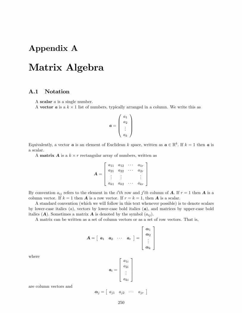
Appendix A
Matrix Algebra
A.1 Notation
A scalar a is a single number.A vector a is a k × 1 list of numbers, typically arranged in a column. We write this as
a =
a1
a2...ak
Equivalently, a vector a is an element of Euclidean k space, written as a ∈ Rk. If k = 1 then a isa scalar.
A matrix A is a k × r rectangular array of numbers, written as
A =
a11 a12 · · · a1r
a21 a22 · · · a2r...
......
ak1 ak2 · · · akr
By convention aij refers to the element in the i′th row and j′th column of A. If r = 1 then A is acolumn vector. If k = 1 then A is a row vector. If r = k = 1, then A is a scalar.
A standard convention (which we will follow in this text whenever possible) is to denote scalarsby lower-case italics (a), vectors by lower-case bold italics (a), and matrices by upper-case bolditalics (A). Sometimes a matrix A is denoted by the symbol (aij).
A matrix can be written as a set of column vectors or as a set of row vectors. That is,
A =[a1 a2 · · · ar
]=
α1
α2...αk
where
ai =
a1i
a2i...aki
are column vectors and
αj =[aj1 aj2 · · · ajr
]250
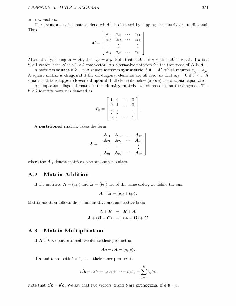
APPENDIX A. MATRIX ALGEBRA 251
are row vectors.The transpose of a matrix, denoted A′, is obtained by flipping the matrix on its diagonal.
Thus
A′ =
a11 a21 · · · ak1
a12 a22 · · · ak2...
......
a1r a2r · · · akr
Alternatively, letting B = A′, then bij = aji. Note that if A is k × r, then A′ is r × k. If a is ak × 1 vector, then a′ is a 1× k row vector. An alternative notation for the transpose of A is A>.
A matrix is square if k = r. A square matrix is symmetric if A = A′, which requires aij = aji.A square matrix is diagonal if the off-diagonal elements are all zero, so that aij = 0 if i 6= j. Asquare matrix is upper (lower) diagonal if all elements below (above) the diagonal equal zero.
An important diagonal matrix is the identity matrix, which has ones on the diagonal. Thek × k identity matrix is denoted as
Ik =
1 0 · · · 00 1 · · · 0......
...0 0 · · · 1
.A partitioned matrix takes the form
A =
A11 A12 · · · A1r
A21 A22 · · · A2r...
......
Ak1 Ak2 · · · Akr
where the Aij denote matrices, vectors and/or scalars.
A.2 Matrix Addition
If the matrices A = (aij) and B = (bij) are of the same order, we define the sum
A+B = (aij + bij) .
Matrix addition follows the communtative and associative laws:
A+B = B +A
A+ (B +C) = (A+B) +C.
A.3 Matrix Multiplication
If A is k × r and c is real, we define their product as
Ac = cA = (aijc) .
If a and b are both k × 1, then their inner product is
a′b = a1b1 + a2b2 + · · ·+ akbk =k∑j=1
ajbj .
Note that a′b = b′a. We say that two vectors a and b are orthogonal if a′b = 0.
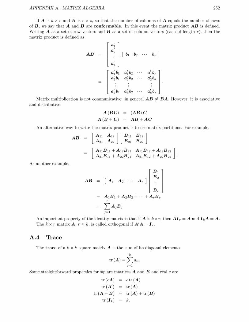
APPENDIX A. MATRIX ALGEBRA 252
If A is k × r and B is r × s, so that the number of columns of A equals the number of rowsof B, we say that A and B are conformable. In this event the matrix product AB is defined.Writing A as a set of row vectors and B as a set of column vectors (each of length r), then thematrix product is defined as
AB =
a′1a′2...a′k
[ b1 b2 · · · bs]
=
a′1b1 a′1b2 · · · a′1bsa′2b1 a′2b2 · · · a′2bs...
......
a′kb1 a′kb2 · · · a′kbs
.Matrix multiplication is not communicative: in general AB 6= BA. However, it is associative
and distributive:
A (BC) = (AB)C
A (B +C) = AB +AC
An alternative way to write the matrix product is to use matrix partitions. For example,
AB =
[A11 A12
A21 A22
] [B11 B12
B21 B22
]
=
[A11B11 +A12B21 A11B12 +A12B22
A21B11 +A22B21 A21B12 +A22B22
].
As another example,
AB =[A1 A2 · · · Ar
]B1
B2...Br
= A1B1 +A2B2 + · · ·+ArBr
=r∑j=1
AjBj
An important property of the identity matrix is that if A is k×r, then AIr = A and IkA = A.The k × r matrix A, r ≤ k, is called orthogonal if A′A = Ir.
A.4 Trace
The trace of a k × k square matrix A is the sum of its diagonal elements
tr (A) =
k∑i=1
aii.
Some straightforward properties for square matrices A and B and real c are
tr (cA) = c tr (A)
tr(A′)
= tr (A)
tr (A+B) = tr (A) + tr (B)
tr (Ik) = k.
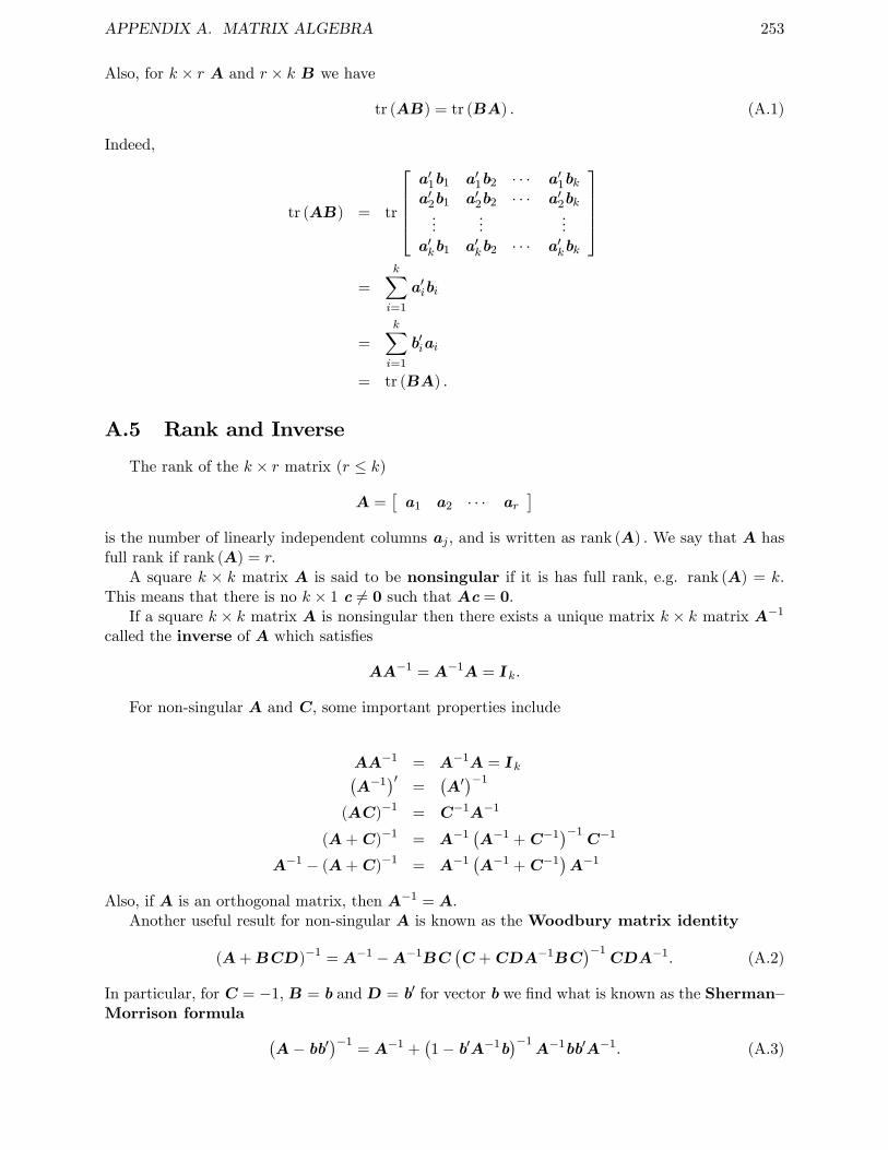
APPENDIX A. MATRIX ALGEBRA 253
Also, for k × r A and r × k B we have
tr (AB) = tr (BA) . (A.1)
Indeed,
tr (AB) = tr
a′1b1 a′1b2 · · · a′1bka′2b1 a′2b2 · · · a′2bk...
......
a′kb1 a′kb2 · · · a′kbk
=
k∑i=1
a′ibi
=k∑i=1
b′iai
= tr (BA) .
A.5 Rank and Inverse
The rank of the k × r matrix (r ≤ k)
A =[a1 a2 · · · ar
]is the number of linearly independent columns aj , and is written as rank (A) . We say that A hasfull rank if rank (A) = r.
A square k × k matrix A is said to be nonsingular if it is has full rank, e.g. rank (A) = k.This means that there is no k × 1 c 6= 0 such that Ac = 0.
If a square k × k matrix A is nonsingular then there exists a unique matrix k × k matrix A−1
called the inverse of A which satisfies
AA−1 = A−1A = Ik.
For non-singular A and C, some important properties include
AA−1 = A−1A = Ik(A−1
)′=
(A′)−1
(AC)−1 = C−1A−1
(A+C)−1 = A−1(A−1 +C−1
)−1C−1
A−1 − (A+C)−1 = A−1(A−1 +C−1
)A−1
Also, if A is an orthogonal matrix, then A−1 = A.Another useful result for non-singular A is known as theWoodbury matrix identity
(A+BCD)−1 = A−1 −A−1BC(C +CDA−1BC
)−1CDA−1. (A.2)
In particular, for C = −1, B = b and D = b′ for vector b we find what is known as the Sherman—Morrison formula (
A− bb′)−1
= A−1 +(1− b′A−1b
)−1A−1bb′A−1. (A.3)
APPENDIX A. MATRIX ALGEBRA 254
The following fact about inverting partitioned matrices is quite useful.[A11 A12
A21 A22
]−1
=
[A11 A12
A21 A22
]=
[A−1
11·2 −A−111·2A21A
−122
−A−122·1A21A
−111 A−1
22·1
](A.4)
where A11·2 = A11 −A12A−122 A21 and A22·1 = A22 −A21A
−111 A12. There are alternative algebraic
representations for the components. For example, using the Woodbury matrix identity you canshow the following alternative expressions
A11 = A−111 +A−1
11 A12A−122·1A21A
−111
A22 = A−122 +A−1
22 A21A−111·2A12A
−122
A12 = −A−111 A21A
−122·1
A21 = −A−122 A21A
−1112
Even if a matrix A does not possess an inverse, we can still define the Moore-Penrose gen-eralized inverse A− as the matrix which satisfies
AA−A = A
A−AA− = A−
AA− is symmetric
A−A is symmetric
For any matrix A, the Moore-Penrose generalized inverse A− exists and is unique.For example, if
A =
[A11 00 0
]then
A− =
[A−11 00 0
].
A.6 Determinant
The determinant is a measure of the volume of a square matrix.While the determinant is widely used, its precise definition is rarely needed. However, we present
the definition here for completeness. Let A = (aij) be a general k × k matrix . Let π = (j1, ..., jk)denote a permutation of (1, ..., k) . There are k! such permutations. There is a unique count of thenumber of inversions of the indices of such permutations (relative to the natural order (1, ..., k) ,and let επ = +1 if this count is even and επ = −1 if the count is odd. Then the determinant of Ais defined as
detA =∑π
επa1j1a2j2 · · · akjk .
For example, if A is 2 × 2, then the two permutations of (1, 2) are (1, 2) and (2, 1) , for whichε(1,2) = 1 and ε(2,1) = −1. Thus
detA = ε(1,2)a11a22 + ε(2,1)a21a12
= a11a22 − a12a21.
Some properties include
• det (A) = det (A′)
• det (cA) = ck detA
APPENDIX A. MATRIX ALGEBRA 255
• det (AB) = (detA) (detB)
• det(A−1
)= (detA)−1
• det
[A BC D
]= (detD) det
(A−BD−1C
)if detD 6= 0
• detA 6= 0 if and only if A is nonsingular.
• If A is triangular (upper or lower), then detA =∏ki=1 aii
• If A is orthogonal, then detA = ±1
A.7 Eigenvalues
The characteristic equation of a square matrix A is
det (A− λIk) = 0.
The left side is a polynomial of degree k in λ so it has exactly k roots, which are not necessarilydistinct and may be real or complex. They are called the latent roots or characteristic roots oreigenvalues of A. If λi is an eigenvalue of A, then A− λiIk is singular so there exists a non-zerovector hi such that
(A− λiIk)hi = 0.
The vector hi is called a latent vector or characteristic vector or eigenvector of A corre-sponding to λi.
We now state some useful properties. Let λi and hi, i = 1, ..., k denote the k eigenvalues andeigenvectors of a square matrix A. Let Λ be a diagonal matrix with the characteristic roots in thediagonal, and let H = [h1 · · ·hk].
• det(A) =∏ki=1 λi
• tr(A) =∑k
i=1 λi
• A is non-singular if and only if all its characteristic roots are non-zero.
• If A has distinct characteristic roots, there exists a nonsingular matrix P such that A =P−1ΛP and PAP−1 = Λ.
• If A is symmetric, then A = HΛH ′ and H ′AH = Λ, and the characteristic roots are allreal. A = HΛH ′ is called the spectral decomposition of a matrix.
• The characteristic roots of A−1 are λ−11 , λ−1
2 , ..., λ−1k .
• The matrix H has the orthonormal properties H ′H = I and HH ′ = I.
• H−1 = H ′ and (H ′)−1= H
A.8 Positive Definiteness
We say that a k × k symmetric square matrix A is positive semi-definite if for all c 6= 0,c′Ac ≥ 0. This is written as A ≥ 0. We say that A is positive definite if for all c 6= 0, c′Ac > 0.This is written as A > 0.
Some properties include:
APPENDIX A. MATRIX ALGEBRA 256
• If A = G′G for some matrix G, then A is positive semi-definite. (For any c 6= 0, c′Ac =α′α ≥ 0 where α = Gc.) If G has full rank, then A is positive definite.
• If A is positive definite, then A is non-singular and A−1 exists. Furthermore, A−1 > 0.
• A > 0 if and only if it is symmetric and all its characteristic roots are positive.
• By the spectral decomposition, A = HΛH ′ where H ′H = I and Λ is diagonal with non-negative diagonal elements. All diagonal elements of Λ are strictly positive if (and only if)A > 0.
• If A > 0 then A−1 = HΛ−1H ′.
• If A ≥ 0 and rank (A) = r < k then A− = HΛ−H ′ where A− is the Moore-Penrosegeneralized inverse, and Λ− = diag
(λ−1
1 , λ−12 , ..., λ−1
k , 0, ..., 0)
• If A > 0 we can find a matrix B such that A = BB′. We call B a matrix square rootof A. The matrix B need not be unique. One way to construct B is to use the spectraldecomposition A = HΛH ′ where Λ is diagonal, and then set B = HΛ1/2.
A square matrix A is idempotent if AA = A. If A is idempotent and symmetric then all itscharacteristic roots equal either zero or one and is thus positive semi-definite. To see this, notethat we can write A = HΛH ′ where H is orthogonal and Λ contains the r (real) characteristicroots. Then
A = AA = HΛH ′HΛH ′ = HΛ2H ′.
By the uniqueness of the characteristic roots, we deduce that Λ2 = Λ and λ2i = λi for i = 1, ..., r.
Hence they must equal either 0 or 1. It follows that the spectral decomposition of idempotent Atakes the form
A = H
[Ik−r 0
0 0
]H ′ (A.5)
with H ′H = Ik. Additionally, tr(A) = rank(A).
A.9 Matrix Calculus
Let x = (x1, ..., xk) be k × 1 and g(x) = g(x1, ..., xk) : Rk → R. The vector derivative is
∂
∂xg (x) =
∂∂x1
g (x)...
∂∂xk
g (x)
and
∂
∂x′g (x) =
(∂∂x1
g (x) · · · ∂∂xk
g (x)).
Some properties are now summarized.
• ∂∂x (a′x) = ∂
∂x (x′a) = a
• ∂∂x′ (Ax) = A
• ∂∂x (x′Ax) = (A+A′)x
• ∂2
∂x∂x′ (x′Ax) = A+A′
APPENDIX A. MATRIX ALGEBRA 257
A.10 Kronecker Products and the Vec Operator
Let A = [a1 a2 · · · an] be m× n. The vec of A, denoted by vec (A) , is the mn× 1 vector
vec (A) =
a1
a2...an
.
Let A = (aij) be an m × n matrix and let B be any matrix. The Kronecker product of Aand B, denoted A⊗B, is the matrix
A⊗B =
a11B a12B a1nBa21B a22B · · · a2nB...
......
am1B am2B · · · amnB
.Some important properties are now summarized. These results hold for matrices for which allmatrix multiplications are conformable.
• (A+B)⊗C = A⊗C +B ⊗C
• (A⊗B) (C ⊗D) = AC ⊗BD
• A⊗ (B ⊗C) = (A⊗B)⊗ C
• (A⊗B)′ = A′ ⊗B′
• tr (A⊗B) = tr (A) tr (B)
• If A is m×m and B is n× n, det(A⊗B) = (det (A))n (det (B))m
• (A⊗B)−1 = A−1 ⊗B−1
• If A > 0 and B > 0 then A⊗B > 0
• vec (ABC) = (C ′ ⊗A) vec (B)
• tr (ABCD) = vec (D′)′ (C ′ ⊗A) vec (B)
A.11 Vector and Matrix Norms and Inequalities
The Euclidean norm of an m× 1 vector a is
‖a‖ =(a′a)1/2
=
(m∑i=1
a2i
)1/2
.
The Euclidean norm of an m× n matrix A is
‖A‖ = ‖vec (A)‖= tr
(A′A
)1/2=
m∑i=1
n∑j=1
a2ij
1/2
.
APPENDIX A. MATRIX ALGEBRA 258
A useful calculation is for any m× 1 vectors a and b, using (A.1),∥∥ab′∥∥ = tr(ba′ab
′)1/2
=(b′ba′a
)1/2= ‖a‖ ‖b‖
and in particular ∥∥aa′∥∥ = ‖a‖2 (A.6)
Some useful inequalities are now given:
Schwarz Inequality: For any m× 1 vectors a and b,∣∣a′b∣∣ ≤ ‖a‖ ‖b‖ . (A.7)
Schwarz Matrix Inequality: For any m× n matrices A and B,∥∥A′B∥∥ ≤ ‖A‖ ‖B‖ . (A.8)
Triangle Inequality: For any m× n matrices A and B,
‖A+B‖ ≤ ‖A‖+ ‖B‖ . (A.9)
Trace Inequality. For any m×m matrices A and B such that A is symmetric and B ≥ 0
tr (AB) ≤ λmax (A) tr (B) (A.10)
where λmax (A) is the largest eigenvalue of A.
Proof of Schwarz Inequality: First, suppose that ‖b‖ = 0. Then b = 0 and both |a′b| = 0 and‖a‖ ‖b‖ = 0 so the inequality is true. Second, suppose that ‖b‖ > 0 and define c = a−b
(b′b)−1
b′a.Since c is a vector, c′c ≥ 0. Thus
0 ≤ c′c = a′a−(a′b)2/(b′b).
Rearranging, this implies that (a′b)2 ≤ (a′a) (b′b) .
Taking the square root of each side yields the result.
Proof of Schwarz Matrix Inequality: Partition A = [a1, ...,an] and B = [b1, ..., bn]. Thenby partitioned matrix multiplication, the definition of the matrix Euclidean norm and the Schwarzinequality
∥∥A′B∥∥ =
∥∥∥∥∥∥∥a′1b1 a′1b2 · · ·a′2b1 a′2b2 · · ·...
.... . .
∥∥∥∥∥∥∥≤
∥∥∥∥∥∥∥‖a1‖ ‖b1‖ ‖a1‖ ‖b2‖ · · ·‖a2‖ ‖b1‖ ‖a2‖ ‖b2‖ · · ·
......
. . .
∥∥∥∥∥∥∥=
n∑i=1
n∑j=1
‖ai‖2 ‖bj‖21/2
=
(n∑i=1
‖ai‖2)1/2( n∑
i=1
‖bi‖2)1/2
=
n∑i=1
m∑j=1
a2ji
1/2 n∑i=1
m∑j=1
‖bji‖21/2
= ‖A‖ ‖B‖
APPENDIX A. MATRIX ALGEBRA 259
Proof of Triangle Inequality: Let a = vec (A) and b = vec (B) . Then by the definition of thematrix norm and the Schwarz Inequality
‖A+B‖2 = ‖a+ b‖2
= a′a+ 2a′b+ b′b
≤ a′a+ 2∣∣a′b∣∣+ b′b
≤ ‖a‖2 + 2 ‖a‖ ‖b‖+ ‖b‖2
= (‖a‖+ ‖b‖)2
= (‖A‖+ ‖B‖)2
Proof of Trace Inequality. By the spectral decomposition for symmetric matices, A =HΛH ′ where Λ has the eigenvalues λj of A on the diagonal and H is orthonormal. DefineC = H ′BH which has non-negative diagonal elements Cjj since B is positive semi-definite. Then
tr (AB) = tr (ΛC) =
m∑j=1
λjCjj ≤ maxjλj
m∑j=1
Cjj = λmax (A) tr (C)
where the inequality uses the fact that Cjj ≥ 0. But note that
tr (C) = tr(H ′BH
)= tr
(HH ′B
)= tr (B)
since H is orthonormal. Thus tr (AB) ≤ λmax (A) tr (B) as stated.
Appendix B
Probability
B.1 Foundations
The set S of all possible outcomes of an experiment is called the sample space for the exper-iment. Take the simple example of tossing a coin. There are two outcomes, heads and tails, sowe can write S = H,T. If two coins are tossed in sequence, we can write the four outcomes asS = HH,HT, TH, TT.
An event A is any collection of possible outcomes of an experiment. An event is a subset of S,including S itself and the null set ∅. Continuing the two coin example, one event is A = HH,HT,the event that the first coin is heads. We say that A and B are disjoint or mutually exclusiveif A ∩ B = ∅. For example, the sets HH,HT and TH are disjoint. Furthermore, if the setsA1, A2, ... are pairwise disjoint and ∪∞i=1Ai = S, then the collection A1, A2, ... is called a partitionof S.
The following are elementary set operations:Union: A ∪B = x : x ∈ A or x ∈ B.Intersection: A ∩B = x : x ∈ A and x ∈ B.Complement: Ac = x : x /∈ A.The following are useful properties of set operations.Communtatitivity: A ∪B = B ∪A; A ∩B = B ∩A.Associativity: A ∪ (B ∪ C) = (A ∪B) ∪ C; A ∩ (B ∩ C) = (A ∩B) ∩ C.Distributive Laws: A∩ (B ∪ C) = (A ∩B)∪ (A ∩ C) ; A∪ (B ∩ C) = (A ∪B)∩ (A ∪ C) .DeMorgan’s Laws: (A ∪B)c = Ac ∩Bc; (A ∩B)c = Ac ∪Bc.A probability function assigns probabilities (numbers between 0 and 1) to events A in S.
This is straightforward when S is countable; when S is uncountable we must be somewhat morecareful. A set B is called a sigma algebra (or Borel field) if ∅ ∈ B , A ∈ B implies Ac ∈ B, andA1, A2, ... ∈ B implies ∪∞i=1Ai ∈ B. A simple example is ∅, S which is known as the trivial sigmaalgebra. For any sample space S, let B be the smallest sigma algebra which contains all of the opensets in S. When S is countable, B is simply the collection of all subsets of S, including ∅ and S.When S is the real line, then B is the collection of all open and closed intervals. We call B thesigma algebra associated with S. We only define probabilities for events contained in B.
We now can give the axiomatic definition of probability. Given S and B, a probability functionPr satisfies Pr(S) = 1, Pr(A) ≥ 0 for all A ∈ B, and if A1, A2, ... ∈ B are pairwise disjoint, thenPr (∪∞i=1Ai) =
∑∞i=1 Pr(Ai).
Some important properties of the probability function include the following
• Pr (∅) = 0
• Pr(A) ≤ 1
• Pr (Ac) = 1− Pr(A)
260
APPENDIX B. PROBABILITY 261
• Pr (B ∩Ac) = Pr(B)− Pr(A ∩B)
• Pr (A ∪B) = Pr(A) + Pr(B)− Pr(A ∩B)
• If A ⊂ B then Pr(A) ≤ Pr(B)
• Bonferroni’s Inequality: Pr(A ∩B) ≥ Pr(A) + Pr(B)− 1
• Boole’s Inequality: Pr (A ∪B) ≤ Pr(A) + Pr(B)
For some elementary probability models, it is useful to have simple rules to count the numberof objects in a set. These counting rules are facilitated by using the binomial coeffi cients which aredefined for nonnegative integers n and r, n ≥ r, as(
n
r
)=
n!
r! (n− r)! .
When counting the number of objects in a set, there are two important distinctions. Countingmay be with replacement or without replacement. Counting may be ordered or unordered.For example, consider a lottery where you pick six numbers from the set 1, 2, ..., 49. This selection iswithout replacement if you are not allowed to select the same number twice, and is with replacementif this is allowed. Counting is ordered or not depending on whether the sequential order of thenumbers is relevant to winning the lottery. Depending on these two distinctions, we have fourexpressions for the number of objects (possible arrangements) of size r from n objects.
Without WithReplacement Replacement
Ordered n!(n−r)! nr
Unordered(nr
) (n+r−1
r
)In the lottery example, if counting is unordered and without replacement, the number of po-
tential combinations is(
496
)= 13, 983, 816.
If Pr(B) > 0 the conditional probability of the event A given the event B is
Pr (A | B) =Pr (A ∩B)
Pr(B).
For any B, the conditional probability function is a valid probability function where S has beenreplaced by B. Rearranging the definition, we can write
Pr(A ∩B) = Pr (A | B) Pr(B)
which is often quite useful. We can say that the occurrence of B has no information about thelikelihood of event A when Pr (A | B) = Pr(A), in which case we find
Pr(A ∩B) = Pr (A) Pr(B) (B.1)
We say that the events A and B are statistically independent when (B.1) holds. Furthermore,we say that the collection of events A1, ..., Ak are mutually independent when for any subsetAi : i ∈ I,
Pr
(⋂i∈I
Ai
)=∏i∈I
Pr (Ai) .
Theorem 1 (Bayes’Rule). For any set B and any partition A1, A2, ... of the sample space, thenfor each i = 1, 2, ...
Pr (Ai | B) =Pr (B | Ai) Pr(Ai)∑∞j=1 Pr (B | Aj) Pr(Aj)
APPENDIX B. PROBABILITY 262
B.2 Random Variables
A random variable X is a function from a sample space S into the real line. This induces anew sample space —the real line —and a new probability function on the real line. Typically, wedenote random variables by uppercase letters such as X, and use lower case letters such as x forpotential values and realized values. (This is in contrast to the notation adopted for most of thetextbook.) For a random variable X we define its cumulative distribution function (CDF) as
F (x) = Pr (X ≤ x) . (B.2)
Sometimes we write this as FX(x) to denote that it is the CDF of X. A function F (x) is a CDF ifand only if the following three properties hold:
1. limx→−∞ F (x) = 0 and limx→∞ F (x) = 1
2. F (x) is nondecreasing in x
3. F (x) is right-continuous
We say that the random variable X is discrete if F (x) is a step function. In the latter case,the range of X consists of a countable set of real numbers τ1, ..., τ r. The probability function forX takes the form
Pr (X = τ j) = πj , j = 1, ..., r (B.3)
where 0 ≤ πj ≤ 1 and∑r
j=1 πj = 1.We say that the random variableX is continuous if F (x) is continuous in x. In this case Pr(X =
τ) = 0 for all τ ∈ R so the representation (B.3) is unavailable. Instead, we represent the relativeprobabilities by the probability density function (PDF)
f(x) =d
dxF (x)
so that
F (x) =
∫ x
−∞f(u)du
and
Pr (a ≤ X ≤ b) =
∫ b
af(u)du.
These expressions only make sense if F (x) is differentiable. While there are examples of continuousrandom variables which do not possess a PDF, these cases are unusual and are typically ignored.
A function f(x) is a PDF if and only if f(x) ≥ 0 for all x ∈ R and∫∞−∞ f(x)dx.
B.3 Expectation
For any measurable real function g, we define the mean or expectation Eg(X) as follows. IfX is discrete,
Eg(X) =r∑j=1
g(τ j)πj ,
and if X is continuous
Eg(X) =
∫ ∞−∞
g(x)f(x)dx.
The latter is well defined and finite if∫ ∞−∞|g(x)| f(x)dx <∞. (B.4)
APPENDIX B. PROBABILITY 263
If (B.4) does not hold, evaluate
I1 =
∫g(x)>0
g(x)f(x)dx
I2 = −∫g(x)<0
g(x)f(x)dx
If I1 = ∞ and I2 < ∞ then we define Eg(X) = ∞. If I1 < ∞ and I2 = ∞ then we defineEg(X) = −∞. If both I1 =∞ and I2 =∞ then Eg(X) is undefined.
Since E (a+ bX) = a+ bEX, we say that expectation is a linear operator.For m > 0, we define the m′th moment of X as EXm and the m′th central moment as
E (X − EX)m .Two special moments are the mean µ = EX and variance σ2 = E (X − µ)2 = EX2 − µ2. We
call σ =√σ2 the standard deviation of X. We can also write σ2 = var(X). For example, this
allows the convenient expression var(a+ bX) = b2 var(X).The moment generating function (MGF) of X is
M(λ) = E exp (λX) .
The MGF does not necessarily exist. However, when it does and E |X|m <∞ then
dm
dλmM(λ)
∣∣∣∣λ=0
= E (Xm)
which is why it is called the moment generating function.More generally, the characteristic function (CF) of X is
C(λ) = E exp (iλX)
where i =√−1 is the imaginary unit. The CF always exists, and when E |X|m <∞
dm
dλmC(λ)
∣∣∣∣λ=0
= imE (Xm) .
The Lp norm, p ≥ 1, of the random variable X is
‖X‖p = (E |X|p)1/p .
B.4 Gamma Function
The gamma function is defined for α > 0 as
Γ(α) =
∫ ∞0
xα−1 exp (−x) .
It satisfies the propertyΓ(1 + α) = Γ(α)α
so for positive integers n,Γ(n) = (n− 1)!
Special values includeΓ (1) = 1
and
Γ
(1
2
)= π1/2.
Sterling’s formula is an expansion for the its logarithm
log Γ(α) =1
2log(2π) +
(α− 1
2
)logα− z +
1
12α− 1
360α3+
1
1260α5+ · · ·
APPENDIX B. PROBABILITY 264
B.5 Common Distributions
For reference, we now list some important discrete distribution function.Bernoulli
Pr (X = x) = px(1− p)1−x, x = 0, 1; 0 ≤ p ≤ 1
EX = p
var(X) = p(1− p)
Binomial
Pr (X = x) =
(n
x
)px (1− p)n−x , x = 0, 1, ..., n; 0 ≤ p ≤ 1
EX = np
var(X) = np(1− p)
Geometric
Pr (X = x) = p(1− p)x−1, x = 1, 2, ...; 0 ≤ p ≤ 1
EX =1
p
var(X) =1− pp2
Multinomial
Pr (X1 = x1, X2 = x2, ..., Xm = xm) =n!
x1!x2! · · ·xm!px11 p
x22 · · · pxmm ,
x1 + · · ·+ xm = n;
p1 + · · ·+ pm = 1
EXi = pi
var(Xi) = npi(1− pi)cov (Xi, Xj) = −npipj
Negative Binomial
Pr (X = x) =Γ (r + x)
x!Γ (r)pr(1− p)x−1, x = 0, 1, 2, ...; 0 ≤ p ≤ 1
EX =r (1− p)
p
var(X) =r (1− p)
p2
Poisson
Pr (X = x) =exp (−λ)λx
x!, x = 0, 1, 2, ..., λ > 0
EX = λ
var(X) = λ
We now list some important continuous distributions.
APPENDIX B. PROBABILITY 265
Beta
f(x) =Γ(α+ β)
Γ(α)Γ(β)xα−1(1− x)β−1, 0 ≤ x ≤ 1; α > 0, β > 0
µ =α
α+ β
var(X) =αβ
(α+ β + 1) (α+ β)2
Cauchy
f(x) =1
π (1 + x2), −∞ < x <∞
EX = ∞var(X) = ∞
Exponential
f(x) =1
θexp
(xθ
), 0 ≤ x <∞; θ > 0
EX = θ
var(X) = θ2
Logistic
f(x) =exp (−x)
(1 + exp (−x))2 , −∞ < x <∞;
EX = 0
var(X) =π2
3
Lognormal
f(x) =1√
2πσxexp
(−(log x− µ)2
2σ2
), 0 ≤ x <∞; σ > 0
EX = exp(µ+ σ2/2
)var(X) = exp
(2µ+ 2σ2
)− exp
(2µ+ σ2
)Pareto
f(x) =βαβ
xβ+1, α ≤ x <∞, α > 0, β > 0
EX =βα
β − 1, β > 1
var(X) =βα2
(β − 1)2 (β − 2), β > 2
Uniform
f(x) =1
b− a, a ≤ x ≤ b
EX =a+ b
2
var(X) =(b− a)2
12
APPENDIX B. PROBABILITY 266
Weibull
f(x) =γ
βxγ−1 exp
(−x
γ
β
), 0 ≤ x <∞; γ > 0, β > 0
EX = β1/γΓ
(1 +
1
γ
)var(X) = β2/γ
(Γ
(1 +
2
γ
)− Γ2
(1 +
1
γ
))Gamma
f(x) =1
Γ(α)θαxα−1 exp
(−xθ
), 0 ≤ x <∞; α > 0, θ > 0
EX = αθ
var(X) = αθ2
Chi-Square
f(x) =1
Γ(r/2)2r/2xr/2−1 exp
(−x
2
), 0 ≤ x <∞; r > 0
EX = r
var(X) = 2r
Normal
f(x) =1√2πσ
exp
(−(x− µ)2
2σ2
), −∞ < x <∞; −∞ < µ <∞, σ2 > 0
EX = µ
var(X) = σ2
Student t
f(x) =Γ(r+1
2
)√rπΓ
(r2
) (1 +x2
r
)−( r+12 ), −∞ < x <∞; r > 0
EX = 0 if r > 1
var(X) =r
r − 2if r > 2
B.6 Multivariate Random Variables
A pair of bivariate random variables (X,Y ) is a function from the sample space into R2. Thejoint CDF of (X,Y ) is
F (x, y) = Pr (X ≤ x, Y ≤ y) .
If F is continuous, the joint probability density function is
f(x, y) =∂2
∂x∂yF (x, y).
For a Borel measurable set A ∈ R2,
Pr ((X < Y ) ∈ A) =
∫ ∫Af(x, y)dxdy
APPENDIX B. PROBABILITY 267
For any measurable function g(x, y),
Eg(X,Y ) =
∫ ∞−∞
∫ ∞−∞
g(x, y)f(x, y)dxdy.
The marginal distribution of X is
FX(x) = Pr(X ≤ x)
= limy→∞
F (x, y)
=
∫ x
−∞
∫ ∞−∞
f(x, y)dydx
so the marginal density of X is
fX(x) =d
dxFX(x) =
∫ ∞−∞
f(x, y)dy.
Similarly, the marginal density of Y is
fY (y) =
∫ ∞−∞
f(x, y)dx.
The random variables X and Y are defined to be independent if f(x, y) = fX(x)fY (y).Furthermore, X and Y are independent if and only if there exist functions g(x) and h(y) such thatf(x, y) = g(x)h(y).
If X and Y are independent, then
E (g(X)h(Y )) =
∫ ∫g(x)h(y)f(y, x)dydx
=
∫ ∫g(x)h(y)fY (y)fX(x)dydx
=
∫g(x)fX(x)dx
∫h(y)fY (y)dy
= Eg (X)Eh (Y ) . (B.5)
if the expectations exist. For example, if X and Y are independent then
E(XY ) = EXEY.
Another implication of (B.5) is that if X and Y are independent and Z = X + Y, then
MZ(λ) = E exp (λ (X + Y ))
= E (exp (λX) exp (λY ))
= E exp(λ′X
)E exp
(λ′Y
)= MX(λ)MY (λ). (B.6)
The covariance between X and Y is
cov(X,Y ) = σXY = E ((X − EX) (Y − EY )) = EXY − EXEY.
The correlation between X and Y is
corr (X,Y ) = ρXY =σXYσxσY
.
APPENDIX B. PROBABILITY 268
The Cauchy-Schwarz Inequality implies that
|ρXY | ≤ 1. (B.7)
The correlation is a measure of linear dependence, free of units of measurement.If X and Y are independent, then σXY = 0 and ρXY = 0. The reverse, however, is not true.
For example, if EX = 0 and EX3 = 0, then cov(X,X2) = 0.A useful fact is that
var (X + Y ) = var(X) + var(Y ) + 2 cov(X,Y ).
An implication is that if X and Y are independent, then
var (X + Y ) = var(X) + var(Y ),
the variance of the sum is the sum of the variances.A k×1 random vectorX = (X1, ..., Xk)
′ is a function from S to Rk. Let x = (x1, ..., xk)′ denote
a vector in Rk. (In this Appendix, we use bold to denote vectors. Bold capitals X are randomvectors and bold lower case x are nonrandom vectors. Again, this is in distinction to the notationused in the bulk of the text) The vector X has the distribution and density functions
F (x) = Pr(X ≤ x)
f(x) =∂k
∂x1 · · · ∂xkF (x).
For a measurable function g : Rk → Rs, we define the expectation
Eg(X) =
∫Rkg(x)f(x)dx
where the symbol dx denotes dx1 · · · dxk. In particular, we have the k × 1 multivariate mean
µ = EX
and k × k covariance matrix
Σ = E((X − µ) (X − µ)′
)= EXX ′ − µµ′
If the elements of X are mutually independent, then Σ is a diagonal matrix and
var
(k∑i=1
Xi
)=
k∑i=1
var (Xi)
B.7 Conditional Distributions and Expectation
The conditional density of Y given X = x is defined as
fY |X (y | x) =f(x, y)
fX(x)
APPENDIX B. PROBABILITY 269
if fX(x) > 0. One way to derive this expression from the definition of conditional probability is
fY |X (y | x) =∂
∂ylimε→0
Pr (Y ≤ y | x ≤X ≤ x+ ε)
=∂
∂ylimε→0
Pr (Y ≤ y ∩ x ≤X ≤ x+ ε)Pr(x ≤ X ≤ x+ ε)
=∂
∂ylimε→0
F (x+ ε, y)− F (x, y)
FX(x+ ε)− FX(x)
=∂
∂ylimε→0
∂∂xF (x+ ε, y)
fX(x+ ε)
=
∂2
∂x∂yF (x, y)
fX(x)
=f(x, y)
fX(x).
The conditional mean or conditional expectation is the function
m(x) = E (Y |X = x) =
∫ ∞−∞
yfY |X (y | x) dy.
The conditional mean m(x) is a function, meaning that when X equals x, then the expected valueof Y is m(x).
Similarly, we define the conditional variance of Y given X = x as
σ2(x) = var (Y |X = x)
= E(
(Y −m(x))2 |X = x)
= E(Y 2 | X = x
)−m(x)2.
Evaluated at x = X, the conditional mean m(X) and conditional variance σ2(X) are randomvariables, functions of X. We write this as E(Y | X) = m(X) and var (Y |X) = σ2(X). Forexample, if E (Y |X = x) = α+ β′x, then E (Y |X) = α+ β′X, a transformation of X.
The following are important facts about conditional expectations.Simple Law of Iterated Expectations:
E (E (Y |X)) = E (Y ) (B.8)
Proof :
E (E (Y |X)) = E (m(X))
=
∫ ∞−∞
m(x)fX(x)dx
=
∫ ∞−∞
∫ ∞−∞
yfY |X (y | x) fX(x)dydx
=
∫ ∞−∞
∫ ∞−∞
yf (y,x) dydx
= E(Y ).
Law of Iterated Expectations:
E (E (Y |X,Z) |X) = E (Y |X) (B.9)
APPENDIX B. PROBABILITY 270
Conditioning Theorem. For any function g(x),
E (g(X)Y |X) = g (X)E (Y |X) (B.10)
Proof : Let
h(x) = E (g(X)Y |X = x)
=
∫ ∞−∞
g(x)yfY |X (y | x) dy
= g(x)
∫ ∞−∞
yfY |X (y | x) dy
= g(x)m(x)
where m(x) = E (Y |X = x) . Thus h(X) = g(X)m(X), which is the same as E (g(X)Y |X) =g (X)E (Y |X) .
B.8 Transformations
Suppose that X ∈ Rk with continuous distribution function FX(x) and density fX(x). LetY = g(X) where g(x) : Rk → Rk is one-to-one, differentiable, and invertible. Let h(y) denote theinverse of g(x). The Jacobian is
J(y) = det
(∂
∂y′h(y)
).
Consider the univariate case k = 1. If g(x) is an increasing function, then g(X) ≤ Y if and onlyif X ≤ h(Y ), so the distribution function of Y is
FY (y) = Pr (g(X) ≤ y)
= Pr (X ≤ h(Y ))
= FX (h(Y )) .
Taking the derivative, the density of Y is
fY (y) =d
dyFY (y) = fX (h(Y ))
d
dyh(y).
If g(x) is a decreasing function, then g(X) ≤ Y if and only if X ≥ h(Y ), so
FY (y) = Pr (g(X) ≤ y)
= 1− Pr (X ≥ h(Y ))
= 1− FX (h(Y ))
and the density of Y is
fY (y) = −fX (h(Y ))d
dyh(y).
We can write these two cases jointly as
fY (y) = fX (h(Y )) |J(y)| . (B.11)
This is known as the change-of-variables formula. This same formula (B.11) holds for k > 1, butits justification requires deeper results from analysis.
As one example, take the case X ∼ U [0, 1] and Y = − log(X). Here, g(x) = − log(x) andh(y) = exp(−y) so the Jacobian is J(y) = − exp(y). As the range of X is [0, 1], that for Y is [0,∞).Since fX (x) = 1 for 0 ≤ x ≤ 1 (B.11) shows that
fY (y) = exp(−y), 0 ≤ y ≤ ∞,
an exponential density.
APPENDIX B. PROBABILITY 271
B.9 Normal and Related Distributions
The standard normal density is
φ(x) =1√2π
exp
(−x
2
2
), −∞ < x <∞.
It is conventional to write X ∼ N (0, 1) , and to denote the standard normal density function byφ(x) and its distribution function by Φ(x). The latter has no closed-form solution. The normaldensity has all moments finite. Since it is symmetric about zero all odd moments are zero. Byiterated integration by parts, we can also show that EX2 = 1 and EX4 = 3. In fact, for any positiveinteger m, EX2m = (2m− 1)!! = (2m− 1) · (2m− 3) · · · 1. Thus EX4 = 3, EX6 = 15, EX8 = 105,and EX10 = 945.
If Z is standard normal and X = µ + σZ, then using the change-of-variables formula, X hasdensity
f(x) =1√2πσ
exp
(−(x− µ)2
2σ2
), −∞ < x <∞.
which is the univariate normal density. The mean and variance of the distribution are µ andσ2, and it is conventional to write X ∼ N
(µ, σ2
).
For x ∈ Rk, the multivariate normal density is
f(x) =1
(2π)k/2 det (Σ)1/2exp
(−(x− µ)′Σ−1 (x− µ)
2
), x ∈ Rk.
The mean and covariance matrix of the distribution are µ and Σ, and it is conventional to writeX ∼ N (µ,Σ).
The MGF and CF of the multivariate normal are exp(λ′µ+ λ′Σλ/2
)and exp
(iλ′µ− λ′Σλ/2
),
respectively.If X ∈ Rk is multivariate normal and the elements of X are mutually uncorrelated, then
Σ = diagσ2j is a diagonal matrix. In this case the density function can be written as
f(x) =1
(2π)k/2 σ1 · · ·σkexp
(−(
(x1 − µ1)2 /σ21 + · · ·+ (xk − µk)2 /σ2
k
2
))
=
k∏j=1
1
(2π)1/2 σjexp
(−(xj − µj
)22σ2
j
)
which is the product of marginal univariate normal densities. This shows that if X is multivariatenormal with uncorrelated elements, then they are mutually independent.
Theorem B.9.1 If X ∼ N (µ,Σ) and Y = a + BX with B an invertible matrix, then Y ∼N (a+Bµ,BΣB′) .
Theorem B.9.2 Let X ∼ N (0, Ir) . Then Q = X ′X is distributed chi-square with r degrees offreedom, written χ2
r.
Theorem B.9.3 If Z ∼ N (0,A) with A > 0, q × q, then Z ′A−1Z ∼ χ2q .
Theorem B.9.4 Let Z ∼ N (0, 1) and Q ∼ χ2r be independent. Then Tr = Z/
√Q/r is distributed
as student’s t with r degrees of freedom.
APPENDIX B. PROBABILITY 272
Proof of Theorem B.9.1. By the change-of-variables formula, the density of Y = a+BX is
f(y) =1
(2π)k/2 det (ΣY )1/2exp
(−
(y − µY )′Σ−1Y (y − µY )
2
), y ∈ Rk.
where µY = a+Bµ andΣY = BΣB′, where we used the fact that det (BΣB′)1/2= det (Σ)1/2 det (B) .
Proof of Theorem B.9.2. First, suppose a random variable Q is distributed chi-square with rdegrees of freedom. It has the MGF
E exp (tQ) =
∫ ∞0
1
Γ(r2
)2r/2
xr/2−1 exp (tx) exp (−x/2) dy = (1− 2t)−r/2
where the second equality uses the fact that∫∞
0 ya−1 exp (−by) dy = b−aΓ(a), which can be foundby applying change-of-variables to the gamma function. Our goal is to calculate the MGF ofQ = X ′X and show that it equals (1− 2t)−r/2 , which will establish that Q ∼ χ2
r .Note that we can write Q = X ′X =
∑rj=1 Z
2j where the Zj are independent N (0, 1) . The
distribution of each of the Z2j is
Pr(Z2j ≤ y
)= 2 Pr (0 ≤ Zj ≤
√y)
= 2
∫ √y0
1√2π
exp
(−x
2
2
)dx
=
∫ y
0
1
Γ(
12
)21/2
s−1/2 exp(−s
2
)ds
using the change—of-variables s = x2 and the fact Γ(
12
)=√π. Thus the density of Z2
j is
f1(x) =1
Γ(
12
)21/2
x−1/2 exp(−x
2
)which is the χ2
1 and by our above calculation has the MGF of E exp(tZ2
j
)= (1− 2t)−1/2 .
Since the Z2j are mutually independent, (B.6) implies that the MGF of Q =
∑rj=1 Z
2j is[
(1− 2t)−1/2]r
= (1− 2t)−r/2 , which is the MGF of the χ2r density as desired.
Proof of Theorem B.9.3. The fact that A > 0 means that we can write A = CC ′ where C isnon-singular. Then A−1 = C−1′C−1 and
C−1Z ∼ N(0,C−1AC−1′) = N
(0,C−1CC ′C−1′) = N (0, Iq) .
ThusZ ′A−1Z = Z ′C−1′C−1Z =
(C−1Z
)′ (C−1Z
)∼ χ2
q .
Proof of Theorem B.9.4. Using the simple law of iterated expectations, Tr has distribution
APPENDIX B. PROBABILITY 273
function
F (x) = Pr
(Z√Q/r
≤ x)
= E
Z ≤ x
√Q
r
= E
[Pr
(Z ≤ x
√Q
r| Q)]
= EΦ
(x
√Q
r
)
Thus its density is
f (x) = Ed
dxΦ
(x
√Q
r
)
= E
(φ
(x
√Q
r
)√Q
r
)
=
∫ ∞0
(1√2π
exp
(−qx
2
2r
))√q
r
(1
Γ(r2
)2r/2
qr/2−1 exp (−q/2)
)dq
=Γ(r+1
2
)√rπΓ
(r2
) (1 +x2
r
)−( r+12 )
which is that of the student t with r degrees of freedom.
B.10 Inequalities
Jensen’s Inequality (finite form). If g(·) : R→ R is convex, then for any non-negative weightsaj such that
∑mj=1 aj = 1, and any real numbers xj
g
m∑j=1
ajxj
≤ m∑j=1
ajg (xj) . (B.12)
In particular, setting aj = 1/m, then
g
1
m
m∑j=1
xj
≤ 1
m
m∑j=1
g (xj) . (B.13)
Loève’s cr Inequality. For r > 0, ∣∣∣∣∣∣m∑j=1
aj
∣∣∣∣∣∣r
≤ crm∑j=1
|aj |r (B.14)
where cr = 1 when r ≤ 1 and cr = mr−1 when r ≥ 1.
Jensen’s Inequality (probabilistic form). If g(·) : Rm → R is convex, then for any random
APPENDIX B. PROBABILITY 274
vector x for which E ‖x‖ <∞ and E |g (x)| <∞,
g(E(x)) ≤ E (g (x)) . (B.15)
Conditional Jensen’s Inequality. If g(·) : Rm → R is convex, then for any random vectors(y,x) for which E ‖y‖ <∞ and E ‖g (y)‖ <∞,
g(E(y | x)) ≤ E (g (y) | x) . (B.16)
Conditional Expectation Inequality. For any r ≥ such that E |y|r <∞, then
E |E(y | x)|r ≤ E |y|r <∞. (B.17)
Expectation Inequality. For any random matrix Y for which E ‖Y ‖ <∞,
‖E(Y )‖ ≤ E ‖Y ‖ . (B.18)
Hölder’s Inequality. If p > 1 and q > 1 and 1p + 1
q = 1, then for any random m× n matrices Xand Y,
E∥∥X ′Y ∥∥ ≤ (E ‖X‖p)1/p (E ‖Y ‖q)1/q . (B.19)
Cauchy-Schwarz Inequality. For any random m× n matrices X and Y,
E∥∥X ′Y ∥∥ ≤ (E ‖X‖2)1/2 (
E ‖Y ‖2)1/2
. (B.20)
Matrix Cauchy-Schwarz Inequality. Tripathi (1999). For any random x ∈ Rm and y ∈ R`,
Eyx′(Exx′
)− Exy′ ≤ Eyy′ (B.21)
Minkowski’s Inequality. For any random m× n matrices X and Y,
(E ‖X + Y ‖p)1/p ≤ (E ‖X‖p)1/p + (E ‖Y ‖p)1/p (B.22)
Liapunov’s Inequality. For any random m× n matrix X and 1 ≤ r ≤ p,
(E ‖X‖r)1/r ≤ (E ‖X‖p)1/p (B.23)
Markov’s Inequality (standard form). For any random vector x and non-negative functiong(x) ≥ 0,
Pr(g(x) > α) ≤ α−1Eg(x). (B.24)
Markov’s Inequality (strong form). For any random vector x and non-negative functiong(x) ≥ 0,
Pr(g(x) > α) ≤ α−1E (g (x) 1 (g(x) > α)) . (B.25)
Chebyshev’s Inequality. For any random variable x,
Pr(|x− Ex| > α) ≤ var (x)
α2. (B.26)
APPENDIX B. PROBABILITY 275
Proof of Jensen’s Inequality (B.12). By the definition of convexity, for any λ ∈ [0, 1]
g (λx1 + (1− λ)x2) ≤ λg (x1) + (1− λ) g (x2) . (B.27)
This implies
g
m∑j=1
ajxj
= g
a1g (x1) + (1− a1)
m∑j=2
aj1− a1
xj
≤ a1g (x1) + (1− a1) g
m∑j=2
bjxj
.
where bj = aj/(1− a1) and∑m
j=2 bj = 1. By another application of (B.27) this is bounded by
a1g (x1)+(1− a1)
b2g(x2) + (1− b2)g
m∑j=2
cjxj
= a1g (x1)+a2g(x2)+(1− a1) (1−b2)g
m∑j=2
cjxj
where cj = bj/(1− b2). By repeated application of (B.27) we obtain (B.12).
Proof of Loève’s cr Inequality. For r ≥ 1 this is simply a rewriting of the finite form Jensen’s
inequality (B.13) with g(u) = ur. For r < 1, define bj = |aj | /(∑m
j=1 |aj |). The facts that 0 ≤ bj ≤ 1
and r < 1 imply bj ≤ brj and thus
1 =m∑j=1
bj ≤m∑j=1
brj
which implies m∑j=1
|aj |
r
≤m∑j=1
|aj |r .
The proof is completed by observing that m∑j=1
aj
r
≤
m∑j=1
|aj |
r
.
Proof of Jensen’s Inequality (B.15). Since g(u) is convex, at any point u there is a nonemptyset of subderivatives (linear surfaces touching g(u) at u but lying below g(u) for all u). Let a+b′ube a subderivative of g(u) at u = Ex. Then for all u, g(u) ≥ a + b′u yet g(Ex) = a + b′Ex.Applying expectations, Eg(x) ≥ a+ b′Ex = g(Ex), as stated.
Proof of Conditional Jensen’s Inequality. The same as the proof of (B.15), but using condi-tional expectations. The conditional expectations exist since E ‖y‖ <∞ and E ‖g (y)‖ <∞.
Proof of Conditional Expectation Inequality. As the function |u|r is convex for r ≥ 1, theConditional Jensen’s inequality implies
|E(y | x)|r ≤ E (|y|r | x) .
Taking unconditional expectations and the law of iterated expectations, we obtain
E |E(y | x)|r ≤ EE (|y|r | x) = E |y|r <∞
APPENDIX B. PROBABILITY 276
as required.
Proof of Expectation Inequality. By the Triangle inequality, for λ ∈ [0, 1],
‖λU1 + (1− λ)U2‖ ≤ λ ‖U1‖+ (1− λ) ‖U2‖
which shows that the matrix norm g(U) = ‖U‖ is convex. Applying Jensen’s Inequality (B.15) wefind (B.18).
Proof of Hölder’s Inequality. Since 1p + 1
q = 1 an application of Jensen’s Inequality (B.12)shows that for any real a and b
exp
[1
pa+
1
qb
]≤ 1
pexp (a) +
1
qexp (b) .
Setting u = exp (a) and v = exp (b) this implies
u1/pv1/q ≤ u
p+v
q
and this inequality holds for any u > 0 and v > 0.Set u = ‖X‖p /E ‖X‖p and v = ‖Y ‖q /E ‖Y ‖q . Note that Eu = Ev = 1. By the matrix Schwarz
Inequality (A.8), ‖X ′Y ‖ ≤ ‖X‖ ‖Y ‖. Thus
E ‖X ′Y ‖(E ‖X‖p)1/p (E ‖Y ‖q)1/q
≤ E (‖X‖ ‖Y ‖)(E ‖X‖p)1/p (E ‖Y ‖q)1/q
= E(u1/pv1/q
)≤ E
(u
p+v
q
)=
1
p+
1
q= 1,
which is (B.19).
Proof of Cauchy-Schwarz Inequality. Special case of Hölder’s with p = q = 2.
Proof of Matrix Cauchy-Schwarz Inequality. Define e = y − (Eyx′) (Exx′)− x. Note thatEee′ ≥ 0 is positive semi-definite. We can calculate that
Eee′ = Eyy′ −(Eyx′
) (Exx′
)− Exy′.Since the left-hand-side is positive semi-definite, so is the right-hand-side, which means Eyy′ ≥(Eyx′) (Exx′)− Exy′ as stated.
Proof of Liapunov’s Inequality. The function g(u) = up/r is convex for u > 0 since p ≥ r. Setu = ‖X‖r . By Jensen’s inequality, g (Eu) ≤ Eg (u) or
(E ‖X‖r)p/r ≤ E (‖X‖r)p/r = E ‖X‖p .
Raising both sides to the power 1/p yields (E ‖X‖r)1/r ≤ (E ‖X‖p)1/p as claimed.
APPENDIX B. PROBABILITY 277
Proof of Minkowski’s Inequality. Note that by rewriting, using the triangle inequality (A.9),and then Hölder’s Inequality to the two expectations
E ‖X + Y ‖p = E(‖X + Y ‖ ‖X + Y ‖p−1
)≤ E
(‖X‖ ‖X + Y ‖p−1
)+ E
(‖Y ‖ ‖X + Y ‖p−1
)≤ (E ‖X‖p)1/p E
(‖X + Y ‖q(p−1)
)1/q+ (E ‖Y ‖p)1/p E
(‖X + Y ‖q(p−1)
)1/q
=(
(E ‖X‖p)1/p + (E ‖Y ‖p)1/p)E (‖X + Y ‖p)(p−1)/p
where the second equality picks q to satisfy 1/p+1/q = 1, and the final equality uses this fact to makethe substitution q = p/(p−1) and then collects terms. Dividing both sides by E (‖X + Y ‖p)(p−1)/p ,we obtain (B.22).
Proof of Markov’s Inequality. Let F denote the distribution function of x. Then
Pr (g(x) ≥ α) =
∫g(u)≥α
dF (u)
≤∫g(u)≥α
g(u)
αdF (u)
= α−1
∫1 (g(u) > α) g(u)dF (u)
= α−1E (g (x) 1 (g(x) > α))
the inequality using the region of integration g(u) > α. This establishes the strong form (B.25).Since 1 (g(x) > α) ≤ 1, the final expression is less than α−1E (g(x)) , establishing the standardform (B.24).
Proof of Chebyshev’s Inequality. Define y = (x− Ex)2 and note that Ey = var (x) . The events|x− Ex| > α and
y > α2
are equal, so by an application Markov’s inequality we find
Pr(|x− Ex| > α) = Pr(y > α2) ≤ α−2E (y) = α−2 var (x)
as stated.
B.11 Maximum Likelihood
In this section we provide a brief review of the asymptotic theory of maximum likelihoodestimation.
When the density of yi is f(y | θ) where F is a known distribution function and θ ∈ Θ is anunknown m× 1 vector, we say that the distribution is parametric and that θ is the parameterof the distribution F. The space Θ is the set of permissible value for θ. In this setting the methodof maximum likelihood is an appropriate technique for estimation and inference on θ. We let θdenote a generic value of the parameter and let θ0 denote its true value.
The joint density of a random sample (y1, ...,yn) is
fn (y1, ...,yn | θ) =
n∏i=1
f (yi | θ) .
The likelihood of the sample is this joint density evaluated at the observed sample values, viewedas a function of θ. The log-likelihood function is its natural logarithm
logL(θ) =
n∑i=1
log f (yi | θ) .
APPENDIX B. PROBABILITY 278
The likelihood score is the derivative of the log-likelihood, evaluated at the true parametervalue.
Si =∂
∂θlog f (yi | θ0) .
We also define the Hessian
H = −E ∂2
∂θ∂θ′log f (yi | θ0) (B.28)
and the outer product matrixΩ = E
(SiS
′i
). (B.29)
We now present three important features of the likelihood.
Theorem B.11.1
∂
∂θE log f (y | θ)
∣∣∣∣θ=θ0
= 0 (B.30)
ESi = 0 (B.31)
andH = Ω ≡ I (B.32)
The matrix I is called the information, and the equality (B.32) is called the informationmatrix equality.
The maximum likelihood estimator (MLE) θ is the parameter value which maximizes thelikelihood (equivalently, which maximizes the log-likelihood). We can write this as
θ = argmaxθ∈Θ
logL(θ). (B.33)
In some simple cases, we can find an explicit expression for θ as a function of the data, but thesecases are rare. More typically, the MLE θ must be found by numerical methods.
To understand why the MLE θ is a natural estimator for the parameter θ observe that thestandardized log-likelihood is a sample average and an estimator of E log f (yi | θ) :
1
nlogL(θ) =
1
n
n∑i=1
log f (yi | θ)p−→ E log f (yi | θ) .
As the MLE θ maximizes the left-hand-side, we can see that it is an estimator of the maximizer ofthe right-hand-side. The first-order condition for the latter problem is
0 =∂
∂θE log f (yi | θ)
which holds at θ = θ0 by (B.30). This suggests that θ is an estimator of θ0. In. fact, underconventional regularity conditions, θ is consistent, θ
p−→ θ0 as n→∞. Furthermore, we can deriveits asymptotic distribution.
Theorem B.11.2 Under regularity conditions,√n(θ − θ0
)d−→ N
(0,I−1
).
APPENDIX B. PROBABILITY 279
We omit the regularity conditions for Theorem B.11.2, but the result holds quite broadly formodels which are smooth functions of the parameters. Theorem B.11.2 gives the general form forthe asymptotic distribution of the MLE. A famous result shows that the asymptotic variance is thesmallest possible.
Theorem B.11.3 Cramer-Rao Lower Bound. If θ is an unbiased reg-ular estimator of θ, then var(θ) ≥ (nI)− .
The Cramer-Rao Theorem shows that the finite sample variance of an unbiased estimator isbounded below by (nI)−1 . This means that the asymptotic variance of the standardized estimator√n(θ − θ0
)is bounded below by I−1. In other words, the best possible asymptotic variance among
all (regular) estimators is I−1. An estimator is called asymptotically effi cient if its asymptoticvariance equals this lower bound. Theorem B.11.2 shows that the MLE has this asymptotic variance,and is thus asymptotically effi cient.
Theorem B.11.4 The MLE is asymptotically effi cient in the sense thatits asymptotic variance equals the Cramer-Rao Lower Bound.
Theorem B.11.4 gives a strong endorsement for the MLE in parametric models.Finally, consider functions of parameters. If ψ = g(θ) then the MLE of ψ is ψ = g(θ).
This is because maximization (e.g. (B.33)) is unaffected by parameterization and transformation.Applying the Delta Method to Theorem B.11.2 we conclude that
√n(ψ −ψ
)' G′
√n(θ − θ
)d−→ N
(0,G′I−1G
)(B.34)
where G = ∂∂θg(θ0). By Theorem B.11.4, ψ is an asymptotically effi cient estimator for ψ. The
asymptotic variance G′I−1G is the Cramer-Rao lower bound for estimation of ψ.
Theorem B.11.5 The Cramer-Rao lower bound for ψ = g(θ) is G′I−1G, and the MLE ψ = g(θ) is asymptotically effi cient.
Proof of Theorem B.11.1. To see (B.30),
∂
∂θE log f (y | θ)
∣∣∣∣θ=θ0
=∂
∂θ
∫log f (y | θ) f (y | θ0) dy
∣∣∣∣θ=θ0
=
∫∂
∂θf (y | θ)
f (y | θ0)
f (y | θ)dy
∣∣∣∣θ=θ0
=∂
∂θ
∫f (y | θ) dy
∣∣∣∣θ=θ0
=∂
∂θ1
∣∣∣∣θ=θ0
= 0.
APPENDIX B. PROBABILITY 280
Equation (B.31) follows by exchanging integration and differentiation
E∂
∂θlog f (y | θ0) =
∂
∂θE log f (y | θ0) = 0.
Similarly, we can show that
E
(∂2
∂θ∂θ′f (y | θ0)
f (y | θ0)
)= 0.
By direction computation,
∂2
∂θ∂θ′log f (y | θ0) =
∂2
∂θ∂θ′f (y | θ0)
f (y | θ0)−
∂∂θf (y | θ0) ∂
∂θf (y | θ0)′
f (y | θ0)2
=∂2
∂θ∂θ′f (y | θ0)
f (y | θ0)− ∂
∂θlog f (y | θ0)
∂
∂θlog f (y | θ0)′ .
Taking expectations yields (B.32).
Proof of Theorem B.11.2 Taking the first-order condition for maximization of logL(θ), andmaking a first-order Taylor series expansion,
0 =∂
∂θlogL(θ)
∣∣∣∣θ=θ
=
n∑i=1
∂
∂θlog f
(yi | θ
)=
n∑i=1
∂
∂θlog f (yi | θ0) +
n∑i=1
∂2
∂θ∂θ′log f (yi | θn)
(θ − θ0
),
where θn lies on a line segment joining θ and θ0. (Technically, the specific value of θn varies byrow in this expansion.) Rewriting this equation, we find
(θ − θ0
)=
(−
n∑i=1
∂2
∂θ∂θ′log f (yi | θn)
)−1( n∑i=1
Si
)
where Si are the likelihood scores. Since the score Si is mean-zero (B.31) with covariance matrixΩ (equation B.29) an application of the CLT yields
1√n
n∑i=1
Sid−→ N (0,Ω) .
The analysis of the sample Hessian is somewhat more complicated due to the presence of θn.Let H(θ) = − ∂2
∂θ∂θ′log f (yi,θ) . If it is continuous in θ, then since θn
p−→ θ0 it follows that
H(θn)p−→H and so
− 1
n
n∑i=1
∂2
∂θ∂θ′log f (yi,θn) =
1
n
n∑i=1
(− ∂2
∂θ∂θ′log f (yi,θn)−H(θn)
)+H(θn)
p−→H
by an application of a uniform WLLN. (By uniform, we mean that the WLLN holds uniformly overthe parameter value. This requires the second derivative to be a smooth function of the parameter.)
APPENDIX B. PROBABILITY 281
Together,
√n(θ − θ0
)d−→H−1N (0,Ω) = N
(0,H−1ΩH−1
)= N
(0,I−1
),
the final equality using Theorem B.11.1 .
Proof of Theorem B.11.3. Let Y = (y1, ...,yn) be the sample, and set
S =∂
∂θlog fn (Y ,θ0) =
n∑i=1
Si
which by Theorem (B.11.1) has mean zero and variance nI. Write the estimator θ = θ (Y ) as afunction of the data. Since θ is unbiased for any θ,
θ = Eθ =
∫θ (Y ) f (Y ,θ) dY .
Differentiating with respect to θ and evaluating at θ0 yields
I =
∫θ (Y )
∂
∂θ′f (Y ,θ) dY =
∫θ (Y )
∂
∂θ′log f (Y ,θ) f (Y ,θ0) dY = E
(θS′
)= E
((θ − θ0
)S′)
the final equality since E (S) = 0
By the matrix Cauchy-Schwarz inequality (B.21), E((θ − θ0
)S′)
= I, and var (S) = E (SS′) =
nI,
var(θ)
= E((θ − θ0
)(θ − θ0
)′)≥ E
((θ − θ0
)S′)E(SS′
)− E(S (θ − θ0
)′)= E
(SS′
)−= (nI)−
as stated.
Appendix C
Numerical Optimization
Many econometric estimators are defined by an optimization problem of the form
θ = argminθ∈Θ
Q(θ) (C.1)
where the parameter is θ ∈ Θ ⊂ Rm and the criterion function is Q(θ) : Θ → R. For exampleNLLS, GLS, MLE and GMM estimators take this form. In most cases, Q(θ) can be computedfor given θ, but θ is not available in closed form. In this case, numerical methods are required toobtain θ.
C.1 Grid Search
Many optimization problems are either one dimensional (m = 1) or involve one-dimensionaloptimization as a sub-problem (for example, a line search). In this context grid search may beemployed.
Grid Search. Let Θ = [a, b] be an interval. Pick some ε > 0 and set G = (b − a)/ε to bethe number of gridpoints. Construct an equally spaced grid on the region [a, b] with G gridpoints,which is θ(j) = a + j(b − a)/G : j = 0, ..., G. At each point evaluate the criterion functionand find the gridpoint which yields the smallest value of the criterion, which is θ() where =argmin0≤j≤GQ(θ(j)). This value θ () is the gridpoint estimate of θ. If the grid is suffi ciently fine to
capture small oscillations in Q(θ), the approximation error is bounded by ε, that is,∣∣∣θ()− θ
∣∣∣ ≤ ε.Plots of Q(θ(j)) against θ(j) can help diagnose errors in grid selection. This method is quite robustbut potentially costly.
Two-Step Grid Search. The gridsearch method can be refined by a two-step execution. Foran error bound of ε pick G so that G2 = (b − a)/ε For the first step define an equally spacedgrid on the region [a, b] with G gridpoints, which is θ(j) = a + j(b − a)/G : j = 0, ..., G.At each point evaluate the criterion function and let = argmin0≤j≤GQ(θ(j)). For the secondstep define an equally spaced grid on [θ(− 1),θ(+ 1)] with G gridpoints, which is θ′(k) =θ( − 1) + 2k(b − a)/G2 : k = 0, ..., G. Let k = argmin0≤k≤GQ(θ′(k)). The estimate of θ is
θ(k). The advantage of the two-step method over a one-step grid search is that the number of
function evaluations has been reduced from (b−a)/ε to 2√
(b− a)/ε which can be substantial. Thedisadvantage is that if the function Q(θ) is irregular, the first-step grid may not bracket θ whichthus would be missed.
C.2 Gradient Methods
Gradient Methods are iterative methods which produce a sequence θi : i = 1, 2, ... whichare designed to converge to θ. All require the choice of a starting value θ1, and all require the
282
APPENDIX C. NUMERICAL OPTIMIZATION 283
computation of the gradient of Q(θ)
g(θ) =∂
∂θQ(θ)
and some require the Hessian
H(θ) =∂2
∂θ∂θ′Q(θ).
If the functions g(θ) andH(θ) are not analytically available, they can be calculated numerically.Take the j′th element of g(θ). Let δj be the j′th unit vector (zeros everywhere except for a one inthe j′th row). Then for ε small
gj(θ) ' Q(θ + δjε)−Q(θ)
ε.
Similarly,
gjk(θ) ' Q(θ + δjε+ δkε)−Q(θ + δkε)−Q(θ + δjε) +Q(θ)
ε2
In many cases, numerical derivatives can work well but can be computationally costly relative toanalytic derivatives. In some cases, however, numerical derivatives can be quite unstable.
Most gradient methods are a variant of Newton’s method which is based on a quadraticapproximation. By a Taylor’s expansion for θ close to θ
0 = g(θ) ' g(θ) +H(θ)(θ − θ
)which implies
θ = θ −H(θ)−1g(θ).
This suggests the iteration ruleθi+1 = θi −H(θi)
−1g(θi).
whereOne problem with Newton’s method is that it will send the iterations in the wrong direction if
H(θi) is not positive definite. One modification to prevent this possibility is quadratic hill-climbingwhich sets
θi+1 = θi − (H(θi) + αiIm)−1 g(θi).
where αi is set just above the smallest eigenvalue of H(θi) if H(θ) is not positive definite.Another productive modification is to add a scalar steplength λi. In this case the iteration
rule takes the formθi+1 = θi −Digiλi (C.2)
where gi = g(θi) and Di = H(θi)−1 for Newton’s method and Di = (H(θi) + αiIm)−1 for
quadratic hill-climbing.Allowing the steplength to be a free parameter allows for a line search, a one-dimensional
optimization. To pick λi write the criterion function as a function of λ
Q(λ) = Q(θi +Digiλ)
a one-dimensional optimization problem. There are two common methods to perform a line search.A quadratic approximation evaluates the first and second derivatives of Q(λ) with respect toλ, and picks λi as the value minimizing this approximation. The half-step method considers thesequence λ = 1, 1/2, 1/4, 1/8, ... . Each value in the sequence is considered and the criterionQ(θi +Digiλ) evaluated. If the criterion has improved over Q(θi), use this value, otherwise moveto the next element in the sequence.
APPENDIX C. NUMERICAL OPTIMIZATION 284
Newton’s method does not perform well if Q(θ) is irregular, and it can be quite computationallycostly if H(θ) is not analytically available. These problems have motivated alternative choices forthe weight matrix Di. These methods are called Quasi-Newton methods. Two popular methodsare do to Davidson-Fletcher-Powell (DFP) and Broyden-Fletcher-Goldfarb-Shanno (BFGS).
Let
∆gi = gi − gi−1
∆θi = θi − θi−1
and . The DFP method sets
Di = Di−1 +∆θi∆θ
′i
∆θ′i∆gi+Di−1∆gi∆g
′iDi−1
∆g′iDi−1∆gi.
The BFGS methods sets
Di = Di−1 +∆θi∆θ
′i
∆θ′i∆gi− ∆θi∆θ
′i(
∆θ′i∆gi)2 ∆g′iDi−1∆gi +
∆θi∆g′iDi−1
∆θ′i∆gi+Di−1∆gi∆θ
′i
∆θ′i∆gi.
For any of the gradient methods, the iterations continue until the sequence has converged insome sense. This can be defined by examining whether |θi − θi−1| , |Q (θi)−Q (θi−1)| or |g(θi)|has become small.
C.3 Derivative-Free Methods
All gradient methods can be quite poor in locating the global minimum when Q(θ) has severallocal minima. Furthermore, the methods are not well defined when Q(θ) is non-differentiable. Inthese cases, alternative optimization methods are required. One example is the simplex methodof Nelder-Mead (1965).
A more recent innovation is the method of simulated annealing (SA). For a review see Goffe,Ferrier, and Rodgers (1994). The SA method is a sophisticated random search. Like the gradientmethods, it relies on an iterative sequence. At each iteration, a random variable is drawn andadded to the current value of the parameter. If the resulting criterion is decreased, this new valueis accepted. If the criterion is increased, it may still be accepted depending on the extent of theincrease and another randomization. The latter property is needed to keep the algorithm fromselecting a local minimum. As the iterations continue, the variance of the random innovations isshrunk. The SA algorithm stops when a large number of iterations is unable to improve the criterion.The SA method has been found to be successful at locating global minima. The downside is thatit can take considerable computer time to execute.
Bibliography
[1] Abadir, Karim M. and Jan R. Magnus (2005): Matrix Algebra, Cambridge University Press.
[2] Aitken, A.C. (1935): “On least squares and linear combinations of observations,”Proceedingsof the Royal Statistical Society, 55, 42-48.
[3] Akaike, H. (1973): “Information theory and an extension of the maximum likelihood prin-ciple.” In B. Petroc and F. Csake, eds., Second International Symposium on InformationTheory.
[4] Anderson, T.W. and H. Rubin (1949): “Estimation of the parameters of a single equation ina complete system of stochastic equations,”The Annals of Mathematical Statistics, 20, 46-63.
[5] Andrews, Donald W. K. (1988): “Laws of large numbers for dependent non-identically dis-tributed random variables,’Econometric Theory, 4, 458-467.
[6] Andrews, Donald W. K. (1991), “Asymptotic normality of series estimators for nonparamericand semiparametric regression models,”Econometrica, 59, 307-345.
[7] Andrews, Donald W. K. (1993), “Tests for parameter instability and structural change withunknown change point,”Econometrica, 61, 821-8516.
[8] Andrews, Donald W. K. and Moshe Buchinsky: (2000): “A three-step method for choosingthe number of bootstrap replications,”Econometrica, 68, 23-51.
[9] Andrews, Donald W. K. and Werner Ploberger (1994): “Optimal tests when a nuisanceparameter is present only under the alternative,”Econometrica, 62, 1383-1414.
[10] Ash, Robert B. (1972): Real Analysis and Probability, Academic Press.
[11] Basmann, R. L. (1957): “A generalized classical method of linear estimation of coeffi cientsin a structural equation,”Econometrica, 25, 77-83.
[12] Bekker, P.A. (1994): “Alternative approximations to the distributions of instrumental vari-able estimators, Econometrica, 62, 657-681.
[13] Billingsley, Patrick (1968): Convergence of Probability Measures. New York: Wiley.
[14] Billingsley, Patrick (1995): Probability and Measure, 3rd Edition, New York: Wiley.
[15] Bose, A. (1988): “Edgeworth correction by bootstrap in autoregressions,”Annals of Statistics,16, 1709-1722.
[16] Breusch, T.S. and A.R. Pagan (1979): “The Lagrange multiplier test and its application tomodel specification in econometrics,”Review of Economic Studies, 47, 239-253.
[17] Brown, B. W. and Whitney K. Newey (2002): “GMM, effi cient bootstrapping, and improvedinference ,”Journal of Business and Economic Statistics.
285
BIBLIOGRAPHY 286
[18] Carlstein, E. (1986): “The use of subseries methods for estimating the variance of a generalstatistic from a stationary time series,”Annals of Statistics, 14, 1171-1179.
[19] Casella, George and Roger L. Berger (2002): Statistical Inference, 2nd Edition, DuxburyPress.
[20] Chamberlain, Gary (1987): “Asymptotic effi ciency in estimation with conditional momentrestrictions,”Journal of Econometrics, 34, 305-334.
[21] Choi, In and Peter C.B. Phillips (1992): “Asymptotic and finite sample distribution theory forIV estimators and tests in partially identified structural equations,”Journal of Econometrics,51, 113-150.
[22] Chow, G.C. (1960): “Tests of equality between sets of coeffi cients in two linear regressions,”Econometrica, 28, 591-603.
[23] Cragg, John (1992): “Quasi-Aitken Estimation for Heterskedasticity of Unknown Form"Journal of Econometrics, 54, 179-201.
[24] Davidson, James (1994): Stochastic Limit Theory: An Introduction for Econometricians.Oxford: Oxford University Press.
[25] Davison, A.C. and D.V. Hinkley (1997): Bootstrap Methods and their Application. CambridgeUniversity Press.
[26] Dickey, D.A. and W.A. Fuller (1979): “Distribution of the estimators for autoregressive timeseries with a unit root,”Journal of the American Statistical Association, 74, 427-431.
[27] Donald Stephen G. and Whitney K. Newey (2001): “Choosing the number of instruments,”Econometrica, 69, 1161-1191.
[28] Dufour, J.M. (1997): “Some impossibility theorems in econometrics with applications tostructural and dynamic models,”Econometrica, 65, 1365-1387.
[29] Efron, Bradley (1979): “Bootstrap methods: Another look at the jackknife,”Annals of Sta-tistics, 7, 1-26.
[30] Efron, Bradley (1982): The Jackknife, the Bootstrap, and Other Resampling Plans. Societyfor Industrial and Applied Mathematics.
[31] Efron, Bradley and R.J. Tibshirani (1993): An Introduction to the Bootstrap, New York:Chapman-Hall.
[32] Eicker, F. (1963): “Asymptotic normality and consistency of the least squares estimators forfamilies of linear regressions,”Annals of Mathematical Statistics, 34, 447-456.
[33] Engle, Robert F. and Clive W. J. Granger (1987): “Co-integration and error correction:Representation, estimation and testing,”Econometrica, 55, 251-276.
[34] Frisch, Ragnar (1933): “Editorial,”Econometrica, 1, 1-4.
[35] Frisch, Ragnar and F. Waugh (1933): “Partial time regressions as compared with individualtrends,”Econometrica, 1, 387-401.
[36] Gallant, A. Ronald and D.W. Nychka (1987): “Seminonparametric maximum likelihood es-timation,”Econometrica, 55, 363-390.
[37] Gallant, A. Ronald and Halbert White (1988): A Unified Theory of Estimation and Inferencefor Nonlinear Dynamic Models. New York: Basil Blackwell.
BIBLIOGRAPHY 287
[38] Galton, Francis (1886): “Regression Towards Mediocrity in Hereditary Stature,”The Journalof the Anthropological Institute of Great Britain and Ireland, 15, 246-263.
[39] Goldberger, Arthur S. (1991): A Course in Econometrics. Cambridge: Harvard UniversityPress.
[40] Goffe, W.L., G.D. Ferrier and J. Rogers (1994): “Global optimization of statistical functionswith simulated annealing,”Journal of Econometrics, 60, 65-99.
[41] Gauss, K.F. (1809): “Theoria motus corporum coelestium,”in Werke, Vol. VII, 240-254.
[42] Granger, Clive W. J. (1969): “Investigating causal relations by econometric models andcross-spectral methods,”Econometrica, 37, 424-438.
[43] Granger, Clive W. J. (1981): “Some properties of time series data and their use in econometricspecification,”Journal of Econometrics, 16, 121-130.
[44] Granger, Clive W. J. and Timo Teräsvirta (1993): Modelling Nonlinear Economic Relation-ships, Oxford University Press, Oxford.
[45] Gregory, A. and M. Veall (1985): “On formulating Wald tests of nonlinear restrictions,”Econometrica, 53, 1465-1468,
[46] Haavelmo, T. (1944): “The probability approach in econometrics,” Econometrica, supple-ment, 12.
[47] Hall, A. R. (2000): “Covariance matrix estimation and the power of the overidentifyingrestrictions test,”Econometrica, 68, 1517-1527,
[48] Hall, P. (1992): The Bootstrap and Edgeworth Expansion, New York: Springer-Verlag.
[49] Hall, P. (1994): “Methodology and theory for the bootstrap,”Handbook of Econometrics,Vol. IV, eds. R.F. Engle and D.L. McFadden. New York: Elsevier Science.
[50] Hall, P. and J.L. Horowitz (1996): “Bootstrap critical values for tests based on Generalized-Method-of-Moments estimation,”Econometrica, 64, 891-916.
[51] Hahn, J. (1996): “A note on bootstrapping generalized method of moments estimators,”Econometric Theory, 12, 187-197.
[52] Hamilton, James D. (1994) Time Series Analysis.
[53] Hansen, Bruce E. (1992): “Effi cient estimation and testing of cointegrating vectors in thepresence of deterministic trends,”Journal of Econometrics, 53, 87-121.
[54] Hansen, Bruce E. (1996): “Inference when a nuisance parameter is not identified under thenull hypothesis,”Econometrica, 64, 413-430.
[55] Hansen, Bruce E. (2006): “Edgeworth expansions for the Wald and GMM statistics for non-linear restrictions,” Econometric Theory and Practice: Frontiers of Analysis and AppliedResearch, edited by Dean Corbae, Steven N. Durlauf and Bruce E. Hansen. Cambridge Uni-versity Press.
[56] Hansen, Lars Peter (1982): “Large sample properties of generalized method of momentsestimators, Econometrica, 50, 1029-1054.
[57] Hansen, Lars Peter, John Heaton, and A. Yaron (1996): “Finite sample properties of somealternative GMM estimators,”Journal of Business and Economic Statistics, 14, 262-280.
BIBLIOGRAPHY 288
[58] Hausman, J.A. (1978): “Specification tests in econometrics,”Econometrica, 46, 1251-1271.
[59] Heckman, J. (1979): “Sample selection bias as a specification error,”Econometrica, 47, 153-161.
[60] Horowitz, Joel (2001): “The Bootstrap,”Handbook of Econometrics, Vol. 5, J.J. Heckmanand E.E. Leamer, eds., Elsevier Science, 3159-3228.
[61] Imbens, G.W. (1997): “One step estimators for over-identified generalized method of momentsmodels,”Review of Economic Studies, 64, 359-383.
[62] Imbens, G.W., R.H. Spady and P. Johnson (1998): “Information theoretic approaches toinference in moment condition models,”Econometrica, 66, 333-357.
[63] Jarque, C.M. and A.K. Bera (1980): “Effi cient tests for normality, homoskedasticity andserial independence of regression residuals, Economic Letters, 6, 255-259.
[64] Johansen, S. (1988): “Statistical analysis of cointegrating vectors,” Journal of EconomicDynamics and Control, 12, 231-254.
[65] Johansen, S. (1991): “Estimation and hypothesis testing of cointegration vectors in the pres-ence of linear trend,”Econometrica, 59, 1551-1580.
[66] Johansen, S. (1995): Likelihood-Based Inference in Cointegrated Vector Auto-Regressive Mod-els, Oxford University Press.
[67] Johansen, S. and K. Juselius (1992): “Testing structural hypotheses in a multivariate cointe-gration analysis of the PPP and the UIP for the UK,”Journal of Econometrics, 53, 211-244.
[68] Kitamura, Y. (2001): “Asymptotic optimality and empirical likelihood for testing momentrestrictions,”Econometrica, 69, 1661-1672.
[69] Kitamura, Y. and M. Stutzer (1997): “An information-theoretic alternative to generalizedmethod of moments,”Econometrica, 65, 861-874..
[70] Koenker, Roger (2005): Quantile Regression. Cambridge University Press.
[71] Kunsch, H.R. (1989): “The jackknife and the bootstrap for general stationary observations,”Annals of Statistics, 17, 1217-1241.
[72] Kwiatkowski, D., P.C.B. Phillips, P. Schmidt, and Y. Shin (1992): “Testing the null hypoth-esis of stationarity against the alternative of a unit root: How sure are we that economic timeseries have a unit root?”Journal of Econometrics, 54, 159-178.
[73] Lafontaine, F. and K.J. White (1986): “Obtaining any Wald statistic you want,”EconomicsLetters, 21, 35-40.
[74] Lehmann, E.L. and George Casella (1998): Theory of Point Estimation, 2nd Edition,Springer.
[75] Lehmann, E.L. and Joseph P. Romano (2005): Testing Statistical Hypotheses, 3rd Edition,Springer.
[76] Li, Qi and Jeffrey Racine (2007) Nonparametric Econometrics.
[77] Lovell, M.C. (1963): “Seasonal adjustment of economic time series,”Journal of the AmericanStatistical Association, 58, 993-1010.
BIBLIOGRAPHY 289
[78] MacKinnon, James G. (1990): “Critical values for cointegration,” in Engle, R.F. and C.W.Granger (eds.) Long-Run Economic Relationships: Readings in Cointegration, Oxford, OxfordUniversity Press.
[79] MacKinnon, James G. and Halbert White (1985): “Some heteroskedasticity-consistent covari-ance matrix estimators with improved finite sample properties,”Journal of Econometrics, 29,305-325.
[80] Magnus, J. R., and H. Neudecker (1988): Matrix Differential Calculus with Applications inStatistics and Econometrics, New York: John Wiley and Sons.
[81] Mann, H.B. and A. Wald (1943). “On stochastic limit and order relationships,”The Annalsof Mathematical Statistics 14, 217—226.
[82] Muirhead, R.J. (1982): Aspects of Multivariate Statistical Theory. New York: Wiley.
[83] Nelder, J. and R. Mead (1965): “A simplex method for function minimization,”ComputerJournal, 7, 308-313.
[84] Newey, Whitney K. (1990): “Semiparametric effi ciency bounds,”Journal of Applied Econo-metrics, 5, 99-135.
[85] Newey, Whitney K. and Daniel L. McFadden (1994): “Large Sample Estimation and Hy-pothesis Testing,”in Robert Engle and Daniel McFadden, (eds.) Handbook of Econometrics,vol. IV, 2111-2245, North Holland: Amsterdam.
[86] Newey, Whitney K. and Kenneth D. West (1987): “Hypothesis testing with effi cient methodof moments estimation,”International Economic Review, 28, 777-787.
[87] Owen, Art B. (1988): “Empirical likelihood ratio confidence intervals for a single functional,”Biometrika, 75, 237-249.
[88] Owen, Art B. (2001): Empirical Likelihood. New York: Chapman & Hall.
[89] Park, Joon Y. and Peter C. B. Phillips (1988): “On the formulation of Wald tests of nonlinearrestrictions,” Econometrica, 56, 1065-1083,
[90] Phillips, Peter C.B. (1989): “Partially identified econometric models,”Econometric Theory,5, 181-240.
[91] Phillips, Peter C.B. and Sam Ouliaris (1990): “Asymptotic properties of residual based testsfor cointegration,”Econometrica, 58, 165-193.
[92] Politis, D.N. and J.P. Romano (1996): “The stationary bootstrap,”Journal of the AmericanStatistical Association, 89, 1303-1313.
[93] Potscher, B.M. (1991): “Effects of model selection on inference,” Econometric Theory, 7,163-185.
[94] Qin, J. and J. Lawless (1994): “Empirical likelihood and general estimating equations,”TheAnnals of Statistics, 22, 300-325.
[95] Ramsey, J. B. (1969): “Tests for specification errors in classical linear least-squares regressionanalysis,”Journal of the Royal Statistical Society, Series B, 31, 350-371.
[96] Rudin, W. (1987): Real and Complex Analysis, 3rd edition. New York: McGraw-Hill.
[97] Said, S.E. and D.A. Dickey (1984): “Testing for unit roots in autoregressive-moving averagemodels of unknown order,”Biometrika, 71, 599-608.
BIBLIOGRAPHY 290
[98] Shao, J. and D. Tu (1995): The Jackknife and Bootstrap. NY: Springer.
[99] Sargan, J.D. (1958): “The estimation of economic relationships using instrumental variables,”Econometrica, 26, 393-415.
[100] Shao, Jun (2003): Mathematical Statistics, 2nd edition, Springer.
[101] Sheather, S.J. and M.C. Jones (1991): “A reliable data-based bandwidth selection methodfor kernel density estimation, Journal of the Royal Statistical Society, Series B, 53, 683-690.
[102] Shin, Y. (1994): “A residual-based test of the null of cointegration against the alternative ofno cointegration,”Econometric Theory, 10, 91-115.
[103] Silverman, B.W. (1986): Density Estimation for Statistics and Data Analysis. London: Chap-man and Hall.
[104] Sims, C.A. (1972): “Money, income and causality,”American Economic Review, 62, 540-552.
[105] Sims, C.A. (1980): “Macroeconomics and reality,”Econometrica, 48, 1-48.
[106] Staiger, D. and James H. Stock (1997): “Instrumental variables regression with weak instru-ments,”Econometrica, 65, 557-586.
[107] Stock, James H. (1987): “Asymptotic properties of least squares estimators of cointegratingvectors,”Econometrica, 55, 1035-1056.
[108] Stock, James H. (1991): “Confidence intervals for the largest autoregressive root in U.S.macroeconomic time series,”Journal of Monetary Economics, 28, 435-460.
[109] Stock, James H. and Jonathan H. Wright (2000): “GMM with weak identification,”Econo-metrica, 68, 1055-1096.
[110] Theil, H. (1953): “Repeated least squares applied to complete equation systems,”The Hague,Central Planning Bureau, mimeo.
[111] Theil, H. (1971): Principles of Econometrics, New York: Wiley.
[112] Tobin, James (1958): “Estimation of relationships for limited dependent variables,”Econo-metrica, 26, 24-36.
[113] Tripathi, Gautam (1999): “A matrix extension of the Cauchy-Schwarz inequality,”EconomicsLetters, 63, 1-3.
[114] van der Vaart, A.W. (1998): Asymptotic Statistics, Cambridge University Press.
[115] Wald, A. (1943): “Tests of statistical hypotheses concerning several parameters when thenumber of observations is large,”Transactions of the American Mathematical Society, 54,426-482.
[116] Wang, J. and E. Zivot (1998): “Inference on structural parameters in instrumental variablesregression with weak instruments,”Econometrica, 66, 1389-1404.
[117] White, Halbert (1980): “A heteroskedasticity-consistent covariance matrix estimator and adirect test for heteroskedasticity,”Econometrica, 48, 817-838.
[118] White, Halbert (1984): Asymptotic Theory for Econometricians, Academic Press.
[119] Wooldridge, Jeffrey M. (2002) Econometric Analysis of Cross Section and Panel Data, MITPress.

BIBLIOGRAPHY 291
[120] Zellner, Arnold. (1962): “An effi cient method of estimating seemingly unrelated regressions,and tests for aggregation bias,”Journal of the American Statistical Association, 57, 348-368.