Early Last Interglacial Greenland Ice Sheet meltingand a sustained period of meridional overturning weakening:a model analysis of the uncertainties

Pepijn Bakker • Hans Renssen •

Cedric J. Van Meerbeeck

Received: 19 April 2013 / Accepted: 26 August 2013

� Springer-Verlag Berlin Heidelberg 2013

Abstract Proxy-data suggest that the Last Interglacial

(LIG; *130–116 ka BP) climate was characterized by

higher temperatures, a partially melted Greenland Ice Sheet

(GIS) and a changed Atlantic meridional overturning cir-

culation (AMOC). Notwithstanding the uncertainties in

LIG palaeoclimatic reconstructions, this setting potentially

provides an opportunity to evaluate the relation between

GIS melt and the AMOC as simulated by climate models.

However, first we need to assess the extent to which a

causal relation between early LIG GIS melt and the

weakened AMOC is plausible. With a series of transient

LIG climate simulations with the LOVECLIM earth sys-

tem model, we quantify the importance of the major known

uncertainties involved in early LIG GIS melt scenarios.

Based on this we construct a specific scenario that is within

the parameter space of uncertainties and show that it is

physically consistent that early LIG GIS melting kept the

AMOC weakened. Notwithstanding, this scenario is at the

extreme end of the parameter space. Assuming that proxy-

based reconstructions of early LIG AMOC weakening offer

a realistic representation of its past state, this indicates that

either (1) the AMOC weakening was caused by other

forcings than early LIG GIS melt or (2) the early LIG

AMOC was less stable than indicated by our simulations

and a small amount of GIS melt was sufficient to keep the

AMOC in the weak state of a bi-stable regime. We argue

that more intensive research is required because of the high

potential of the early LIG to evaluate model performance

in relation to the AMOC response to GIS melt.

Keywords Overturning circulation � Last

Interglacial � Stability � Palaeoclimate modelling

1 Introduction

Observations show that the rate of Greenland Ice Sheet

(GIS) melt has accelerated over the past two decades

(Krabill et al. 2004; Rignot et al. 2011; Bjork et al. 2012).

Under the influence of predicted global warming (Solomon

et al. 2007), the GIS will probably exhibit further mass loss

in the coming centuries (Huybrechts et al. 1991; Hu-

ybrechts and de Wolde 1999; Ridley et al. 2005; Hanna

et al. 2008; Charbit et al. 2008). Net melting of the GIS is

accompanied by an enhanced flux of freshwater into the

surrounding ocean waters. The impact of this freshwater on

the Atlantic meridional overturning circulation (AMOC;

Broecker et al. 1990) has been investigated in a number of

modelling studies for present-day and future climate

(Rahmstorf et al. 2005; Jungclaus et al. 2006; Driesschaert

et al. 2007; Swingedouw and Braconnot 2007). A major

difficulty, however, is that the sensitivity of the AMOC to

changes in the freshwater budget is highly model-depen-

dent (Rahmstorf et al. 2005; Stouffer et al. 2006;

Swingedouw et al. 2012). This severely hampers our ability

to predict the impact of future GIS melt. Validation of the

AMOC sensitivity in climate models is problematic as

observations of the AMOC strength over the last decades

are not yet conclusive (Rayner et al. 2011). However,

P. Bakker (&) � H. Renssen

Department of Earth Sciences, Earth and Climate Cluster,

VU University Amsterdam, Amsterdam, The Netherlands

e-mail: p.bakker@vu.nl

H. Renssen

e-mail: h.renssen@vu.nl

C. J. Van Meerbeeck

Caribbean Institute for Meteorology and Hydrology,

Husbands, Barbados

e-mail: cmeerbeeck@cimh.edu.bb

123

Clim Dyn

DOI 10.1007/s00382-013-1935-1

climate models can be evaluated using reconstructions of

climate change in the geological past (Valdes 2011).

A potential test-case for the AMOC sensitivity in cli-

mate models is the early part of the Last Interglacial period

(LIG, approximately 130–116 ka; Kukla et al. 2002;

throughout this manuscript we will use ‘ka’ to indicate

thousands of years before 1950), as reconstructions suggest

that Northern Hemisphere (NH) temperatures were higher,

the GIS was partially melted and the AMOC configuration

changed compared to the present-day situation. During the

early part of the LIG, NH summer insolation was signifi-

cantly higher than at present (anomalies of up to 60 Wm-2

for July insolation at 65�N; Berger 1978). A compilation of

Arctic LIG temperature reconstructions shows warmer than

present-day conditions that are generally associated with

these positive insolation anomalies (CAPE Last Intergla-

cial Project Members 2006). Based on ice core-data (Ko-

erner 1989; Tarasov and Peltier 2003; NEEM community

members 2013) and pollen records (de Vernal and Hillaire-

Marcel 2008), a reduced height and extent of the LIG GIS

has been reconstructed that is consistent with these warmer

conditions. Several studies have combined this information

with reconstructions of palaeo-sea-level and this has

resulted in a range of estimates for the contribution of the

GIS to the LIG global sea level high stand, varying from 1

to 5.5 m (see the review by Alley et al. 2010; Colville et al.

2011; NEEM community members 2013; Stone et al.

2013). Next to high Arctic temperatures and a partially

melted GIS, a changed AMOC configuration has been

reconstructed (Hodell et al. 2009; Sanchez Goni et al.

2012; Govin et al. 2012). A crucial mechanism in the

concept of the AMOC is the formation of deep waters

(Broecker et al. 1990) in regions like the Nordic Seas and

the Labrador Sea (Marshall and Schott 1999). A strongly

enhanced meltwater flux from the GIS might have

decreased the density of the surface waters in some of these

deep convection regions, increasing the density difference

with the deeper waters and reducing deep convection and

the associated strength of the AMOC. Several studies

indeed suggest that the characteristics of the AMOC did

not fully change from its deglacial state (Duplessy et al.

1984; Oppo et al. 1997) into a present-day type of state

until 3–5 ky into the interglacial period (Hodell et al. 2009;

Sanchez Goni et al. 2012; Govin et al. 2012), roughly

concurrent with increased GIS melt (Carlson et al. 2008).

However, reconstructed changes in the LIG deep ocean

circulation are mostly based on benthic foraminiferal d13C,

a tracer of deep-water ventilation (Duplessy et al. 1984),

and the obtained reduced values can be interpreted in two

different ways, either as a weakening or a shoaling of the

circulation. Moreover, age-scale uncertainties make it dif-

ficult to establish if reconstructed temperature and GIS

melt maxima and the changed AMOC occurred

simultaneously (Waelbroeck et al. 2008). Largely because

of these issues a general consensus on the evolution of the

AMOC during the early LIG has thus far not been reached

(Hillaire-Marcel et al. 2001; Rasmussen et al. 2003; Bauch

et al. 2011; van Nieuwenhove et al. 2011) nor has a relation

been established between GIS melt and the evolution of the

AMOC.

Assuming that the early LIG AMOC strength was

weakened concurrently with enhanced GIS melt, there are

three possible explanations that are not mutually exclusive:

(1) GIS melt directly forced the AMOC weakening, (2)

other forcings aided in causing the AMOC weakening, like

melting of the Antarctic Ice Sheet or remnants of conti-

nental ice-sheets from the preceding glacial or (3) the early

LIG AMOC was in a bi-stable regime and therefore a

short-lived GIS melt forcing was sufficient to cause an

AMOC weakening for a prolonged period of time. Deter-

mining the actual cause of early LIG AMOC weakening is

needed to establish if this period is suited to be used as a

test-case for the sensitivity of the AMOC to partial melting

of the GIS in different climate models. In this manuscript

we will take a first step by using a climate model to

investigate the plausibility of the first option, a direct,

causal relation between early LIG GIS melt and a 3–5 ky

period of AMOC weakening.

By performing climate model experiments, we may gain

a better understanding of this complex climatic setting and

can assess to what extent a causal relation between early

LIG GIS melt and the reconstructed AMOC weakening is

plausible. In a systematic investigation of a series of GIS

melt forced AMOC weakening experiments, Bakker et al.

(2012) showed that melt fluxes of 0.052–0.143 Sv applied

over a period of 500 years yield climatic conditions in the

North Atlantic region which correspond well with proxy-

based reconstructions. A number of other studies, per-

formed with a large variety of climate models, have also

shown that the AMOC weakens for GIS melt fluxes rang-

ing between *0.05 Sv to over 0.1 Sv (Ridley et al. 2005;

Otto-Bliesner et al. 2006; Driesschaert et al. 2007; Govin

et al. 2012). However, the main source region of this

weakening differs between models and ranges from the

Nordic Seas, the Labrador Sea to the central North

Atlantic. This may be related to differences between the

models in the configuration and location of the main deep

convection sites and the sub-polar gyre in the unperturbed

climate states in the models. Nonetheless, when we take

into account the volumes of reconstructed LIG GIS melt-

water, the necessary GIS melt fluxes of *0.05–[0.1 Sv

can only be sustained for up to around 1 ky, clearly less

than the reconstructed early LIG period of 3–5 ky. Yet

many assumptions must be made in such modelling exer-

cises which must be quantified in order to determine if GIS

melt was likely the direct cause of the period of AMOC

P. Bakker et al.

123

weakening. Here we extend the work of Bakker et al.

(2012) by using the LOVECLIM earth system model to

perform the necessary sensitivity experiments to investi-

gate the impact on the AMOC response of the following

uncertainties:

• The timing of the main GIS melting phase within the

LIG.

• The total volume of early LIG GIS meltwater.

• The spatial distribution of meltwater discharge around

Greenland in the early LIG.

• The distribution of this meltwater discharge over the

seasons.

• Decadal to centennial scale variability in the melt flux.

• The state of the AMOC at the start of the LIG.

• The model dependency of the AMOC sensitivity to

freshwater perturbations.

Based on sensitivity experiments, we are able to inves-

tigate (1) if it is likely that early LIG GIS melt caused the

reconstructed 3–5 ky period of weakened AMOC and (2)

which characteristics of early LIG GIS melt are crucial

when designing a scenario to evaluate the AMOC sensi-

tivity to early LIG GIS melt in other climate models.

2 Model description

The earth system model of intermediate complexity

LOVECLIM (version 1.2; Goosse et al. 2010) includes a

representation of the atmosphere, ocean, sea ice, land

surface and terrestrial vegetation. The atmospheric com-

ponent is ECBilt (Opsteegh et al. 1998), a spectral T21,

three-level quasi-geostrophic model. The ocean-sea-ice

component is CLIO3 (Goosse and Fichefet 1999), con-

sisting of a free-surface primitive equation model with a

horizontal resolution of 3� longitude by 3� latitude and 20

vertical levels. The vegetation module is VECODE

(Brovkin et al. 2002) in which dynamical vegetation

changes are simulated in response to climatic conditions.

In LOVECLIM a precipitation correction is applied that

transfers precipitation from the North Atlantic and Arctic

region into the North Pacific in order to artificially correct

for a precipitation bias present under pre-industrial condi-

tions (Goosse et al. 2010). Precipitation in the North

Atlantic is decreased by 8.5 % and in the Arctic Ocean by

25 %, corresponding roughly to average fluxes of

0.01–0.02 Sv. As no dynamical ice sheet module is inclu-

ded in these simulations we can fully control the size and

the spatial distribution of the runoff flux from Greenland.

The characteristics of the simulated deep ocean circu-

lation in LOVECLIM under present-day conditions are in

broad agreement with other climate models and observa-

tions. It simulates a maximum overturning streamfunction

in the North Atlantic of 22 Sv and a southward transport of

North Atlantic Deep Water at 20�S of 13 Sv. Furthermore,

it simulates deep convection in two regions, the Nordic

Seas and the Labrador Sea (Goosse et al. 2010). Important

in relation with the topic of this manuscript is the sensi-

tivity of the simulated ocean circulation to perturbations of

the freshwater budget. Several studies have tested this for

an earlier version of the model, namely ECBilt-CLIO. The

model inter-comparison studies performed by Rahmstorf

et al. (2005) and Stouffer et al. (2006) show that ECBilt-

CLIO has a sensitivity and hysteresis behaviour of the

AMOC in the range of atmosphere–ocean general circu-

lation models. A comparison of ECBilt-CLIO with

LOVECLIM showed that the AMOC in the latter is

somewhat more sensitive to a perturbation of the fresh-

water budget (Goosse et al. 2010). Finally, model-data

comparison for different climatic settings like the 8.2 ka

event (Wiersma and Renssen 2006) and the last deglacia-

tion (Renssen et al. 2009), showed also that the AMOC

sensitivity in LOVECLIM is reasonable with respect to

palaeo-climate archive. However, in every model there is a

range of so-called tuning parameters and within the avail-

able parameter space there is often more than one param-

eter set that produces a reasonable present-day climate. It is

important to realize that with these different parameter sets,

the sensitivity of the AMOC does not necessarily remain

the same. For the LOVECLIM model such different

parameter sets have been described by Loutre et al. (2011)

and in the sensitivity experiment discussed in Sect. 3.9, we

investigate the impact of the model-dependent sensitivity

of the AMOC to a perturbation of the freshwater budget.

3 Sensitivity experiments: setup and results

In this part of the manuscript we assess the importance of

uncertainties in early LIG GIS melt scenarios and the

AMOC sensitivity of the applied climate model to pertur-

bations of the freshwater budget. We do this by con-

structing a control scenario and a standard LIG melt

scenario to which all sensitivity experiments will system-

atically be compared. An overview of all performed

experiments and the details of the scenarios can be found in

Table 1 and Fig. 1.

3.1 Control LIG experiment

To investigate the evolution of the AMOC through the LIG

and the impact of GIS melt we need to construct a control

LIG scenario without GIS melt (Control-Experiment). In the

following we describe the applied changes in the orbital

parameters and atmospheric greenhouse-gas concentrations

as well as the spin up procedure of this Control-Experiment.

Early Last Interglacial Greenland Ice Sheet

123

The early LIG (roughly between 130 and 125 ka) NH

summers were characterized by a peak in (top of the

atmosphere) insolation, with maximum June values at

65�N exceeding modern-day values by 60 Wm-2 (Berger

1978; Fig. 1). This peak resulted from a maximum value of

the obliquity and the perihelion being in June. During the

same period the concentration of the three main greenhouse

gases (CO2, CH4 and N2O) also show peak-interglacial

values roughly similar to pre-industrial times (Luthi et al.

2008; Loulergue et al. 2008; Schilt et al. 2010; for CO2,

CH4 and N2O respectively; All orbital and greenhouse gas

values are in line with the PMIP3 protocol; http://pmip3.

lsce.ipsl.fr/; Fig. 1). The resulting 130 ka equilibrium cli-

mate for the North Atlantic region simulated by LOVEC-

LIM was described previously by Bakker et al. (2012).

They show a *1–2 �C July warming and *1 �C January

cooling over the North Atlantic Ocean compared to pres-

ent-day. Moreover they find that yearly averaged sea sur-

face salinity values over the North Atlantic Ocean remain

close to the present-day, except for a small *0.5 psu

(practical salinity unit) decrease southeast of Greenland,

and that the simulated strength of the AMOC is not sig-

nificantly different compared to present-day. However, the

earliest parts of the LIG show steep trends in both insola-

tion and greenhouse gas concentrations (Fig. 1). As a

result, at 132 ka June insolation values are already above

present-day levels (?42 Wm-2 north of 65�N; Berger

1978) while the concentration of the three main greenhouse

gases were still well below pre-industrial values.

In order to fully account for the strong trends in the

forcings, we apply transient orbital and greenhouse gas

forcings during a spin up phase of the Control-Experiment

between 132 and 130 ka. This spin up simulation is in turn

started from a 2 ky-long equilibrium simulation with

132 ka orbital and greenhouse gas forcings to ensure quasi-

equilibrium in all components of the model.

Proxy-based reconstructions indicate that at the start of

the LIG the North Atlantic Ocean, Labrador Sea and

Nordic Seas were relatively fresh in comparison with the

present-day situation (Risebrobakken et al. 2006; de

Vernal and Hillaire-Marcel 2008; Hodell et al. 2009;

Govin et al. 2012). Furthermore, reconstructions have

shown that the AMOC was probably weakened (Duplessy

et al. 1984; Oppo et al. 1997; Hodell et al. 2009; Sanchez

Goni et al. 2012; Govin et al. 2012). We take this into

account in the Control-Experiment by including a con-

stant 0.078 Sv GIS melt flux during the spin up phase.

The GIS melt flux is added to the precipitation-related

runoff from the Greenland landmass and this total flux of

freshwater is then distributed over 10 oceanic grid-cells

roughly corresponding to the major outlets of the catch-

ment of the Greenland region (see also Bakker et al.

2012). The value of 0.078 Sv is about the mid-value of a

range for which Bakker et al. (2012) find a climate

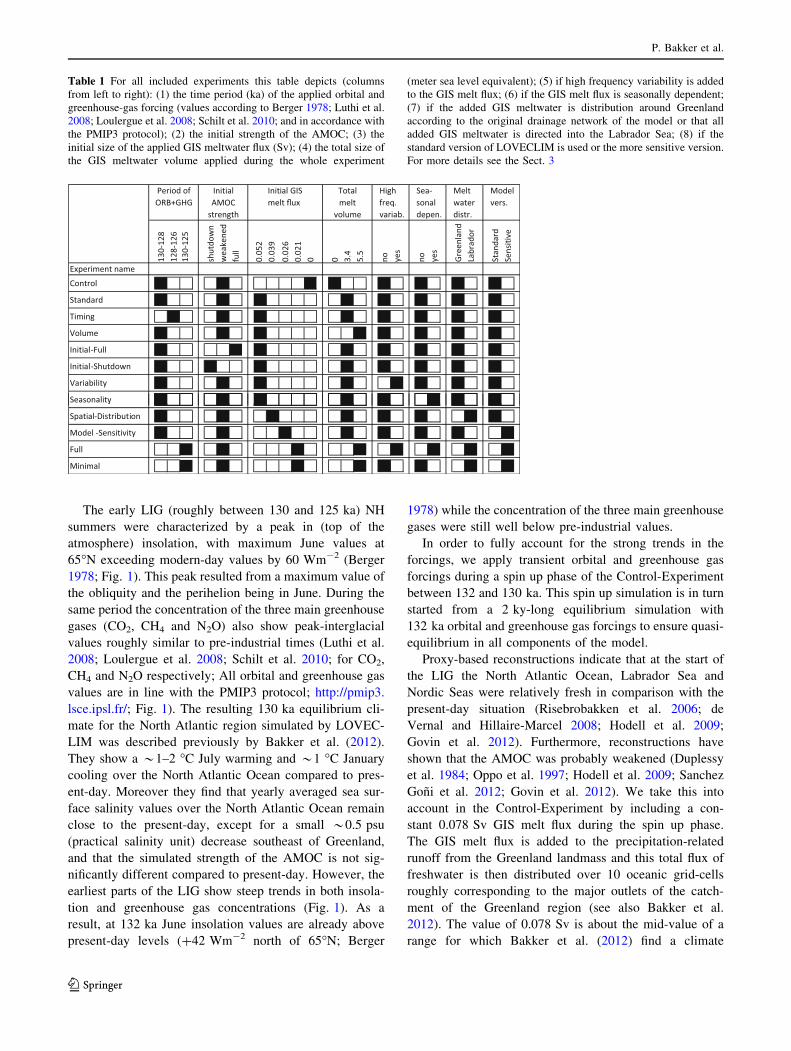
Table 1 For all included experiments this table depicts (columns

from left to right): (1) the time period (ka) of the applied orbital and

greenhouse-gas forcing (values according to Berger 1978; Luthi et al.

2008; Loulergue et al. 2008; Schilt et al. 2010; and in accordance with

the PMIP3 protocol); (2) the initial strength of the AMOC; (3) the

initial size of the applied GIS meltwater flux (Sv); (4) the total size of

the GIS meltwater volume applied during the whole experiment

(meter sea level equivalent); (5) if high frequency variability is added

to the GIS melt flux; (6) if the GIS melt flux is seasonally dependent;

(7) if the added GIS meltwater is distribution around Greenland

according to the original drainage network of the model or that all

added GIS meltwater is directed into the Labrador Sea; (8) if the

standard version of LOVECLIM is used or the more sensitive version.

For more details see the Sect. 3

P. Bakker et al.

123

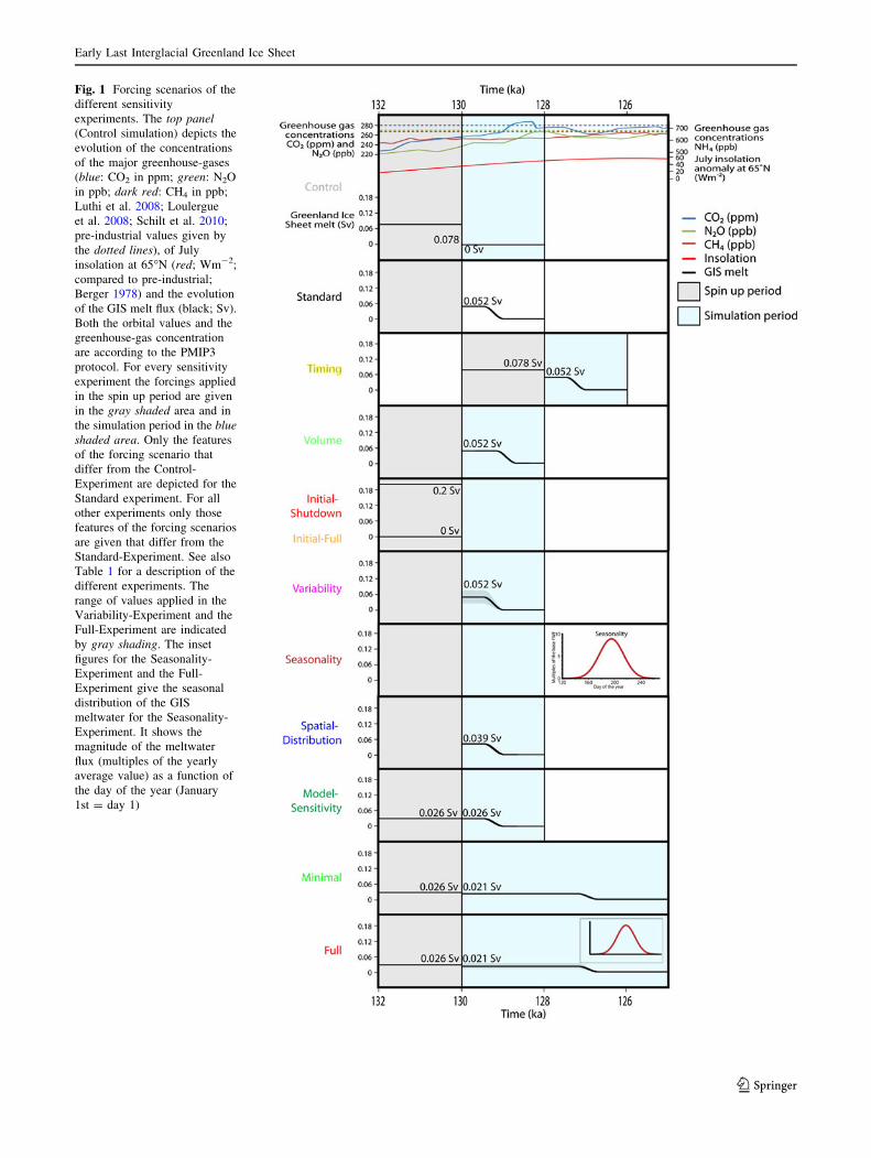
Fig. 1 Forcing scenarios of the

different sensitivity

experiments. The top panel

(Control simulation) depicts the

evolution of the concentrations

of the major greenhouse-gases

(blue: CO2 in ppm; green: N2O

in ppb; dark red: CH4 in ppb;

Luthi et al. 2008; Loulergue

et al. 2008; Schilt et al. 2010;

pre-industrial values given by

the dotted lines), of July

insolation at 65�N (red; Wm-2;

compared to pre-industrial;

Berger 1978) and the evolution

of the GIS melt flux (black; Sv).

Both the orbital values and the

greenhouse-gas concentration

are according to the PMIP3

protocol. For every sensitivity

experiment the forcings applied

in the spin up period are given

in the gray shaded area and in

the simulation period in the blue

shaded area. Only the features

of the forcing scenario that

differ from the Control-

Experiment are depicted for the

Standard experiment. For all

other experiments only those

features of the forcing scenarios

are given that differ from the

Standard-Experiment. See also

Table 1 for a description of the

different experiments. The

range of values applied in the

Variability-Experiment and the

Full-Experiment are indicated

by gray shading. The inset

figures for the Seasonality-

Experiment and the Full-

Experiment give the seasonal

distribution of the GIS

meltwater for the Seasonality-

Experiment. It shows the

magnitude of the meltwater

flux (multiples of the yearly

average value) as a function of

the day of the year (January

1st = day 1)

Early Last Interglacial Greenland Ice Sheet

123

regime with a weakened AMOC by about *30 % and no

deep convection in the Labrador Sea. The possible

implications of the choices made in this spin up procedure

will be investigated in the sensitivity experiment in Sect.

3.5. Apart from the spin up phase, no additional melt flux

is applied during the remaining 2 ky of the control

experiment (i.e. it is set to zero at 130 ka, or year 0 in

Fig. 2a). All experiments are limited to 2 ky unless the

impact of GIS melting on the AMOC persists after this

period. In all experiments in this manuscript, sea-level

height and ice sheets were fixed at their present-day

configuration. To summarize, the Control-Experiment is

thus forced solely by 130–128 ka orbital and greenhouse-

gas values, the AMOC is initially in a weakened state but

no GIS melt flux is added during the 130–128 ka simu-

lation period. In the following sensitivity experiments, the

imposed scenarios are identical to the Control-Experiment

described above unless specifically stated otherwise.

The evolution of the AMOC in the Control-Experiment

shows that the overturning recovers rapidly (i.e. within

*100 years) from the weakened state to full strength

(respectively around 13 and 24 Sv in this model; Fig. 2a).

Note that throughout this manuscript we will use the

maximum overturning streamfunction in the North Atlantic

to describe the strength of the AMOC.

3.2 Standard LIG GIS melt experiment

The described June insolation peak between 130 and

125 ka could have led to maximum GIS melt rates (Otto-

Bliesner et al. 2006) as ablation is particularly sensitive to

insolation during spring and early summer (Krabill et al.

2004; Otto-Bliesner et al. 2006). This suggested timing of

maximum GIS melt during the early LIG is corroborated

by findings in deep sea geochemical-proxies which indicate

a large and steady runoff between 132 and 120 ka (Carlson

et al. 2008) and a reconstructed minimal GIS configuration

around 127 ka (Lhomme et al. 2005). For this reason, in the

Standard-Experiment the GIS melt flux starts at 130 ka. In

the Standard-Experiment, a total of 3.4 msle (meter sea

level equivalent) is added to the ocean (after Otto-Bliesner

et al. 2006). This value is close to the estimates of Alley

et al. (2010) and Stone et al. (2013). In the Standard-

Experiment we first keep the melt rate constant at a value

of 0.052 Sv for 513 years. This GIS melt rate of 0.052 Sv

was taken from Bakker et al. (2012), who showed that, in

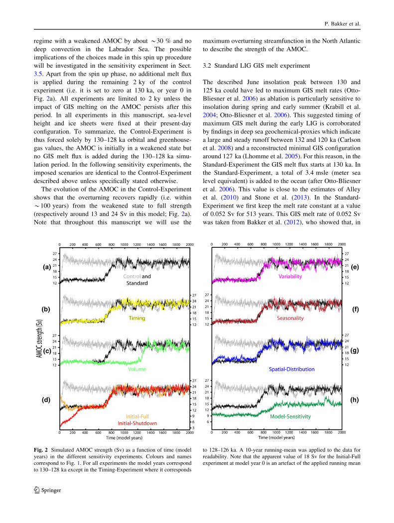
Fig. 2 Simulated AMOC strength (Sv) as a function of time (model

years) in the different sensitivity experiments. Colours and names

correspond to Fig. 1. For all experiments the model years correspond

to 130–128 ka except in the Timing-Experiment where it corresponds

to 128–126 ka. A 10-year running-mean was applied to the data for

readability. Note that the apparent value of 18 Sv for the Initial-Full

experiment at model year 0 is an artefact of the applied running mean

P. Bakker et al.

123

this experimental setup and model, this is the smallest

possible GIS melt flux for which a weakened AMOC state

without deep convection taking place in the Labrador Sea

can be maintained in our model. For a smaller melt flux the

AMOC switches back to the unperturbed situation. This

definition of the minimum GIS melt flux needed to main-

tain a weakened AMOC state will be used throughout the

manuscript in order to investigate any changes in the sen-

sitivity of the AMOC to GIS melt. The duration is set at

513 years in order to end up with a total volume of

3.4 msle. After 513 years with a constant rate, we decrease

the melt flux towards zero in 500 years following a sine

function (Fig. 1). Note that the 500 year length of this

decreasing part of the curve is arbitrary. Unfortunately, no

reconstructions are available that provide information on

the shape of the LIG GIS melt curve. However, we would

argue that a sinusoidal decrease is probably more realistic

than a linearly or abruptly decreasing melt flux, because the

melt flux is likely depending on the remaining volume of

the GIS. No intra-annual or inter-decadal variability is

added to the applied GIS melt rate in the Standard-

Experiment. The impact of these variabilities is however

investigated in Sects. 3.6 and 3.7. Similar to the GIS melt

flux of the spin up phase (Sect. 3.1), the described GIS melt

flux is distributed over the major outlets of the catchment

of the Greenland region. In the sensitivity experiment in

Sect. 3.8 we investigate the impact of this spatial distri-

bution of the GIS melt flux.

In the Standard-Experiment the imposed GIS melt keeps

the AMOC weakened for a period of 705 years. We define

the length of period of AMOC weakening as being the time

it takes before half the difference between the weakened

and full strength states of the AMOC has been overcome.

Afterwards the AMOC strength increases until the level of

the Control-Experiment is reached. Because in the Stan-

dard-Experiment the GIS melt flux decreases relatively

slowly after year 513, the transition period from a weak-

ened to a full strength AMOC state is somewhat longer,

*200 instead of *100 years, compared to the Control-

Experiment in which GIS melt is switched off abruptly at

the end of the spin up period (i.e. year 0 in Fig. 2a).

In the following sensitivity experiments, the imposed

scenarios are identical to the scenario of the Standard-

Experiment described above unless specifically stated

otherwise.

3.3 Timing of the period of enhanced GIS melt

Determining absolute ages for the LIG sea level curve is

difficult (Gallup et al. 2002; Kopp et al. 2009). It is

therefore hard to determine when all remnants of the NH

continental ice sheets had melted at the end of Termination

2 or when the period of enhanced GIS melting ended. This

could be important as Swingedouw et al. (2009b) showed

that the characteristics and the sensitivity of the AMOC can

differ significantly under different climatic settings. To test

the impact of the timing of the period of enhanced GIS

melt, we conducted a sensitivity experiment (hereafter

named Timing-Experiment) in which both the spin up

procedure and the actual forcing scenario were shifted

forward in time by 2 ky. This implies that the insolation

forcing and greenhouse gas concentrations in this Timing-

Experiment are different from the Standard-Experiment.

The 2 ky shift effectively means that the transient spin up

period of this Timing-Experiment now starts from a 130 ka

equilibrium simulation and includes transient orbital and

greenhouse-gas forcings between 130 and 128 ka while the

experiment itself is forced by 128–126 ka orbital and

greenhouse gas concentration changes (Fig. 1). The GIS

melt flux applied in the transient spin up period or during

the Timing-Experiment itself is identical to the Standard-

Experiment (Fig. 1).

The result of the Timing-Experiment shows that,

although there are small differences in the simulated evo-

lution of the AMOC compared to the Standard-Experiment,

these cannot be discerned from internal, unforced vari-

ability in the AMOC strength (Fig. 2b). We thus conclude

that, in this model a 2 ky uncertainty in the timing of the

period of enhanced LIG GIS melt does not have a clear

impact on the sensitivity of the AMOC to GIS melt. Note

that this experiment deals with changes in the insolation

forcing and greenhouse gas concentrations and does not

include any possible changes in the configuration of other

NH continental ice sheets which will be discussed in Sect. 5.

3.4 Volume of early LIG GIS melt

As mentioned previously there is considerable uncertainty

in the reconstructed volume loss of the GIS during the LIG.

In their review article, Alley et al. (2010) point out that

estimates are as low as 1 msle and up to the 5.5 msle

estimate of Cuffey and Marshall (2000; comparable to

volume losses of around 13 and 70 %, respectively). To

test the importance of the total volume of meltwater which

is introduced into the ocean we apply in this Volume-

Experiment a total of 5.5 msle rather than the 3.4 msle

used in the Standard-Experiment. This effectively means

that the 0.052 Sv GIS melt flux can be maintained for a

total of 980 years instead of the 513 years in the Standard-

Experiment (Fig. 1).

The resulting AMOC evolution in the Volume-Experi-

ment shows that the period of AMOC weakening under this

scenario is prolonged by 67 % from 705 to 1,174 years

(Fig. 2c).

Early Last Interglacial Greenland Ice Sheet

123

3.5 Initial state of the AMOC

During the deglaciation preceding the LIG period (Termi-

nation II), meltwater from the disintegrating NH conti-

nental ice sheets likely weakened the AMOC strength

(Duplessy et al. 1984; Oppo et al. 1997) and therewith

determined its characteristics at the start of the LIG. To test

the sensitivity of our results to the state of the AMOC at the

start of the transient GIS melt scenario we conducted two

experiments with different spin up procedures compared to

the Standard-Experiment. In the first one (Initial-Shut-

down-Experiment), we forced an AMOC shutdown during

the transient spin up phase by imposing a constant 0.2 Sv

melt flux (Fig. 1; value taken after Bakker et al. 2012). In

the second sensitivity experiment (Initial-Full-Experi-

ment), no melt flux was prescribed during the transient spin

up phase ensuring the simulation to start with an AMOC at

full strength.

In both the Initial-Shutdown-Experiment and the Initial-

Full-Experiment, the evolution of the AMOC strength

shows that it takes *200–400 years to get back to equi-

librium with the applied freshwater forcing (Fig. 2d). For

the remaining 1,800 years, the evolution of the AMOC

strength is very similar to the evolution in the Standard-

Experiment. It appears from the Initial-Shutdown-Experi-

ment and the Initial-Full-Experiment that, in LOVECLIM,

the choice of the initial state of the AMOC does not sig-

nificantly alter the impact of the partial melting of the GIS

on the evolution of the AMOC during the first thousand of

years of the early LIG. It must be noted that the total

volume of GIS meltwater released into the ocean during the

2 ky spin up phase differs between these experiments

(0 msle in the Initial-Full-Experiment, *9 msle in the

Standard-Experiment and *35 msle in the Initial-Shut-

down-Experiment). Furthermore, the duration of the period

over which the ocean is perturbed with a freshwater flux

could alter the final impact because of the long response

time of the deep ocean and the potential build up of a

thicker surface freshwater lid. Regardless of the large dif-

ferences in the initial state of the Initial-Shutdown-

Experiment and the Initial-Full-Experiment and the lack of

a clear impact on the succeeding AMOC evolution, we

cannot exclude that the total volume of freshwater or the

duration of the period over which the flux is applied

impacts the results.

3.6 Impact of high frequency variability

In the experiments described so far, the GIS melt flux has

been assumed constant on short timescales (sub-decadal).

This is justified as LIG GIS reconstructions have thus far

not resolved decadal-scale variability (Rohling et al. 2007;

Carlson et al. 2008). Notwithstanding, GIS melt

fluctuations with an amplitude of up to 50 % of the annual-

average have been observed over the last decades (Hanna

et al. 2008). It is therefore plausible that the freshwater flux

from the GIS during the early LIG exhibited similar short-

term variability. Loosely based on the observations of

Hanna et al. (2008), we therefore constructed a GIS melt

scenario for the Variability-Experiment in which fluctua-

tions, with an amplitude of 50 % of the standard forcing

and a periodicity of 6-years, are superimposed on the GIS

melt curve of the Standard-Experiment (Fig. 1). The

applied periodicity of 6-years is taken from the data of

Hanna et al. (2008) but we do note that they do not spe-

cifically describe any periodicity and it might well be that

the fluctuations are in reality more of a random nature.

The resulting evolution of the AMOC strength (Fig. 2e)

in the Variability-Experiment shows that, in comparison

with the Standard-Experiment, high frequency variability

in the GIS melt flux has no clear impact on either the long

term evolution or the decadal variability of the simulated

AMOC strength. If this conclusion would hold in higher

resolution models remains to be investigated.

3.7 Seasonal dependency of the GIS meltwater

In the experiments described so far we have assumed that

the GIS meltwater flux is constant throughout the year.

Although common practice in many previous so-called

water hosing experiments, this is obviously an oversim-

plification of the complex dependency of GIS runoff on

temperature and precipitation changes. This might prove

important since deep convection in the Labrador Sea area is

also strongly seasonally biased; both in observations and in

the LOVECLIM model, deep convection in the Labrador

Sea largely takes place between January and April. Here

we test the sensitivity of the AMOC to a seasonally

changing GIS runoff flux. In the setup of this Seasonality-

Experiment we make the GIS runoff flux a function of the

day of the year, loosely following the observations of

Wang et al. (2004). They describe how the melt extent of

the GIS changed throughout the year for the period

2000–2004. We made use of these findings by imposing a

melt season extending from early May to the end of Sep-

tember. In between, the magnitude of the melt extent fol-

lows a normal distribution with a peak runoff of almost 9

times the annual mean value (peak value at day 195 is 8.8

times the annual mean of 0.052 Sv yielding a peak flux of

0.46 Sv; the width of the curve corresponds to a standard

deviation of 44 days). In reality the situation is more

complex as the duration of the melt season differs per year

and per region (Wang et al. 2004). However, we consider

this simplified Seasonality-Experiment scenario sufficient

to investigate the sensitivity of the AMOC to seasonality of

the GIS melt flux.

P. Bakker et al.

123

The evolution of the AMOC strength in the Seasonality-

Experiment is very similar to the one simulated in the

Standard-Experiment (Fig. 2f). This sensitivity experiment

shows that in LOVECLIM, making the magnitude of the

GIS meltwater flux depend on the time of the year, does not

clearly impact the sensitivity of the AMOC to LIG GIS

melt.

3.8 Spatial distribution of GIS meltwater

Thus far, the additional GIS runoff has been distributed

evenly over the ocean waters bordering the 10 outlet points

defined in the model. This effectively means that a portion

of the GIS melt water flux enters the Arctic Ocean, Fram

Strait, the Labrador Sea and the Irminger Sea. LIG

reconstructions of the distributed of GIS meltwater over the

different rivers and outlet glaciers are not available. But

from observations it has been shown that nowadays a large

part of the runoff from Greenland, both by liquid water and

by the calving of iceberg, occurs around the southern tip as

well as along the west coast (van den Broeke et al. 2009).

In the Spatial-Distribution-Experiment we test, as an

extreme case, how the sensitivity of the AMOC to GIS

melting is affected if all GIS melt water is directed to the

outlet points closest to the Labrador Sea. This distribution

is chosen since introducing it directly into the Labrador Sea

likely yields the largest impact on Labrador Sea deep

convection and therewith on the AMOC strength. Although

we note that this is an extreme and probably unrealistic

scenario, it is useful to investigate the potential importance

of the spatial distribution of GIS meltwater.

The results of the Spatial-Distribution-Experiment show

that by concentrating the freshwater flux from the GIS into

the Labrador Sea, a stronger impact on the AMOC is

simulated. This was to be expected given that freshwater

entering the ocean outside of the Labrador Sea will be

diluted before reaching the deep convection site in the

Labrador Sea (c.f. Roche et al. 2010). Additional sensi-

tivity experiments have shown that in this scenario, 25 %

less freshwater is needed to maintain roughly the same

weakened AMOC state as in the Standard-Experiment

(0.039 Sv instead of 0.052 Sv; in Fig. 2 g only the former

simulation is shown). Consequently, this sensitivity

experiment reveals that in LOVECLIM, changing the

spatial distribution of the GIS meltwater flux alters the

sensitivity of the AMOC to LIG GIS melt.

3.9 Model dependency of the AMOCs sensitivity

to freshwater forcing

Even though the sensitivity of the AMOC to a perturbation

of the freshwater budget in LOVECLIM, is very similar to

other models (Rahmstorf et al. 2005; Stouffer et al. 2006;

Loutre et al. 2011), a comparison with ‘reality’ is difficult

as the actual sensitivity is largely unknown. All climate

models are tuned in various ways (Murphy et al. 2004) in

order to represent the characteristics of the present-day

climate. As shown by Loutre et al. (2011), there is more

than one set of parameters for LOVECLIM for which

simulated present-day temperatures and the evolution of

temperatures over the last century compares satisfactorily

with observations. Here we use the LOVECLIM parameter

set 322 that produces a relatively strong sensitivity of the

AMOC to freshwater forcing (i.e. in this version of the

model the AMOC decrease is roughly three times larger

after 1,000 years of linearly increasing freshwater forcing

up to 0.2 Sv compared to the standard version). This higher

AMOC sensitivity mainly results from a decrease of the

applied precipitation correction (Sect. 2) and small changes

in the albedo of sea ice and the vertical mixing of ocean

water. For a more detailed description of the changes

applied in this different parameter set the reader is referred

to Loutre et al. (2011). The AMOC sensitivity in this

alternative set up of the LOVECLIM model is at the

extreme high end of the range derived by Stouffer et al.

(2006); a 9.9 Sv decrease (50 % relative to the unperturbed

state; results not shown) of the AMOC strength compared

to an inter-model range of 1.3–9.7 Sv (9–62 %; Stouffer

et al. 2006; simulated change of AMOC strength after

perturbing the PI climate with a 0.1 Sv freshwater flux

applied to the North Atlantic Ocean between 50� and 70�N

over a period of 100 years).

For this Model-Sensitivity-Experiment a separate spin

up simulation was performed to ensure equilibrium of the

climate for this specific model-version. As for the Stan-

dard-Experiment, a 132 ka equilibrium climate was simu-

lated without additional GIS melting and a second transient

spin up simulation was performed including a constant GIS

melt rate. However the applied melt rate in the transient

spin up phase is only 0.026 Sv because additional experi-

ments showed that this flux has a comparable impact on the

AMOC in this more sensitive model version as a 0.078 Sv

meltwater flux has in the normal model version. The

meltwater scenario applied in this Model-Sensitivity-

Experiment during the 130–128 ka period is constant at

0.026 Sv for 513 years and thereafter follows a sinusoidal

curve towards a zero flux like in the other scenarios.

The resulting evolution of the AMOC in the Model-

Sensitivity-Experiment shows very similar behaviour as the

Standard-Experiment with a period of weakened AMOC, a

transition period and a period in which the AMOC returns

to the unperturbed full strength state (Fig. 2h). Note how-

ever that in this set up of the model, the absolute strength of

the AMOC in both the weakened and full states (9 and

15 Sv respectively) is lower than in the standard model

version (13 and 22 Sv respectively). Additional sensitivity

Early Last Interglacial Greenland Ice Sheet

123

experiments have shown that in this model set up and under

this scenario, 0.026 Sv instead of 0.052 Sv freshwater is

needed to maintain a weakened AMOC state compared to

the Standard-Experiment, about 50 % less (in Fig. 2h only

the results for a 0.026 Sv melt flux are shown). This

Model-Sensitivity-Experiment shows that the sensitivity of

the AMOC to LIG GIS melt can increase dramatically

when using a different parameter set in LOVECLIM.

4 Simulating the longest possible period of early LIG

AMOC weakening forced by GIS melting

within the parameter space of uncertainties

The performed sensitivity experiments give a clear insight

into the impact of the uncertainties related to GIS melting

on the strength of the AMOC during the early LIG in our

model. Small changes in the orbital and greenhouse gas

forcing, the initial state of the AMOC or the details of the

meltwater curve like high frequency variability or season-

ality do not significantly alter the sensitivity of the simu-

lated AMOC to early LIG GIS melt or prolong the period

of AMOC weakening. However, we also established three

factors that have a clear impact on the magnitude and

duration of the AMOC weakening: (1) the total volume of

GIS melt water added to the ocean, (2) the spatial distri-

bution of the GIS melt water and (3) the model-dependent

sensitivity of the AMOC.

Still, none of the individual sensitivity experiments

resulted in the 3–5 ky period of AMOC weakening as

suggested by proxy-data. In the next step we combine the

findings from the sensitivity experiments in the construc-

tion of two final early LIG GIS melt scenarios. We aim at

simulating the longest possible period of early LIG GIS

melt forced AMOC weakening while still being within the

parameter space of all described uncertainties. Firstly we

construct a Minimal-Experiment, including only those

forcings that have shown to enhance the AMOC sensitivity

to GIS melt or lengthen the period of AMOC weakening.

Therefore, we prescribe in the Minimal-Experiment a total

volume of GIS melt of 5.5 msle which all flows directly

into the Labrador Sea and we use the more sensitive ver-

sion of the model. Because of its simplicity, such a Mini-

mal-Experiment scenario could potentially be used for

simulations with other climate models in order to evaluate

the AMOC sensitivity to GIS melt. Secondly we construct

a Full-Experiment that, on top of the forcings described for

the Minimal-Experiment, includes also high-frequency

variability and a seasonal dependence of the GIS melt flux,

in closer resemblance of present-day observations of GIS

melt.

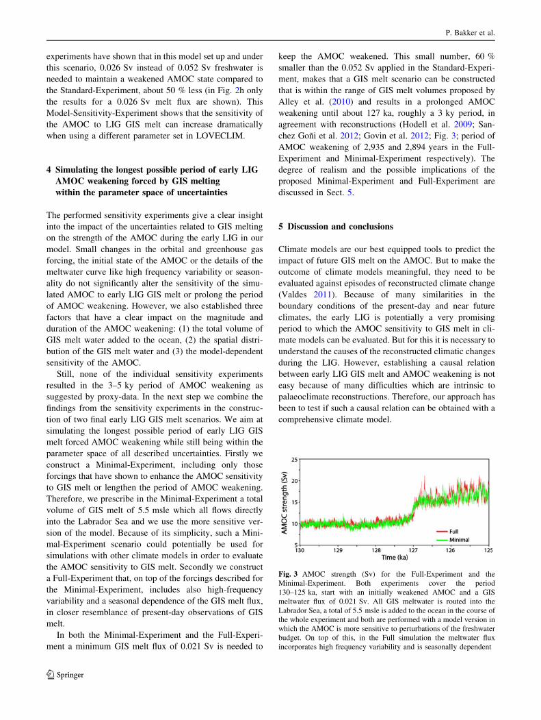
In both the Minimal-Experiment and the Full-Experi-

ment a minimum GIS melt flux of 0.021 Sv is needed to

keep the AMOC weakened. This small number, 60 %

smaller than the 0.052 Sv applied in the Standard-Experi-

ment, makes that a GIS melt scenario can be constructed

that is within the range of GIS melt volumes proposed by

Alley et al. (2010) and results in a prolonged AMOC

weakening until about 127 ka, roughly a 3 ky period, in

agreement with reconstructions (Hodell et al. 2009; San-

chez Goni et al. 2012; Govin et al. 2012; Fig. 3; period of

AMOC weakening of 2,935 and 2,894 years in the Full-

Experiment and Minimal-Experiment respectively). The

degree of realism and the possible implications of the

proposed Minimal-Experiment and Full-Experiment are

discussed in Sect. 5.

5 Discussion and conclusions

Climate models are our best equipped tools to predict the

impact of future GIS melt on the AMOC. But to make the

outcome of climate models meaningful, they need to be

evaluated against episodes of reconstructed climate change

(Valdes 2011). Because of many similarities in the

boundary conditions of the present-day and near future

climates, the early LIG is potentially a very promising

period to which the AMOC sensitivity to GIS melt in cli-

mate models can be evaluated. But for this it is necessary to

understand the causes of the reconstructed climatic changes

during the LIG. However, establishing a causal relation

between early LIG GIS melt and AMOC weakening is not

easy because of many difficulties which are intrinsic to

palaeoclimate reconstructions. Therefore, our approach has

been to test if such a causal relation can be obtained with a

comprehensive climate model.

Fig. 3 AMOC strength (Sv) for the Full-Experiment and the

Minimal-Experiment. Both experiments cover the period

130–125 ka, start with an initially weakened AMOC and a GIS

meltwater flux of 0.021 Sv. All GIS meltwater is routed into the

Labrador Sea, a total of 5.5 msle is added to the ocean in the course of

the whole experiment and both are performed with a model version in

which the AMOC is more sensitive to perturbations of the freshwater

budget. On top of this, in the Full simulation the meltwater flux

incorporates high frequency variability and is seasonally dependent

P. Bakker et al.

123

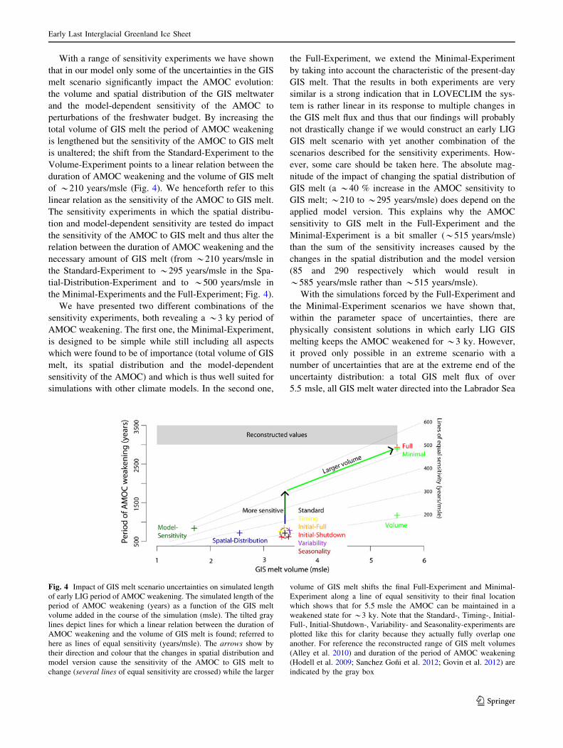
With a range of sensitivity experiments we have shown

that in our model only some of the uncertainties in the GIS

melt scenario significantly impact the AMOC evolution:

the volume and spatial distribution of the GIS meltwater

and the model-dependent sensitivity of the AMOC to

perturbations of the freshwater budget. By increasing the

total volume of GIS melt the period of AMOC weakening

is lengthened but the sensitivity of the AMOC to GIS melt

is unaltered; the shift from the Standard-Experiment to the

Volume-Experiment points to a linear relation between the

duration of AMOC weakening and the volume of GIS melt

of *210 years/msle (Fig. 4). We henceforth refer to this

linear relation as the sensitivity of the AMOC to GIS melt.

The sensitivity experiments in which the spatial distribu-

tion and model-dependent sensitivity are tested do impact

the sensitivity of the AMOC to GIS melt and thus alter the

relation between the duration of AMOC weakening and the

necessary amount of GIS melt (from *210 years/msle in

the Standard-Experiment to *295 years/msle in the Spa-

tial-Distribution-Experiment and to *500 years/msle in

the Minimal-Experiments and the Full-Experiment; Fig. 4).

We have presented two different combinations of the

sensitivity experiments, both revealing a *3 ky period of

AMOC weakening. The first one, the Minimal-Experiment,

is designed to be simple while still including all aspects

which were found to be of importance (total volume of GIS

melt, its spatial distribution and the model-dependent

sensitivity of the AMOC) and which is thus well suited for

simulations with other climate models. In the second one,

the Full-Experiment, we extend the Minimal-Experiment

by taking into account the characteristic of the present-day

GIS melt. That the results in both experiments are very

similar is a strong indication that in LOVECLIM the sys-

tem is rather linear in its response to multiple changes in

the GIS melt flux and thus that our findings will probably

not drastically change if we would construct an early LIG

GIS melt scenario with yet another combination of the

scenarios described for the sensitivity experiments. How-

ever, some care should be taken here. The absolute mag-

nitude of the impact of changing the spatial distribution of

GIS melt (a *40 % increase in the AMOC sensitivity to

GIS melt; *210 to *295 years/msle) does depend on the

applied model version. This explains why the AMOC

sensitivity to GIS melt in the Full-Experiment and the

Minimal-Experiment is a bit smaller (*515 years/msle)

than the sum of the sensitivity increases caused by the

changes in the spatial distribution and the model version

(85 and 290 respectively which would result in

*585 years/msle rather than *515 years/msle).

With the simulations forced by the Full-Experiment and

the Minimal-Experiment scenarios we have shown that,

within the parameter space of uncertainties, there are

physically consistent solutions in which early LIG GIS

melting keeps the AMOC weakened for *3 ky. However,

it proved only possible in an extreme scenario with a

number of uncertainties that are at the extreme end of the

uncertainty distribution: a total GIS melt flux of over

5.5 msle, all GIS melt water directed into the Labrador Sea

Fig. 4 Impact of GIS melt scenario uncertainties on simulated length

of early LIG period of AMOC weakening. The simulated length of the

period of AMOC weakening (years) as a function of the GIS melt

volume added in the course of the simulation (msle). The tilted gray

lines depict lines for which a linear relation between the duration of

AMOC weakening and the volume of GIS melt is found; referred to

here as lines of equal sensitivity (years/msle). The arrows show by

their direction and colour that the changes in spatial distribution and

model version cause the sensitivity of the AMOC to GIS melt to

change (several lines of equal sensitivity are crossed) while the larger

volume of GIS melt shifts the final Full-Experiment and Minimal-

Experiment along a line of equal sensitivity to their final location

which shows that for 5.5 msle the AMOC can be maintained in a

weakened state for *3 ky. Note that the Standard-, Timing-, Initial-

Full-, Initial-Shutdown-, Variability- and Seasonality-experiments are

plotted like this for clarity because they actually fully overlap one

another. For reference the reconstructed range of GIS melt volumes

(Alley et al. 2010) and duration of the period of AMOC weakening

(Hodell et al. 2009; Sanchez Goni et al. 2012; Govin et al. 2012) are

indicated by the gray box

Early Last Interglacial Greenland Ice Sheet

123

and a climate model with a relatively high sensitivity to an

anomalous freshwater forcing compared to other climate

models. This makes that the likelihood of the Full-Exper-

iment and the Minimal-Experiment, given by the product

of individual likelihoods, is extremely low. Assuming that

our models have a reasonable sensitivity to freshwater

forcing, this is a strong indication that early LIG GIS melt

alone did not result in the AMOC weakening. However,

there are two remaining possibilities that we will discuss

hereafter: forcings missing from the simulations explain

the AMOC weakening or early LIG GIS melt forced the

AMOC into another branch of a bi-stable regime which is

not present in our simulations.

There are several other forcings that might have played

a role in keeping the strength of the AMOC reduced during

the early part of the LIG. Firstly, the meltwater fluxes

during the deglaciation preceding the LIG (i.e. Termination

II) are different from the last deglaciation. For instance the

Eurasian Ice Sheet was relatively large during the penul-

timate glacial compared to the last glacial (e.g. Svendsen

et al. 2004). This might have introduced a larger meltwater

flux into the Nordic Seas, including the deep convection

areas that have been shown to be especially sensitive to

meltwater (Roche et al. 2010). Also the deglacial history of

the Antarctic Ice Sheet (AIS) was inferred to be rather

different during Termination I than during Termination II,

with an estimated 40 % larger mass loss during the latter

(5.8 m compared to 4.1 msle; McKay et al. 2011). An

enhanced melt flux of the AIS has been shown to poten-

tially weaken the AMOC although the impact is highly

dependent on the size of the imposed melt flux (Swinge-

douw et al. 2009a).

Another possible mechanism that could explain the

weak AMOC in the early LIG involves a different stability

regime. The AMOC is thought to involve a number of non-

linear feedbacks that can lead to so-called hysteresis

behaviour. This implies that multiple equilibrium states can

exist and that the AMOC can be mono-stable or bi-stable,

the latter indicating that an AMOC collapse is irreversible

even if the fresh water perturbation ceases (Stommel 1961;

Rahmstorf et al. 2005). Most likely the AMOC in all

coupled atmosphere–ocean models exhibits hysteresis

behaviour (Rahmstorf et al. 2005), but the shape of the

hysteresis curve as well as the position of the present-day

climate on this curve are strongly dependent on the back-

ground climate and on the set up and tuning of the model

under consideration (Hofmann and Rahmstorf 2009). The

AMOCs hysteresis behaviour in the LOVECLIM model

has previously been shown to be in the range of atmo-

sphere–ocean general circulation models (Rahmstorf et al.

2005; Stouffer et al. 2006) and shown to be mono-stable

under present-day (PI) boundary conditions while it is bi-

stable in a Last Glacial Maximum climate (Kageyama et al.

2010). During the LIG the stability of the AMOC might

also have been significantly different from present-day, for

instance because of changes in the seasonal cycle of sea ice

as described by Born et al. (2010). So what are the char-

acteristics of the AMOCs behaviour simulated by

LOVECLIM under LIG boundary conditions? And how

does this change when the more sensitive version of the

model is used? A first indication towards a mono-stable

AMOC is found in the experiments presented so far

because in none of them did the AMOC remain weakened

long after the freshwater perturbation had ceased.

To further investigate the AMOC hysteresis behaviour,

three additional experiments have been performed to assess

the difference between the LIG and PI and to assess the

impact of a different tuning of the model. To compute the

hysteresis curves we follow Kageyama et al. (2010) by

applying a freshwater forcing to the surface of the Atlantic

Ocean between 50� and 70�N. This forcing linearly

increases in 6 ky from 0 to 0.3 Sv, then linearly decreases

in 7 ky from 0.3 to -0.05 Sv and then linearly returns to

0 Sv in another 1 ky. This freshwater forcing scenario was

applied to an equilibrium simulation of the present-day

climate with the normal model version (PI_E00) and to a

LIG (128 ka) equilibrium simulation with both the normal

and the more sensitive model version of LOVECLIM

(LIG_E00 and LIG_E22 respectively). Note that in these

hysteresis experiments the freshwater forcing is applied

between 50� and 70�N while in all experiments described

above it was applied around Greenland. This was done to

be more in line with previous studies into the hysteresis

behaviour of the AMOC. Furthermore, it is not expected to

influence the actual hysteresis behaviour or the simulated

position of the present-day AMOC but only to shift the

hysteresis curve to the left or right. The results show that

the AMOC simulated by LOVECLIM is mono-stable for

both PI, the LIG and in both model versions (Fig. 5). The

simulated hysteresis curves PI_E00 and LIG_E00 reveal

very similar AMOC behaviour. Only for freshwater per-

turbation values over *0.15 Sv, it appears that the LIGs

AMOC has a slightly higher sensitivity. Furthermore, the

size and position of the vertical steps in the hysteresis

curves, indicative of shifts in the location of the main

convection site (Rahmstorf 1995), differ between the

PI_E00 and the LIG_E00 simulations. The steepness of the

hysteresis curve for LIG_E22 shows a higher sensitivity of

the AMOC to perturbations of the freshwater budget in this

model version compared to the standard model version. In

addition, the hysteresis behaviour in the LIG_E22 simu-

lation is shifted towards the unperturbed state by *0.1 Sv

relative to LIG_E00, indicating that a smaller change in the

climate is needed to shift the system into a bi-stable

regime. Only part of this shift can be explained by the

decrease in the applied precipitation correction

P. Bakker et al.

123

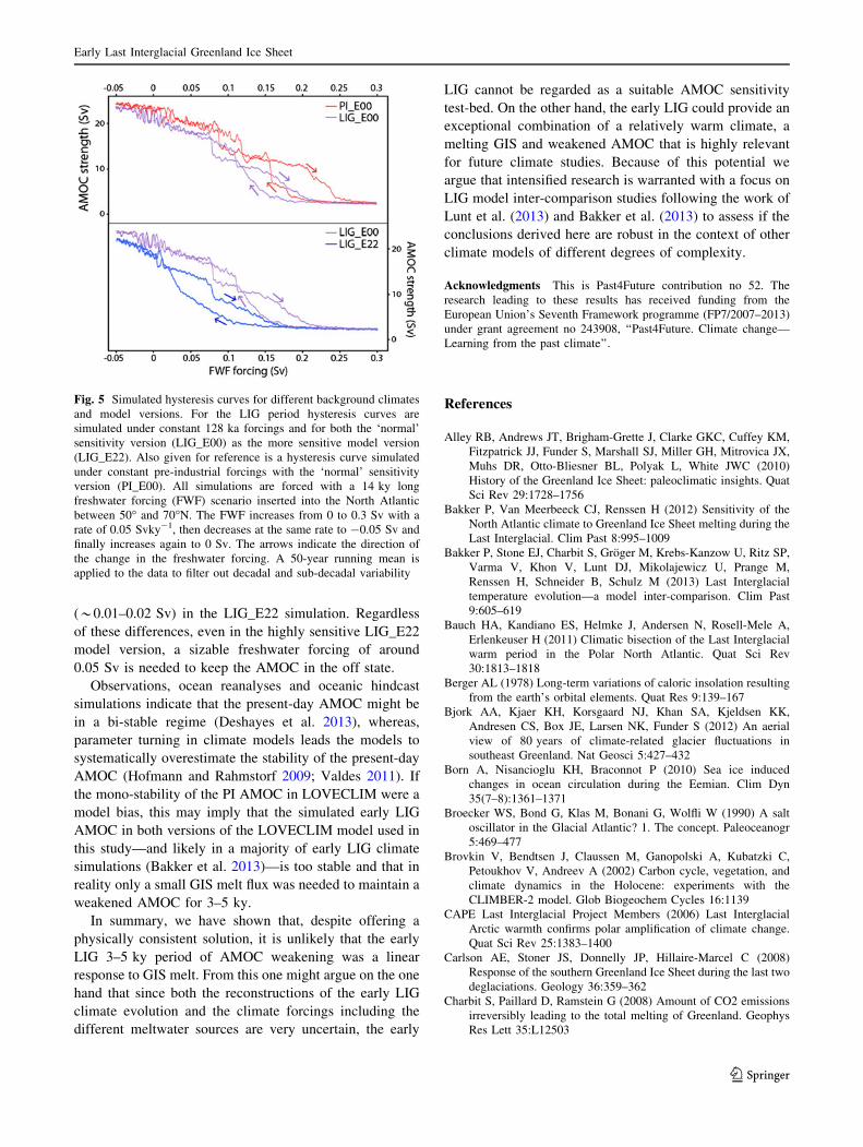
(*0.01–0.02 Sv) in the LIG_E22 simulation. Regardless

of these differences, even in the highly sensitive LIG_E22

model version, a sizable freshwater forcing of around

0.05 Sv is needed to keep the AMOC in the off state.

Observations, ocean reanalyses and oceanic hindcast

simulations indicate that the present-day AMOC might be

in a bi-stable regime (Deshayes et al. 2013), whereas,

parameter turning in climate models leads the models to

systematically overestimate the stability of the present-day

AMOC (Hofmann and Rahmstorf 2009; Valdes 2011). If

the mono-stability of the PI AMOC in LOVECLIM were a

model bias, this may imply that the simulated early LIG

AMOC in both versions of the LOVECLIM model used in

this study—and likely in a majority of early LIG climate

simulations (Bakker et al. 2013)—is too stable and that in

reality only a small GIS melt flux was needed to maintain a

weakened AMOC for 3–5 ky.

In summary, we have shown that, despite offering a

physically consistent solution, it is unlikely that the early

LIG 3–5 ky period of AMOC weakening was a linear

response to GIS melt. From this one might argue on the one

hand that since both the reconstructions of the early LIG

climate evolution and the climate forcings including the

different meltwater sources are very uncertain, the early

LIG cannot be regarded as a suitable AMOC sensitivity

test-bed. On the other hand, the early LIG could provide an

exceptional combination of a relatively warm climate, a

melting GIS and weakened AMOC that is highly relevant

for future climate studies. Because of this potential we

argue that intensified research is warranted with a focus on

LIG model inter-comparison studies following the work of

Lunt et al. (2013) and Bakker et al. (2013) to assess if the

conclusions derived here are robust in the context of other

climate models of different degrees of complexity.

Acknowledgments This is Past4Future contribution no 52. The

research leading to these results has received funding from the

European Union’s Seventh Framework programme (FP7/2007–2013)

under grant agreement no 243908, ‘‘Past4Future. Climate change—

Learning from the past climate’’.

References

Alley RB, Andrews JT, Brigham-Grette J, Clarke GKC, Cuffey KM,

Fitzpatrick JJ, Funder S, Marshall SJ, Miller GH, Mitrovica JX,

Muhs DR, Otto-Bliesner BL, Polyak L, White JWC (2010)

History of the Greenland Ice Sheet: paleoclimatic insights. Quat

Sci Rev 29:1728–1756

Bakker P, Van Meerbeeck CJ, Renssen H (2012) Sensitivity of the

North Atlantic climate to Greenland Ice Sheet melting during the

Last Interglacial. Clim Past 8:995–1009

Bakker P, Stone EJ, Charbit S, Groger M, Krebs-Kanzow U, Ritz SP,

Varma V, Khon V, Lunt DJ, Mikolajewicz U, Prange M,

Renssen H, Schneider B, Schulz M (2013) Last Interglacial

temperature evolution—a model inter-comparison. Clim Past

9:605–619

Bauch HA, Kandiano ES, Helmke J, Andersen N, Rosell-Mele A,

Erlenkeuser H (2011) Climatic bisection of the Last Interglacial

warm period in the Polar North Atlantic. Quat Sci Rev

30:1813–1818

Berger AL (1978) Long-term variations of caloric insolation resulting

from the earth’s orbital elements. Quat Res 9:139–167

Bjork AA, Kjaer KH, Korsgaard NJ, Khan SA, Kjeldsen KK,

Andresen CS, Box JE, Larsen NK, Funder S (2012) An aerial

view of 80 years of climate-related glacier fluctuations in

southeast Greenland. Nat Geosci 5:427–432

Born A, Nisancioglu KH, Braconnot P (2010) Sea ice induced

changes in ocean circulation during the Eemian. Clim Dyn

35(7–8):1361–1371

Broecker WS, Bond G, Klas M, Bonani G, Wolfli W (1990) A salt

oscillator in the Glacial Atlantic? 1. The concept. Paleoceanogr

5:469–477

Brovkin V, Bendtsen J, Claussen M, Ganopolski A, Kubatzki C,

Petoukhov V, Andreev A (2002) Carbon cycle, vegetation, and

climate dynamics in the Holocene: experiments with the

CLIMBER-2 model. Glob Biogeochem Cycles 16:1139

CAPE Last Interglacial Project Members (2006) Last Interglacial

Arctic warmth confirms polar amplification of climate change.

Quat Sci Rev 25:1383–1400

Carlson AE, Stoner JS, Donnelly JP, Hillaire-Marcel C (2008)

Response of the southern Greenland Ice Sheet during the last two

deglaciations. Geology 36:359–362

Charbit S, Paillard D, Ramstein G (2008) Amount of CO2 emissions

irreversibly leading to the total melting of Greenland. Geophys

Res Lett 35:L12503

Fig. 5 Simulated hysteresis curves for different background climates

and model versions. For the LIG period hysteresis curves are

simulated under constant 128 ka forcings and for both the ‘normal’

sensitivity version (LIG_E00) as the more sensitive model version

(LIG_E22). Also given for reference is a hysteresis curve simulated

under constant pre-industrial forcings with the ‘normal’ sensitivity

version (PI_E00). All simulations are forced with a 14 ky long

freshwater forcing (FWF) scenario inserted into the North Atlantic

between 50� and 70�N. The FWF increases from 0 to 0.3 Sv with a

rate of 0.05 Svky-1, then decreases at the same rate to -0.05 Sv and

finally increases again to 0 Sv. The arrows indicate the direction of

the change in the freshwater forcing. A 50-year running mean is

applied to the data to filter out decadal and sub-decadal variability

Early Last Interglacial Greenland Ice Sheet

123

Colville EJ, Carlson AE, Beard BL, Hatfield RG, Stoner JS, Reyes

AV, Ullman DJ (2011) Sr-Nd-Pb isotope evidence for Ice-Sheet

Presence on Southern Greenland during the Last Interglacial.

Science 333:620–623

Cuffey KM, Marshall SJ (2000) Substantial contribution to sea-level

rise during the Last Interglacial from the Greenland Ice Sheet.

Nature 404:591–594

de Vernal A, Hillaire-Marcel C (2008) Natural variability of

Greenland climate, vegetation, and ice volume during the past

million years. Science 320:1622–1625

Deshayes J, Treguier AM, Barnier B, Lecointre A, Le Sommer J,

Molines JM, Penduff T, Bourdalle-Badie R, Drillet Y, Garric G,

Benshila R, Madec G, Biastoch A, Boning CW, Scheinert M,

Coward AC, Hirschi JJM (2013) Oceanic hindcast simulations at

high resolution suggest that the Atlantic MOC is bistable.

Geophys Res Lett 40:3069–3073

Driesschaert E, Fichefet T, Goosse H, Huybrechts P, Janssens I,

Mouchet A, Munhoven G, Brovkin V, Weber SL (2007)

Modeling the influence of Greenland Ice Sheet melting on the

Atlantic meridional overturning circulation during the next

millennia. Geophys Res Lett 34:L10707

Duplessy JC, Shackleton NJ, Matthews RK, Prell W, Ruddiman WF,

Caralp M, Hendy CH (1984) 13C Record of benthic foraminifera

in the Last Interglacial ocean: implications for the carbon cycle

and the global deep water circulation. Quat Res 21:225–243

Gallup CD, Cheng H, Taylor FW, Edwards RL (2002) Direct

determination of the timing of sea level change during termi-

nation II. Science 295:310–313

Goosse H, Fichefet T (1999) Importance of ice-ocean interactions for

the global ocean circulation: a model study. J Geophys Res

104:23337–23355

Goosse H, Brovkin V, Fichefet T, Haarsma RJ, Huybrechts P, Jongma

JI, Mouchet A, Selten FM, Barriat P, Campin J, Renssen H,

Roche DM, Timmermann A, Opsteegh JD (2010) Description of

the Earth system model of intermediate complexity LOVECLIM

version 1.2. Geosci Mod Dev 3:309–390

Govin A, Braconnot P, Capron E, Cortijo E, Duplessy JC, Jansen E,

Labeyrie L, Landais A, Marti O, Michel E, Mosquet E,

Risebrobakken B, Swingedouw D, Waelbroeck C (2012) Persis-

tent influence of ice sheet melting on high northern latitude

climate during the early Last Interglacial. Clim Past 8:483–507

Hanna E, Huybrechts P, Steffen K, Cappelen J, Huff R, Shuman C,

Irvine-Fynn T, Wise S, Griffiths M (2008) Increased runoff from

melt from the Greenland Ice Sheet: a response to global

warming. J Clim 21:331–341

Hillaire-Marcel C, de Vernal A, Bilodeau G, Weaver AJ (2001)

Absence of deep-water formation in the Labrador Sea during the

Last Interglacial period. Nature 410:1073–1077

Hodell DA, Minth EK, Curtis JH, McCave IN, Hall IR, Channell JET,

Xuan C (2009) Surface and deep-water hydrography on Gardar

Drift (Iceland Basin) during the Last Interglacial period. Earth

Plan Sci Lett 288:10–19

Hofmann M, Rahmstorf S (2009) On the stability of the Atlantic

meridional overturning circulation. PNAS 106:20584–20589

Huybrechts P, de Wolde J (1999) The dynamic response of the

Greenland and Antarctic Ice Sheets to multiple-century climatic

warming. J Clim 12:2169–2188

Huybrechts P, Letreguilly A, Reeh N (1991) The Greenland Ice Sheet

and greenhouse warming. P3 89:399–412

Jungclaus JH, Haak H, Esch M, Roeckner E, Marotzke JW (2006)

Will Greenland melting halt the thermohaline circulation?

Geophys Res Lett 33:L17708

Kageyama M, Paul A, Roche DM, Van Meerbeeck CJ (2010)

Modelling glacial climatic millennial-scale variability related to

changes in the Atlantic meridional overturning circulation: a

review. Quat Sci Rev 29:2931–2956

Koerner RM (1989) Ice core evidence for extensive melting of the

Greenland Ice Sheet in the Last Interglacial. Science

244:964–968

Kopp RE, Simons FJ, Mitrovica JX, Maloof AC, Oppenheimer M

(2009) Probabilistic assessment of sea level during the Last

Interglacial stage. Nature 462:863–867

Krabill W, Hanna E, Huybrechts P, Abdalati W, Cappelen J, Csatho

B, Frederick E, Manizade S, Martin C, Sonntag J, Swift R,

Thomas R, Yungel J (2004) Greenland Ice Sheet: increased

coastal thinning. Geophys Res Lett 31:L24402

Kukla GJ, Bender ML, de Beaulieu JL, Bond G, Broecker WS,

Cleveringa P, Gavin JE, Herbert TD, Imbrie J, Jouzel J, Keigwin

LD, Knudsen KL, McManus JF, Merkt J, Muhs DR, Muller H,

Poore RZ, Porter SC, Seret G, Shackleton NJ, Turner C,

Tzedakis PC, Winograd IJ (2002) Last Interglacial climates.

Quat Res 58:2–13

Lhomme N, Clarke GKC, Marshall SJ (2005) Tracer transport in the

Greenland Ice Sheet: constraints on ice cores and glacial history.

Quat Sci Rev 24:173–194

Loulergue L, Schilt A, Spahni R, Masson-Delmotte V, Blunier T,

Lemieux B, Barnola JM, Raynaud D, Stocker TF, Chappellaz J

(2008) Orbital and millennial-scale features of atmospheric CH4

over the past 800,000 years. Nature 453:383–386

Loutre MF, Mouchet A, Fichefet T, Goosse H, Goelzer H, Huybrechts

P (2011) Evaluating climate model performance with various

parameter sets using observations over the recent past. Clim Past

7:511–526

Lunt DJ, Abe-Ouchi A, Bakker P, Berger A, Braconnot P, Charbit S,

Fischer N, Herold N, Jungclaus JH, Khon VC, Krebs-Kanzow U,

Langebroek PM, Lohmann G, Nisancioglu KH, Otto-Bliesner

BL, Park W, Pfeiffer M, Phipps SJ, Prange M, Rachmayani R,

Renssen H, Rosenbloom N, Schneider B, Stone EJ, Takahashi K,

Wei W, Yin Q, Zhang ZS (2013) A multi-model assessment of

Last Interglacial temperatures. Clim Past 9:699–717

Luthi D, Le Floch M, Bereiter B, Blunier T, Barnola JM, Siegenthaler

U, Raynaud D, Jouzel J, Fischer H, Kawamura K, Stocker TF

(2008) High-resolution carbon dioxide concentration record

650,000-800,000 years before present. Nature 453:379–382

Marshall J, Schott F (1999) Open-ocean convection: observations,

theory and models. Rev Geophys 37:1–64

McKay NP, Overpeck JT, Otto-Bliesner BL (2011) The role of ocean

thermal expansion in Last Interglacial sea level rise. Geophys

Res Lett 38:L14605

Murphy JM, Sexton DMH, Barnett DN, Jones GS, Webb MJ, Collins

M, Stainforth DA (2004) Quantification of modelling uncertain-

ties in a large ensemble of climate change simulations. Nature

430:768–772

NEEM community members (2013) Eemian interglacial recon-

structed from a Greenland folded ice core. Nature 493:489–494Oppo DW, Horowitz M, Lehman SJ (1997) Marine Core Evidence for

Reduced Deep Water Production during Termination II Fol-

lowed by a Relatively Stable Substage 5e (Eemian). Paleocea-

nography 12:51–63

Opsteegh JD, Haarsma RJ, Selten FM, Kattenberg A (1998) ECBILT:

a dynamic alternative to mixed boundary conditions in ocean

models. Tellus A 50:348–367

Otto-Bliesner BL, Marshall SJ, Overpeck JT, Miller GH, Hu A (2006)

Simulating arctic climate warmth and icefield retreat in the last

interglaciation. Science 311:1751–1753

Rahmstorf S (1995) Bifurcations of the Atlantic thermohaline

circulation in response to changes in the hydrological cycle.

Nature 378:145–149

Rahmstorf S, Crucifix M, Ganopolski A, Goosse H, Kamenkovich I,

Knutti R, Lohmann G, Marsh R, Mysak LA, Wang Z, Weaver

AJ (2005) Thermohaline circulation hysteresis: a model inter-

comparison. Geophys Res Lett 32:L23605

P. Bakker et al.

123

Rasmussen TL, Thomsen E, Kuijpers A, Wastegard S (2003) Late

warming and early cooling of the sea surface in the Nordic seas

during MIS 5e (Eemian Interglacial). Quat Sci Rev 22:809–821

Rayner D, Hirschi JJM, Kanzow T, Johns WE, Wright PG, Frajka-

Williams E, Bryden HL, Meinen CS, Baringer MO, Marotzke J,

Beal LM, Cunningham SA (2011) Monitoring the Atlantic

meridional overturning circulation. Deep Sea Res Part II Top

Stud Oceanogr 58:17–18

Renssen H, Seppa H, Heiri O, Roche DM, Goosse H, Fichefet T

(2009) The spatial and temporal complexity of the Holocene

thermal maximum. Nat Geosci 2:411–414

Ridley JK, Huybrechts P, Gregory JM, Lowe JA (2005) Elimination

of the Greenland Ice Sheet in a high CO2 climate. J Clim

18:3409–3427

Rignot E, Velicogna I, van den Broeke MR, Monaghan A, Lenaerts J

(2011) Acceleration of the contribution of the Greenland and

Antarctic ice sheets to sea level rise. Geophys Res Lett

38:L05503

Risebrobakken B, Balbon E, Dokken T, Jansen E, Kissel C, Labeyrie

L, Richter T, Senneset L (2006) The penultimate deglaciation:

high-resolution paleoceanographic evidence from a north-south

transect along the eastern Nordic Seas. Earth Plan Sci Lett

241:505–516

Roche DM, Wiersma AP, Renssen H (2010) A systematic study of the

impact of freshwater pulses with respect to different geographic

locations. Clim Dyn 34:997–1013

Rohling EJ, Grant K, Hemleben Ch, Siddal M, Hoogakker BAA,

Bolshaw M, Kucera M (2007) High rates of sea-level rise during

the Last Interglacial period. Nat Geosci 1:38–42

Sanchez Goni MF, Bakker P, Desprat S, Carlson AE, Van Meerbeeck

CJ, Peyron O, Naughton F, Fletcher WJ, Eynaud F, Rossignol L,

Renssen H (2012) European climate optimum and enhanced

Greenland melt during the Last Interglacial. Geology

40:627–630

Schilt A, Baumgartner M, Blunier T, Schwander J, Spahni R, Fischer

H, Stocker TF (2010) Glacial-interglacial and millennial-scale

variations in the atmospheric nitrous oxide concentration during

the last 800,000 years. Quat Sci Rev 29:182–192

Solomon SD, Qin D, Manning M, Chen Z, Marquis M, Averyt KB,

Tgnor M, Miller HL, IPCC (2007) Climate change 2007: the

physical science basis. Contribution of Working Group I to the

Fourth Assessment Report of the Intergovernmental Panel on

Climate Change. Cambridge University Press, Cambridge, p 996

Stommel H (1961) Thermohaline convection with two stable regimes

of flow. Tellus 13:224–230

Stone EJ, Lunt DJ, Annan JD, Hargreaves JC (2013) Quantification of

the Greenland Ice Sheet contribution to Last Interglacial sea

level rise. Clim Past 9:621–639

Stouffer RJ, Yin J, Gregory JM, Dixon KW, Spelman MJ, Hurlin W,

Weaver AJ, Eby M, Flato GM, Hasumi H, Hu A, Jungclaus JH,

Kamenkovich IV, Levermann A, Montoya M, Murakami S,

Nawrath S, Oka A, Peltier WR, Robitaille DY, Sokolov A,

Vettoretti G, Weber SL (2006) Investigating the causes of the

response of the thermohaline circulation to past and future

climate changes. J Clim 19:1365–1387

Svendsen JI, Alexanderson H, Astakhov VI, Demidov I, Dowdeswell

A, Funder S, Gataullin V, Henriksen M, Hjort C, Houmark-

Nielsen M, Hubberten HW, Ingalfsson A, Jakobsson M, Kjær

KH, Larsen E, Lokrantz H, Lunkka JP, Lysa A, Mangerud J,

Matiouchkov A, Murray A, Moller P, Niessen F, Nikolskaya O,

Polyak L, Saarnisto M, Siegert C, Siegert MJ, Spielhagen RF,

Stein R (2004) Late Quaternary Ice Sheet History of northern

Eurasia. Quat Sci Rev 23:1229–1271

Swingedouw D, Braconnot P (2007) Effect of the Greenland Ice-

Sheet melting on the response and stability of the AMOC in the

next century. Geophys Mono Ser 173:383–392

Swingedouw D, Fichefet T, Goosse H, Loutre MF (2009a) Impact of

transient freshwater releases in the southern Ocean on the

AMOC and climate. Clim Dyn 33:365–381

Swingedouw D, Mignot J, Braconnot P, Mosquet E, Kageyama M,

Alkama R (2009b) Impact of freshwater release in the north

Atlantic under different climate conditions in an OAGCM.

J Clim 22:6377–6403

Swingedouw D, Rodehacke C, Behrens E, Menary M, Olsen S, Gao

Y, Mikolajewicz U, Mignot J, Biastoch A (2012) Decadal

fingerprints of fresh water discharge around Greenland in a

multi-models ensemble. Clim Dyn. Published online 4 Septem-

ber 2012

Tarasov L, Peltier WR (2003) Greenland glacial history, borehole

constraints, and Eemian extent. J Geophys Res 108:2143

Valdes P (2011) Built for stability. Nat Geosci 4:414–416

van den Broeke M, Bamber J, Ettema J, Rignot E, Schrama E, van de

Berg WJ, van Meijgaard E, Velicogna I, Wouters B (2009)

Partitioning recent Greenland mass loss. Science 326:984–986

van Nieuwenhove N, Bauch HA, Eynaud F, Kandiano E, Cortijo E,

Turon JL (2011) Evidence for delayed poleward expansion of

North Atlantic surface waters during the Last Interglacial (MIS

5e). Quat Sci Rev 30:934–946

Waelbroeck C, Frank N, Jouzel J, Parrenin F, Masson-Delmotte V,

Genty D (2008) Transferring radiometric dating of the Last

Interglacial sea level high stand to marine and ice core records.

Earth Planet Sci Lett 265(1–2):183–194

Wang L, Sharp M, Rivard B, Steffen K (2004) Melt season duration

and ice layer formation on the Greenland Ice Sheet. J Geophys

Res 112:F04013

Wiersma AP, Renssen H (2006) Model-data comparison for the

8.2 ka BP event: confirmation of a forcing mechanism by

catastrophic drainage of Laurentide Lakes. Quat Sci Rev

25:63–88

Early Last Interglacial Greenland Ice Sheet

123