Embed Size (px)
Citation preview

2125
American Economic Review 100 (December 2010): 2125–2156http://www.aeaweb.org/articles.php?doi=10.1257/aer.100.5.2125
Applying to college is an increasingly anxious and high-stakes process for many American families. Admission at the nation’s elite universities has become extraordinarily competitive. In 2009–10, Harvard, Stanford, and Yale’s acceptance rates reached record lows of 6.9, 7.2, and 7.5 percent, respectively, and Princeton, Columbia, Brown, and MIT all admitted fewer than one in ten applicants. Just a decade ago, acceptance rates at these schools were 50 percent higher.1 At the same time, a large number of Americans have come to view admission to an elite university as a ticket to future success.2 Not surprisingly these developments have focused enormous attention on the college admissions process.
We focus in this paper on a particular aspect of the process, the use of early admissions pro-grams by selective schools. Though versions of early admissions have been used for many years, these programs have become ubiquitous in the last two decades. Over two-thirds of top colleges offer some form of early admissions, and many schools fill a sizable fraction of their entering class with early applicants. Schools primarily use one of two types of early admissions programs: early action programs where students are accepted well before the standard March announce-ment date but are not committed to enroll, and early decision programs where students commit to enroll if accepted.
Participants in the market tend to focus on the relatively high rates of admission for early appli-cants. In 2009–10, Yale admitted 13.9 percent of its early applicants and Stanford 13.6 percent,
1 Admission rates in 2009–10 were Princeton 8.2 percent, Columbia 9.2 percent, Brown 9.3 percent, and MIT 9.7 per-cent. In 1999–2000, admission rates were: Harvard 11.1 percent, Stanford 13.2 percent, Yale 16.2 percent, Princeton 12.5 percent, Columbia 13.0 percent, Brown 16.2 percent, and MIT 16.2 percent. These changes have been much remarked on; see for example “Elite Colleges Reporting Record Lows in Admissions,” New York Times, April 1, 2008. The admissions numbers for 2009–10 are from the New York Times “The Choice” blog (http://thechoice.blogs.nytimes.com/), accessed April 11, 2010. The admissions rates may be slightly understated because they do not reflect admissions off the schools’ wait lists. Admission rates for 1999–2000 are from the US News and World Report, “America’s Best Colleges 2002.”
2 As just one example, Garey Ramey and Valerie A. Ramey (2010) argue that since the 1990s competition to secure slots for their children at selective colleges has led college-educated parents to substantially reallocate their time toward child care. Caroline M. Hoxby (2009) has pointed out that increases in selectivity are limited to the most elite schools; looking broadly at American colleges and universities, selectivity has not increased over the last few decades.
Early Admissions at Selective Colleges
By Christopher Avery and Jonathan Levin*
Early admissions are widely used by selective colleges and universities. We iden-tify some basic facts about early admissions policies, including the admissions advantage enjoyed by early applicants and patterns in application behavior, and propose a game-theoretic model that matches these facts. The key feature of the model is that colleges want to admit students who are enthusiastic about attending, and early admissions programs give students an opportunity to signal this enthusiasm. (JEL C78, I23)
* Avery: Kennedy School of Government, Harvard University, Cambridge, MA 02138 (e-mail: [email protected]); Levin: Department of Economics, Stanford University, Stanford, CA 94305 (e-mail: [email protected]). This paper developed out of work done independently by the authors, most importantly Avery (2008). We thank Jeremy Bulow for suggesting a collaboration and providing detailed suggestions. We also thank Andy Fairbanks and Richard Zeckhauser for their contribution to the paper, and Caroline Hoxby for allowing us to use the data from the College Admissions Project. Tables 1, 2, and 4 in Section II appeared earlier in an unpublished paper by Avery, Fairbanks, and Zeckhauser. Levin thanks the National Science Foundation (SBR-0922297) for research support.
DEcEmBER 20102126 THE AmERIcAN EcONOmIc REVIEW
about twice the rate for the regular pool. As we discuss below, some of the difference can be attributed to systematic differences between the early and regular pools of applicants, but apply-ing early does appear to convey a significant advantage. In part because this benefit tends to be captured by students who are well off and well informed, some prominent academic leaders have argued that early admissions should be curtailed. In 2003–2004, Yale and Stanford switched from early decision to early action, and in 2007–2008, Harvard and Princeton eliminated early admis-sion entirely. The attention generated by these changes underscores the perceived importance of early admissions.
The current situation raises questions about why schools are drawn to use early admissions, how the programs operate, and what effects they have. We start in this paper by revisiting a set of stylized facts identified by Avery, Andrew Fairbanks, and Richard Zeckhauser (2003). These include the following. First, early applicants at top schools are stronger than regular applicants in their numerical qualifications, but the reverse is true at lower ranked schools. Second, admission rates of early applicants are higher than those of regular applicants, and this remains true after conditioning on students’ observable characteristics. Early application is associated with a 20 to 30 percentage point increase in acceptance probability, about the same as 100 additional points on the SAT. Third, an admissions benefit provides an incentive for students to strategize: to apply early even if they are undecided about their preferences, or to apply early to a school that is not their absolute first choice. Fourth, students who are admitted early are more likely to enroll than students who are admitted through regular admissions. Fifth, the type of early admission program varies with school characteristics: nonbinding early action is offered disproportionately by the highest ranked universities.
We show that these patterns can be understood using a simple economic model in which early application programs create an opportunity for applicants to signal their preferences. We consider a setting in which colleges value academic talent but also want to attract students who are good matches. Colleges believe early applicants are particularly enthusiastic and favor these applicants in their admissions decisions. The admissions advantage gives students an incentive to apply early— generally, though not always, to their preferred school. Together, these incentives create an equilibrium in which an early application credibly signals interest and early applicants enjoy favorable admissions. Moreover, the schools prefer the equilibrium outcome under early admis-sions to the outcome that is achieved if there are no early applications. The reason is that early admissions lead to a finer sorting of students than occurs with only regular admissions.
The logic we have described applies with nonbinding early action programs. We also consider the binding early decision programs that are the norm outside of the top ten universities. Early decision results in a similar equilibrium, but with different welfare consequences. Notably a lower ranked school can benefit from early decision not just because of the sorting effect but because it conveys a competitive benefit. With early decision, a lower ranked school can capture some highly qualified students who are unsure about their ability at the time of application. As a result, a highly ranked school may prefer a situation where all schools eliminate their early programs.
The signaling theory we develop is likely not the only reason why colleges have adopted early admissions. We view it as interesting because it helps illuminate the empirical patterns mentioned above: sorting and strategizing in application behavior, a lower admissions threshold for early applicants, and the use of early action primarily at high-ranked schools. The last section of the paper discusses additional aspects of early admissions that are not captured in our model, such as the desire of some schools to engage in forms of yield management and the interaction with financial aid policy.3
3 Two recent papers by Sam-Ho Lee (2009) and Matthew Kim (2010) discuss informational and financial aid motiva-tions for using early admissions. We discuss these papers in the final section.
VOL. 100 NO. 5 2127AVERY AND LEVIN: EARLY ADmISSIONS AT SELEcTIVE cOLLEgES
The remainder of the paper is organized as follows. Section I describes the history of early admissions and empirical evidence on how it works in practice. Section II walks through a numerical example that illustrates the key ideas of the signaling story. We have found this exam-ple useful for teaching, and the online Appendix contains an even more detailed version that should be accessible for undergraduates. Section III outlines the general model. Sections IV, V, and VI consider market outcomes with regular admissions, early action, and early decision, respectively. Section VII discusses additional rationales for early admissions and concludes.
I. Early Admissions at Selective Colleges
A. Background
Prior to World War II, colleges admitted virtually all qualified applicants. When admission became more competitive in the 1950s, elite schools began to adopt various forms of early admis-sions. The initial motivation was to limit uncertainty about class size. Many schools relied heav-ily on these programs. Avery, Fairbanks, and Zeckhauser (henceforth AFZ) give the example of Amherst College, which by 1965 was accepting the majority of its class early decision and contin-ued to do so until 1978 when it decided to limit early admissions to one-third of its entering class.
At the Ivy schools, an early application did not actually lead to early admission. Instead the schools provided an early indication of a student’s chances. At Harvard, Yale, and Princeton, students were graded on an A-B-C basis, with A meaning the student was virtually ensured admission. The Ivies and MIT adopted modern early admission programs in the fall of 1976. Harvard, Yale, Princeton, MIT, and Brown introduced nonbinding early action programs, while the remaining schools adopted early decision.4
The early admission programs offered by the Ivy schools attracted a highly select set of appli-cants. This began to change in the late 1980s and 1990s as students perceived an admissions advantage from applying early. The number of early action applications at Harvard, which had hovered below 2,000 since the program was introduced, doubled to almost 4,000 between 1990 and 1995 and continued to increase after that. Meanwhile the number of students Harvard admit-ted early climbed from under 500 to over a thousand, meaning that around half of Harvard’s admitted students and an even higher percentage of those enrolling at Harvard came from the early pool (AFZ).
During the 1990s, more than a hundred colleges adopted some form of early admissions, with most favoring the more restrictive early decision (AFZ). These developments ushered in the cur-rent environment where the vast majority of elite institutions offer early admissions. Thirty of the 38 universities deemed “most selective” by US News and World Report (America’s Best Colleges 2009) offer some form of early admissions, including 21 that offer early decision.5 At the most selective liberal arts colleges, 24 of 25 offer early decision, and the remaining school (Colorado College) offers early action.
Public discussion in the last decade, however, has led to several important changes. In December 2001, Yale President Richard Levin suggested in an interview with the New York Times that early admissions were not benefiting students, and that Yale would consider eliminating them if peer institutions did the same.6 The following year Yale announced that it would switch to early action
4 With the exception of two periods (1976–1979 and 1999–2003), Ivy League colleges offering early action programs have used a “Single-Choice Early Action” rule, where early applicants are not allowed to apply early to any other college.
5 Of the schools with no early programs, five are public institutions (four schools in the UC system and Michigan).6 “Yale President Wants to End Early Decisions For Admissions,” by Karen Arenson, New York Times, December
13, 2001. In discussing whether Yale would eliminate its program (at the time early decision), Levin noted the aspect of competition, saying that if Yale were to move unilaterally it “would be seriously disadvantaged relative to other schools.”
DEcEmBER 20102128 THE AmERIcAN EcONOmIc REVIEW
(it had used early decision since 1995) and was followed immediately by Stanford. Then in 2007–2008, Harvard and Princeton became the first elite schools to entirely eliminate their early admissions. This means that of the six schools ranked highest by US News, two now eschew early admissions and the remaining four offer nonbinding early action.7 We return to these develop-ments below as they relate to our analysis.
B. Evidence on Early Admissions
This section describes some stylized facts about college early admissions. They are based on data from the “College Admissions Project,” a survey of high school seniors who provided information about their college applications and financial aid packages during the 1999–2000 academic year.8 Counselors from 510 prominent high schools around the United States selected ten students at random from the top of their senior classes as measured by grade point aver-age. The surveys asked each participant to provide quantitative information from the Common Application, now accepted at many colleges, and supplemental information about their results and decisions. The survey produced a response rate of approximately 65 percent, including infor-mation for 3,294 students from 396 high schools. One caveat is that the participants in the survey data were selected because they placed at the top of the class at a well-known high school. To the extent that they can be viewed as representative, it is only of students who are likely to gain admission at a very selective college.
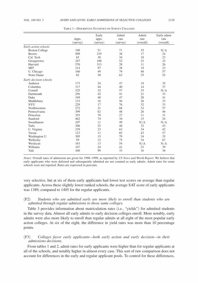
We consider the aggregated data for the set of 28 colleges that received early applications from more than ten survey participants. Table 1 lists the colleges along with summary statistics. Applicants from the survey were admitted at significantly higher rates than the aggregate rates for the entire applicant pool at each college, as one would expect given the survey design. A total of 2,376 survey participants applied to at least one of these 28 colleges, and 1,354 (57.8 percent) of these participants applied early to at least one of these colleges. These 28 colleges received a total of 7,243 applications from survey participants.
We base our analysis on several numerical measures. We use the recentered scale for SAT-1 scores, which include one mathematics score and one verbal score, with each score ranging from 200 to 800. In addition, survey respondents listed their three most significant accomplishments to provide a feel for extracurricular activities. We categorized these accomplishments in terms of attractiveness to college admissions officers on a 1 to 5 scale, with 5 as the most desirable and 1 the least. This student activity rating serves as a proxy for an admissions office rating. An experi-enced college admissions officer classified the quality of the high schools that participated in the survey on a similar 1 to 5 scale.
(F1) At the very top schools, early applicants have stronger test scores on average than regular applicants. At schools just below the very top, early applicants tend to have lower test scores on average than regular applicants.
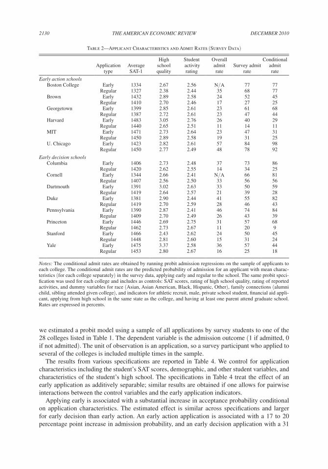
Table 2 presents detailed statistics for the 14 individual colleges that received early appli-cations from more than 30 survey participants. The five top-ranked schools are Harvard, Yale, Princeton, Stanford, and MIT. At four of these schools, early applicants had higher SAT scores on average than regular applicants. Across these schools, the average SAT score of early appli-cants was 1468, compared to 1450 for regular applicants. The remaining nine schools are also
7 In addition to Harvard, Princeton, Yale, and Stanford, the remaining two schools are MIT and Caltech.8 The College Admission Project was run jointly by Avery and Hoxby. AFZ report similar qualitative findings consis-
tent with stylized facts (F1) through (F5) in their analysis of applicant-level data (including admission ratings) provided by admissions offices at 14 selective colleges.
VOL. 100 NO. 5 2129AVERY AND LEVIN: EARLY ADmISSIONS AT SELEcTIVE cOLLEgES
very selective, but at six of them early applicants had lower test scores on average than regular applicants. Across these slightly lower ranked schools, the average SAT score of early applicants was 1389, compared to 1405 for the regular applicants.
(F2) Students who are admitted early are more likely to enroll than students who are admitted through regular admissions to those same colleges.
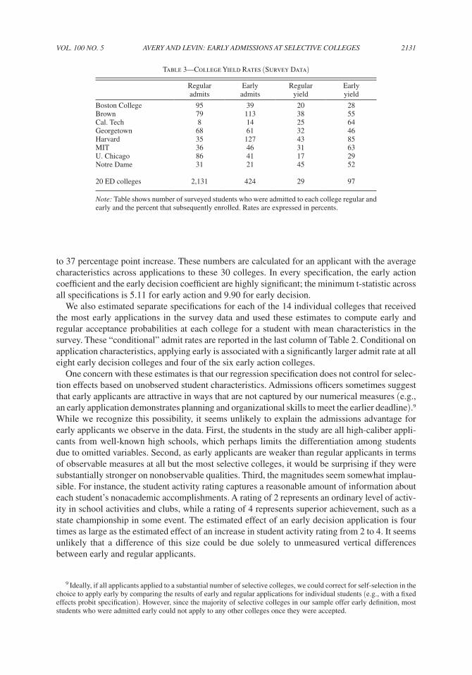
Table 3 provides information about matriculation rates (i.e., “yields”) for admitted students in the survey data. Almost all early admits to early decision colleges enroll. More notably, early admits were also more likely to enroll than regular admits at all eight of the most popular early action colleges. At six of the eight, the difference in yield rates was more than 10 percentage points.
(F3) colleges favor early applicants—both early action and early decision—in their admissions decisions.
From tables 1 and 2, admit rates for early applicants were higher than for regular applicants at all of the schools, and notably higher in almost every case. This sort of raw comparison does not account for differences in the early and regular applicant pools. To control for these differences,
Table 1—Descriptive Statistics on Survey Colleges
Apps. (survey)
Early apps.
(survey)
Admit rate
(survey)
Admit rate
(overall)
Early admit rate
(overall)Early action schools
Boston College 190 51 71 35 N/ABrown 509 219 38 17 24Cal. Tech 65 30 34 18 23Georgetown 247 100 52 23 23Harvard 570 313 28 11 26MIT 214 97 38 19 23U. Chicago 160 49 79 48 57Notre Dame 82 30 63 35 52
Early decision schoolsAmherst 173 24 47 19 35Columbia 317 44 40 14 37Cornell 325 32 57 33 N/ADartmouth 256 42 41 21 33Duke 349 40 47 28 41Middlebury 133 16 56 26 33NYU 229 17 76 32 33Northwestern 272 21 68 32 57Pennsylvania 399 62 48 26 46Princeton 355 70 27 11 31Stanford 462 74 34 15 24Swarthmore 107 11 49 N/A N/ATufts 306 25 48 32 43U. Virginia 239 23 63 34 42Vassar 123 11 65 43 57Washington U. 305 15 79 34 35Wellesley 59 12 75 34 67Wesleyan 163 13 54 N/A N/AWilliams 167 24 41 23 39Yale 440 99 33 16 36
Notes: Overall rates of admission are given for 1998–1999, as reported by US News and World Report. We believe that early applicants who were deferred and subsequently admitted are not counted as early admits. Admit rates for some schools were not reported. Rates are expressed in percents.
DEcEmBER 20102130 THE AmERIcAN EcONOmIc REVIEW
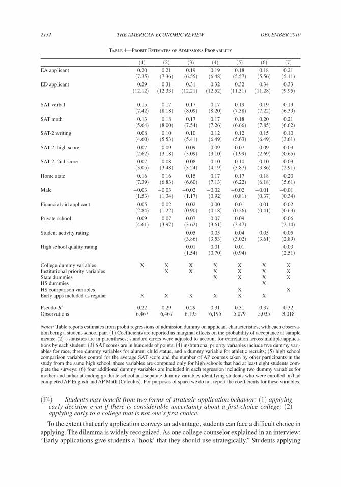
we estimated a probit model using a sample of all applications by survey students to one of the 28 colleges listed in Table 1. The dependent variable is the admission outcome (1 if admitted, 0 if not admitted). The unit of observation is an application, so a survey participant who applied to several of the colleges is included multiple times in the sample.
The results from various specifications are reported in Table 4. We control for application characteristics including the student’s SAT scores, demographic, and other student variables, and characteristics of the student’s high school. The specifications in Table 4 treat the effect of an early application as additively separable; similar results are obtained if one allows for pairwise interactions between the control variables and the early application indicators.
Applying early is associated with a substantial increase in acceptance probability conditional on application characteristics. The estimated effect is similar across specifications and larger for early decision than early action. An early action application is associated with a 17 to 20 percentage point increase in admission probability, and an early decision application with a 31
Table 2—Applicant Characteristics and Admit Rates (Survey Data)
Application type
Average SAT-1
High school quality
Student activity rating
Overall admit rate
Survey admit rate
Conditional admitrate
Early action schoolsBoston College Early 1334 2.67 2.56 N/A 77 77
Regular 1327 2.38 2.44 35 68 77Brown Early 1432 2.89 2.58 24 52 45
Regular 1410 2.70 2.46 17 27 25Georgetown Early 1399 2.85 2.61 23 61 68
Regular 1387 2.72 2.61 23 47 44Harvard Early 1483 3.05 2.76 26 40 29
Regular 1440 2.65 2.51 11 14 11MIT Early 1471 2.73 2.64 23 47 31
Regular 1450 2.89 2.58 19 31 25U. Chicago Early 1423 2.82 2.61 57 84 98
Regular 1450 2.77 2.49 48 78 92
Early decision schoolsColumbia Early 1406 2.73 2.48 37 73 86
Regular 1420 2.62 2.55 14 34 25Cornell Early 1344 2.66 2.41 N/A 66 81
Regular 1407 2.56 2.50 33 56 56Dartmouth Early 1391 3.02 2.63 33 50 59
Regular 1419 2.64 2.57 21 39 28Duke Early 1381 2.90 2.44 41 55 82
Regular 1419 2.70 2.59 28 46 43Pennsylvania Early 1390 2.87 2.41 46 74 84
Regular 1409 2.70 2.49 26 43 39Princeton Early 1446 2.69 2.75 31 57 68
Regular 1462 2.73 2.67 11 20 9Stanford Early 1466 2.43 2.62 24 50 45
Regular 1448 2.81 2.60 15 31 24Yale Early 1475 3.37 2.58 36 57 44
Regular 1453 2.80 2.67 16 25 18
Notes: The conditional admit rates are obtained by running probit admission regressions on the sample of applicants to each college. The conditional admit rates are the predicted probability of admission for an applicant with mean charac-teristics (for each college separately) in the survey data, applying early and regular to the school. The same probit speci-fication was used for each college and includes as controls: SAT scores, rating of high school quality, rating of reported activities, and dummy variables for race (Asian, Asian American, Black, Hispanic, Other), family connections (alumni child, sibling attended given college), and indicators for athletic recruit, male, private school student, financial aid appli-cant, applying from high school in the same state as the college, and having at least one parent attend graduate school. Rates are expressed in percents.
VOL. 100 NO. 5 2131AVERY AND LEVIN: EARLY ADmISSIONS AT SELEcTIVE cOLLEgES
to 37 percentage point increase. These numbers are calculated for an applicant with the average characteristics across applications to these 30 colleges. In every specification, the early action coefficient and the early decision coefficient are highly significant; the minimum t-statistic across all specifications is 5.11 for early action and 9.90 for early decision.
We also estimated separate specifications for each of the 14 individual colleges that received the most early applications in the survey data and used these estimates to compute early and regular acceptance probabilities at each college for a student with mean characteristics in the survey. These “conditional” admit rates are reported in the last column of Table 2. Conditional on application characteristics, applying early is associated with a significantly larger admit rate at all eight early decision colleges and four of the six early action colleges.
One concern with these estimates is that our regression specification does not control for selec-tion effects based on unobserved student characteristics. Admissions officers sometimes suggest that early applicants are attractive in ways that are not captured by our numerical measures (e.g., an early application demonstrates planning and organizational skills to meet the earlier deadline).9 While we recognize this possibility, it seems unlikely to explain the admissions advantage for early applicants we observe in the data. First, the students in the study are all high-caliber appli-cants from well-known high schools, which perhaps limits the differentiation among students due to omitted variables. Second, as early applicants are weaker than regular applicants in terms of observable measures at all but the most selective colleges, it would be surprising if they were substantially stronger on nonobservable qualities. Third, the magnitudes seem somewhat implau-sible. For instance, the student activity rating captures a reasonable amount of information about each student’s nonacademic accomplishments. A rating of 2 represents an ordinary level of activ-ity in school activities and clubs, while a rating of 4 represents superior achievement, such as a state championship in some event. The estimated effect of an early decision application is four times as large as the estimated effect of an increase in student activity rating from 2 to 4. It seems unlikely that a difference of this size could be due solely to unmeasured vertical differences between early and regular applicants.
9 Ideally, if all applicants applied to a substantial number of selective colleges, we could correct for self-selection in the choice to apply early by comparing the results of early and regular applications for individual students (e.g., with a fixed effects probit specification). However, since the majority of selective colleges in our sample offer early definition, most students who were admitted early could not apply to any other colleges once they were accepted.
Table 3—College Yield Rates (Survey Data)
Regular admits
Early admits
Regular yield
Early yield
Boston College 95 39 20 28Brown 79 113 38 55Cal. Tech 8 14 25 64Georgetown 68 61 32 46Harvard 35 127 43 85MIT 36 46 31 63U. Chicago 86 41 17 29Notre Dame 31 21 45 52
20 ED colleges 2,131 424 29 97
Note: Table shows number of surveyed students who were admitted to each college regular and early and the percent that subsequently enrolled. Rates are expressed in percents.
DEcEmBER 20102132 THE AmERIcAN EcONOmIc REVIEW
(F4) Students may benefit from two forms of strategic application behavior: (1) applying early decision even if there is considerable uncertainty about a first-choice college; (2) applying early to a college that is not one’s first choice.
To the extent that early application conveys an advantage, students can face a difficult choice in applying. The dilemma is widely recognized. As one college counselor explained in an interview: “Early applications give students a ‘hook’ that they should use strategically.” Students applying
Table 4—Probit Estimates of Admissions Probability
(1) (2) (3) (4) (5) (6) (7)EA applicant 0.20 0.21 0.19 0.19 0.18 0.18 0.21
(7.35) (7.36) (6.55) (6.48) (5.57) (5.56) (5.11)ED applicant 0.29 0.31 0.31 0.32 0.32 0.34 0.33
(12.12) (12.33) (12.21) (12.52) (11.31) (11.28) (9.95)
SAT verbal 0.15 0.17 0.17 0.17 0.19 0.19 0.19(7.42) (8.18) (8.09) (8.20) (7.38) (7.22) (6.39)
SAT math 0.13 0.18 0.17 0.17 0.18 0.20 0.21(5.64) (8.00) (7.54) (7.26) (6.66) (7.85) (6.62)
SAT-2 writing 0.08 0.10 0.10 0.12 0.12 0.15 0.10(4.60) (5.53) (5.41) (6.49) (5.63) (6.49) (3.61)
SAT-2, high score 0.07 0.09 0.09 0.09 0.07 0.09 0.03(2.62) (3.18) (3.09) (3.10) (1.99) (2.69) (0.65)
SAT-2, 2nd score 0.07 0.08 0.08 0.10 0.10 0.10 0.09(3.05) (3.48) (3.24) (4.19) (3.87) (3.86) (2.91)
Home state 0.16 0.16 0.15 0.17 0.17 0.18 0.20(7.39) (6.83) (6.60) (7.13) (6.22) (6.18) (5.61)
Male −0.03 −0.03 −0.02 −0.02 −0.02 −0.01 −0.01(1.53) (1.34) (1.17) (0.92) (0.81) (0.37) (0.34)
Financial aid applicant 0.05 0.02 0.02 0.00 0.01 0.01 0.02(2.84) (1.22) (0.90) (0.18) (0.26) (0.41) (0.63)
Private school 0.09 0.07 0.07 0.07 0.09 0.06(4.61) (3.97) (3.62) (3.61) (3.47) (2.14)
Student activity rating 0.05 0.05 0.04 0.05 0.05(3.86) (3.53) (3.02) (3.61) (2.89)
High school quality rating 0.01 0.01 0.01 0.03(1.54) (0.70) (0.94) (2.51)
College dummy variables X X X X X X XInstitutional priority variables X X X X X XState dummies X X X XHS dummies XHS comparison variables X XEarly apps included as regular X X X X X X
Pseudo-R2 0.22 0.29 0.29 0.31 0.31 0.37 0.32Observations 6,467 6,467 6,195 6,195 5,079 5,035 3,018
Notes: Table reports estimates from probit regressions of admission dummy on applicant characteristics, with each observa-tion being a student-school pair. (1) Coefficients are reported as marginal effects on the probability of acceptance at sample means; (2) t-statistics are in parentheses; standard errors were adjusted to account for correlation across multiple applica-tions by each student; (3) SAT scores are in hundreds of points; (4) institutional priority variables include five dummy vari-ables for race, three dummy variables for alumni child status, and a dummy variable for athletic recruits; (5) high school comparison variables control for the average SAT score and the number of AP courses taken by other participants in the study from the same high school: these variables are computed only for high schools that had at least eight students com-plete the surveys; (6) four additional dummy variables are included in each regression including two dummy variables for mother and father attending graduate school and separate dummy variables identifying students who were enrolled in/had completed AP English and AP Math (Calculus). For purposes of space we do not report the coefficients for these variables.
VOL. 100 NO. 5 2133AVERY AND LEVIN: EARLY ADmISSIONS AT SELEcTIVE cOLLEgES
early decision have a particularly acute trade-off because they must weigh the admissions advan-tage against the potential cost of premature commitment. Avery, Fairbanks, and Zeckhauser found that in retrospective interviews, less than two-thirds of students who applied early and were attending early decision colleges had a strong preference for that college at the time that they applied.
A further complication is that for a given student, the benefit of early application may vary across colleges. For example, a student who is substantially below or above the bar for admission at a given college will not get an admissions benefit from applying early. Instead, early applica-tion is likely to be most efficacious at a college where the student is competitive but not certain (or possibly not likely) to be admitted as a regular applicant. As a result, it frequently may be optimal for a student to apply early to a second or lower choice college rather than to a long-shot first-choice college. Again, this situation seems to be well understood. As another college coun-selor explained: “If you are willing to lower expectation one rung lower, you might be able to get better outcomes [by applying early].”
(F5) Early action is disproportionately used by the highest ranked schools, whereas lower ranked schools typically use early decision.
This last stylized fact relates to the use of early admissions programs by different institutions, and we have already mentioned the evidence. Of the top six schools in the US News rankings, four offer early action and none offers early decision. Of the remaining 32 “most selective” schools, 21 offer early decision and only five offer early action.
II. An Illustrative Example
We first describe a numerical example that illustrates the model and its relationship to the empirical evidence. There are two selective schools, A and B, and a third college C that admits all applicants. There is a unit mass of students. Each student is described by an ability v and a taste parameter y. We assume for now that ability and taste are independently distributed. Student abilities are uniformly distributed on [0, 1] and tastes are uniform on [−1/3, 2/3].
A student’s taste parameter reflects her school preference: a higher y means the student is more enthusiastic about school A. For this example, assume that a student with taste y obtains a payoff 1 + ay from attending school A, a payoff 1 −by from attending school B, and zero from attend-ing school C. With a, b > 0, students with positive y prefer A to B, meaning that the majority of students prefer A. We assume that a = 48/7 and b = 6/7. 10
The schools prefer high ability students but also students who are eager to attend. Suppose that A places a value v + αy on a student of type (v, y), while B’s value is v −αy, where α = 1/3. Each selective school wants to enroll K = 1/3 of the students. The schools set their admission policies to maximize the average value of their enrolled students, while aiming for an enrollment of K. In equilibrium, both schools will hit their enrollment target exactly.
An important feature we want to capture is that students and schools each have some of the relevant information about a given match. We incorporate this by assuming the schools can assess a student’s ability v, but not her preference y, while each student knows her preference y but not v. Below we consider what happens if each student has an imperfect signal of her v.
10 Our model in the next section assumes that students always view C as their third choice. In this example, a student with y < −7/48 actually prefers C to A, but this is unimportant because students with y < 0 are never admitted to A unless they are also admitted to their first choice, B. The example would work out the same if students with y ≤ 0 all had a payoff of 1 from attending A, so that C was everyone’s third choice.
DEcEmBER 20102134 THE AmERIcAN EcONOmIc REVIEW
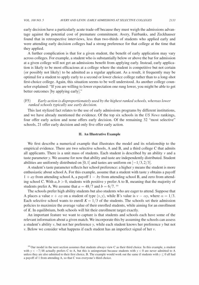
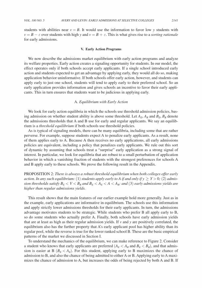
Regular Admissions.—If there are no early admissions, students apply to both selective schools. In equilibrium, A admits all students with abilities above A = 1/2, and B admits stu-dents with abilities above B = 1/3. Students with abilities above A are admitted to both schools. Those with y ≥0 enroll at A and those with y < 0 enroll at B. The equilibrium admission and enrollment patterns are shown in Figure 1. The admission thresholds are an equilibrium in the sense that given B’s policy, A gets the best students it can while meeting its target enrollment, and the same is true for B given A’s policy. In equilibrium, B must use a lower threshold because most of the top students choose A when given the choice.
Early Action.—With early action, each student can designate one application as an early appli-cation, and the schools can use different thresholds for early and regular applicants. Recall that early action is nonbinding, so that a student admitted early can still choose to go elsewhere.
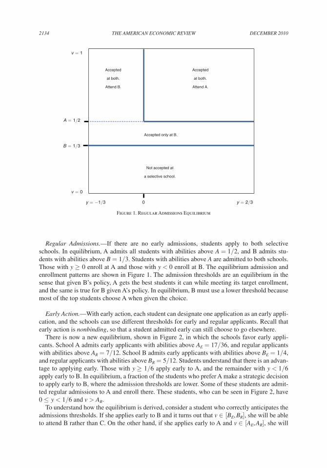
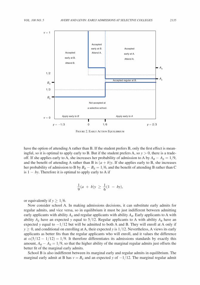
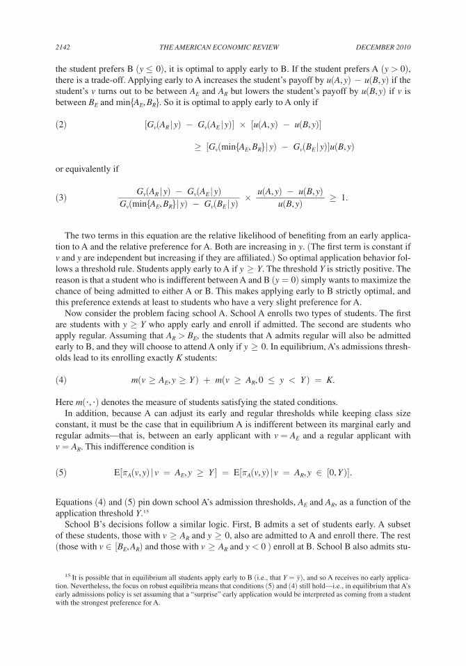
There is now a new equilibrium, shown in Figure 2, in which the schools favor early appli-cants. School A admits early applicants with abilities above AE = 17/36, and regular applicants with abilities above AR = 7/12. School B admits early applicants with abilities above BE = 1/4, and regular applicants with abilities above BR = 5/12. Students understand that there is an advan-tage to applying early. Those with y ≥1/6 apply early to A, and the remainder with y < 1/6 apply early to B. In equilibrium, a fraction of the students who prefer A make a strategic decision to apply early to B, where the admission thresholds are lower. Some of these students are admit-ted regular admissions to A and enroll there. These students, who can be seen in Figure 2, have 0 ≤y < 1/6 and v > AR.
To understand how the equilibrium is derived, consider a student who correctly anticipates the admissions thresholds. If she applies early to B and it turns out that v ∈[BE, BR], she will be able to attend B rather than C. On the other hand, if she applies early to A and v ∈[AE, AR], she will
Figure 1. Regular Admissions Equilibrium
v = 1
0
Accepted only at B.
Accepted
at both.
Attend A.
Not accepted at
a selective school.
A = 1/2
B = 1/3
Accepted
at both.
Attend B.
v = 0
y = 2/3 y = −1/3
VOL. 100 NO. 5 2135AVERY AND LEVIN: EARLY ADmISSIONS AT SELEcTIVE cOLLEgES
have the option of attending A rather than B. If the student prefers B, only the first effect is mean-ingful, so it is optimal to apply early to B. But if the student prefers A, so y > 0, there is a trade-off. If she applies early to A, she increases her probability of admission to A by AR −AE = 1/9, and the benefit of attending A rather than B is (a + b)y. If she applies early to B, she increases her probability of admission to B by BR −BE = 1/6, and the benefit of attending B rather than C is 1 −by. Therefore it is optimal to apply early to A if
1 _9 (a + b)y ≥ 1 _
6 (1 − by),
or equivalently if y ≥1/6.Now consider school A. In making admissions decisions, it can substitute early admits for
regular admits, and vice versa, so in equilibrium it must be just indifferent between admitting early applicants with ability AE and regular applicants with ability AR. Early applicants to A with ability AE have an expected y equal to 5/12. Regular applicants to A with ability AR have an expected y equal to −1/12 but will be admitted to both A and B. They will enroll at A only if y ≥0, and conditional on enrolling at A, their expected y is 1/12. Nevertheless, A views its early applicants as better fits than the regular applicants who will enroll, and it values the difference at α(5/12 −1/12) = 1/9. It therefore differentiates its admissions standards by exactly this amount, AR −AE = 1/9, so that the higher ability of the marginal regular admits just offsets the better fit of the marginal early admits.
School B is also indifferent between its marginal early and regular admits in equilibrium. The marginal early admit at B has v = BE and an expected y of −1/12. The marginal regular admit
Figure 2. Early Action Equilibrium
Not accepted at
a selective school.
0
BE
AR
Accepted
early at B.
Attend B.
Accepted
early at A.
Attend A.
Accepted regular at B.
Accepted
early at B.
Attend A.
1/6
BR
AE
Apply early to AApply early to B
y = −1/3 y = 2/3
v = 1
1/2
1/3
v = 0
DEcEmBER 20102136 THE AmERIcAN EcONOmIc REVIEW
has v = BR and an expected y of 5/12. School B places a value α(5/12 + 1/12) = 1/6 on the better fit of the marginal early admit and differentiates its admissions thresholds by this same amount: BR −BE = 1/6. Given that students apply early to A if y ≥1/6, that AR −AE = 1/9 and BR −BE = 1/6, and that each school must enroll 1/3 of the students in equilibrium, it is possible to solve for the equilibrium values of AR, AE, BR, and BE. Indeed it is easy to calculate using Figure 2 and the stated thresholds that both schools exactly hit their enrollment targets.
Features of the Equilibrium.—The equilibrium has a number of features that correspond to the discussion in the previous section, and that are shared by our more general model.
First, in equilibrium an early application conveys a credible message that a student is enthu-siastic about a school and likely to enroll. The schools use this information in equilibrium and favor their early applicants.
Second, students have an incentive to be strategic and may not apply early to their preferred school. In particular, only students who are sufficiently enthusiastic about A risk an early appli-cation. One way to understand this is that although applying early to A raises the odds of being accepted, it also means not applying early to B. This creates an additional risk of missing out on both A and B. The fact that students are uncertain about where they will be accepted also means that some students regret their early application decision. A student who strategically applied to B may regret not taking a chance on A, while some students who applied early to A and were rejected may regret not applying early to B.
Despite student strategizing, however, the equilibrium makes both schools better off than they were with regular admissions. In our example, the average value that A places on its students increases from 31/36 with regular admissions to 373/432 with early admissions, and B’s aver-age value increases from 7/12 to 173/288. We show below that this is a general property of the model. Intuitively, early applications provide additional information that allows schools to sort the students based on fit. What makes this welfare-enhancing for the schools is that their prefer-ences regarding fit are aligned. Holding fixed the average v at each school, both schools prefer to see high y students enroll at A, and low y students enroll at B.
Student welfare is less straightforward. From an ex post perspective, some students do worse in the early action equilibrium than with regular admissions. For instance, students with y ∈[0, 1/6) and v ∈[1/2, AR) prefer A and end up there with regular admissions, but with early action apply early to B and end up enrolling there. Nevertheless, from an ex ante perspective, the students are arguably better off with early action. The average student utility increases, and in fact, in this example the distribution of realized student utilities increases in the sense of first-order stochastic dominance. This turns out to be a reasonably general property of the model.
One caveat relates to equilibrium selection. Signaling games often have many equilibria, and so it is natural to ask if the equilibrium we have described is a sensible one. So long as the schools interpret a “surprise” early application as an indication of enthusiasm, all early action equilibria will share these same qualitative features. In fact, subject to this refinement, the equilibrium we have described in this example is unique.
Early Decision.—The model can also be used to analyze the effect of binding early decision poli-cies. The early decision equilibrium is similar to the early action case, with one notable difference. Students admitted early to B are unable to later enroll at A. All else equal, this raises the cost of a strategic early application to B. A second difference in the context of our model is that if B uses early decision, A’s early admissions policy becomes irrelevant for the equilibrium outcome.
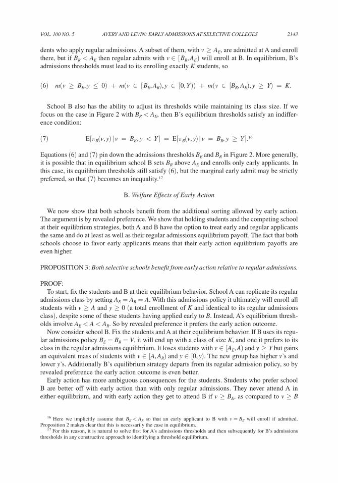
To see this, consider the case where B offers early decision and A has only regular admissions. The equilibrium is depicted in Figure 3. Students with y < Y = 0.039 apply early to school B, which uses thresholds BE = 0.229 and BR = 0.229 for its early and regular applicants. School A

VOL. 100 NO. 5 2137AVERY AND LEVIN: EARLY ADmISSIONS AT SELEcTIVE cOLLEgES
sets an admissions threshold A = 0.497. The student application decision is similar to the early action case. Students with y ≤0 have a clear preference for applying early to B. Students with y > 0 have a trade-off. An early application to B means that if v ∈[BE, BR), they get to attend B rather than C, but it also means that if v ≥A, they are compelled to attend B rather than going to A. The stronger the preference for A, the less attractive it is to apply early to B, and the cutoff preference is y = Y.
On the school side, A’s admissions decision is very simple. Taking application behavior as given, it chooses its threshold to attract exactly 1/3 of the students. School B has a more com-plicated decision because it has to account for the better fit of the early applicants. Its early applicants have an expected y of −0.147. Its regular applicants have an expected y of 0.353. School B values the difference at α(0.353 + 0.147) = 1/6. As a result, it sets its thresholds so that BR −BE = 1/6, and of course, so that it hits its enrollment target of 1/3.11
Although the equilibrium has similar features to the early action equilibrium, the welfare prop-erties are different. In this particular example, both A and B benefit from early decision relative to regular admissions. But we show later in the paper that this is not always the case. School B always benefits from introducing early decision, but A can be harmed if enough high ability can-didates are strategic in the application process and end up at B.
11 Derivations of the thresholds are in the online Appendix. To see why an early admission process for A would make no difference, note that the relevant students for A are those who do not apply early to B (the ones who apply early to B either are admitted and locked in, or have abilities too low to be interesting to A). So if A introduced early admissions and favored these applicants, it immediately would attract all the students who weren’t applying early to B and would end up using the same admissions threshold A to fill its class.
Figure 3. Early Decision Equilibrium
Not accepted at
a selective school.
0
Accepted
early at B.
Attend B.
Accepted
regular at A.
Attend A.
Accepted regular at B.
Y
A
Apply early to AApply early to B
BE
BR
y = −1/3 y = 2/3
v = 1
1/2
1/3
v = 0
DEcEmBER 20102138 THE AmERIcAN EcONOmIc REVIEW
Better informed students.—So far in our example, students are uninformed about their ability at the time they apply. In reality, most students have some idea of where they are likely to be admit-ted. Incorporating this leads to an equilibrium in which A attracts early admissions from somewhat better qualified students, while the converse is true for B, matching the empirical pattern described in Section IB.
To keep things simple, suppose that each student observes an informative signal equal to either g or b. Half the students observe a g and half a b. Students who observe g have abilities distrib-uted on [0, 1] with density 2x. Students who observe b have abilities distributed on [0, 1] with density 2(1 −x). So the population distribution of ability is still uniform, but students with a g signal are on average higher ability. For simplicity, we assume the schools continue to observe each applicant’s ability v, but don’t observe whether the applicant’s signal is g or b.
The additional information has no effect on the regular admissions equilibrium. Students still apply to both schools, the schools still base admissions on the ability v, and the students still make decisions on the basis of their taste y. Early admissions, however, work differently. In the new early action equilibrium, students with a g signal apply early to A if y≥0.114, while stu-dents with b signals apply early to A only if y≥0.226. The schools still set different admissions thresholds for early and late applicants. For the specific parameters we’ve chosen, the equilib-rium thresholds are only slightly adjusted: AE = 0.473, AR = 0.580, BE = 0.252, and BR = 0.416. Figure 4 shows the new equilibrium.
The new feature of the equilibrium is that students with good test scores (i.e., a g signal) are more likely to apply early to A. The reason is that these students assign relatively high prob-ability to having abilities in the range [AE, AR ] compared to [BE, BR ]. An implication is that A’s early applicants look somewhat stronger than its regular applicants, while the converse is true at B. We observed this pattern—the most selective schools having particularly strong early applicants—in Section IB. The implications of the different application behavior show up in regions 1 and 2 of Figure 4. Students in Region 1 who had a g signal end up at school A, hav-ing applied early, while students in the same region with a b signal end up at B. At the same time, students in Region 2 who had a g signal end up at C, while students in the same region with a b signal end up at B. So in these two regions, otherwise identical students with differ-ent private signals of ability choose different early application strategies and ultimately attend different colleges.
III. The Model
We now extend the example into a more general model. The building blocks are the same: stu-dents are differentiated both in their academic ability and in their “fit” for different schools, and early admission programs allow schools to identify enthusiastic students. Again we assume there is a population of students of unit measure, and three schools, A, B, and C. Schools A and B each want to enroll exactly K students, where K < 1/2. School C accepts all applicants.
Each student is described by an ability v and a taste parameter y that indicates the student’s preference. Students with high y are enthusiastic about A; students with low y are enthusiastic about B. Letting u(s, y) be the utility that a student with taste y obtains from attending school s, we assume that u(A, y), u(B, y) are continuous in y and strictly positive, and that u(A, y)/u(B, y) is increasing in y and crosses one at y = 0. We also assume that u(c, y) = 0, so that students all prefer to attend a selective school.
Student types (v, y) in the population are distributed on the rectangle ×, with an atomless distribution g. We assume that students generally favor A over B, making A the more selective or “higher ranked” school. In our notation, gy(0|v)∈(0, 1/2), so at any ability level v more than half the students have y≥0 and prefer A. In the example above, we assumed ability and taste

VOL. 100 NO. 5 2139AVERY AND LEVIN: EARLY ADmISSIONS AT SELEcTIVE cOLLEgES
were independent. Here we weaken that assumption by allowing v and y to be affiliated, so that high-ability students may have a particular preference for school A.12
We denote the values that schools A and B assign to a student with characteristics (v, y) as πA(v, y) and πB(v, y). Both schools like high academic ability and also students who are good fits. So πA is increasing in (v, y) and πB is increasing in (v, −y). Each school tries to maximize the average value of its students while hitting its enrollment target K. One subtlety here is that if v and y are positively correlated, higher ability students are on average more enthusiastic about A. To ensure this correlation does not lead B to prefer low ability students, we assume Ey[πB(v, y)|v, y ∈Ω] is increasing in v for any set Ω⊂.13 For future reference, we also define V so that 1 − gv(V ) = 2K. That is, V is the ability threshold such that if all students with v≥V were to divide equally between the selective schools, the schools would both enroll K students.
Early applications can play a role in signaling student preferences when the information required to implement an efficient match between students and colleges is dispersed. In our baseline model, we assume a clean separation of information. Students know their preferences at the time they apply, but not how colleges will assess their academic ability (i.e., each student knows her y, but not her v). Later we will show that our results carry through even if students have imperfect information about v. In contrast, each school can assess the academic ability of applicants accurately (i.e., each student’s v) but cannot infer enthusiasm (y) directly from a
12 Affiliation is a strong version of positive correlation. A distribution g satisfies affiliation if its density g has the property that f (v′, y′)f (v, y)≥f (v′, y)f (v, y′) for any v′ > v and y′ > y, which means that a higher v is relatively more likely among students with a higher y.
13 This condition says that if a school B could choose between two students with abilities v′ and v, and v′ > v, and had the same information about the taste of each student (i.e., that they had y’s in some interval), it would prefer the higher ability student. This is immediate if v and y are independent and holds under affiliation provided school B places sufficient weight on student ability.
Figure 4. Early Action with Informed Students
Not accepted ata selective school.
0
Accepted
early at B.
Attend B.
Accepted
early at A.
Attend A.
Accepted at B. Attend B.
Accepted
early at A
or B.
Attend A.
Apply early to B Apply early to A
Region1
Region
2
Apply early to A if g
0.2260.114
BE
AR
BR
AE
y = −1/3 y = 2/3
v = 1
1/2
1/3
v = 0
DEcEmBER 20102140 THE AmERIcAN EcONOmIc REVIEW
student’s application. Of course if v, y are correlated, knowledge of one of these values may pro-vide some information about the other.
Throughout the paper, we consider the following admissions game. Colleges first announce if they will offer early admissions. Students then submit applications and can potentially desig-nate one application as an “early” application. We assume the cost of submitting applications is negligible, so that students find it optimal to apply everywhere.14 The schools then make their admission decisions, and finally students choose among the colleges where they were admitted. Naturally students enroll at their preferred school, except that a student admitted early decision must enroll at that school. We analyze equilibria of this game in which the colleges cannot com-mit in advance to favoring (or disfavoring) early applicants by any particular amount. This focus rules out the possibility that a school would seek to influence applicant decisions by precommit-ting to a specific admissions rule that is subsequently suboptimal. Such behavior might benefit a school in theory but seems inconsistent with the actual operation of the market.
IV. Regular Admissions Equilibrium
Suppose the schools offer only regular admissions. Each student will apply to all three col-leges. The selective schools choose their admissions policies to maximize their expected payoff subject to the constraint that they expect to enroll K students. There is a unique equilibrium in which each school uses a threshold policy for admissions. School A admits all students with v≥A and school B admits all students with v≥B, where A > B. Students with ability above A are admitted at both schools. Of these students, the majority enroll at A. The threshold A is set so that the mass of students with y≥0 and v≥A (denoted m(v≥A, y≥0)) just equals K. School B also admits students with abilities between A and B. Its admission threshold B must equal V because all students with abilities v≥B will enroll at one of the selective schools and their numbers must total 2K.
PROPOSITION 1: There is a unique equilibrium in which students apply to all schools and the schools use admission thresholds A, B with m(v≥A, y≥0) = K, and B = V < A.
Proposition 1 rules out the possibility of an equilibrium in which the schools use something other than threshold admissions policies. These equilibria can exist in a limiting “symmetric” case of our model where v and y are independent and gy(0) = 1/2. In this case, exactly half the students prefer A to B, and there can be equilibria in which the schools use identical admissions policies but admit some students with v < V and reject others with v > V. The explanation for these equilibria is that each school benefits from admitting students who are also admitted at the other school. Students admitted at both schools self-select on the basis of fit, and the schools benefit from this self-selection. The nonthreshold equilibria involve a coordination failure: the schools would be better off using threshold policies, but neither school individually wants to adopt one. The proof of Proposition 1 shows that this type of coordination failure cannot occur with even a bit of hierarchy between the schools.
This discussion, however, highlights an important feature of the model. In the regular admis-sions equilibrium, the highest ranked students, with abilities v≥A, self-select into their pre-ferred college. So even without an explicit signaling opportunity such as an early application, equilibrium involves some preference-based sorting. Nevertheless, it is clear that the schools would like to have additional information. For instance, suppose B knows the preferences of
14 The problem of application costs, and the issues they raise for early admissions, has been studied by Hector Chade, Greg Lewis, and Lones Smith (2010) and Yuan-Chuan Lien (2009).
VOL. 100 NO. 5 2141AVERY AND LEVIN: EARLY ADmISSIONS AT SELEcTIVE cOLLEgES
students with abilities near v = B. It would use the information to favor low y students with v = B − ε over students with high y and v = B +ε. This is what gives rise to a sorting rationale for early admissions.
V. Early Action Programs
We now describe the admissions market equilibrium with early action programs and analyze its welfare properties. Early action creates a signaling opportunity for students. In our model, the effect operates only if both schools accept early applicants. If a single school introduced early action and students expected to get an advantage by applying early, they would all do so, making application behavior uninformative. If both schools offer early action, however, and students can apply early to just one school, students will tend to apply early to their preferred school. So an early application provides information and gives schools an incentive to favor their early appli-cants. This in turn ensures that students want to be judicious in applying early.
A. Equilibrium with Early Action
We look for early action equilibria in which the schools use threshold admission policies, bas-ing admission on whether student ability is above some threshold. Let AE, AR and BE, BR denote the admissions thresholds that A and B use for early and regular applicants. We say an equilib-rium is a threshold equilibrium if both schools use threshold policies.
As is typical of signaling models, there can be many equilibria, including some that are rather perverse. For example, suppose students expect A to penalize early applicants. As a result, none of them applies early to A. Because A then receives no early applications, all early admissions policies are equivalent, including a policy that penalizes early applicants. We rule out this sort of dynamic by assuming that schools treat a “surprise” early application as a strong signal of interest. In particular, we look for equilibria that are robust to a small perturbation of application behavior in which a vanishing fraction of students with the strongest preferences for schools A and B apply early to these schools. We prove the following result in the Appendix.
PROPOSITION 2: There is always a robust threshold equilibrium when both colleges offer early action. In any such equilibrium: (1) students apply early to A if and only if y≥Y > 0; (2) admis-sion thresholds satisfy BE < V < BR and BE < AE < A < AR; and (3) early admissions yields are higher than regular admissions yields.
This result shows that the main features of our earlier example hold more generally. Just as in the example, early applications are informative in equilibrium. The schools use this information and apply strictly lower admissions thresholds for their early applicants. In turn, the admissions advantage motivates students to be strategic. While students who prefer B all apply early to B, so do some students who actually prefer A. Finally, both schools have early admission yields that are at least as high as their regular admission yields. If v and y are positively correlated, the equilibrium also has the further property that A’s early applicant pool has higher ability than its regular pool, while the reverse is true for the lower ranked school B. These are the basic empirical patterns of the market we discussed in Section I.
To understand the mechanics of the equilibrium, we can make reference to Figure 2. Consider a student who knows that early applicants are preferred (AE < AR and BE < BR), and that admis-sion is easier at B (BE < AE). For this student, applying early to B maximizes the chance of admission to B, and also the chance of being admitted to either A or B. Applying early to A maxi-mizes the chance of admission to A, but increases the odds of being rejected by both A and B. If
DEcEmBER 20102142 THE AmERIcAN EcONOmIc REVIEW
the student prefers B (y ≤0), it is optimal to apply early to B. If the student prefers A (y > 0), there is a trade-off. Applying early to A increases the student’s payoff by u(A, y)−u(B, y) if the student’s v turns out to be between AE and AR but lowers the student’s payoff by u(B, y) if v is between BE and min{AE, BR}. So it is optimal to apply early to A only if
(2) [gv(AR|y) − gv(AE|y)] × [u(A, y) − u(B, y)]
≥ [gv(min{AE, BR}|y) − gv(BE|y)]u(B, y)
or equivalently if
(3) gv(AR|y) − gv(AE|y)___
gv(min{AE, BR}|y) − gv(BE|y) × u(A, y) − u(B, y)__
u(B, y) ≥ 1.
The two terms in this equation are the relative likelihood of benefiting from an early applica-tion to A and the relative preference for A. Both are increasing in y. (The first term is constant if v and y are independent but increasing if they are affiliated.) So optimal application behavior fol-lows a threshold rule. Students apply early to A if y≥Y. The threshold Y is strictly positive. The reason is that a student who is indifferent between A and B (y = 0) simply wants to maximize the chance of being admitted to either A or B. This makes applying early to B strictly optimal, and this preference extends at least to students who have a very slight preference for A.
Now consider the problem facing school A. School A enrolls two types of students. The first are students with y≥Y who apply early and enroll if admitted. The second are students who apply regular. Assuming that AR > BE, the students that A admits regular will also be admitted early to B, and they will choose to attend A only if y≥0. In equilibrium, A’s admissions thresh-olds lead to its enrolling exactly K students:
(4) m(v≥AE, y≥Y ) + m(v ≥ AR, 0 ≤ y < Y ) = K.
Here m(·, ·) denotes the measure of students satisfying the stated conditions.In addition, because A can adjust its early and regular thresholds while keeping class size
constant, it must be the case that in equilibrium A is indifferent between its marginal early and regular admits—that is, between an early applicant with v = AE and a regular applicant with v = AR. This indifference condition is
(5) E[πA(v, y)|v = AE, y ≥ Y ] = E[πA(v, y)|v = AR, y ∈ [0, Y )].
Equations (4) and (5) pin down school A’s admission thresholds, AE and AR, as a function of the application threshold Y.15
School B’s decisions follow a similar logic. First, B admits a set of students early. A subset of these students, those with v≥AR and y≥0, also are admitted to A and enroll there. The rest (those with v ∈[BE, AR) and those with v≥AR and y < 0 ) enroll at B. School B also admits stu-
15 It is possible that in equilibrium all students apply early to B (i.e., that Y = _y ), and so A receives no early applica-tion. Nevertheless, the focus on robust equilibria means that conditions (5) and (4) still hold—i.e., in equilibrium that A’s early admissions policy is set assuming that a “surprise” early application would be interpreted as coming from a student with the strongest preference for A.
VOL. 100 NO. 5 2143AVERY AND LEVIN: EARLY ADmISSIONS AT SELEcTIVE cOLLEgES
dents who apply regular admissions. A subset of them, with v≥AE, are admitted at A and enroll there, but if BR < AE then regular admits with v ∈[BR, AE ) will enroll at B. In equilibrium, B’s admissions thresholds must lead to its enrolling exactly K students, so
(6) m(v ≥ BE, y ≤ 0) + m(v ∈ [BE, AR), y ∈ [0, Y )) + m(v ∈ [BR, AE), y ≥ Y) = K.
School B also has the ability to adjust its thresholds while maintaining its class size. If we focus on the case in Figure 2 with BR < AE, then B’s equilibrium thresholds satisfy an indiffer-ence condition:
(7) E[πB(v, y)|v = BE , y < Y ] = E[πB(v, y)|v = BR, y ≥ Y ].16
Equations (6) and (7) pin down the admissions thresholds BE and BR in Figure 2. More generally, it is possible that in equilibrium school B sets BR above AE and enrolls only early applicants. In this case, its equilibrium thresholds still satisfy (6), but the marginal early admit may be strictly preferred, so that (7) becomes an inequality.17
B. Welfare Effects of Early Action
We now show that both schools benefit from the additional sorting allowed by early action. The argument is by revealed preference. We show that holding students and the competing school at their equilibrium strategies, both A and B have the option to treat early and regular applicants the same and do at least as well as their regular admissions equilibrium payoff. The fact that both schools choose to favor early applicants means that their early action equilibrium payoffs are even higher.
PROPOSITION 3: Both selective schools benefit from early action relative to regular admissions.
PROOF: To start, fix the students and B at their equilibrium behavior. School A can replicate its regular
admissions class by setting AE = AR = A. With this admissions policy it ultimately will enroll all students with v≥A and y≥0 (a total enrollment of K and identical to its regular admissions class), despite some of these students having applied early to B. Instead, A’s equilibrium thresh-olds involve AE < A < AR. So by revealed preference it prefers the early action outcome.
Now consider school B. Fix the students and A at their equilibrium behavior. If B uses its regu-lar admissions policy BE = BR = V, it will end up with a class of size K, and one it prefers to its class in the regular admissions equilibrium. It loses students with v ∈[AE, A) and y≥Y but gains an equivalent mass of students with v ∈[A, AR) and y ∈[0, y). The new group has higher v’s and lower y’s. Additionally B’s equilibrium strategy departs from its regular admission policy, so by revealed preference the early action outcome is even better.
Early action has more ambiguous consequences for the students. Students who prefer school B are better off with early action than with only regular admissions. They never attend A in either equilibrium, and with early action they get to attend B if v≥BE, as compared to v≥B
16 Here we implicitly assume that BE < AR so that an early applicant to B with v = BE will enroll if admitted. Proposition 2 makes clear that this is necessarily the case in equilibrium.
17 For this reason, it is natural to solve first for A’s admissions thresholds and then subsequently for B’s admissions thresholds in any constructive approach to identifying a threshold equilibrium.

DEcEmBER 20102144 THE AmERIcAN EcONOmIc REVIEW
with regular admissions. Students who prefer A can be harmed by early action if the equilib-rium results in their: (1) enrolling at C rather than B (if y≥Y and B < v < min {AE, BR}), or (2) enrolling at B rather than A (if 0 < y < Y and A ≤v < AR). Intuitively, early action helps enthu-siasts, so students with a preference for B or a strong preference for A benefit, but students with just a mild preference for A may lose out.
If we slightly strengthen our assumptions, so that u(y, A) is increasing in y and u(y, B) is decreasing in y, then early action does improve the average utility of students. In fact, the dis-tribution of realized student utilities will stochastically dominate the distribution of utilities in the regular admissions equilibrium (in the sense of first-order stochastic dominance).18 Thus, early action can be said to produce an ex ante Pareto improvement over regular admissions, even though from an ex post perspective some students may be harmed.
C. Early Action with Informed Students
Propositions 2 and 3 both extend to a setting in which students have at least some prior infor-mation about their ability. To develop this point, suppose that in addition to knowing his school preference, each applicant observes a signal w that is informative about v. Such a signal might encompass information such as grade point average or test scores. For simplicity, however, we assume that the schools observe only the summary v and cannot directly assess each student’s w. With this extension, each student is characterized by a triple (v, w, y). We assume the joint dis-tribution of characteristics in the population is affiliated, again with rectangular support. We also assume that πk(v, y)f (w|v) in strictly increasing in v for k = A, B, and that conditional on w, (v, y) are independent. These assumptions imply that students have some residual uncertainty about their academic standing and ensure that schools are not tempted to depart from threshold policies.
In the extended model, the regular admissions situation is the same as before. Students still apply to all schools, school A still admits all students with v≥A, school B still admits all stu-dents with v≥B, and admitted students still enroll according to their preferences. With early action, however, students use their additional information in deciding where to apply. All else equal a student who is more optimistic about her rank will be more inclined to reach for the more selective school A. This leads to the following conclusion about equilibrium behavior.
PROPOSITION 4: Suppose students are heterogenous in both their preferences and their beliefs about their academic standing. A robust threshold equilibrium still exists with early action. In any such equilibrium: (1) students apply early to A if and only if y≥Y (w), where Y (w) is strictly positive and decreasing in w; and (2) school policies satisfy BE < V < BR and BE < AE < AR. As before, both schools benefit from early action relative to regular admissions.
The logic of the equilibrium is the same as above, and as depicted earlier in Figure 4. The new element that is new is that students apply based on both their preferences and their academic standing. So in equilibrium, A receives early applications from students who are enthusiasts, and from students who are relatively strong academically. The reason for this can be seen in equation (3). The benefit from applying early to A is higher for a student who is more optimistic about her ability v. This helps explain why highly ranked schools might receive relatively strong early applications, and why the reverse might be true at lower ranked schools (even if there is no direct
18 This can be seen in Figure 2 by noting that the students enrolling in A under early action have weakly higher y’s than the students enrolling in A under regular admissions. Similarly, the students enrolling in B under early action have weakly lower y’s than those enrolling in B under regular admissions.
VOL. 100 NO. 5 2145AVERY AND LEVIN: EARLY ADmISSIONS AT SELEcTIVE cOLLEgES
correlation between ability v and preferences y). In essence, stronger students have less reason to play it safe with their early application.
D. Early Action with Less Sophisticated Students
So far we have shown that early action benefits the schools and can increase average student welfare, even though in equilibrium students use their early application strategically. We now show that these properties depend at least to some extent on students being aware of early admis-sions and taking advantage of it. If a set of students is unable to apply early, or if students are unsure about their preferences at the early application deadline, the adoption of early action can lead to the schools being worse off than under regular admissions.
PROPOSITION 5: If a fraction of students must apply only regular admissions, there can be robust early action equilibria in which both schools do worse than under regular admissions.19
Suppose that K = 1/3 and that v, y are independently and uniformly distributed on [0, 1]×[−1, 1], with students having no w signal. Suppose also that a fraction 1 −γ of students must apply only regular admissions, and that these students are otherwise no different from the general population.
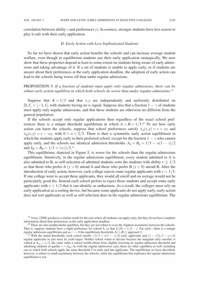
If the schools accept only regular applications then regardless of the exact school pref-erences there is a unique threshold equilibrium in which A = B = 1/3.20 To see how early action can harm the schools, suppose that school preferences satisfy πA(v, y) = v + αy and πB (v, y) = v −αy, with 0 < α < 2/3. There is then a symmetric early action equilibrium in which the students apply early to their preferred school, except for the fraction 1 −γ who cannot apply early, and the schools use identical admission thresholds: AE = BE = 1/3 −α(1 −γ)/2 and AR = BR = 1/3 + (αγ)/2.21
This equilibrium, depicted in Figure 5, is worse for the schools than the regular admissions equilibrium. Intuitively, in the regular admissions equilibrium, every student admitted to A is also admitted to B, so self-selection of admitted students sorts the students with ability v≥1/3 so that those who prefer A (y > 0) attend A and those who prefer B (y < 0) attend B. After the introduction of early action, however, each college rejects some regular applicants with v > 1/3. If one college were to accept these applicants, they would all enroll and on average would not be particularly good fits. Instead each school prefers to reject these students and accept some early applicants with v < 1/3 that it can identify as enthusiasts. As a result, the colleges must rely on early application as a sorting device, but because some applicants do not apply early, early action does not sort applicants as well as self-selection does in the regular admissions equilibrium. The
19 Avery (2008) produces a similar result for the case where all students can apply early, but they do not have complete information about their preferences at the early application deadline.
20 There are also nonthreshold equilibria, but they are not robust to even the slightest asymmetry between the schools. That is, suppose students have a slight preference for school A, so that gy(0) = 1/2 −ε. For each ε there is a unique regular admission equilibrium and as ε→0 the equilibrium thresholds A(ε), B(ε) approach V.
21 With the stated thresholds, each school enrolls γ[1/3 + α(1 −γ)/4] early applicants and (1 −γ)[1/3 −αγ/4] regular applicants to just meet its yield target. Neither school wants to deviate because the marginal early enrollee is valued at AEA + α/2, the same value a school would obtain from slightly lowering its regular admission threshold and admitting students of quality v = ARA. As with the regular admissions case, there are other equilibria as well, including one in which both schools apply the same threshold V to early and late applicants. The equilibrium we have described, however, is robust to small asymmetry between the schools, while the equilibrium that replicates the regular admissions equilibrium is not.
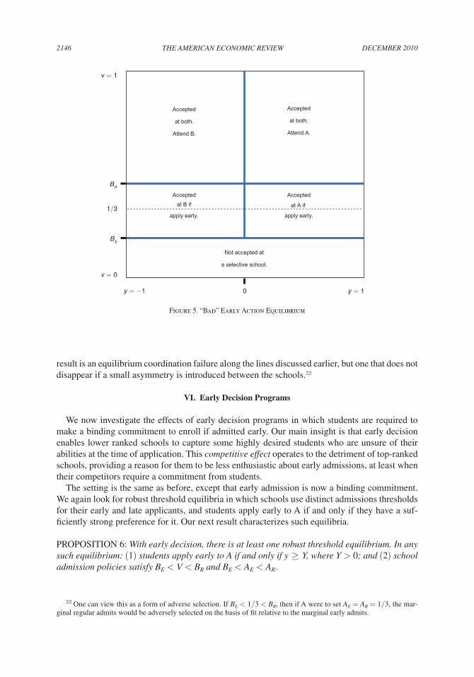
DEcEmBER 20102146 THE AmERIcAN EcONOmIc REVIEW
result is an equilibrium coordination failure along the lines discussed earlier, but one that does not disappear if a small asymmetry is introduced between the schools.22
VI. Early Decision Programs
We now investigate the effects of early decision programs in which students are required to make a binding commitment to enroll if admitted early. Our main insight is that early decision enables lower ranked schools to capture some highly desired students who are unsure of their abilities at the time of application. This competitive effect operates to the detriment of top-ranked schools, providing a reason for them to be less enthusiastic about early admissions, at least when their competitors require a commitment from students.
The setting is the same as before, except that early admission is now a binding commitment. We again look for robust threshold equilibria in which schools use distinct admissions thresholds for their early and late applicants, and students apply early to A if and only if they have a suf-ficiently strong preference for it. Our next result characterizes such equilibria.
PROPOSITION 6: With early decision, there is at least one robust threshold equilibrium. In any such equilibrium: (1) students apply early to A if and only if y≥Y, where Y > 0; and (2) school admission policies satisfy BE < V < BR and BE < AE < AR .
22 One can view this as a form of adverse selection. If BE < 1/3 < BR, then if A were to set AE = AR = 1/3, the mar-ginal regular admits would be adversely selected on the basis of fit relative to the marginal early admits.
Figure 5. “Bad” Early Action Equilibrium
Accepted
at both.
Attend A.
Not accepted at
a selective school.
Accepted
at both.
Attend B.
Acceptedat B if
apply early.
Accepted
at A if
apply early.
0
BE
BR
y = −1 y = 1
v = 1
1/3
v = 0
VOL. 100 NO. 5 2147AVERY AND LEVIN: EARLY ADmISSIONS AT SELEcTIVE cOLLEgES
The incentives with early decision are similar to the case of early action, although with a few differences. Consider the students. In equilibrium, students realize that there is an admissions benefit if they apply early to B, and students who prefer B take advantage of this. Students who prefer A have to trade off the admissions benefit of applying early to B against the cost of not being able to enroll at A if it turns out they have sufficient standing to be admitted. Applying early to B entails a benefit of u(B, y) if v is greater than min {AE, BR} and less than BE, and a loss of u(A, y)−u(B, y) if v≥AE. Therefore a student who prefers A will apply early to A if
(8) 1 − gv(AE|y)___
gv(min {AE, BR}|y) − gv(BE|y) u(A, y) − u(B, y)__
u(B, y) ≥ 1.
Both terms are increasing in y, and the left-hand side is equal to zero at y = 0. So the optimal policy for students involves a threshold Y > 0, just as with early action.
On the school side, A’s enrollees come entirely from its early applicant pool, because any stu-dent admitted regular has also been admitted to B and is obligated to enroll. So A’s early admis-sions threshold is pinned down by its enrollment target:
(9) m{v ≥ AE, y ≥ Y } = K.
School A is indifferent between a range of regular admissions thresholds, but we show in the Appendix that if the equilibrium is robust, A’s regular threshold must be set so that 피y[πA(v, y}|v = AR, y≥0 ] is just equal to the expected payoff from a marginal early admit, 피[πA(v, y)|v = AE, y≥Y ].
School B’s problem is similar to the early action case. In the equilibrium depicted earlier in Figure 3, school B must be just indifferent between a marginal enrollee from its early and regular applicant pools, so that (7) holds, and B must also admit just enough students to satisfy its yield target. The latter implies that in equilibrium
(10a) m {v ≥ BE, y < Y } + m {v ∈ [BR, AE ], y ≥ Y } = K.
As in the early action case, it is also possible to have an equilibrium in which school B fills its class entirely from its early applicant pool, in which case the optimality conditions are again similar to early action.
An interesting point about early decision equilibria is that the form of admission offered by school A is not important. All of the students who in equilibrium apply early to A would choose to attend even if the binding commitment was relaxed. So having A switch to a policy of early action would not affect the set of possible equilibria. Moreover, in equilibrium A fills its class entirely with students who chose not to apply early to B. So if A eliminates early admissions entirely, there is an equilibrium in which exactly the students who would have applied early to A instead submit only regular applications, and A applies its early decision threshold AE to all its applicants. This equilibrium gives rise to precisely the same allocation of students to schools.
This argument suggests why very top-ranked schools such as Harvard, Princeton, Yale, Stanford, and MIT may incur the least cost from moving away from early decision toward early action, or even from eliminating early admissions entirely. These schools have less reason to think they will lose top students by making the admissions commitment nonbinding. Flipping
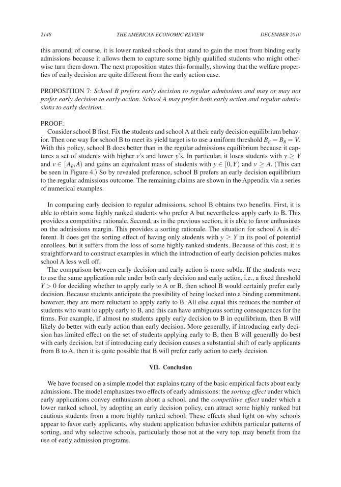
DEcEmBER 20102148 THE AmERIcAN EcONOmIc REVIEW
this around, of course, it is lower ranked schools that stand to gain the most from binding early admissions because it allows them to capture some highly qualified students who might other-wise turn them down. The next proposition states this formally, showing that the welfare proper-ties of early decision are quite different from the early action case.
PROPOSITION 7: School B prefers early decision to regular admissions and may or may not prefer early decision to early action. School A may prefer both early action and regular admis-sions to early decision.
PROOF: Consider school B first. Fix the students and school A at their early decision equilibrium behav-
ior. Then one way for school B to meet its yield target is to use a uniform threshold BE = BR = V. With this policy, school B does better than in the regular admissions equilibrium because it cap-tures a set of students with higher v’s and lower y’s. In particular, it loses students with y≥Y and v ∈[AE, A) and gains an equivalent mass of students with y ∈[0, Y ) and v≥A. (This can be seen in Figure 4.) So by revealed preference, school B prefers an early decision equilibrium to the regular admissions outcome. The remaining claims are shown in the Appendix via a series of numerical examples.
In comparing early decision to regular admissions, school B obtains two benefits. First, it is able to obtain some highly ranked students who prefer A but nevertheless apply early to B. This provides a competitive rationale. Second, as in the previous section, it is able to favor enthusiasts on the admissions margin. This provides a sorting rationale. The situation for school A is dif-ferent. It does get the sorting effect of having only students with y≥Y in its pool of potential enrollees, but it suffers from the loss of some highly ranked students. Because of this cost, it is straightforward to construct examples in which the introduction of early decision policies makes school A less well off.
The comparison between early decision and early action is more subtle. If the students were to use the same application rule under both early decision and early action, i.e., a fixed threshold Y > 0 for deciding whether to apply early to A or B, then school B would certainly prefer early decision. Because students anticipate the possibility of being locked into a binding commitment, however, they are more reluctant to apply early to B. All else equal this reduces the number of students who want to apply early to B, and this can have ambiguous sorting consequences for the firms. For example, if almost no students apply early decision to B in equilibrium, then B will likely do better with early action than early decision. More generally, if introducing early deci-sion has limited effect on the set of students applying early to B, then B will generally do best with early decision, but if introducing early decision causes a substantial shift of early applicants from B to A, then it is quite possible that B will prefer early action to early decision.
VII. Conclusion
We have focused on a simple model that explains many of the basic empirical facts about early admissions. The model emphasizes two effects of early admissions: the sorting effect under which early applications convey enthusiasm about a school, and the competitive effect under which a lower ranked school, by adopting an early decision policy, can attract some highly ranked but cautious students from a more highly ranked school. These effects shed light on why schools appear to favor early applicants, why student application behavior exhibits particular patterns of sorting, and why selective schools, particularly those not at the very top, may benefit from the use of early admission programs.

VOL. 100 NO. 5 2149AVERY AND LEVIN: EARLY ADmISSIONS AT SELEcTIVE cOLLEgES
The aspects of early admissions highlighted in our model are probably not the only reasons why schools have adopted such policies. One role of early admissions that we do not capture is yield management. Particularly at small colleges, there can be a significant downside to admitting too many students if it leads to crowded dorms or strained resources. At the same time, overly conserva-tive admissions decisions may require excessive reliance on the wait list. Admitting a fraction of the class early, with a binding commitment, can help to manage this risk.23 Schools may also want to increase yield for less benign reasons. Historically, yield was one of the metrics used by US News and World Report in its college rankings. This could have created an incentive for schools to rely more heavily on early decision in order to manipulate the rankings process.
For students, early decision policies also interact with the provision of financial aid. One issue of particular concern is that a binding early commitment may preclude a student from “shop-ping around” for the best financial aid package. This creates a dilemma for students with limited resources who want the admissions benefit of applying early.24 Of course, some students also may benefit from early admissions for reasons we have not emphasized. They may appreciate resolv-ing the anxiety of the application process earlier; receiving early notice of admission may allow them to avoid filling out additional applications.
It is also possible that for certain students the signaling effect of an early application is richer than in our specific model. For example, an early application from a high school that sends few students to selective colleges may indicate a promising level of ambition. Sam-Ho Lee (2009) has also highlighted a related informational issue, namely that if schools make noisy assessments of talent, early decision policies can protect a school against a winner’s curse in enrollment deci-sions. We observed a related phenomenon in the proof of Proposition 5, where we argued that under certain conditions schools might adopt early admission programs to match competitors but be collectively better off if these programs were eliminated.
Finally, we note that early admissions programs can be viewed as a form of “market unravel-ing” of the kind described by Alvin E. Roth and Xiaolin Xing (1994). In many of the markets they consider, a social cost of unraveling is that it appears to reduce the efficiency of market assignments by precluding the use of late-arriving information. Our analysis suggests that one benefit of early admissions may in fact be to increase the flow of information across the market by creating a cred-ible opportunity for students to signal interest. Nevertheless, a similar point can be made that by moving up the entire college admissions process, early admission programs force young students to make committing decisions even as their preferences may be evolving. Certainly all of these aspects of early application need to be considered if one is to evaluate possible reforms to the market.
Mathematical Appendix
Proof of Proposition 1
First, it is easy to see that if the schools use threshold policies, the yield constraints imply that m(v≥A, y≥0) = K (otherwise A would enroll either more or fewer than K students) and hence B = V. Now, consider any two admissions policies, not necessarily of threshold form. If B admits only students that are admitted by A, then B will enroll strictly fewer students than A. So satisfying both yield constraints implies there is some set of students [v′, v″] who are admitted only by B. In
23 Indeed, when Harvard and Princeton eliminated early admissions in 2007–08, both found that enrollment fell far short of target, leading to heavy reliance on their wait lists.
24 Kim (2010) argues that need-blind colleges could even use early decision programs to surreptitiously attract wealthy applicants. In practice, the latter concern seems somewhat unlikely given that the objectives of need-blind universities clearly go well beyond maximizing tuition revenue, and these institutions seem to be the ones that employ the least restrictive practices and are the most ambivalent about early admissions.
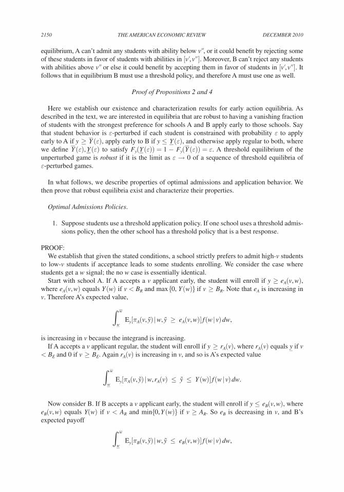
DEcEmBER 20102150 THE AmERIcAN EcONOmIc REVIEW
equilibrium, A can’t admit any students with ability below v″, or it could benefit by rejecting some of these students in favor of students with abilities in [v′, v″]. Moreover, B can’t reject any students with abilities above v″ or else it could benefit by accepting them in favor of students in [v′, v″]. It follows that in equilibrium B must use a threshold policy, and therefore A must use one as well.
Proof of Propositions 2 and 4
Here we establish our existence and characterization results for early action equilibria. As described in the text, we are interested in equilibria that are robust to having a vanishing fraction of students with the strongest preference for schools A and B apply early to those schools. Say that student behavior is ε-perturbed if each student is constrained with probability ε to apply early to A if y≥
_Y (ε), apply early to B if y ≤_Y (ε), and otherwise apply regular to both, where
we define _Y (ε), _ Y (ε) to satisfy Fy(_Y (ε)) = 1 −Fy(
_Y (ε)) = ε. A threshold equilibrium of the
unperturbed game is robust if it is the limit as ε→0 of a sequence of threshold equilibria of ε-perturbed games.
In what follows, we describe properties of optimal admissions and application behavior. We then prove that robust equilibria exist and characterize their properties.
Optimal Admissions Policies.
1. Suppose students use a threshold application policy. If one school uses a threshold admis-sions policy, then the other school has a threshold policy that is a best response.
PROOF: We establish that given the stated conditions, a school strictly prefers to admit high-v students
to low-v students if acceptance leads to some students enrolling. We consider the case where students get a w signal; the no w case is essentially identical.
Start with school A. If A accepts a v applicant early, the student will enroll if y≥eA(v, w), where eA(v, w) equals Y (w) if v < BR and max {0, Y (w)} if v≥BR. Note that eA is increasing in v. Therefore A’s expected value,
∫_w _w
Ey[πA(v, ̃ y )|w, ̃ y ≥ eA(v, w)]f (w|v)dw,
is increasing in v because the integrand is increasing.If A accepts a v applicant regular, the student will enroll if y≥rA(v), where rA(v) equals _y if v
< BE and 0 if v≥BE. Again rA(v) is increasing in v, and so is A’s expected value
∫ _ w _
w
E y[πA(v, ̃ y )|w, rA(v) ≤ ̃ y ≤ Y (w)]f (w|v)dw.
Now consider B. If B accepts a v applicant early, the student will enroll if y ≤eB(v, w), where eB(v, w) equals Y(w) if v < AR and min{0, Y (w)} if v≥AR. So eB is decreasing in v, and B’s expected payoff
∫ _ w _
w
Ey[πB(v, ̃ y )|w, ̃ y ≤ eB(v, w)]f (w|v)dw,
VOL. 100 NO. 5 2151AVERY AND LEVIN: EARLY ADmISSIONS AT SELEcTIVE cOLLEgES
is increasing in v, again because the integrand is increasing.Finally, if B accepts a v applicant regular, the student will enroll if v ≤rB(v), where rB(v)
equals _y if v < AE and 0 if v≥AE. So rB is decreasing in v, and B’s expected payoff
∫ _ w _
w
E y[πB(v, ̃ y )|w, Y (w) ≤ ̃ y ≤ rB(v)]f (w|v)dw,
is increasing in v.
2. Suppose students use a threshold application policy. Then each school has greater expected payoff from a v candidate who applied early than from a v candidate who applied regular.
PROOF: Consider school A. An early application reveals that y≥Y (w), so A’s average value from early
v applicants is at least Ew[πA(v, Y (̃ w ))|v ], and strictly higher provided Y (w) < _y for some frac-tion of w signals. Its value from regular v applicants is no greater than this amount. Similarly, B’s payoff from early (regular) v candidates is bounded below (above) by Ew[πB(v, Y (̃ w ))|v].
3. Suppose students use a threshold application policy. If one school uses a threshold policy, the other can optimally use a threshold policy that weakly favors early applicants.
PROOF: This follows from the previous two claims. If A considers a nonthreshold policy for one appli-
cant pool, switching to the highest threshold that satisfies the yield target will be at least a weak improvement. Similarly, if A considers thresholds AE > AR satisfying its yield target, lowering AE and raising AR while keeping yield constant will be at least a weak improvement. The same argument applies for school B.
4. Suppose students use a threshold application policy and school B uses a threshold admis-sion policy. Let α(Y, BE , BR) be A’s optimal threshold choices that satisfy AE ≤AR. Then α(Y, BE , BR) is nonempty, upper semicontinuous, convex, and compact-valued. The same properties hold for β(Y, AA, AR), similarly defined for school B.
PROOF: Consider school A. Given Y, BE, BR, it wants to choose thresholds AE ≤AR that meet its yield
target and achieve the highest expected payoff Ew, y[πA(v, ̃ y )|(v, ˜ w , ̃ y )∈], where denotes the set of types that will enroll and depends on its admission choices. The optimal policy (or policies) can be found constructively. Start with AE = AR equal to the unique value that satisfies the yield tar-get given Y, BE, BR.25 If there are no early applicants, this is the uniquely optimal choice of AR , and any AE is optimal. Similarly if there are no regular applicants, AE is uniquely optimal along with any AR. If there are early and late applicants but at the uniform thresholds no regular matriculants, i.e., if Y (w)≤0 for all w and AR≥BE, then AE is uniquely optimal along with any AR≥BE.
The last case is where the uniform threshold results in early and late matriculants. From the proof of Claim 2, the marginal early matriculant is strictly preferred to the marginal late matricu-lant. So consider lowering AE and raising AR while maintaining yield. By the proof of Claim 1,
25 Such a value always exists because a uniform threshold of _v results in no students, and dropping the threshold increases enrollment to an amount strictly greater than K at _v . We assume for convenience that the same is true for B (if B cannot always meet its yield target, a few small modifications are needed in the proof but our results still hold).
DEcEmBER 20102152 THE AmERIcAN EcONOmIc REVIEW
each such adjustment results in a strictly smaller improvement to average payoff. Continue until either: (i) the marginal matriculants are equal value, in which case we’ve found the unique opti-mum; or (ii) there are no regular matriculants (if AR hits BE and Y (w)≤0 for all w) in which case we’ve found the uniquely optimal AE, and any higher AR is optimal; or (iii) AE = _v in which case we’ve again found a unique optimum. In each case, optimal behavior involves AE < AR.
The constructive argument establishes that α(Y, BE, BR) is nonempty, compact, and convex. Upper semicontinuity follows from Berge’s Theorem (A’s average payoff objective is continuous in AE, AR, BE, BR, and Y, and its set of thresholds meeting the yield constraint is usc in Y, BE, BR).The same arguments apply for school B, showing that β(Y, AE, AR) has the stated properties and will want to strictly favor early applicants if a uniform admissions policy that meets the yield requirement leads to early and late matriculants.
5. Suppose student behavior is ε-perturbed. For sufficiently small ε, properties (1)–(4) above all hold. Furthermore α(Y, BE, BR; ε) and β(Y, AE, AR; ε) are upper semicontinuous in ε and for ε > 0, single-valued with strict preference for early applicants.
PROOF: The first three properties above follow from the same arguments. For small ε, each school
will still prefer to admit higher v students and prefer early to regular applicants. For the last part, consider the construction of optimal policies in the proof of Claim 4. For ε > 0, the uniform admissions policy leads to both early and late matriculants, so any optimal policy must involve strictly favoring early applicants, and in fact the optimal policy is unique. That α, β are usc in ε again follows from Berge’s Theorem.
Properties of Student Best Responses.
1. Suppose both schools strictly favor early applicants. If AE ≤BE, any student with y≥0 should apply early to A. If AE > BE, a student should apply early to A if y≥Y (w) and otherwise to B, where Y (w) is strictly positive and decreasing in w.
PROOF: If a student prefers a school and it has the lower early threshold, it’s optimal to apply early to that
school because for any realization of v applying early to the other school can only lead to worse outcomes. For the last claim, suppose AE > BE. It is optimal to apply early to A if and only if
(11) gv(AR|w, y) − gv(AE|w, y)___
gv(min {AE, BR}|w, y) − gv(BE|w, y) u(A, y) − u(B, y)__
u(B, y) ≥ 1.
The second term is strictly increasing in y and equal to zero at y = 0. The first term is strictly positive and weakly increasing in y by affiliation. So the student optimally uses a threshold rule: apply early to A if and only if y≥Y (w), where Y (w) > 0. Moreover, if w takes multiple values, the first term is increasing in w by affiliation, so Y (w) is decreasing.
2. Suppose the schools use thresholds that weakly favor early applicants. Then there is some threshold policy that is optimal for students with y≥0. Let γ(AE , AR , BE, BR) denote the set of threshold policies, nonincreasing in w, that are optimal for students subject to the constraint if y < 0 a student must apply early to B. Then γ is nonempty, convex-valued and usc in AE, AR, BE, BR.
VOL. 100 NO. 5 2153AVERY AND LEVIN: EARLY ADmISSIONS AT SELEcTIVE cOLLEgES
PROOF: If neither school strictly favors early applicants, any early application behavior is optimal
including all threshold rules, with Y (w)≥0 and nonincreasing in w. If only one school strictly favors early applicants, it is optimal to apply early to that school to the extent possible, again implying a threshold policy (either Y (w) = _y or Y (w) = 0 given the constraint). If both schools favor early applicants and AE ≤BE, then Y (w) = 0 is optimal given the constraint. Finally, if both favor early applicants and AE > BE, then there is a uniquely optimal threshold rule Y (w) > 0 as described above. From this characterization, it is straightforward to check that γ has the claimed properties.
Robust Threshold Equilibria.
1. Suppose student behavior is ε-perturbed, for sufficiently small ε > 0. At least one thresh-old equilibrium exists, and any threshold equilibrium involves BE < BR, BE < AE < AR, and either Y > 0 or if students have a signal of ability, Y (w) strictly positive and decreasing in w.
PROOF: Consider the case with a w signal. Let denote the set of possible admission thresholds AE, AR
with AE ≤AR, and similarly define . Let denote the set of application thresholds Y (w), with Y (w)≥0 and nonincreasing in w. Define the set-valued function:
T (Y, AE, AR, BE, BR; ε) = (α(Y, BE, BR; ε), β(Y, AE, AR; ε), γ(AE, AR, BE, BR)).
This correspondence maps ×× into itself. For sufficiently small ε > 0 satisfies all the requirements of the Glicksberg-Fan Fixed Point Theorem. Let Y (ε), AE (ε), AR(ε), BE (ε), BR(ε) denote a fixed point.
We claim these strategies are an equilibrium and satisfy the stated properties. By definition AE (ε), AR(ε) and BE(ε), BR(ε) are optimal for the schools, and from Claim 5 above, A and B must strictly favor early applicants. Moreover, we must have BE < AE. If instead AE ≤BE, any student with y > 0 that behaves optimally will enroll at A with at least probability 1 −ε when-ever v≥AE. So A’s yield constraint implies that AE > V, which in turn implies that less than 2K students are admitted to a selective school, violating optimality for the schools. Finally given that both A and B favor early applicants and BE < AE, it is strictly optimal for all students with y ≤0 to apply early to B. Therefore Y (ε) is the unique best-response for students even if we remove the constraints imposed in defining γ. Furthermore Y (w; ε) > 0.
2. There is always a robust threshold equilibrium of the unperturbed model, and any such equilibrium (a) students use a strictly positive threshold Y > 0, or if they have a w signal, a strictly positive and decreasing threshold Y (w); (b) schools thresholds satisfy BE < BR and BE < AE < AR; and (c) early yields exceed regular yields.
PROOF: Existence follows from the continuity properties established above. Consider a sequence of
strategies Y (ε), AE(ε), AR(ε), BE(ε), BR(ε) where for each ε > 0, the profile is an equilibrium. The sequence must have a convergent subsequence because ×× is compact. Moreover, if the limit Y, AE, AR, BE, BR were not an equilibrium some party could do strictly better with an alternative strategy. But that same strategy, say A′, will be preferred to AE, AR as a response to BE(ε), BR(ε), Y(ε) for sufficiently small ε, a contradiction.
DEcEmBER 20102154 THE AmERIcAN EcONOmIc REVIEW
We now establish necessary properties of a robust threshold equilibrium Y (w), AE, AR, BE, BR.First, AE ≤AR, BE ≤BR and Y (w)≥0, or else the equilibrium cannot be the limit of
ε-perturbed equilibria.Second, BE < AE. If instead AE ≤BE, then any student with y≥0 who behaves optimally will
enroll in A if v≥AE. So V < AE ≤BE, BR, AR, and hence less than 2K students are admitted in total to A and B violating the yield constraints.
Third, if A receives no early applications, i.e., Y (w) = _Y , its optimal policy must satisfy πA(AE, _
Y ) = Ey[πA(AR, y)|y≥0 ], and in particular AE < AR. This follows because A’s optimal policy must be the limit of optimal policies where A receives early applications from a vanishingly small fraction of students who prefer it most, and this limit must involve indifference (as opposed to AE = _v ) because AE > V.
Fourth, BE < BR. Suppose to the contrary that BE = BR. Because Y (w)≥0, B must receive early applicants, and some will enroll. If in addition B receives regular applications, some must sub-sequently enroll because BR = BE < AE. But that would mean a uniform threshold could not be optimal. So the only way that BE = BR could be optimal is if all students apply early to B. If that is so, however, then AE < AR from above, and we arrive at another contradiction to optimality because students with y > 0 would apply to A early if A but not B strictly favored early applicants.
Fifth, Y (w) > 0. This follows because B strictly favors early applicants and uses a strictly lower threshold than A for early applicants.
Sixth, AE < AR. We have already established this to be the case if A receives no early applica-tions, and if it receives early applications it must matriculate some of them. Moreover, because Y (w) > 0 it must matriculate some of its regular applicants if it uses a uniform threshold. So from (5) above, it must be the case that AE < AR.
The last property is that early yields exceed regular yields. This is clearly true for A, which enrolls all early admits. For B, it can be seen immediately in Figure 2, and the other cases are that either no students apply regular, which makes the claim trivial, or that BR > AE so that the regular yield is zero.
Proof of Proposition 6.
The argument is essentially the same as for propositions 2 and 4, so we provide only a sketch. First, it is easy to verify that optimal admissions and application behavior has the same proper-ties described above. Schools can optimally use threshold rules in response to threshold rules and want to strictly favor early applicants if they get matriculants from both pools. If the schools strictly favor early applicants and BE < AE, it is optimal for students to use a threshold policy with Y > 0. The existence of a robust threshold equilibrium follows from the same arguments made in the early action case.
Consider properties of a robust equilibrium. As above, we must have AE ≤AR, BE ≤BR and Y≥0. Similarly, we must have BE < AE to satisfy the yield constraints. It must also be the case that BE < BR. The only way this could not happen is if all students were applying early to B, in which case the yield constraints would imply that BE > AR≥AE violating the previous condi-tion. So BE < BR and BE < AE, and it follows that students must use a threshold Y > 0. Finally AE = AR is optimal for A but inconsistent with A’s thresholds being nearly optimal for small per-turbations in student application behavior along the lines above. So AE < AR.
Proof of Proposition 7.
The following example shows that preference toward early decision is sensitive to param-eters. Suppose v, y are independently distributed, with v uniform on [0, 1], and y taking values
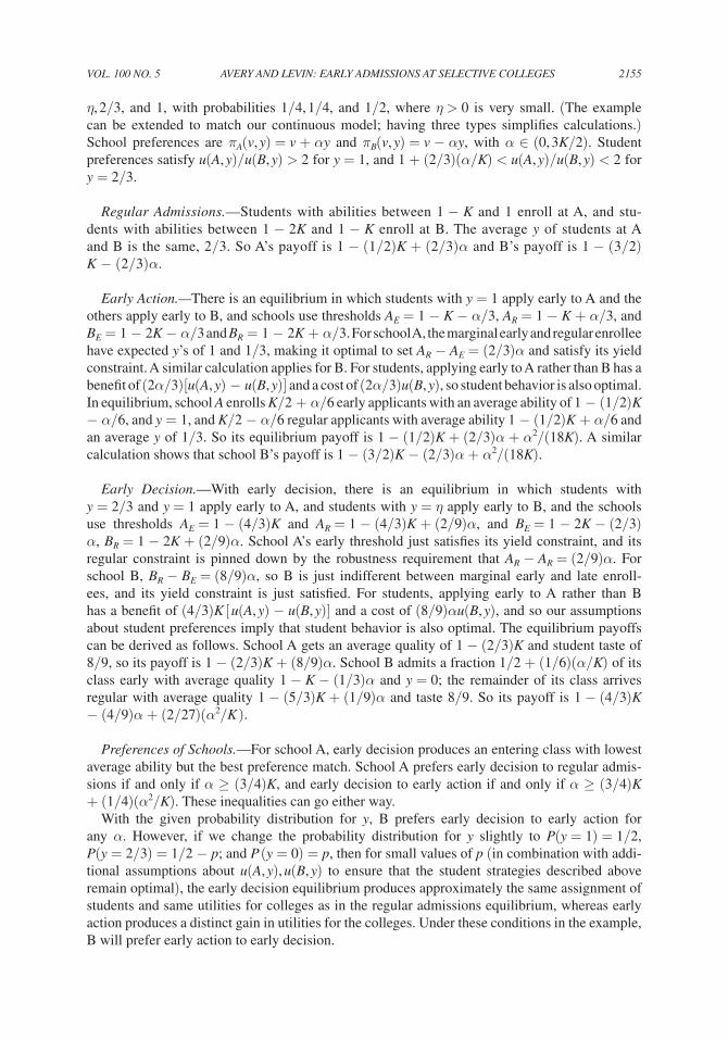
VOL. 100 NO. 5 2155AVERY AND LEVIN: EARLY ADmISSIONS AT SELEcTIVE cOLLEgES
η, 2/3, and 1, with probabilities 1/4, 1/4, and 1/2, where η > 0 is very small. (The example can be extended to match our continuous model; having three types simplifies calculations.) School preferences are πA(v, y) = v + αy and πB(v, y) = v − αy, with α∈(0, 3K/2). Student preferences satisfy u(A, y)/u(B, y) > 2 for y = 1, and 1 + (2/3)(α/K) < u(A, y)/u(B, y) < 2 for y = 2/3.
Regular Admissions.—Students with abilities between 1 − K and 1 enroll at A, and stu-dents with abilities between 1 − 2K and 1 − K enroll at B. The average y of students at A and B is the same, 2/3. So A’s payoff is 1 − (1/2)K + (2/3)α and B’s payoff is 1 − (3/2)K − (2/3)α.
Early Action.—There is an equilibrium in which students with y = 1 apply early to A and the others apply early to B, and schools use thresholds AE = 1 − K − α/3, AR = 1 − K + α/3, and BE = 1 − 2K − α/3 and BR = 1 − 2K + α/3. For school A, the marginal early and regular enrollee have expected y’s of 1 and 1/3, making it optimal to set AR − AE = (2/3)α and satisfy its yield constraint. A similar calculation applies for B. For students, applying early to A rather than B has a benefit of (2α/3)[u(A, y) − u(B, y)] and a cost of (2α/3)u(B, y), so student behavior is also optimal. In equilibrium, school A enrolls K/2 + α/6 early applicants with an average ability of 1 − (1/2)K− α/6, and y = 1, and K/2 − α/6 regular applicants with average ability 1 − (1/2)K + α/6 and an average y of 1/3. So its equilibrium payoff is 1 − (1/2)K + (2/3)α + α2/(18K). A similar calculation shows that school B’s payoff is 1 − (3/2)K − (2/3)α + α2/(18K).
Early Decision.—With early decision, there is an equilibrium in which students with y = 2/3 and y = 1 apply early to A, and students with y = η apply early to B, and the schools use thresholds AE = 1 − (4/3)K and AR = 1 − (4/3)K + (2/9)α, and BE = 1 − 2K − (2/3)α, BR = 1 − 2K + (2/9)α. School A’s early threshold just satisfies its yield constraint, and its regular constraint is pinned down by the robustness requirement that AR − AR = (2/9)α. For school B, BR − BE = (8/9)α, so B is just indifferent between marginal early and late enroll-ees, and its yield constraint is just satisfied. For students, applying early to A rather than B has a benefit of (4/3)K [u(A, y) − u(B, y)] and a cost of (8/9)αu(B, y), and so our assumptions about student preferences imply that student behavior is also optimal. The equilibrium payoffs can be derived as follows. School A gets an average quality of 1 − (2/3)K and student taste of 8/9, so its payoff is 1 − (2/3)K + (8/9)α. School B admits a fraction 1/2 + (1/6)(α/K) of its class early with average quality 1 − K − (1/3)α and y = 0; the remainder of its class arrives regular with average quality 1 − (5/3)K + (1/9)α and taste 8/9. So its payoff is 1 − (4/3)K − (4/9)α + (2/27)(α2/K ).
Preferences of Schools.—For school A, early decision produces an entering class with lowest average ability but the best preference match. School A prefers early decision to regular admis-sions if and only if α≥(3/4)K, and early decision to early action if and only if α≥(3/4)K + (1/4)(α2/K). These inequalities can go either way.
With the given probability distribution for y, B prefers early decision to early action for any α. However, if we change the probability distribution for y slightly to P(y = 1) = 1/2, P(y = 2/3) = 1/2 − p; and P (y = 0) = p, then for small values of p (in combination with addi-tional assumptions about u(A, y), u(B, y) to ensure that the student strategies described above remain optimal), the early decision equilibrium produces approximately the same assignment of students and same utilities for colleges as in the regular admissions equilibrium, whereas early action produces a distinct gain in utilities for the colleges. Under these conditions in the example, B will prefer early action to early decision.
DEcEmBER 20102156 THE AmERIcAN EcONOmIc REVIEW
REFERENCES
Avery, Christopher. 2008. “Preferences and Signaling in Matching Markets.” Unpublished.Avery, Christopher, Andrew Fairbanks, and Richard Zeckhauser. 2002. “What Worms for the Early Bird:
Early Admissions at Elite Colleges.” Unpublished.Avery, Christopher, Andrew Fairbanks, and Richard Zeckhauser. 2003. The Early Admissions game: Join-
ing the Elite. Cambridge, MA: Harvard University Press.Chade, Hector, Greg Lewis, and Lones Smith. 2010. “A Supply and Demand Model of the College Admis-
sions Problem.” http://tippie.uiowa.edu/economics/tow/papers/chade_spring2009.pdf.Hoxby, Caroline M. 2009. “College Admissions: The Changing Selectivity of American Colleges.” Journal
of Economic Perspectives, 23(4): 95–118.Kim, Matthew. 2010. “Early Decision and Financial Aid Competition among Need-Blind Colleges and Uni-
versities.” Journal of Public Economics, 94(5–6): 410–20.Lee, Sam-Ho. 2009. “Jumping the Curse: Early Contracting with Private Information in University Admis-
sions.” International Economic Review, 50(1): 1–38.Lien, Yuan-Chuan. 2009. “Application Choices and College Rankings.” http://www.ylien.com/
AppChoice20090425.pdfRamey, Garey, and Valerie A. Ramey. 2010. “The Rug-Rat Race.” http://www.econ.ucsd.edu/~vramey/
research/Rugrat.pdf.Roth, Alvin E., and Xiaolin Xing. 1994. “Jumping the Gun: Imperfections and Institutions Related to the
Timing of Market Transactions.” American Economic Review, 84(4): 992–1044.