Efficient Perturbation Methods for SolvingSwitching DSGE Models

Junior Maih∗

Norges Bankjunior.maih@norges-bank.no

December 15, 2014

Abstract

In this paper we present a framework for solving switching nonlinear DSGEmodels. In our approach, the probability of switching can be endogenous andagents may react to anticipated events. The solution algorithms derived aresuitable for solving large systems. They use a perturbation strategy which,unlike Foerster et al. (2014), does not rely on the partitioning of the switchingparameters and is therefore more efficient. The algorithms presented are allimplemented in RISE, an object-oriented toolbox that is flexible and can easilyintegrate alternative solution methods. We apply our algorithms to and canreplicate various examples found in the literature. Among those examples is aswitching RBC model for which we present a third-order perturbation solution.

JEL C6, E3, G1.

∗First version: August 1, 2011. The views expressed herein are mine and do not necessarilyrepresent those of Norges Bank. Some of the ideas in this paper have often been presented underthe title : ”Rationality in Switching Environments”. I would like to thank Dan Waggoner, Tao Zha,Hilde Bjørnland, and seminar participants at the Atlanta Fed (Sept. 2011), IMF, Norges Bank,JRC, the National Bank of Belgium, dynare conferences (Zurich, Shanghai), Venastul, Board ofGovernors of the Federal Reserve System and the 87th WEAI conference in San Francisco.

1

1 Introduction

In an environment in where economic structures break, variances change, distribu-tions shift, conventional policies weaken and past events (e.g. crises) tend to reoc-cur, the Markov switching DSGE (MSDSGE) model appears as the natural frame-work for analyzing the dynamics of macroeconomic variables12. MSDSGE modelsare also important because many policy questions of interest seem to be best an-swered/addressed in a framework of changing parameters3.

Not surprisingly then, besides the ever-growing empirical literature using MS-DSGE models, many efforts have been invested in solving those models. In thatrespect, the literature has considered 3 main angles of attack. One strand of litera-ture considers approximating the solution of those models using ”global” methods.Examples include Davig et al. (2011), Bi and Traum (2013) and Richter et al. (2014).Just like in constant-parameter models, global approximation methods in switching-parameter models face problems of curse of dimensionality, reliance on a pre-specifiedset of grid points typically constructed around one steady state although the modelmay have many, etc. The curse of dimensionality in particular, implies that the num-ber of state variables has to be as small as possible and even solving small modelsinvolves substantial computational costs.

A second group of techniques applies Markov switching to the parameters oflinear or linearized DSGE models. Papers in this class include Farmer et al. (2011),Cho (2014), Svensson and Williams (2007) to name a few. One advantage of thisapproach is that one can handle substantially larger problems than the ones solvedusing global methods. Insofar as the starting point is a linear model, all one has to

1Changes in shock variances have been documented by Stock and Watson (2003), Sims and Zha(2006), Justiniano and Primiceri (2008), while breaks in structural parameters have been advocatedby Bernanke et al. (1999), Lubik and Schorfheide (2004), Davig and Leeper (2007). Other papershave also documented changes in both variances and structural parameters. Examples include Smetsand Wouters (2007), Svensson and Williams (2007, Svensson and Williams (2009) and Cogley et al.(2012).

2In such a context, constant-parameter models could be misleading in their predictions and theirimplications for policymaking.

3Some of those questions are:

• what actions should we undertake today given the non-zero likelihood of a bad state occurringin the future?

• What can we expect of the dynamics of the macro-variables we care about when policy isconstrained?

• How is the economy stabilized when policy is constrained?

2

worry about is how to compute and characterize the solution of the model. If theoriginal model is nonlinear, however, a first-order approximation may not be sufficientto approximate the nonlinear dynamics implied by the true policy functions of themodel. The nonlinearity of the original model also implies that one cannot assumeaway the switches in the parameters for the sake of linearization and then re-applythem to the model parameters once the linearized form is obtained. Consistentlylinearizing the model while taking into account the switching parameters calls for adifferent strategy.

Finally, the third group of techniques attempts to circumvent or find a work-around to the problems posed by the first two groups. More specifically, this liter-ature embeds switching in perturbation solutions whose accuracy can be improvedwith higher and higher orders4. This is the approach followed by Foerster et al.(2014) and in this paper.

For many years, we have been developing, in the RISE toolbox, algorithms forsolving and estimating models of switching parameters including DSGEs, VARs,SVARs, optimal policy models of commitment, discretion and loose commitment5.In the present paper, however, we focus on describing the theory behind the routinesimplementing the switching-parameter DSGE in RISE6.

Our approach is more general than the ones discussed earlier or found in theliterature. In contrast to Foerster et al. (2014) and the papers cited above, in ourderivation of higher-order perturbations we allow for endogenous transition proba-bilities. We also allow for anticipated events following Maih (2010) and Juillard andMaih (2010). This feature is useful as it offers an alternative to the news shocks

4Model accuracy is often measured by the Euler approximation errors. It is important to notethat a high accuracy is not synonymous with the computed policy functions being close to the trueones

5RISE is a matlab-based object-oriented toolbox. The flexibility and modularity of the toolboxare such that any user with little exposure to RISE is able to apply his own solution methodwithout having to change anything to the core codes. The toolbox is available, free of charge, athttps://github.com/jmaih/RISE toolbox.

6We plan to describe algorithms for other modules of RISE in subsequent papers.

3

strategy that has often been used to analyze the effects of forward guidance78. Theintroduction of an arbitrary number of anticipated shocks does come at a cost though:the number of cross terms to keep track of increases rapidly with the order of ap-proximation and computing those terms beyond the first order becomes intractable.This problem is circumvented by exploiting a simple trick by Levintal (2014), whoshows a way of computing higher-order approximations by keeping all state variablesin a single block9.

But before computing higher-order perturbations, two problems relative to thechoice of the approximation point and the solving of a quadratic matrix equation,have to be addressed. With respect to the choice of the approximation point, Foer-ster et al. (2014) propose a ”partition perturbation” strategy in which the switchingparameters are separated into two groups: one group comprises the switching pa-rameters that affect the (unique) steady state and another group that collects theswitching parameters that do not affect the steady state. Here also, the approachimplemented in RISE is more general, more flexible and simpler: it does not requireany partitioning of the switching parameters and is therefore more efficient. More-over, it allows for the possibility of multiple steady states and delivers the results of

7There are substantial differences between what this paper calls ”anticipated events” or ”an-ticipated shocks” and ”news shocks”. First, solving the model with anticipated shocks does notrequire a modification of the equations of the original system, in contrast to ”news shocks” thatare typically implemented by augmenting the law of motion of a shock process with additionalshocks. Secondly, in the anticipated shocks approach, future events are discounted while in thenews shocks approach the impact of a news shock does not depend on the horizon at which thenews occurs. Thirdly, an anticipated shock is genuinely a particular structural shock in the originalsystem, while in the news shocks, it is a different iid shock with no other interpretation than ”anews” and unrelated to any structural shock in the system. Because it is unrelated, it will have itsown distribution independently of other parts of the system. Fourthly, the estimation of modelsof news shocks requires additional variables to be declared as observables and enter the measure-ment equation. The estimation procedure tries to fit the future information is the same way it fitsthe other observable variables. This feature makes Bayesian model comparison infeasible since thecomparison of two models requires that they have the same observable variables. In contrast, in theestimation of models with anticipated shocks, the anticipated information, which may not materi-alize is separated from the actual data. Model comparison remains possible since the anticipatedinformation never enters the measurement equations. Finally, in the anticipated shocks approachthe policy functions are explicitly expressed in terms of leads of future shocks as opposed to lags inthe news shocks approach.

8In particular, it makes it possible to analyze the effects of hard conditions as well as soft con-ditions on the future information The discounting of future events also depends on the uncertaintyaround those events.

9Before the new implementation, the higher-order perturbation routines of RISE separated thestate variables into three blocks: endogenous variables, perturbation parameter, exogenous shocks.Cross products of those had to be taken explicitly, calculated and stored separately.

4

the ”partition perturbation” of Foerster et al. (2014) as a special case.When it comes to solving the system of quadratic matrix equations implied by

the first-order perturbation, Foerster et al. (2014)’s proposal is to use the theory ofof Grobner bases (see Buchberger (1965, Buchberger (2006)) to find all the solutionsof the system and then apply the engineering concept of mean square stability toeach of the solutions as a way to check whether the Markov switching system admitsa single stable solution. While recognizing the benefits of a procedure that can gen-erate all possible solutions of a nonlinear system and even plan to integrate a similarprocedure in RISE, we argue that such an approach may not be practical or suit-able for systems of the size that we have been accustomed to in constant-parameterDSGE models10. Furthermore the approach also has two major limitations: (1)stability of first-order approximation does not imply stability of higher-order ap-proximations, even in constant-parameter DSGE models; (2) there is no stabilityconcept for switching models with endogenous transition probabilities.

Because we are ultimately interested in estimating those models in order to makethem really useful for policymaking, we take a more modest route: we derive efficientfunctional iterations and Newton algorithms that are suitable for solving relativelylarge systems. As an example, we have successfully solved a second-order pertur-bation of a model of 272 equations using our algorithms. We further demonstratethe efficiency and usefulness of our solution methods by applying them to variousexamples found in the literature. Our algorithms easily replicate the results foundby other authors. Among the examples we consider is a switching model by Foersteret al. (2014) for which we present a third-order perturbation solution.

The rest of the paper proceeds as follows. Section 2 introduces the notationwe use alongside the generic switching model that we aim to solve. Then section3 derives the higher-order approximations of the model. At the zero-th order, wepresent various flexible strategies for choosing the approximation point. Section 4takes on the solving of the quadratic matrix polynomial arising in the first-orderapproximation. Section 5 evaluates the performance of the proposed algorithms andsection 6 concludes.

10Grobner bases have problems of their own and we will return to some of them later in the text.

5

2 The Markov Switching Rational Expectations

Model

2.1 The economic environment

We are interested in characterizing an environment in which parameters switch ina model that is potentially already nonlinear even in the absence of switching pa-rameters. In that environment we would like to allow for the transitions controllingparameter switches to be endogenous and not just exogenous as customarily found inthe literature. Finally, recognizing that at the time of making decisions agents mayhave information about future events, it is desirable that in our framework futureevents –forward guidance on the behavior of policy is an example of such a possibility– ,which may or many not materialize in the end, influence the current behavior ofprivate agents.

2.2 Dating and notation conventions

The dating convention used in this paper is different from the widely used conventionof Schmitt-Grohe and Uribe (2004) in which the dating of the variables refers to thebeginning of the period. Instead we use the also widely used dating convention inwhich the dating of the variables refers to the end of the period. In that way, thedating determines the period in which the variable of interest is known. This is thetype of notation used for instance in Adjemian et al. (2011).

Some solution methods for constant-parameter DSGE models (e.g. Klein (2000),Gensys, Schmitt-Grohe and Uribe (2004)) stack variables of different periods. Thistype of notation has also been used in switching-parameter DSGE models by Farmeret al. (2011), Foerster et al. (2013). This notation is not appropriate for the typeof problems this paper aims to solve. In addition to forcing the creation of auxiliaryvariables and thereby increasing the size of the system, it also makes it cumbersome tocompute expectations of variables in our context since future variables could belongto a state that is different from the current one. Clearly, doing so may restrict theclass of problems one can solve or give the wrong answer in some types of problems11. The stacking of different time periods therefore is not appealing for our purposes.

11In the Farmer et al. (2011) procedure for instance, the Newton algorithm is constructed on theassumption that the coefficient matrix on forward-looking variables depends only on the currentregime.

6

2.3 The generic model

Many solution approaches, like Farmer et al. (2011) or Cho (2014), start out with alinear model and then apply a Markov switching to the parameters. This strategy isreasonable as long as one takes a linear specification as the structural model. Whenthe underlying structural model is nonlinear, however, the agents are aware of thenonlinear nature of the system and the switching process. This has implications forthe solutions based on approximation and for the decision rules. In this setting, animportant result by Foerster et al. (2013) is that the first-order perturbation maybe non-certainty equivalent. Hence starting out with a linear specification may missthis important point.

The problem to solve is

Et

h∑rt+1=1

πrt,rt+1 (It) drt (v) = 0

where Et is the expectation operator, drt : Rnv −→ Rnd is a nd× 1 vector of possiblynonlinear functions of their argument v (defined below), rt = 1, 2, .., h is the regimea time t, πrt,rt+1 (It) is the transition probability for going from regime rt in thecurrent period to regime rt+1 in the next period. This probability is potentiallyendogenous in the sense that it is a function of It, the information set at time t.The only restriction imposed on the endogenous switching probabilities is that theparameters affecting them do not switch over time and that the variables enteringthose probabilities have a unique steady state12.

The nv × 1 vector v is defined as

v ≡[bt+1 (rt+1)′ ft+1 (rt+1)′ st (rt)

′ pt (rt)′ bt (rt)

′ ft (rt)′ p′t−1 b′t−1 ε′t θ′rt+1

]′(1)

where st is a ns×1 vector of static variables13, ft is a nf×1 vector of forward-lookingvariables14, pt is a np × 1 vector of predetermined variables15, bt is a nb × 1 vectorof variables that are both predetermined and forward-looking, εt is a nε × 1 vectorof shocks with εt ∼ N (0, Inε) and θrt+1 is a nθ × 1 vector of switching parameters(appearing with a lead in the model).

Note that we do not declare the parameters of the current regime rt. They areimplicitly attached to drt . Also note that we could get rid of the parameters of future

12RISE automatically checks for these requirements13Those are the variables appearing in the model only at time t.14Those variables appearing in the model both time t and in future periods t+ 1, t+ 2, etc..15Those variables appear in the model at time t and at times t− 1, t− 2, etc.

7

regimes (θrt+1) by declaring auxiliary variables, which would then be forward-lookingvariables.

If we define the nd × 1 vector drt,rt+1 as drt,rt+1 ≡ πrt,rt+1 (It) drt , the objectivebecomes

Et

h∑rt+1=1

drt,rt+1 (v) = 0 (2)

We assume that the agents have information for all or some of the shocks k ≥ 0periods ahead into the future. And so, including a perturbation parameter σ, wedefine an nz × 1 vector of state variables as

zt ≡[p′t−1 b′t−1 σ ε′t ε′t+1 · · · ε′t+k

]′where nz = np + nb + (k + 1)nε + 1.

Denoting by yt (rt), the ny × 1 vector of all the endogenous variables, whereny = ns + np + nb + nf , we are interested in solutions of the form

yt (rt) ≡

st (rt)pt (rt)bt (rt)ft (rt)

= T rt (zt) ≡

Srt (zt)Prt (zt)Brt (zt)F rt (zt)

(3)

In general, there is no analytical solution to (2) even in cases where drt or drt,rt+1

is linear. In this paper we rely on a perturbation that will allow us to approximatethe decision rules in (3)16. We can then solve these approximated decision rules byinserting their functional forms into (2) and its derivatives. This paper developsmethods for doing that.

For the subsequent derivations, it is useful to define for all g ∈ s, p, b, f, anng × ny matrix λg that select the solution of g-type variables in T or y. We also

define λx ≡[λpλb

]and λbf ≡

[λbλf

]as the selector for p-b and b-f variables

respectively. In the same way, we define for all g ∈ pt−1, bt−1, σ, εt, εt+1, ..., εt+k, amatrix mg of size ng × nz that selects the g-type variables in the state vector zt.

16Alternatively one could approximate (2) directly as it is done for instance in Dynare.

8

3 Approximations

Since the solution is in terms of the vector of state variables zt, we proceed toexpressing all the variables in the system as a function of zt

17. Since both bt+1 (rt+1)and ft+1 (rt+1) appear in the system (1) and given the solution (3) we need to expresszt+1 as a function of zt. This is given by

zt+1 = hrt (zt) + uzt

where

hrt (zt) ≡[

(λxT rt (zt))′ (mσzt)

′ (mε,1zt)′ · · · (mε,kzt)

′ (0nε×1)′]′

and u is a nz × nz random matrix defined by

u ≡[

0(np+nb+1+knε)×nzεt+k+1mσ

](4)

Following Foerster et al. (2014) , we postulate a perturbation solution for θrt+1

as18

θrt+1 = θrt + σθrt+1 (5)

In this respect, this paper differs from Foerster et al. (2013) and Foerster et al.(2014) in two important ways. First, θrt need not be the ergodic mean of the pa-rameters as will be discussed below. Secondly, conditional on being in regime rtperturbation is never done with respect to the θrt parameters. Perturbation is doneonly with respect to the parameters of the future regimes (θrt+1) that appear in thesystem for the current regime (rt).

Given the solution, we can now express vector v in terms of the state variables

v =

λbfT rt+1 (hrt (zt) + uzt)T rt (zt)mpztmbztmε,0zt

θrt + θrt+1mσzt

(6)

17Here we differentiate the policy functions. One could, alternatively, differentiate the modelconditions as done for instance in Dynare and Dynare++. This would involve taking the Taylorexpansion of the original objective (2).

18This assumption is not necessary. We could, as argued above, simply declare new auxiliaryvariables and get rid of the parameters of the future regimes.

9

and the objective function (2) becomes

Et

h∑rt+1=1

drt,rt+1 (v (zt, εt+k+1)) = 0 (7)

Having expressed the problem to solve in terms of state variables in a consol-idated vector zt, as in Levintal (2014), we stand ready to take successive Taylorapproximations of 7 to find the perturbation solutions.

3.1 Zero-th order

The first step of the perturbation technique requires the choice of the approximationpoint. In a constant-parameter world, we typically approximate the system aroundthe steady state, the resting point to which the system will converge in the absenceof future shocks. In a switching environment the choice is not so obvious any more.

Approximation around the ergodic mean Foerster et al. (2014) propose totake a perturbation of the system around its ergodic mean. This ergodic mean canbe found by solving

drt(bt, ft, st, pt, bt, ft, pt, bt, 0, θ

)= 0

where θ is the ergodic mean of the parameters19. The ergodic mean is, however,need not be an attractor or a resting point, a point towards which the system willconverge in the absence of further shocks. We propose two further possibilities.

Regime-specific steady states20 The first one is to approximate the systemaround regime-specific means. The system may not be stable at the mean in acertain regime, but at least we assume that if the system happens to be exactlyat one of its regime-specific means, it will stay there in the absence of any furthershocks. We compute those means by solving

drt (bt (rt) , ft (rt) , st (rt) , pt (rt) , bt (rt) , ft (rt) , pt (rt) , bt (rt) , 0, θrt) = 0

The intuition behind this strategy is two-fold. On the one hand, it is not toodifficult to imagine that the relevant issue for rational agents living in a particular

19In the RISE toolbox, this is triggered by the option ”unique”.20This approach is the default behavior in the RISE toolbox.

10

state of the system at some point in time, is to insure against the possibility ofswitching to a different state, and not to the ergodic mean. On the other hand, froma practical point of view, the point to which the system is to return matters forforecasting. Many inflation-targeting countries, have moved from a regime of highinflation to a regime of lower inflation. Approximating the system around the ergodicmean in this case implies that the unconditional forecasts will be pulled towards alevel that is consistently higher than the recent history of inflation, which is likelyto yield substantial forecast errors. All this contributes to reinforcing the idea thatthe ergodic mean is not necessarily an attractor.

Approximation around an arbitrary point In the second possibility, one canimpose an arbitrary approximation point. If the chosen point of approximationis chosen arbitrarily, obviously, none of the two equations above will hold and acorrection will be needed in the dynamic system, with consequences for the solutionas well. This approach may be particularly useful in certain applications, e.g. asituation in which one of the regimes persistently deviates from the reference steadystate for an extended period of time21. The approach also bears some similarity withthe constant-parameter case where the approximation is sometimes taken around therisky or stochastic steady state.

Suppose we want to take an approximation around an arbitrary point[s, p, b, f

].

The strategy we suggest is to evaluate that point in each regime. More specificallywe will have

drt ≡ drt

(b, f , s, p, b, f , p, b, 0, θrt , θrt

)This discrepancy is then forwarded to the first-order approximation when solving

the first-order coefficients.Interestingly, both the regime-specific approach and the ergodic approach are spe-

cial cases. In the former, because[s, p, b, f

]= [st (rt) , pt (rt) , bt (rt) , ft (rt)], the dis-

crepancy, drt , is zero. In the later case,[s, p, b, f

]=[sergodic, pergodic, bergodic, f ergodic

]and the discrepancy need not be zero.

The approach suggested here is computationally more efficient than that sug-gested by Foerster et al. (2014) and does not require any partitioning of the switch-ing parameters between those that affect the steady state and those that do not. Itwill be shown later on in an application that we recover their results.

21In the RISE toolbox, this is triggered by the option ”imposed”. When the steady state is notimposed, RISE uses the values provided as an initial guess in the solving of the approximation point

11

3.2 First-order perturbation

Taking high-order approximations of this system is tedious especially if one attemptsto compute all cross/partial derivatives in isolation. This is even worse if one allowsfor anticipated events. A less cumbersome approach exploits the strategy of Levintal(2014) in which the differentiation is done with respect to the entire vector z directly,rather than element by element or block by block22. At first order, then, we seek toapproximate T rt in (3) with a solution of the form

T rt (z) ' T rt (zrt) + T rtz (zt − zrt) (8)

Finding this solution requires differentiating (7) with respect to zt and applyingthe correction due to the choice of the approximation point, which is equivalent totaking a first-order Taylor expansion of (7). Using tensor notation, we have

[drt

]i+ Et

h∑rt+1=1

[drt,rt+1v ]iα [vz]

αj = 0 (9)

where [drt,rt+1v ]iα denotes the derivative of the ith row of d with respect to the αth row

of v and, similarly, [vz]αj denotes the derivative of the αth row of v with respect to

the jth row of z.Defining

A0rt,rt+1

≡[drt,rt+1

s0 drt,rt+1

p0 drt,rt+1

b0 drt,rt+1

f0

]we have

dv =[drt,rt+1

b+ drt,rt+1

f+ A0rt,rt+1

drt,rt+1

p− drt,rt+1

b− drt,rt+1

ε0 drt,rt+1

θ+

]The equality in (9) follows from the fact that all the derivatives of (7) must be

equal to 0. The derivatives of v with respect to z are given by

vz = a0z + a1

zu (10)

where the definitions of a0z and a1

z are given in appendix (A.1).The derivative of h with respect to z need in the calculation of vz, as can be seen

in (6), is given by

hrtz =[

(λxT rtz )′ m′σ m′ε,1 · · · m′ε,k 0n2z×nε

]′22This strategy is particularly useful when it comes to computing higher-order cross derivatives.

By not separating state variables, we always one block of cross products no matter the order ofapproximation instead of an exponentially increasing number of cross blocks.

12

Unfolding the tensors this problem reduces to

drt +h∑

rt+1=1

drt,rt+1v Etvz = 0

Let’s define drt,rt+1

gq ≡ ∂drt,rt+1

∂gqfor g = s, p, f, b referring to static, predetermined, for-

ward looking and ”both” variables and for q = 0,+,− referring to current variables,future variables and past variables respectively. The problem can be expanded into

h∑rt+1=1

[drt,rt+1

b+ drt,rt+1

f+

]λbfT rt+1

z hrtz + A0rt,rt+1

T rtz +[drt,rt+1

p− drt,rt+1

b−

] [ mp

mb

]+ d

rt,rt+1

ε0 mε,0 + drt,rt+1

θ+ θrt+1mσ

= 0

Looking at T rtz and hrtz in detail, we see that they can be partitioned. In particular,with

T rtz,x ≡[T rtz,p T rtz,b

]we have

T rtz =[T rtz,x T rtz,σ T rtz,ε0 T

rtz,ε1 · · · T

rtz,εk

]

hrtz =

λxT rtz,x λxT rtz,σ λxT rtz,ε0 λxT rtz,ε1 · · · λxT rtz,εk01×nx 1 01×nε 01×nε · · · 01×nε0nε×nx 0nε×1 0nε Inε · · · 0nε

......

......

. . ....

0nε×nx 0nε×1 0nε 0nε · · · Inε0nε×nx 0nε×1 0nε 0nε · · · 0nε

Hence the solving can be decomposed into small problems

3.2.1 Impact of endogenous state variables

The problem to solve is

0 = A0rtT

rtz,x + A−rt +

∑hrt+1=1A

+rt,rt+1

T rt+1z,x λxT rtz,x (11)

with

A0rt ≡

h∑rt+1=1

A0rt,rt+1

13

A−rt ≡h∑

rt+1=1

[drt,rt+1

p− drt,rt+1

b−

]A+rt,rt+1

≡[

0nd×ns 0nd×np drt,rt+1

b+ drt,rt+1

f+

](12)

Since there are many algorithms for solving (11), we delay the presentation ofour solution algorithms until section 4. For the time being, the reader should notethe way A+

rt,rt+1enters (11). This says that our algorithms will be able to handle

cases where the coefficient matrix on forward-looking terms is known in the currentperiod (A+

rt,rt+1= A+

rt,rt) as in Farmer et al. (2011) but also the more complicatedcase where A+

rt,rt+16= A+

rt,rt as in Cho (2014). This is part of the reasons why thenotation of Schmitt-Grohe and Uribe (2004), where one can stack variables is notappropriate in this context. This assumption is very convenient in the Farmer et al.(2011) algorithm as it allows them to derive their solution algorithm, which would bemore difficult otherwise. It is also convenient as it leads to substantial computationalsavings. But as our the derivations show, the assumption is incorrect in problemswhere A+

rt,rt+16= A+

rt,rt .

3.2.2 Impact of uncertainty

For the moment, we proceed with the assumption that we have solved for T rtz,x. Nowwe have to solve

drt +h∑

rt+1=1

A+rt,rt+1

T rt+1z,σ + Artσ T rtz,σ +

h∑rt+1=1

drt,rt+1

θ+ θrt,rt+1 = 0

which leads to

T rtz,σ = −

A1σ + A+

1,1 A+1,2 · · · A+

1,h

A+2,1 A2

σ + A+2,2 · · · A+

2,h...

.... . .

...A+h,1 A+

h,2 · · · Ahσ + A+h,h

−1d1 +

∑hrt+1=1 d

1,rt+1

θ+ θ1,rt+1

d2 +∑h

rt+1=1 d2,rt+1

θ+ θ2,rt+1

...

dh +∑h

rt+1=1 dh,rt+1

θ+ θh,rt+1

(13)

where

Artσ ≡ A0rt +

h∑rt+1=1

(drt,rt+1

f+ λfT rt+1z,p λp + d

rt,rt+1

b+ λbT rt+1

z,b λb

)

14

It follows from equation (13) that in our framework, it is the presence of (1)future parameters in the current state system and/or (2) an approximation takenaround a point that is not the regime-specific steady state that creates non-certaintyequivalence.

3.2.3 Impact of shocks

Define

Urt ≡

(h∑

rt+1=1

A+rt,rt+1

T rt+1z,x

)λx + A0

rt (14)

Contemporaneous shocks We have

T rtz,ε0 = −U−1rt

∑hrt+1=1 d

rt,rt+1

ε0 (15)

Future shocks For k=1,2,... we have the recursive formula

T rtz,εk

= −U−1rt ×

(∑hrt+1=1A

+rt,rt+1

T rt+1

z,ε(k−1)

)(16)

3.3 Second-order solution

The second-order perturbation solution of T rt in (3) takes the form

T rt (z) ' T rt (zrt) + T rtz (zt − zrt) + 12T rtzz (zt − zrt)

⊗2

Since T rt (zrt) and T rtz have been computed in earlier steps, at this stage we onlyneed to solve for T rtzz . To get the second-order solution, we differentiate (9) withrespect to z to get

Et

h∑rt+1=1

([drt,rt+1vv ]iαβ [vz]

βk [vz]

αj + [drt,rt+1

v ]iα [vzz]αjk

)= 0 (17)

so that unfolding the tensors yields

h∑rt+1=1

(drt,rt+1vv Etv

⊗2z + drt,rt+1

v Etvzz)

= 0 (18)

We use the notation A⊗k as a shorthand for A ⊗ A ⊗ ... ⊗ A. We get vzz bydifferentiating vz with respect to z, yielding

15

vzz = a0zz + a1

zzu⊗2 + a1

zz (u⊗ hrtz + hrtz ⊗ u) (19)

where the definitions of a0zz, a

1zz as well as the expressions for Ev⊗2

z , Evzz and Eu⊗2

needed to solving for T rtzz are given in appendix (A.2).With those expressions in hand, expanding the problem to solve in (18) gives

Artzz +h∑

rt+1=1

A+rt,rt+1

T rt+1zz Crt

zz + UrtT rtzz = 0 (20)

with

Artzz ≡h∑

rt+1=1

drt,rt+1vv Etv

⊗2z

andCrtzz ≡ (hrtz )⊗2 + Eu⊗2

In the case where h = 1, some efficient algorithms can be derived/used e.g.Kamenik (2005). Such algorithms cannot be applied in the switching case unfortu-nately. The strategy implemented in RISE applies a technique called ”transpose-freequasi-minimum residuals” by Freund (1993).

3.4 Third-order solution

To get the third-order solution, we differentiate (17) with respect to z to get

0 = Et∑h

rt+1=1

[drt,rt+1vvv ]iαβγ [vz]

γl [vz]

βk [vz]

αj +

[drt,rt+1vv ]iαβ

∑rst∈Ω1

[vzz]βrs [vz]

αt +

[drt,rt+1v ]iα [vzzz]

αjkl

Ω1 = klj, jlk, jkl

In matrix form

0 = Et∑h

rt+1=1 (drt,rt+1vvv (v⊗3

z ) + ω1 (drt,rt+1vv (vz ⊗ vzz)) + drt,rt+1

v vzzz)

where ω1 (.) is a function that computes the sum of permutations of tensors of typeA (B ⊗ C) and where the permutations are given by the indices in Ω1.

We get vzzz by differentiating vzz with respect to z, yielding

16

vzzz ≡ a0zzz + a1

zzzP((hrtz )⊗2 ⊗ u

)+ a1

zzzP (hrtz ⊗ u⊗2) + a1zzzu

⊗3 + ω1 (a1zz (u⊗ hrtzz))

(21)where hrtzz, defined in (36) is the second derivative of hrt with respect to z23.

The definitions of a0zzz and a1

zzz as well as expressions for Evzzz, E (vz ⊗ vz ⊗ vz),E (vzz ⊗ vz), E (vz ⊗ vzz) needed to solve for T rtzzz are given in appendix (A.3).

In equation (21), the function P (.) denotes the sum of all possible permutationsof Kronecker products. That is P (A⊗B ⊗ C) = A⊗B⊗C+A⊗C ⊗B+B⊗A⊗C +B⊗C ⊗A+C ⊗A⊗B+C ⊗B⊗A. Only one product needs to be computed.The remaining ones can be derived as perfect shuffles of the computed one (see e.g.Van Loan (2000)).

Then, expanding the problem to solve, we get

Artzzz +h∑

rt+1=1

A+rt,rt+1

T rt+1zzz Crt

zzz + UrtT rtzzz = 0 (22)

with

Artzzz ≡h∑

rt+1=1

(drt,rt+1vvv Ev⊗3

z + ω1

(drt,rt+1vv E (vz ⊗ vzz) +

(drt,rt+1

b+ λb + drt,rt+1

f+ λf

)T rt+1zz (hrtz ⊗ hrtzz)

))(23)

andCrtzzz ≡ P

(hrtz ⊗ Eu⊗2

)+ Eu⊗3 + (hrtz )⊗3 (24)

The third-order perturbation solution of T rt in (3) takes the form

T rt (z) ' T rt (zrt) + T rtz (zt − zrt) + 12T rtzz (zt − zrt)

⊗2 + 13!T rtzzz (zt − zrt)

⊗3

3.5 Higher-order solutions

The derivatives of (7) can be generalized to an arbitrary order, say p. In that casewe have

23For any k ≥ 2, the k-order derivative of hrt with respect to z is given by hrtz(k) =[

λxT rtz(k)

0(1+(k+1)nε)×nkz

].

17

0 = Et

h∑rt+1=1

p∑l=1

[drt,rt+1

v(l)

]iα1α2···αl

∑c∈Ml,p

l∏m=1

[vz|cm| ]αmk(cm)

where:

• Ml,p is the set of all partitions of the set of p indices with class l. In particular,M1,p = 1, 2, · · · , p and Mp,p = 1 , 2 , · · · , p

• |.| denotes the cardinality of a set

• cm is the m-th class of partition c

• k (cm) is a sequence of k’s indexed by cm

The p-order perturbation solution of T rt takes the form

T rt (z) ' T rt (zrt) + T rtz (zt − zrt) + 12T rtzz (zt − zrt)

⊗2 + 13!T rtzzz (zt − zrt)

⊗3 +14!T rtzzzz (zt − zrt)

⊗4 + · · ·+ 1p!T rtz...z (zt − zrt)

⊗p

4 Solving the system of quadratic matrix equa-

tions

One of the main objectives of this paper is to present algorithms for solving (11).

4.1 Existing solution methods

In terms of solving the first-order approximation of the switching DSGE models,there are important contributions in the literature, most of which are ideally suitedfor small models. We briefly review the essence of some of the existing solutionmethods, most of which are nicely surveyed and evaluated in Farmer et al. (2011)and then present our own.

The FP algorithm: The strategy in this technique by Farmer et al. (2008) isto stack all the regimes and re-write the MSDSGE model as a constant parametermodel, whose solution is the solution of the original MSDSGE. As demonstrated byFarmer et al. (2011), the FP algorithm may not find solutions even when they exist.

18

The SW algorithm: This functional iteration technique by Svensson and Williams(2007) uses an iterative scheme to find the solution of a fix point problem, throughsuccessive approximations of the solution, just as the Farmer et al. (2008) approach.But the SW algorithm does not resort to stacking matrices as Farmer et al. (2008),which is an advantage for solving large systems. Unfortunately, again as shown byFarmer et al. (2011), the SW algorithm may not find solutions even when they exist.

The FWZ algorithm: This algorithm, by Farmer et al. (2011), uses a Newtonmethod to find the solutions of the MSDSGE model. It is a robust procedure in thesense that it is able to find solutions that the other methods are not able to find. TheNewton method has the advantage of being fast and locally stable around any givensolution. However, unlike what was claimed in Farmer et al. (2011), in practice,choosing a large enough grid of initial conditions does not guarantee that one willfind all possible MSV solutions.

The Cho algorithm: This algorithm, by Cho (2014), finds the so-called ”forwardsolution” by extending the forward method of Cho and Moreno (2011) to MSDSGEmodels. The paper also addresses the issue of determinacy – existence of a uniquestable solution. The essence of the algorithm is the same as that of the SW algorithm.

The FRWZ algorithm24: This technique, by Foerster et al. (2014), is one of thelatest in the literature. It applies the theory of Grobner bases (see Buchberger (1965,Buchberger (2006)), which helps find all possible solutions of the system symbolically.While promising, the Grobner bases avenue is not very attractive in the contextof models of the size routinely used in central banks. Because of its exponentialcomplexity, the computational cost incurred is substantial and prohibitively high (seefor instance Ghorbal et al. (2014) and also Mayr and Meyer (1982))25.The algorithmis sensitive to the ordering of the variables and in many instances may simply fail toconverge. In general, methods that aim at symbolically derive solutions to systemsof equations work well when the number of variables is small. When the numberof variables is not too small, say, bigger than 20, such methods tend not to workwell as in general the number of solutions increases exponentially with the numberof variables.

More to the point, Foerster et al. (2014)’s strategy is to find all possible solutions,then establish the stability of each of the solutions, which in itself is a complicated

24This algorithm is not yet implemented in RISE.25This approach sometimes requires parallelization for moderately large systems (see e.g. Leykin

(2004)).

19

step, in order to find out whether a particular parameterization admits a uniquestable solution or not. The problem gets worse if one attempts estimating a model,which is the goal we have in mind when deriving the algorithms in this paper :locating the global peak of the posterior kernel will typically require thousands offunction evaluations.

Also, stability of a first-order approximation does not imply stability of higher-order approximations even in the constant-parameter case. In the switching casewith constant transition probabilities, the problem is worse. When we allow forendogenous probabilities as it is done in this paper, there is no stability conceptsuch as Mean Square Stability (MSS) that applies. Therefore provided we can evencompute all possible solutions, we do not have a criterion for picking one of them.

4.2 Proposed solution techniques

All of the algorithms presented above use constant transition probabilities. In manycases, they also use the type of notation used in Klein (2000), Schmitt-Grohe andUribe (2004) and by Gensys. This notation works well with constant-parametermodels26. When it comes to switching DSGE models, however, that notation hassome disadvantages as we argued earlier. Among other things, besides the fact that itoften requires considerable effort to manipulate the model into the required form, theensuing algorithms may be slow owing in part to the creation of additional auxiliaryvariables.

The solution methods proposed below do not suffer from those drawbacks, buthave their own weaknesses as well. And so they should be viewed as complementaryto existing ones27.

4.2.1 Solution technique 1: A functional iteration algorithm

Functional iteration is a well established technique for solving models that do nothave an analytical solution, but that are nevertheless amenable to a fix-point typeof representation. It is very much used when for instance when solving for thevalue function in the Bellman equation in dynamic programming problems. In thecontext of switching DSGE models, functional iteration has the advantages that (1)it typically converges fast whenever it is able to find a solution, (2) can be used tosolve large systems, (3) is easily implementable.

26This is an attractive feature as it provides a compact and efficient representation of the first-order conditions or constraints of a system leading to the well known solution methods for constant-parameter DSGE models such as Klein (2000), Gensys among others.

27These solution algorithms have been part of the RISE toolbox for many years.

20

We concentrate on minimum state variable (MSV) solutions and promptly re-write (11) as28

T rtz,x = −[A0rt +

(∑hrt+1=1A

+rt,rt+1

T rt+1z,x

)λx

]−1

A−rt (25)

which is the basis for our functional iteration algorithm. We can iterate on thisequation (25) until convergence, i.e. until T rt(k)

z,x = T rt(k−1)z,x for rt = 1, 2, ..., h and

given a start value for T (0)z,x ≡

[T 1(0)z,x · · · T h(0)

z,x

].

Local convergence of functional iteration Now we are interested in derivingthe conditions under which an initial guess will converge to a solution. We have thefollowing theorem.

Theorem 1 Let T ∗rt , rt = 1, 2, ..., h, be a solution to (??), such that∥∥T ∗rt∥∥ ≤ θ and∥∥A+

rt

∥∥ ≤ a+ and

∥∥∥∥(A0rt +

∑hrt+1=1A

+rt,rt+1

T ∗rt+1

)−1∥∥∥∥ ≤ τ for rt = 1, 2, ..., h , where

θ > 0 and a+ > 0 and τ > 0. Assume there exists δ > 0 such that∥∥∥T (0)

rt − T ∗rt∥∥∥ ≤ δ,

rt = 1, 2, ..., h. Then if τa+ (θ + δ) < 1, the iterative sequenceT

(k)rt

hrt=1

generated

by functional iteration with initial guess T(0)rt , rt = 1, 2, ..., h, satisfies

∥∥∥T (k)rt − T ∗rt

∥∥∥ ≤ϕ∑h

rt+1=1

∥∥∥T (k−1)rt+1 − T ∗rt+1

∥∥∥, with ϕ ∈ (0, 1).

Proof. see appendix B.

Farmer et al. (2011) show that functional iterations are not able to find allpossible solutions. But still, functional iterations cannot be discounted: they areuseful for getting solutions for large systems. It is therefore important to understandwhy in some cases functional iteration may fail to converge.

The theorem establishes some sufficient conditions for convergence of functionaliteration in this context. In other words it gives us hints about the cases in whichfunctional iteration might not perform well. In particular, inequality τa+ (θ + δ) < 1is more likely to be fulfilled for low values of τ , a+, θ and δ rather than large ones.

28The invertibility of A0rt +

(∑hrt+1=1A

+rt,rt+1

T rt+1z,x

)λx is potentially reinforced by the fact that

all variables in the system appear as current. That is, all columns of matrix A0rt have at least one

non-zero element.

21

4.2.2 Solution technique 2: Newton with kroneckers

We define

Wrt (Tz,x) ≡ T rtz,x +

[A0rt +

(h∑

rt+1=1

A+rt,rt+1

T rt+1z,x

)λx

]−1

A−rt (26)

We perturb the current solution Tz,x by a factor ∆ and expand (26) into

Wrt (Tz,x + ∆) = Wrt (Tz,x) + ∆rt −(∑h

rt+1=1 Lrt,rt+1

x+ ∆rt+1

)Lrtx− +HOT

whereLrt,rt+1

x+ ≡ U−1rt A

+rt,rt+1

(27)

andLrtx− ≡ −λxT rtz,x (28)

Newton ignores HOT and attempts to solve for ∆rt so that

Wrt (Tz,x) + ∆rt −

(h∑

rt+1=1

Lrt,rt+1

x+ ∆rt+1

)Lrtx− = 0 (29)

, where ∆rt −(∑h

rt+1=1 Lrt,rt+1

x+ ∆rt+1

)Lrtx− is the Frechet derivative of Wrt at Tz,x in

direction ∆rt .

• vectorize ∆rt −(∑h

rt+1=1 Lrt,rt+1

x+ ∆rt+1

)Lrtx− = −Wrt (Tz,x) to yield

h∑rt+1=1

(Lrtx−

′ ⊗ Lrt,rt+1

x+

)δrt+1 − δrt = wrt (Tz,x) (30)

which we have to solve in order to find the Newton improving step δ ≡[δ′1 · · · δ′h

]′.

• Stacking all the equations, δ is solved as δ = Γ−1w where

Γ ≡

L1x−′ ⊗ L1,1

x+ − Inx×nT · · · L1x−′ ⊗ L1,h

x+...

. . ....

Lhx−′ ⊗ Lh,1x+ · · · Lhx−

′ ⊗ Lh,hx+ − Inx×nT

(31)

with w ≡[w′1 · · · w′h

]′22

Relation to Farmer, Waggoner and Zha (2011) As discussed earlier, Farmeret al. (2011) consider problems in which the coefficient matrix on the forward-lookingvariables is known in the current period. Our algorithms consider the more generalcase where those matrices are unknown in the current period. Another differencebetween Farmer et al. (2011) and this paper is that rather than perturbing the Tas we do, they build the Newton by computing derivatives directly. Our approachis more efficient as it solves a smaller system. In particular, in our case, Γ in (31) isof size nxnh ×nxnh, while it would be of size (n+ l)2 h × (n+ l)2 h in the Farmeret al. (2011) case, where l the number of expectational errors, n is the number ofequations in the system and h is the number of regimes.

These computational gains can be substantial, but still the computational costsare significant. This owes to two facts:

• First, Kronecker products expensive operations

• Secondly, for models used for policy analysis, the matrices to build and invertare huge. In Smets and Wouters (2007), one of the models we will solve inthe computational experiments, n = 40. With h = 2, the matrix to build andinvert (Γ) is of size 3200 × 3200. And this has to be repeated at each step ofthe Newton algorithm until convergence.

The natural question then is to ask whether there is a chance of solving mediumscale (or large) MSDSGE models of the size that is relevant to policymakers in centralbanks. The answer is yes, at least if we find a more efficient way of solving (30).Here, the ideal method would:

1. only need matrix-vector products and compute those products efficiently

2. have modest memory requirements and in particular, avoid building and storingthe huge matrix Γ in (31).

3. be based on some kind of minimization principle

4.2.3 Solution technique 3: Newton without kroneckers

The first and the second requirements are achieved by exploiting the insights ofTadonki and Philippe (1999). They consider the problem of computing an expressionof the form (A⊗B) z where A and B are matrices and z is a vector. Relying on theidentity in (32), they show how (I ⊗B) z can be computed efficiently without usinga Kronecker product. The result of this calculation is a vector, say z′. Then they

23

also show that (A⊗ I) z′ can also be computed efficiently without using a Kroneckerproduct.

(A⊗B) z = (A⊗ I) [(I ⊗B) z] (32)

Hence we can compute (A⊗B) z without building (A⊗B) and without storing it.Equation (30) involves this type of computation.

The third requirement is achieved by exploiting the ”transpose-free quasi mini-mum residuals” (TFQMR) method, for solving large linear systems, due to Freund(1993). It is an iterative method defined by a quasi-minimization of the norm of aresidual vector over a Krylov subspace. The advantage of this technique in addressingour problem is that it involves the coefficient matrix Γ only in the form of matrix-vector products, which we can compute efficiently as discussed above. Moreover,the TFQMR technique overcomes the problems of the bi-conjugate gradient (BCG)method, which is known to (i) exhibit erratic convergence behavior with large oscil-lations in the residual norm, (ii) have a substantial likelihood of breakdowns (moreprecisely, division by 0)29.

The system to solve for finding the Newton improving step (30), is equivalent toΓδ = w. It turns out that we can for a given δ, we can compute Γδ, without everbuilding Γ and without using a single Kronecker product. Hence we can solve for δusing the TFQMR technique.

We are now armed with the tools for summarizing the whole Newton algorithm.

Algorithm 2 Pseudo code for the complete Newton algorithm

1. k=0

2. pick a starting value T (k)z,x ≡

[T 1(k)z,x · · · T h(k)

z,x

]and compute W (k) (Tz,x) ≡[

W1

(T (k)z,x

)· · · Wh

(T (k)z,x

) ], using (26)

3. while W (k) 6= 0

(a) compute Lrt,rt+1

x+ and Lrtx−, rt, rt+1 = 1, 2, ..., h, as in (27) and (28) respec-tively

(b) solve (29) for ∆(k) ≡[

∆(k)1 · · · ∆

(k)h

]using algorithm (4.2.2) or algo-

rithm (4.2.3)

(c) k=k+1

29The BCG method, due to Lanczos (1952), extends the classical conjugate gradient algorithm(CG) to non-Hermitian matrices.

24

(d) T (k)z,x = T (k−1)

z,x + ∆(k−1)

(e) Wrt

(T (k)z,x

)= T rt(k)

z,x +[A0rt +

(∑hrt+1=1 A

+rt,rt+1

T rt+1(k)z,x

)λx

]−1

A−rt, rt =

1, 2, ..., h

4.3 Stability in the non-time-varying transition probabilitiescase

The traditional stability concepts for constant-parameter linear rational expectationsmodels do not extend to the Markov switching case. Following the lead of Svens-son and Williams (2007) and Farmer et al. (2011) among others, this paper usesthe concept of mean square stability (MSS), as defined in Costa et al. (2005), tocharacterize stable solutions of non-time-varying transition probabilities.

Consider the MSDSGE system whose solution is given by equation (8) and withconstant transition probability matrix Q such that Qrt,rt+1 = prt,rt+1 . Using theselection matrix λx, we can extract the portion of the solution for state endogenousvariables only to get

xt (z) = λxT rt (zrt)+λxT rtz,x (xt−1 − λxT rt (zrt))+λxT rtz,σσ+λxT rtz,ε0εt+ ...+λxTrtz,εk

εt+k

This system and thereby (8) is MSS if for any initial condition x0, there exist avector µ and a matrix Σ independent of x0 such that limt−→∞ ‖Ext − µ‖ = 0 andlimt−→∞ ‖Extx′t − Σ‖ = 0. Hence the covariance matrix of the process is bounded.As shown by Gupta et al. (2003) and Costa et al. (2005, chapter 3), a necessary andsufficient condition MSS is that matrix Υ, as defined in (33), has all its eigenvaluesinside the unit circle30.

Υ ≡ (Q⊗ In2×n2)

λxT 1z,x ⊗ λxT 1

z,x. . .

λxT hz,x ⊗ λxT hz,x

(33)

A particular note should be taken of the facts that:

• With endogenous probabilities as this paper discusses, the MSS concept becomeuseless.

30It is not very hard to see that a computationally more efficient representation of Υ given by:p1,1

(λxT 1

z,x ⊗ λxT 1z,x

)p1,2

(λxT 2

z,x ⊗ λxT 2z,x

)· · · p1,h

(λxT hz,x ⊗ λxT hz,x

)p2,1

(λxT 1

z,x ⊗ λxT 1z,x

)p2,2

(λxT 2

z,x ⊗ λxT 2z,x

)· · · p2,h

(λxT hz,x ⊗ λxT hz,x

)...

......

ph,1(λxT 1

z,x ⊗ λxT 1z,x

)ph,2

(λxT 2

z,x ⊗ λxT 2z,x

)· · · ph,h

(λxT hz,x ⊗ λxT hz,x

).

25

• Even in the constant-transition probabilities case, there are no theorems imply-ing that stability of the first-order perturbation implies the stability of higherorders.

4.4 Proposed initialization strategies

Both functional iterations and the Newton methods require an initial guess of thesolution. As stated earlier, we do not attempt to compute all possible solutions of(11) and then check that only one of them is stable as it is done in Foerster et al.(2014). Initialization is key not only for finding a solution but also, potentially, forthe speed of convergence of any algorithm.

We derive all of our initialization schemes from making assumptions on equa-tion (25), which, for convenience we report in (34), abstracting from the iterationsuperscript.

T rtz,x =

[A0rt +

(h∑

rt+1=1

A+rt,rt+1

T rt+1z,x

)λx

]−1

A−rt (34)

there are at least three ways to initialize a solution:

• The first approach makes the assumption that A−rt = 0, rt = 1, 2, ..., h. In thiscase then, we initialize the solution at the solution that we would obtain in theabsence of predetermined variables. This solution is trivially zero as can beseen from equation (34). Formally, it corresponds to

T rt(0)z,x = 0, for rt = 1, 2, ..., h

• The second approach makes the assumption thatA+rt,rt+1

= 0, rt, rt+1 = 1, 2, ..., h.While the first approach assumes there are no predetermined variables, this ap-proach instead assumes there are no forward-looking variables. In that case,the solution is also easy to compute using (34). In RISE, this option is thedefault initialization scheme. It corresponds to setting:

T rt(0)z,x = −

[A0rt

]−1A−rt , for rt = 1, 2, ..., h

• The third approach recognizes that making a good guess for a solution is dif-ficult and instead tries to make guesses on the products A+

rt,rt+1T rt+1z,x . We

proceed as follows: (i) we would like the guesses for each regime to be related,just as they would be in the final solution; (ii) we would like the typical elementof A+

rt,rt+1T rt+1z,x to have a norm roughly of the squared order of magnitude of

26

a solvent or final solution. Given those two requirements, we make the as-sumption that the elements of A+

rt,rt+1T rt+1z,x , rt, rt+1 = 1, 2, ..., h are drawn from

a standard normal distribution scaled by the approximate norm of a solventsquared31. We approximate the norm of a solvent by

σ ≡ η0 +√η2

0 + 4η+η

2η+

where η0 ≡ maxrt(∥∥A0

rt

∥∥), η ≡ maxrt(∥∥A−rt∥∥), η+ ≡ maxrt

(∥∥A+rt

∥∥). Thenwith draws of A+

rt,rt+1T rt+1z,x in hand, we can use (34) to compute a guess for

a solution. In RISE this approach is used when trying to locate alternativesolutions. It can formally be expressed as

T (0)rt = −

(A0rt +

(h∑

rt+1=1

[A+rt,rt+1

T rt+1z,x

]guess)λx

)−1

A−rt

with[A+rt,rt+1

T rt+1z,x

]guessij

∼ σ2N (0, 1) .

5 Performance of alternative solution methods

In this section, we investigate the performance of the different algorithms in termsof their ability to find solutions but also in terms of their efficiency. To that end, weuse a set of problems found in the literature.

5.1 Algorithms in contest

The algorithms in the contest are :

1. Our two functional iteration algorithms: MFI full and MFI, with the latterversion further exploiting sparsity.

2. Our Newton algorithms using Kronecker products: MNK full and MNK,with the latter version further exploiting sparsity.

3. Our Newton algorithms without Kronecker products: MN full and MN, withthe latter version further exploiting sparsity.

31Implicit also is the assumption that A+st+1

and Tst+1are of the same order of magnitude.

27

4. Our Matlab version of the Farmer et al. (2011) algorithm: FWZ: It is includedfor direct comparison as it is shown to outperform the FP and SW algorithmsdescribed above.32.

5.2 Test problems

The details of the test problems considered are given in appendix (C). The modelsconsidered are the following:

1. cho214 EIS is a 6-variable model by Cho (2014), with switching elasticity ofintertemporal substitution.

2. cho214 MP is a 6-variable model by Cho (2014), with switching monetarypolicy parameters.

3. frwz2013 nk 1 is a 3-variable new Keynesian model by Foerster et al. (2013)

4. frwz2013 nk 2 is the same model as frwz2013 nk 1 but with a differentparameterization.

5. frwz2013 nk hab is a 4-variable new Keynesian model with habit persistenceby Foerster et al. (2013).

6. frwz2014 rbc is a 3-variable RBC model by Foerster et al. (2014)

7. fwz2011 1 is a 2-variable model by Farmer et al. (2011)

8. fwz2011 2 is the same model as fwz2011 1 but with a different parameteri-zation.

9. fwz2011 3 is the same model as fwz2011 1 but with a different parameteri-zation.

10. smets wouters is the well-known model by Smets and Wouters (2007). Orig-inally the model is a constant-parameter model. We turn it into a switchingmodel by creating a regime in which monetary policy is unresponsive to changesin inflation and output gap. See appendix (C) for further details.

32This algorithm is also included among the solvers in RISE and the coding strictly follows theformulae in the Farmer et al. (2011) paper.

28

All the tests use the same tolerance level for all the algorithms and are runon a Dell Precision M4700 computer with Intel Core i7 processor running at 2.8GHz with 16GB of RAM. Windows 7 (64-bit) is the operating system used. Theresults included in this paper are computed using MATLAB 8.4.0.150421 (R2014b)environment.

5.3 Finding a solution: computational efficiency

The purpose of this experiment is to assess both the ability of each algorithm to finda solution and the speed with which the solution is found. To that end, we solvedeach model 50 times for each solution procedure and averaged the computing timespent across runs 33. The computation times we report include:

• the time spent in finding a solution,

• the time spent in checking whether the solution is MSS (which is oftentimesthe most costly step)

• some further overhead from various functions that call the solution routines inthe object oriented system.

The last two elements are constant across models and therefore should not havean impact on the relative performances of the algorithms.

The results presented in table 1 are all computed using the default initializationscheme of RISE, i.e. the one that assumes there are no forward-looking variablesin the model34. The table reports for each model, its relative speed performance.This relative performance is computed as the absolute performance divided by thebest performance. A relative performance of say, x, means that for that particularmodel, the algorithm is x times slower than the best, whose performance is always1. The table also reports in column 2 the number of variables in the model underconsideration and in column 3 the speed in seconds of the fastest solver.

The speed of computation tends to increase with the size of the model as couldhave been expected, although this pattern is not uniform for small models. But wenote that the MNK full algorithm tends to be the fastest algorithm on small models.The FWZ algorithm comes first in two of the contests but as argued earlier becauseit imposes that the coefficient matrix on forward-looking variables depends only on

33Running the same code several times is done simply to smooth out the uncertainty across runs.34The results for other initialization schemes have also been computed and are available upon

request

29

the current regime, it saves some computations and gives the wrong answer whenthe coefficient matrix on forward-looking variables also depends on the future regime.This is the case in the Cho2014 EIS model.

The MNK full algorithm is also faster than its version that exploits the sparsity ofthe problem, namely MNK. This is not surprising however because when the numberof variables is small, the overhead incurred in trying to exploit sparsity outweighs thebenefits. This is also true for the functional iteration algorithms as MFI full tendsto dominate MFI.

For the same small models, the MNK full algorithm, which uses Kronecker prod-ucts,is also faster than its counterparts that do not use Kronecker products, namelyMN full and MN. Again, here there is no surprise: when the number of variablesis small, computing Kronecker products and inverting small matrices is faster thantrying to avoid those computations, which is the essence of the MN full and MNalgorithms.

The story does not end there, however. As the number of variables increasesthe MN algorithm shows better performance. By the time, the number of variablesgets to 40 as in the Smets and Wouters model, the MN algorithm, which exploitssparsity and avoid the computation of Kronecker products becomes the fastest. Inparticular, on the smets wouters model, the MN algorithm is about 7 times fasterthan its Kronecker version (MNK), which also exploits sparsity and about 39 timesfaster than the version of the algorithm that builds Kronecker products and anddoes not exploit sparsity (MNK full), which is the fastest in small models. Forthe parameterization under consideration, the FWZ and the functional iterationalgorithms never finds a solution35.

35Although the Newton algorithms converge fast, rapid convergence occurs only in the neighbor-hood of a solution (see for instance Benner and Byers (1998)). It may well be the case that the firstNewton step is disastrously large, requiring many iterations to find the region of rapid convergence.This is an issue we have not encountered so far, but it may be addressed by incorporating linesearches along a search direction so as to reduce too long steps or increase too short ones, which inboth cases would accelerate convergence even further.

30

nvars best speed mfi mnk mn mfi full mnk full mn full fwzcho2014 EIS 6 0.01798 4.971 1.624 2.802 3.365 1.177 2.126 1cho2014 MP 6 0.01259 1 1.221 1.101 1.11 1.124 1.082 Inffrwz2013 nk 1 3 0.01486 1.34 1.198 1.459 1.219 1 1.435 1.092frwz2013 nk 2 3 0.01571 1.309 1.111 1.42 1.218 1 1.407 1.059frwz2013 nk hab 4 0.01622 1.059 1.106 1.134 1 1.009 1.125 1.146frwz2014 rbc 3 0.01628 2.676 1.259 1.313 2.15 1 1.284 Inffwz2011 1 2 0.00924 Inf 1.051 1.139 Inf 1.015 1.068 1fwz2011 2 2 0.01043 1.57 1.281 1.374 1.27 1 1.265 1.278fwz2011 3 2 0.01108 1.877 1.185 1.35 1.443 1 1.279 1.112smets wouters 40 0.2515 Inf 6.514 1 Inf 39.48 1.364 Inf

Table 1: Relative efficiency of various algorithms using the backward initializationscheme

31

5.4 Finding many solutions

Our algorithms are not designed to find all possible solutions since the results theyproduce depend on the initial condition. Although sampling randomly may lead todifferent solutions, many different starting points may also lead to the same solution.Despite these shortcomings, we investigated the ability of the algorithms to findmany solutions for the test problems considered. Unlike Foerster et al. (2013) andFoerster et al. (2014) our algorithms only produce real solutions, which are the onesof interest. Starting from 100 different random points, we computed the results givenin table 2. For every combination of solution algorithm and test problem, there aretwo numbers. The first one is the total number of solutions found and the secondone is the number of stable solutions. As the results show, we easily replicate thefindings in the literature. In particular,

• for the Cho (2014) problems, we replicate the finding that the model withswitching elasticity of intertemporal substitution is determinate. Indeed all ofthe algorithms tested find at least one solution and at most of the solutionsfound is stable in the MSS sense. We do not, however, find that the solutionfound for the model with switching monetary policy is stable.

• For the Farmer et al. (2011) examples, we replicate all the results. In the firstparameterization, there is a unique solution and the solution is stable. Thisis what all the Newton algorithms find. The functional iteration algorithmsare not able to find that solution. In the second parameterization, our Newtonalgorithms return 2 stable solutions and in the third parameterization, theyreturn 4 stable solutions just as found by Farmer et al. (2011).

• Foerster et al. (2013) examples: In the new Keynesian model without habitsour Newton algorithms return 3 real solutions out of which only one is stable.In the second parameterization, they return 3 real solutions but this time twoof them are stable. For the new Keynesian model with habits, our Newtonalgorithms return 6 real solutions out of which one is stable.

• for the Foerster et al. (2014) RBC model, there is a unique stable solution.

• The Smets and Wouters (2007) model, shows that there are many real solu-tions and many of those solutions are stable. The different algorithms returndifferent solutions since they are all initialized randomly in different places.This suggests that we most likely have not found all possible solutions andthat by increasing the number of simulations we could have found many moresolutions.

32

nvars mfi mnk mn mfi full mnk full mn full fwzcho2014 EIS 6 1 1 2 1 2 1 1 1 2 1 2 1 2 1cho2014 MP 6 1 0 1 0 1 0 1 0 1 0 1 0 0 0frwz2013 nk 1 3 1 1 3 1 3 1 1 1 3 1 3 1 3 1frwz2013 nk 2 3 1 1 3 2 3 2 1 1 3 2 3 2 3 2frwz2013 nk hab 4 1 1 6 1 6 1 1 1 6 1 6 1 6 1frwz2014 rbc 3 1 1 1 1 1 1 1 1 2 1 2 1 0 0fwz2011 1 2 0 0 1 1 1 1 0 0 1 1 1 1 1 1fwz2011 2 2 1 1 2 2 2 2 1 1 2 2 2 2 1 1fwz2011 3 2 1 1 4 4 4 4 1 1 4 4 4 4 3 3smets wouters 40 0 0 11 2 11 4 0 0 16 2 10 3 0 0

Table 2: Solutions found after 100 random starting values and number of stablesolutions

33

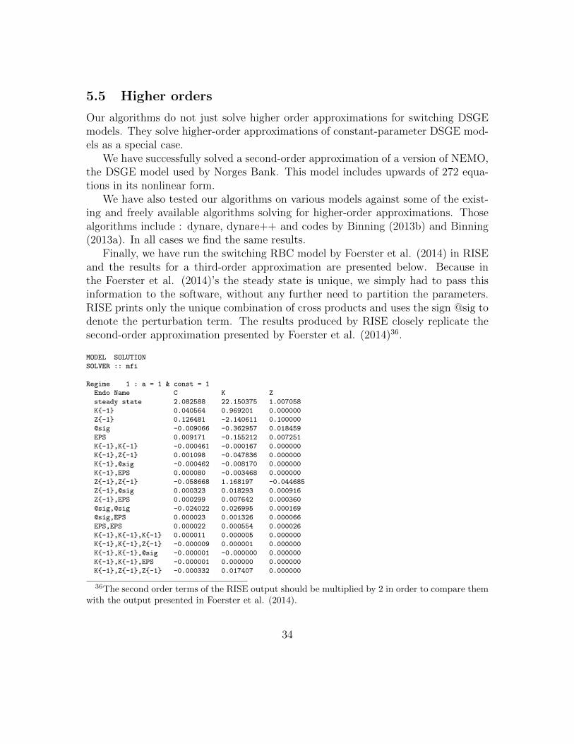
5.5 Higher orders

Our algorithms do not just solve higher order approximations for switching DSGEmodels. They solve higher-order approximations of constant-parameter DSGE mod-els as a special case.

We have successfully solved a second-order approximation of a version of NEMO,the DSGE model used by Norges Bank. This model includes upwards of 272 equa-tions in its nonlinear form.

We have also tested our algorithms on various models against some of the exist-ing and freely available algorithms solving for higher-order approximations. Thosealgorithms include : dynare, dynare++ and codes by Binning (2013b) and Binning(2013a). In all cases we find the same results.

Finally, we have run the switching RBC model by Foerster et al. (2014) in RISEand the results for a third-order approximation are presented below. Because inthe Foerster et al. (2014)’s the steady state is unique, we simply had to pass thisinformation to the software, without any further need to partition the parameters.RISE prints only the unique combination of cross products and uses the sign @sig todenote the perturbation term. The results produced by RISE closely replicate thesecond-order approximation presented by Foerster et al. (2014)36.

MODEL SOLUTION

SOLVER :: mfi

Regime 1 : a = 1 & const = 1

Endo Name C K Z

steady state 2.082588 22.150375 1.007058

K-1 0.040564 0.969201 0.000000

Z-1 0.126481 -2.140611 0.100000

@sig -0.009066 -0.362957 0.018459

EPS 0.009171 -0.155212 0.007251

K-1,K-1 -0.000461 -0.000167 0.000000

K-1,Z-1 0.001098 -0.047836 0.000000

K-1,@sig -0.000462 -0.008170 0.000000

K-1,EPS 0.000080 -0.003468 0.000000

Z-1,Z-1 -0.058668 1.168197 -0.044685

Z-1,@sig 0.000323 0.018293 0.000916

Z-1,EPS 0.000299 0.007642 0.000360

@sig,@sig -0.024022 0.026995 0.000169

@sig,EPS 0.000023 0.001326 0.000066

EPS,EPS 0.000022 0.000554 0.000026

K-1,K-1,K-1 0.000011 0.000005 0.000000

K-1,K-1,Z-1 -0.000009 0.000001 0.000000

K-1,K-1,@sig -0.000001 -0.000000 0.000000

K-1,K-1,EPS -0.000001 0.000000 0.000000

K-1,Z-1,Z-1 -0.000332 0.017407 0.000000

36The second order terms of the RISE output should be multiplied by 2 in order to compare themwith the output presented in Foerster et al. (2014).

34

K-1,Z-1,@sig 0.000005 0.000269 0.000000

K-1,Z-1,EPS 0.000002 0.000115 0.000000

K-1,@sig,@sig -0.000185 0.000231 0.000000

K-1,@sig,EPS 0.000000 0.000020 0.000000

K-1,EPS,EPS 0.000000 0.000008 0.000000

Z-1,Z-1,Z-1 0.037330 -0.811474 0.028102

Z-1,Z-1,@sig -0.000250 -0.006515 -0.000273

Z-1,Z-1,EPS -0.000097 -0.002777 -0.000107

Z-1,@sig,@sig -0.000418 -0.000480 0.000006

Z-1,@sig,EPS -0.000001 -0.000043 0.000002

Z-1,EPS,EPS 0.000001 -0.000018 0.000001

@sig,@sig,@sig -0.002111 0.001640 0.000001

@sig,@sig,EPS -0.000028 -0.000038 0.000000

@sig,EPS,EPS -0.000000 -0.000003 0.000000

EPS,EPS,EPS 0.000000 -0.000001 0.000000

Regime 2 : a = 2 & const = 1

Endo Name C K Z

steady state 2.082588 22.150375 1.007058

K-1 0.040564 0.969201 0.000000

@sig -0.100434 0.926307 -0.041021

EPS 0.026867 -0.464994 0.021752

K-1,K-1 -0.000461 -0.000167 0.000000

K-1,@sig -0.001160 0.020327 0.000000

K-1,EPS 0.000233 -0.010399 0.000000

@sig,@sig -0.023223 0.043449 0.000835

@sig,EPS -0.000525 -0.009756 -0.000443

EPS,EPS 0.000187 0.004982 0.000235

K-1,K-1,K-1 0.000011 0.000005 0.000000

K-1,K-1,@sig 0.000007 -0.000003 0.000000

K-1,K-1,EPS -0.000002 0.000000 0.000000

K-1,@sig,@sig -0.000188 0.000476 0.000000

K-1,@sig,EPS -0.000002 -0.000146 0.000000

K-1,EPS,EPS 0.000001 0.000075 0.000000

@sig,@sig,@sig -0.001411 0.002643 -0.000011

@sig,@sig,EPS -0.000077 -0.000228 0.000006

@sig,EPS,EPS -0.000002 0.000069 -0.000003

EPS,EPS,EPS 0.000001 -0.000036 0.000002

Finally we can use the same Foerster et al. (2014) model to illustrate in a third-order approximation, the effect of technology shock that is announced 4 periods fromnow. We compare two economies. In the first economy, agents fully anticipate theshock and therefore internalize their effect already in the current period. In thesecond economy, agents will be aware of the shock only when it will materialize 4periods from now. As figure 1 illustrates, consumption already increases today whilecapital falls in the ”anticipate” scenario.

6 Conclusion

In this paper we have proposed new solution algorithms for solving switching-parameterDSGE models. The algorithms developed are useful tools for analyzing economic

35

Figure 1: Third-order perturbation impulse responses to a TFP shock in theFRWZ2014 rbc model

36

data subject to breaks and shifts in a rational expectations environment, whereagents, while forming their expectations, explicitly take into account the probabil-ity of a regime shift. In the process we have derived higher-order perturbations ofswitching DSGE models in which the probability of switching can be endogenousand in which anticipated future events can affect the current behavior of economicagents.

Despite the many benefits of departing from the assumption of constant parame-ters, the techniques and the ideas of MSDSGE modeling have yet to be fully adoptedby many macroeconomists as is the case for constant-parameter DSGE models pop-ularized through Dynare. Two main reasons could potentially explain this. On theone hand such models are a lot more difficult to solve and more computationallyintensive than their constant-parameter counterparts and on the other hand, thereare not many flexible and easy-to-use tools that would allow economists unable orunwilling to write complex code to take full advantage of these techniques and ad-dress the current policy questions. By providing both efficient solution algorithmsand the implementation of those algorithms in a toolbox, we hope to have assuagedthese problems.

References

Adjemian, S., H. Bastani, M. Juillard, F. Karame, F. Mihoubi, G. Perendia,J. Pfeifer, M. Ratto, and S. Villemot (2011). Dynare: Reference manual, ver-sion 4. Dynare Working Papers 1, CEPREMAP.

Benner, P. and R. Byers (1998). An exact line search method for solving generalizedcontinuous-time algebraic riccati equations. IEEE Transactions on AutomaticControl 43 (1), 101–107.

Bernanke, B. S., M. Gertler, and S. Gilchrist (1999). The financial acceleratorin a quantitative business cycle framework. In J. B. T. . M. Woodford (Ed.),Handbook of Macroeconomics (1 ed.), Volume 1, Chapter 21, pp. 1341–1393.Elsevier.

Bi, H. and N. Traum (2013). Estimating fiscal limits: The case of greece. Journalof Applied Econometrics(forthcoming).

Binning, A. J. (2013a). Solving second and third-order approximations to dsgemodels: A recursive sylvester equation solution. Working Paper 2013—18,Norges Bank.

37

Binning, A. J. (2013b). Third-order approximation of dynamic models without theuse of tensors. Working Paper 2013—13, Norges Bank.

Buchberger, B. (1965). Ein Algorithmus zum Auffinden der Basiselemente desRestklassenringes nach einem nulldimensionalen Polynomideal. Ph. D. thesis,University of Innsbruck.

Buchberger, B. (2006, March). An Algorithm for Finding the Basis Elements inthe Residue Class Ring Modulo a Zero Dimensional Polynomial Ideal. Ph. D.thesis, RISC (Research Institute for Symbolic Computation),Johannes KeplerUniversity Linz.

Cho, S. (2014, February). Characterizing markov-switching rational expectationmodels. Working paper, Yonsei University.

Cogley, T., T. J. Sargent, and P. Surico (2012, March). The return of the gibsonparadox. Working paper, New York University.

Costa, O. L. D. V., M. D. Fragoso, and R. P. Marques (2005). Discrete-TimeMarkov Jump Linear Systems. Springer.

Davig, T. and E. M. Leeper (2007). Fluctuating macro policies and the fiscal the-ory. In NBER Macroeconomics Annual 2007, Volume 21, pp. 247–316. NationalBureau of Economic Research.

Davig, T., E. M. Leeper, and T. B. Walker (2011). Inflation and the fiscal limit.European Economic Review 55 (1), 31–47.

Farmer, R. F., D. F. Waggoner, and T. Zha (2008). Minimal state variable solutionsto markov switching rational expectations models. Working Paper 2008-23,Federal Reserve Bank of Atlanta.

Farmer, R. F., D. F. Waggoner, and T. Zha (2011). Minimal state variable solu-tions to markov switching rational expectations models. Journal of EconomicsDynamics and Control 35 (12), 2150–2166.

Foerster, A., J. Rubio-Ramirez, D. Waggoner, and T. Zha (2013). Perturbationmethods for markov-switching models. Working Paper 2013-1, Federal ReserveBank of Atlanta.

Foerster, A., J. Rubio-Ramirez, D. Waggoner, and T. Zha (2014). Perturbationmethods for markov-switching models. Working Paper 20390, National Bureauof Economic Research.

Freund, R. W. (1993). A transpose-free quasi-minimal residual algorithm for non-hermitian linear systems. SIAM Journal of Scientific Computing 2 (14), 470–482.

38

Ghorbal, K., A. Sogokon, and A. Platzer (2014). Invariance of conjunctions of poly-nomial equalities for algebraic differential equations. Lecture Notes in Com-puter Science 8723, 151–167.

Gupta, V., R. Murray, and B. Hassibi (2003). On the control of jump linear markovsystems with markov state estimation. In Proceedings of the 2003 AmericanAutomatic Control Conference, pp. 2893–2898.

Juillard, M. and J. Maih (2010). Estimating dsge models with observed real-timeexpectation data. Technical report, Norges Bank.

Justiniano, A. and G. E. Primiceri (2008). The time-varying volatility of macroe-conomic fluctuations. American Economic Review 98 (3), 604–41.

Kamenik, O. (2005, February). Solving sdge models: A new algorithm for thesylvester equation. Computational Economics 25 (1), 167–187.

Klein, P. (2000). Using the generalized schur form to solve a multivariate linearrational expectations model. Journal of Economic Dynamics and Control 24,1405–1423.

Lanczos, C. (1952). Solution of systems of linear equations by minimized iterations.Journal of Research of the National Bureau of Standards 49, 33–53.

Levintal, O. (2014). Fifth order perturbation solution to dsge models. Workingpaper, Interdisciplinary Center Herzliya (IDC), School of Economics.

Leykin, A. (2004). On parallel computation of grobner bases. In ICPP Workshops,pp. 160–164.

Lubik, T. A. and F. Schorfheide (2004, March). Testing for indeterminacy: Anapplication to u.s. monetary policy. American Economic Review 94 (1), 190–217.

Maih, J. (2010). Conditional forecasts in dsge models. Working Paper 2010—07,Norges Bank.

Mayr, E. W. and A. R. Meyer (1982). The complexity of the word problemsfor commutative semigroups and polynomial ideals. Advances in Mathemat-ics 46 (3), 305–329.

Richter, A. W., N. A. Throckmorton, and T. B. Walker (2014, December). Ac-curacy speed and robustness of policy function iteration. Computational Eco-nomics 44 (4), 445–476.

39

Schmitt-Grohe, S. and M. Uribe (2004). Solving dynamic general equilibrium mod-els using a second-order approximation to the policy function. Journal of Eco-nomics Dynamics and Control 28, 755–775.

Sims, C. A. and T. Zha (2006). Were there regime switches in us monetary policy?American Economic Review 96 (1), 54–81.

Smets, F. and R. Wouters (2007). Shocks and frictions in us business cycles: Abayesian dsge approach. American Economic Review, American Economic As-sociation 97 (3), 586–606.

Stock, J. H. and M. W. Watson (2003). Has the business cycle changed? evidenceand explanations. FRB Kansas City symposium, Jackson Hole.

Svensson, L. E. O. and N. Williams (2007). Monetary policy with model un-certainty: Distribution forecast targeting. CEPR Discussion Papers 6331,C.E.P.R.

Svensson, L. E. O. and N. Williams (2009). Optimal monetary policy underuncertainty in dsge models: A markov jump-linear-quadratic approach. InK. Schmidt-Hebbel, C. E. Walsh, and N. Loayza (Eds.), Central Banking,Analysis, and Economic Policies (1 ed.), Volume 13 of Monetary Policy underUncertainty and Learning, pp. 077–114. Central Bank of Chile.

Tadonki, C. and B. Philippe (1999). Parallel multiplication of a vector bya kronecker product of matrices. Parallel Distributed Computing PracticesPDCP 2 (4).

Van Loan, C. F. (2000). The ubiquitous kronecker product. Journal of Computa-tional and Applied Mathematics 123 (123), 85–100.

A Expressions for various expectations terms

A.1 First order

The definitions of a0z and a1

z appearing in equation (10) are as follows

a0z ≡

λbfT rt+1z hrtzT rtzmp

mb

mε,0

θrt+1mσ

40

a1z ≡

(λbfT rt+1

z

0(ns+2np+2nb+nf+nε+nθ)×nz

)We have

Evz = a0z (35)

A.2 Second order

hrtzz =

[λxT rtzz

0(1+(k+1)nε)×n2z

](36)

The definitions of a0zz and a1

zz appearing in equation (19) are as follows:

a0zz ≡

λbfT rt+1z,x λxT rtzz + λbfT rt+1

zz (hrtz )⊗2

T rtzz0(nx+nε+nθ)×n2

z

a1zz ≡

λbfT rt+1zz

00

It follows that

Evzz ≡ a0zz + a1

zzEu⊗2 (37)

and

Ev⊗2z = (a0

z)⊗2

+ (a1z)⊗2Eu⊗2 (38)

The definition of u in (4) implies that37

E (u⊗2) =

[0(np+nb+1+knε)

2×n2z

~Inε (mσ ⊗mσ)

]37In general, we will have E

(u⊗k

)=

[0(np+nb+1+knε)

k×nkz

vec (Mk)m⊗kσ

], where Mk is the tensor of the

k-order moments of εt. This expression should be cheap to compute since mσ is a sparse vector.

41

A.3 Third order

The definitions of a0zz and a1

zz appearing in equation (21) are as follows:

a0zzz ≡

λbfT rt+1zzz (hrtz )⊗3 + ω1 (λbfT rt+1

zz (hrtz ⊗ hrtzz)) + λbfT rt+1z hrtzzz

T rtzzz0(nx+nε+nθ)×n3

z

(39)

a1zzz ≡

(λbfT rt+1

zzz

0(nT+nx+nε+nθ)×n3z

)(40)

where

hrtzzz =

[λxT rtzzz

0(1+(k+1)nε)×n3z

]

∂3T rt+1 (hrt (z)+uz)∂z3

= T rt+1zzz (hrtz )⊗3 + ω1 (T rt+1

zz (hrtz ⊗ hrtzz)) + T rt+1z,x λxT rtzzz+

T rt+1zzz u⊗3 + ω1 (T rt+1

zz (u⊗ hrtzz)) +

T rt+1zzz

[P((hrtz )⊗2 ⊗ u

)+ P (hrtz ⊗ u⊗2)

]We have

Evzzz = a0zzz + a1

zzzP(hrtz ⊗ Eu⊗2

)+ a1

zzzEu⊗3 (41)

We also need E (v⊗3z ), E (vz ⊗ vzz). Using (19) and (10), those quantities are

computed as

Ev⊗3z = (a0

z)⊗3

+ Ea0z ⊗ (a1

zu)⊗2

+

E (a1zu)⊗2 ⊗ a0

z + E (a1zu)⊗ a0

z ⊗ (a1zu) + E (a1

zu)⊗3 (42)

E (vz ⊗ vzz) = a0z ⊗ a0

zz + (a1z ⊗ a1

zz) (Eu⊗2 ⊗ hrtz + E (u⊗ hrtz ⊗ u)) +a0z ⊗ a1

zzEu⊗2 + (a1

z ⊗ a1zz)Eu

⊗3 (43)

B Proof of local convergence of functional itera-

tion

Before proving the theorem we first present a perturbation lemma that will facilitatethe subsequent derivations.

Lemma 3 Perturbation Lemma: Let Ξ be a non-singular matrix. If Ω is such that

‖Ξ−1‖ ‖Ω‖ < 1, then∥∥(Ξ + Ω)−1

∥∥ ≤ ‖Ξ−1‖1−‖Ξ−1‖‖Ω‖

42

Proof. We have(Ξ + Ω)−1 = [Ξ (I + Ξ−1Ω)]

−1

=[∑∞

i=0 (−Ξ−1Ω)i]

Ξ−1

which implies that ∥∥(Ξ + Ω)−1∥∥ ≤ ∥∥∥∑∞i=0 (−Ξ−1Ω)

i∥∥∥ ‖Ξ−1‖

≤∑∞

i=0 ‖(−Ξ−1Ω)‖i ‖Ξ−1‖=

∑∞i=0 ‖(Ξ−1Ω)‖i ‖Ξ−1‖

= 11−‖(Ξ−1Ω)‖ ‖Ξ

−1‖

≤ ‖Ξ−1‖1−‖Ξ−1‖‖Ω‖

Now we can prove the theorem. Define

Ξrt ≡ A0rt +

h∑rt+1=1

A+rt,rt+1

T ∗rt+1

and

Ω(k−1)rt ≡

h∑rt+1=1

A+rt,rt+1

(T (k−1)rt+1

− T ∗rt+1

)which implies ∥∥∥Ω

(k−1)rt

∥∥∥ =∥∥∥∑h

rt+1=1A+rt,rt+1

(T

(k−1)rt+1 − T

(∗)rt+1

)∥∥∥≤ a+

∑hrt+1=1 prt,rt+1

∥∥∥T (k−1)rt+1 − T

(∗)rt+1

∥∥∥ (44)

Also, we can write

T(k)rt − T

(∗)rt =

[Ξ−1rt −

(A0rt +

∑hrt+1=1 A

+rt,rt+1

T(k−1)rt+1

)−1]A−rt

= −(A0rt +

∑hrt+1=1A

+rt,rt+1

T(k−1)rt+1

)−1

Ω(k−1)rt T

(∗)rt

−(

Ω(k−1)rt + Ξrt

)−1 [Ω

(k−1)rt

]T

(∗)rt

43

so that∥∥∥T (k)rt − T

(∗)rt

∥∥∥ ≤ ∥∥∥∥(Ω(k−1)rt + Ξrt

)−1∥∥∥∥∥∥∥[∑h

rt+1=1A+rt,rt+1

(T

(k−1)rt+1 − T

(∗)rt+1

)]∥∥∥ ∥∥∥T (∗)rt

∥∥∥=

∥∥∥T (∗)rt

∥∥∥∥∥∥∥(Ω(k−1)rt + Ξrt

)−1∥∥∥∥∥∥∥[∑h

rt+1=1 A+rt,rt+1

(T

(k−1)rt+1 − T

(∗)rt+1

)]∥∥∥≤

∥∥∥T (∗)rt

∥∥∥∥∥∥∥(Ω(k−1)rt + Ξrt

)−1∥∥∥∥ a+

∑hrt+1=1

∥∥∥(T (k−1)rt+1 − T

(∗)rt+1

)∥∥∥≤ θa+

∥∥∥∥(Ω(k−1)rt + Ξrt

)−1∥∥∥∥∑h

rt+1=1

∥∥∥(T (k−1)rt+1 − T

(∗)rt+1

)∥∥∥(45)

We can now use induction in the rest of the proof. Suppose∥∥∥T (0)

rt − T ∗rt∥∥∥ ≤ δ,

rt = 1, 2, ..., h. Then (44) implies∥∥∥Ω

(0)rt

∥∥∥ ≤ a+δ. Hence∥∥Ξ−1

rt

∥∥∥∥∥Ω(0)rt

∥∥∥ ≤ τa+δ. Note

that the requirement that τa+ (θ + δ) < 1 automatically implies that τa+δ < 1.

Therefore we can use the perturbation lemma to establish that

∥∥∥∥(Ω(0)rt + Ξrt

)−1∥∥∥∥ ≤

‖Ξ−1rt ‖

1−‖Ξ−1rt ‖

∥∥∥Ω(0)rt

∥∥∥ ≤ τ1−τa+δ . Plugging this result into (45) implies that

∥∥∥T (1)rt − T

(∗)rt

∥∥∥ ≤θa+τ

1−τa+δ∑h

rt+1=1

∥∥∥(T (0)rt+1 − T

(∗)rt+1

)∥∥∥, essentially defining ϕ ≡ θa+τ1−τa+δ and saying that the

proposition holds for k = 1.Now suppose that the proposition holds for some arbitrary order k, that is∥∥∥T (k)rt − T ∗rt

∥∥∥ ≤ ϕ∑h

rt+1=1

∥∥∥T (k−1)rt+1 − T ∗rt+1

∥∥∥. We now have to show that it also holds

for order k + 1. Since by assumption∥∥∥(T (k−1)

rt+1 − T ∗rt+1

)∥∥∥ ≤ δ, for rt = 1, 2, ..., h, we

have∥∥∥T (k)

rt − T ∗rt∥∥∥ ≤ ϕ

∑hrt+1=1

∥∥∥T (k−1)rt+1 − T ∗rt+1

∥∥∥ ≤ ϕδ ≤ δ. (44) implies∥∥∥Ω

(k)rt

∥∥∥ ≤a+δ. Then by the perturbation lemma, if follows that

∥∥∥∥(Ω(k)rt + Ξrt

)−1∥∥∥∥ ≤ τ

1−τa+δ .

This implies by (45) that∥∥∥T (k+1)rt − T (∗)

rt

∥∥∥ ≤ θa+

∥∥∥∥(Ω(k)rt + Ξrt

)−1∥∥∥∥∑h

rt+1=1

∥∥∥(T (k)rt+1 − T

(∗)rt+1

)∥∥∥≤ θa+τ

1−τa+δ∑h

rt+1=1

∥∥∥(T (k)rt+1 − T

(∗)rt+1

)∥∥∥. And so, the proposition also holds at order k + 1.

44

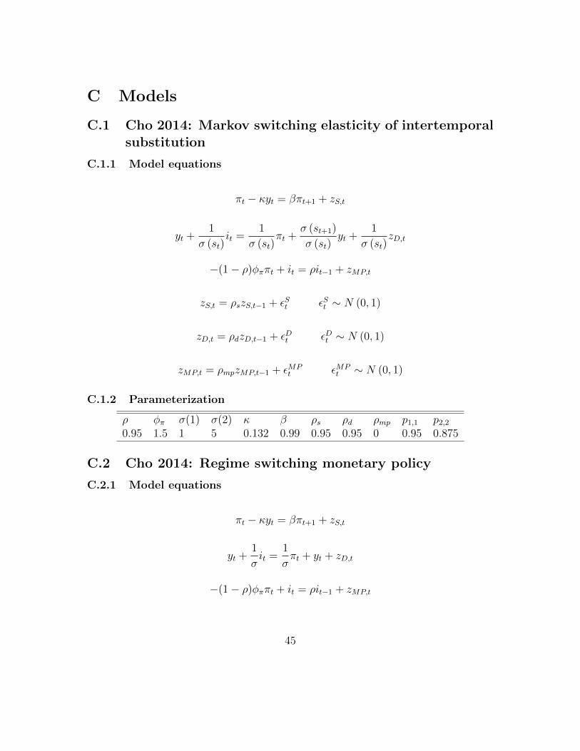
C Models

C.1 Cho 2014: Markov switching elasticity of intertemporalsubstitution

C.1.1 Model equations

πt − κyt = βπt+1 + zS,t

yt +1

σ (st)it =

1

σ (st)πt +

σ (st+1)

σ (st)yt +

1

σ (st)zD,t

−(1− ρ)φππt + it = ρit−1 + zMP,t

zS,t = ρszS,t−1 + εSt εSt ∼ N (0, 1)

zD,t = ρdzD,t−1 + εDt εDt ∼ N (0, 1)

zMP,t = ρmpzMP,t−1 + εMPt εMP

t ∼ N (0, 1)

C.1.2 Parameterization

ρ φπ σ(1) σ(2) κ β ρs ρd ρmp p1,1 p2,2

0.95 1.5 1 5 0.132 0.99 0.95 0.95 0 0.95 0.875

C.2 Cho 2014: Regime switching monetary policy

C.2.1 Model equations

πt − κyt = βπt+1 + zS,t

yt +1

σit =

1

σπt + yt + zD,t

−(1− ρ)φππt + it = ρit−1 + zMP,t

45

zS,t = ρszS,t−1 + εSt εSt ∼ N (0, 1)

zD,t = ρdzD,t−1 + εDt εDt ∼ N (0, 1)

zMP,t = ρmpzMP,t−1 + εMPt εMP

t ∼ N (0, 1)

C.2.2 Parameterization

ρ φπ(1) φπ(2) σ κ β ρs ρd ρmp p1,1 p2,2

0.95 0.9 1.5 1 0.132 0.99 0 0 0 0.85 0.95

C.3 Farmer, Waggoner and Zha (2011)

C.3.1 Model equations

φπt = πt+1 + δπt−1 + βrt

r = ρrt−1 + εt εt ∼ N (0, 1)

C.3.2 Parameterization

δ (1) δ (2) β (1) β (2) ρ (1) ρ (2) φ (1) φ (2) p1,1 p2,2

parameterization 1 0 0 1 1 0.9 0.9 0.5 0.8 0.8 0.9parameterization 2 -0.7 0.4 1 1 0 0 0.5 0.8 0 0.64parameterization 3 -0.7 -0.2 1 1 0 0 0.2 0.4 0.9 0.8

C.4 Foerster, Rubio-Ramirez, Waggoner and Zha (2014):RBC model

C.4.1 Model equations

cυ−1t = βzυ−1

t cυ−1t+1 (αz1−α

t+1 kα−1t + 1− δ)

ct + ztkt = z1−αt kαt−1 + (1− δ)kt−1

46

log(zt) = (1− ρ (st))µ (st) + ρ (st) log(zt−1) + σ (st) εt εt ∼ N (0, 1)

C.4.2 steady state

zt = exp (µ)

kt =

[1

αz1−αt

(1

βzυ−1t

− 1 + δ

)] 1α−1

ct = z1−αt kαt + (1− δ) kt − ztkt

C.4.3 Parameterization

α β υ δ µ(1) µ(2) ρ(1) ρ(2) σ(1) σ(2) p1,1 p2,2

0.33 0.9976 -1 0.025 0.0274 -0.0337 0.1 0 0.0072 0.0216 0.75 0.5

C.5 Foerster, Rubio-Ramirez, Waggoner and Zha (2013):NK model

C.5.1 Model equations

1− βEt(1− κ

2(πt − 1)2)Yt(

1− κ2

(πt+1 − 1)2)Yt+1

1

exp (µt+1)

Rt

πt+1

= 0

(1− η)+η(

1− κ

2(πt − 1)2

)Yt+βκEt

(1− κ

2(πt − 1)2)(

1− κ2

(πt+1 − 1)2) (πt+1 − 1) πt+1−κ (πt − 1) πt = 0

(Rt−1

Rss

)ρπ

(1−ρ)ψtt exp (σεt)− Rt

Rss= 0 εt ∼ N (0, 1)

C.5.2 Steady state solution

πt yt Rt

1 η−1η

exp(µ)β

πt

47

C.5.3 Parameterization

β κ η ρr σr p1,1 p2,2 µ (1) µ (2) ψ (1) ψ (2)0.9976 161 10 0.8 0.0025 0.9 0.9 0.0075 0.0025 3.1 0.9

C.6 Foerster, Rubio-Ramirez, Waggoner and Zha (2013):NK model with habits

C.6.1 Model equations

1

Ct − ϕ exp (−µ)Ct−1

− β ϕ

Xt+1 exp (µt+1)− ϕCt− λt = 0

βλt+1

exp(µt+1)

Rssπψtt exp(σεt)

πt+1− λt = 0 εt ∼ N (0, 1)

(1− η) +η

λt+ βκ(πt+1 − 1)πt+1

λt+1

λt

Xt+1

Ct

1− κ2(πt − 1)2

1− κ2(πt+1 − 1)2

− κ(πt − 1)πt

Xt − Ct

C.6.2 steady state

πt λt Xt Ct1 η

η−1exp(µ)−βϕexp(µ)−ϕ

η−1η

Xt

C.6.3 Parameterization

β κ η ρr σ p1,1 p2,2 µ (1) µ (2) ψ (1) ψ (2) Rss ϕ

0.9976 161 10 0.8 0.0025 0.9 0.9 0.0075 0.0025 3.1 0.9 exp(µ)β

0.7

C.7 The Smets-Wouters model with switching monetary pol-icy

We consider a medium scale DSGE model by Smets and Wouters (2007). We turnit into a Markov switching model by introducing a Markov chain in two regimes,controlling the behavior of the parameters entering the monetary policy reactionfunction. In the good regime, the parameters assume the mode values estimated bySmets and Wouters (2007) for the constant parameter case. In the bad regime the

48

interest rate is unresponsive to inflation and output gap. However, the interest rate isallowed to respond to a persistent exogenous monetary policy shock and is thereforeexogenous. In a constant-parameter model, this bad regime would be unstable. Ina switching environment, however, to the extent that agents assign a sufficientlyhigh probability to the system returning to the good regime, the system may bestable in the MSS sense. The table below displays the parameters: rπ is the reactionto inflation; ρ, the smoothing parameter; ry, the reaction to output gap; r∆y, thereaction to the change in output gap; pgood,good is the probability of remaining in thegood regime; pbad,bad is the probability of remaining in the bad regime.

rπ ρ ry r∆y pgood,good pbad,badGood regime 1.4880 0.8762 0.0593 0.2347 0.9 NABad regime 0.0000 0.0000 0.0000 0.0000 NA 0.3

49