Dynamical correlations of S = 1 2 quantum spin chainsiaffleck/per-the.pdf · Dynamical correlations of S = 1/2 quantum ... acting spins that behave according to the rules of quantum

Dynamical correlations of S = 1/2 quantum

spin chains

by

Rodrigo G. Pereira

B.Sc., State University of Campinas, Brazil, 2002M.Sc., State University of Campinas, Brazil, 2004

A THESIS SUBMITTED IN PARTIAL FULFILMENT OFTHE REQUIREMENTS FOR THE DEGREE OF

DOCTOR OF PHILOSOPHY

in

The Faculty of Graduate Studies

(Physics)

THE UNIVERSITY OF BRITISH COLUMBIA

April 2008

c© Rodrigo G. Pereira 2008

ii

Abstract

The genthesis.cls LATEX class file and accompanying documents, such asthis sample thesis, are distributed in the hope that it will be useful butwithout any warranty (without even the implied warranty of fitness for aparticular purpose). For a description of this file’s purpose, and instructionson its use, see below.

These files are distributed under the GPL which should be included herein the future. Please let the author know of any changes or improvementsthat should be made.

Michael Forbes. [email protected]

iii

Table of Contents

Abstract . . . . . . . . . . . . . . . . . . . . . . . . . . . . . . . . . . ii

Table of Contents . . . . . . . . . . . . . . . . . . . . . . . . . . . . iii

List of Tables . . . . . . . . . . . . . . . . . . . . . . . . . . . . . . iv

List of Figures . . . . . . . . . . . . . . . . . . . . . . . . . . . . . . v

Acknowledgements . . . . . . . . . . . . . . . . . . . . . . . . . . . vi

1 Introduction . . . . . . . . . . . . . . . . . . . . . . . . . . . . . 11.1 Heisenberg model . . . . . . . . . . . . . . . . . . . . . . . . 21.2 An example of a Heisenberg spin chain . . . . . . . . . . . . . 31.3 The Bethe ansatz . . . . . . . . . . . . . . . . . . . . . . . . 41.4 Anisotropic spin chains . . . . . . . . . . . . . . . . . . . . . 71.5 Field theory methods . . . . . . . . . . . . . . . . . . . . . . 101.6 The problem of dynamical correlation functions . . . . . . . . 131.7 Beyond the Luttinger liquid paradigm . . . . . . . . . . . . . 171.8 Overview . . . . . . . . . . . . . . . . . . . . . . . . . . . . . 21

Bibliography . . . . . . . . . . . . . . . . . . . . . . . . . . . . . . . 23

2 Broadening of the dynamical structure factor . . . . . . . . 282.1 Another Section . . . . . . . . . . . . . . . . . . . . . . . . . 28

3 High-frequency tail . . . . . . . . . . . . . . . . . . . . . . . . . 29

4 Edge singularities and long-time decay . . . . . . . . . . . . . 30

iv

List of Tables

v

List of Figures

1.1 Spin chain. . . . . . . . . . . . . . . . . . . . . . . . . . . . . . 21.2 Sr2CuO3. . . . . . . . . . . . . . . . . . . . . . . . . . . . . . 51.3 Phase diagram for XXZ model in a field. . . . . . . . . . . . . 91.4 Dynamical structure factor for the XY model. . . . . . . . . . 141.5 Muller ansatz vs exact two-spinon result. . . . . . . . . . . . . 18

vi

Acknowledgements

This is the place to thank professional colleagues and people who have givenyou the most help during the course of your graduate work.

1

Chapter 1

Introduction

Quantum spin chains provide simple yet rich examples of strongly correlatedsystems. For a theoretical physicist, one-dimensional (1D) arrays of inter-acting spins that behave according to the rules of quantum mechanics areinteresting because they are amenable to detailed analytical and numericalstudies [1]. These studies have revealed that spin chains exhibit exotic prop-erties which contradict our classical intuition about magnetic ordering. Forinstance, spin-1/2 chains with an isotropic antiferromagnetic exchange in-teraction do not order even at zero temperature, and their spectrum is bestinterpreted in terms of fractional excitations named spinons which are verydifferent from spin waves in three-dimensional magnets. But spin chains arenot confined to the theoretical realm. They also exist in the real world, inthe form of chemical compounds in which, due to the lattice structure, thecoupling between magnetic ions is highly anisotropic and strongest along onespatial direction [2]. Indeed, thanks to steady advances in materials science,the research field of 1D quantum magnetism has benefited from the interplaybetween theory and experiment that is essential in condensed matter physics.The interest in spin chain models is actually quite general, ranging from ap-plications in quantum computation [3] to mathematical tools in string theory[4].

Given the long history of studies of spin chains, it is fair to say that mostrelevant static thermodynamic properties, such as specific heat and magneticsusceptibility, are well understood by now. However, despite various efforts,the problem of calculating dynamical properties, such as the dynamical struc-ture factor probed directly in inelastic neutron scattering experiments, posesa challenge to standard theoretical approaches and has remained unsolved.The need to clarify some of the open questions concerning the dynamics ofspin chains motivated the work reported in this thesis.

Chapter 1. Introduction 2

1.1 Heisenberg model

Electrons are charged spin-1/2 particles which carry an intrinsic magneticmoment. In the early days of quantum mechanics, Werner Heisenberg [5]pointed out that the spin-independent Coulomb interaction between twoelectrons in a diatomic molecule, with a properly anti-symmetrized wavefunction, gives rises to an exchange interaction that couples the electronspins. The generalization of this idea to a large number of electrons leads toan important mechanism for magnetism in solids [2]. The Heisenberg modeldescribes a bilinear exchange interaction between nearest neighbor spins atfixed positions on a lattice

H = J∑

〈ij〉

~Si · ~Sj (1.1)

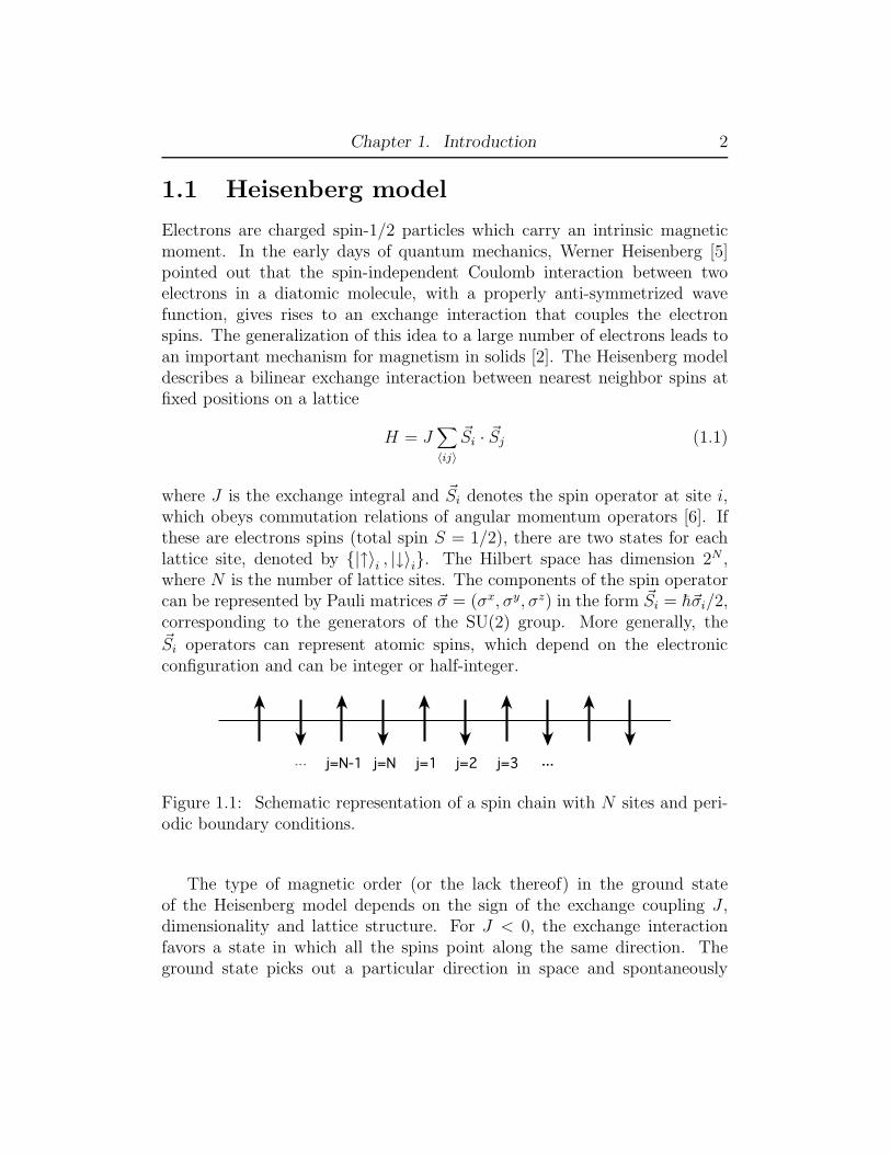
where J is the exchange integral and ~Si denotes the spin operator at site i,which obeys commutation relations of angular momentum operators [6]. Ifthese are electrons spins (total spin S = 1/2), there are two states for eachlattice site, denoted by {|↑〉i , |↓〉i}. The Hilbert space has dimension 2N ,where N is the number of lattice sites. The components of the spin operatorcan be represented by Pauli matrices ~σ = (σx, σy, σz) in the form ~Si = h~σi/2,corresponding to the generators of the SU(2) group. More generally, the~Si operators can represent atomic spins, which depend on the electronicconfiguration and can be integer or half-integer.

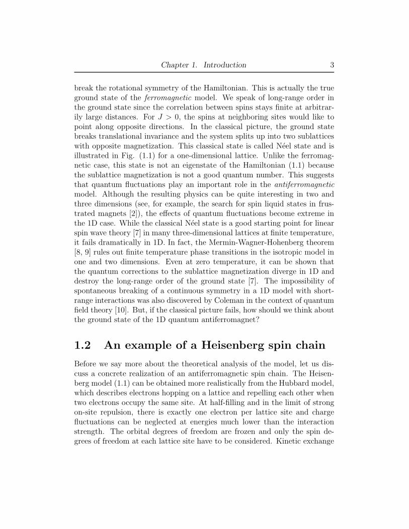
j=1 j=2j=N-1 j=3... ...j=N

Figure 1.1: Schematic representation of a spin chain with N sites and peri-odic boundary conditions.

The type of magnetic order (or the lack thereof) in the ground stateof the Heisenberg model depends on the sign of the exchange coupling J ,dimensionality and lattice structure. For J < 0, the exchange interactionfavors a state in which all the spins point along the same direction. Theground state picks out a particular direction in space and spontaneously


break the rotational symmetry of the Hamiltonian. This is actually the trueground state of the ferromagnetic model. We speak of long-range order inthe ground state since the correlation between spins stays finite at arbitrar-ily large distances. For J > 0, the spins at neighboring sites would like topoint along opposite directions. In the classical picture, the ground statebreaks translational invariance and the system splits up into two sublatticeswith opposite magnetization. This classical state is called Neel state and isillustrated in Fig. (1.1) for a one-dimensional lattice. Unlike the ferromag-netic case, this state is not an eigenstate of the Hamiltonian (1.1) becausethe sublattice magnetization is not a good quantum number. This suggeststhat quantum fluctuations play an important role in the antiferromagnetic

model. Although the resulting physics can be quite interesting in two andthree dimensions (see, for example, the search for spin liquid states in frus-trated magnets [2]), the effects of quantum fluctuations become extreme inthe 1D case. While the classical Neel state is a good starting point for linearspin wave theory [7] in many three-dimensional lattices at finite temperature,it fails dramatically in 1D. In fact, the Mermin-Wagner-Hohenberg theorem[8, 9] rules out finite temperature phase transitions in the isotropic model inone and two dimensions. Even at zero temperature, it can be shown thatthe quantum corrections to the sublattice magnetization diverge in 1D anddestroy the long-range order of the ground state [7]. The impossibility ofspontaneous breaking of a continuous symmetry in a 1D model with short-range interactions was also discovered by Coleman in the context of quantumfield theory [10]. But, if the classical picture fails, how should we think aboutthe ground state of the 1D quantum antiferromagnet?

1.2 An example of a Heisenberg spin chain

Before we say more about the theoretical analysis of the model, let us dis-cuss a concrete realization of an antiferromagnetic spin chain. The Heisen-berg model (1.1) can be obtained more realistically from the Hubbard model,which describes electrons hopping on a lattice and repelling each other whentwo electrons occupy the same site. At half-filling and in the limit of strongon-site repulsion, there is exactly one electron per lattice site and chargefluctuations can be neglected at energies much lower than the interactionstrength. The orbital degrees of freedom are frozen and only the spin de-grees of freedom at each lattice site have to be considered. Kinetic exchange


that results from virtual hopping processes lifts the spin degeneracy of theground state and the low-energy effective model is the Heisenberg model withJ > 0 (antiferromagnetic) [2]. This means that antiferromagnetism appearsnaturally in Mott insulators, as is indeed observed in real compounds.

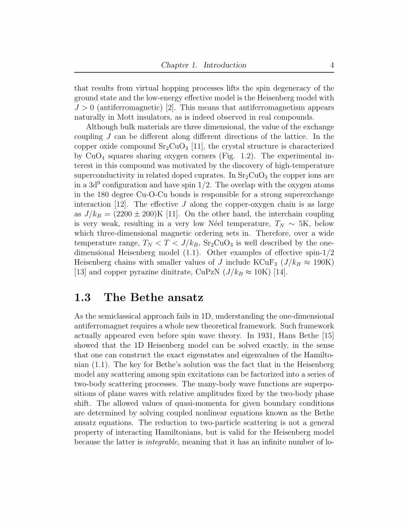
Although bulk materials are three dimensional, the value of the exchangecoupling J can be different along different directions of the lattice. In thecopper oxide compound Sr2CuO3 [11], the crystal structure is characterizedby CuO4 squares sharing oxygen corners (Fig. 1.2). The experimental in-terest in this compound was motivated by the discovery of high-temperaturesuperconductivity in related doped cuprates. In Sr2CuO3 the copper ions arein a 3d9 configuration and have spin 1/2. The overlap with the oxygen atomsin the 180 degree Cu-O-Cu bonds is responsible for a strong superexchangeinteraction [12]. The effective J along the copper-oxygen chain is as largeas J/kB = (2200 ± 200)K [11]. On the other hand, the interchain couplingis very weak, resulting in a very low Neel temperature, TN ∼ 5K, belowwhich three-dimensional magnetic ordering sets in. Therefore, over a widetemperature range, TN < T < J/kB, Sr2CuO3 is well described by the one-dimensional Heisenberg model (1.1). Other examples of effective spin-1/2Heisenberg chains with smaller values of J include KCuF3 (J/kB ≈ 190K)[13] and copper pyrazine dinitrate, CuPzN (J/kB ≈ 10K) [14].

1.3 The Bethe ansatz

As the semiclassical approach fails in 1D, understanding the one-dimensionalantiferromagnet requires a whole new theoretical framework. Such frameworkactually appeared even before spin wave theory. In 1931, Hans Bethe [15]showed that the 1D Heisenberg model can be solved exactly, in the sensethat one can construct the exact eigenstates and eigenvalues of the Hamilto-nian (1.1). The key for Bethe’s solution was the fact that in the Heisenbergmodel any scattering among spin excitations can be factorized into a series oftwo-body scattering processes. The many-body wave functions are superpo-sitions of plane waves with relative amplitudes fixed by the two-body phaseshift. The allowed values of quasi-momenta for given boundary conditionsare determined by solving coupled nonlinear equations known as the Betheansatz equations. The reduction to two-particle scattering is not a generalproperty of interacting Hamiltonians, but is valid for the Heisenberg modelbecause the latter is integrable, meaning that it has an infinite number of lo-


Cu

O

Sr

c

b

a

(a) Crystal structure of Sr2CuO3, a S = 1/2 Heisenberg chaincompound. Adapted from Ref. [11].

b

c

(b) A cut on the bc plane showing the Cu-O chain. The chain oxygensmediate a superexchange interaction between the magnetic copper ions.

Figure 1.2:


cal conserved quantities.1 Remarkably, integrability is not so unusual in onedimension. Other widely studied 1D models, such as the Lieb-Liniger model[17] (interacting Bose gas) and the Hubbard model [18], are also integrable.The Bethe ansatz is also applicable to these models.

The Bethe ansatz solution [19, 20] proves that the ground state of thespin-1/2 Heisenberg chain is unique and has total spin equal to zero (a singletstate) if the number of sites is even. The spectrum is gapless (or “massless”)in the thermodynamic limit. The elementary excitation is called a spinonand corresponds to a hole in the set of roots of the Bethe ansatz equations.A single spinon is a fractional excitation which carries spin 1/2 and cannotbe created alone without changing the boundary conditions. In order forthe total Sz of the chain to change by an integer number, as required bysuperselection rules, the spinons have to be created in pairs. This implies,for instance, that the simplest triplet excitation lie in a two-parameter con-tinuum (whose lower bound is known as the de Cloizeaux-Pearson dispersion[21]), in contrast with the single-magnon peak predicted by semiclassical spinwave theory. This has in fact been observed in inelastic neutron scatteringexperiments [14], in a clear demonstration of one-dimensional behavior.

The Bethe ansatz equations for the Heisenberg spin-1/2 chain have beenextensively studied, in an attempt to extract useful properties of the model.Due to the complexity of the solution, this is not always possible. It sufficesto say that, seventy seven years after the original paper, not even the com-pleteness of the Bethe eigenstates for the XXZ model (without an assumptionabout the distribution of complex roots known as the string hypothesis) hasbeen proved yet [22]. In the thermodynamic limit, the Bethe ansatz equa-tions assume the form of integral equations for the density of quasi-momenta.Some exact results which have been obtained by manipulating these equa-tions include the ground state energy [23], zero temperature susceptibility [24]and spin wave velocity [21]. An application of the Bethe ansatz equationsfor finite systems is the calculation of the finite size spectrum [25], which isimportant in conformal field theory [26]. It is also possible to compute finitetemperature static properties (e.g. specific heat, finite temperature suscepti-bility) using a set of nonlinear integral equations known as Thermodynamic

1Actually, the definition of integrability is clear for classical models, but ambiguous inquantum mechanics because linearly independent conserved quantities can be constructedfor any quantum model (see discussion in [16]). It is more useful to think of quantumintegrability as the absence of diffraction or three-particle scattering, as is the case for theBethe ansatz solvable models.


Bethe Ansatz (TBA) [27]. However, this procedure has been criticized forrelying on the string hypothesis to describe the spectrum of the XXZ model.

It is worth mentioning that models describing spin chains with highervalues of S are not integrable. The case S = 1/2 is therefore special sincewe have access to an exact solution with which approximate analytical andnumerical results can be compared. However, according to the Lieb-Shultz-Mattis theorem [28], a gapless spectrum is generic in isotropic half-integerspin chains, unless parity symmetry is spontaneously broken and the groundstate is degenerate. The theorem does not hold for integer values of S.In fact, Haldane [29] conjectured that integer spin chains should exhibita finite gap to the lowest excited state, while the SU(2) symmetry remainsunbroken. Haldane’s conjecture has been confirmed by numerical calculationsas well as experimentally, and the existence of a gap was proven rigorously forthe related bilinear biquadratic S = 1 Affleck-Kennedy-Lieb-Tasaki (AKLT)model [30]. The difference between integer and half-integer spin chains canbe attributed to the effects of a topological term in the nonlinear sigma model[31].

1.4 Anisotropic spin chains

The generalization of the model (1.1) which introduces exchange anisotropyas well as a finite external magnetic field is the so-called XXZ model in afield

H = JN

∑

j=1

[Sxj Sx

j+1 + Syj S

yj+1 + ∆Sz

j Szj+1 − hSz

j ]. (1.2)

In comparison with the Heisenberg (or XXX) model, the symmetry of theXXZ model has been reduced from SU(2) to U(1) (rotation around the zaxis). The total magnetization Sz =

∑

j Szj is still a good quantum number.

Moreover, this model is also integrable by the Bethe ansatz [32, 33]. Whilesome exact analytical results can be derived for the model with h = 0, ingeneral the Bethe ansatz equations for the XXZ model at finite magneticfield have to be solved numerically [19].2

The first reason to study the XXZ model is that one should not expectperfectly isotropic exchange interactions in real materials. On a lattice the

2A simple program to solve the Bethe ansatz equations for the XXZ model numericallycan be found in the appendix of Ref. [1].


rotational symmetry of the spin interaction can be broken by spin-orbit ordipolar interactions. However, this effect is weak and bulk spin chain materi-als are very close to being isotropic [34]. But the second and most importantreason why the XXZ model is interesting is because it appears as an effectivemodel whenever a physical system can be described as a one-dimensional lat-tice with two states per site. One example is that of S = 1/2 two-leg laddersin the strong coupling limit J⊥ ≫ J‖, where J⊥ and J‖ are the couplingsalong the rungs and along the chain, respectively [35]. Two-leg ladders aresimilar to S = 1 chains in the sense that there is an energy gap to the tripletstate on each rung. But an external magnetic field can lower the energy ofthe triplet state with total Sz parallel to the field. Near the critical field, thesinglet-triplet gap closes and the two low-lying states form a doublet whichacts as an effective spin-1/2 degree of freedom. The effective model for aS = 1/2 ladder with J⊥ ≫ J‖ is the XXZ model with ∆ = 1/2 [36, 37]. Ar-tificial systems which have phases described by effective XXZ models, witharbitrary values of ∆, include Josephson junction arrays [38], linear arrays ofqubits [39] and ultracold bosonic atoms (with two internal hyperfine states)trapped in optical lattices [40]. In the latter, it should be even possible toobserve phenomena associated with the integrability of the 1D model, suchas the absence of relaxation mechanisms [41].

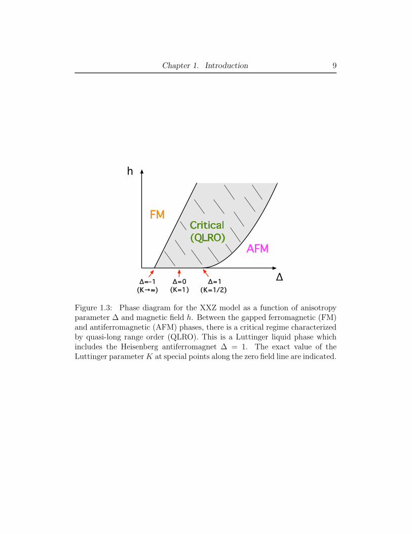
The Bethe ansatz solution allows us to map out the phase diagram of theXXZ model by looking at the energy of the low-lying excitations as a functionof exchange anisotropy ∆ and magnetic field h (Fig. 1.3). Along the zero fieldline in parameter space, the limits ∆ → −∞ and ∆ → +∞ correspond tothe classical Ising ferromagnet and antiferromagnet, respectively. These areboth known to have a gapped spectrum, with domain-wall-type excitations.We also know that the model is gapless at the Heisenberg point ∆ = 1, so weshould expect quantum phase transitions by simply varying the anisotropyparameter ∆. As a matter of fact, the Bethe ansatz reveals that the XXZchain is gapless along an entire critical line −1 < ∆ ≤ 1 (sometimes calledeasy plane anisotropy regime). There is a gapped ferromagnetic phase for∆ < −1 and a gapped Neel phase for ∆ > 1. Including the magnetic field,one finds the ground state phase diagram represented in Fig. 1.3 [16]. Thereis a whole region where the spectrum of the spin chain is gapless. Startingfrom the gapless phase, the system enters the ferromagnetic phase if the fieldis increased above the saturation field. On the other hand, a finite magneticfield can close the gap for ∆ > 1.

The gapped, Ising-like phases of the XXZ spin chain can be understood


h

Δ

Critical

(QLRO)

FM

AFM

Δ=1

(K=1/2)

Δ=0

(K=1)

Δ=-1

(K→∞)

Figure 1.3: Phase diagram for the XXZ model as a function of anisotropyparameter ∆ and magnetic field h. Between the gapped ferromagnetic (FM)and antiferromagnetic (AFM) phases, there is a critical regime characterizedby quasi-long range order (QLRO). This is a Luttinger liquid phase whichincludes the Heisenberg antiferromagnet ∆ = 1. The exact value of theLuttinger parameter K at special points along the zero field line are indicated.


with simple semiclassical pictures, but the gapless phase seems more exotic.Long-range order should not exist in this phase, which includes the Heisen-berg model. What we would really like to know in order to characterize thisphase and make connection with experiments is how spin-spin correlationfunctions decay at large distances. Unfortunately, this cannot be done byemploying directly the Bethe ansatz solution. Even when we know the ex-act eigenstates and the spectrum, calculating correlation functions requirescomputing matrix elements (so-called form factors) between a unmanageablenumber of complicated wave functions (recall that the size of Hilbert spacegrows as 2N). This calls for an alternative, approximate yet more intuitiveapproach to the physics of one-dimensional magnets.

1.5 Field theory methods

Another reason to consider the anisotropic model is that the XXZ spin chainis equivalent to a model of interacting spinless fermions. This is made clearby the Jordan-Wigner transformation, which maps the Sz

j operator onto alocal density of fermions [1]. This way, the spin-up state is equivalent toa particle and the spin-down state to a hole. Under this transformationthe x and y terms of the exchange interaction in (1.2) are mapped onto akinetic energy (hopping) term, whereas the z part translates into a density-density interaction term. As a result, the model with ∆ = 0, known as theXY model, is equivalent to free fermions on the lattice and can be solvedvery easily by performing a Fourier transform to momentum space. Theground state of the XY model is understood as a Fermi sea of the Jordan-Wigner fermions, whose density is fixed by the magnetization of the spinchain. In particular, the zero field case corresponds to a half-filled band,with one fermion per every other lattice site. Excitations with total Sz = 0correspond to the creation of particle-hole pairs. This solution of the XYmodel makes it possible to calculate some correlation functions exactly [28,42]. The correlation functions are found to decay very slowly (as power laws)in the large distance limit, which leads to the notion of quasi-long range order

in 1D gapless systems.The solution of the XY model also provides a convenient starting point

for exploring the entire gapless phase once we find a way to treat the fermion-fermion interactions for ∆ 6= 0. In three dimensions, Landau’s Fermi liquid


theory [43] shows that the excitations of a system of interacting fermions3 arequasiparticles which resemble the “bare” electron in the Fermi gas and differonly by the renormalization of a few parameters such as the effective mass[44]. The situation is very different in one dimension, because again quan-tum fluctuations have a drastic effect and lead to the breakdown of Fermiliquid theory in 1D [45]. The method of choice to describe the low-energyexcitations of an interacting 1D fermionic system is called bosonization [46].This approach starts by taking the continuum limit and linearizing the dis-persion of the particle-hole excitations about the Fermi points with momen-tum ±kF . One then introduces an effective bosonic field associated withthe collective density fluctuations of the Fermi gas. The advantage of thebosonization method is that “forward” fermionic interactions can be treatedexactly. Their effect is simply to renormalize the velocity and “stiffness” ofthe non-interacting bosons. The resulting free boson model is known as theLuttinger model [47]. There is no clear correspondence between the bosonsof the Luttinger model and the exact eigenstates found in the Bethe ansatz.However, it is possible to define a kink in the bosonic field that carries spin-1/2 and for ∆ = 1 obeys semionic statistics, in close analogy with the spinonsof the Heisenberg model [48].

The bosonization approach is asymptotically exact in the limit of lowenergies and long wavelengths. Haldane [49] introduced the concept of theLuttinger liquid, pointing out that the Luttinger model should be the fixedpoint of any gapless 1D system with a linear dispersion in the low-energylimit. Residual boson-boson interactions which perturb the Luttinger liquidfixed point are either irrelevant or drive the system into a gapped phase underthe renormalization group. This is a powerful result. In our case, it meansthat we can write down an effective field theory that is valid in the entiregapless phase of the XXZ chain. All we need to do is to determine the twoparameters of the Luttinger model, namely the renormalized spin velocity vand the so-called Luttinger parameter K, as a function of ∆ and h in theoriginal lattice model (1.2). These parameters can be fixed by comparing thefield theory predictions for the low-energy spectrum and susceptibility withthe corresponding results obtained from the Bethe ansatz [19]. However, thebosonization approach is more general than the Bethe ansatz in the sensethat it can be applied to nonintegrable models as well. This enables one to

3Assuming the interactions are repulsive. Attractive interactions lead to a supercon-ducting (BCS) instability.


compute universal properties which are independent of integrability.Since the low energy effective theory for the XXZ model is a free bo-

son model, it is possible to compute the asymptotic large distance behaviorof correlation functions [50]. The result is that the spin correlation func-tions decay as power laws with non-universal exponents which depend on theLuttinger parameter K. Since K is known exactly from the Bethe ansatzsolution, these results are nonperturbative in the interaction strength (i.e.anisotropy parameter) ∆. In particular, the Luttinger liquid theory appliesto the (strongly interacting) Heisenberg point ∆ = 1, although at zero fieldit is important to consider the effects of a marginally irrelevant bulk operator[51].4 A power law decay implies that the correlation length is infinite; in thelanguage of phase transitions, the effective theory is critical. A great deal ofinformation, particularly finite temperature correlation functions and finitesize spectrum, can be obtained using techniques of conformal field theory[52]. A review of field theory methods for spin chains can be found in [53].

The combination of Bethe ansatz, field theory and various numericalmethods (such as Quantum Monte Carlo [54] and Density Matrix Renor-malization Group [55]) has a long and successful history. It has providedus with a deep understanding of several properties spin-1/2 chains, manyof which have been confirmed by experiments. To mention a few examples,Eggert, Affleck and Takahashi [56] showed that the finite temperature sus-ceptibility of the Heisenberg chain approaches the zero temperature valuewith an infinite slope (a logarithmic singularity that results from the effectof the marginally irrelevant bulk operator). This prediction was used to fitthe susceptibility and extract the effective exchange coupling constant J forSr2CuO3 [11]. Another example is the contribution of the staggered partof the correlation function to the spin-lattice relaxation rate 1/T1 and thespin-echo decay rate 1/T2G probed by nuclear magnetic resonance (NMR)[57, 58]. Finally, a third example is the calculation of the temperature andmagnetic field dependence of the line width of the absorption intensity inelectron spin resonance (ESR) experiments on Cu benzoate [59].

4The field theory approach also explains the phase transitions of the XXZ model. For∆ > 1, umklapp scattering becomes relevant and the system goes through a Kosterlitz-Thouless transition. The effective field theory for the Neel phase is the quantum sine-Gordon model, which has massive excitations (solitons, anti-solitons and breathers). Onthe other side of the phase diagram, the system enters the ferromagnetic phase when thespin susceptibility diverges (χ ∝ K → ∞).


1.6 The problem of dynamical correlation

functions

Inelastic neutron scattering experiments yield access to dynamical spin cor-relation functions. This is because neutrons carry spin-1/2 and can interact(via a dipolar interaction) with individual ions in a magnetic material, trans-fering both energy and momentum to the lattice. It can be shown [60] thatthe cross section for non-spin flip scattering, measured in experiments withpolarized neutron beams, is directly proportional to the longitudinal dynam-ical structure factor

Szz(q, ω) =1

N

N∑

j,j′=1

e−iq(j−j′)∫ +∞

−∞dt eiωt

⟨

Szj (t)S

zj′(0)

⟩

, (1.3)

where 〈. . .〉 denotes the expectation value in the ground state of the Hamil-tonian (1.2) (at zero temperature). The cross section for spin flip scatteringis proportional to the transverse dynamical structure factor.5 Unlike staticthermodynamic quantities, the dynamical structure factors are given by theFourier transform of time-dependent correlation functions.

The first neutron scattering experiments on S = 1/2 Heisenberg chains in1973 [61] pointed to an asymmetric line shape, with a peak at lower energies.This was later confirmed by further experiments [14, 62]. Moreover, the datasuggested a double peak structure at finite magnetic field. As mentioned insection 1.3, these results were a direct proof that spin wave theory could notbe used to describe 1D antiferromagnets. Early theoretical approaches basedon the Hartree-Fock approximation [63] and Holstein-Primakoff representa-tion (a large S expansion) [64] led to unphysical results and failed to explainthe asymmetry of the line shape of Szz(q, ω) for the Heisenberg chain.

The XY model can serve as a starting point for an appropriate quantummechanical treatment of the dynamical structure factor in the gapless phase.The expression for Szz(q, ω) in (1.3) is equivalent to the Fourier transform

5The longitudinal and transverse functions are equivalent for the Heisenberg model tzero field due to SU(2) symmetry, but not for the general anisotropic case. The transversecorrelation function is more difficult to calculate because, while Sz

j maps onto a localdensity of fermions under the Jordan-Wigner transformation, the mapping of the operatorsS±j = Sx

j ± iSyj involves a nonlocal string operator. For this reason, there are no analytic

expressions for the transverse dynamical structure factor even for the XY model. I willnot discuss the transverse structure factor in this thesis.


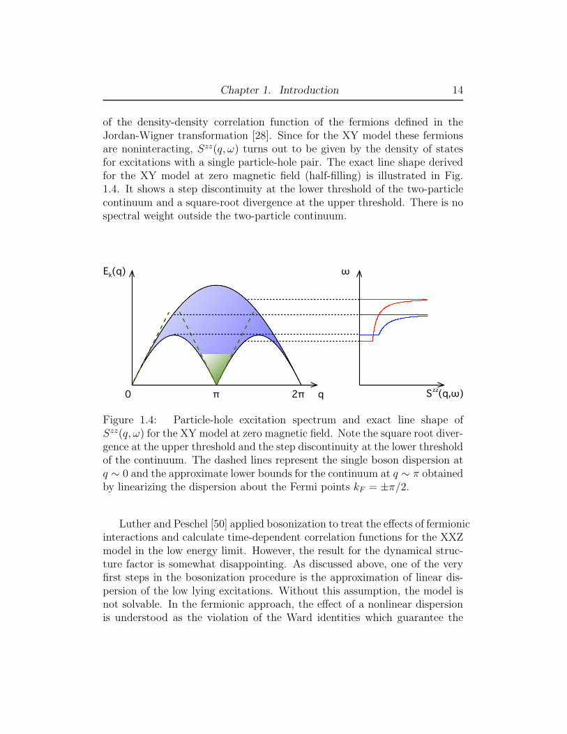
of the density-density correlation function of the fermions defined in theJordan-Wigner transformation [28]. Since for the XY model these fermionsare noninteracting, Szz(q, ω) turns out to be given by the density of statesfor excitations with a single particle-hole pair. The exact line shape derivedfor the XY model at zero magnetic field (half-filling) is illustrated in Fig.1.4. It shows a step discontinuity at the lower threshold of the two-particlecontinuum and a square-root divergence at the upper threshold. There is nospectral weight outside the two-particle continuum.

q

E (q)k

π 2π0 S (q,ω)zz

ω

Figure 1.4: Particle-hole excitation spectrum and exact line shape ofSzz(q, ω) for the XY model at zero magnetic field. Note the square root diver-gence at the upper threshold and the step discontinuity at the lower thresholdof the continuum. The dashed lines represent the single boson dispersion atq ∼ 0 and the approximate lower bounds for the continuum at q ∼ π obtainedby linearizing the dispersion about the Fermi points kF = ±π/2.

Luther and Peschel [50] applied bosonization to treat the effects of fermionicinteractions and calculate time-dependent correlation functions for the XXZmodel in the low energy limit. However, the result for the dynamical struc-ture factor is somewhat disappointing. As discussed above, one of the veryfirst steps in the bosonization procedure is the approximation of linear dis-persion of the low lying excitations. Without this assumption, the model isnot solvable. In the fermionic approach, the effect of a nonlinear dispersionis understood as the violation of the Ward identities which guarantee the


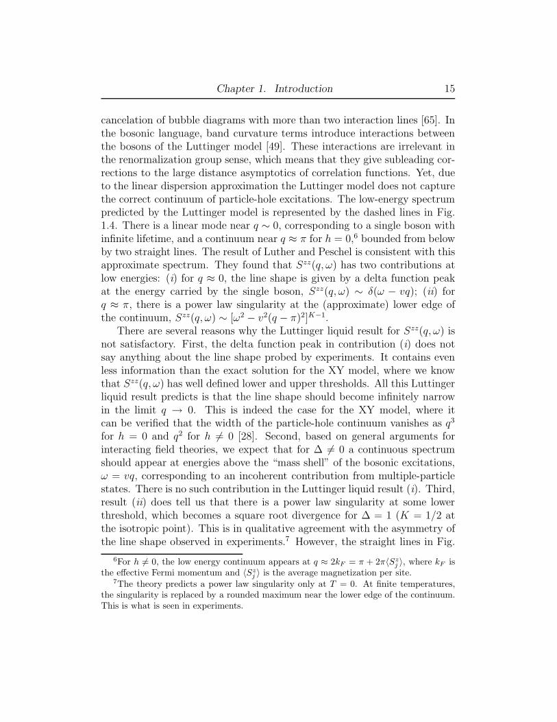
cancelation of bubble diagrams with more than two interaction lines [65]. Inthe bosonic language, band curvature terms introduce interactions betweenthe bosons of the Luttinger model [49]. These interactions are irrelevant inthe renormalization group sense, which means that they give subleading cor-rections to the large distance asymptotics of correlation functions. Yet, dueto the linear dispersion approximation the Luttinger model does not capturethe correct continuum of particle-hole excitations. The low-energy spectrumpredicted by the Luttinger model is represented by the dashed lines in Fig.1.4. There is a linear mode near q ∼ 0, corresponding to a single boson withinfinite lifetime, and a continuum near q ≈ π for h = 0,6 bounded from belowby two straight lines. The result of Luther and Peschel is consistent with thisapproximate spectrum. They found that Szz(q, ω) has two contributions atlow energies: (i) for q ≈ 0, the line shape is given by a delta function peakat the energy carried by the single boson, Szz(q, ω) ∼ δ(ω − vq); (ii) forq ≈ π, there is a power law singularity at the (approximate) lower edge ofthe continuum, Szz(q, ω) ∼ [ω2 − v2(q − π)2]K−1.

There are several reasons why the Luttinger liquid result for Szz(q, ω) isnot satisfactory. First, the delta function peak in contribution (i) does notsay anything about the line shape probed by experiments. It contains evenless information than the exact solution for the XY model, where we knowthat Szz(q, ω) has well defined lower and upper thresholds. All this Luttingerliquid result predicts is that the line shape should become infinitely narrowin the limit q → 0. This is indeed the case for the XY model, where itcan be verified that the width of the particle-hole continuum vanishes as q3

for h = 0 and q2 for h 6= 0 [28]. Second, based on general arguments forinteracting field theories, we expect that for ∆ 6= 0 a continuous spectrumshould appear at energies above the “mass shell” of the bosonic excitations,ω = vq, corresponding to an incoherent contribution from multiple-particlestates. There is no such contribution in the Luttinger liquid result (i). Third,result (ii) does tell us that there is a power law singularity at some lowerthreshold, which becomes a square root divergence for ∆ = 1 (K = 1/2 atthe isotropic point). This is in qualitative agreement with the asymmetry ofthe line shape observed in experiments.7 However, the straight lines in Fig.

6For h 6= 0, the low energy continuum appears at q ≈ 2kF = π + 2π〈Szj 〉, where kF is

the effective Fermi momentum and 〈Szj 〉 is the average magnetization per site.

7The theory predicts a power law singularity only at T = 0. At finite temperatures,the singularity is replaced by a rounded maximum near the lower edge of the continuum.This is what is seen in experiments.


1.4 are not the real edges of the two-particle continuum, except at q = π.There is no guarantee that the Luttinger liquid exponent for the power lawsingularity is the correct one away from q = π. Furthermore, result (ii) doesnot predict the behavior of Szz(q, ω) at higher energies, particularly at theupper threshold of the two-particle continuum, which is beyond the reach ofthis approximation.

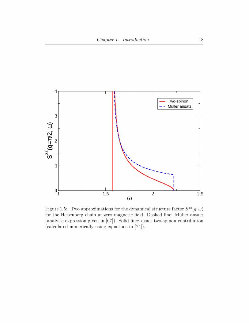
In the lack of a useful field theory result, in 1979 Muller et al. [66] putforward an approximate analytic expression for Szz(q, ω) for the Heisenbergchain. Their proposal (detailed in [67]) was inspired by the exact solutionfor the XY model, selection rules for classes of Bethe ansatz eigenstates,numerical results for short chains (N ≤ 10) as well as known sum rules [68].The formula which became known as the Muller ansatz assumes that almostall the spectral weight is confined within the thresholds of the (later named)two-spinon continuum. The line shape predicted by the Muller ansatz isplotted in Fig. 1.5. Note that, contrary to the result for the XY model,there is a power law divergence at the lower threshold and a step function atthe upper threshold. The square root singularity at the lower threshold waschosen to agree with the field theory result of Luther and Peschel at q ≈ π.As Muller et al. noted themselves, their formula could not be exact, not onlybecause it cannot satisfy all the sum rules simultaneously, but also becauseit does not account for the spectral weight above the upper boundary ofthe two-spinon continuum, which was clearly seen in the numerical results.Nonetheless, the Muller ansatz proved quite useful in analyzing experimentaldata [69]. A generalization of the Muller ansatz for the XXZ chain in thegapless regime was presented in [70].

Later it was shown that the dynamical structure factor for the relatedHaldane-Shastry model (isotropic spin-1/2 chain with long range 1/r2 inter-action) can be calculated exactly [71]. This model is equivalent to a gas ofnoninteracting spinons, therefore only two-spinon excitations contribute toSzz(q, ω). Interestingly, the exact result for Szz(q, ω) of the Haldane-Shastrymodel coincides with the Muller ansatz, although the expressions for thethresholds of the two-spinon continuum are different.

Substantial progress was made in 1996 when Bougourzi et al. [72] appliedquantum group methods developed by Jimbo and Miwa [73] and calculatedthe exact two-spinon contribution to Szz(q, ω) for the Heisenberg model atzero field. Their solution exploits the infinite symmetry of the XXZ chain inthe massive Neel phase directly in the thermodynamic limit. The expressionfor the form factors for the two-spinon states are obtained by taking the


limit ∆ → 1 from above. The two-spinon dynamical structure factor [74] isillustrated in Fig. 1.5. Although more complicated than the Muller ansatz,this result confirms a square root divergence, accompanied by a logarithmiccorrection, at the lower edge of the two-spinon continuum. At the upperedge, however, the two-spinon contribution vanishes in a square-root cusp.Note that this is still not the full solution for the Heisenberg chain, sincefour and higher spinon states also contribute to Szz(q, ω), but there are noanalytic formulas for the corresponding form factors. However, the exact twospinon result by itself is a good approximation because it accounts for 72.89%of the total spectral weight in the integrated intensity [74]. In fact, the two-spinon solution was shown to be in better agreement with experiments thanthe Muller ansatz [14], since the latter overestimates the spectral weight atthe upper boundary of the two-spinon band.

The solution of Bougourzi et al. is not applicable in the gapless regime ofthe XXZ chain. Moreover, there are no such analytical results for the Heisen-berg chain at nonzero magnetic field. However, more recently a method basedon the Algebraic Bethe Ansatz (or Quantum Inverse Scattering Method [19])was developed which allows one to derive determinant expressions for formfactors between Bethe ansatz eigenstates for finite chains [75]. These ex-pressions can be evaluated numerically for fairly large chains (of the orderof a few hundred sites in most cases). By focusing on the dominant classesof eigenstates, the dynamical structure factors can be computed numericallyfor arbitrary values of anisotropy and field [76]. The main drawback of thisapproach are strong finite size effects.

Remarkably, the study of dynamical correlation functions had advancedmore on the Bethe ansatz front than on the field theoretical one, which hadbeen so fruitful in the calculation of thermodynamic properties and equal-time correlations. At the time the research reported here was started, afield theory interpretation of the emergence of a two-particle continuum withedge singularities having the Luttinger model as the starting point was stillmissing.

1.7 Beyond the Luttinger liquid paradigm

The calculation of the dynamical structure factor exposes a limitation of theLuttinger model as the effective field theory for the XXZ spin chain. Thepeak in the line shape of Szz(q, ω) for small q is infinitely sharp because the


1 1.5 2 2.5ω

0

1

2

3

4

Szz

(q=

π/2,

ω)

Two-spinonMuller ansatz

Figure 1.5: Two approximations for the dynamical structure factor Szz(q, ω)for the Heisenberg chain at zero magnetic field. Dashed line: Muller ansatz(analytic expression given in [67]). Solid line: exact two-spinon contribution(calculated numerically using equations in [74]).


Luttinger model is Lorentz invariant, implying that the bosonic excitationspropagate ballistically with velocity v. Lorentz invariance is not a symmetryof the original lattice model; it only emerges in the low-energy limit. Inorder to obtain a peak with finite width, it is necessary to go beyond thefree boson picture and treat irrelevant interactions properly. This turns outto be a nontrivial task, because simple perturbation theory in the irrelevantoperators can lead to infrared divergences [77].

The problem of the finite width of the dynamical structure factor alsoappears in the context of electron transport in quasi-1D wires. The relatedquantity there is the imaginary part of the density-density correlation func-tion. It was pointed out in [78] that, as a consequence of the linear dispersionapproximation, the Luttinger model does not account for the leading contri-bution to the Coulomb drag response between quantum wires with differentelectronic densities. Following an alternative route to bosonization, Pustil-nik et al. [79] studied the dynamical structure factor for spinless fermionswith parabolic dispersion using perturbation theory in the interaction. Thisproblem is analogous to the spin chain at finite magnetic field in the limit∆ ≪ 1. The fermionic approach to calculate Szz(q, ω) treats band curvatureexactly, but faces logarithmic divergences which appear in all orders of per-turbation theory. The divergences can be dealt with by using a formalismdeveloped in the study of X-ray edge singularities in metals [80]. Pustilniket al. found that the most striking effect of interactions on the dynamicalstructure factor is to induce power-law singularities at the thresholds of theparticle-hole continuum. The q-dependent exponents are not clearly relatedto any previously known exponents calculated in Luttinger liquid theory.Interestingly, an extrapolation of the results of Pustilnik et al. to stronginteractions seemed very promising since the asymmetric line shape that re-sults from their approach is reminiscent of the one expected for spin chains.However, the two-spinon result for the Heisenberg point suggests that the ex-ponents should be independent of momentum in the zero field (particle-holesymmetric) case.

The limitations of the Luttinger model are even more critical when itcomes to correlation functions at finite temperature. In general, one expectsthat at finite temperature inelastic scattering will generate a finite decayrate for the quasiparticles of an interacting system. In the Luttinger model,however, the dynamical structure factor for small q remains a delta functionpeak for T > 0. This means that the bosonic modes still propagate ballisti-cally in the scaling limit [57]. The question then is whether this remains true


once we include irrelevant interactions between the bosons. Surprisingly, theanswer seems to depend on high-energy properties such as the integrabilityof the lattice model. One way to probe the propagation of excitations isby means of transport properties. It is now well accepted that the dc heatconductivity calculated using the Kubo formula [81] should be infinite forthe XXZ model because the heat current operator is a nontrivial conservedquantity [82]. Indeed, experiments show that the mean free path for thermaltransport in spin chain compounds is limited by spin defects, rather thanintrinsic scattering between spinons [83].

The problem of spin transport (equivalent to charge transport in thefermionic version) is less clear. The spin current operator does not com-mute with the Hamiltonian, except in the trivial noninteracting case (theXY model). Nonetheless, Zotos et al. [82] have conjectured that the spinDrude weight, defined as the coefficient of the delta function peak in theconductivity at zero frequency, should be finite for integrable models. Afinite Drude weight implies an infinite dc spin conductivity at finite tem-peratures. This means that the existence of nontrivial conserved quantitiesshould protect the ballistic propagation of the excitations. So far it has notbeen possible to address this question using field theory methods because notmuch is known about the role of integrability in low-energy effective models.It has been suggested that, contrary to the conjecture, a finite Drude weightcould be generic to 1D models which have the Luttinger model as fixed point[84]. However, this conclusion cannot be correct because, as pointed out in[85], the presence of certain irrelevant interactions neglected in [84] can makethe Drude weight vanish, rendering the conductivity finite.

Evidence for a diffusive behavior in Heisenberg spin chains has beenclaimed in [86]. By doing oxygen NMR in Sr2CuO3, Thurber et al. were ableto separate the contribution from the low-energy modes with q ≈ 0 to thespin-lattice relaxation rate 1/T1. The Luttinger model predicts that 1/(T1T )is given by a magnetic-field-independent constant at low temperatures. How-ever, the experiment suggested that 1/(T1T ) diverges with decreasing fieldas 1/

√ωn ∝ h−1/2, where ωn is the nuclear magnetic resonance frequency.

This is a signature of diffusive behavior, which is well established in higherdimensions [87]. The frequency dependence of the NMR response is relatedto the long-time decay of short distance spin correlations, in particular theself-correlation function 〈Sz

j (t)Szj (0)〉. In one dimension, diffusive behavior

is equivalent to a 1/√

t decay of the self-correlation function. This is not


the result expected within the Luttinger model, but the long-time behavioris not necessarily determined by low-energy modes. Apparently, spin diffu-sion conflicts with the picture of ballistically propagation bosons which isthe basis of the Luttinger liquid paradigm. It also seems to contradict theconjecture about ideal transport in integrable spin chains. If correct, thisexperimental result could change the way we think about excitations of 1Dmodels. Understanding the behavior of time-dependent correlation functionsat zero temperature constitutes an important step towards answering thesequestions.

1.8 Overview

This thesis is a theoretical study of various aspects of the longitudinal dynam-ical structure factor for the XXZ model at zero temperature. Our goal was toderive analytic formulas for the width, tail and edge singularities of Szz(q, ω)which are nonperturbative in the anisotropy parameter ∆ and therefore holdin the entire critical region of the phase diagram. This could only be ac-complished by combining field theory methods with the exact Bethe ansatzsolution in ways that had not been explored before.

The next chapters are organized as follows. Chapter 2 focuses on thebroadening of the on-shell peak of Szz(q, ω) at finite magnetic field and inthe limit of small q. By treating the leading irrelevant operators which ac-count for band curvature effects, I show that the width of the on-shell peakscales as q2 in the interacting case, similarly to the exact result for the XYmodel. I relate the coefficient of the q2 dependence to a coupling constantof the low-energy effective model which can be calculated using the Betheansatz solution. This provide a formula for the width of Szz(q, ω) at finitefield which is asymptotically exact in the limit of small q. Another impor-tant result in this chapter is that the line shape which arises from addingboson decay processes to the Luttinger model is not a Lorentzian. Withinthe approximation which neglects dimension-four and higher irrelevant op-erators, the peak has a rectangular shape with well-defined lower and upperthresholds. These are identified with the energy thresholds for the creationof particle-hole pair excitations in the Bethe ansatz solution. In Chapter 3, Ishow that the low-energy effective theory with irrelevant operators can alsoaccount for the spectral weight above the upper threshold of the particle-holecontinuum. Besides deriving formulas for the high-frequency tail of Szz(q, ω)


at both zero and finite magnetic field, I show that integrability affects the lineshape of Szz(q, ω) at zero field in a noticeable way. This is because the conser-vation of the energy current operator rules out a boson decay process which,if present in the effective Hamiltonian, would modify the high-frequency tailnear the upper threshold of the two-particle continuum. The question ofwhat happens at the thresholds of the two-particle continuum is addressedin Chapter 4. I apply the afore mentioned analogy with the X-ray edgeproblem and derive an effective Hamiltonian to study the edge singularitiesof Szz(q, ω). The results in this chapter are not restricted to low energiesand small q. The main result there is the derivation of exact formulas for thesingularity exponents in terms of phase shifts which can be extracted fromthe Bethe ansatz equations. This approach reproduces the singularities ofthe two-spinon dynamical structure factor for the Heisenberg chain as a spe-cial case. In addition, I show that the edge singularities govern the long-timebehavior of the self-correlation function. I prove that the leading term in thelong-time asymptotics is not the one given by the Luttinger liquid result, butinvolves high-energy particle-hole excitations near the top and bottom of theband. Finally, in Chapter 5 I make some concluding remarks and suggestionsfor future research.

23

Bibliography

[1] T. Giamarchi, Quantum physics in One Dimension (Clarendon Press,Oxford, 2004).

[2] P. Fazekas, Lecture Notes on Electron Correlation and Magnetism

(World Scientific, Singapore, 1999).

[3] S. C. Benjamin and S. Bose, Phys. Rev. Lett. 90, 247301 (2003).

[4] S. Schaffer-Nameki, J. Stat. Mech. p. N12001 (2006).

[5] W. Heisenberg, Z. Phys. 49, 619 (1928).

[6] P. A. M. Dirac, The Principles of Quantum Mechanics (Oxford Univer-sity Press, London, 1947).

[7] P. W. Anderson, Phys. Rev. 86, 694 (1952).

[8] N. D. Mermin and H. Wagner, Phys. Rev. Lett. 17, 1133 (1966).

[9] P. C. Hohenberg, Phys. Rev. 158, 383 (1967).

[10] S. Coleman, Comm. Math. Phys. 31, 259 (1973).

[11] N. Motoyama, H. Eisaki, and S. Uchida, Phys. Rev. Lett. 76, 3212(1996).

[12] P. W. Anderson, Phys. Rev. 115, 2 (1959).

[13] I. Yamada and H. Onda, Phys. Rev. B 49, 1048 (1994).

[14] M. B. Stone, D. H. Reich, C. Broholm, K. Lefmann, C. Rischel, C. P.Landee, and M. M. Turnbull, Phys. Rev. Lett. 91, 037205 (2003).

[15] H. Bethe, Z. Phys. 71, 205 (1931).

Bibliography 24

[16] B. Sutherland, Beautiful Models (World Scientific, 2004).

[17] E. H. Lieb and W. Liniger, Phys. Rev. 130, 1605 (1963).

[18] E. H. Lieb and F. Y. Wu, Phys. Rev. Lett. 20, 1445 (1968).

[19] V. E. Korepin, N. M. Bogoliubov, and A. G. Izergin, Quantum in-

verse scattering method and correlation functions (Cambridge UniversityPress, 1993).

[20] M. Takahashi, Thermodynamics of one-dimensional solvable problems

(Cambridge University Press, 1999).

[21] J. des Cloizeaux and J. J. Pearson, Phys. Rev. 128, 2131 (1962).

[22] R. Hagemans and J.-S. Caux, J. Phys. A: Math. Theor. 40, 14605 (2007).

[23] L. Hulthen, Arkiv Mat. Astron. Fysik 26A, 1 (1938).

[24] R. B. Griffiths, Phys. Rev. 133, A768 (1964).

[25] F. Woynarovich and H.-P. Eckle, J. Phys. A: Math. Gen. 20, L97 (1987).

[26] J. L. Cardy, J. Phys. A: Math. Gen. 17, L385 (1984).

[27] M. Takahashi, Prog. Theor. Phys. 46, 401 (1971).

[28] E. Lieb, T. Schultz, and D. Mattis, Ann. Phys. (N.Y) 16, 407 (1961).

[29] F. D. M. Haldane, Phys. Lett. 93A, 464 (1983).

[30] I. Affleck, T. Kennedy, E. H. Lieb, and H. Tasaki, Phys. Rev. Lett. 59,799 (1987).

[31] I. Affleck, J. Phys.: Condens. Matter 1, 3047 (1989).

[32] C. N. Yang and C. P. Yang, Phys. Rev. 150, 321 (1966).

[33] R. Orbach, Phys. Rev. 112, 309 (1958).

[34] I. Affleck and M. Oshikawa, Phys. Rev. B 60, 1038 (1999).

[35] B. C. Watson, V. N. Kotov, M. W. Meisel, D. W. Hall, G. E. Granroth,W. T. Montfrooij, S. E. Nagler, D. A. Jensen, R. Backov, M. A. Petruska,et al., Phys. Rev. Lett. 86, 5168 (2001).

Bibliography 25

[36] F. Mila, Eur. Phys. J. B 6, 201 (1998).

[37] K. Totsuka, Phys. Rev. B 57, 3454 (1998).

[38] L. I. Glazman and A. I. Larkin, Phys. Rev. Lett. 79, 3736 (1997).

[39] F. Meier, J. Levy, and D. Loss, Phys. Rev. Lett. 90, 047091 (2003).

[40] L.-M. Duan, E. Demler, and M. D. Lukin, Phys. Rev. Lett. 91, 090402(2003).

[41] T. Kinoshita, T. Wenger, and D. S. Weiss, Nature 440, 900 (2006).

[42] B. M. McCoy, Phys. Rev. 173, 531 (1968).

[43] L. D. Landau, Sov. Phys. JETP 8, 70 (1959).

[44] A. A. Abrikosov, L. P. Gorkov, and I. E. Dzyaloshinski, Methods of

Quantum Field Theory in Statistical Physics (Dover Publications, NewYork, 1975).

[45] J. Voit, Rep. Prog. Phys. 57, 977 (1994).

[46] A. O. Gogolin, A. A. Nersesyan, and A. M. Tsvelik, Bosonization Ap-

proach to Strongly Correlated Systems (Cambridge University Press,1999).

[47] J. M. Luttinger, J. Math. Phys. 4, 1154 (1963).

[48] M. G. K.-V. Pham and P. Lederer, Phys. Rev. B 61, 16397 (2000).

[49] F. D. M. Haldane, J. Phys. C 14, 2585 (1981).

[50] A. Luther and I. Peschel, Phys. Rev. B 12, 3908 (1975).

[51] I. Affleck, J. Phys. A: Math. Gen. 31, 4573 (1998).

[52] P. D. Francesco, P. Mathieu, and D. Senechal, Conformal Field Theory

(Springer-Verlag, New York, 1997).

[53] I. Affleck, Fields, Strings and Critical Phenomena (Les Houches, SessionXLIX, Amsterdam: North-Holland, 1988), p. p. 563, edited by E. Brezinand J. Zinn-Justin.

Bibliography 26

[54] W. M. C. Foulkes, L. Mitas, R. J. Needs, and G. Rajagopal, Rev. Mod.Phys. 73, 33 (2001).

[55] U. Schollwock, Rev. Mod. Phys. 77, 259 (2005).

[56] S. Eggert, I. Affleck, and M. Takahashi, Phys. Rev. Lett. 73, 332 (1994).

[57] S. Sachdev, Phys. Rev. B 50, 13006 (1994).

[58] M. Takigawa, N. Motoyama, H. Eisaki, and S. Uchida, Phys. Rev. Lett.76, 4612 (1996).

[59] M. Oshikawa and I. Affleck, Phys. Rev. Lett. 82, 5136 (1999).

[60] S. M. Lovesey, Theory of Thermal Neutron Scattering from Condensed

Matter (Clarendon Press, Oxford, 1984).

[61] Y. Endoh, G. Shirane, R. J. Birgeneau, P. M. Richards, and S. L. Holt,Phys. Rev. Lett. 32, 170 (1973).

[62] I. U. Heilmann, G. Shirane, Y. Endoh, R. J. Birgeneau, and S. L. Holt,Phys. Rev. B 18, 3530 (1978).

[63] T. Todani and K. Kawasaki, Prog. Theor. Phys. Jpn. 50, 1216 (1973).

[64] H. J. Mikeska, Phys. Rev. B 12, 2794 (1975).

[65] J. Solyom, Adv. Phys. 28, 201 (1979).

[66] G. Muller, H. Beck, and J. C. Bonner, Phys. Rev. Lett. 43, 75 (1979).

[67] G. Muller, H. Thomas, H. Beck, and J. C. Bonner, Phys. Rev. B 24,1429 (1981).

[68] P. C. Hohenberg and W. F. Brinkman, Phys. Rev. B 10, 128 (1952).

[69] S. E. Nagler, D. A. Tennant, R. A. Coweley, T. G. Perring, and S. K.Satija, Phys. Rev. B 44, 12361 (1991).

[70] G. Muller, H. Thomas, M. Puggat, and H. Beck, J. Phys. C: Solid StatePhys. 14, 3399 (1981).

[71] F. D. M. Haldane and M. R. Zirnbauer, Phys. Rev. Lett. 71, 4055 (1993).

Bibliography 27

[72] A. H. Bougourzi, M. Couture, and M. Kacir, Phys. Rev. B 54, R12669(1996).

[73] M. Jimbo and T. Miwa, Algebraic analysis of Solvable Lattice Models

(Providence, RI: AMS, 1995).

[74] M. Karbach, G. Muller, A. H. Bougourzi, A. Fledderjohann, and K.-H.Mutter, Phys. Rev. B 55, 12510 (1997).

[75] N. Kitanine, J. M. Maillet, and V. Terras, Nucl. Phys. B 554, 647 (1999).

[76] J.-S. Caux and J. M. Maillet, Phys. Rev. Lett. 95, 077201 (2005).

[77] K. Samokhin, J. Phys.: Cond. Mat. 10, L533 (1998).

[78] M. Pustilnik, E. G. Mishchenko, L. I. Glazman, and A. V. Andreev,Phys. Rev. Lett. 91, 126805 (2003).

[79] M. Pustilnik, M. Khodas, A. Kamenev, and L. I. Glazman, Phys. Rev.Lett. 96, 196405 (2006).

[80] K. D. Schotte and U. Schotte, Phys. Rev. 182, 479 (1969).

[81] G. D. Mahan, Many-Particle Physics (Kluwer/Plenum, New York,2000), 3rd ed.

[82] X. Zotos, F. Naef, and P. Prelovsek, Phys. Rev. B 55, 11029 (1997).

[83] T. Kawamata, N. Takahashi, T. Adachi, T. Noji, K. Kudo,N. Kobayashi, and Y. Koike, arXiv:0803.2400 (2008).

[84] S. Fujimoto and N. Kawakami, Phys. Rev. Lett. 90, 197202 (2003).

[85] A. Rosch and N. Andrei, Phys. Rev. Lett. 85, 1092 (2000).

[86] K. R. Thurber, A. W. Hunt, T. Imai, and F. C. Chou, Phys. Rev. Lett.87, 247202 (2001).

[87] P. G. de Gennes, J. Phys. Chem. Solids 4, 223 (1958).

28

Chapter 2

Broadening of the dynamical

structure factor by boson decay

This chapter name is very long and does not display properly in the runningheaders or in the table of contents. To deal with this, we provide a shorterversion of the title as the optional argument to the \chapter[]{} command.

For example, this chapter’s title and associated table of contents headingand running header was created with\chapter[Another Chapter\ldots]{Another Chapter with a Very Long

Chapter-name that will Probably Cause Problems}.Note that, according to the thesis regulations, the heading included in

the table of contents must be a truncation of the actual heading.

2.1 Another Section

Another bunch of text to demonstrate what this file does. You might wanta list for example:1

• An item in a list.

• Another item in a list.

1Here is a footnote in a different chapter. Footnotes should come after punctuation.

29

Chapter 3

High-frequency tail

30

Chapter 4

Edge singularities and

long-time decay

31

Additional Information

This chapter shows you how to include additional information in your thesis,the removal of which will not affect the submission. Such material should beremoved before the thesis is actually submitted.

First, the chapter is unnumbered and not included in the Table of Con-tents. Second, it is the last section of the thesis, so its removal will not alterany of the page numbering etc. for the previous sections. Do not include anyfloats, however, as these will appear in the initial lists.

The ubcthesis LATEX class has been designed to aid you in produc-ing a thesis that conforms to the requirements of The University of BritishColumbia Faculty of Graduate Studies (FoGS).

Proper use of this class and sample is highly recommended—and shouldproduce a well formatted document that meets the FoGS requirement. Notwith-standing, complex theses may require additional formatting that may con-flict with some of the requirements. We therefore highly recommend that youconsult one of the FoGS staff for assistance and an assessment of potentialproblems before starting final draft.

While we have attemped to address most of the thesis formatting require-ments in these files, they do not constitute an official set of thesis require-ments. The official requirements are available at the following section of theFoGS web site:

http://www.grad.ubc.ca/students/thesis/

We recommend that you review these instructions carefully.

Documents

Dynamical correlations of S = 1 2 quantum spin chainsiaffleck/per-the.pdf · Dynamical correlations of S = 1/2 quantum ... acting spins that behave according to the rules of quantum