Embed Size (px)
Citation preview
Dynamic Spectral Clustering based onKernels
Diego Hernan Peluffo Ordonez
National University of Colombia - ManizalesFaculty of Engineering and Architecture
Department of Electric Engineering, Electronics and Computing ScienceManizales, Colombia
2013

Dynamic Spectral Clustering based onKernels
Diego Hernan Peluffo Ordonez
Thesis presented as a partial request for the degree of:Doctor of Engineering - Automatics
Director:Ph.D. Cesar German Castellanos Domınguez
Research subject:Spectral Clustering and Dynamic Data Analysis
Research Group:Digital Signal Processing and Recognition Group
National University of Colombia - ManizalesFaculty of Engineering and Architecture
Department of Electric Engineering, Electronics and Computing ScienceManizales, Colombia
2013


Agrupamiento espectral de datosdinamicos
Diego Hernan Peluffo Ordonez
Esta tesis se presenta como requisito parcial para optar al tıtulo de :Doctor en Ingerıa - Lınea de Automatica
Director:Prof. Cesar German Castellanos Domınguez
Tema de investigacion:Agrupamiento espectral y analisis de datos dinamicos
Grupo de investigacion:Grupo de control y procesamiento digital de senales
Universidad Nacional de Colombia, sede ManizalesFacultad de Ingenierıa y Arquitectura
Departamento de Ingenierıa Electrica, Electronica y SistemasManizales, Colombia
2013


To my parents
A mis padres


Acknowledgements
First, I would like to express my sincere gratitude to Prof. German Castellanos, who wasthe advisor to develop this work. I thank him for the continuous support of my study andresearch training, as well as for his motivation and immense knowledge. Undoubtedly, hisguidance was a major factor to achieve this goal in terms of both research and writing of thisthesis.
Also, I want to thank the members of my thesis committee: Prof. Johan Suykens, PhD.Carlos Alzate, Prof. Claudia Isaza, Prof. Jose Luis Rodrıguez, and Prof. Mauricio Orozco.To all of them, thanks for their encouragement, insightful comments, revisions and construc-tive questions. Especially, my sincere thanks goes to Prof. Johan Suykens and PhD. CarlosAlzate for offering me the chance for an internship in their research group and guiding meworking on suitable and interesting topics to deal with this thesis’ issues.
Now I would like to post my thanks to all my fellow research group. Especially, I thankto Sergio Garcıa, Cristian Castro, Santiago Murillo, and Andres Castro for the helpful dis-cussions, and support. I thank to them not only for academic matters but also for theirfriendship which encouraged me to finish this process. My heartfelt thanks goes for mygreat friend Yenny Berrıo. She always found a way to encourage me in hard moments, de-spite the circumstances, with kindness and support. Thanks also to all the people (teachersand friends) who helped me somehow with the writing review. Another special thanks goesto Julie (Yoly kitty) who is such as an angel to me. She encourages me in both personal andspiritual matters. Also, she helped a lot checking the manuscript writing.
I thank my family: my parents Mario Peluffo and Guilnar Ordonez, and my brother MarioEduardo Peluffo, for supporting me spiritually throughout the course of this work and mywhole life.
Last but not the least, I thank God to provide me life, wisdom and strength to finish success-fully this stage of my life.


This work was supported by the research project “Grupo de control yprocesamiento digital de senales” identified with code 20501007205.

Abstract
The analysis of dynamic or time-varying data has emerged as an issue of great interest tak-ing increasingly an important place in scientific community, especially in automation, pat-tern recognition and machine learning. There exists a broad range of important applicationssuch as video analysis, motion identification, segmentation of human motion and airplanetracking, among others. Spectral matrix analysis is one of the approaches to address thisissue. Spectral techniques, mainly those based on kernels, have proved to be a suitable toolin several aspects of interest in pattern recognition and machine learning even when dataare time-varying, such as the estimation of the number of clusters, clustering and classifica-tion. Most of spectral clustering approaches have been designed for analyzing static data,discarding the temporal information, i.e. the evolutionary behavior along time. Some workshave been developed to deal with the time varying effect. Nonetheless, an approach ableto accurately track and cluster time-varying data in real time applications remains an openissue.
This thesis describes the design of a kernel-based dynamic spectral clustering using a primal-dual approach so as to carry out the grouping task involving the dynamic information, thatis to say, the changes of data frames along time. To this end, a dynamic kernel frameworkaimed to extend a clustering primal formulation to dynamic data analysis is introduced. Suchframework is founded on a multiple kernel learning (MKL) approach. Proposed clusteringapproach, named dynamic kernel spectral clustering (DKSC) uses a linear combination ofkernels matrices as a MKL model. Kernel matrices are computed from an input frame se-quence represented by data matrices. Then, a cumulative kernel is obtained, being the modelcoefficients or weighting factors obtained by ranking each sample contained in the frame.Such ranking corresponds to a novel tracking approach that takes advantages of the spectraldecomposition of a generalized kernel matrix. Finally, to get the resultant cluster assign-ments, data are clustered using the cumulative kernel matrix.
Experiments are done over real databases (human motion and moon covered by clouds)as well as artificial data (moving-Gaussian clouds). As a main result, proposed spectralclustering method for dynamic data proved to be able for grouping underlying events andmovements and detecting hidden objects as well.
The proposed approach may represent a contribution to the pattern recognition field, mainly,for solving problems involving dynamic information aimed to either tracking or clusteringof data.

14
Keywords
Dynamic or time-varying data, kernels, primal-dual formulation, spectral clustering, supportvector machines
Resumen
El analisis de datos dinamicos o variantes en el tiempo es un tema de gran interes actualpara la comunidad cientıfica, especialmente, en los campos de reconocimiento de patrones yaprendizaje de maquina. Existe un amplio espectro de aplicaciones en donde el analisis dedatos dinamicos toma lugar, tales como el analisis de vıdeo, la identificacion de movimiento,la segmentacion de movimientos de personas y el eguimiento de naves aereas, entre otras.Una de las alternativas para desarrollar metodos dinamicos es el analisis matricial espectral.Las tecnicas espectrales, principalmente aquellas basadas enkernels, han demostrado su altaaplicabilidad en diversos aspectos del reconocimiento de patrones y aprendizaje de maquina,incluso cuando los datos son variantes en el tiempo, tales como la estimacion del numerode grupos, agrupamiento y clasificacion. La mayorıa de los metodos espectrales han sidodisenados para el analisis de datos estaticos, descartando la informacion temporal, es decir,omitiendo el comportamiento y la evolucion de los datos a lo largo del tiempo. En el estadodel arte se encuentran algunos trabajos que consideran el efecto de la variacion en el tiempo,sin embargo, el diseno de un metodo que permita seguir la dinamica de los datos y agruparlos mismos en ambientes de tiempo real, con alta fidelidad y precision, es aun un problemaabierto.
En este trabajo de tesis se presenta un metodo de agrupamiento espectral basado enkernelsdisenado a partir de un enfoque primal-dual con el fin de realizar el proceso de agrupamientoconsiderando la informacion dinamica, es decir, los cambios de secuencia de los datos a lolargo del tiempo. Para este proposito, se plantea un esquema de agrupamiento que consisteen la extension de una formulacion primal-dual al analisis de datos dinamicos a traves deun kerneldinamico. El esquema se basa en un aprendizaje de multipleskernels(MKL) y sedenominadynamic kernel spectral clustering (DKSC). El metodo DKSC usa como modelode MKL una combinacion lineal de matriceskernel. Las matriceskernelse calculan a partirde una secuencia de datos representada por un conjunto de matrices de datos. Subsecuente-mente, se obtiene una matriz acumulada de kernel de tal forma que los coeficientes o factoresde ponderacion del modelo son considerados como valores de evaluacion de cada muestradel conjunto de datos oframe. Dicha evaluacion se hace a partir de un novedoso metodode trackingque se basa en la descomposicion espectral de una matriz kernel generalizada.Finalmente, para la obtencion de las asignaciones de grupo resultantes, los datos son agru-pados usando la matriz acumulada como matriz kernel.

16
Para efectos de experimentacion, se consideran bases de datos reales (movimiento de hu-manos y la luna cubierta por nubes en movimiento) ası como artificiales (nubes Gaussianasen movimiento). Como resultado principal, el metodo propuesto comprobo ser una buenaalternativa para agrupar eventos y movimientos subyacentes ası como para detectar objetosocultos en ambientes cambiantes en el tiempo.Este trabajo puede representar un significativo aporte en el area de reconocimiento de pa-trones, principalmente, en la solucion de problemas que implican datos dinamicos relaciona-dos contrackingo agrupamiento de datos.
Palabras clave
Agrupamiento espectral, datos dinamicos o variantes en el tiempo, formulacion primal-dual,kernels, maquinas de vectores de soporte.

Contents
Acknowledgements 9
Abstract 13
Resumen 15
Contents 20
List of figures 22
List of tables 23
List of algorithms 24
Nomenclature 25
I. Preliminaries 1
1. Introduction 21.1. Motivation and problem statement . . . . . . . . . . . . . . . . . . . .. . 31.2. Objectives . . . . . . . . . . . . . . . . . . . . . . . . . . . . . . . . . . . 4
1.2.1. General objective . . . . . . . . . . . . . . . . . . . . . . . . . . . 41.2.2. Specific Objectives . . . . . . . . . . . . . . . . . . . . . . . . . . 4
1.3. Contributions of this thesis . . . . . . . . . . . . . . . . . . . . . . . .. . 41.4. Manuscript organization . . . . . . . . . . . . . . . . . . . . . . . . . . . 5
2. State of the art on spectral clustering and dynamic data anal ysis 72.1. Spectral clustering . . . . . . . . . . . . . . . . . . . . . . . . . . . . . . 72.2. Kernel-based clustering . . . . . . . . . . . . . . . . . . . . . . . . . .. . 92.3. Dynamic clustering . . . . . . . . . . . . . . . . . . . . . . . . . . . . . .11
18 Contents
II. Methods 12
3. Normalized cut clustering 133.1. Introduction . . . . . . . . . . . . . . . . . . . . . . . . . . . . . . . . . .133.2. Basics of graphs . . . . . . . . . . . . . . . . . . . . . . . . . . . . . . . .13
3.2.1. Graph . . . . . . . . . . . . . . . . . . . . . . . . . . . . . . . . .143.2.2. Weighted graphs . . . . . . . . . . . . . . . . . . . . . . . . . . .143.2.3. Properties and measures . . . . . . . . . . . . . . . . . . . . . . .14
3.3. Clustering Method . . . . . . . . . . . . . . . . . . . . . . . . . . . . . .153.3.1. Multi-cluster partitioning criterion . . . . . . . . . . . . .. . . . . 163.3.2. Matrix representation . . . . . . . . . . . . . . . . . . . . . . . . .163.3.3. Clustering algorithm . . . . . . . . . . . . . . . . . . . . . . . . .17
3.4. Proposed alternatives to solve the NCC problem without using eigenvectors 233.4.1. Heuristic search-based approach . . . . . . . . . . . . . . . . . .. 233.4.2. Quadratic formulation . . . . . . . . . . . . . . . . . . . . . . . .27
4. Kernel spectral clustering 314.1. Introduction . . . . . . . . . . . . . . . . . . . . . . . . . . . . . . . . . .314.2. Kernels for clustering . . . . . . . . . . . . . . . . . . . . . . . . . . . . .32
4.2.1. Kernel function . . . . . . . . . . . . . . . . . . . . . . . . . . . .334.2.2. Types of kernel functions . . . . . . . . . . . . . . . . . . . . . . .34
4.3. Least-squares SVM formulation for kernel spectral clustering . . . . . . . . 364.3.1. Solving the KSC problem . . . . . . . . . . . . . . . . . . . . . .374.3.2. Out-of-sample extension . . . . . . . . . . . . . . . . . . . . . . .394.3.3. KSC algorithm . . . . . . . . . . . . . . . . . . . . . . . . . . . .39
4.4. Proposed data projection for KSC . . . . . . . . . . . . . . . . . . . . .. 394.4.1. Out-of-sample extension of PKSC . . . . . . . . . . . . . . . . . .424.4.2. Estimation of the lower dimension . . . . . . . . . . . . . . . . . .424.4.3. PKSC algorithm . . . . . . . . . . . . . . . . . . . . . . . . . . .43
5. Proposed dynamic spectral clustering 445.1. Introduction . . . . . . . . . . . . . . . . . . . . . . . . . . . . . . . . . .445.2. Multiple kernel learning for clustering . . . . . . . . . . . . . .. . . . . . 455.3. Tracking by KSC . . . . . . . . . . . . . . . . . . . . . . . . . . . . . . .46
5.3.1. Tracking vector . . . . . . . . . . . . . . . . . . . . . . . . . . . .475.3.2. KSC-based tracking algorithm . . . . . . . . . . . . . . . . . . . .525.3.3. Toy example: moving-curve . . . . . . . . . . . . . . . . . . . . .535.3.4. Links with relevance analysis . . . . . . . . . . . . . . . . . . . .57
5.4. Dynamic KSC . . . . . . . . . . . . . . . . . . . . . . . . . . . . . . . . .575.4.1. Dynamic KSC algorithm . . . . . . . . . . . . . . . . . . . . . . .58

Contents 19
III. Experiments and results 59
6. Experimental setup 606.1. Considered database for experiments . . . . . . . . . . . . . . . . .. . . . 60
6.1.1. Real databases . . . . . . . . . . . . . . . . . . . . . . . . . . . .60
6.1.2. Toy databases . . . . . . . . . . . . . . . . . . . . . . . . . . . . .62
6.1.3. Image database . . . . . . . . . . . . . . . . . . . . . . . . . . . .64
6.1.4. Video databases . . . . . . . . . . . . . . . . . . . . . . . . . . . .64
6.2. Clustering Performance Measures . . . . . . . . . . . . . . . . . . . .. . 65
6.2.1. Supervised measures . . . . . . . . . . . . . . . . . . . . . . . . .65
6.2.2. Unsupervised measures . . . . . . . . . . . . . . . . . . . . . . . .68
6.2.3. Proposed performance measures . . . . . . . . . . . . . . . . . . .69
6.3. Experiment description . . . . . . . . . . . . . . . . . . . . . . . . . . . .72
6.3.1. Experiments for assessing the projected KSC performance . . . . . 72
6.3.2. Experiments for KSC-based tracking . . . . . . . . . . . . . . . .72
6.3.3. Experiments for Dynamic KSC . . . . . . . . . . . . . . . . . . .74
7. Results and discussion 777.1. Results for experiments of projected KSC (PKSC) . . . . . . . .. . . . . . 77
7.1.1. Clustering Results of Three-Gaussian Data Sets . . . . . .. . . . . 77
7.1.2. Clustering Results on Artificial Data Sets . . . . . . . . . . .. . . 79
7.1.3. Clustering Results of Real Data . . . . . . . . . . . . . . . . . . .81
7.2. Experimental results for DKSC based on MKL . . . . . . . . . . . . .. . 84
7.2.1. Results for KSC tracking . . . . . . . . . . . . . . . . . . . . . . .84
7.2.2. Results for Three-moving Gaussian database . . . . . . . . .. . . 86
7.2.3. Results for DKSC . . . . . . . . . . . . . . . . . . . . . . . . . .87
7.3. Results for proposed alternatives to NCC . . . . . . . . . . . . . .. . . . . 95
7.3.1. Experimental results for NCChs . . . . . . . . . . . . . . . . . . .95
7.3.2. Experimental results for NCC quadratic formulation . .. . . . . . 99
IV. Final remarks 102
8. Conclusions and future work 1038.1. Conclusions . . . . . . . . . . . . . . . . . . . . . . . . . . . . . . . . . .103
8.2. Future work . . . . . . . . . . . . . . . . . . . . . . . . . . . . . . . . . .104
8.3. Another important remarks . . . . . . . . . . . . . . . . . . . . . . . . . .105

20 Contents
V. Appendixes 106
A. Kernel K-means 107
B. Links with normalized cut clustering 108B.1. Multi-cluster spectral clustering (MCSC) from two pointof view . . . . . . 108B.2. Solving the problem by a difference: Empirical feature map . . . . . . . . . 109
B.2.1. Gaussian processes . . . . . . . . . . . . . . . . . . . . . . . . . .110B.2.2. Eigen-solution . . . . . . . . . . . . . . . . . . . . . . . . . . . .110
C. Links between KSC with normalized cut clustering 111C.1. Multi-cluster spectral clustering (MCSC) from two pointof view . . . . . . 111C.2. Solving the problem by a difference: Empirical feature map . . . . . . . . . 112
C.2.1. Gaussian processes . . . . . . . . . . . . . . . . . . . . . . . . . .113C.2.2. Eigen-solution . . . . . . . . . . . . . . . . . . . . . . . . . . . .113
D. Relevance Analysis for feature extraction and selection vi a spectral anal-ysis 114D.1. Feature relevance . . . . . . . . . . . . . . . . . . . . . . . . . . . . . . .115D.2. Generalized case . . . . . . . . . . . . . . . . . . . . . . . . . . . . . . .116D.3. MSE-based Approach . . . . . . . . . . . . . . . . . . . . . . . . . . . . .117D.4. Q− α Method . . . . . . . . . . . . . . . . . . . . . . . . . . . . . . . . .118D.5. Results . . . . . . . . . . . . . . . . . . . . . . . . . . . . . . . . . . . . .119
E. Academic discussion 126
Bibliography 129

List of Figures
3.1. Weighted graph with three nodes . . . . . . . . . . . . . . . . . . . . . . .14
3.2. Descriptive diagram of spectral clustering algorithm . .. . . . . . . . . . . 17
3.3. Heuristic search and graph . . . . . . . . . . . . . . . . . . . . . . . . . .27
4.1. Feature space to high dimension . . . . . . . . . . . . . . . . . . . . . .. 32
4.2. High dimensional mapping . . . . . . . . . . . . . . . . . . . . . . . . . .34
4.3. Accumulated variance criterion to determine the low dimension . . . . . . 42
5.1. Example of Dynamic Data . . . . . . . . . . . . . . . . . . . . . . . . . .45
5.2. Graphic explanation of MKL for clustering considering the example of chang-ing moon . . . . . . . . . . . . . . . . . . . . . . . . . . . . . . . . . . . 46
5.3. 2-D moving-curve . . . . . . . . . . . . . . . . . . . . . . . . . . . . . . .53
5.4. Clustering of 2-D moving-curve intoK = 3 clusters withNf = 100 framesandN = 100 samples per frame . . . . . . . . . . . . . . . . . . . . . . .55
5.5. Clustering of 2-D moving-curve intoK = 4 clusters withNf = 100 framesandN = 100 samples per frame . . . . . . . . . . . . . . . . . . . . . . .56
6.1. Examples of real data . . . . . . . . . . . . . . . . . . . . . . . . . . . . .61
6.2. Motion Caption Database . . . . . . . . . . . . . . . . . . . . . . . . . . .61
6.3. Subject #1of Motion Caption Database . . . . . . . . . . . . . . . . . . .62
6.4. 2D artificial databases . . . . . . . . . . . . . . . . . . . . . . . . . . . . .62
6.5. Employed 3D databases. . . . . . . . . . . . . . . . . . . . . . . . . . . . . . 63
6.6. Three Gaussian Database . . . . . . . . . . . . . . . . . . . . . . . . . . .63
6.7. Employed images . . . . . . . . . . . . . . . . . . . . . . . . . . . . . . .64
6.8. Moon database . . . . . . . . . . . . . . . . . . . . . . . . . . . . . . . .64
6.9. Example for explanation ofPPQ measure considering three clusters andthree classes . . . . . . . . . . . . . . . . . . . . . . . . . . . . . . . . . .70
6.10. Motion Caption Database . . . . . . . . . . . . . . . . . . . . . . . . . . .73
6.11. Three Gaussian Database . . . . . . . . . . . . . . . . . . . . . . . . . . .73
6.12.Subject #1of Motion Caption Database . . . . . . . . . . . . . . . . . . .75
6.13. Three-moving Gaussian clouds . . . . . . . . . . . . . . . . . . . . . .. . 75

22 List of Figures
7.1. Scatter plots for three-Gaussian data set withµ = [−0.3, 0, 0.3] ands =
[0.1, 0.2, 0.3] (right column), andµ = [−1.8, 0, 1.8] ands = [0.1, 0.2, 0.3](left column) . . . . . . . . . . . . . . . . . . . . . . . . . . . . . . . . . 78
7.2. Clustering performance for three-Gaussian data set withµ = [−1.8, 0, 1.8]ands = (0.1, 0.2, 0.3) . . . . . . . . . . . . . . . . . . . . . . . . . . . . . 79
7.3. HappyFace scatter plots for all studied methods for both training (left col-umn) and test (right column) . . . . . . . . . . . . . . . . . . . . . . . . .80
7.4. IRIS scatter plots for all studied methods for both training (left column) andtest (right column) . . . . . . . . . . . . . . . . . . . . . . . . . . . . . . .81
7.5. Dynamic analysis ofSubject # 2by KSC . . . . . . . . . . . . . . . . . . . 847.6. Clustering results forSubject # 2 . . . . . . . . . . . . . . . . . . . . . . . 857.7. Subject #2tracking . . . . . . . . . . . . . . . . . . . . . . . . . . . . . . 867.8. Tracking Vectors for three-Gaussian moving . . . . . . . . . . .. . . . . . 877.9. Three-moving Gaussian regarding tracking-generated reference labels . . . 887.10. MKL weighting factors forSubject #1 . . . . . . . . . . . . . . . . . . . . 897.11. Clustering results forSubject #1 . . . . . . . . . . . . . . . . . . . . . . . 907.12. Clustering performance for three-moving Gaussian clouds . . . . . . . . . 937.13. Results over moon data set . . . . . . . . . . . . . . . . . . . . . . . . . .947.14. Scatter plots forbullseye andhappyface using the considered cluster-
ing methods . . . . . . . . . . . . . . . . . . . . . . . . . . . . . . . . . .967.15. Clustering performance on image segmentation . . . . . . . .. . . . . . . 987.16. Clustering results after testing of considered databases . . . . . . . . . . . 1007.17. Box plots of time employed for clustering methods. Improved MCSC at left
hand and classical MCSC at right hand . . . . . . . . . . . . . . . . . . . .1007.18. Error bar comparingεM with the number of groups . . . . . . . . . . . . .101
A.1. Graphically explanation of Kernel K-means for pixel clustering oriented toimage segmentation . . . . . . . . . . . . . . . . . . . . . . . . . . . . . .107
D.1. Relevance values for ‘E.coli’ data set. . . . . . . . . . . . . . . .. . . . . 121D.2. Three first principal components of E.coli data set, applying each weighting
method. . . . . . . . . . . . . . . . . . . . . . . . . . . . . . . . . . . . .121D.3. Classification percentage achieved with each weighting method performing
feature extraction (applying PCA). A)No Weighting. B)PCA pre-normalization.C) Eigenvalues weighting. D)Q− α method. E)Q− α method. F)ρ method.G)ρ method. . . . . . . . . . . . . . . . . . . . . . . . . . . . . . . . . . .121
D.4. Classification percentage achieved with each weighting method performingfeature selection. A)No Weighting. B)PCA pre-normalization. C)Q − αmethod. D)Q− α method. E)ρ method. F)ρ method. . . . . . . . . . . . . 122

List of Tables
4.1. Kernel functions . . . . . . . . . . . . . . . . . . . . . . . . . . . . . . . .35
5.1. Notation for the statement of theorems5.3.1and5.3.2. . . . . . . . . . . . 49
6.1. Real Data bases . . . . . . . . . . . . . . . . . . . . . . . . . . . . . . . .606.2. contingency table for comparing two partitions . . . . . . . .. . . . . . . 67
7.1. Overall results for considered real data . . . . . . . . . . . . . .. . . . . . 837.2. Clustering performance forSubject # 2in terms of considered metrics . . . 867.3. Effect of number of groups over theSubject #2 . . . . . . . . . . . . . . . 877.4. NMI and ARI forSubject # 1clustering performance . . . . . . . . . . . . 897.5. Clustering performance per frame for three-moving Gaussian clouds database917.6. Clusterings performance withPPQ along 10 iterations . . . . . . . . . . . 927.7. Mean and standard deviation per cluster . . . . . . . . . . . . . . .. . . . 927.8. Overall results for considered real and toy data along 10 iterations . . . . . 967.9. Clustering performance withPPQ along 10 iterations . . . . . . . . . . . . 977.10. Clustering processing time ratio along 10 iterations . .. . . . . . . . . . . 987.11. Results for toy data sets . . . . . . . . . . . . . . . . . . . . . . . . . . .. 99
D.1. Notation used throughout this chapter . . . . . . . . . . . . . . . .. . . . 114D.2. Classification performance applying feature extraction. Time correspond to
the time needed to calculate the weighting vector, R% is the dimensionalityreduction being 100% the original data set . . . . . . . . . . . . . . . . . .124
D.3. Classification performance applying feature selection.. . . . . . . . . . . . 125
List of Algorithms
1. Normalized cut clustering . . . . . . . . . . . . . . . . . . . . . . . . . . .222. Heuristic Search for Clustering with prior knowledge and pre-clustering . . 28
3. Kernel spectral clustering: [qtrain, qtest] = KSC(X ,K(·, ·),K) . . . . . . . . 394. Projected KSC: [ ˆqtrain, qtest] = PKSC(X ,K(·, ·),K, p) . . . . . . . . . . . . 43
5. KSCT:η = KSCT(X (1), . . . ,X (Nf ), K
). . . . . . . . . . . . . . . . . . . 53
6. DKSC:q
(t)train
Nf
t=1= DKSC
(X (1), . . . ,X (Nf ),K(·, ·),K
). . . . . . . . . . . 58
7. Q− α-based relevance analysis . . . . . . . . . . . . . . . . . . . . . . . .119
Nomenclature
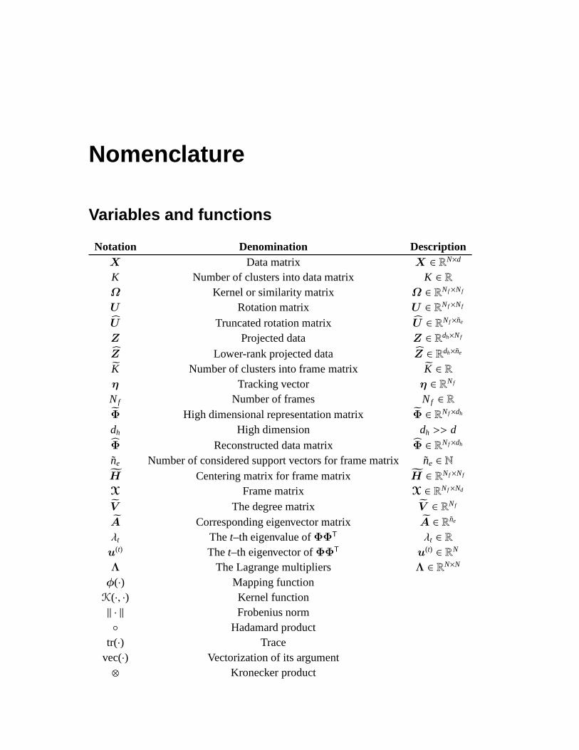
Variables and functions
Notation Denomination DescriptionX Data matrix X ∈ RN×d
K Number of clusters into data matrix K ∈ RΩ Kernel or similarity matrix Ω ∈ RNf×Nf
U Rotation matrix U ∈ RNf×Nf
U Truncated rotation matrix U ∈ RNf×ne
Z Projected data Z ∈ Rdh×Nf
Z Lower-rank projected data Z ∈ Rdh×ne
K Number of clusters into frame matrix K ∈ Rη Tracking vector η ∈ RNf
Nf Number of frames Nf ∈ RΦ High dimensional representation matrix Φ ∈ RNf×dh
dh High dimension dh >> d
Φ Reconstructed data matrix Φ ∈ RNf×dh
ne Number of considered support vectors for frame matrix ˜ne ∈ NH Centering matrix for frame matrix H ∈ RNf×Nf
X Frame matrix X ∈ RNf×Nd
V The degree matrix V ∈ RNf
A Corresponding eigenvector matrix A ∈ Rne
λt Thet–th eigenvalue ofΦΦT λt ∈ R
u(t) Thet–th eigenvector ofΦΦT u(t) ∈ RN
Λ The Lagrange multipliers Λ ∈ RN×N
φ(·) Mapping functionK(·, ·) Kernel function‖ · ‖ Frobenius norm Hadamard product
tr(·) Tracevec(·) Vectorization of its argument⊗ Kronecker product
26 List of Algorithms
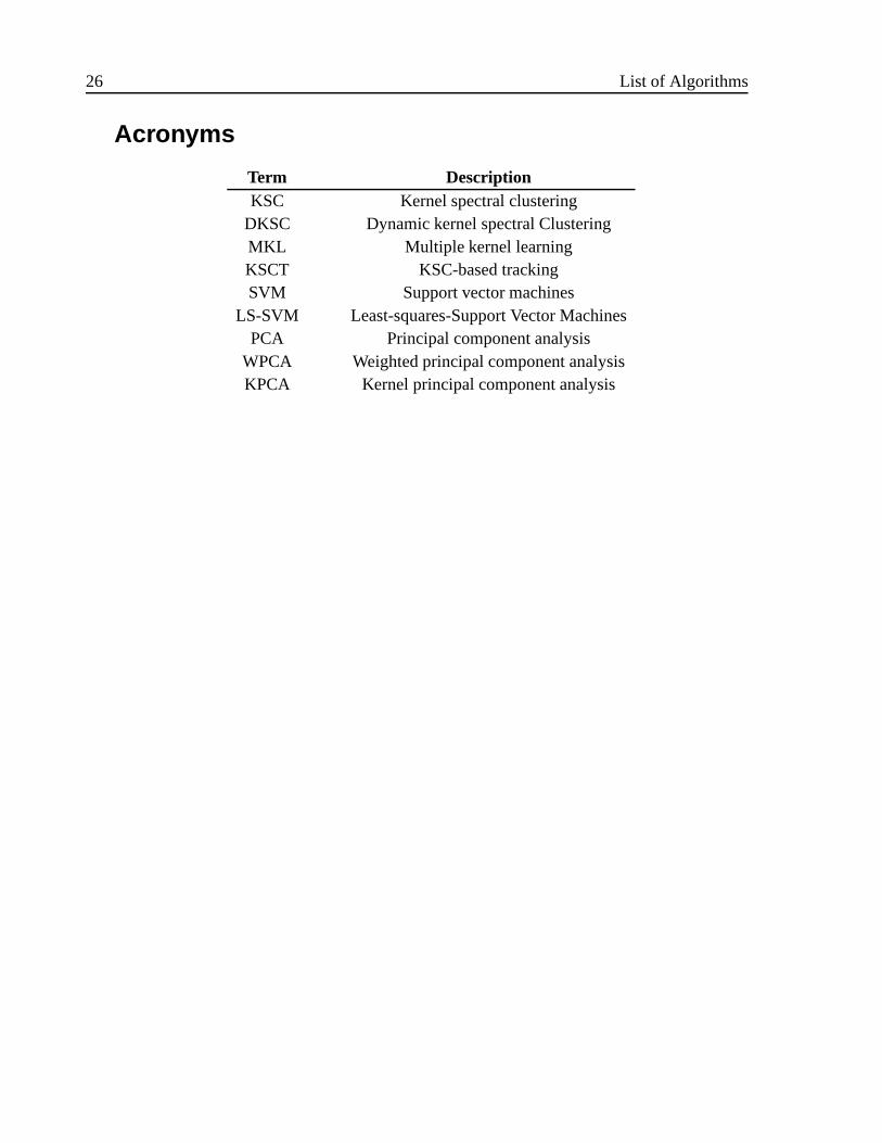
Acronyms
Term DescriptionKSC Kernel spectral clustering
DKSC Dynamic kernel spectral ClusteringMKL Multiple kernel learningKSCT KSC-based trackingSVM Support vector machines
LS-SVM Least-squares-Support Vector MachinesPCA Principal component analysis
WPCA Weighted principal component analysisKPCA Kernel principal component analysis

Part I.
Preliminaries
1. Introduction
In the field of pattern recognition and classification, the clustering methods derived fromgraph theory and based on spectral matrix analysis are of great interest because of theirusefulness for grouping highly non-linearly separable clusters. Some of its remarkable ap-plications to be mentioned are human motion analysis and people identification [1,2], imagesegmentation [3–5] and video analysis [6, 7], among others. The spectral clustering tech-niques carry out the grouping task without any prior knowledge –indication or hints aboutthe structure of data to be grouped– and then partitions are built from the information ob-tained by the clustering process itself. Instead, they only require some initial parameterssuch as the number of groups and a similarity function. For spectral clustering, particularly,a global decision criterion is often assumed taking into account the estimated probabilitythat two nodes or data points belong to the same cluster [8]. For this reason, this kind ofclustering can be easily understood from a graph theory view point where such probabilityis to be associated to the similarity among nodes.
Typically, clusters are formed in a lower dimensional space involving a dimensionality re-duction process. This is done preserving the relationship among nodes as well as possible.Most approaches that deal with this matter are founded on linear combinations or latentvariable models where the eigenvalue and eigenvector decomposition (here termed eigen-decomposition) of the normalized similarity matrix takes place. In other words, spectral clus-tering comprises all the clustering techniques using information of the eigen-decompositionfrom any standard similarity matrix obtained from the data to be clustered.
In general, these methods are of interest in cases where, because of the complex structure,clusters are not readily separable and traditional grouping methods fail. In the state of theart on unsupervised data analysis, we can find several approaches for spectral clustering.There are methods based on graph partitioning problems solved by a relaxed formulationthat generally becomes a NP-complete problem [9–15]. These methods exploit the infor-mation given by the eigen-decomposition under the premise that any space generated by theeigenvectors (eigen-space) is directly related to the clustering quality [12]. Then, since itis possible to obtain a discrete solution, the muli-cluster clustering approach has emerged,named k-way normalized cuts [8]. Achieving such discrete solution implies to solve anotherclustering problem, albeit in a lower dimension. Therefore, the eigenvectors can be consid-
1.1 Motivation and problem statement 3
ered as a new data set which can be grouped by means of a simple partitioning clusteringmethod such as K-means [10]. The approach described in [10] corresponds to a recursivere-grouping method. However, the big disadvantage of this method is that it only works wellwhen the information given by eigenvectors has a spherical structure [16]. Other works pro-pose minimizing the difference between unconstrained problem solutions and some groupindicators [17, 18] to find peaks and valleys of certain criterion capable of quantifying thegroup overlapping [19]. On the other hand, some spectral clustering approaches can be seenas particular cases of Kernel Principal Component Analysis (KPCA) as described in [20,21].The work presented in [21] shows that conventional spectral clustering based on binaryindi-cators, such asnormalized cut[10], NJW algorithm [12] and random walk-based methods [9]are variants of weighted KPCA regarding different affinity matrices.
1.1. Motivation and problem statement
In broad terms, clustering has shown to be a powerful technique for grouping and/or rank dataas well as a proper alternative for unlabeled problems. Due to its versatility, applicability andfeasibility, it has been preferred in many approaches. Nevertheless, despite several clusteringtechniques having been introduced, the selection and design of a grouping system is not atrivial task. Often, it is mandatory to analyze in detail the structure of data and the specificinitial conditions of the problem in order to group the homogenous data points. Besides, itmust be done in such a way that an accurate cluster recognition is accomplished.
One of the biggest disadvantages of the spectral clustering methods is that most of themhave been designed for analyzing only static data, that is to say, regardless of the temporaryinformation. Therefore, when data are changing along time, clustering can be performed onsingle current data frame without analyzing the previous ones. Some works have addressedthis important issue concerning applications such as human motion analysis [22,23]. Otherapproaches are focused on the design of dynamic kernels for clustering [24,25] as well as theuse of dynamic KPCA [26,27]. In the literature, many approaches prioritize the use of ker-nel methods since they allow to incorporate prior knowledge into the clustering procedure.However, the design of a whole kernel-based clustering scheme able to group time-varyingdata achieving a high accuracy is still an open issue.
This thesis presents the design of a kernel-based dynamic spectral clustering using a primal-dual approach so as to carry out the grouping task involving the dynamic information, that isto say, the changes of data frames along time. To this end, a dynamic kernel-based approachto extend a simple primal formulation to dynamic data analysis is introduced. This approachmay represent a contribution to pattern recognition mainly in applications involving time-varying information such as video analysis and motion detection, among others.

4 1 Introduction
1.2. Objectives
1.2.1. General objective
To develop a whole kernel-based clustering scheme using a primal-dual formulation forgrouping time-varying data.
1.2.2. Specific Objectives
* To propose a kernel spectral clustering approach with a proper selection and/or tuningof initial parameters to group both complex and simple data.
* To design a dynamic multiple kernel framework able to capture the evolutionary infor-mation in time-varying data.
* To develop a whole clustering scheme based on kernels for grouping time-varying dataframes via a primal-dual formulation.
1.3. Contributions of this thesis
This thesis was done within the framework of clustering, specifically, spectral clusteringbased on kernels, yielding the following main contributions to the state of art on this field:
• A new data projection to improve the performance of kernel spectral clustering is pro-posed. This projection consists of a linear mapping based on theM-inner productapproach, for which an orthonormal eigenvector basis is chosen as the projection ma-trix. Moreover, projection matrix is calculated over the spectrum of kernel matrix. Thestrength of this approach is that local similarities and global structure are used to re-fine the projection procedure by preserving the most explained variance and reaching aprojected space that improves the clustering performance within the KSC framework.Another advantage of the proposed data projection is that a more accurate estimationof the number of groups is provided. Since introduced projected KSC is derived froma support vector machine-based model, it can also be trained, validated, and tested ina learning framework using a model selection criterion.
• A novel tracking approach based on the eigenvector decomposition of the normalizedkernel matrix is proposed, which yields a ranking value for each single frame from theanalyzed input sequence. As a result, obtained ranking values present a direct rela-tionship with the underlying dynamic events contained in the sequence. This approachalso provides substantial information to estimate both the number of groups and theground truth.
1.4 Manuscript organization 5
• Based on a multiple kernel learning approach, namely a linear of combination of ker-nels, a dynamic kernel spectral clustering (DKSC) approach is introduced. DKSC,from a set of kernels representing to a data matrix sequence, perform the clusteringprocess over the input data using a cumulative kernel matrix obtained from the consid-ered MKL approach. The weighting factors or coefficient for linear combination arethose ranking values given by a proposed tracking approach. Then, proposed methodis able to cluster dynamic data taking into account the past information.
Also, this work achieved other additional contributions on related topics, which are notamong the main topics but still important in the field of clustering:
• Two novel alternatives to the conventional spectral normalized cut clustering (NCC)without using eigenvectors are introduced. One based on a piecewise heuristic searchto determine the nodes having maximum similarity. Another one that consists of avariation of the NCC formulation aimed to pose a relaxed quadratic problem, whichcan be easy solved, for instance, by means of a conventional quadratic programmingalgorithm. Both proposed methods spend lower computational cost in comparisonwith conventional spectral clustering methods and keep a comparable performance aswell.
• A new supervised index for clustering performance, named probability-based perfor-mance quantifier (PPQ) is introduced. PPQ is based on simple probabilities calculatedby relative frequencies and provides a relative value for each class from data base viathe Bayes’ rule.
1.4. Manuscript organization
The manuscript is divided into five parts, namely,I preliminaries,II methods,III experimentsand results,IV final remarks, andV appendices. It is composed by eight main chapters,which are organized as follows:
• Chapter2 is a brief state of the art on kernel-based clustering for dynamic data.
• In chapter3, the normalize cut clustering (NCC) criterion from a graph-partitioningpoint of view is presented, aimed to solving multi-cluster problems via an eigenvectordecomposition. Some alternatives to solve the NCC problem without using eigenvec-tors are introduced as well.
• One of the capital chapters is chapter4, in which the description of the kernel spectralclustering method is presented. Also, an optimal data projection for KSC is introduced.In addition, some definitions and basics about kernels are studied.

6 1 Introduction
• Chapter5 is the central chapter, which explains the dynamic version of KSC based onmultiple kernel learning (MKL). Also, a tracking approach is introduced.
• The experimental setup and results of this thesis are shown respectively in chapters6and7.
• In chapter8, the conclusions achieved with this work and future work are presented.
2. State of the art on spectralclustering and dynamic dataanalysis
Spectral clustering, just as any unsupervised technique, is a discriminative method, that is,it does not require prior knowledge about the classes for classification. As such, it performsthe grouping process using only the information within the data and, generally, some startingparameters such as the number of resulting groups or any other hint about the initial parti-tion. In this case, given that the spectral clustering is backed up by graph theory, the inputparameters for clustering algorithms are the number of groups and the similarity matrix. Theinitialization is an important stage in the unsupervised methods since most of them are sen-sitive to the starting parameters; this means that if the initial parameters are not adequate,algorithm convergence may fail by falling on a suboptimal solution quite distant from theglobal optimum. On the other hand, as mentioned above, the unsupervised methods carryout the clustering with the direct information given by the data. Thus, if the initial repre-sentation space is not discriminative enough under the clustering criteria, feature extractionand/or selection stages may be, in some cases, required.
Following, a brief theoretical background with a bibliographic scope on spectral clusteringbased on kernels is presented.
2.1. Spectral clustering
Clustering based on spectral theory is a relatively new focus for unsupervised analysis; al-though it has been used in several studies that prove its efficiency on grouping tasks, espe-cially in cases when the clusters are not linearly separable. This clustering technique hasbeen widely used in a large amount of applications such as circuit design [9], computationalload balancing for intensive computing [28], human motion analysis and people identifica-tion [1,2], image segmentation [3–5] and video analysis [6,7], among others. What makesspectral analysis applied to data clustering appealing is the use of the eigenvalue and eigen-vector decomposition in order to obtain the local optima closest to the global continuous
8 2 State of the art on spectral clustering and dynamic data analysis
optima.
The spectral clustering techniques take advantage of the topology of data from a non-directedand weighted graph-based representation. This approach is known as graph partitioning; init an initial optimization problem is usually posed formulated under some constraints. Oftenthis formulation is relaxed and then becomes a NP-complete problem [9–14]. In addition,the estimation of global optima in a relaxed continuous domain is done through the eigenvec-tor decomposition (eigen-decomposition) [8], based on the theorem by Perron - Frobenius,which establishes that largest strictly real eigenvalues associated to a positive definite andirreducible matrix determine their own spectral ratio [29]. In this case, such matrix corre-sponds to the affinity or similarity matrix containing the similarities among data points. Inother words, the space created by the eigenvectors in the affinity matrix is closely related tothe clustering quality.
Under this principle, and considering the possibility of obtaining a discreet solution througheigenvectors, there have been proposed multi-cluster approaches such as the k-way normal-ized cut method introduced in [8]. In such method, to obtain the discrete solution, anotheroptimization problem must be solved, albeit in a lower dimensional domain. Besides, lead-ing eigenvectors can be considered as a new data set that can be clustered by a conventionalclustering algorithm such as K-means [10, 30]. Then, a hybrid algorithm is achieved inwhich the spectral analysis algorithms may generate the eigenvector space and set adequateinitial parameters, while partitioning algorithms would be in charge of the clustering itself.This means that the spectral analysis can support the conventional techniques generatingan initialization improving the algorithm convergence. Nevertheless, similar to the hardmembership values obtained from some center-based clustering algorithms [31], a spectralclustering scheme can cluster data alone outputting a cluster binary matrix denoting the datapoint membership regarding each cluster. To carry out this clustering approach, not only arethe eigenvectors needed, but also is the orthonormal transformation of eigenvector solution(eigen-solution). This leads to the target of spectral clustering being the finding of the bestorthonormal transformation that generates an appropriate discretization of the continuoussolution [10].
In general, when dealing with bi-cluster problems, the solution of the relaxed problem is of-ten a specific eigenvector [16]. However, when the problem is within a kind of multi-clusterframework, determining relevant information for the clustering task based on the eigen-solution is not that simple. Among the approaches proposed to address the multi-way spec-tral clustering problem, we find recursive re-clustering methods (recursive-cuts) to obtain thecluster indicator vector as discussed in [10]. This approach is not optimal since it only takesinto consideration an eigenvector and discards the information from the remaining vectors,
2.2 Kernel-based clustering 9
which can also provide a clue as to the cluster conformation. The re-clustering approachamounts to applying a partitioning clustering method on the eigenvector space, although thisonly works properly when the eigen-space has a spherical structure [16]. In [30], authors pro-pose a simple clustering algorithm consisting of a conventional method to estimate the mostrepresentative data points, one per cluster. This is done through the eigen-decompositionof the normalized similiraty matrix. Subsequently, an amplitude–re-normalized eigenvectormatrix is obtained, which is clustered intoK subsets using the K-means algorithm. Finally,the data points are assigned to the corresponding clusters according to the geometric struc-ture of the initial data matrix.
A later work [8] presents a method for multi-cluster spectral clustering in amore detailedmanner, in which an optimization problem is posed to guarantee that the algorithm conver-gence lies within the global optimum region. To this end, two optimization sub-problems areformulated: one to obtain the global optimal values in an unconstrained continuous domainand another for getting a discrete solution corresponding to the continuos one. Unlike thealgorithm introduced in [30], this method does not require an additional clustering algorithmsince it generates a binary matrix on its own representing the data point membership. Inthis way each data point belong to an unique a cluster. In this study, orthonormal transfor-mations and singular value decomposition are employed to determine the optimal discretesolution, taking into consideration the principle of orthonormal invariance and the optimaleigen-solution criterion. Another study [32] applies the foundations from [8] and [30] toexplain theoretically the relationship between kernel K-means and spectral clustering, start-ing from the point of view of K-means objective function generalization towards obtaining aspecial case of the objective function able to solve the normalized cut (NC) problem. Then,a positive definite similarity matrix is assumed as well as algorithms based on local searchesand optimization formulations are performed to improve the clustering process regarding thekernel. This is done in such a manner that it might be satisfied the optimization conditionestablishing that NC-based clustering objective function must be monotonically decreasing.
2.2. Kernel-based clustering
More advanced approaches propose minimizing a feasibility measure between the solutionsof the unconstrained problem and the allowed cluster indicator [17, 18], finding peaks andvalleys of a cost function that quantifies the cluster overlapping [19]. Then, a discretiza-tion process is carried out. The problem of continuos solution discretization is formulatedand solved in [33]. There exist graph-based methods associated with normalized and non-normalized Laplacian, which provide relevant information contained in the Laplacian eigen-vector is of great usefulness for the clustering task. As well, they often provide a straight-
10 2 State of the art on spectral clustering and dynamic data analysis
forward interpretation about the clustering quality based ona random graph theory. Underthe assumption that data is a random weigthed graph, it is demonstrated that spectral clus-tering can be seen as a maximal similarity-based clustering. In [18], some alternatives tosolving open issues in spectral clustering are discussed, such as the selection of a properanalysis scale, extensions to multi-scale data management, the existence of irregular andpartially known groups, and the automatic estimation of the number of groups. The authorspropose a local scaling to calculate the affinity or similarity between each pair of data points.This scaled similarity improves the clustering algorithms in terms of both convergence andprocessing time. Additionally, taking advantage of the underlying information given byeigenvectors is suggested to automatically establish the number of groups. The output ofthis algorithm can be used as a starting point to initialize partitioning algorithms such asK-means. There are another approaches that have been pointed out to extend the clusteringmodel to new data (testing data), i. e., out-of-sample extension. For instance, the methodspresented in [34, 35] allow for extending the clustering process to new data, approximat-ing the eigen-function (a function based on the eigen-decomposition) using the Nystrom’smethod [36,37]. Therein, a clustering method and a searching criterion are typically chosenin a heuristic fashion.
Another spectral clustering perspective is the Kernel Principal Component Analysis (KPCA)[20, 21]. KPCA is an unsupervised technique for nonlinear feature extraction and dimen-sionality reduction [38]. Such method is a nonlinear version of PCA using positive definitematrices whose aim is to find the projected space onto an induced kernel feature space pre-serving the maximum explained variance [16]. The relationship between KPCA and spectralclustering is explained in [20, 21]. Indeed, the work presented in [21] demonstrates thatthe classical spectral clustering, such as normalized cut [10], the NJW algorithm [12] andrandom walk model [9] can be seen as particular cases of weighted KPCA, just with modifi-cations on the kernel matrix.
In [16], a spectral clustering model is proposed which is based on a KPCA scheme on the ba-sis of the approach proposed in [21] in order to extend it to multi-cluster clustering, whereincoding and decoding stages are involved. To that end, a formulation founded on least squaresmethod-based support vector machines (LSSVM) considering weighted versions [39, 40].This formulation aims to a constrained optimization problem in a primal-dual frameworkthat allows for extending the model to new isolated data without needing additional tech-niques (e. g. the Nystrom method). In this connection, a modified similarity matrix isproposed whose eigenvectors are dual regarding a primal optimization problem formulatedin a high dimensional space. Also, it is proven that such eigenvectors contain underlyingrelevant information useful for clustering purposes and display a special geometric structurewhen the resulting clusters are well formed -in terms of compactness and/or separability.
2.3 Dynamic clustering 11
The out-of-sample extensions are done by projecting cluster indicators onto the eigenvec-tors. As a model selection criterion, the method so-called Balanced Line Fit (BLF) criterionis proposed. This criterion explores the structure of the eigenvectors and their correspondingprojections, which can be used to set the initial model parameters.
Similarly, in [41], another kernel model for spectral clustering is presented.This method isbased on the incomplete Cholesky decomposition. It is able to deal efficiently with large-scale clustering problems. The set-up is made on the basis of a WPCA scheme based onkernels (WKPCA) from a primal-dual formulation. In it, the similarity matrix is estimatedby using the incomplete Cholesky decomposition.
2.3. Dynamic clustering
Dynamic data analysis is of great interest, there are several remarkable applications such asvideo analysis [42] and motion identification [43], among others. By using spectral analysisand clustering, some works have been developed taking into account the temporal infor-mation for the clustering task, mainly in segmentation of human motion [22, 23]. Otherapproaches include either the design of dynamic kernels for clustering [24,25] or a dynamickernel principal component analysis (KPCA) based model [26,27]. Another study [44] mod-ifies the primal functional of a KPCA formulation for spectral clustering to add the memoryeffect.
There exists another alternative known as multiple kernel learning (MKL), which has emergedto deal with different issues in machine learning, mainly, regarding support vector machines(SVM) [45, 46]. The intuitive idea of MKL is that learning can be enhanced when usingdifferent kernels instead of an unique kernel. Indeed, local analysis provided by each kernelis of benefit to examine the structure of the whole data when having local complex clusters.

Part II.
Methods
3. Normalized cut clustering
3.1. Introduction
The clustering methods based on graph partitioning are discriminative approaches to group-ing homogeneous nodes or data points without making assumptions about the global struc-ture of data, but local evidence on a pairwise relationship among data points is considered.Such relationship, known as similarity, defines how likely two data points are to belong tothe same cluster. Then, all data points are split into disjunct subgraphs or subsets accordingto a similarity-based decision criterion. Most of approaches apply such criterion on a lower-dimensional space representing the original one, preserving the relationships among nodesas accurately as possible. Then, within a relaxed formulation, some feasible continuous solu-tions can be obtained by eigenvector decompositions [8]. Indeed, eigenvectors can be inter-preted as geometric coordinates in order to directly cluster them by means of a conventionalclustering technique as suggested in [18,32]. Nonetheless, there are alternatives to achievethis clustering without using eigenvectors but taking advantages of multi-level schemes [47]or formulating easy-to-solve quadratic problems with linear constraints [15,48].
In this work, we give special attention to the multi-cluster spectral clustering (MCSC) intro-duced in [8], since it computes a discrete solution from the space spannedby the eigenvectorsregarding a certain orthonormal basis. Then, instead of using additional clustering stages,the MCSC generates some binary cluster indicators directly.
The scope of this chapter encompasses a detailed explanation, formulation and solutions forthe normalized cut clustering. We start mentioning some basics of graphs in section3.2.Then, the MCSC method is described in section3.3, by deriving a muti-cluster partitioningcriterion from a graph theory point of view, as shown in section3.3.1. The algorithm forMCSC is summarized in section3.3.3.
3.2. Basics of graphs
As mentioned above, a way to easily understand the spectral clustering methods is froma geometric perspective using graphs. In this section, some definitions around graphs arepresented as well as properties and operations needed for further analysis.

14 3 Normalized cut clustering
3.2.1. Graph
A graph is a non-empty finite set of nodes or data points, and edges connecting the nodespairwise. Then, a so-called graphG can be described by the ordered pairG = (V,E), whereV is the set of nodes andE is the set of edges.
3.2.2. Weighted graphs
A weighted graph can be represented asG = (V,E,Ω), whereΩ represents the relationamong nodes, in other words, the affinity or similarity matrix. Given thatΩi j represents theweight of the edge betweeni-th and j-th node, it must be a non-negative value. In addition,in a non-directed graph is verified thatΩi j = Ω ji . Therefore, matrixΩ must be chosen assymmetric and positive semidefinite. Figure3.1shows an example of a weighted graph.
1
2
3
Ω12 = Ω21 Ω23 = Ω32
Ω13 = Ω31
Ω11
Ω22
Ω33
Figure 3.1.:Weighted graph with three nodes
3.2.3. Properties and measures
There are several useful measures and applications of graphs. In this work, we focus on twofundamental measures, namely, the total weighted connections from a subgraph to anotherone, and the degree. Consider the graphG = (V,E,Ω) and its subgraphsVk,Vl ⊂ V. Thetotal weighted connections fromVk andVl is defined as:
links(Vk,Vl) =∑
i∈Vk, j∈Vl
Ωi j (3.1)
The degree of non-weighted graph regarding a certain node is the number of edges adjacentthereto. Instead, in cases of weighted graph the degree is the total weighted connections
3.3 Clustering Method 15
from a certain subgraph to the whole graph. Therefore, the degree ofVk can be calculatedas:
degree(Vk) = links(Vk,V) (3.2)
The degree is often used as a normalization term for connection weights so that we canestimate the ratio of weighted connections from a subgraph regarding another one. Forinstance, the ratio of weighted connections betweenVk andVl regarding the total connectionsfromVk is:
linkratio(Vk,Vl) =links(Vk,Vl)degree(Vk)
(3.3)
3.3. Clustering Method
In terms of clustering, the variableV = 1, · · · ,N represents the indexes of the data setto be grouped. Then, the aim of spectral clustering is to group theN data points fromVinto K disjoint subsets, so thatV = ∪K
l=1Vl andVl ∩ Vm = ∅, ∀l , m. Commonly, thisdecomposition is done by using spectral information and orthonormal transformations. Letus analyze two special linkratios: The first one is linkratio(Vk,Vk), which measures the ratioof links staying withinVk itself [8]. The second one is linkratio(Vk,Vk\V), which measuresthe ratio of links escaping fromVk, being a complement of the first one. According to this,a suitable clustering is then achieved when both maximizing connections within partitionsand minimizing connections between partitions. These two goals can be expressed as thek–way–normalized associations (knassoc) and normalized cut criteria (kncuts), which arerespectively as follows:
knassoc(ΓKV) =
1K
K∑
k=1
linkratio(Vk,Vk) (3.4)
and
kncuts(ΓKV) =
1K
K∑
k=1
linkratio(Vk,Vk\V) (3.5)
beingΓKV= V1, · · · ,VK the set containing all partitions.
Also, because a normalization term is applied, we can easily verify that
knassoc(ΓKV) + kncuts(ΓK
V) = 1 (3.6)

16 3 Normalized cut clustering
3.3.1. Multi-cluster partitioning criterion
From equation3.6, we can infer that maximizing the associations and minimizingthe cuts areachieved simultaneously. Therefore, the objective function to be maximized for clusteringpurposes is in the form:
ε(ΓKV) = knassoc(ΓK
V) (3.7)
3.3.2. Matrix representation
Henceforth, the partition setΓKV
is to be represented by a cluster binary indicator matrixM ∈ 0, 1N×K such thatM = [M1, . . . ,MK]. Matrix M holds the membership of eachdata point regarding a certain cluster, in such a way thatmik is the membership value of thedata pointi with respect to clusterk, so:
mik = ⌊i ∈ Vk⌋, i ∈ V, k ∈ [K] (3.8)
where [K] denotes the set of entire numbers ranged into the interval [1,K], mik is theik entryof matrixM , ⌊·⌋ is a binary indicator: it becomes 1 if the argument its true and 0 otherwise.Beside, since each node can only belong to one cluster, the conditionM1K = 1N must beguaranteed, where1d is ad-dimensional all ones vector. LetD ∈ RN×N be the degree matrixfor the similarity matrix defined as:
D = Diag(Ω1N) (3.9)
where Diag(·) denotes a diagonal matrix formed by the argument vector. Then, the measuresgiven by equations (3.1) and (3.3) can be also written as:
links(Vk,Vk) =MTk ΩMk (3.10)
and
degree(Vk) =MTk DMk (3.11)
According to the above, the multi-cluster partitioning criterion can be expressed as:
max ε(M ) =1K
K∑
k=1
MTk ΩMk
MTk DMk
(3.12)
s. t. M ∈ 0, 1N×K, M1K = 1N (3.13)
This the formulation for the normalized cut problem regarding the indicator matrixM ,termedNCPM.
3.3 Clustering Method 17
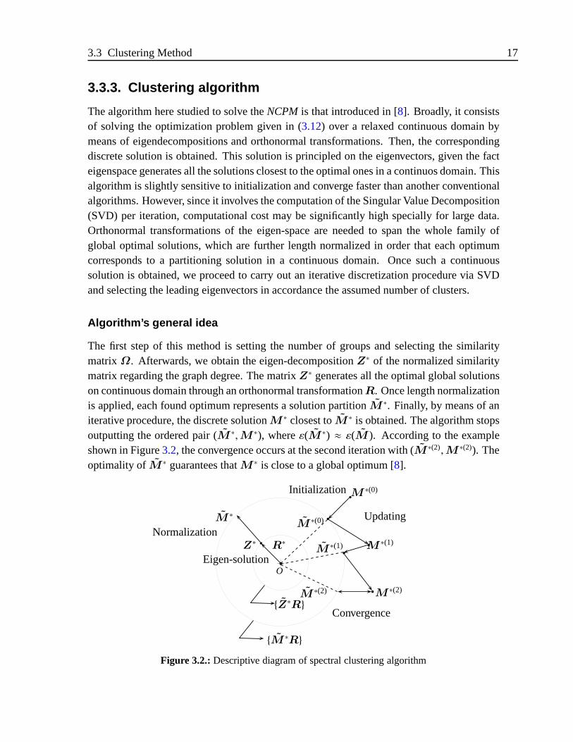
3.3.3. Clustering algorithm
The algorithm here studied to solve theNCPM is that introduced in [8]. Broadly, it consistsof solving the optimization problem given in (3.12) over a relaxed continuous domain bymeans of eigendecompositions and orthonormal transformations. Then, the correspondingdiscrete solution is obtained. This solution is principled on the eigenvectors, given the facteigenspace generates all the solutions closest to the optimal ones in a continuos domain. Thisalgorithm is slightly sensitive to initialization and converge faster than another conventionalalgorithms. However, since it involves the computation of the Singular Value Decomposition(SVD) per iteration, computational cost may be significantly high specially for large data.Orthonormal transformations of the eigen-space are needed to span the whole family ofglobal optimal solutions, which are further length normalized in order that each optimumcorresponds to a partitioning solution in a continuous domain. Once such a continuoussolution is obtained, we proceed to carry out an iterative discretization procedure via SVDand selecting the leading eigenvectors in accordance the assumed number of clusters.
Algorithm’s general idea
The first step of this method is setting the number of groups and selecting the similaritymatrixΩ. Afterwards, we obtain the eigen-decompositionZ∗ of the normalized similaritymatrix regarding the graph degree. The matrixZ∗ generates all the optimal global solutionson continuous domain through an orthonormal transformationR. Once length normalizationis applied, each found optimum represents a solution partitionM ∗. Finally, by means of aniterative procedure, the discrete solutionM ∗ closest toM ∗ is obtained. The algorithm stopsoutputting the ordered pair (M ∗,M ∗), whereε(M ∗) ≈ ε(M ). According to the exampleshown in Figure3.2, the convergence occurs at the second iteration with (M ∗(2),M ∗(2)). Theoptimality ofM ∗ guarantees thatM ∗ is close to a global optimum [8].
b
O
Z∗R
M ∗R
M ∗(2)
M ∗(1)M ∗(1)
M ∗(2)
M ∗(0)
M ∗(0)M ∗
Z∗
Convergence
Updating
Initialization
Normalization
Eigen-solutionR∗
Figure 3.2.:Descriptive diagram of spectral clustering algorithm
18 3 Normalized cut clustering
Solving the optimization problem
In this section, some particular details of the optimization problem solution for spectral clus-tering are outlined. As mentioned above, the problem can be solved in two stages, as follows:First, the continuos global optimum is found. Second, discrete solution closest to that deter-mined in the first stage is calculated.The convergence to a continuos global optimum is guaranteed through an orthonormal trans-formation of the eigenvectors of normalized similarity matrix, therefore writing the optimiza-tion problem in terms ofZ∗ is of usefulness. To this end, defineZ as the scaled partitionmatrix [49], which corresponds to scaling the matrixM in the form
Z =M (MTDM )−12 . (3.14)
SinceMTDM is a diagonal matrix, the columns ofZ correspond to the columns ofMscaled by the inverse root square of the degree of matrixΩ. Then, it is possible to saythat one of the conditions that feasible solutions for the optimization problem must satisfyis: ZTDZ = IK, whereIK is the identity matrix in sizeK × K. By omitting the initialconstraints, a new optimization problem in terms of matrixZ can be posed, so:
max ε(Z) =1K
tr(ZTΩZ) (3.15)
s. t. ZTDZ = IK (3.16)
The fact of using the variableZ over a relaxed continuos domain makes that the discreteoptimization problem turns to a continuos one easy to solve. To solve the latter probleminvolves taking into into account two special propositions: orhonormal invariance and opti-mal eigensolution. Hereinafter, the continuos NC problem in terms ofZ is to be denoted asNCPZ.
Proposition 3.3.1. (Orthonormal Invariance) Let R ∈ RK×K a rotation matrix andZa possible solution for NCP, thenZR is also a solution whenRTR = IK. Likewise,ε(ZR) = ε(Z), which means that they have the same objective function value.
Indeed, ifR is orthonormal it is easy to prove that
tr((ZR)TΩ(ZR)) = tr(RTZΩZR) = tr(ZTΩZ)
Therefore, despite an arbitrary orthonormal rotation, all the feasible solutions forNCPZkeepthe same properties. In other words, all of them are equally likely to be considered as a globaloptimum. In proposition3.3.2, a newNCPZapproach is posed aimed to solve the problem
3.3 Clustering Method 19
by an eigensolutionZ∗ aswell as prove that the eigenvectors of the normalized similaritymatrix are among the global optima. Let us define the normalized similarity matrixP as:
P =D−1/2ΩD−1/2 (3.17)
Matrix P is stochastic [50], thus we can easily verify that1N is a trivial eigenvector ofPassociated to the largest eigenvalue, which is 1 due to the normalization regarding the degree.
Proposition 3.3.2. (Optimal eigensolution) Let (V ,S) be the eigen-decomposition ofP ,such that:
PV = V S, V = [v1, . . . , vN] andS = Diag(s)with eigenvalues ordered decreasingly, so that s1 ≥, . . . ,≥ sN .
Such decomposition can be done from the orthonormal eigen-solution(V ,S) associated toD− 1
2ΩD− 12 where
V =D− 12 V (3.18)
and
D− 12ΩD− 1
2 V = V S, V TV = IN. (3.19)
Then, any subset formed by K eigenvectors is a local optimum of NCPZ as well as the firstK vectors determine the global optimum.
Now, we can write the objective function value of the subsets to be solutions forNCPZas:
ε[vπ1, . . . , vπK] =1K
K∑
k=1
sπk (3.20)
whereπ is an index vector ofK distinct integers from [N] = 1, . . . ,N. Then, in accordanceto the Proposition3.3.2, global optima are obtained withπ = [1, . . . ,K], as follows:
Z∗ = [v1, . . . , vK] (3.21)
whose eigenvalues and objective value are respectively:
Λ∗= Diag([s1, . . . , sK]) (3.22)
ε(Z∗) =1K
tr(Λ∗) = maxZTDZ=IK
ε(Z) (3.23)
Summarizing, the global optimum ofNCPZis a subspace spanned by the eigenvectors asso-ciated to the largestK eigenvalues ofP through orthonormal transformations in the form:
ZTR : RTR = IK,PZ∗ = ZΛ∗ (3.24)
Solutions forNCPMare upper bounded by the objective function value of the solutionsZ∗R.
20 3 Normalized cut clustering
Corollary 3.3.1. (Upper bounding) For any K (K≤ N), we have that
maxε(ΓKV) ≤ max
ZTDZ=IK
ε(Z) =1K
K∑
k=1
sk (3.25)
In addition, the optimal solution forNCPZdisminuye conforme se aumente el numero degrupos considerados.
Corollary 3.3.2. (Decreasingly Monotonicity) For any K (K≤ N), we have that
maxZTDZ=IK+1
ε(Z) ≤ maxZTDZ=IK
ε(Z) (3.26)
Once eigen-solution is obtained, spaceZ is transformed to retake the initial problem. There-fore, if T(·) is a function for mapping fromM to Z, thenT−1 is the normalization ofM inthe form:
Z = T(M ) =M (MTDM )−12 (3.27)
and
M = T−1(Z) = Diag( diag−12 (ZZT))Z (3.28)
where diag(·) represents a vector formed by the diagonal entries of the argument matrix.From a geometric point of view, by assuming the rows of matrixZ as coordinates from aK-dimensional space, we can infer thatT−1 is a length normalization doing that all the pointslie on the unit hypersphere centered at the origin. In this way, we transform a continuousoptimumZ∗R from theZ-space to theM -space. Since matrixR is orthonormal, we canverify that:
T−1(Z∗R) = T−1(Z∗)R (3.29)
Previous simplification allows to directly characterize the continuos optima throughT−1(Z∗)on theM -space, as follows:
M ∗R : M = T−1(Z∗),RTR = IK (3.30)
The second stage to etapa to solveNCPM is calculating the optimal discrete solution. Ingeneral, the optima ofNCPZare non-optimum solutions forNCPM [8]. Nevertheless, theyare useful for determining a nearby discrete solution. Such solution may not be the abso-lute maximizer ofNCPM but it is close to the global optimum due to the continuity of theobjective function. Then, the discretization process is aimed to finding a discrete solutionsatisfying the binary conditions given by the initial formulation in equations (3.8) and (3.13).This is done in such a way that the found solutions are close to the continuos optimum, asdescribed in (3.30).
3.3 Clustering Method 21
Theorem 3.3.1.(Optimal discretization) An optimal discrete partitionM ∗ is that satisfyingthe following optimization problem, termed OPD (Optimal discretization problem), in theform:
min φ(M ,R) = ‖M − M∗R‖2F (3.31)
s. t. M ∈ 0, 1N×K , M1K = 1N, RTR = IK (3.32)
where‖A‖F denotes the Frobenius’s norm of matrixA, such that: ‖A‖F =√
tr(AAT).Then, a local optimum(M ∗,R∗) can be iteratively solved by dividing OPD into two sub-problems: ODPM and ODPR, which respectively correspond to the optimization problemaformulation in terms ofM andR, so:
Optimization problem formulated by assumingR∗ known (ODPM) is:
min φ(M ) = ‖M − M ∗R‖2F (3.33)
s. t. M ∈ 0, 1N×K , M1K = 1N. (3.34)
Likewise, whenM ∗ is known (ODPR), we have
min φ(R) = ‖M − M ∗R‖2F (3.35)
s. t. RTR = IK (3.36)
The optimal solution for ODPM can be obtained by selecting the K eigenvectors associatedto the K largest eigenvalues:
m∗il = 〈l = arg minj
mi j 〉, j ∈ 1, . . . ,K, i ∈ V (3.37)
as well as the solution for ODPR can be reached through the singular values, as follows:
R∗ = UUTM ∗T= UΣUT, Σ = Diag(ω) (3.38)
where(U ,Σ, U ) is the singular value decomposition ofX∗TX∗, withUTU = IK , UTU =
IK andω1 ≥, . . . ,≥ ωK.
Proof. The objective function can extended in the form
φ(M ,R) = ‖M ∗ − MR‖2F = ‖M‖2F + ‖M‖2F − tr(MRTM +MTMR) =2N − 2 tr(MRTM ∗T),
what means that minimizingφ(M ,R) is equivalent to maximizing tr(MRTM ∗T). There-fore, in case ofODPM, since all the entries of diag(MR∗TM ∗T) can be independently
22 3 Normalized cut clustering
optimized, equation (3.37) is demonstrated. To demonstrate the solution forODPR, we canform the corresponding Lagrangian using as multiplier the symmetric matrixΛ, so:
L(R,Λ) = tr(M ∗RTM ∗T) − 12
tr(ΛT(RTR − IK)), (3.39)
where the optimum (R∗,Λ∗) must satisfy:
LR = M ∗TM ∗ −RΛ = 0⇒ Λ∗= R∗TM ∗TM ∗ (3.40)
Finally, becauseΛ∗ = UΣUT, R∗ = UUT, φ(R) = 2N − 2 tr(Σ) and the greatest value oftr(Σ) generates the matrixM ∗ nearest toM
∗R∗.
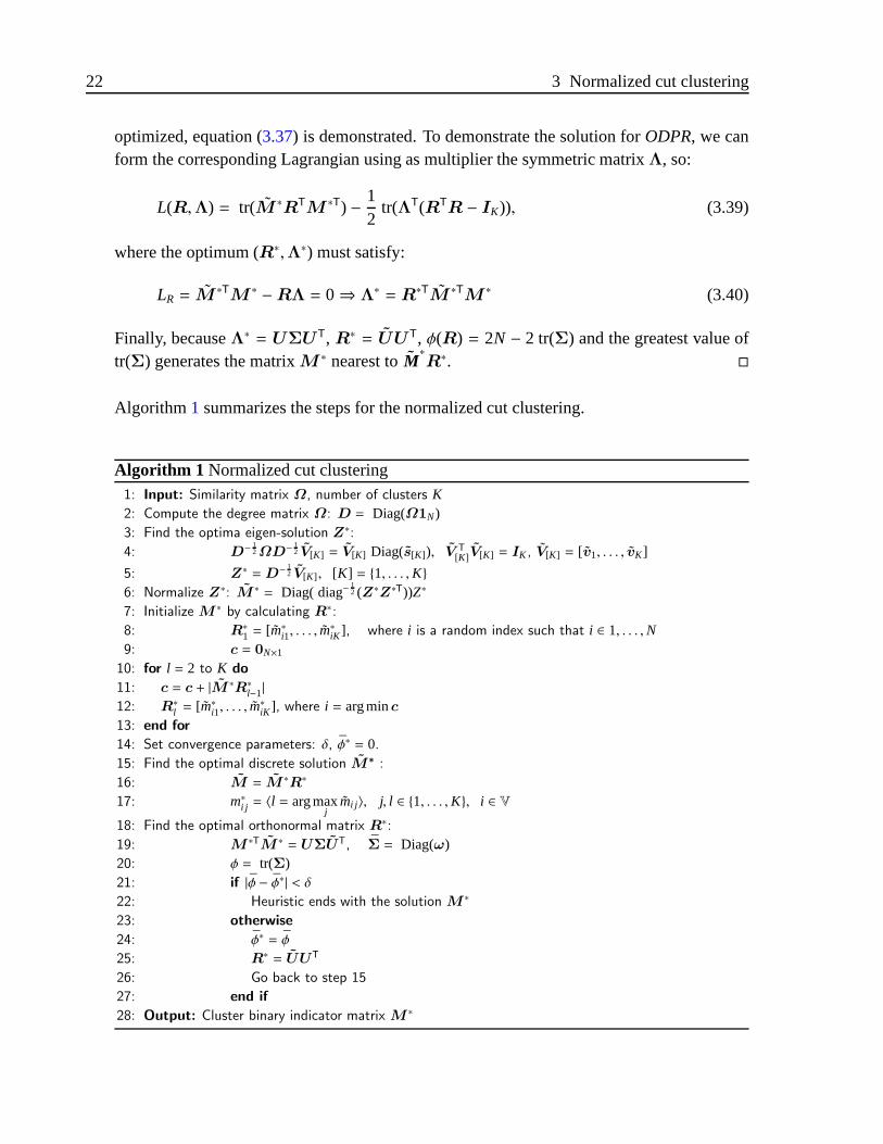
Algorithm 1 summarizes the steps for the normalized cut clustering.
Algorithm 1 Normalized cut clustering1: Input: Similarity matrix Ω, number of clusters K2: Compute the degree matrix Ω: D = Diag(Ω1N)3: Find the optima eigen-solution Z∗:
4: D− 12ΩD− 1
2 V[K] = V[K] Diag(s[K]), V T[K]V[K] = IK , V[K] = [v1, . . . , vK ]
5: Z∗ =D− 12 V[K] , [K] = 1, . . . ,K
6: Normalize Z∗: M ∗= Diag( diag−
12 (Z∗Z∗T))Z∗
7: Initialize M ∗ by calculating R∗:
8: R∗1 = [m∗i1, . . . , m∗iK ], where i is a random index such that i ∈ 1, . . . ,N
9: c = 0N×1
10: for l = 2 to K do
11: c = c + |M ∗R∗l−1|12: R∗l = [m∗i1, . . . , m
∗iK ], where i = arg minc
13: end for
14: Set convergence parameters: δ, φ∗ = 0.15: Find the optimal discrete solution M ∗ :
16: M = M ∗R∗
17: m∗i j = 〈l = arg maxj
mi j 〉, j, l ∈ 1, . . . ,K, i ∈ V18: Find the optimal orthonormal matrix R∗:
19: M ∗TM ∗= UΣUT, Σ = Diag(ω)
20: φ = tr(Σ)21: if |φ − φ∗| < δ22: Heuristic ends with the solution M ∗
23: otherwise
24: φ∗ = φ
25: R∗ = UUT
26: Go back to step 15
27: end if
28: Output: Cluster binary indicator matrix M ∗
3.4 Proposed alternatives to solve the NCC problem without using eigenvectors 23
Summarizing, iteratively solution forOPD into two stages is as follows: First, the estima-tion of discrete optimumM ∗R (by solvingODPR) is found. Second, determining the mostsuitable orthonormal transformation withODPM). Then, heuristic is iterated until conver-gence. Both stages use the same objective functionφ but they have different restrictions.Due to the iterative nature, this method can only guarantee the convergence to a local opti-mum. Nonetheless, convergence can be enhanced through setting proper initial parametersin both performance and speed. It is also important to mention that this is method is rea-sonably robust to the random initialization due to the orthonormal invariance of continuosoptima [8].
3.4. Proposed alternatives to solve the NCC problemwithout using eigenvectors
We introduce two novel approaches to solve the NCC problem: one by means of an heuristicsearch3.4.1and another one based on a quadratic problem formulation3.4.2.
3.4.1. Heuristic search-based approach
Perhaps, one of the most frequently used spectral clustering technique is the well-known nor-malized cut clustering (NCC). Mostly, approaches to deal with the NCC problem have beenaddressed to yield a dual problem, that is solved by means of an eigen-decomposition. Forinstance, K-means generalizations [51] and variations [18] based on kernels usually calledkernel K-means. Also, there exist approaches that solve the graph partitioning problem bymeans of a minimum cut formulation [10] or by using a dual formulation deriving into aquadratic problem and determining clustering indicators for multi-cluster spectral cluster-ing (MCSC) [8]. Nonetheless, because of the high computational cost that often involvesthe computation of eigenvectors, some studies have concerned about getting alternativesfor solving the normalized cut clustering without using eigenvectors such as multilevel ap-proaches with weighted graph cuts [47], and quadratic problem formulations with linearconstrains [15,48].Here, we propose a heuristic search carried out over the representation space given by thesimilarities among data points. Our method is a lower computational cost alternative toMCSC methods based on eigenvector decompositions, that is a MCSC method based ona heuristic search, termed MCSChs. Proposed MCSChs significantly outperforms con-ventional spectral clustering methods for solving the NCC problem in terms of speed andachieves comparable performance results as well. The foundation of our method lies in de-riving a new simple objective function by re-writing the quadratic expressions for MCSC [8]in such a way that we can intuitively design a searching process on the similarity represen-
24 3 Normalized cut clustering
tation space. Also, in order to avoid that the final solution leads to a trivial solution whereall elements are belonging to the same cluster, we propose both to incorporate prior knowl-edge, i.e., by taking advantage of the original labels to set initial data points for starting thegrouping process as well as an initialization stage to guarantee proper initial nodes.
Solution of NCC problem
As explained before, the NCC problem can be expressed as:
maxM
1K
tr(M⊤ΩM )tr(M⊤DM )
; s. t. M ∈ 0, 1N×K, M1K = 1N
Let us considere the following mathematical analysis. LetH ∈ RK×K such thatH =
M⊤DM , then, each corresponding entryi j is
hi j = (m1i, . . . ,mNi)
d1 0 · · · 00 d2 · · · 0...
.... . .
...
0 0 · · · dN
m1 j
m2 j...
mN j
= (m1id1,m2id2, . . . ,mNidN)
m1 j
m2 j...
mN j
=
N∑
s=1
msims jds
whereD = Diag(d) andd = [d1, . . . , dN] = Ω1N. Then,
tr(M⊤DM ) =K∑
i=1
hii =
K∑
i=1
N∑
s=1
m2sids =
K∑
i=1
(m2
1id1 +m22id2 + · · · +m2
NidN
)=
N∑
i=1
di
butdi =N∑
j=1Ωi j and therefore:
tr(M⊤DM ) =N∑
i=1
N∑
j=1
Ωi j = ||Ω||L1= const. (3.41)
Now, letG ∈ RN×N be an auxiliary matrix such thatG =M⊤ΩM , then, each entryi j of Gis:
gi j = (m1i, . . . ,mNi)Ω
m1 j...
mN j
=
N∑
t=1
mtiΩt1,
N∑
t=1
mtiΩt2, . . . ,
N∑
t=1
mtiΩtN
m1 j...
mN j
=
N∑
s=1
ms j
N∑
t=1
mtiΩts =
N∑
s=1
ms j
N∑
t=1
mt jωts =
N∑
s=1
ms j
N∑
t=1
mt jωts
3.4 Proposed alternatives to solve the NCC problem without using eigenvectors 25
Therefore,
tr(M⊤ΩM
)=
K∑
i=1
gii =
K∑
i=1
N∑
s=1
N∑
t=1
ms jmtiΩts
=
K∑
i=1
N∑
s=1
msi (m1iΩ1s+m2iΩ2s + · · · +mNiΩNs)
=
K∑
i=1
m1i (m1iΩ11 +m2iΩ21 + · · · +mNiΩN1)
+m2i (m2iΩ12 +m2iΩ22 + · · · +mNiΩN2) + . . .
+mNi (m1iΩ1N +m2iΩ2N + · · · +mNiΩNN)
In addition, since matrixΩ is symmetric, we have:
tr(M⊤ΩM
)=Ω11
K∑
i=1
m21i + Ω21
K∑
i=1
(m1im2i +m2im1i) + · · · + ΩNN
K∑
i=1
m2Ni
Considering that
K∑
i=1
m2ni = 1 ∀n ∈ [N],
we can write
tr(M⊤ΩM
)=Ω11 + Ω22 + · · · + ΩNN + 2
∑
p>q
N∑
i=1
Ωpqmpimqi
tr(M⊤ΩM
)= tr (Ω) + 2
∑
p>q
Ωpqδpq (3.42)
where
δpq =
1 if p′ = q′
0 if p′ , q′(3.43)
Notice thatδpq becomes 0 in case of the dot product between the rowst ands equals to 0,i.e., when such rows are linearly independent. Otherwise, it yields 0 pointing out that rowvectors are the same -containing 1 in the same entry. Finally,according to eq.3.42, sincetr(Ω) is constant, the term to be maximized is plainly
∑p>qΩpqδpq.
Heuristic Search based on Normalized Cut Clustering
In order to solve the NCC problem, an approach is proposed, named NCChs, by using priorknowledge about the known data labeling and a pre-clustering stage to heuristically cluster
26 3 Normalized cut clustering
the input data. Then, our method can be divided into three main stages, namely, grouping byan heuristic search, initial nodes setting, and pre-clustering.
- Prior knowledge stage
By maximizing∑
p>qΩpqδpq, the solution may lead to a trivial solution in which all elementsare belonging into the same cluster. In order to avoid this drawback, we propose to incorpo-rate prior knowledge, i.e., by employing the original labels, to assign the membership ofKdata points (one per class) into matrixM . Therefore, clusters are assigned according to themaximum value of similarity but preserving theK initial seed nodes belonging to respectiveclusters. This can be easily done by setting the entrymik representing the prior nodes to be1, and 0 for the remaining entries on the same rowi.
- Pre-clustering Stage
Also, in order to avoid wrongly assigning closer data points belonging to different clusters,we firstly carry out a pre-clustering process, where a relatively low percentage of the wholedata set (ǫ) is added to the seed nodes whose value of similarity is maximum, then theremaining data points are added in accordance to maximum similarity value between itselfand any of the previously assigned elements or the seed nodes. Denote the indexes related toinitial nodes asq = (q1, . . . , qK) whereqk ∈ V. After the initial nodes are assigned, we seekfor theǫ% of data points per node with maximum similarity and these are assigned to theirrespective node. In this manner, the initialK seed clusters are formed.
- Heuristic search
Once the pre-clustering stage is done, we haveK initial clusters. The remaining data pointsare assigned in accordance to the maximum similarity value between itself and any of thepreviously assigned data points. The proposed heuristic to form the final clusters works asfollows. Each time that an entryΩi j is chosen as the maximum similarity in the actual iter-ation, it is then removed by settingΩi j = 0 in order to avoid taking it into consideration forthe next iteration, and so on. This assignment process is done until all the data points arebelonging into any cluster, in other words,
∑Ni=1
∑Kk=1 mik = ||M ||L1 = N. Note that we can
employL1-norm since all entries ofM are positive. A graphic explanation of the search isshown in Figure3.3.
3.4 Proposed alternatives to solve the NCC problem without using eigenvectors 27
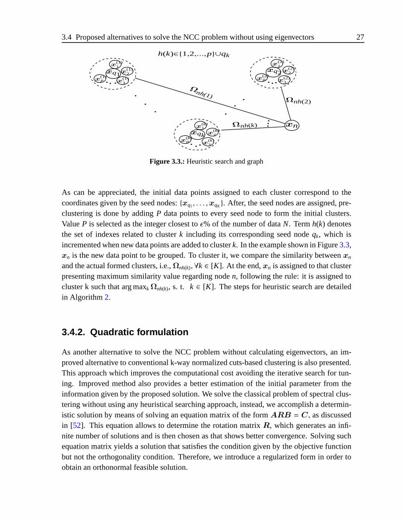
b
b
bb
b
b
b
bb
xq1xq2
bb b
bb
b
b b b
x(1)1
xqk
x(1)p
x(1)2
x(1)3
x(2)1
x(2)p
x(2)2
x(2)3
x(k)1
x(k)p
x(k)2
x(k)3
xn
Ωnh(2)
Ωnh(1)
Ωnh(k)
h(k)∈1,2,...,p∪qk
Figure 3.3.:Heuristic search and graph
As can be appreciated, the initial data points assigned to each cluster correspond to thecoordinates given by the seed nodes:xq1, . . . ,xqK . After, the seed nodes are assigned, pre-clustering is done by addingP data points to every seed node to form the initial clusters.ValueP is selected as the integer closest toǫ% of the number of dataN. Termh(k) denotesthe set of indexes related to clusterk including its corresponding seed nodeqk, which isincremented when new data points are added to clusterk. In the example shown in Figure3.3,xn is the new data point to be grouped. To cluster it, we compare the similarity betweenxn
and the actual formed clusters, i.e.,Ωnh(k),∀k ∈ [K]. At the end,xn is assigned to that clusterpresenting maximum similarity value regarding noden, following the rule: it is assigned tocluster k such that arg maxk Ωnh(k), s. t. k ∈ [K]. The steps for heuristic search are detailedin Algorithm 2.
3.4.2. Quadratic formulation
As another alternative to solve the NCC problem without calculating eigenvectors, an im-proved alternative to conventional k-way normalized cuts-based clustering is also presented.This approach which improves the computational cost avoiding the iterative search for tun-ing. Improved method also provides a better estimation of the initial parameter from theinformation given by the proposed solution. We solve the classical problem of spectral clus-tering without using any heuristical searching approach, instead, we accomplish a determin-istic solution by means of solving an equation matrix of the formARB = C, as discussedin [52]. This equation allows to determine the rotation matrixR, which generates an infi-nite number of solutions and is then chosen as that shows better convergence. Solving suchequation matrix yields a solution that satisfies the condition given by the objective functionbut not the orthogonality condition. Therefore, we introduce a regularized form in order toobtain an orthonormal feasible solution.

28 3 Normalized cut clustering
Algorithm 2 Heuristic Search for Clustering with prior knowledge and pre-clustering
1: Input: K, Ω, q, ǫ
2: Set P in accordance to ǫ% of N
3: M = 0N×K being 0N×K an all-zeros matrix of size N × K.
4: mqkk = 1; ∀ k ∈ [K]
5: c = [q1, . . . , qK]6: for i = 1 to P do
7: for h = 1 to K do
8: i = max argΩiqh
9: mih = 110: Ωiqh = 011: Ωqhi = 0
12: c = [c, i]13: end for
14: end for
15: while ||M ||L1 < N do
16: i, j = max argΩi j
17: while j < c do
18: ifK∑
k=1mik = 0 then
19: ℓ = argc == j20: mj = mℓ; Ωi j = 021: c = [c, j]22: end if
23: end while
24: end while
25: Output: M
Clustering method
Again, recalling the well-knownk-way normalized cut-based clustering, described:
max=1K
tr(M⊤ΩM )tr(M⊤DM )
(3.44a)
s. t.M ∈ 0, 1N×K, M1K = 1N (3.44b)
In order to guarantee thatM becomes binary it is needed that||M ||2F= tr(M⊤M ) =
tr(E) = n, whereE is a total adjacency matrix given byE = Diag(∑n
i=1 mi1, · · · ,∑n
i=1 miK ).Therefore, theNCPMoptimization problem can be expressed as:
max= tr(M⊤ΩM ) s. t. tr(M⊤DM ) = const., M1K = 1N (3.45)
3.4 Proposed alternatives to solve the NCC problem without using eigenvectors 29
Proposed NCPM Solution based on an One Iteration Tuning
The NCPM optimization problem can be relaxed as follows. LetP = D−1/2ΩD−1/2 be anormalized affinity matrix. Then, a relaxedNCPMversion can be expressed as:
max tr(L⊤PL), s. t. L⊤L = IK (3.46)
whereL =D−1/2M .A feasible solution to this problem isL∗ = VKR, whereVK is any orthonormal basis of theK-dimensional principal subspace ofP , andR is an arbitrary rotation matrix. At the end, abinarization process must be applied, e.g., by employing the sign function. Thus, there existsan infinite number of solutions. To overcome this issue with the aim to reach a deterministicsolution without using an iterative algorithm, the following mathematical development isdone. According to the constraint given in (C.1b), we have:
M1K =D1/2L1K =D1/2VKR1K = 1N (3.47)
Therefore, a possible rotation matrixR can be chosen asR = 1/K2V ⊤K D−1/2
1N1⊤K. Yet,
the previous solution do not satisfy the orthonormal condition given by (3.46), since it holdsthatR⊤R = K
ND−1, IK , and thus,R⊤ , R−1. Then, as a way to avoid this drawback, a
constrained optimization problem is introduced:
min ||VKR1K −D−1/21N||2F , s. t.R⊤R = IK (3.48)
where|| · ||F stands for Frobenius norm.
For the sake of simplicity, let us defineA = VK, B = 1K, C = D−1/2. Also, we intro-duce a regularized orthonormal matrixR = R + αIK to be determined that guarantees theorthogonality condition. Then, the optimization problem is rewritten as:
min ||ARB −C ||2F, s. t. R⊤R = IK ∴ ||R⊤R − IK ||2F = 0 (3.49)
By only considering the objective function to be minimized, the two following solutionsare possible [52]: vec(R) = [B⊤ ⊗ A]† vec(C) whereB† represents the pseudo-inversematrix ofB, and a real non-negative definite solution. The latter solution, in its easiest form,is given byR = A−CB− + Y − A−AY BB− requiring that theBen-Israel and Gevillecondition be satisfied [53], where theK × K dimensional matrixY is arbitrary andA−
denotes the inner inverse ofA, such thatAA−A = A. Moreover, both solutions turn out tobe no orthogonal and cannot be directly applied. Then, theGram-Schmidtorthogonalizationprocedure is, perhaps, the most intuitive solution. But, despite the orthogonal condition besatisfied, however, the original problem remains unsolved, i.e, there is no a solution that

30 3 Normalized cut clustering
satisfies the relaxed problem. Instead, we propose a solution based on Lagrange multipliers,as follows. The Lagrangian corresponding to the problem (3.49) is written as follows:
L(λ,R) = f (α,R) +K∑
k=1
λkgk(α,R) (3.50)
where
f (α,R) = tr((ARB −C)⊤(ARB −C)
)
K∑
k=1
λkgk(α,R) = tr((RTR − IK)⊤(R⊤R − IK)∆
)
Then, by solving∂ f∂R= 0 and ∂
∂R
(∑Kk=1 λkgk(α,R) = tr( ∂ f
∂R)), we obtain:
R = 2αA⊤CB† − IK (3.51a)
λ =12
diag
((R + (α − 1)IK)−1 ∂ f
∂R
)(3.51b)
where∆ = Diag(λ), B† denotes the pseudo-inverse matrix ofB andλ is the vector ofLagrange multipliers. At the end, a continuous estimation of matrixM can be written asM = D1/2L = D1/2VKR, which is further binarized to determine the initial clusteringproblem solutionM . Parameterα is chosen at the minimal point ofL, i.e., where bothfandg are minimum.
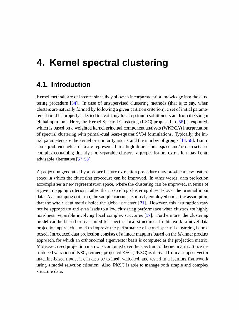
4. Kernel spectral clustering
4.1. Introduction
Kernel methods are of interest since they allow to incorporate prior knowledge into the clus-tering procedure [54]. In case of unsupervised clustering methods (that is to say, whenclusters are naturally formed by following a given partition criterion), a set of initial parame-ters should be properly selected to avoid any local optimum solution distant from the soughtglobal optimum. Here, the Kernel Spectral Clustering (KSC) proposed in [55] is explored,which is based on a weighted kernel principal component analysis (WKPCA) interpretationof spectral clustering with primal-dual least-squares SVM formulations. Typically, the ini-tial parameters are the kernel or similarity matrix and the number of groups [18,56]. But insome problems when data are represented in a high-dimensional space and/or data sets arecomplex containing linearly non-separable clusters, a proper feature extraction may be anadvisable alternative [57,58].
A projection generated by a proper feature extraction procedure may provide a new featurespace in which the clustering procedure can be improved. In other words, data projectionaccomplishes a new representation space, where the clustering can be improved, in terms ofa given mapping criterion, rather than providing clustering directly over the original inputdata. As a mapping criterion, the sample variance is mostly employed under the assumptionthat the whole data matrix holds the global structure [21]. However, this assumption maynot be appropriate and even leads to a low clustering performance when clusters are highlynon-linear separable involving local complex structures [57]. Furthermore, the clusteringmodel can be biased or over-fitted for specific local structures. In this work, a novel dataprojection approach aimed to improve the performance of kernel spectral clustering is pro-posed. Introduced data projection consists of a linear mapping based on theM-inner productapproach, for which an orthonormal eigenvector basis is computed as the projection matrix.Moreover, used projection matrix is computed over the spectrum of kernel matrix. Since in-troduced variation of KSC, termed, projected KSC (PKSC) is derived from a support vectormachine-based mode, it can also be trained, validated, and tested in a learning frameworkusing a model selection criterion. Also, PKSC is able to manage both simple and complexstructure data.
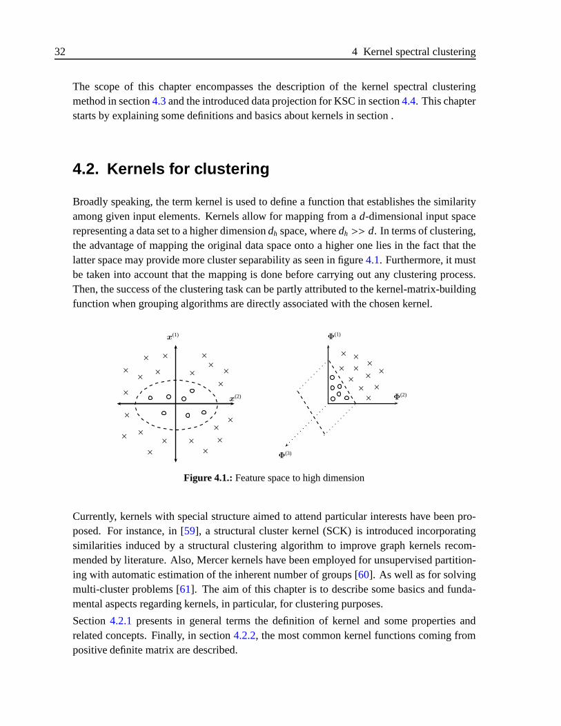
32 4 Kernel spectral clustering
The scope of this chapter encompasses the description of the kernel spectral clusteringmethod in section4.3and the introduced data projection for KSC in section4.4. This chapterstarts by explaining some definitions and basics about kernels in section .
4.2. Kernels for clustering
Broadly speaking, the term kernel is used to define a function that establishes the similarityamong given input elements. Kernels allow for mapping from ad-dimensional input spacerepresenting a data set to a higher dimensiondh space, wheredh >> d. In terms of clustering,the advantage of mapping the original data space onto a higher one lies in the fact that thelatter space may provide more cluster separability as seen in figure4.1. Furthermore, it mustbe taken into account that the mapping is done before carrying out any clustering process.Then, the success of the clustering task can be partly attributed to the kernel-matrix-buildingfunction when grouping algorithms are directly associated with the chosen kernel.
×
×××
××
××
×
×
×
×
×
××
× × ×
×× ××
× ×××
×
×
x(1)
x(2) Φ(2)
Φ(1)
Φ(3)
××
××
Figure 4.1.:Feature space to high dimension
Currently, kernels with special structure aimed to attend particular interests have been pro-posed. For instance, in [59], a structural cluster kernel (SCK) is introduced incorporatingsimilarities induced by a structural clustering algorithm to improve graph kernels recom-mended by literature. Also, Mercer kernels have been employed for unsupervised partition-ing with automatic estimation of the inherent number of groups [60]. As well as for solvingmulti-cluster problems [61]. The aim of this chapter is to describe some basics and funda-mental aspects regarding kernels, in particular, for clustering purposes.
Section4.2.1 presents in general terms the definition of kernel and some properties andrelated concepts. Finally, in section4.2.2, the most common kernel functions coming frompositive definite matrix are described.
4.2 Kernels for clustering 33
4.2.1. Kernel function
In terms of human learning theory [62], one of the fundamental problems is the discrimi-nation among elements or objects. Take the following instance: We have a set of objectsformed by two different classes; then, when a new object appears the task is to determine towhich class such an object belongs. This is usually done by taking into account the object’sproperties as well as similarities and differences with regards to the two previously knownclasses. According to the above, and regarding kernel theory, we need to create or choose asimilarity or affinity measure to compare the data.
Kernels considered in this work are positive definite, and then Gram Matrix (or kernel matrix)must be positive definite as well. In other words, we can define a kernel function in the form
K(·, ·) :Kd × Kd −→ Kxi,x j 7−→ K(xi,x j) (4.1)
whereK = C or R. Note that in this case we have assumed elementsxi to be real andd-dimensional. Then, if we have a total ofN elements or data points, aN × N matrixΩ withentriesΩi j = K(xi,x j) is called Gram matrix or kernel matrix as well. Therefore, the kernelmatrix must be a positive matrix, i.e., aN × N complex matrixΩ satisfying
N∑
i=1
N∑
j=1
ci cjΩi j ≥ 0 (4.2)
for all ci ∈ C is called positive definite, being ¯ci the complex conjugate ofci. Similarly, a realsymmetricN × N matrixK satisfying4.2 for all ci ∈ R is also called positive definite [63].Note that a symmetric matrix is positive if and only if all its eigenvalues are non-negative.In the literature, a number of different terms are used for positive definite kernels, such asreproducing kernel, Mercer kernel, admissible kernel, support vector kernel, non-negativedefinite kernel and covariance function [63]. Now, let us consider a function to map from thed-dimensional space to thatdh dimensional one is in the formφ(·), such that:
φ(·) :Rd −→ Rdh
xi 7−→ φ(xi) (4.3)
The matrixΦ =[φ(x1)⊤, . . . ,φ(xN)⊤
]⊤, Φ ∈ RN×dh, is a high dimensional representation of
the original dataX ∈ RN×d.
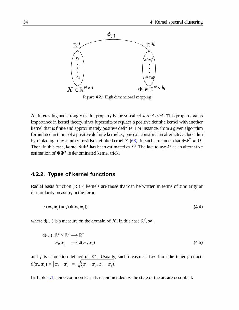
34 4 Kernel spectral clustering
x1
xn
φ(x1)
φ(xn)
φ(·)
Rd R
dh
X ∈ RN×d Φ ∈ RN×dh
Figure 4.2.:High dimensional mapping
An interesting and strongly useful property is the so-calledkernel trick. This property gainsimportance in kernel theory, since it permits to replace a positive definite kernel with anotherkernel that is finite and approximately positive definite. For instance, from a given algorithmformulated in terms of a positive definite kernelK, one can construct an alternative algorithmby replacing it by another positive definite kernelK [63], in such a manner thatΦΦ
T= Ω.
Then, in this case, kernelΦΦT has been estimated asΩ. The fact to useΩ as an alternative
estimation ofΦΦT is denominated kernel trick.
4.2.2. Types of kernel functions
Radial basis function (RBF) kernels are those that can be written in terms of similarity ordissimilarity measure, in the form:
K(xi,x j) = f (d(xi ,x j)), (4.4)
where d(·, ·) is a measure on the domain ofX, in this caseRd, so:
d(·, ·) :Rd × Rd −→ R+
xi,x j 7−→ d(xi ,x j) (4.5)
and f is a function defined onR+. Usually, such measure arises from the inner product;
d(xi,x j) =∥∥∥xi − x j
∥∥∥ =√⟨
xi − x j,xi − x j
⟩.
In Table4.1, some common kernels recommended by the state of the art are described.
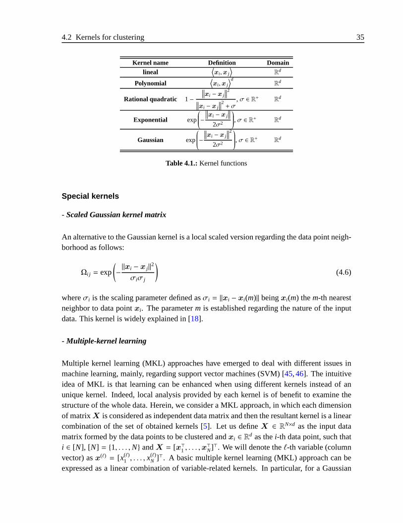
4.2 Kernels for clustering 35
Kernel name Definition Domainlineal
⟨xi ,x j
⟩R
d
Polynomial⟨xi ,x j
⟩dR
d
Rational quadratic 1−∥∥∥xi − x j
∥∥∥2
∥∥∥xi − x j
∥∥∥2+ σ
, σ ∈ R+ Rd
Exponential exp
−∥∥∥xi − x j
∥∥∥2σ2
, σ ∈ R+ Rd
Gaussian exp
−∥∥∥xi − x j
∥∥∥2
2σ2
, σ ∈ R+ Rd
Table 4.1.:Kernel functions
Special kernels
- Scaled Gaussian kernel matrix
An alternative to the Gaussian kernel is a local scaled version regarding the data point neigh-borhood as follows:
Ωi j = exp
(−||xi − x j ||2
σiσ j
)(4.6)
whereσi is the scaling parameter defined asσi = ||xi − xi(m)|| beingxi(m) them-th nearestneighbor to data pointxi. The parameterm is established regarding the nature of the inputdata. This kernel is widely explained in [18].
- Multiple-kernel learning
Multiple kernel learning (MKL) approaches have emerged to deal with different issues inmachine learning, mainly, regarding support vector machines (SVM) [45,46]. The intuitiveidea of MKL is that learning can be enhanced when using different kernels instead of anunique kernel. Indeed, local analysis provided by each kernel is of benefit to examine thestructure of the whole data. Herein, we consider a MKL approach, in which each dimensionof matrixX is considered as independent data matrix and then the resultant kernel is a linearcombination of the set of obtained kernels [5]. Let us defineX ∈ RN×d asthe input datamatrix formed by the data points to be clustered andxi ∈ Rd as thei-th data point, such thati ∈ [N], [N] = 1, . . . ,N andX = [x⊤1 , . . . ,x
⊤N]⊤. We will denote theℓ-th variable (column
vector) asx(ℓ)= [x(ℓ)
1 , . . . , x(ℓ)N ]⊤. A basic multiple kernel learning (MKL) approach can be
expressed as a linear combination of variable-related kernels. In particular, for a Gaussian
36 4 Kernel spectral clustering
kernelΩ ∈ RN×N, we have:
Ω =
d∑
ℓ=1
ρℓΩℓ (4.7)
whereΩℓ is the kernel associated to variableℓ being each entry
Ω(ℓ)i j = exp
−|x(ℓ)
i − x(ℓ)j |2
2σ2
, ∀i, j ∈ [N] (4.8)
andρ = [ρ1, . . . , ρd] is the vector of coefficients. As explained in [5], vectorρ can beestimated under a variable-relevance criterion, for example, a PCA-derived one as follows:
ρ =
d∑
ℓ=1
λℓvℓ vℓ (4.9)
whereλℓ andvℓ are respectively theℓ-th eigenvalue and eigenvector of the covariance matrixof X and stands for the Hadamard (element-wise) product.
4.3. Least-squares SVM formulation for kernelspectral clustering
KSC is aiming to split the input data matrixX ∈ RN×d: X = [x⊤1 , . . . ,x⊤N]⊤, into K disjoint
subsets, wherexi ∈ Rd is thei-th d dimensional data point,N is the number of data point,andK is the number of desired groups. In the following, the clustering mode is described.Let e(l) ∈ RN be thel-th projection vector, which is assumed in the following latent variableform:
e(l)= Φw(l)
+ bl1N (4.10)
wherew(l) ∈ Rdh is thel-th weighting vector,bl is a bias term,ne is the number of consid-ered latent variables, notation1N stands for aN dimensional all-ones vector, and the matrixΦ =
[φ(x1)⊤, . . . ,φ(xN)⊤
]⊤, Φ ∈ RN×dh, is a high dimensional representation of data. The
functionφ(·) maps data from the original dimension to a higher onedh, i.e.,φ(·) : Rd → Rdh.Therefore,e(l) represents the latent variables from a set ofne binary cluster indicators ob-tained with sign(e(l)), which are to be further encoded to obtain theK resultant groups.
Grounded on the least-squares SVM formulation of equation (4.10), the following optimiza-tion problem can be stated:
maxe(l),w(l),b(l)
12N
ne∑
l=1
γle(l)⊤V e(l) − 1
2
ne∑
l=1
w(l)⊤w(l) (4.11a)
s. t. e(l)= Φ
⊤w(l)+ bl1N (4.11b)
4.3 Least-squares SVM formulation for kernel spectral clustering 37
whereγl ∈ R+ is the l-th regularization parameter andV ∈ RN×N is a diagonal matrix repre-senting the weight of projections.
Thinking of further analysis, we express the above primal formulation in matrix terms, asfollows:
maxE,W ,b
12N
tr(E⊤V EΓ ) − 12
tr(W ⊤W ) (4.12a)
s. t. E = ΦW + 1N ⊗ b⊤ (4.12b)
whereb = [b1, . . . , bne], b ∈ Rne, Γ = Diag([γ1, . . . , γne]), W = [w(1), · · · ,w(ne)], W ∈R
dh×ne, andE = [e(1), · · · , e(ne)], E ∈ RN×ne. Notations tr(·) and⊗ denote the trace andthe Kronecker product, respectively. By minimizing the previous cost function, the goalsof minimizing the weighting variance ofE and maximizing the variance ofW are reachedsimultaneously. LetΣE the weighting covariance matrix ofE andΣW the covariance matrixof W . Since matrixV is diagonal, we have that tr((V 1/2E)⊤V 1/2E) = tr(ΣE). In otherwords,ΣE is the covariance matrix of weighted projections, i.e., the projections scaled bysquare root of matrixV . As well, tr(W ⊤W ) = tr(ΣW ). Then, KSC can be seen as aKernel WPCA approach.
4.3.1. Solving the KSC problem
To solve the KSC problem, we form the corresponding Lagrangian of problem from equation(4.11) as follows:
L(E,W ,Γ ,A) =1
2Ntr(ΓE⊤V E) − 1
2tr(W ⊤W )
− tr(A⊤(E −ΦW − 1N ⊗ b⊤)) (4.13)
where matrixA ∈ RN×ne holds the Lagrange multiplier vectorsA = [α(1), · · · ,α(ne)], andα(l) ∈ RN is thel-th vector of Lagrange multipliers.
Solving the partial derivatives onL(E,W ,Γ ,A) to determine the Karush-Kuhn-Tuckerconditions, we obtain:
∂L
∂E= 0 ⇒ E = NV −1AΓ −1
∂L
∂W= 0 ⇒W = Φ
⊤A
∂L
∂A= 0 ⇒ E = ΦW
∂L
∂b= 0 ⇒ b⊤1N = 0
38 4 Kernel spectral clustering
Therefore, by eliminating the primal variables from initial problem (4.11) and assuming akernel trick such thatΦΦ
⊤= Ω, beingΩ ∈ RN×N a given kernel matrix (see chapter4.2),
the following eigenvectors-based dual solution is obtained:
AΛ = AV (IN + (1N ⊗ b⊤)(ΩΛ)−1)Ω (4.14)
whereΛ = Diag(λ),Λ ∈ RN×N, λ ∈ RN is the vector of eigenvalues withλl = N/γl , λl ∈ R+.Also, taking into account that the kernel matrix represents the similarity matrix of a graphwith K connected components as well asV = D−1 whereD ∈ RN×N is the degree matrixdefined asD = Diag(Ω1N); then theK − 1 eigenvectors contained inA, associated tothe largest eigenvalues, are piecewise constant and become indicators of the correspondingconnected parts of the graph. Therefore, valuene is fixed to beK − 1 [55]. With the aim ofachieving a dual formulation, but satisfying the conditionb⊤1N = 0 by centering vectorb(i.e. with zero mean), the bias term should be chosen in the form
bl = −1/(1⊤NV 1N)1⊤NV Ωα(l). (4.15)
Thus, the solution of problem of equation (4.12) is reduced to the following eigenvector-related problem:
AΛ = V HΩA (4.16)
where matrixH ∈ RN×N is the centering matrix that is defined as
H = IN −1
1⊤NV 1N1N1
⊤NV ,
whereIN denotes aN-dimensional identity matrix and,Ω = [Ωi j ], Ω ∈ RN×N, beingΩi j =
K(xi,x j), i, j ∈ [N]. NotationK(·, ·) : Rd × Rd → R stands for the kernel function. As aresult, the set of projections can be calculated as follows:
E = ΩA + 1N ⊗ b⊤ (4.17)
Once projections are calculated, we proceed to carry out the cluster assignment by follow-ing an encoding procedure applied on projections. Because each cluster is represented by asingle point in theK − 1-dimensional eigenspace, such that those single points are always indifferent orthants due also to the KKT conditions, we can encode the eigenvectors consider-ing that two points are in the same cluster if they are in the same orthant in the correspondingeigenspace [55]. Then, a code book can be obtained from the rows of the matrix containingthe K − 1 binarized leading eigenvectors in the columns, by using sign(e(l)). Then, matrixE = sgn(E) is the code book being each row a codeword.
4.4 Proposed data projection for KSC 39
4.3.2. Out-of-sample extension
KSC can be extended to out-of-samples analysis without re-clustering the whole data to de-termine the assignment cluster membership for new testing data [55]. In particular, definingz ∈ Rne asthe projection vector of a testing data pointxtest, and by taking into considerationthe training clustering model, the testing projections can be computed as:
z = A⊤Ωtest+ b (4.18)
whereΩtest ∈ Rne is the kernel vector such that
Ωtest= [Ωtest1, . . . , ΩtestN ]⊤,
whereΩtesti = K(xi,xtest). Once, the test projection vectorz is computed, a decoding stageis carried out that consists of comparing the binarized projections with respect to the code-words in the code bookE and assigning cluster membership based on the minimal Hammingdistance [55].
4.3.3. KSC algorithm
Following the pseudo-code (Algorithm3) to perform KSC is shown.
Algorithm 3 Kernel spectral clustering: [qtrain, qtest] = KSC(X ,K(·, ·),K)
1: Input: K, X, K(·, ·)
2: Form the kernel matrix Ω such that Ωi j = K(yi ,x j)3: Determine E through (4.17)4: Form the training codebook by binarizing E = sgn(E)5: Assign the output training labels qtrain according to similar codewords
6: Compute the training codewords for testing
7: Assign the output testing labels qtest according to the minimal Hamming distance when
comparing with training codewords
8: Output: qtrain, qtest
4.4. Proposed data projection for KSC
In some pattern recognition problems when data are represented in a significantly high di-mensional space or have redundant information, feature extraction and selection process takeplace as an essential stage for designing a clustering scheme. The problem of analyzing anddetermining the relevance of features or attributes representing a data set is typical in the pat-tern recognition and learning machine fields. It is often necessary in different science fields:
40 4 Kernel spectral clustering
word processing,bio-informatics, among others. In [64], a relevance concept is presented,which is based on the Laplacian spectral properties of the affinity matrix using either su-pervised and unsupervised inferences. The feature selection process is performed trough aniterative optimization method based on least squares. This method is calledQ−α, beingQ arotation matrix andα a weighting vector. In another work [65], authors apply theQ−α witha power embedded algorithm. Another works, [66–68] combine feature selection approacheswith dimensionality reduction so that the relevance vectors are used as weighting factors areto carry a process of weighted principal component analysis (WPCA). Also, [67] presents ascheme based on a generalized distance allowing to express several WPCA approaches forfeature extraction purposes according to a similarity matrix.
In the following, we introduce a data projection for improving the KSC performance. Dataprojection transforms data from the originald-dimensional feature space into a reducedp-dimensional one. However, since the cluster structure is the most important characteristicdescribing the input data, the main goal of data projection is to find a lower dimensionalityrepresentation maximally preserving the original cluster structure. Herein, we introduce adata projection that focus on the analyzes of the local data structure to improve the KSCclustering method. Specifically, we propose the dimension reduction based on the M-innerproduct approach, in which the similarity between data points is considered, as describedin [68] for clustering purposes. Proposed scheme improves the performance of kernel spec-tral clustering since, firstly, the data global structure is taken into account in the projectionprocess and, secondly, kernel method exploit the local structures information.
Proposed data projection is summarized as follows: Given both an input data matrixX ,
as well as any orthonormal rotation matrixQ ∈ Rd×d, such thatQTQ = Id; then, we canintroduce a lineal data projection, as
Y =XQ,
whereY ∈ RN×d. To accomplish the dimensionality reduction, we consider the reducedrotation matrixQ ∈ Rd×p, that is a truncated representation ofQ, wherep < d and satisfies anothonormal condition:QTQ = Ip. Likewise, a truncated linearly projected dataY ∈ RN×p isintroduced, such thatY =XQ. Consequently, we can yield an expression for reconstructeddata matrixX = Y Q⊤, X ∈ RN×d. SinceQ is p-dimensional,X becomes a lower rankmatrix representing the original dataX.
In order to obtain a rotation matrixQ, such thatY holds the projected vectors mostly con-tributing to the explained variance regarding matrixΣ, and using theM-inner norm as adistance measure to quantify the quality of provided data projection, it is possible to device
4.4 Proposed data projection for KSC 41
the following optimization problem:
minQ
||X − X ||2Σ = maxQ
tr(Q⊤X⊤ΣXQ) (4.19a)
s. t. Q⊤Q = Id (4.19b)
where||X ||2Σ
denotes the squaredM-norm ofX regarding any positive semi-definite matrixΣ, such that||X ||2
Σ= tr(X⊤ΣX).
Formulation given by equation (4.19a) takes place, since we can verify the following identity[68]:
||X ||2Σ = ||X − X ||2Σ + tr(Q⊤X⊤ΣXQ)
This is widely explained in appendixD. Then, because||X ||2Σ
remains constant, the aim ofminimizing ||X − X ||2
Σas well as maximizing tr(Q⊤X⊤ΣXQ) can be reached simulta-
neously. Furthermore, to incorporate the information given by the assumed similarity intothe data projection process, we employ the kernel matrixΩ as positive semidefinite matrix,i.e.,Σ = Ω. By considering the maximization problem in equation (4.19a), we can write itsLagrangian, as follows:
L(Q,∆) = tr(X⊤ΩX) − tr(∆⊤(Q⊤Q − Id))
Then, equating the partial derivatives in the form:
∂
∂Qtr(Q⊤X⊤ΩXQ) =
∂
∂Qtr(∆⊤(Q⊤Q − Id)),
we can pose the following eigenvector-related problem:
X⊤ΩXQ = Q∆ (4.20)
where∆ = Diag(δ), ∆ ∈ Rd×d, and vectorδ = [δ1, . . . , δd] holds the Lagrangian mul-tipliers. From Equation (4.20), we can infer that a feasible solution of this problem canbeaccomplished by selecting the Lagrange multipliers as the eigenvalues and matrixQ asthe longestp eigenvectors ofX⊤ΩX . Dimensionp can be established by means of well-known explained variance criterion. Finally, the output projected data can be computed asY =XQ. Assumingyi as thei-th row vector ofY , the projections for training data are:
E = ΩA + 1N ⊗ b⊤ (4.21)
whereΩ = [Ωi j ] andΩi j = K(yi , y j).
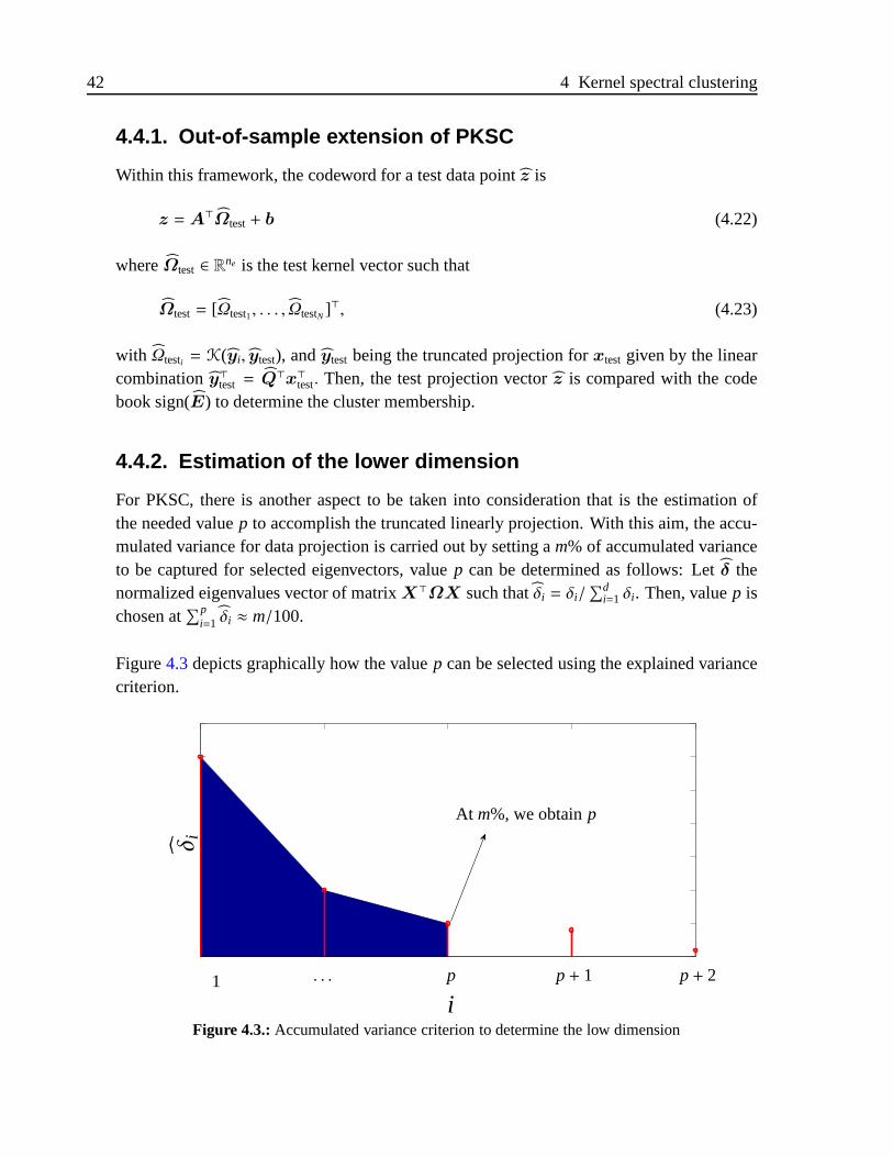
42 4 Kernel spectral clustering
4.4.1. Out-of-sample extension of PKSC
Within this framework, the codeword for a test data pointz is
z = A⊤Ωtest+ b (4.22)
whereΩtest ∈ Rne is the test kernel vector such that
Ωtest= [Ωtest1, . . . , ΩtestN ]⊤, (4.23)
with Ωtesti = K(yi, ytest), andytest being the truncated projection forxtest given by the linearcombinationy⊤test = Q⊤x⊤test. Then, the test projection vectorz is compared with the codebook sign(E) to determine the cluster membership.
4.4.2. Estimation of the lower dimension
For PKSC, there is another aspect to be taken into consideration that is the estimation ofthe needed valuep to accomplish the truncated linearly projection. With this aim, the accu-mulated variance for data projection is carried out by setting am% of accumulated varianceto be captured for selected eigenvectors, valuep can be determined as follows: Letδ thenormalized eigenvalues vector of matrixX⊤ΩX such thatδi = δi/
∑di=1 δi. Then, valuep is
chosen at∑p
i=1 δi ≈ m/100.
Figure4.3depicts graphically how the valuep can be selected using the explained variancecriterion.
At m%, we obtainp
δi
ip1 p+ 1 p+ 2. . .
Figure 4.3.:Accumulated variance criterion to determine the low dimension

4.4 Proposed data projection for KSC 43
4.4.3. PKSC algorithm
Algorithm4 summarizes the steps for PKSC.
Algorithm 4 Projected KSC: [ ˆqtrain, qtest] = PKSC(X ,K(·, ·),K, p)
1: Input: K, X, K(·, ·), p
2: Compute Q as the eigenvectors associated with the largest p eigenvalues of X⊤ΩX, being
Ωi j = K(xi ,x j).3: Compute Y =XQ.
4: Form the kernel matrix Ω with entries Ωi j = K(yi , y j)5: Apply KSC over Y : [qtrain, qtest] = KSC(X ,K(·, ·),K) (see Algorithm 3)
6: Output: qtrain, qtest
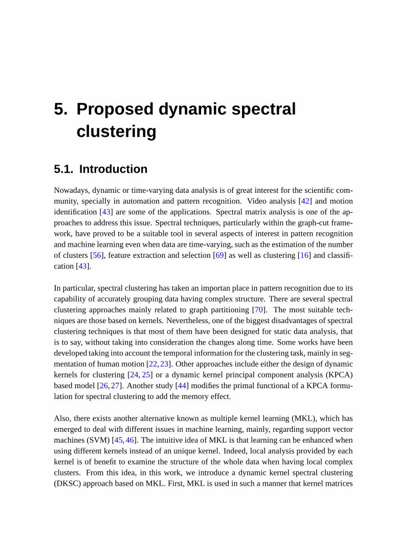
5. Proposed dynamic spectralclustering
5.1. Introduction
Nowadays, dynamic or time-varying data analysis is of great interest for the scientific com-munity, specially in automation and pattern recognition. Video analysis [42] and motionidentification [43] are some of the applications. Spectral matrix analysis is oneof the ap-proaches to address this issue. Spectral techniques, particularly within the graph-cut frame-work, have proved to be a suitable tool in several aspects of interest in pattern recognitionand machine learning even when data are time-varying, such as the estimation of the numberof clusters [56], feature extraction and selection [69] as well as clustering [16] and classifi-cation [43].
In particular, spectral clustering has taken an importan place in pattern recognition due to itscapability of accurately grouping data having complex structure. There are several spectralclustering approaches mainly related to graph partitioning [70]. The most suitable tech-niques are those based on kernels. Nevertheless, one of the biggest disadvantages of spectralclustering techniques is that most of them have been designed for static data analysis, thatis to say, without taking into consideration the changes along time. Some works have beendeveloped taking into account the temporal information for the clustering task, mainly in seg-mentation of human motion [22,23]. Other approaches include either the design of dynamickernels for clustering [24, 25] or a dynamic kernel principal component analysis (KPCA)based model [26,27]. Another study [44] modifies the primal functional of a KPCA formu-lation for spectral clustering to add the memory effect.
Also, there exists another alternative known as multiple kernel learning (MKL), which hasemerged to deal with different issues in machine learning, mainly, regarding support vectormachines (SVM) [45,46]. The intuitive idea of MKL is that learning can be enhanced whenusing different kernels instead of an unique kernel. Indeed, local analysis provided by eachkernel is of benefit to examine the structure of the whole data when having local complexclusters. From this idea, in this work, we introduce a dynamic kernel spectral clustering(DKSC) approach based on MKL. First, MKL is used in such a manner that kernel matrices
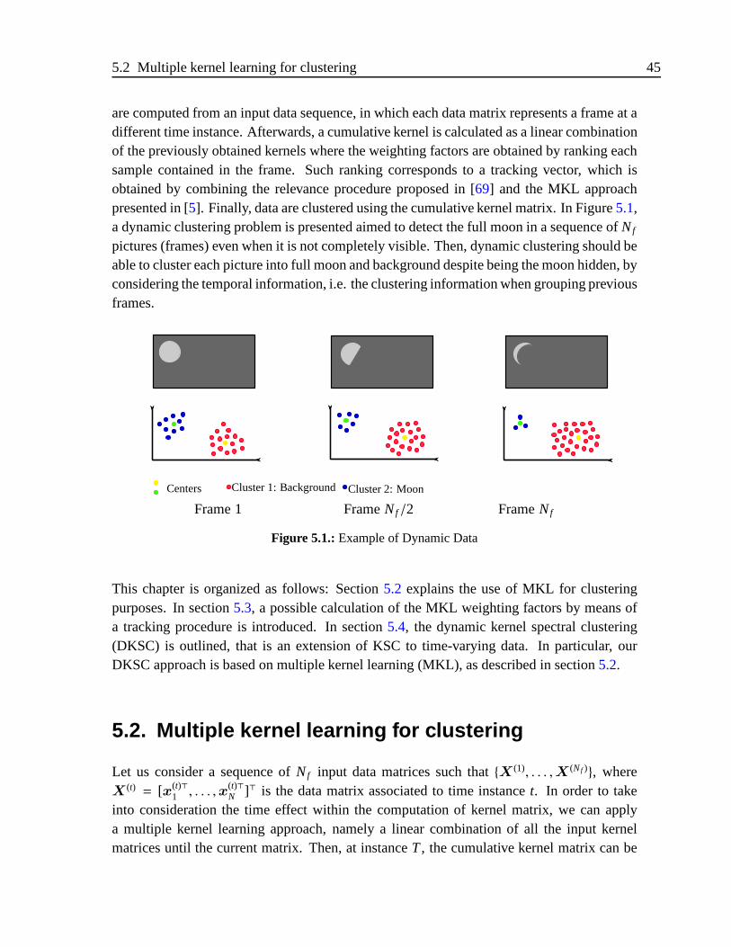
5.2 Multiple kernel learning for clustering 45
are computed from an input data sequence, in which each data matrix represents a frame at adifferent time instance. Afterwards, a cumulative kernel is calculated as a linear combinationof the previously obtained kernels where the weighting factors are obtained by ranking eachsample contained in the frame. Such ranking corresponds to a tracking vector, which isobtained by combining the relevance procedure proposed in [69] and the MKL approachpresented in [5]. Finally, data are clustered using the cumulative kernel matrix. In Figure5.1,a dynamic clustering problem is presented aimed to detect the full moon in a sequence ofNf
pictures (frames) even when it is not completely visible. Then, dynamic clustering should beable to cluster each picture into full moon and background despite being the moon hidden, byconsidering the temporal information, i.e. the clustering information when grouping previousframes.
Centers Cluster 1: Background Cluster 2: Moon
Frame 1 FrameNf /2 FrameNf
Figure 5.1.:Example of Dynamic Data
This chapter is organized as follows: Section5.2 explains the use of MKL for clusteringpurposes. In section5.3, a possible calculation of the MKL weighting factors by means ofa tracking procedure is introduced. In section5.4, the dynamic kernel spectral clustering(DKSC) is outlined, that is an extension of KSC to time-varying data. In particular, ourDKSC approach is based on multiple kernel learning (MKL), as described in section5.2.
5.2. Multiple kernel learning for clustering
Let us consider a sequence ofNf input data matrices such thatX (1), . . . ,X (Nf ), whereX (t)
= [x(t)⊤1 , . . . ,x
(t)⊤N ]⊤ is the data matrix associated to time instancet. In order to take
into consideration the time effect within the computation of kernel matrix, we can applya multiple kernel learning approach, namely a linear combination of all the input kernelmatrices until the current matrix. Then, at instanceT, the cumulative kernel matrix can be
46 5 Proposed dynamic spectral clustering
computed as:
Ω(T)=
T∑
t=1
ηtΩ(t) (5.1)
whereη = [η1, . . . , ηT ] are the weighting factors or coefficients andΩ(t) is the kernel matrixassociated toX (t) such thatΩ(t)
i j = K(x(t)i ,x
(t)j ). Sinceηt is the weighting factor associated to
the data matrix at time instancet within a sequence,η can be seen as a tracking vector. InFigure5.2, the example of moving moon is recalled to graphically explained how the MKLworks for clustering purposes. Each frame is represented by a feature space (data matrix)X (t) which is mapped to a high-dimensional spaceΦ
(t). Then, the corresponding kernelsΩare calculated. Finally, the cumulative kernel matrixΩ is obtained by a linear combination ofpreviously determined kernels. Coefficients or weighting factors for such linear combinationare preset or calculated regarding each frame.
Background Moon
X (1) X (t) X (T)
x(1)
x(2)
x(1)
x(2)
x(1)
x(2)
Φ(1)Φ(1)
Φ(2)
Φ(1)
Φ(2)
Φ(1)
Φ(2)
Φ(t) Φ(T)
η1Ω(1) ηtΩ
(t) ηTΩ(T)· · · + · · · · · · + · · · = Ω(T)
Figure 5.2.:Graphic explanation of MKL for clustering considering the example of changing moon
Cumulative kernel matrices can also be calculated in a recursive fashion by applying
Ω(T)= Ω
(T−1)+ ηTΩ
(T) (5.2)
with Ω(0)= 0N×N.
5.3. Tracking by KSC
The KSC-based tracking (KSCT) approach proposed here arises from the combination ofKSC with a relevance ranking for feature selection introduced in [69]. Such ranking comesfrom a definition of feature relevance aimed to selecting a subset of features founded on
5.3 Tracking by KSC 47
spectral properties of the Laplacian of the data matrix, whichis based on a continuous rank-ing of the features by means of a least-squares maximization problem. The maximizationis done over a functional such that sparse solutions for the ranking values are obtained by aspectral decomposition of a non-negative matrix [69]. What makes this approach interest-ing within the context of dynamic data analysis is the possibility to get a ranking value foreach frame in the process of time-varying data analysis. In addition, such feature relevanceapproach measures the relevance of a subset of features against its influence on the clusterassignment. KSCT is aimed to track moving samples or frames matching each frame to anunique meaningful value. This approach may be of helpfulness because of its unsupervisednature, since, in practice, labeling is often not available for motion tracking applications.
Proposed approach works as follows: It starts by clustering the input data by means of KSCwith a manually established number of groups and a determined kernel function. Then, welinearly project the high dimensional representation of input data in order to apply a samplerelevance ranking process as proposed in [69]. The projection matrix is obtained as a sparsesolution of a quadratic optimization problem, where an energy (also called variance) term ismaximized. It is proved that projection matrix is the same as the eigenvector matrix givenby KSC. Finally, a tracking vector is obtained by a linear combination of such eigenvectorsin a similar way as that described in [5].
5.3.1. Tracking vector
Similarly as the relevance analysis explained in [69] in which a functional regarding anon-negative matrix is introduced, we pose an optimization problem with the differencethat our focus is obtaining the ranking values for samples instead of features, as follows:Consider a data matrix sequenceX (1), . . . ,X (Nf ), whereNf is the number of frames andX (t)= [x(t)⊤
1 , . . . ,x(t)⊤N ]⊤ is the data matrix associated to time instancet in sizeN × d. Also,
consider the frame matrixX ∈ RNf×Nd which is formed in such a way that each row is aframe by letting ˜xt ∈ RNd be the vectorization of coordinates representing thet-th frame.In other words,X = [x⊤1 , . . . , x
⊤Nf
]⊤ and xt = vec(X (t)). The corresponding kernel matrix
can be expressed asΩ ∈ RNf ×Nf such thatΩi j = K(xi , x j). Then, the high dimensionalrepresentation matrixΦ ∈ RNf×dh is
Φ =
[φ(x1)
⊤, . . . ,φ(xNf )⊤]⊤,
whereφ(·) : RNd → Rdh. Assume a linear projection in the formZ = Φ⊤U , whereU is
an orthonormal matrix in sizeNf × Nf . Also, a lower rank representation ofZ is assumedin the formZ = Φ
⊤U , whereU is in sizeNf × c (c < Nf ). Then, an energy maximization
48 5 Proposed dynamic spectral clustering
problem can be written as:
maxU
tr(U⊤ΩU ) (5.3a)
s. t. U⊤U = Ic (5.3b)
Indeed, by using the kernel trick, we have
tr(Z⊤Z) = tr(U⊤ΦΦ⊤U ) = tr(U⊤ΩU ),
Recalling the KSC dual problem explained in chapter4 (specifically equation4.16), we canwrite the centering matrix for frame matrixX, so:
H = INf −1
1⊤NfV 1Nf
1Nf 1⊤NfV ,
whereV is chosen as the degree matrix given byD = Diag(Ω1Nf ).
Then, normalizing regarding degree and centering bothZ and Z, which means to pre-multiply Φ by LV −1/2, we can infer that
tr(U⊤ΩU ) =c∑
t=1
λt
whereL comes from the Cholesky decomposition ofH such thatL⊤L = H andλl is thel-th eigenvalue obtained by KSC when applied overX with a determined number of clustersK, as described in chapter4. Therefore, a feasible solution of the problem isU = A, beingA = [α(1), . . . , α(c)] the corresponding eigenvector matrix. Thus,c is the same number ofconsidered support vectors ˜ne.
Similarly as the MKL approach explained in [5], we introduce a tracking vectorη ∈ RNf asthe solution of minimizing the dissimilarity term given by
‖Φ − Φ‖2F (5.4)
subject to some orthogonality conditions, beingΦ a lower-rank representation ofΦ. Then,the ranking vector can be calculated by:
η =
ne∑
ℓ=1
λℓα(ℓ) α(ℓ) (5.5)
where denotes Hadamard (element-wise) product. Accordingly, the ranking factorηi is asingle value representing an unique frame in a sequence. Notation ˜a means that variablea is
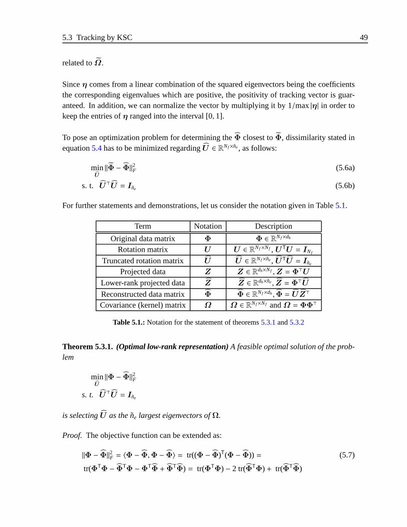
5.3 Tracking by KSC 49
related toΩ.
Sinceη comes from a linear combination of the squared eigenvectors being the coefficientsthe corresponding eigenvalues which are positive, the positivity of tracking vector is guar-anteed. In addition, we can normalize the vector by multiplying it by 1/max|η| in order tokeep the entries ofη ranged into the interval [0,1].
To pose an optimization problem for determining theΦ closest toΦ, dissimilarity stated inequation5.4has to be minimized regardingU ∈ RNf×ne, as follows:
minU
‖Φ − Φ‖2F (5.6a)
s. t. U⊤U = Ine (5.6b)
For further statements and demonstrations, let us consider the notation given in Table5.1.
Term Notation Description
Original data matrix Φ Φ ∈ RNf×dh
Rotation matrix U U ∈ RNf ×Nf , UTU = INf
Truncated rotation matrix U U ∈ RNf×ne, UTU = Ine
Projected data Z Z ∈ Rdh×Nf ,Z = Φ⊤U
Lower-rank projected data Z Z ∈ Rdh×ne, Z = Φ⊤U
Reconstructed data matrix Φ Φ ∈ RNf ×dh, Φ = UZ⊤
Covariance (kernel) matrix Ω Ω ∈ RNf×Nf and Ω = ΦΦ⊤
Table 5.1.:Notation for the statement of theorems5.3.1and5.3.2
Theorem 5.3.1.(Optimal low-rank representation) A feasible optimal solution of the prob-lem
minU
‖Φ − Φ‖2F
s. t. U⊤U = Ine
is selectingU as thene largest eigenvectors ofΩ.
Proof. The objective function can be extended as:
||Φ − Φ||2F = 〈Φ − Φ,Φ − Φ〉 = tr((Φ − Φ)T(Φ − Φ)) = (5.7)
tr(ΦTΦ − ΦT
Φ −ΦTΦ + Φ
TΦ) = tr(ΦT
Φ) − 2 tr(ΦTΦ) + tr(ΦT
Φ)
50 5 Proposed dynamic spectral clustering
Also, trace satisfies the duality
tr(ΦTΦ) − 2 tr(ΦT
Φ) + tr(ΦTΦ) = tr(ΦΦ
T) − 2 tr(ΦΦT) + tr(ΦΦ
T)
Another term of interest is||Φ||2F =∑Nf
l=1 γtλt whereλt andu(t) represent respectively thet–th eigenvalue and eigenvector ofΦΦ
T and γt = λ−1t u(t)T
ΦTΦu(t). Then, re-arranging
equation5.7, we have:
||Φ − Φ||2F =Nf∑
t=1
γtλt − 2ne∑
t=1
γtλt +
ne∑
t=1
γtλt =
Nf∑
t=ne+1
γtλt (5.8)
Therefore, we can notice that there exists a direct relationship between||Φ||2F and equation5.8that can be expressed as:
||Φ||2F =ne∑
t=1
γtλt + ||Φ − Φ||2F = tr(ΦΦT) + ||Φ − Φ||2F .
Since||Φ||2A
is constant, the problem of minimizing||Φ− Φ||2F can be expressed as maximiz-ing its complement tr(ΦΦ
T).
In addition,
tr(ΦΦT) = tr(UZ⊤Φ⊤) = tr(UU⊤ΦΦ
⊤) = tr(U⊤ΦΦ⊤U ).
and, thus, the new optimization problem becomes:
maxU
tr(UTΩU ) (5.9a)
s. t. U⊤U = Ine (5.9b)
To solve the previous problem, we can write a Lagrangian in the form:
L(U |Ω) = f (U |Ω) +ne∑
t=1
λtgt(U ) = tr(UTΩU ) − tr(Λ(U⊤U − Ine)
)
whereΛ = Diag(λ1, . . . , λne) are the Lagrange multipliers.
By solving the first order condition
∂
∂U
(f (U |Ω)
)=
∂
∂U
ne∑
t=1
λtgt(U )
,
wehave that
ΩU = UΛ⇒ U⊤ΩU = Λ

5.3 Tracking by KSC 51
Then, a feasible solution is whenΛ and U are the eigenvalue and eigenvector matrix, re-spectively. Furthermore, since this is a maximization problem, ˜ne largest eigenvectors mustbe selected.
Theorem 5.3.2.(Ranking vector) LetΛ = Diag(λ1, . . . , λNf ) andU = [u(1), . . . ,u(Nf )] theeigen-decomposition ofΩ = ΦΦ
⊤. The ranking of how much contribute each dimensionof Φ⊤ to minimize‖Φ − Φ‖2F when considering ane–dimensional orthonormal base can becalculated as:
η =
ne∑
ℓ=1
λℓu(ℓ) u(ℓ), (5.10)
beingη = [η1, . . . , ηNf ]⊤ andηi the rank value forφi.
Proof. Let us consider the singular value decomposition
Φ = USV⊤ =
Nf∑
t=1
stu(t)v(t)⊤ (5.11)
andφℓ ∈ Rdh be theℓ-th row ofΦ. Then,V = [v(1) · · ·v(dh)] ∈ Rdh×dh are the eigenvectors ofΦ⊤Φ as well asU = [u(1) · · ·u(Nf )] ∈ RNf ×Nf are the eigenvectors ofΩ. MatrixS ∈ RNf ×dh is
formed by the singular valuess1, . . . , sNf . Eigenvectors must be normalized in such a waythat‖u(t)‖ = 1 and‖v(ℓ)‖ = 1 for all ℓ ∈ 1, . . . , dh andt ∈ 1, . . . ,Nf in order to guaranteethat the base becomes orthonormal.
Consider any vectorφt and its lower-rank representationφt, which can be expressed as linearcombinations as follows:
φt =
dh∑
ℓ=1
cℓtv(ℓ)
and
φt =
ne∑
ℓ=1
cℓtv(ℓ),
wherecℓt is theℓ-th coefficient associated tot-th row andne < Nf < dh.
Afterwards, since
‖φt − φt‖2F = 〈φt − φt,φt − φt〉 =
dh∑
ℓ=ne+1
cℓtv(ℓ)
⊤ dh∑
ℓ=ne+1
cℓtv(ℓ)
=
dh∑
ℓ=ne+1
c2ℓtv
(ℓ)⊤v(ℓ)=
dh∑
ℓ=ne+1
c2ℓt
52 5 Proposed dynamic spectral clustering
and
‖φt‖2F =dh∑
ℓ=1
c2ℓt = ‖φt − φt‖2F +
ne∑
ℓ=1
c2ℓt,
minimizing‖φℓ − φℓ‖2F is the same as maximizing∑ne
t=1 c2ℓt.
Then, recalling equation5.11, we have that
tr(U⊤ΩU ) =ne∑
t=1
dh∑
ℓ=1
c2ℓt =
ne∑
t=1
s2t tr(u(t)u(t)⊤) =
ne∑
t=1
λtu(t)⊤u(t)
=
ne∑
t=1
λt.
Thus, we can infer that the contribution ofφt to either maximize the quadratic form tr(U⊤ΩU )or minimize‖Φ − Φ‖2F is given by
ηt =
ne∑
ℓ=1
s2ℓ(u
(ℓ)t )
2=
ne∑
ℓ=1
λℓ(u(ℓ)t )2
whereu(ℓ)t is the entryt of vectoru(ℓ).
Finally, for all theNf dimensions, the ranking vector is then
η =
ne∑
ℓ=1
λℓu(ℓ) u(ℓ)
=
ne∑
ℓ=1
λℓα(ℓ) α(ℓ), (5.12)
This can also be inferred from the energy termΦΦ⊤ that, according to equation5.11, can be
written as:
ΦΦ⊤= USV⊤VS⊤U⊤ = USS⊤U⊤
And, tr(USS⊤U⊤) = tr(UΛU⊤).
5.3.2. KSC-based tracking algorithm
The steps for calculating the proposed KSC-based tracking (KSCT) vectors are summarizedin Algorithm 5.
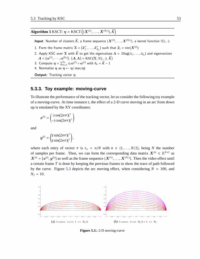
5.3 Tracking by KSC 53
Algorithm 5 KSCT: η = KSCT(X (1), . . . ,X (Nf ), K
)
Input: Number of clusters K, a frame sequence X (1), . . . ,X (Nf ), a kernel function K(·, ·)
1. Form the frame matrix X = [x⊤1 , . . . , x⊤Nf
] such that xt = vec(X (t))
2. Apply KSC over X with K to get the eigenvalues Λ = Diag(λ1, . . . , λne) and eigenvectors
A = [α(1), · · · ,α(ne)]: [A,Λ] = KSC(X,K(·, ·), K)
3. Compute η =∑neℓ=1 λℓα
(ℓ) α(ℓ) with ne = K − 14. Normalize η as η ← η/max|η|
Output: Tracking vector η
5.3.3. Toy example: moving-curve
To illustrate the performance of the tracking vector, let us consider the following toy exampleof a moving-curve. At time instancet, the effect of a 2-D curve moving in an arc from downup is emulated by the XY coordinates:
x(t)=
(| cos(2πτ )|⊤−| cos(2πτ )|⊤
)
and
y(t)=
(|t sin(2πτ )|⊤|t sin(2πτ )|⊤
),
where each entry of vectorτ is τn = n/N with n ∈ 1, . . . ,N/2, being N the numberof samples per frame. Then, we can form the corresponding data matrixX (t) ∈ RN×2 asX (t)= [x(t),y(t)] as well as the frame sequenceX (1), . . . ,X (Nf ). Then the video effect until
a certain frameT is done by keeping the previous frames to show the trace of path followedby the curve. Figure5.3 depicts the arc moving effect, when consideringN = 100, andNf = 10.
−1 −0.8 −0.6 −0.4 −0.2 0 0.2 0.4 0.6 0.8 1
−0.2
0
0.2
0.4
0.6
0.8
1
1.2
(a) Frames from 1 to Nf /2
−1 −0.8 −0.6 −0.4 −0.2 0 0.2 0.4 0.6 0.8 1
−0.2
0
0.2
0.4
0.6
0.8
1
1.2
(b) Frames from Nf /2+ 1 to Nf
Figure 5.3.:2-D moving-curve

54 5 Proposed dynamic spectral clustering
The clustering is done by using KSC aimed to identify two natural movements or clusters(K = 2). To carried out the clustering, KSC is used with a scaled Gaussian kernelK(·, ·)by selecting the 7th (m = 7) nearest neighbor as scaling parameter, as explained in chapter4.2 (section4.2.2). The whole frame matrix is used for training, then ˜qtrain are the clusterassignment to color the frames according to the found groups, being
qtrain = KSC(X,K(·, ·), K). (5.13)
To add noise to the moving-curve model, we consider an additive noise to be applied overthe Y coordinate in the formνn, whereν is the noise level andn ∈ RN is the introduced noisefollowing a Gaussian distributionn ∼ N(0, 1), so:
y(t)n= y + νn. (5.14)
Some examples of the tracking performance are shown in figures5.4 and5.5 when settingthe number of frames to beNf = 100 and the number of samples per frame to beN = 100,representing two experiments changing the number of groups and noise conditions. Fig-ure5.4shows the behavior of tracking vector for clustering the framematrix into 3 clusters(K = 3) while Figure5.5 is for K = 4.
Tracking vector is calculated in both noisy and non-noisy environments by varying the noiselevelν, by assuming that the frame matrixX is to be split intoK clusters. In both figures, foreach considered level noise, clustered sequence at time instancet is shown on the top row aswell as the behavior of the corresponding vector plotting on the bottom row.
To assess the robustness of this approach, we assess the tracking vector over the noise levelsν ∈ 0.05, 0.1. No noise case is also considered (ν = 0). For visualization, purposes somemeaningful frames from the two experiments are selected. For the first experiments, selectedframes aret ∈ 31, 71, 100. Likewise, framest ∈ 31, 50, 75, 100are selected for the secondexperiment.
Also, in order to observe the behavior of tracking vector between clusters, frame matrices areclustered with KSC as shown in equation5.13by considering the same conditions mentionedabove. As it can be appreciated, the shape of the tracking vector has inflections on thetransition from a cluster to the next one. Then, the vector plotting is directly related to thethe changes along the frame sequence. In addition, since there are no changes in the trackingvector when adding noise, it is possible to say that is less sensitive to noisy input data.
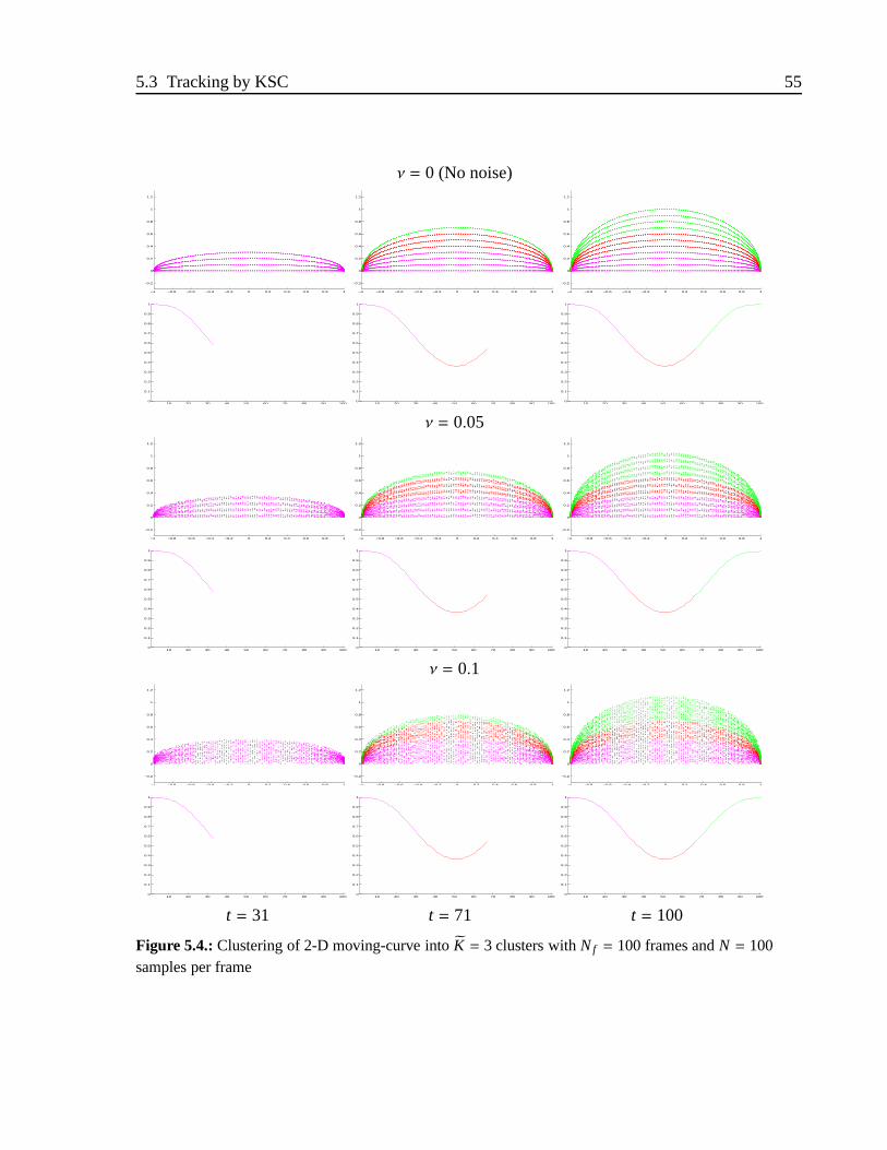
5.3 Tracking by KSC 55
ν = 0 (No noise)
−1 −0.8 −0.6 −0.4 −0.2 0 0.2 0.4 0.6 0.8 1
−0.2
0
0.2
0.4
0.6
0.8
1
1.2
−1 −0.8 −0.6 −0.4 −0.2 0 0.2 0.4 0.6 0.8 1
−0.2
0
0.2
0.4
0.6
0.8
1
1.2
−1 −0.8 −0.6 −0.4 −0.2 0 0.2 0.4 0.6 0.8 1
−0.2
0
0.2
0.4
0.6
0.8
1
1.2
10 20 30 40 50 60 70 80 90 1000
0.1
0.2
0.3
0.4
0.5
0.6
0.7
0.8
0.9
1
10 20 30 40 50 60 70 80 90 1000
0.1
0.2
0.3
0.4
0.5
0.6
0.7
0.8
0.9
1
10 20 30 40 50 60 70 80 90 1000
0.1
0.2
0.3
0.4
0.5
0.6
0.7
0.8
0.9
1
ν = 0.05
−1 −0.8 −0.6 −0.4 −0.2 0 0.2 0.4 0.6 0.8 1
−0.2
0
0.2
0.4
0.6
0.8
1
1.2
−1 −0.8 −0.6 −0.4 −0.2 0 0.2 0.4 0.6 0.8 1
−0.2
0
0.2
0.4
0.6
0.8
1
1.2
−1 −0.8 −0.6 −0.4 −0.2 0 0.2 0.4 0.6 0.8 1
−0.2
0
0.2
0.4
0.6
0.8
1
1.2
10 20 30 40 50 60 70 80 90 1000
0.1
0.2
0.3
0.4
0.5
0.6
0.7
0.8
0.9
1
10 20 30 40 50 60 70 80 90 1000
0.1
0.2
0.3
0.4
0.5
0.6
0.7
0.8
0.9
1
10 20 30 40 50 60 70 80 90 1000
0.1
0.2
0.3
0.4
0.5
0.6
0.7
0.8
0.9
1
ν = 0.1
−1 −0.8 −0.6 −0.4 −0.2 0 0.2 0.4 0.6 0.8 1
−0.2
0
0.2
0.4
0.6
0.8
1
1.2
−1 −0.8 −0.6 −0.4 −0.2 0 0.2 0.4 0.6 0.8 1
−0.2
0
0.2
0.4
0.6
0.8
1
1.2
−1 −0.8 −0.6 −0.4 −0.2 0 0.2 0.4 0.6 0.8 1
−0.2
0
0.2
0.4
0.6
0.8
1
1.2
10 20 30 40 50 60 70 80 90 1000
0.1
0.2
0.3
0.4
0.5
0.6
0.7
0.8
0.9
1
10 20 30 40 50 60 70 80 90 1000
0.1
0.2
0.3
0.4
0.5
0.6
0.7
0.8
0.9
1
10 20 30 40 50 60 70 80 90 1000
0.1
0.2
0.3
0.4
0.5
0.6
0.7
0.8
0.9
1
t = 31 t = 71 t = 100
Figure 5.4.:Clustering of 2-D moving-curve intoK = 3 clusters withNf = 100 frames andN = 100samples per frame
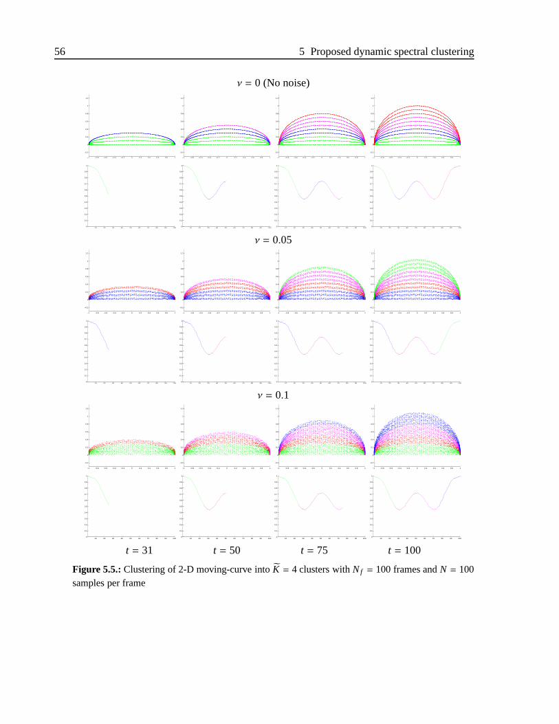
56 5 Proposed dynamic spectral clustering
ν = 0 (No noise)
−1 −0.8 −0.6 −0.4 −0.2 0 0.2 0.4 0.6 0.8 1
−0.2
0
0.2
0.4
0.6
0.8
1
1.2
−1 −0.8 −0.6 −0.4 −0.2 0 0.2 0.4 0.6 0.8 1
−0.2
0
0.2
0.4
0.6
0.8
1
1.2
−1 −0.8 −0.6 −0.4 −0.2 0 0.2 0.4 0.6 0.8 1
−0.2
0
0.2
0.4
0.6
0.8
1
1.2
−1 −0.8 −0.6 −0.4 −0.2 0 0.2 0.4 0.6 0.8 1
−0.2
0
0.2
0.4
0.6
0.8
1
1.2
10 20 30 40 50 60 70 80 90 1000
0.1
0.2
0.3
0.4
0.5
0.6
0.7
0.8
0.9
1
10 20 30 40 50 60 70 80 90 1000
0.1
0.2
0.3
0.4
0.5
0.6
0.7
0.8
0.9
1
10 20 30 40 50 60 70 80 90 1000
0.1
0.2
0.3
0.4
0.5
0.6
0.7
0.8
0.9
1
10 20 30 40 50 60 70 80 90 1000
0.1
0.2
0.3
0.4
0.5
0.6
0.7
0.8
0.9
1
ν = 0.05
−1 −0.8 −0.6 −0.4 −0.2 0 0.2 0.4 0.6 0.8 1
−0.2
0
0.2
0.4
0.6
0.8
1
1.2
−1 −0.8 −0.6 −0.4 −0.2 0 0.2 0.4 0.6 0.8 1
−0.2
0
0.2
0.4
0.6
0.8
1
1.2
−1 −0.8 −0.6 −0.4 −0.2 0 0.2 0.4 0.6 0.8 1
−0.2
0
0.2
0.4
0.6
0.8
1
1.2
−1 −0.8 −0.6 −0.4 −0.2 0 0.2 0.4 0.6 0.8 1
−0.2
0
0.2
0.4
0.6
0.8
1
1.2
10 20 30 40 50 60 70 80 90 1000
0.1
0.2
0.3
0.4
0.5
0.6
0.7
0.8
0.9
1
10 20 30 40 50 60 70 80 90 1000
0.1
0.2
0.3
0.4
0.5
0.6
0.7
0.8
0.9
1
10 20 30 40 50 60 70 80 90 1000
0.1
0.2
0.3
0.4
0.5
0.6
0.7
0.8
0.9
1
10 20 30 40 50 60 70 80 90 1000
0.1
0.2
0.3
0.4
0.5
0.6
0.7
0.8
0.9
1
ν = 0.1
−1 −0.8 −0.6 −0.4 −0.2 0 0.2 0.4 0.6 0.8 1
−0.2
0
0.2
0.4
0.6
0.8
1
1.2
−1 −0.8 −0.6 −0.4 −0.2 0 0.2 0.4 0.6 0.8 1
−0.2
0
0.2
0.4
0.6
0.8
1
1.2
−1 −0.8 −0.6 −0.4 −0.2 0 0.2 0.4 0.6 0.8 1
−0.2
0
0.2
0.4
0.6
0.8
1
1.2
−1 −0.8 −0.6 −0.4 −0.2 0 0.2 0.4 0.6 0.8 1
−0.2
0
0.2
0.4
0.6
0.8
1
1.2
10 20 30 40 50 60 70 80 90 1000
0.1
0.2
0.3
0.4
0.5
0.6
0.7
0.8
0.9
1
10 20 30 40 50 60 70 80 90 1000
0.1
0.2
0.3
0.4
0.5
0.6
0.7
0.8
0.9
1
10 20 30 40 50 60 70 80 90 1000
0.1
0.2
0.3
0.4
0.5
0.6
0.7
0.8
0.9
1
10 20 30 40 50 60 70 80 90 1000
0.1
0.2
0.3
0.4
0.5
0.6
0.7
0.8
0.9
1
t = 31 t = 50 t = 75 t = 100
Figure 5.5.:Clustering of 2-D moving-curve intoK = 4 clusters withNf = 100 frames andN = 100samples per frame
5.4 Dynamic KSC 57
5.3.4. Links with relevance analysis
The tracking approach proposed here is related to relevance analysis carried to determinerelevant features or variables into a data set aiming to the dimensionality reduction and/orfeature extraction. All relevance methods are focused to determine the relevance of eachfeature which is often arranged in the columns of data matrix. Then, consider a data matrixX = Φ⊤, such thatX ∈ Rdh×N, comprisingN data points or samples described by adh-dimensional feature setx(1), . . . , x(N), wherex(ℓ) is the columnℓ of data matrix. To representeach feature, consider the indexξℓ and then the whole feature set is represented byξ =
ξ1, . . . , ξN. Besides, each sample is associated to one, and only one, element from the classlabel setc = ck ∈ N : k = 1, . . . ,K, , whereK is the number of data subsets. Then, for eachone of the featuresξℓ ∈ ξ, the relevance functiong is defined as follows:
g : RN×d × R → R+
(Xξ, ξℓ) 7→ g(Xξ, ξℓ)
such thatg(X, ξi) increases when the relevance ofℓ-th feature is greater. In this case, functiong(·, ·) is assumed as a tracking vector.
More details about the feature extraction problem for ranking variables are explained in Ap-pendixD.
5.4. Dynamic KSC
By combining MKL and KSC, a version of KSC for dynamic data is introduced, termedDynamic KSC (DKSC). This approach works as follows: Given a sequence of data matricesX (1), . . . ,X (Nf ) representing frames, beingNf the number of frames, the correspondingkernel matricesΩ(1), . . . ,Ω(Nf ) are calculated with
Ω(t)i j = K(x(t)
i ,x(t)j ). (5.15)
Then, the weighting factor or tracking vectorη is calculated by using (5.5) over the framematrix X. Afterwards, MKL is applied by means of equation (5.1) to obtain the accumulatedkernel matricesΩ(1), . . . , Ω(Nf ). Finally, assuming a certain number of clustersK, KSCis applied over each pair (X (t), Ω(t)) with t ∈ 1, . . . ,Nf , achieving as a result the clusterassignment vector ˇq
(t)train.
Summarizing, the cumulative kernel matrix is used to clustering data at time instanceTtaking into consideration the information given by the previous frames clustering as well asthe current frame. Hence, this approach can be called dynamic.

58 5 Proposed dynamic spectral clustering
5.4.1. Dynamic KSC algorithm
In Algorithm 6, the steps for applying DKSC are described.
Algorithm 6 DKSC:q
(t)train
Nf
t=1= DKSC
(X (1), . . . ,X (Nf ),K(·, ·),K
)
Input: Number of clusters K, a frame sequence X (1), . . . ,X (Nf ), a kernel function K(·, ·)
1. Compute the weighting factors η = KSCT(X (1), . . . ,X (Nf ),K
)(see Algorithm 5)
2. Calculate the kernel matrices Ω(1), . . . ,Ω(Nf ) with Ω(t)i j = K(x(t)
i ,x(t)j )
3. Calculate the accumulated kernel matrices
Set Ω(0)= 0N×N
For t = 1, . . . ,Nf
Ω(t)= Ω
(t−1)+ ηtΩ
(t)
End
4. Determine the cluster assignment vectorsq
(t)train
Nf
t=1= q(1)
train, . . . , q(Nf )train by clustering
each X (t) into K groups by KSC setting as a kernel matrix Ω: q(t)train = KSC(X (t), Ω,K)
Output: Cluster assignment vector q(t)train for each frame t ∈ 1, . . . ,Nf :
q
(t)train
Nf
t=1

Part III.
Experiments and results

6. Experimental setup
This chapter describes the considered databases (section6.1), used performance measures(section6.2) as well as the descriptions of the experiments carried out to assess the proposeddynamic clustering (section6.3).
6.1. Considered database for experiments
6.1.1. Real databases
Static real data
Table6.1 summarizes the real data used for the analysis, and exhibits the high variabilitybetween data nature. NotationN, d and K refer to the number of data points, attributes(features) and classes, respectively.
Table 6.1.:Real Data basesData set Source N d K DescriptionAuto mpg [71] 398 6 2 Multivariate real attributes on automobile description concerning to
city-cycle fuel consumption.Biomed [72] 194 5 2 Multivariate real attributes on blood measurements for ”normal” and
”carrier” samples.Breast [71] 683 9 2 Multivariate integer attributes on breast cancer samples.
Diabetes [71] 768 8 2 Multivariate integer attributes on glucose and insulin dosesfor diabetespatients.
Glass [71] 214 9 4 Multivariate real attributes on 6 types of glass; defined in terms of theiroxide content.
Heart [71] 297 13 2 Multivariate real and integer attributes on heart symptoms and ECGwave variations.
Imox [72] 192 8 4 Multivariate real attributes for digital charactersI,M,O,X.Iris [71] 150 4 3 Multivariate real attributes from size measurements on iris plants.Liver [71] 345 6 2 Multivariate real and integer attributes on blood tests sensitive to liver
disorders.Mfeat-kar [72] 2000 64 10 Karhunen-Love coefficients of handwritten numerals (0-9).Mfeat-zer [72] 2000 47 10 Zernike coefficients of handwritten numerals (0-9).Satellite [71] 6435 36 6 Multivariate integer attributes on multi-spectral values ofpixels in 3x3
neighborhoods in a satellite image.Soybean1 [71] 266 35 15 Multivariate categorical attributes on Michalski’s famous soybean dis-
ease.Texturel [72] 81920 7 5 N/AWine [71] 178 13 3 Multivariate real and integer attributes derived from the chemical anal-
ysis of wine samples.
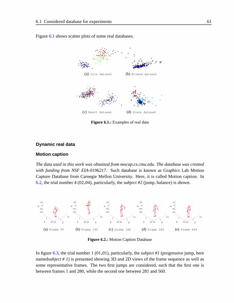
6.1 Considered database for experiments 61
Figure6.1shows scatter plots of some real databases.
(a) Iris dataset (b) Biomed dataset
(c) Heart dataset (d) Glass dataset
Figure 6.1.:Examples of real data
Dynamic real data
Motion caption
The data used in this work was obtained from mocap.cs.cmu.edu. The database was createdwith funding from NSF EIA-0196217. Such database is known as Graphics Lab MotionCapture Database from Carnegie Mellon University. Here, it is called Motion caption. In6.2, the trial number 4 (0204), particularly, thesubject #2(jump, balance) is shown.
0.51
1.5
0.5
1
−0.4
−0.2
0
0.2
XY
Z
(a) Frame 95
0.51
1.5
0.5
1
−0.4
−0.2
0
0.2
XY
Z
(b) Frame 140
0.51
1.5
0.5
1
−0.4
−0.2
0
0.2
XY
Z
(c) Frame 182
0.51
1.5
0.5
1
−0.4
−0.2
0
0.2
XY
Z
(d) Frame 280
0.51
1.5
0.5
1
−0.4
−0.2
0
0.2
XY
Z
(e) Frame 404
Figure 6.2.:Motion Caption Database
In figure6.3, the trial number 1 (0101), particularly, thesubject #1(progressive jump, herenamedsubject # 1) is presented showing 3D and 2D views of the frame sequence as well assome representative frames. The two first jumps are considered, such that the first one isbetween frames 1 and 280, while the second one between 281 and 560.
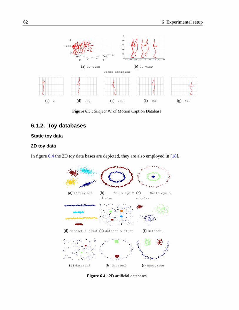
62 6 Experimental setup
0
0.5
10
0.51
0
0.5
1
X Y
Z(a) 3D view
−0.8 −0.6 −0.4 −0.2 0 0.2 0.4 0.6 0.80
0.2
0.4
0.6
0.8
1
Y
Z
(b) 2D view
Frame examples
XY
(c) 2 (d) 240 (e) 280 (f) 450 (g) 560
Figure 6.3.: Subject #1of Motion Caption Database
6.1.2. Toy databases
Static toy data
2D toy data
In figure6.4the 2D toy data bases are depicted, they are also employed in [18].
(a) 4Gaussians (b) Bulls eye 2
circles
(c) Bulls eye 3
circles
(d) dataset 4 clust (e) dataset 5 clust (f) dataset1
(g) dataset2 (h) dataset3 (i) HappyFace
Figure 6.4.:2D artificial databases
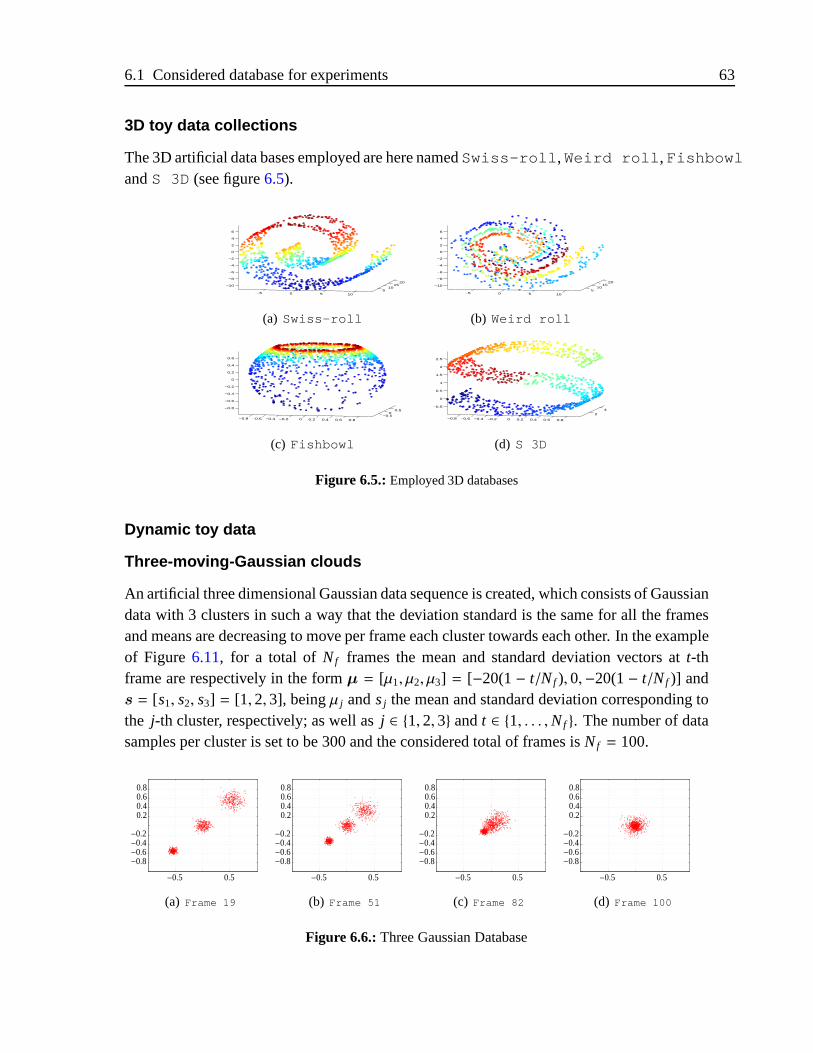
6.1 Considered database for experiments 63
3D toy data collections
The 3D artificial data bases employed are here namedSwiss-roll,Weird roll,FishbowlandS 3D (see figure6.5).
−5 0 5 105
1015
20−10
−8
−6
−4
−2
0
2
4
6
(a) Swiss-roll
−5 0 5 105
1015
20−10
−8
−6
−4
−2
0
2
4
6
(b) Weird roll
−0.8 −0.6 −0.4 −0.2 0 0.2 0.4 0.6 0.8−0.5
00.5
−0.8
−0.6
−0.4
−0.2
0
0.2
0.4
0.6
(c) Fishbowl
−0.8 −0.6 −0.4 −0.2 0 0.2 0.4 0.6 0.8
2
4−0.5
0
0.5
1
1.5
2
2.5
(d) S 3D
Figure 6.5.: Employed 3D databases
Dynamic toy data
Three-moving-Gaussian clouds
An artificial three dimensional Gaussian data sequence is created, which consists of Gaussiandata with 3 clusters in such a way that the deviation standard is the same for all the framesand means are decreasing to move per frame each cluster towards each other. In the exampleof Figure 6.11, for a total of Nf frames the mean and standard deviation vectors att-thframe are respectively in the formµ = [µ1, µ2, µ3] = [−20(1− t/Nf ), 0,−20(1− t/Nf )] ands = [s1, s2, s3] = [1, 2, 3], beingµ j andsj the mean and standard deviation corresponding tothe j-th cluster, respectively; as well asj ∈ 1, 2, 3 andt ∈ 1, . . . ,Nf . The number of datasamples per cluster is set to be 300 and the considered total of frames isNf = 100.
0.80.6
0.20.4
−0.8−0.6−0.4−0.2
0.5−0.5
(a) Frame 19
0.80.6
0.20.4
−0.8−0.6−0.4−0.2
0.5−0.5
(b) Frame 51
0.80.6
0.20.4
−0.8−0.6−0.4−0.2
0.5−0.5
(c) Frame 82
0.80.6
0.20.4
−0.8−0.6−0.4−0.2
0.5−0.5
(d) Frame 100
Figure 6.6.:Three Gaussian Database
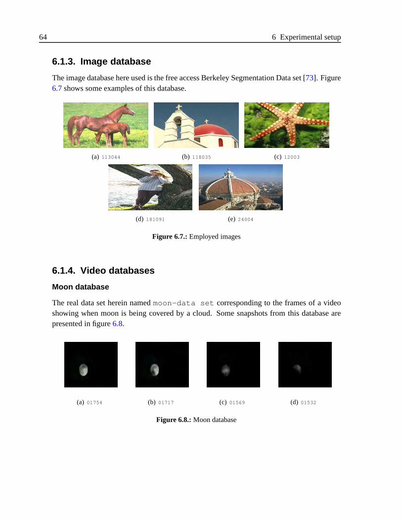
64 6 Experimental setup
6.1.3. Image database
The image database here used is the free access Berkeley Segmentation Data set [73]. Figure6.7shows some examples of this database.
(a) 113044 (b) 118035 (c) 12003
(d) 181091 (e) 24004
Figure 6.7.:Employed images
6.1.4. Video databases
Moon database
The real data set herein namedmoon-data set corresponding to the frames of a videoshowing when moon is being covered by a cloud. Some snapshots from this database arepresented in figure6.8.
(a) 01754 (b) 01717 (c) 01569 (d) 01532
Figure 6.8.: Moon database
6.2 Clustering Performance Measures 65
6.2. Clustering Performance Measures
This section describes the measures used to quantify the clustering performance regard-ing both supervised (section6.2.1) or unsupervised (section6.2.2) inferences depending onwhether the labels are known. Supervised measures are applied by comparing the groundtruth with the cluster indicators returned by the clustering algorithm. Also, two novel mea-sures are introduced in section
Throughout this section, consider aN-dimensional data set arranged in a data matrixX ∈R
N×d, which is to be clustered intoK clusters.
6.2.1. Supervised measures
Confusion matrix-derived measures
Nonetheless, this work takes advantage of the data set labels and therefore supervised mea-sures are accomplished. Thus, performance outcomes can be contrasted with another similarworks. In particular, each assembled cluster can be split into two clases: one holding themajority elements regarding to the class of interest (IC), and another having the minorityelements being of different classes (OC).
– True Positive (TP), the number of data pointsIC classified correctly.
– True negative (TN), the number of data pointsOC, classified correctly.
– False positive (FP), the number of data pointsOC classified asIC.
– False negative (FN), the number of data pointsIC classified asOC.
After computing the above described measures, the following values of sensitivity (S e),specificity (S p), and clustering performance (CP) are estimated as:
Se =TP
TP + FN
Sp =TN
TN + FP
CP =TN + TP
TN + FP + TP + FN
The sensibility and specificity quantify the proportion of elements fromIC and theOC thatare correctly classified, respectively. Both indexes measure the partition quality with respectto ideal case, when the quantity of clusters equates to the number of classes, but each clusterholding just one class.
66 6 Experimental setup
Nonetheless, there is no ideal partition, i.e., either, the number of clusters is lower than thenumber of classes, because the variables considered do not discriminate distinct classes or itshould be expected more clusters than classes. Besides, some clusters may contain majorityand minority elements from another classes. Therefore, the partition might be penalizedwhen holding a relatively large number of groups regarding number of classes, for instance,by means of a factor as
e−ηkr/ka (6.1)
wherekr is the number of groups resulting from the clustering,ka, is the admissibility valueof groups, andη, 0 < η ≤ 1, is an adjusting value. In this way, the measurem that can beSe, Sp or CP is weighted as follows:
m =
me−ηkr /ka, kr > ka
m, kr ≤ ka
The value ofηmust be greater than 0, and it can be less than 1 for a less rigorous penalization(0 < η ≤ 1).
Rand Index
Another supervised measure is the Rand index which takes advantage of labels given bydifferent partitions. Given a set ofN elementsX = x1, x2, . . . , xN, and two partitions ofX,V = v1, . . . , vR andU = u1, . . . , uC, such that
⋃Ri=1 vi = X =
⋃Cj=1 u j andvi
⋂vi′ = ∅ =
u j⋂
u j′ for 1 ≤ i , i′ ≤ R and 1≤ j , j′ ≤ C. SupposeV is the ground truth labels andU aclustering result. Leta be the number of pairs of objects that are placed in the same class inV and in te same cluster inU, b be the number of pairs of objects in the same class inV butnot in the same cluster inU, c be the number of pairs of objects in the same cluster inU butnot in the same class inV, andd be the number of pairs of objects in different classes anddifferent clusters in both partitions. Intuitively,a andd can be considered as the number ofagreements betweenU andV while b andc as disagreements. The Rand index [74], RI, is,
RI =a+ d
a+ b+ c+ d=
a+ d(N2
) (6.2)
The Rand index is in the range [0,1], with 0 indicating that the two partitions do not agreeon any pair of points and 1 when agree perfectly.A problem with the Rand index is that it does not guarantee that random label assignmentswill get a value close to zero, especially if the number of cluster is in the same order of mag-nitude as the number of samples, it means that the expected value of two random partitionsdoes not take a constant value. To counter this effect the adjusted Rand index is defined.
6.2 Clustering Performance Measures 67
Adjusted Rand Index
The adjusted Rand index, proposed by [75], is the corrected for chance version of the Randindex. It assumes the generalized hypergeometric distribution as the model of randomness,i.e., theV andU partitions are picked at random such that the number of objects in the classesand clusters are fixed. The overlap betweenV andU can be summarized in a contingencytable where each entryni j denotes the number of objects in common betweenVi andU j, ni·
andn· j denotes the number of objects in classvi and clusteru j respectively [76]. Table ofcontingency is illustrated in Table6.2.
Table 6.2.:contingency table for comparing two partitions
Class Cluster u1 u2 · · · uC Sumsv1 n11 n12 · · · n1C n1·
v2 n21 n22 · · · n2C n2·...
......
......
...
vR nR1 nR2 · · · nRC nR·
Sums n·1 n·2 · · · n·C n·· = N
The general form of an index with a constant expected value is,
ad justed index=index− expected index
max index− expected index
(6.3)
then, the adjusted Rand index (ARI), is
ARI =
∑i, j
(ni j
2
)−
[∑i
(ni·2
)∑j
(n· j2
)]/(
N2
)
12
[∑i
(ni·2
)+
∑j
(n· j2
)]−
[∑i
(ni·2
)∑j
(n· j2
)]/(
N2
) (6.4)
Normalized Mutual Information
Mutual information is an information theoretic based measure, which are built upon funda-mental concepts from information theory [77] and provides a sound indication of the sharedinformation between a pair of clusterings. LetI (U,V) denote the mutual information be-tweenU andV, andH(U) denote the entropy ofU, where,
H(U) = −C∑
i=1
n·iN
logn·iN, (6.5)
I (U,V) =C∑
i=1
R∑
j=1
ni j
Nlog
ni j/N
n·in j·/N2(6.6)

68 6 Experimental setup
SinceI (U,V) is a metric and has no upper bound, then for an easier interpretation and com-parisons, a normalized version ofI (U,V) that range from 0 to 1 is desirable. Several normal-izations are possible based on the observation thatI (U,V) ≤ min(H(U),H(V)), for this workis used a normalizing using the geometric mean, as follows [78],
NMI (U,V) =I (U,V)
√H(U)H(V)
(6.7)
This normalized variant is bounded in [0, 1], it is 1 when the two clusterings are identical, and0 when they sharing no information about each other. For a detailed description of mutualinformation normalizations see [79].
6.2.2. Unsupervised measures
Fisher Criterion , J
This measure quantifies how well each data point is grouped into clusters regarding theEuclidean distance-based compactness, which is estimated as follows:
J =
tr
(K∑
k=1
(xk −X
)⊤ (xk −X
))
tr
(K∑
k=1Sk
) , J ∈ R+ (6.8)
wherexk is the mean of thek-th cluster,X is the mean of the whole dataX ∈ RN×d, andSk
is the covariance matrix associated to clusterk. The number of groups,K, is chosen as theoriginal one regarding each tested database.
Silhouette, S
Silhouette measures how compact the formed clusters are through the within to betweencluster variance ratio [80], is estimated as:
S =1N
N∑
i=1
minbi
k
bi − ai
sup∀iai,minbi
, εs ∈ [−1, 1] (6.9)
whereai is the average distance from thei-th data point to the other points within thek-thcluster, vectorbi = [bi
1, . . . , biK] holds every valuebi
k, which is the average distance from thei-th point to points belonging to clusterk.
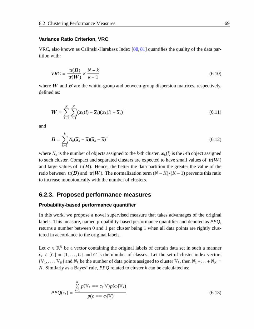
6.2 Clustering Performance Measures 69
Variance Ratio Criterion, VRC
VRC, also known as Calinski-Harabasz Index [80,81] quantifies the quality of the data par-tition with:
VRC=tr(B)tr(W )
× N − kk− 1
(6.10)
whereW andB are the whitin-group and between-group dispersion matrices, respectively,defined as:
W =
K∑
k=1
Ni∑
l=1
(xk(l) − xk)(xk(l) − xk)⊤ (6.11)
and
B =
k∑
k=1
Nk(xk − x)(xk − x)⊤ (6.12)
whereNk is the number of objects assigned to thek-th cluster,xk(l) is thel-th object assignedto such cluster. Compact and separated clusters are expected to have small values of tr(W )and large values of tr(B). Hence, the better the data partition the greater the value of theratio between tr(B) and tr(W ). The normalization term (N−K)/(K − 1) prevents this ratioto increase monotonically with the number of clusters.
6.2.3. Proposed performance measures
Probability-based performance quantifier
In this work, we propose a novel supervised measure that takes advantages of the originallabels. This measure, named probability-based performance quantifier and denoted asPPQ,returns a number between 0 and 1 per cluster being 1 when all data points are rightly clus-tered in accordance to the original labels.
Let c ∈ RN be a vector containing the original labels of certain data set in such a mannercℓ ∈ [C] = 1, . . . ,C andC is the number of classes. Let the set of cluster index vectorsV1, . . . ,VK andNk be the number of data points assigned to clusterVk, thenN1+ . . .+NK =
N. Similarly as a Bayes’ rule,PPQrelated to clusterk can be calculated as:
PPQ(cℓ) =
K∑k=1
p(Vk == cℓ|V)p(cℓ |Vk)
p(c == cℓ|V)(6.13)

70 6 Experimental setup
where p(Vk == cℓ|V) is the probability that data points labeled withcℓ are grouped intoclusterk:
p(Vk == cℓ|V) =ne(Vk == cℓ)
N, (6.14)
p(cℓ |Vk) is the relative probability that data points labeled withcℓ are grouped ask regardingits own cluster
p(cℓ|Vk) =ne(Vk == cℓ)
Nℓ
, (6.15)
p(cℓ |V) is the total probability that a data point can be grouped ask-labeled
p(cℓ|V) =ne(c == cℓ)
N(6.16)
andne(·) denotes the number of nodes satisfying its argument condition. Termp(cℓ|Vk) worksas a penalty factor avoiding that measure value becomes one in all cases, since it ceases be-ing 1 in case of wrongly assignments, i.e., when there are label-mixed clusters.
To understand better how to apply thePPQ, let us consider the example given in Figure6.9.
11
1
1
1
2
23
3
3
V1 V2 V3
Figure 6.9.:Example for explanation ofPPQmeasure considering three clusters and three classes
According to the example, we have:
PPQ(1) =P(V1 == 1|V)P(V1|V1) + P(V1 == 2|V)P(V1|V2) + P(V1 == 3|V)P(V1|V3)
P(V1|V)
=(0.3)(1)+ (0.2)(1)+ (0)(0)
0.5= 1
PPQ(2) =P(V2 == 1|V)P(V2|V1) + P(V2 == 2|V)P(V2|V2) + P(V2 == 3|V)P(V2|V3)
P(V2|V)
PPQ(2) =(0)(0)+ (0)(0)+ (0.4)(0.2)
0.2= 0.4
PPQ(3) =P(V3 == 1|V)P(V3|V1) + P(V3 == 2|V)P(V3|V2) + P(V3 == 3|V)P(V3|V3)
P(V3|V)
PPQ(3) =(0)(0)+ (0)(0)+ (0.6)(0.3)
0.3= 0.6
6.2 Clustering Performance Measures 71
Notice that, despite spending two clusters, class labeled 1 achieves aPPQequals to 1. Thisis because there is no mixed labels inside the cluster assignment, in contrast to the the tworemaining clusters.
Cluster coherence
As another cluster validity measure to be considered, clustering quality is assessed that isbased on spectral graph partitioning [8], when a good clustering desires both tight connec-tions within partitions and loose connections between partitions. Thus, the cluster coherenceis calcules as follows:
ǫM =1k
k∑
l=1
MTl ΩMl
MTl DMl
(6.17)
whereM is the matrix formed by the membership values of all elements to each cluster:mi j = m(q j/xi), Ml denotes a membership submatrix associated to the clusterl, Ω is theassumed similarity matrix andD is the degree of matrixΩ. Due to normalization withrespect to the similarity matrix, the maximum value ofεM is 1, therefore, it indicates a goodclustering if its value is near 1. Furthermore, because of the nature of the function, a largeset of groups is penalized.
72 6 Experimental setup
6.3. Experiment description
This section describes the experiments carried out to assess the performance of the improvedKSC (PKSC), as well as Dynamic clustering approach based on MKL, involving tracking(KSCT) and dynamic KSC (DKSC).
6.3.1. Experiments for assessing the projected KSCperformance
The proposed method, termed Projected Kernel Spectral Clustering (PKSC) is comparedwith the baseline KSC, multi-cluster spectral clustering [8], as well as the standard K-means [82]. Clustering performance is assessed on both training and test sets extractedfrom artificial and real databases described in section6.1. The employed measures used toquantify the clustering performance are the Fisher criterion, silhouette index, and the clustercoherence as explained in appendix6.2.
As a result, it is shown that PKSC improves the performance of the baseline kernel spectralclustering, but also outperforms the another compared clustering methods.
6.3.2. Experiments for KSC-based tracking
Some experiments are carried out considering two databases: Motion Caption and an artifi-cial three-moving Gaussian, which are in detail described in appendix6.1. Proposed trackingis assessed regarding the clustering performance by KSC (chapter4), kernel K-means (Ap-pendix A) and Min-Cuts [70].
To quantify the clustering performance, normalized mutual information and adjusted randomindex metrics are used, as described in section6.2. In general, obtained results show clearlythat there exists a direct relationship between the proposed tracking vector and the analyzeddynamic data.
Databases
Motion caption: For experiments, we use the trial number 4 (0204) of motion captiondatabase, particularly, thesubject #2(jump, balance). Each frame is in size 38× 3 rep-resenting the coordinatesX, Y and Z of the subject’s body points, therefore eachx
(t)i is
114-dimensional. Since 484 frames are considered, data matrix at time instancet is X (t) isin size 484×114. This database is described in section6.1.1. Some sample frames are shownin 6.10.
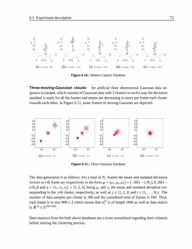
6.3 Experiment description 73
0.51
1.5
0.5
1
−0.4
−0.2
0
0.2
XY
Z
(a) Frame 95
0.51
1.5
0.5
1
−0.4
−0.2
0
0.2
XYZ
(b) Frame 140
0.51
1.5
0.5
1
−0.4
−0.2
0
0.2
XY
Z
(c) Frame 182
0.51
1.5
0.5
1
−0.4
−0.2
0
0.2
XY
Z
(d) Frame 280
0.51
1.5
0.5
1
−0.4
−0.2
0
0.2
XY
Z
(e) Frame 404
Figure 6.10.:Motion Caption Database
Three-moving-Gaussian clouds: An artificial three dimensional Gaussian data se-quence is created, which consists of Gaussian data with 3 clusters in such a way the deviationstandard is static for all the frames and means are decreasing to move per frame each clustertowards each other. In Figure6.11, some frames of moving Gaussian are depicted.
0.80.6
0.20.4
−0.8−0.6−0.4−0.2
0.5−0.5
(a) Frame 19
0.80.6
0.20.4
−0.8−0.6−0.4−0.2
0.5−0.5
(b) Frame 51
0.80.6
0.20.4
−0.8−0.6−0.4−0.2
0.5−0.5
(c) Frame 82
0.80.6
0.20.4
−0.8−0.6−0.4−0.2
0.5−0.5
(d) Frame 100
Figure 6.11.:Three Gaussian Database
The data generation is as follows: For a total ofNf frames the mean and standard deviationvectors att-th frame are respectively in the formµ = [µ1, µ2, µ3] = [−20(1− t/Nf ), 0, 20(1−t/Nf )] ands = [s1, s2, s3] = [1, 2, 3], beingµ j andsj the mean and standard deviation cor-responding to thej-th cluster, respectively; as well asj ∈ 1, 2, 3 andt ∈ 1, . . . ,Nf . Thenumber of data samples per cluster is 300 and the considered total of frames is 100. Thus,each frame is in size 900× 2 which means thatx(t)
i is of length 1800 as well as data matrixisX (t) ∈ R100×1800.
Data matrices from the both above databases arez-score normalized regarding their columnsbefore starting the clustering process.
74 6 Experimental setup
Clustering and Kernel Parameters
Al l the experiments are performed under specific initial parameters, namely, the number ofclustersK and kernel function. For Motion Caption database (subject #2), parameterK is setto be 5. In case of moving Gaussian, we empirically determine thatK = 4. The consideredkernel for both cases is the local-scaled Gaussian kernel as explained in section4.2 (section4.2.2). Free kernel scaling parameterm is empirically set by varying it within an interval andthen it is chosen as that one achieving greatest Fisher’s criterion value. In the case of MotionCaption, we obtainm= 35; whilem= 10 for the moving Gaussian.
For comparison purposes, kernel K-means (KKM) and Min-Cuts are also considered [70].The clustering performance is quantified by two metrics: normalized mutual information(NMI) and adjusted random index (ARI) calculated as explained in section6.2. Both metricsreturn values ranged into the interval [0, 1], being closer than 1 when better is the clusteringperformance.
6.3.3. Experiments for Dynamic KSC
Experiments are carried out using two databases. On one hand, a subject from Graphics LabMotion Capture Database from Carnegie Mellon University, here called Motion Caption. Onthe other hand, an artificial three-moving Gaussian clouds in which the mean of each cloudis changed along the frames.
For comparison purposes, some conventional spectral clustering techniques are also con-sidered, namely, kernel k-means (KKM) and min-cuts (MC) [70]. Also, standard K-means(KM) is considered. The normalized mutual information (NMI) and adjusted random index(ARI) metrics are used to quantify the clustering performance. The introduced PPQ measureis considered as well, which is explained in section6.2.
Databases
Motion caption: In this work, we use the trial number 1 (0101), particularly, thesubject#1 (progressive jump). The two first jumps are considered, such that the first one is betweenframes 1 and 280, while the second one between 281 and 560. Each frameX (t) per jumpis in size 280× 114 whose rows contain the vectorization of coordinatesX, Y andZ of thesubject’s body points, therefore each ˆxi is the dimension of 31920. Note that we considertwo jumps which meansNf m = 2. Then, frame matrixX is in size 2×31920. In Figure6.12,the subject # 1sequence is presented showing 3D and 2D views of the frame sequence aswell as some representative frames.
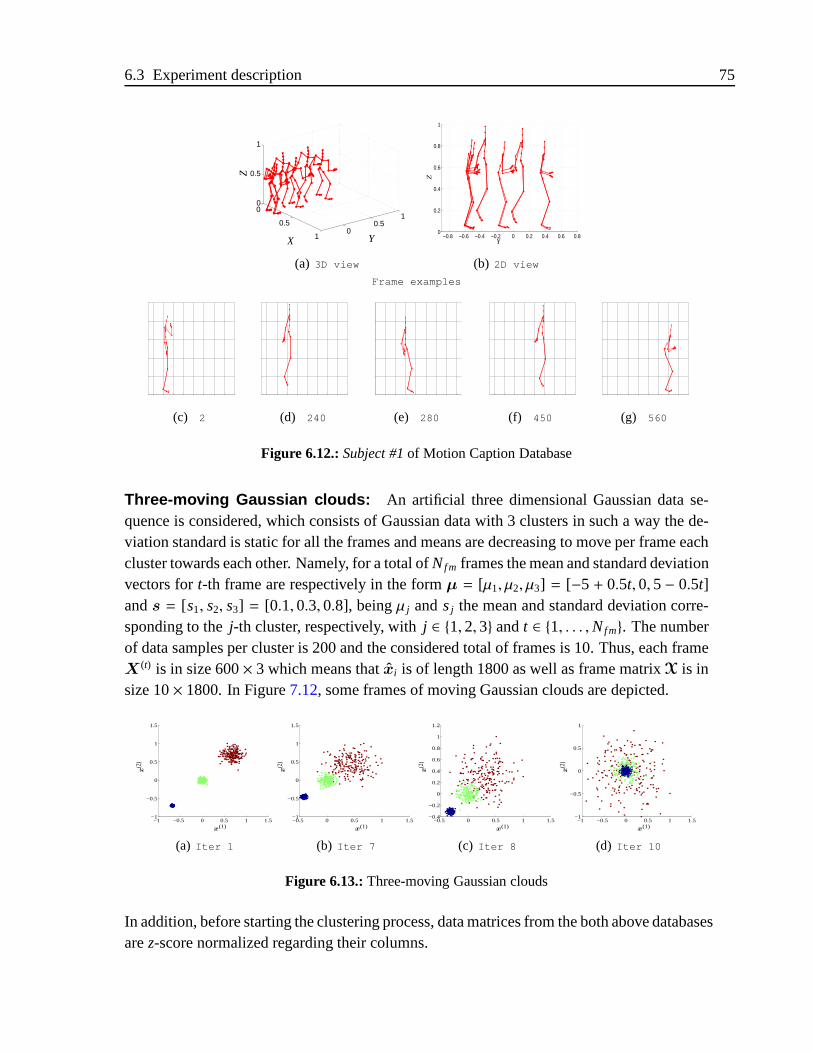
6.3 Experiment description 75
0
0.5
10
0.51
0
0.5
1
X YZ
(a) 3D view
−0.8 −0.6 −0.4 −0.2 0 0.2 0.4 0.6 0.80
0.2
0.4
0.6
0.8
1
Y
Z
(b) 2D view
Frame examples
(c) 2 (d) 240 (e) 280 (f) 450 (g) 560
Figure 6.12.:Subject #1of Motion Caption Database
Three-moving Gaussian clouds: An artificial three dimensional Gaussian data se-quence is considered, which consists of Gaussian data with 3 clusters in such a way the de-viation standard is static for all the frames and means are decreasing to move per frame eachcluster towards each other. Namely, for a total ofNf m frames the mean and standard deviationvectors fort-th frame are respectively in the formµ = [µ1, µ2, µ3] = [−5 + 0.5t, 0, 5− 0.5t]ands = [s1, s2, s3] = [0.1, 0.3, 0.8], beingµ j andsj the mean and standard deviation corre-sponding to thej-th cluster, respectively, withj ∈ 1, 2, 3 andt ∈ 1, . . . ,Nf m. The numberof data samples per cluster is 200 and the considered total of frames is 10. Thus, each frameX (t) is in size 600× 3 which means that ˆxi is of length 1800 as well as frame matrixX is insize 10× 1800. In Figure7.12, some frames of moving Gaussian clouds are depicted.
−1 −0.5 0 0.5 1 1.5−1
−0.5
0
0.5
1
1.5
x(1)
x(2
)
(a) Iter 1
−0.5 0 0.5 1 1.5−1
−0.5
0
0.5
1
1.5
x(1)
x(2
)
(b) Iter 7
−0.5 0 0.5 1 1.5−0.4
−0.2
0
0.2
0.4
0.6
0.8
1
1.2
x(1)
x(2
)
(c) Iter 8
−1 −0.5 0 0.5 1 1.5−1
−0.5
0
0.5
1
x(1)
x(2
)
(d) Iter 10
Figure 6.13.:Three-moving Gaussian clouds
In addition, before starting the clustering process, data matrices from the both above databasesarez-score normalized regarding their columns.
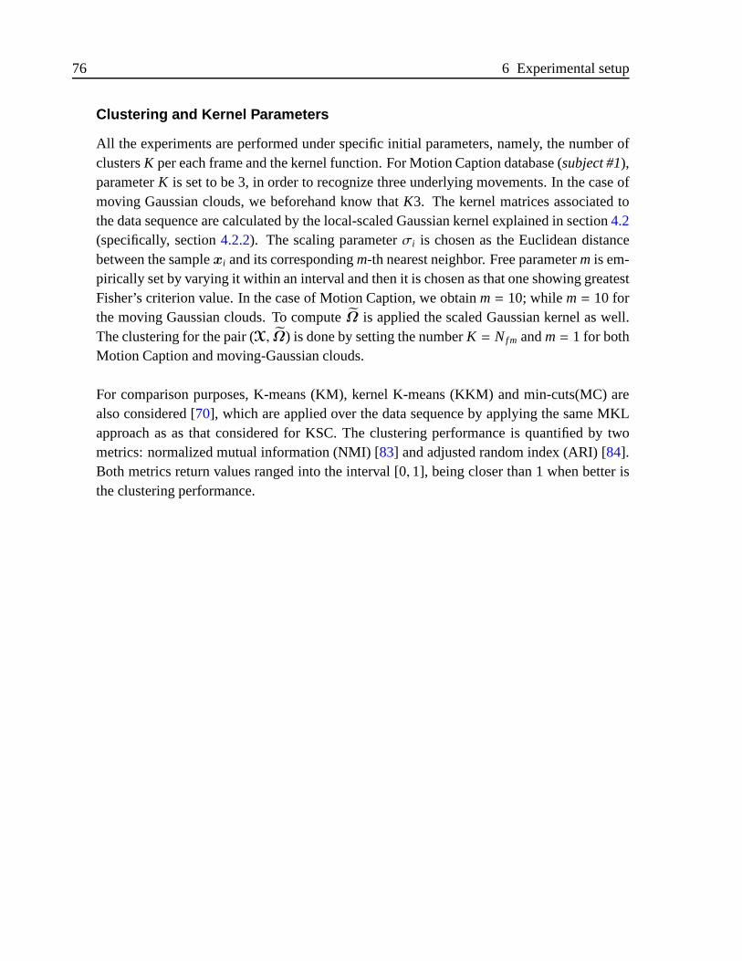
76 6 Experimental setup
Clustering and Kernel Parameters
Al l the experiments are performed under specific initial parameters, namely, the number ofclustersK per each frame and the kernel function. For Motion Caption database (subject #1),parameterK is set to be 3, in order to recognize three underlying movements. In the case ofmoving Gaussian clouds, we beforehand know thatK3. The kernel matrices associated tothe data sequence are calculated by the local-scaled Gaussian kernel explained in section4.2(specifically, section4.2.2). The scaling parameterσi is chosen as the Euclidean distancebetween the samplexi and its correspondingm-th nearest neighbor. Free parameterm is em-pirically set by varying it within an interval and then it is chosen as that one showing greatestFisher’s criterion value. In the case of Motion Caption, we obtainm= 10; whilem= 10 forthe moving Gaussian clouds. To computeΩ is applied the scaled Gaussian kernel as well.The clustering for the pair (X, Ω) is done by setting the numberK = Nf m andm= 1 for bothMotion Caption and moving-Gaussian clouds.
For comparison purposes, K-means (KM), kernel K-means (KKM) and min-cuts(MC) arealso considered [70], which are applied over the data sequence by applying the sameMKLapproach as as that considered for KSC. The clustering performance is quantified by twometrics: normalized mutual information (NMI) [83] and adjusted random index (ARI) [84].Both metrics return values ranged into the interval [0,1], being closer than 1 when better isthe clustering performance.
7. Results and discussion
7.1. Results for experiments of projected KSC (PKSC)
7.1.1. Clustering Results of Three-Gaussian Data Sets
Quality of assessed clustering is provided for all considered methods by using the scat-ter plots that are shown in Figure7.1, which are obtained assuming a mean vectorµ =
[µ1, µ2, µ3] and a standard deviation vectors = [s1, s2, s3], beingµi andsi the mean and stan-dard deviation corresponding toi−th cluster, respectively. Namely, clustering is performedfor two a priori fixed values of separability: lower separability (i.e.,µ = [−0.3, 0, 0.3], ands = [0.1, 0.2, 0.3]), and a high separability (i.e.,µ = [−1.8, 0, 1.8] ands = [0.1, 0.2, 0.3]).
As expected, all considered methods (including PKSC) properly determine each one of theclusters when they are linearly separable (see left column of Figure7.1), is when taking thehigh level of separability. If assuming the low level of separability, when clusters becomecloser each other (i.e., by reducing the means), theK-means technique yields three closelybalanced groups, as seen in right column of Figure7.1.
This fact can be explained sinceK-means is a center-based clustering, which seeks the mini-mization of the within-cluster variance and centers are updated per iteration within a heuristicsearch. In contrast, both KSC and MCSC are not longer able to form the three desired mul-tidimensional clusters. Instead, they accomplish a big cluster along with other two smallclusters that rather should be assumed as outliers. This fact may be explained since bothKSC and MCSC evaluate the data local structure, i.e., they consider the local dissimilarityamong points estimated by an RBF kernel for a given scale parameterσ. In other words, bothmethods form clusters in accordance the chosen parameterσ. Furthermore, the selectedσis adequate for PKSC, but it is not enough neither for MCSC nor for KSC. For compact andclose clusters, therefore, MCSC and KSC require a more thorough search for selecting thebandwidth parameter than the proposed method. As regards the proposed PKSC method,because of introduced projection one can see that it yields a suitable representation spaceallowing to estimate more accurately the number of groups, when clusters become closereach other. Figure7.2 shows the estimated box plots for all considered clustering methodsfor both assumed separability levels.
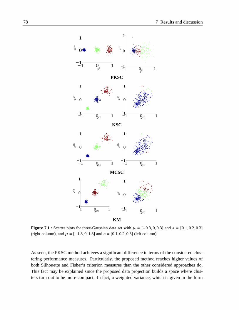
78 7 Results and discussion
−1 0 1−1
0
1
y(1)
y(2
)
−1 0 1−1
0
1
y(1)
y(2
)
PKSC
−1 0 1−1
0
1
x(1)
x(2
)
−1 0 1−1
0
1
x(1)x
(2)
KSC
−1 0 1−1
0
1
x(1)
x(2
)
−1 0 1−1
0
1
x(1)
x(2
)
MCSC
−1 0 1−1
0
1
x(1)
x(2
)
−1 0 1−1
0
1
x(1)
x(2
)
KM
Figure 7.1.: Scatter plots for three-Gaussian data set withµ = [−0.3, 0, 0.3] ands = [0.1, 0.2, 0.3](right column), andµ = [−1.8, 0, 1.8] ands = [0.1, 0.2, 0.3] (left column)
As seen, the PKSC method achieves a significant difference in terms of the considered clus-tering performance measures. Particularly, the proposed method reaches higher values ofboth Silhouette and Fisher’s criterion measures than the other considered approaches do.This fact may be explained since the proposed data projection builds a space where clus-ters turn out to be more compact. In fact, a weighted variance, which is given in the form
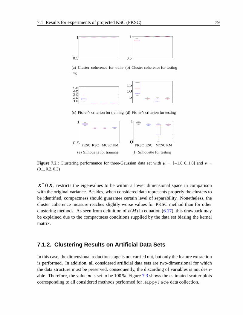
7.1 Results for experiments of projected KSC (PKSC) 79
0.5
1
(a) Cluster coherence for train-ing
0.5
1
(b) Cluster coherence for testing
1020304050
(c) Fisher’s criterion for training
5
10
15
(d) Fisher’s criterion for testing
0.5
1
PKSC KSC MCSC KM
(e) Silhouette for training
1
0PKSC KSC MCSC KM
(f) Silhouette for testing
Figure 7.2.: Clustering performance for three-Gaussian data set withµ = [−1.8, 0, 1.8] ands =
(0.1, 0.2, 0.3)
X⊤ΩX , restricts the eigenvalues to be within a lower dimensional space in comparison
with the original variance. Besides, when considered data represents properly the clusters tobe identified, compactness should guarantee certain level of separability. Nonetheless, thecluster coherence measure reaches slightly worse values for PKSC method than for otherclustering methods. As seen from definition ofε(M) in equation (6.17), this drawback maybeexplained due to the compactness conditions supplied by the data set biasing the kernelmatrix.
7.1.2. Clustering Results on Artificial Data Sets
In this case, the dimensional reduction stage is not carried out, but only the feature extractionis performed. In addition, all considered artificial data sets are two-dimensional for whichthe data structure must be preserved, consequently, the discarding of variables is not desir-able. Therefore, the valuem is set to be 100 %.Figure7.3shows the estimated scatter plotscorresponding to all considered methods performed forHappyFace data collection.
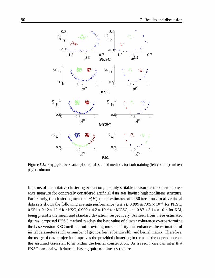
80 7 Results and discussion
x(2
)x(1)
0.3
0
-0.3-1.3 -1 -0.7
x(1)
0.3
0
-0.3-1.3 -1 -0.7
x(2
)
PKSC
0 0.5 10.5
1
(2)
(1)
x
x
0 0.5 10.5
1
(2)
(1)
x
xKSC
0 0.5 10.5
1
(2)
(1)
x
x
0 0.5 10.5
1
(2)
(1)
x
xMCSC
0 0.5 10.5
1
(2)
(1)
x
x
0 0.5 10.5
1
(2)
(1)
x
xKM
Figure 7.3.:HappyFace scatter plots for all studied methods for both training (left column) and test(right column)
In terms of quantitative clustering evaluation, the only suitable measure is the cluster coher-ence measure for concretely considered artificial data sets having high nonlinear structure.Particularly, the clustering measure,ε(M), that is estimated after 50 iterations for all artificialdata sets shows the following average performance (µ ± s): 0.999± 7.05× 10⁻⁴ for PKSC,0.951± 9.12× 10⁻³ for KSC, 0.990± 4.2× 10⁻³ for MCSC, and 0.87± 3.14× 10⁻³ for KM,beingµ ands the mean and standard deviation, respectively. As seen from these estimatedfigures, proposed PKSC method reaches the best value of cluster coherence overperformingthe base version KSC method, but providing more stability that enhances the estimation ofinitial parameters such as number of groups, kernel bandwidth, and kernel matrix. Therefore,the usage of data projection improves the provided clustering in terms of the dependence onthe assumed Gaussian form within the kernel construction. As a result, one can infer thatPKSC can deal with datasets having quite nonlinear structure.
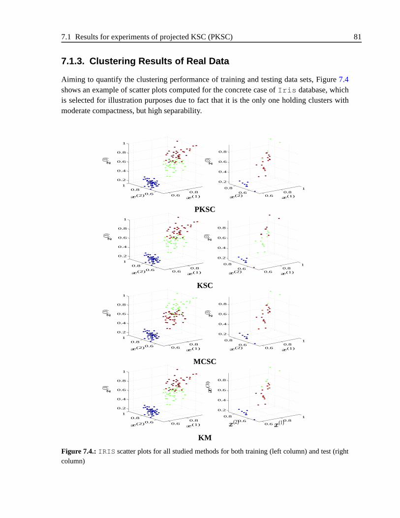
7.1 Results for experiments of projected KSC (PKSC) 81
7.1.3. Clustering Results of Real Data
Aiming to quantify the clustering performance of training and testing data sets, Figure7.4shows an example of scatter plots computed for the concrete case ofIris database, whichis selected for illustration purposes due to fact that it is the only one holding clusters withmoderate compactness, but high separability.
0.60.80.6
0.81
0.2
0.4
0.6
0.8
1
x(1)x(2)
x(3)
0.60.8
10.6
0.8
0.2
0.4
0.6
0.8
x(1)x(2)
x(3)PKSC
0.60.80.6
0.81
0.2
0.4
0.6
0.8
1
x(1)x(2)
x(3)
0.60.8
10.6
0.8
0.2
0.4
0.6
0.8
x(1)x(2)
x(3)
KSC
0.60.80.6
0.81
0.2
0.4
0.6
0.8
1
x(1)x(2)
x(3)
0.60.8
10.6
0.8
0.2
0.4
0.6
0.8
x(1)x(2)
x(3)
MCSC
0.60.80.6
0.81
0.2
0.4
0.6
0.8
1
x(1)x(2)
x(3)
0.60.8
10.6
0.8
0.2
0.4
0.6
0.8
x(1)x(2)
x(3
)
KM
Figure 7.4.:IRIS scatter plots for all studied methods for both training (left column) and test (rightcolumn)

82 7 Results and discussion
As seen, the KM method infers correctly all three corresponding compact clusters. Moreover,because of relaxed compactness and separability properties ofIris database, the Euclideandistance along with the centroid-based searching lead to a suitable clustering providing sim-ilar results in both training and test procedures. In case of MCSC method, although theclustering performs properly in training procedure due to the separability property of data,MCSC method fails during test procedure due to the presence of two overlapped clusters.As a result, clustering forms one big cluster and another small one instead of an expectedcouple of balanced clusters. This drawback can be explained due to the low accuracy of thedissimilarity matrix, which is estimated by using an RBF when clustering parameters are notproperly enough selected.
In case of KSC method, even though the clustering performs well in the training set, KSCinfers a lower number of groups (K = 2). This flaw is caused by the suboptimal estimationof bandwidth parameterσ that is carried out by encoding where the number of groups isestimated, as remarked in [21].
Lastly, the proposed PKSC method performs correctly clustering in both training and testprocedures. The introduced data projection improves the assignment to each data point,since the data is mapped by using an ortonormal basis of the eigenvectors of the weightedcovariance matrix related to local dissimilarities.
Besides of a better performed clustering among compared techniques, the PKSC methoddoes not require for an exhaustive searching during the tuning of parameterσ, and therefore,it reduces the computational burden. For quantitative evaluation of compared clusteringmethods, the estimated mean value of considered measures are shown in Table7.1, whichare computed after 50 iterations. It must be quoted that for the concrete case of PKSC, di-mensionp is fixed to bem= 99% to preserve most of the explained variance when carryingout the dimensionality reduction process.
The table is organized in such a manner that shown data sets are sorted increasingly withrespect to complexity structure from top to bottom. To quantify such complexity, Fisher’scriterion is chosen because it measures the ratio of within- and between- variance. As ref-erence method to arrange the Table, we select KM because of its simplicity and under theassumption that this method is appropriate to cluster data guaranteeing a relatively high com-pactness degree. This assumption is often satisfied by real data when data points adequatelyrepresent the clusters to be formed
An estimation of the clustering gain process can be given as the absolute difference betweenthe clustering performance achieved by each method and the one reached by the baselineKM method.
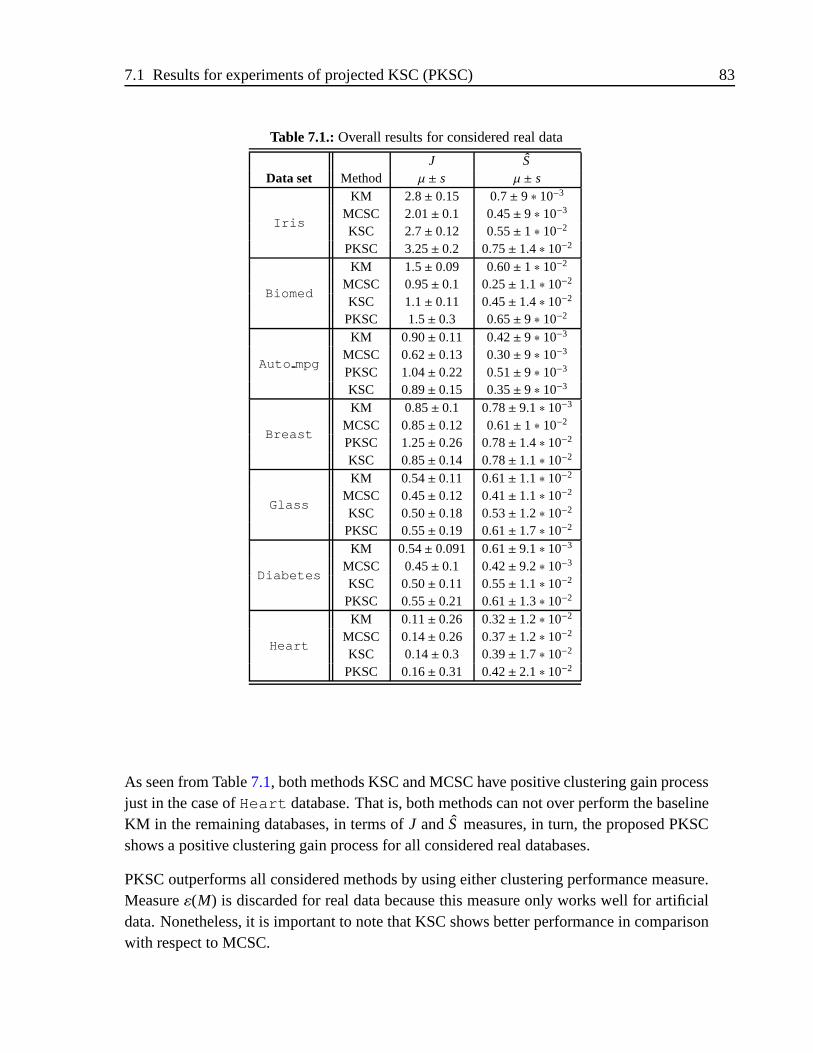
7.1 Results for experiments of projected KSC (PKSC) 83
Table 7.1.:Overall results for considered real data
J SData set Method µ ± s µ ± s
Iris
KM 2.8± 0.15 0.7± 9 ∗ 10−3
MCSC 2.01± 0.1 0.45± 9 ∗ 10−3
KSC 2.7± 0.12 0.55± 1 ∗ 10−2
PKSC 3.25± 0.2 0.75± 1.4 ∗ 10−2
Biomed
KM 1.5± 0.09 0.60± 1 ∗ 10−2
MCSC 0.95± 0.1 0.25± 1.1 ∗ 10−2
KSC 1.1± 0.11 0.45± 1.4 ∗ 10−2
PKSC 1.5± 0.3 0.65± 9 ∗ 10−2
Auto mpg
KM 0.90± 0.11 0.42± 9 ∗ 10−3
MCSC 0.62± 0.13 0.30± 9 ∗ 10−3
PKSC 1.04± 0.22 0.51± 9 ∗ 10−3
KSC 0.89± 0.15 0.35± 9 ∗ 10−3
Breast
KM 0.85± 0.1 0.78± 9.1 ∗ 10−3
MCSC 0.85± 0.12 0.61± 1 ∗ 10−2
PKSC 1.25± 0.26 0.78± 1.4 ∗ 10−2
KSC 0.85± 0.14 0.78± 1.1 ∗ 10−2
Glass
KM 0.54± 0.11 0.61± 1.1 ∗ 10−2
MCSC 0.45± 0.12 0.41± 1.1 ∗ 10−2
KSC 0.50± 0.18 0.53± 1.2 ∗ 10−2
PKSC 0.55± 0.19 0.61± 1.7 ∗ 10−2
Diabetes
KM 0.54± 0.091 0.61± 9.1 ∗ 10−3
MCSC 0.45± 0.1 0.42± 9.2 ∗ 10−3
KSC 0.50± 0.11 0.55± 1.1 ∗ 10−2
PKSC 0.55± 0.21 0.61± 1.3 ∗ 10−2
Heart
KM 0.11± 0.26 0.32± 1.2 ∗ 10−2
MCSC 0.14± 0.26 0.37± 1.2 ∗ 10−2
KSC 0.14± 0.3 0.39± 1.7 ∗ 10−2
PKSC 0.16± 0.31 0.42± 2.1 ∗ 10−2
As seen from Table7.1, both methods KSC and MCSC have positive clustering gain processjust in the case ofHeart database. That is, both methods can not over perform the baselineKM in the remaining databases, in terms ofJ andS measures, in turn, the proposed PKSCshows a positive clustering gain process for all considered real databases.
PKSC outperforms all considered methods by using either clustering performance measure.Measureε(M) is discarded for real data because this measure only works well for artificialdata. Nonetheless, it is important to note that KSC shows better performance in comparisonwith respect to MCSC.
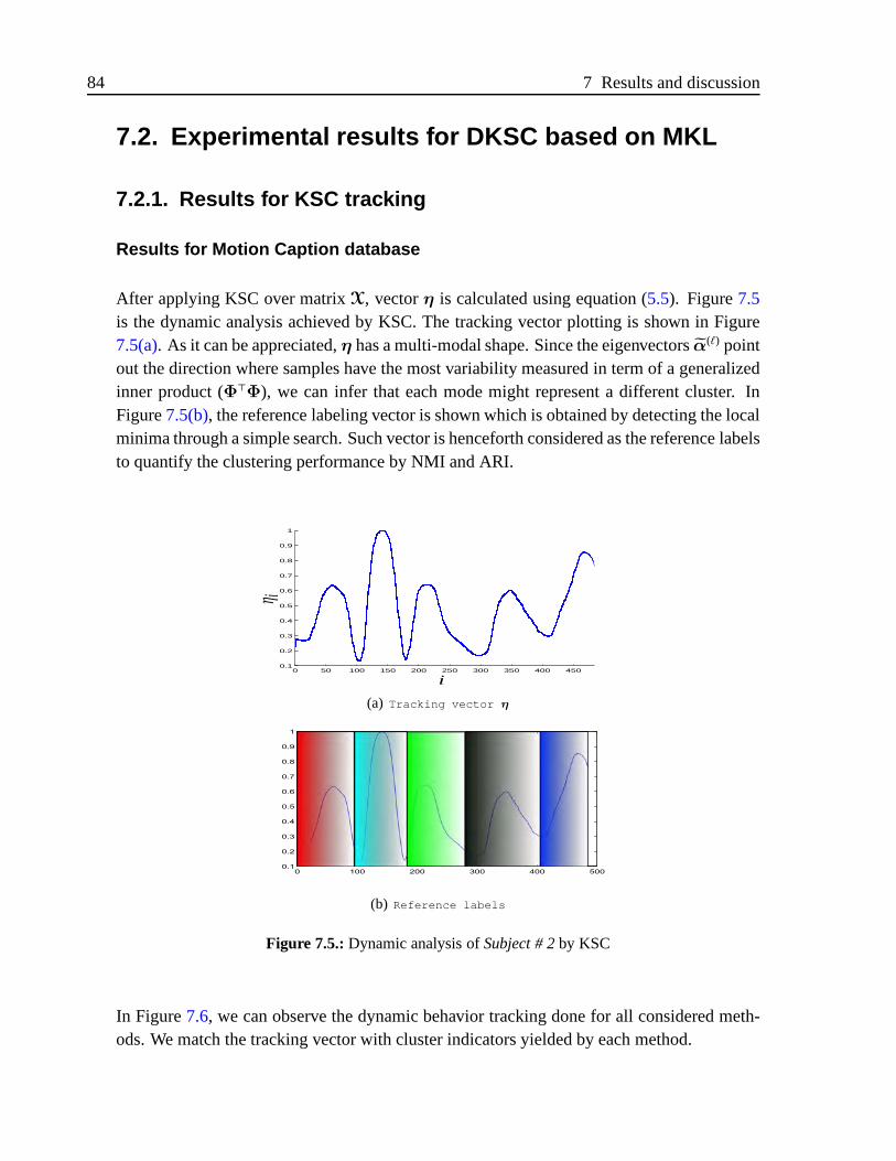
84 7 Results and discussion
7.2. Experimental results for DKSC based on MKL
7.2.1. Results for KSC tracking
Results for Motion Caption database
After applying KSC over matrixX, vectorη is calculated using equation (5.5). Figure7.5is the dynamic analysis achieved by KSC. The tracking vector plotting is shown in Figure7.5(a). As it can be appreciated,η has a multi-modal shape. Since the eigenvectorsα(ℓ) pointout the direction where samples have the most variability measured in term of a generalizedinner product (Φ⊤Φ), we can infer that each mode might represent a different cluster. InFigure7.5(b), the reference labeling vector is shown which is obtained by detecting the localminima through a simple search. Such vector is henceforth considered as the reference labelsto quantify the clustering performance by NMI and ARI.
0 50 100 150 200 250 300 350 400 4500.1
0.2
0.3
0.4
0.5
0.6
0.7
0.8
0.9
1
η i
i
(a) Tracking vector η
0 100 200 300 400 5000.1
0.2
0.3
0.4
0.5
0.6
0.7
0.8
0.9
1
(b) Reference labels
Figure 7.5.:Dynamic analysis ofSubject # 2by KSC
In Figure7.6, we can observe the dynamic behavior tracking done for all considered meth-ods. We match the tracking vector with cluster indicators yielded by each method.

7.2 Experimental results for DKSC based on MKL 85
0.2
0.4
0.6
0.8
1
100 200 300 400 500
(a) Reference Labels
0.2
0.4
0.6
0.8
1
100 200 300 400 500
(b) KSC
0.2
0.4
0.6
0.8
1
100 200 300 400 500
(c) KKM
0.2
0.4
0.6
0.8
1
100 200 300 400 500
(d) Min-Cuts
Figure 7.6.: Clustering results forSubject # 2
It is easy to appreciate that KSC performs a better clustering in comparison to the other meth-ods. This fact can be attributed to the coherence and evident linkage between the trackingvector and KSC. Also, note that the samples are organized in sequence, then we expect resul-tant clusters contain no isolated or disconnected (out of sequence) samples. In other words,clustering indicators reach low values when samples or frames are intermittently clusteredalong time. Then, KKM and Min-Cuts generate partially wrong grouping. Nevertheless, it isworth mentioning that this experimental framework was done with a specific type of kernelas well as a determined parameter tuning, i.e., maximal Fisher’s criterion in this case. Thus,it is possible that such a tuning process may not be appropriate for those methods. Albeit, itmust be taken into account that Fisher’s criterion is applied regardless the method, that is tosay that tuning process is done considering no the clustering method but the nature of databy means of the within- and between-variance ratio (Fisher’s criterion). The trial 4 (0204)is a vertical jump as shown.
Then, by comparing Figure6.10with Figure7.5, we can appreciate that the identified localminima determine five clusters representing five dynamic instances along time, associatedto subject #2. We name those clusters as follows:starting jump(between frames 1 and 95),jumping on the air(between frames 96 and 182),arrival to the ground(between frames 183and 280),back step(between 281 and 404) andquiet – Standing(between frames 405 and484).
The direct relationship between tracking vectorη and the partition of natural movementsfrom Subject #2can be plainly appreciated in Figure7.7, where the top row shows onerepresentative frame per cluster (in different color) while bottom row depicts theη curveuntil the last frame of the corresponding cluster.As expected, each mode – frames between inflections forming a concave curve – fromη plot-ting corresponds to a natural cluster, which may even be determined by simple inspection.The tracking effect can also be verified in Table7.2. In terms of the considered measures,wecan observe that KSC outperforms both KKM and Min-Cuts, which means that the clus-tering method might be coherent with the tracking procedure. In this connection, KSC is the
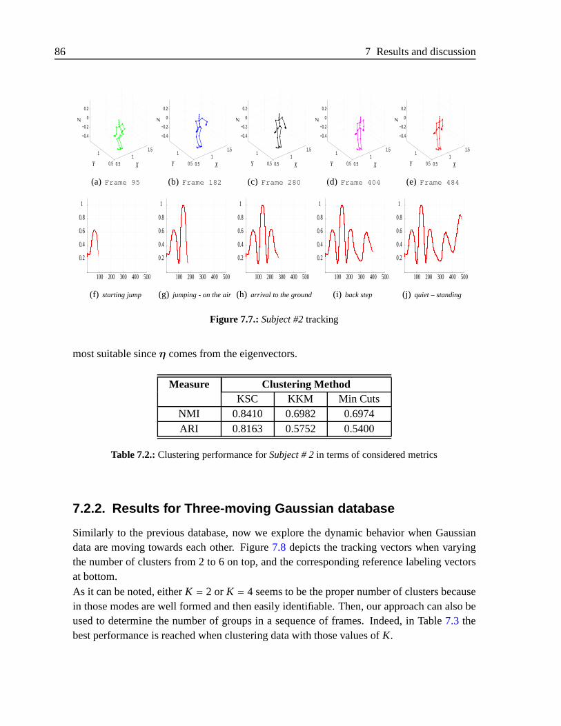
86 7 Results and discussion
0.51
1.5
0.5
1
−0.4
−0.2
0
0.2
XY
Z
(a) Frame 95
0.51
1.5
0.5
1
−0.4
−0.2
0
0.2
XYZ
(b) Frame 182
0.51
1.5
0.5
1
−0.4
−0.2
0
0.2
XY
Z
(c) Frame 280
0.51
1.5
0.5
1
−0.4
−0.2
0
0.2
XY
Z
(d) Frame 404
0.51
1.5
0.5
1
−0.4
−0.2
0
0.2
XY
Z
(e) Frame 484
0.2
0.4
0.6
0.8
1
100 200 300 400 500
(f) starting jump
0.2
0.4
0.6
0.8
1
100 200 300 400 500
(g) jumping - on the air
0.2
0.4
0.6
0.8
1
100 200 300 400 500
(h) arrival to the ground
0.2
0.4
0.6
0.8
1
100 200 300 400 500
(i) back step
0.2
0.4
0.6
0.8
1
100 200 300 400 500
(j) quiet – standing
Figure 7.7.:Subject #2tracking
most suitable sinceη comes from the eigenvectors.
Measure Clustering MethodKSC KKM Min Cuts
NMI 0.8410 0.6982 0.6974ARI 0.8163 0.5752 0.5400
Table 7.2.:Clustering performance forSubject # 2in terms of considered metrics
7.2.2. Results for Three-moving Gaussian database
Similarly to the previous database, now we explore the dynamic behavior when Gaussiandata are moving towards each other. Figure7.8 depicts the tracking vectors when varyingthe number of clusters from 2 to 6 on top, and the corresponding reference labeling vectorsat bottom.As it can be noted, eitherK = 2 or K = 4 seems to be the proper number of clusters becausein those modes are well formed and then easily identifiable. Then, our approach can also beused to determine the number of groups in a sequence of frames. Indeed, in Table7.3 thebest performance is reached when clustering data with those values ofK.
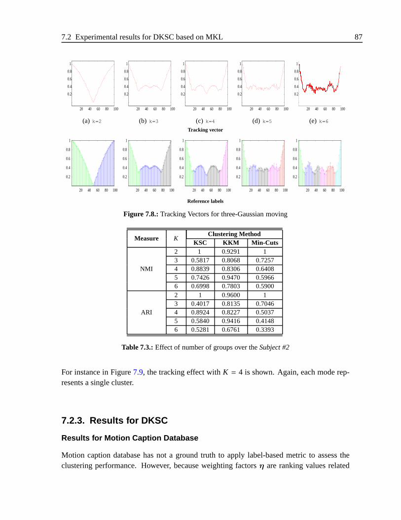
7.2 Experimental results for DKSC based on MKL 87
1
0.8
0.6
0.4
0.2
20 40 60 80 100
(a) k=2
1
0.8
0.6
0.4
0.2
20 40 60 80 100
(b) k=3
1
0.8
0.6
0.4
0.2
20 40 60 80 100
(c) k=4
1
0.8
0.6
0.4
0.2
20 40 60 80 100
(d) k=5
1
0.8
0.6
0.4
0.2
20 40 60 80 100
(e) k=6Tracking vector
1
0.8
0.6
0.4
0.2
20 40 60 80 100
1
0.8
0.6
0.4
0.2
20 40 60 80 100
1
0.8
0.6
0.4
0.2
20 40 60 80 100
1
0.8
0.6
0.4
0.2
20 40 60 80 100
1
0.8
0.6
0.4
0.2
20 40 60 80 100
Reference labels
Figure 7.8.:Tracking Vectors for three-Gaussian moving
Measure KClustering Method
KSC KKM Min-Cuts
NMI
2 1 0.9291 13 0.5817 0.8068 0.72574 0.8839 0.8306 0.64085 0.7426 0.9470 0.59666 0.6998 0.7803 0.5900
ARI
2 1 0.9600 13 0.4017 0.8135 0.70464 0.8924 0.8227 0.50375 0.5840 0.9416 0.41486 0.5281 0.6761 0.3393
Table 7.3.:Effect of number of groups over theSubject #2
For instance in Figure7.9, the tracking effect withK = 4 is shown. Again, each mode rep-resents a single cluster.
7.2.3. Results for DKSC
Results for Motion Caption Database
Motion caption database has not a ground truth to apply label-based metric to assess theclustering performance. However, because weighting factorsη are ranking values related
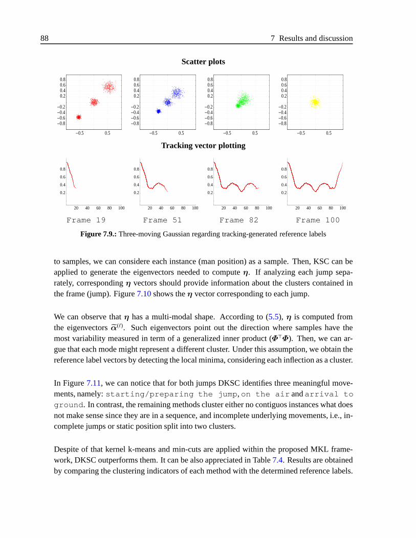
88 7 Results and discussion
Scatter plots
0.80.6
0.20.4
−0.8−0.6−0.4−0.2
0.5−0.5
40
0.80.6
0.20.4
−0.8−0.6−0.4−0.2
0.5−0.5
0.80.6
0.20.4
−0.8−0.6−0.4−0.2
0.5−0.5
0.80.6
0.20.4
−0.8−0.6−0.4−0.2
0.5−0.5
Tracking vector plotting
0.8
0.6
0.2
0.4
.5
20 40 60 80 100
0.8
0.6
0.2
0.4
20 40 60 80 100
0.8
0.6
0.2
0.4
20 40 60 80 100
0.8
0.6
0.2
0.4
20 40 60 80 100
Frame 19 Frame 51 Frame 82 Frame 100
Figure 7.9.:Three-moving Gaussian regarding tracking-generated reference labels
to samples, we can considere each instance (man position) as a sample. Then, KSC can beapplied to generate the eigenvectors needed to computeη. If analyzing each jump sepa-rately, correspondingη vectors should provide information about the clusters contained inthe frame (jump). Figure7.10shows theη vector corresponding to each jump.
We can observe thatη has a multi-modal shape. According to (5.5), η is computed fromthe eigenvectorsα(ℓ). Such eigenvectors point out the direction where samples have themost variability measured in term of a generalized inner product (Φ⊤Φ). Then, we can ar-gue that each mode might represent a different cluster. Under this assumption, we obtain thereference label vectors by detecting the local minima, considering each inflection as a cluster.
In Figure7.11, we can notice that for both jumps DKSC identifies three meaningful move-ments, namely:starting/preparing the jump,on the air andarrival to
ground. In contrast, the remaining methods cluster either no contiguos instances what doesnot make sense since they are in a sequence, and incomplete underlying movements, i.e., in-complete jumps or static position split into two clusters.
Despite of that kernel k-means and min-cuts are applied within the proposed MKL frame-work, DKSC outperforms them. It can be also appreciated in Table7.4. Results are obtainedby comparing the clustering indicators of each method with the determined reference labels.
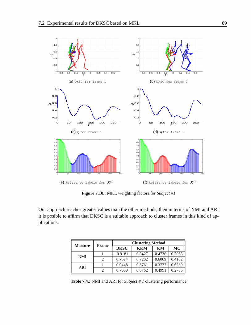
7.2 Experimental results for DKSC based on MKL 89
−0.8 −0.6 −0.4 −0.2 0 0.2 0.4 0.60
0.2
0.4
0.6
0.8
1
Y
Z
(a) DKSC for frame 1
−0.8 −0.6 −0.4 −0.2 0 0.2 0.4 0.60
0.2
0.4
0.6
0.8
1
Y
Z
(b) DKSC for frame 2
0 50 100 150 200 250
0.2
0.4
0.6
0.8
1
t
η t
(c) η for frame 1
0 50 100 150 200 250
0.2
0.4
0.6
0.8
1
t
η t(d) η for frame 2
0 50 100 150 200 250 3000
0.1
0.2
0.3
0.4
0.5
0.6
0.7
0.8
0.9
1
(e) Reference labels for X(1)
0 50 100 150 200 250 3000
0.1
0.2
0.3
0.4
0.5
0.6
0.7
0.8
0.9
1
(f) Reference labels for X(2)
Figure 7.10.:MKL weighting factors forSubject #1
Our approach reaches greater values than the other methods, then in terms of NMI and ARIit is posible to affirm that DKSC is a suitable approach to cluster frames in this kind of ap-plications.
Measure FrameClustering Method
DKSC KKM KM MC
NMI1 0.9181 0.8427 0.4736 0.70652 0.7624 0.7202 0.6009 0.4102
ARI1 0.9448 0.8761 0.3777 0.62392 0.7000 0.6762 0.4991 0.2755
Table 7.4.:NMI and ARI for Subject # 1clustering performance

90 7 Results and discussion
−0.8 −0.6 −0.4 −0.2 0 0.2 0.4 0.6 0.80
0.2
0.4
0.6
0.8
1
YZ
(a) DKSC
−0.8 −0.6 −0.4 −0.2 0 0.2 0.4 0.6 0.80
0.2
0.4
0.6
0.8
1
Y
Z
(b) KKM with MKL
−0.8 −0.6 −0.4 −0.2 0 0.2 0.4 0.6 0.80
0.2
0.4
0.6
0.8
1
Y
Z
(c) Min-Cuts with MKL
−0.8 −0.6 −0.4 −0.2 0 0.2 0.4 0.60
0.2
0.4
0.6
0.8
1
Y
Z
(d) KSC
−0.8 −0.6 −0.4 −0.2 0 0.2 0.4 0.60
0.2
0.4
0.6
0.8
1
Y
Z
(e) KM
Figure 7.11.:Clustering results forSubject #1
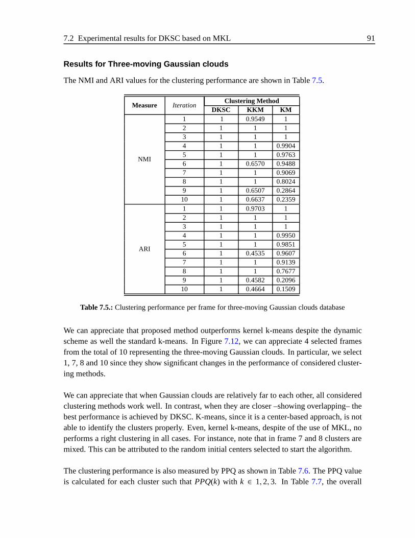
7.2 Experimental results for DKSC based on MKL 91
Results for Three-moving Gaussian clouds
The NMI and ARI values for the clustering performance are shown in Table7.5.
Measure IterationClustering Method
DKSC KKM KM
NMI
1 1 0.9549 12 1 1 13 1 1 14 1 1 0.99045 1 1 0.97636 1 0.6570 0.94887 1 1 0.90698 1 1 0.80249 1 0.6507 0.286410 1 0.6637 0.2359
ARI
1 1 0.9703 12 1 1 13 1 1 14 1 1 0.99505 1 1 0.98516 1 0.4535 0.96077 1 1 0.91398 1 1 0.76779 1 0.4582 0.209610 1 0.4664 0.1509
Table 7.5.:Clustering performance per frame for three-moving Gaussian clouds database
We can appreciate that proposed method outperforms kernel k-means despite the dynamicscheme as well the standard k-means. In Figure7.12, we can appreciate 4 selected framesfrom the total of 10 representing the three-moving Gaussian clouds. In particular, we select1, 7, 8 and 10 since they show significant changes in the performance of considered cluster-ing methods.
We can appreciate that when Gaussian clouds are relatively far to each other, all consideredclustering methods work well. In contrast, when they are closer –showing overlapping– thebest performance is achieved by DKSC. K-means, since it is a center-based approach, is notable to identify the clusters properly. Even, kernel k-means, despite of the use of MKL, noperforms a right clustering in all cases. For instance, note that in frame 7 and 8 clusters aremixed. This can be attributed to the random initial centers selected to start the algorithm.
The clustering performance is also measured by PPQ as shown in Table7.6. The PPQ valueis calculated for each cluster such thatPPQ(k) with k ∈ 1, 2, 3. In Table7.7, the overall

92 7 Results and discussion
results are presented –mean and standard deviation of the performance achieved by eachmethod per cluster. Once again, it can also be noticed that DKSC works the best in compar-ison with the other considered methods.
Albeit seeming that there is no a significant difference according the overall results, forframes 7, 8 and 9 the PPQ is considerably low for all methods excepting proposed DKSC.
IterationMethod PPQ(k) 1 2 3 4 5 6 7 8 9 10
KMk = 1 1 1 1 1 1 1 1 0.9852 0.7168 0.4338k = 2 1 1 1 0.995 0.9901 0.9217 0.8772 0.7658 0.5580 0.3462k = 3 1 1 1 0.995 0.9901 0.9217 0.8772 0.7707 0.5401 0.5176
DKKMk = 1 1 1 1 1 1 1 0.5 0.5 1 1k = 2 1 1 1 1 1 1 1 0.5 1 1k = 3 1 1 1 1 1 1 0.5 1 1 1
DKSCk = 1 1 1 1 1 1 1 1 1 1 1k = 2 1 1 1 1 1 1 1 1 1 1k = 3 1 1 1 1 1 1 1 1 1 1
Table 7.6.:Clusterings performance withPPQalong 10 iterations
PPQ(k)(µ ± σ)
Method k = 1 k = 2 k = 3KM 0.9136± 0.1904 0.8454± 0.2261 0.8612± 0.1902
DKKM 0.9± 0.2108 0.95± 0.1581 0.95± 0.1581DKSC 1± 0 1± 0 1± 0
Table 7.7.:Mean and standard deviation per cluster
It can also be noted in Figure7.12, where those frames perform a wrongly clustering. Then,among the considered methods, DKSC is the most suitable for this task because the matteris a time-varying framework and therefore during all the frame clustering must work well.
As a conclusion, we can say that our approach is an alternative to manage applications in-volving both hidden objects and dynamic data.
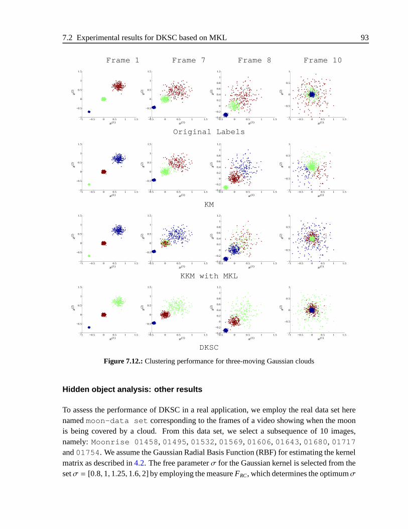
7.2 Experimental results for DKSC based on MKL 93
Frame 1 Frame 7 Frame 8 Frame 10
−1 −0.5 0 0.5 1 1.5−1
−0.5
0
0.5
1
1.5
x(1)
x(2
)
−0.5 0 0.5 1 1.5−1
−0.5
0
0.5
1
1.5
x(1)
x(2
)
−0.5 0 0.5 1 1.5−0.4
−0.2
0
0.2
0.4
0.6
0.8
1
1.2
x(1)
x(2
)
−1 −0.5 0 0.5 1 1.5−1
−0.5
0
0.5
1
x(1)
x(2
)
Original Labels
−1 −0.5 0 0.5 1 1.5−1
−0.5
0
0.5
1
1.5
x(1)
x(2
)
−0.5 0 0.5 1 1.5−1
−0.5
0
0.5
1
1.5
x(1)
x(2
)
−0.5 0 0.5 1 1.5−0.4
−0.2
0
0.2
0.4
0.6
0.8
1
1.2
x(1)
x(2
)
−1 −0.5 0 0.5 1 1.5−1
−0.5
0
0.5
1
x(1)
x(2
)
KM
−1 −0.5 0 0.5 1 1.5−1
−0.5
0
0.5
1
1.5
replacements
x(1)
x(2
)
−0.5 0 0.5 1 1.5−1
−0.5
0
0.5
1
1.5
x(1)
x(2
)
−0.5 0 0.5 1 1.5−0.4
−0.2
0
0.2
0.4
0.6
0.8
1
1.2
x(1)
x(2
)
−1 −0.5 0 0.5 1 1.5−1
−0.5
0
0.5
1
x(1)
x(2
)KKM with MKL
−1 −0.5 0 0.5 1 1.5−1
−0.5
0
0.5
1
1.5
x(1)
x(2
)
−0.5 0 0.5 1 1.5−1
−0.5
0
0.5
1
1.5
x(1)
x(2
)
−0.5 0 0.5 1 1.5−0.4
−0.2
0
0.2
0.4
0.6
0.8
1
1.2
x(1)
x(2
)
−1 −0.5 0 0.5 1 1.5−1
−0.5
0
0.5
1
x(1)
x(2
)
DKSC
Figure 7.12.:Clustering performance for three-moving Gaussian clouds
Hidden object analysis: other results
To assess the performance of DKSC in a real application, we employ the real data set herenamedmoon-data set corresponding to the frames of a video showing when the moonis being covered by a cloud. From this data set, we select a subsequence of 10 images,namely:Moonrise 01458, 01495, 01532, 01569, 01606, 01643, 01680, 01717and01754. We assume the Gaussian Radial Basis Function (RBF) for estimating the kernelmatrix as described in4.2. The free parameterσ for the Gaussian kernel is selected from thesetσ = [0.8, 1, 1.25, 1.6, 2] by employing the measureFRC, which determines the optimumσ
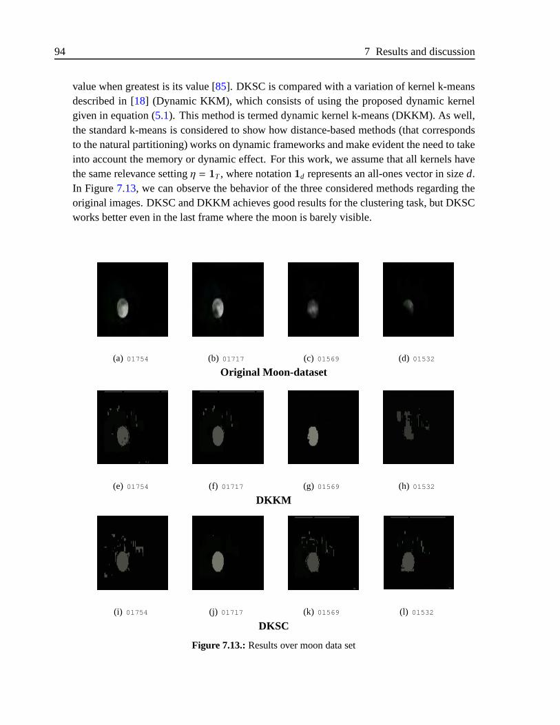
94 7 Results and discussion
value when greatest is its value [85]. DKSC is compared with a variation of kernel k-meansdescribed in [18] (Dynamic KKM), which consists of using the proposed dynamic kernelgiven in equation (5.1). This method is termed dynamic kernel k-means (DKKM). As well,the standard k-means is considered to show how distance-based methods (that correspondsto the natural partitioning) works on dynamic frameworks and make evident the need to takeinto account the memory or dynamic effect. For this work, we assume that all kernels havethe same relevance settingη = 1T , where notation1d represents an all-ones vector in sized.In Figure7.13, we can observe the behavior of the three considered methods regarding theoriginal images. DKSC and DKKM achieves good results for the clustering task, but DKSCworks better even in the last frame where the moon is barely visible.
(a) 01754 (b) 01717 (c) 01569 (d) 01532
Original Moon-dataset
(e) 01754 (f) 01717 (g) 01569 (h) 01532
DKKM
(i) 01754 (j) 01717 (k) 01569 (l) 01532
DKSC
Figure 7.13.:Results over moon data set
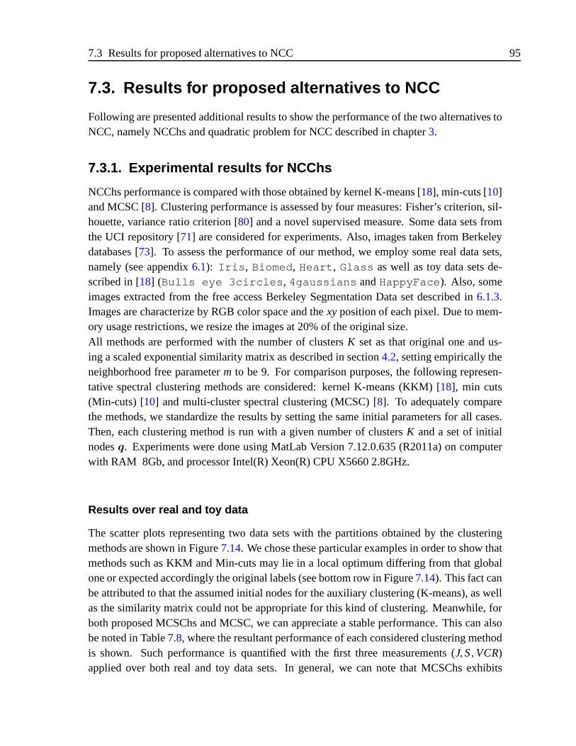
7.3 Results for proposed alternatives to NCC 95
7.3. Results for proposed alternatives to NCC
Following are presented additional results to show the performance of the two alternatives toNCC, namely NCChs and quadratic problem for NCC described in chapter3.
7.3.1. Experimental results for NCChs
NCChs performance is compared with those obtained by kernel K-means [18], min-cuts [10]and MCSC [8]. Clustering performance is assessed by four measures: Fisher’s criterion, sil-houette, variance ratio criterion [80] and a novel supervised measure. Some data sets fromthe UCI repository [71] are considered for experiments. Also, images taken from Berkeleydatabases [73]. To assess the performance of our method, we employ some real data sets,namely (see appendix6.1): Iris, Biomed, Heart, Glass as well as toy data sets de-scribed in [18] (Bulls eye 3circles, 4gaussians andHappyFace). Also, someimages extracted from the free access Berkeley Segmentation Data set described in6.1.3.Images are characterize by RGB color space and thexyposition of each pixel. Due to mem-ory usage restrictions, we resize the images at 20% of the original size.All methods are performed with the number of clustersK set as that original one and us-ing a scaled exponential similarity matrix as described in section4.2, setting empirically theneighborhood free parameterm to be 9. For comparison purposes, the following represen-tative spectral clustering methods are considered: kernel K-means (KKM) [18], min cuts(Min-cuts) [10] and multi-cluster spectral clustering (MCSC) [8]. To adequately comparethe methods, we standardize the results by setting the same initial parameters for all cases.Then, each clustering method is run with a given number of clustersK and a set of initialnodesq. Experiments were done using MatLab Version 7.12.0.635 (R2011a) on computerwith RAM 8Gb, and processor Intel(R) Xeon(R) CPU X5660 2.8GHz.
Results over real and toy data
The scatter plots representing two data sets with the partitions obtained by the clusteringmethods are shown in Figure7.14. We chose these particular examples in order to show thatmethods such as KKM and Min-cuts may lie in a local optimum differing from that globalone or expected accordingly the original labels (see bottom row in Figure7.14). This fact canbeattributed to that the assumed initial nodes for the auxiliary clustering (K-means), as wellas the similarity matrix could not be appropriate for this kind of clustering. Meanwhile, forboth proposed MCSChs and MCSC, we can appreciate a stable performance. This can alsobe noted in Table7.8, where the resultant performance of each considered clustering methodis shown. Such performance is quantified with the first three measurements (J,S,VCR)applied over both real and toy data sets. In general, we can note that MCSChs exhibits
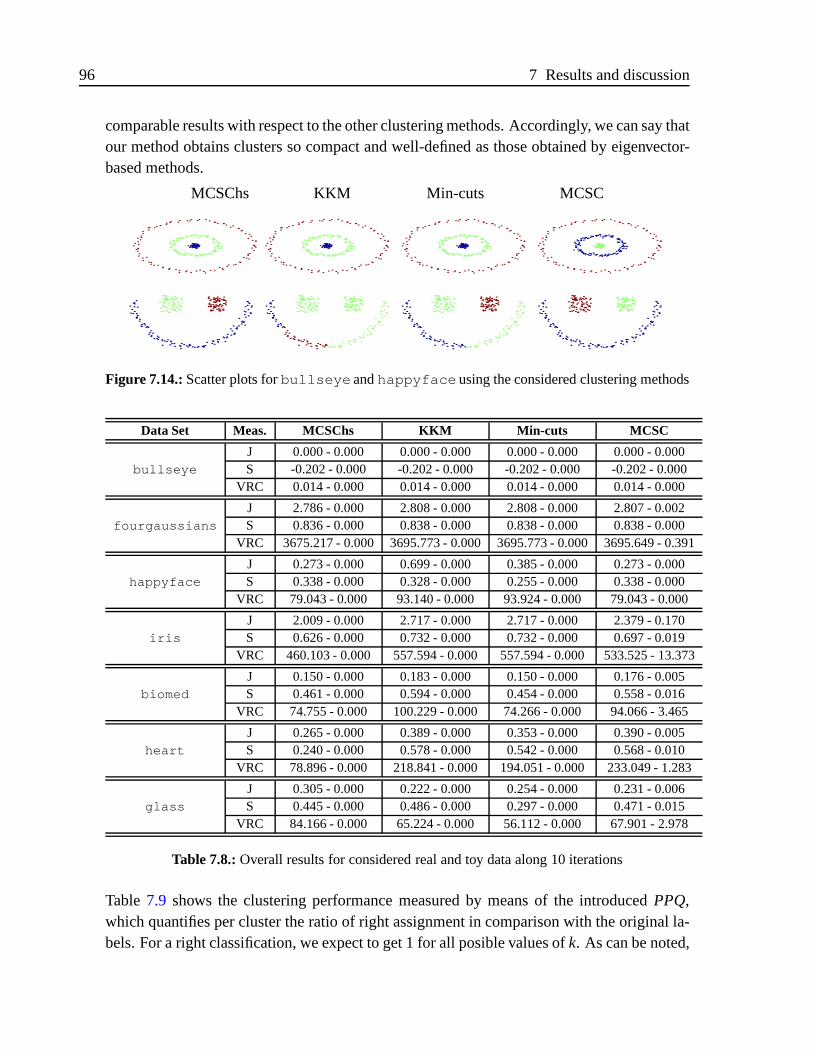
96 7 Results and discussion
comparable results with respect to the other clustering methods. Accordingly, we can say thatour method obtains clusters so compact and well-defined as those obtained by eigenvector-based methods.
MCSChs KKM Min-cuts MCSC
Figure 7.14.:Scatter plots forbullseye andhappyface using the considered clustering methods
Data Set Meas. MCSChs KKM Min-cuts MCSC
bullseyeJ 0.000 - 0.000 0.000 - 0.000 0.000 - 0.000 0.000 - 0.000S -0.202 - 0.000 -0.202 - 0.000 -0.202 - 0.000 -0.202 - 0.000
VRC 0.014 - 0.000 0.014 - 0.000 0.014 - 0.000 0.014 - 0.000
fourgaussiansJ 2.786 - 0.000 2.808 - 0.000 2.808 - 0.000 2.807 - 0.002S 0.836 - 0.000 0.838 - 0.000 0.838 - 0.000 0.838 - 0.000
VRC 3675.217 - 0.000 3695.773 - 0.000 3695.773 - 0.000 3695.649 - 0.391
happyfaceJ 0.273 - 0.000 0.699 - 0.000 0.385 - 0.000 0.273 - 0.000S 0.338 - 0.000 0.328 - 0.000 0.255 - 0.000 0.338 - 0.000
VRC 79.043 - 0.000 93.140 - 0.000 93.924 - 0.000 79.043 - 0.000
irisJ 2.009 - 0.000 2.717 - 0.000 2.717 - 0.000 2.379 - 0.170S 0.626 - 0.000 0.732 - 0.000 0.732 - 0.000 0.697 - 0.019
VRC 460.103 - 0.000 557.594 - 0.000 557.594 - 0.000 533.525 - 13.373
biomedJ 0.150 - 0.000 0.183 - 0.000 0.150 - 0.000 0.176 - 0.005S 0.461 - 0.000 0.594 - 0.000 0.454 - 0.000 0.558 - 0.016
VRC 74.755 - 0.000 100.229 - 0.000 74.266 - 0.000 94.066 - 3.465
heartJ 0.265 - 0.000 0.389 - 0.000 0.353 - 0.000 0.390 - 0.005S 0.240 - 0.000 0.578 - 0.000 0.542 - 0.000 0.568 - 0.010
VRC 78.896 - 0.000 218.841 - 0.000 194.051 - 0.000 233.049 - 1.283
glassJ 0.305 - 0.000 0.222 - 0.000 0.254 - 0.000 0.231 - 0.006S 0.445 - 0.000 0.486 - 0.000 0.297 - 0.000 0.471 - 0.015
VRC 84.166 - 0.000 65.224 - 0.000 56.112 - 0.000 67.901 - 2.978
Table 7.8.:Overall results for considered real and toy data along 10 iterations
Table 7.9 shows the clustering performance measured by means of the introducedPPQ,which quantifies per cluster the ratio of right assignment in comparison with the original la-bels. For a right classification, we expect to get 1 for all posible values ofk. As can be noted,
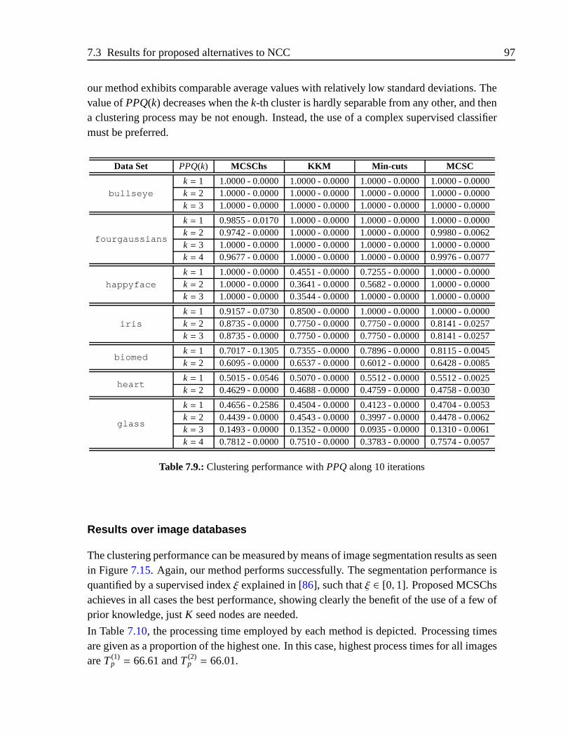
7.3 Results for proposed alternatives to NCC 97
our method exhibits comparable average values with relatively low standard deviations. Thevalue ofPPQ(k) decreases when thek-th cluster is hardly separable from any other, and thena clustering process may be not enough. Instead, the use of a complex supervised classifiermust be preferred.
Data Set PPQ(k) MCSChs KKM Min-cuts MCSC
bullseyek = 1 1.0000 - 0.0000 1.0000 - 0.0000 1.0000 - 0.0000 1.0000 - 0.0000k = 2 1.0000 - 0.0000 1.0000 - 0.0000 1.0000 - 0.0000 1.0000 - 0.0000k = 3 1.0000 - 0.0000 1.0000 - 0.0000 1.0000 - 0.0000 1.0000 - 0.0000
fourgaussians
k = 1 0.9855 - 0.0170 1.0000 - 0.0000 1.0000 - 0.0000 1.0000 - 0.0000k = 2 0.9742 - 0.0000 1.0000 - 0.0000 1.0000 - 0.0000 0.9980 - 0.0062k = 3 1.0000 - 0.0000 1.0000 - 0.0000 1.0000 - 0.0000 1.0000 - 0.0000k = 4 0.9677 - 0.0000 1.0000 - 0.0000 1.0000 - 0.0000 0.9976 - 0.0077
happyface
k = 1 1.0000 - 0.0000 0.4551 - 0.0000 0.7255 - 0.0000 1.0000 - 0.0000k = 2 1.0000 - 0.0000 0.3641 - 0.0000 0.5682 - 0.0000 1.0000 - 0.0000k = 3 1.0000 - 0.0000 0.3544 - 0.0000 1.0000 - 0.0000 1.0000 - 0.0000
iris
k = 1 0.9157 - 0.0730 0.8500 - 0.0000 1.0000 - 0.0000 1.0000 - 0.0000k = 2 0.8735 - 0.0000 0.7750 - 0.0000 0.7750 - 0.0000 0.8141 - 0.0257k = 3 0.8735 - 0.0000 0.7750 - 0.0000 0.7750 - 0.0000 0.8141 - 0.0257
biomedk = 1 0.7017 - 0.1305 0.7355 - 0.0000 0.7896 - 0.0000 0.8115 - 0.0045k = 2 0.6095 - 0.0000 0.6537 - 0.0000 0.6012 - 0.0000 0.6428 - 0.0085
heartk = 1 0.5015 - 0.0546 0.5070 - 0.0000 0.5512 - 0.0000 0.5512 - 0.0025k = 2 0.4629 - 0.0000 0.4688 - 0.0000 0.4759 - 0.0000 0.4758 - 0.0030
glass
k = 1 0.4656 - 0.2586 0.4504 - 0.0000 0.4123 - 0.0000 0.4704 - 0.0053k = 2 0.4439 - 0.0000 0.4543 - 0.0000 0.3997 - 0.0000 0.4478 - 0.0062k = 3 0.1493 - 0.0000 0.1352 - 0.0000 0.0935 - 0.0000 0.1310 - 0.0061k = 4 0.7812 - 0.0000 0.7510 - 0.0000 0.3783 - 0.0000 0.7574 - 0.0057
Table 7.9.:Clustering performance withPPQalong 10 iterations
Results over image databases
The clustering performance can be measured by means of image segmentation results as seenin Figure7.15. Again, our method performs successfully. The segmentation performance isquantified by a supervised indexξ explained in [86], such thatξ ∈ [0, 1]. Proposed MCSChsachieves in all cases the best performance, showing clearly the benefit of the use of a few ofprior knowledge, justK seed nodes are needed.
In Table7.10, the processing time employed by each method is depicted. Processing timesare given as a proportion of the highest one. In this case, highest process times for all imagesareT(1)
p = 66.61 andT(2)p = 66.01.
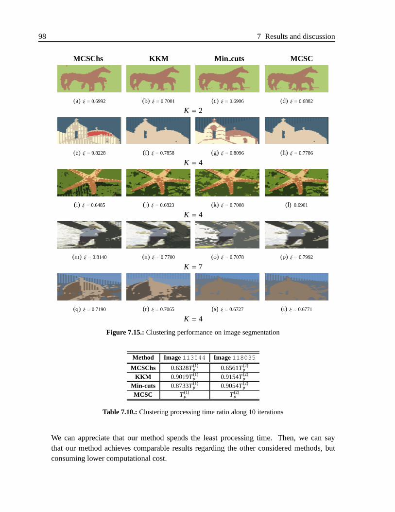
98 7 Results and discussion
MCSChs KKM Min cuts MCSC
(a) ξ = 0.6992 (b) ξ = 0.7001 (c) ξ = 0.6906 (d) ξ = 0.6882
K = 2
(e) ξ = 0.8228 (f) ξ = 0.7858 (g) ξ = 0.8096 (h) ξ = 0.7786
K = 4
(i) ξ = 0.6485 (j) ξ = 0.6823 (k) ξ = 0.7008 (l) 0.6901
K = 4
(m) ξ = 0.8140 (n) ξ = 0.7700 (o) ξ = 0.7078 (p) ξ = 0.7992
K = 7
(q) ξ = 0.7190 (r) ξ = 0.7065 (s) ξ = 0.6727 (t) ξ = 0.6771
K = 4
Figure 7.15.:Clustering performance on image segmentation
Method Image113044 Image118035
MCSChs 0.6328T(1)p 0.6561T(2)
p
KKM 0.9019T(1)p 0.9154T(2)
p
Min-cuts 0.8733T(1)p 0.9054T(2)
p
MCSC T(1)p T(2)
p
Table 7.10.:Clustering processing time ratio along 10 iterations
We can appreciate that our method spends the least processing time. Then, we can saythat our method achieves comparable results regarding the other considered methods, butconsuming lower computational cost.
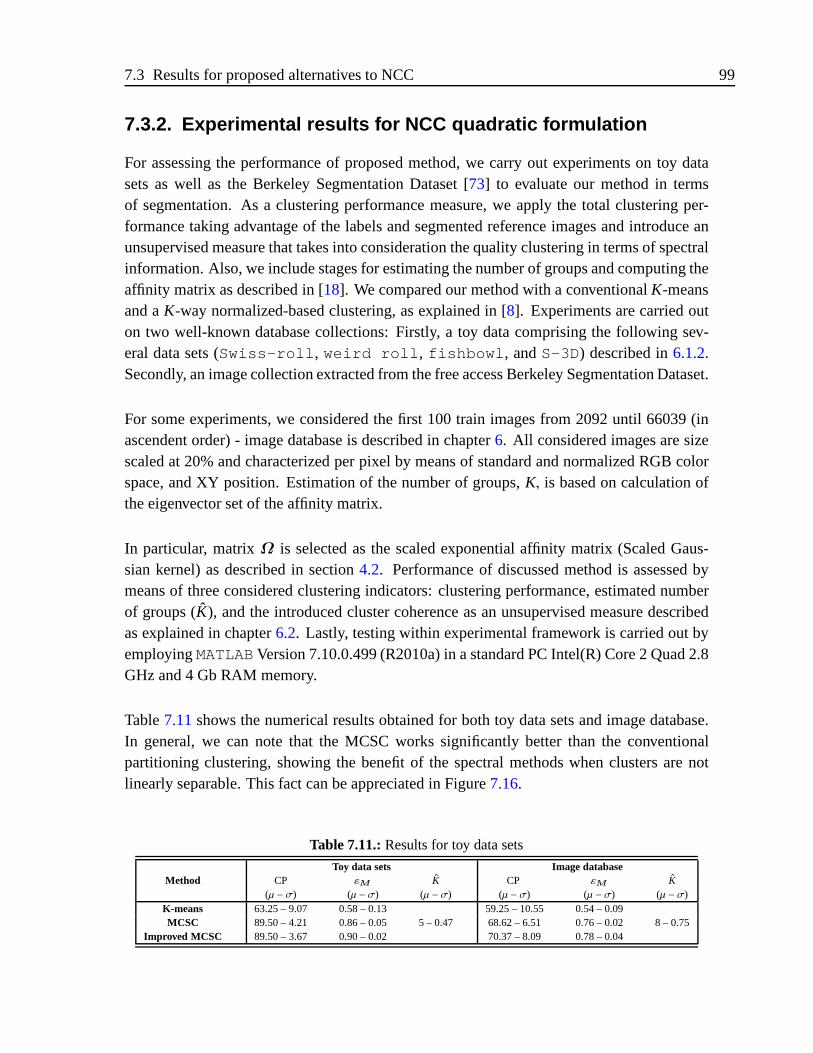
7.3 Results for proposed alternatives to NCC 99
7.3.2. Experimental results for NCC quadratic formulation
For assessing the performance of proposed method, we carry out experiments on toy datasets as well as the Berkeley Segmentation Dataset [73] to evaluate our method in termsof segmentation. As a clustering performance measure, we apply the total clustering per-formance taking advantage of the labels and segmented reference images and introduce anunsupervised measure that takes into consideration the quality clustering in terms of spectralinformation. Also, we include stages for estimating the number of groups and computing theaffinity matrix as described in [18]. We compared our method with a conventionalK-meansand aK-way normalized-based clustering, as explained in [8]. Experiments are carried outon two well-known database collections: Firstly, a toy data comprising the following sev-eral data sets (Swiss-roll, weird roll, fishbowl, andS-3D) described in6.1.2.Secondly, an image collection extracted from the free access Berkeley Segmentation Dataset.
For some experiments, we considered the first 100 train images from 2092 until 66039 (inascendent order) - image database is described in chapter6. All considered images are sizescaled at 20% and characterized per pixel by means of standard and normalized RGB colorspace, and XY position. Estimation of the number of groups,K, is based on calculation ofthe eigenvector set of the affinity matrix.
In particular, matrixΩ is selected as the scaled exponential affinity matrix (Scaled Gaus-sian kernel) as described in section4.2. Performance of discussed method is assessed bymeans of three considered clustering indicators: clustering performance, estimated numberof groups (K), and the introduced cluster coherence as an unsupervised measure describedas explained in chapter6.2. Lastly, testing within experimental framework is carried out byemployingMATLAB Version 7.10.0.499 (R2010a) in a standard PC Intel(R) Core 2 Quad 2.8GHz and 4 Gb RAM memory.
Table7.11shows the numerical results obtained for both toy data sets andimage database.In general, we can note that the MCSC works significantly better than the conventionalpartitioning clustering, showing the benefit of the spectral methods when clusters are notlinearly separable. This fact can be appreciated in Figure7.16.
Table 7.11.:Results for toy data sets
Toy data sets Image databaseMethod CP εM K CP εM K
(µ − σ) (µ − σ) (µ − σ) (µ − σ) (µ − σ) (µ − σ)K-means 63.25 – 9.07 0.58 – 0.13 59.25 – 10.55 0.54 – 0.09MCSC 89.50 – 4.21 0.86 – 0.05 5 – 0.47 68.62 – 6.51 0.76 – 0.02 8 – 0.75
Improved MCSC 89.50 – 3.67 0.90 – 0.02 70.37 – 8.09 0.78 – 0.04
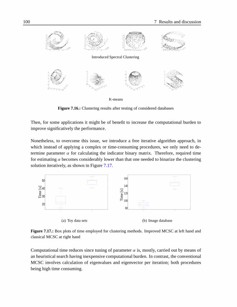
100 7 Results and discussion
Introduced Spectral Clustering
K-means
Figure 7.16.:Clustering results after testing of considered databases
Then, for some applications it might be of benefit to increase the computational burden toimprove significatively the performance.
Nonetheless, to overcome this issue, we introduce a free iterative algorithm approach, inwhich instead of applying a complex or time-consuming procedures, we only need to de-termine parameterα for calculating the indicator binary matrix. Therefore, required timefor estimatingα becomes considerably lower than that one needed to binarize the clusteringsolution iteratively, as shown in Figure7.17.
20
30
40
50
1 2
Tim
e[s
]
(a) Toy data sets
80
100
120
140
160
1 2
Tim
e[s
]
(b) Image database
Figure 7.17.:Box plots of time employed for clustering methods. Improved MCSC at left hand andclassical MCSC at right hand
Computational time reduces since tuning of parameterα is, mostly, carried out by means ofan heuristical search having inexpensive computational burden. In contrast, the conventionalMCSC involves calculation of eigenvalues and eigenvector per iteration; both proceduresbeing high time consuming.
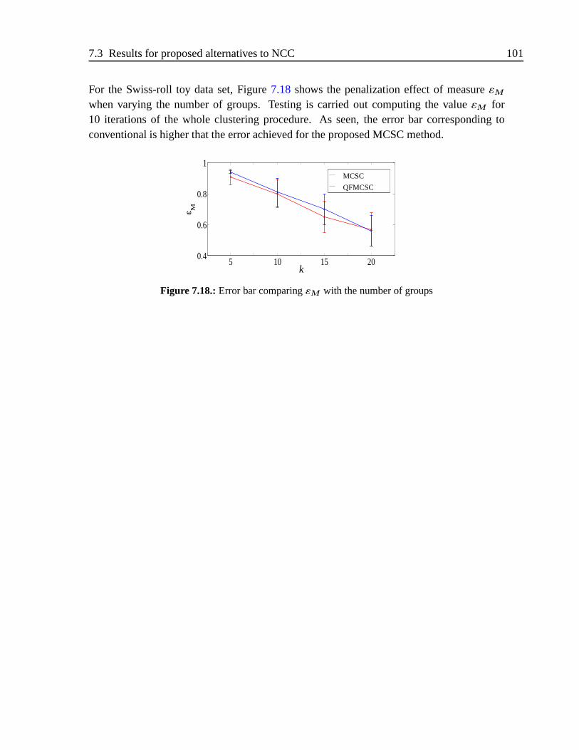
7.3 Results for proposed alternatives to NCC 101
For the Swiss-roll toy data set, Figure7.18 shows the penalization effect of measureεMwhen varying the number of groups. Testing is carried out computing the valueεM for10 iterations of the whole clustering procedure. As seen, the error bar corresponding toconventional is higher that the error achieved for the proposed MCSC method.
5 10 15 200.4
0.6
0.8
1
ε M
k
MCSC
QFMCSC
Figure 7.18.:Error bar comparingεM with the number of groups

Part IV.
Final remarks
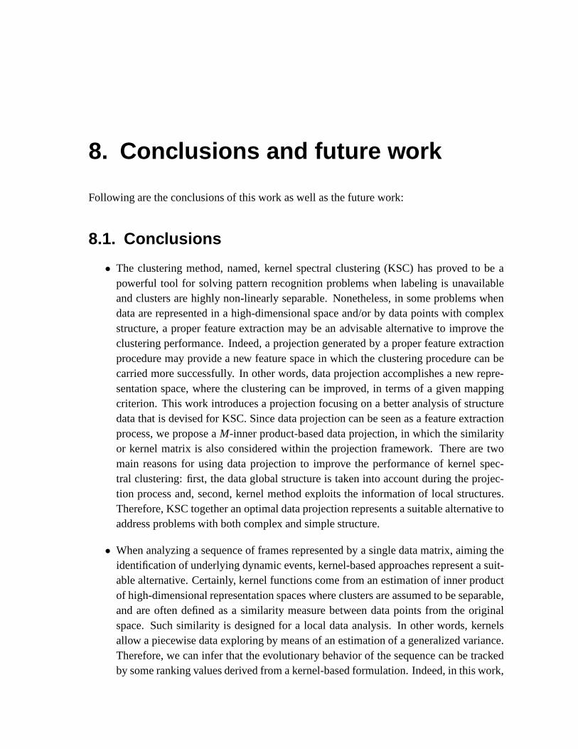
8. Conclusions and future work
Following are the conclusions of this work as well as the future work:
8.1. Conclusions
• The clustering method, named, kernel spectral clustering (KSC) has proved to be apowerful tool for solving pattern recognition problems when labeling is unavailableand clusters are highly non-linearly separable. Nonetheless, in some problems whendata are represented in a high-dimensional space and/or by data points with complexstructure, a proper feature extraction may be an advisable alternative to improve theclustering performance. Indeed, a projection generated by a proper feature extractionprocedure may provide a new feature space in which the clustering procedure can becarried more successfully. In other words, data projection accomplishes a new repre-sentation space, where the clustering can be improved, in terms of a given mappingcriterion. This work introduces a projection focusing on a better analysis of structuredata that is devised for KSC. Since data projection can be seen as a feature extractionprocess, we propose aM-inner product-based data projection, in which the similarityor kernel matrix is also considered within the projection framework. There are twomain reasons for using data projection to improve the performance of kernel spec-tral clustering: first, the data global structure is taken into account during the projec-tion process and, second, kernel method exploits the information of local structures.Therefore, KSC together an optimal data projection represents a suitable alternative toaddress problems with both complex and simple structure.
• When analyzing a sequence of frames represented by a single data matrix, aiming theidentification of underlying dynamic events, kernel-based approaches represent a suit-able alternative. Certainly, kernel functions come from an estimation of inner productof high-dimensional representation spaces where clusters are assumed to be separable,and are often defined as a similarity measure between data points from the originalspace. Such similarity is designed for a local data analysis. In other words, kernelsallow a piecewise data exploring by means of an estimation of a generalized variance.Therefore, we can infer that the evolutionary behavior of the sequence can be trackedby some ranking values derived from a kernel-based formulation. Indeed, in this work,

104 8 Conclusions and future work
we demonstrate that a feasible tracking approach can be accomplished by maximiz-ing an energy term regarding an approximated version of the high-dimensional repre-sentation space. We use a linear orthonormal model, being the aim of maximizationproblem the calculation of an optimal low rank projection or rotation matrix. Finally,taking advantage of the singular value decomposition of kernel matrix, we deduce atracking vector as a linear combination of the squared eigenvectors. Tracking is doneaimed to find an unique value representing adequately each single frame. The hereproposed tracking approach determines a vector that has a direct relationship with theunderlying dynamic behavior of the analyzed sequence, allowing even to estimate thenumber of groups as well as the ground truth.
• Under the premise that a set of different kernels may represent more properly the in-put data than a single kernel, it has arisen the multiple kernel learning (MKL). Inother words, a suitable alternative to analyze and explore data can be posed within aMKL framework. MKL has emerged to deal with different issues in machine learning,mainly, regarding support vector machines. The intuitive idea of MKL is that learningcan be enhanced when using simultaneously different kernels. Indeed, local analysisprovided by each kernel helps to exploring the structure of the whole data when hav-ing local complex clusters. In this work, within a MKL framework, a dynamic kernelspectral clustering (DKSC) approach is introduced. MKL is used in such a mannerthat kernel matrices are computed from an input data sequence, in which each datamatrix represents a frame at a different time instance. Afterwards, a cumulative ker-nel is calculated as a linear combination of the previously obtained kernels where theweighting factors are obtained by ranking each sample contained in the frame. Suchranking corresponds to a tracking vector. Finally, data are clustered using the cumu-lative kernel matrix. As a conclusion, we can say that a linear combination of kernelsis an alternative to cluster dynamic data taking into account past information, wherecoefficients or weighting factors can be obtained from an eigenvector-based problem.Also, we verified that there exists a direct relationship between the weighting factorsand the supposed ground truth.
8.2. Future work
• New optimal projections in terms of different clustering criteria are to be considered.For instance, by searching optimal basis generated by the eigenvector decompositions.Likewise, other properties of spectral clustering algorithms should be explored to de-velop a method less sensitive to initialization, which enhances the trade-off betweenaccuracy and processing speed.
• Aiming to design an accurate tracking method able to be extended to prediction prob-
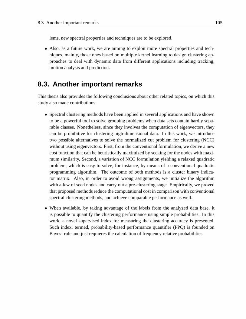
8.3 Another important remarks 105
lems, new spectral properties and techniques are to be explored.
• Also, as a future work, we are aiming to exploit more spectral properties and tech-niques, mainly, those ones based on multiple kernel learning to design clustering ap-proaches to deal with dynamic data from different applications including tracking,motion analysis and prediction.
8.3. Another important remarks
This thesis also provides the following conclusions about other related topics, on which thisstudy also made contributions:
• Spectral clustering methods have been applied in several applications and have shownto be a powerful tool to solve grouping problems when data sets contain hardly sepa-rable classes. Nonetheless, since they involves the computation of eigenvectors, theycan be prohibitive for clustering high-dimensional data. In this work, we introducetwo possible alternatives to solve the normalized cut problem for clustering (NCC)without using eigenvectors. First, from the conventional formulation, we derive a newcost function that can be heuristically maximized by seeking for the nodes with maxi-mum similarity. Second, a variation of NCC formulation yielding a relaxed quadraticproblem, which is easy to solve, for instance, by means of a conventional quadraticprogramming algorithm. The outcome of both methods is a cluster binary indica-tor matrix. Also, in order to avoid wrong assignments, we initialize the algorithmwith a few of seed nodes and carry out a pre-clustering stage. Empirically, we provedthat proposed methods reduce the computational cost in comparison with conventionalspectral clustering methods, and achieve comparable performance as well.
• When available, by taking advantage of the labels from the analyzed data base, itis possible to quantify the clustering performance using simple probabilities. In thiswork, a novel supervised index for measuring the clustering accuracy is presented.Such index, termed, probability-based performance quantifier (PPQ) is founded onBayes’ rule and just requieres the calculation of frequency relative probabilities.

Part V.
Appendixes
A. Kernel K-means
Kernel K-means method is a generalization of standard K-means that can be seen as aspectral relaxation [87]. As discussed before, spectral clustering approaches usually areperformed on a lower-dimensional space, keeping the pairwise relationships among nodes.Then, it often leads to a relaxed NP-problems where continuous solutions are obtained bya eigen-decomposition. Such a eigen-decomposition is regarding the normalized similaritymatrix (Laplacian, as well). In a Kernel K-means framework, eigenvectors are considered asgeometric coordinates and then K-means methods is applied over the eigen-space toget theresultant clusters [18,32]. In FigureA.1, a graphic explanation of Kernel K-means is shownthat depicts an instance of image segmentation procedure.
Image
I ∈ Rm×n X ∈ RN×d
Input Data
xx
xx
xx
N = mnd: Number of features
Eigenspace
xx
x
Kmeans
xx
x
V = eig(P)V ∈ RN×N
P :kernel matrix
q = kmeans(V ,K)K: Number of groupsq: cluster assignment
Figure A.1.: Graphically explanation of Kernel K-means for pixel clustering oriented to image seg-mentation
Previous instance is as follows: Suppose that we have a gray scale matrixm× n pixels insize. Characterizing each image pixel withd features -e. g., color spaces, morphologicaldescriptors- it is yielded as a result a data matrix in the formX ∈ RN×d, whereN = mn.Afterwards, the eigenvectorsV RN×N of a normalized kernel matrixP ∈ RN×N such thatP = D−1Ω, beingΩ the kernel matrix andD ∈ RN×N the corresponding degree matrix.Then, we proceed to clusterV into K groups using K-means algorithm:q = kmeans(V ,K),beingq ∈ RN the output cluster indicator such thatqi ∈ [K]. The segmented image is then am× n sized matrix holding regions in accordance withq.
B. Links with normalized cutclustering
This appendix deals with the relationship between KSC and NCC, starting from the formu-lation of the NC problem until reaching a WPCA formulation in a finite domain.
B.1. Multi-cluster spectral clustering (MCSC) fromtwo point of view
Recalling the formulation of MCSC given in chapter3, the well-known K-way normalizedcut-based clustering can be written as:
max1K
tr(M⊤ΩM )
tr(M⊤DM )= max
m(k)
1K
∑Kk=1 m
(k)⊤Ωm(k)
∑Kk=1 m
⊤m(B.1a)
s. t. M ∈ 0, 1N×K, M1K = 1N (B.1b)
Expressions (C.1a) and (C.1b) are the formulation of the NC optimization problem, named(NCPM). Previous formulation can also be expressed as follows. LetΩ = D−1/2
ΩD−1/2 bea normalized kernel matrix andL = D1/2M be a binary matrix normalized by the squareroot of the kernel degree. Then, a newNCPMversion can be expressed as:
maxL
1K
tr(L⊤ΩL)tr(L⊤L)
= maxℓ(k)
1K
∑Kk=1 ℓ
(k)⊤Ωℓ(k)
∑Kk=1 ℓ
(k)⊤ℓ(k)(B.2a)
s. t. D−1/2L ∈ 0, 1N×K, D−1/2L1K = 1N (B.2b)
whereℓ(k) is the columnk of L.
Solution of former problem has been addressed in [8,15] by introducing a relaxed version,in which numerator is maximized subject to denominator is constant, so
maxL
1K
tr(L⊤ΩL) s. t. tr(L⊤L) = const. (B.3)
Indeed, authors assume the particular caseL⊤L = IK, i.e. lettingL be an orthonormal ma-trix. Then, solution correspond to anyK-dimensional basis of normalized matrix eigenvec-tors. Despite that in [15] it is presented an one-iteration solution forNCPM with suboptimal
B.2 Solving the problem by a difference: Empirical feature map 109
results avoiding the calculation of SVD per iteration, the omitting of the effect of denomina-tor tr(L⊤L) by assuming orthogonality causes that the solution cannot be guaranteed to bea global optimum. In addition, this kind of formulation provide non-stable solutions due tothe heuristic search carried out to determine an optimal rotation matrix [15].
B.2. Solving the problem by a difference: Empiricalfeature map
Recalling original problemC.1, we introduce another way to solve theNCPM formula-tion via a minimization problem where the aims for maximizing tr(L⊤ΩL) and minimizingtr(L⊤L) can be accomplished simultaneously, so:
maxL
tr(L⊤ΩL Diag(γ)) − tr(L⊤L) (B.4)
whereγ = (γ1, . . . , γN)⊤ is a vector containing the regularization parameters.Let us assumeΩ = ΨΨ
⊤ whereΨ is a N × N dimensional auxiliary matrix, and considerthe following equality:
tr(Ω) = tr(D−1/2ΩD−1/2) = tr(D−1
Ω) = tr(D−1ΨΨ
⊤) = tr(Ψ⊤D−1Ψ)
then
D−1/2ΩD−1/2
= Ψ⊤D−1
Ψ
Previous formulation is possible since kernel matrixΩ is symmetric. Now, let us defineh(k) ∈ RN
= Ψ⊤ℓ(k) as thek-th projection andH = (h(1), · · · ,h(K)) as the projections matrix.
Then, formulation given by (C.4) can be expressed as follows:
maxh(k),ℓ(k),γk
12K
K∑
k=1
γkh(k)⊤V h(k) − 1
2
K∑
k=1
ℓ(k)⊤ℓ(k) (B.5a)
such thath(k)= Ψℓ(k) (B.5b)
where matrixV ∈ RN×N can be chosen as:
- IN: We can normalize matrixΩ in such way for alli condition∑N
j ωi j = 1 is satisfiedand therefore we would obtain a degree matrix equaling the identity matrix. Then,∑h(l)⊤h(l)
= tr(H⊤H), which corresponds to a PCA-based formulation.
- Diag(v): With v ∈ RN such thatv⊤v = 1, we have a WPCA approach.
- D−1: Given the equalityV = D−1, optimization problem can be solved by means of aprocedure based on random walks; being the case of interest in this study.
110 B Links with normalized cut clustering
B.2.1. Gaussian processes
In terms of Gaussian processes, variableΨ represents a mapping matrix such thatΨ =
(ψ(x1), . . . , ψ(xN)) and whereψ(·) : Rd → RN) is mapping function, which provides a newN-dimensional data representation where resultant clusters are assumed to be more sepa-rable. Also, matrixΩ is to be chosen as a Gaussian kernel [88]. Therefore, according tooptimization problem given by (C.5), termh(k) is to be thek-th projection of normalizedbinary indicators ash(k)
= Ψℓ(k).
B.2.2. Eigen-solution
We present a solution forC.5, which after solving the KKT conditions on its correspondingLagrangian, an eigenvectors problem is yielded. Then, we first solve the Lagrangian ofproblem (C.5) so:
L(h, ℓ, γ,α) =1
2Kh⊤V h − 1
2ℓ⊤ℓ −α⊤(h −Ψw) (B.6)
whereα is aN-dimensional vector containing the Lagrange multipliers.
Solving the partial derivatives to determine the KKT conditions, we have.
∂L
∂h= 0 ⇒ h =
KγDα
∂L
∂ℓ= 0 ⇒ ℓ = Ψ
⊤α
∂L
∂α= 0 ⇒ h = Ψℓ
Eliminating the primal variables, we obtain the following eigenvector problem:
λα =D−1Ωα (B.7)
whereλ = N/γ. Then, matrix∆K = (α(1), · · · ,α(K)) can be computed as the eigenvectorsassociated with the firstK longest eigenvalues ofD−1
Ω.
Finally, projections matrixH is in the form
H = ΨL = ΨD1/2M = Ω∆K (B.8)
and thereforeM = Ψ−1D−1/2
Ω∆K, whereΨ can be obtained from a Cholesky decomposi-tion.
C. Links between KSC withnormalized cut clustering
This chapter deals with the relationship between KSC and NCC, starting from the formula-tion of the NC problem until reaching a WPCA formulation in a finite domain.
C.1. Multi-cluster spectral clustering (MCSC) fromtwo point of view
Recalling the formulation of MCSC given in chapter3, the well-known K-way normalizedcut-based clustering can be written as:
max1K
tr(M⊤ΩM )
tr(M⊤DM )= max
m(k)
1K
∑Kk=1 m
(k)⊤Ωm(k)
∑Kk=1 m
⊤m(C.1a)
s. t. M ∈ 0, 1N×K, M1K = 1N (C.1b)
Expressions (C.1a) and (C.1b) are the formulation of the NC optimization problem, named(NCPM). Previous formulation can also be expressed as follows. LetΩ = D−1/2
ΩD−1/2 bea normalized kernel matrix andL = D1/2M be a binary matrix normalized by the squareroot of the kernel degree. Then, a newNCPMversion can be expressed as:
maxL
1K
tr(L⊤ΩL)tr(L⊤L)
= maxℓ(k)
1K
∑Kk=1 ℓ
(k)⊤Ωℓ(k)
∑Kk=1 ℓ
(k)⊤ℓ(k)(C.2a)
s. t. D−1/2L ∈ 0, 1N×K, D−1/2L1K = 1N (C.2b)
whereℓ(k) is the columnk of L.
Solution of former problem has been addressed in [8,15] by introducing a relaxed version,in which numerator is maximized subject to denominator is constant, so
maxL
1K
tr(L⊤ΩL) s. t. tr(L⊤L) = const. (C.3)
Indeed, authors assume the particular caseL⊤L = IK, i.e. lettingL be an orthonormal ma-trix. Then, solution correspond to anyK-dimensional basis of normalized matrix eigenvec-tors. Despite that in [15] it is presented an one-iteration solution forNCPM with suboptimal
112 C Links between KSC with normalized cut clustering
results avoiding the calculation of SVD per iteration, the omitting of the effect of denomina-tor tr(L⊤L) by assuming orthogonality causes that the solution cannot be guaranteed to bea global optimum. In addition, this kind of formulation provide non-stable solutions due tothe heuristic search carried out to determine an optimal rotation matrix [15].
C.2. Solving the problem by a difference: Empiricalfeature map
Recalling original problemC.1, we introduce another way to solve theNCPM formula-tion via a minimization problem where the aims for maximizing tr(L⊤ΩL) and minimizingtr(L⊤L) can be accomplished simultaneously, so:
maxL
tr(L⊤ΩL Diag(γ)) − tr(L⊤L) (C.4)
whereγ = (γ1, . . . , γN)⊤ is a vector containing the regularization parameters.Let us assumeΩ = ΨΨ
⊤ whereΨ is a N × N dimensional auxiliary matrix, and considerthe following equality:
tr(Ω) = tr(D−1/2ΩD−1/2) = tr(D−1
Ω) = tr(D−1ΨΨ
⊤) = tr(Ψ⊤D−1Ψ)
then
D−1/2ΩD−1/2
= Ψ⊤D−1
Ψ
Previous formulation is possible since kernel matrixΩ is symmetric. Now, let us defineh(k) ∈ RN
= Ψ⊤ℓ(k) as thek-th projection andH = (h(1), · · · ,h(K)) as the projections matrix.
Then, formulation given by (C.4) can be expressed as follows:
maxh(k),ℓ(k),γk
12K
K∑
k=1
γkh(k)⊤V h(k) − 1
2
K∑
k=1
ℓ(k)⊤ℓ(k) (C.5a)
such thath(k)= Ψℓ(k) (C.5b)
where matrixV ∈ RN×N can be chosen as:
- IN: We can normalize matrixΩ in such way for alli condition∑N
j ωi j = 1 is satisfiedand therefore we would obtain a degree matrix equaling the identity matrix. Then,∑h(l)⊤h(l)
= tr(H⊤H), which corresponds to a PCA-based formulation.
- Diag(v): With v ∈ RN such thatv⊤v = 1, we have a WPCA approach.
- D−1: Given the equalityV = D−1, optimization problem can be solved by means of aprocedure based on random walks; being the case of interest in this study.
C.2 Solving the problem by a difference: Empirical feature map 113
C.2.1. Gaussian processes
In terms of Gaussian processes, variableΨ represents a mapping matrix such thatΨ =
(ψ(x1), . . . , ψ(xN)) and whereψ(·) : Rd → RN) is mapping function, which provides a newN-dimensional data representation where resultant clusters are assumed to be more sepa-rable. Also, matrixΩ is to be chosen as a Gaussian kernel [88]. Therefore, according tooptimization problem given by (C.5), termh(k) is to be thek-th projection of normalizedbinary indicators ash(k)
= Ψℓ(k).
C.2.2. Eigen-solution
We present a solution forC.5, which after solving the KKT conditions on its correspondingLagrangian, an eigenvectors problem is yielded. Then, we first solve the Lagrangian ofproblem (C.5) so:
L(h, ℓ, γ,α) =1
2Kh⊤V h − 1
2ℓ⊤ℓ −α⊤(h −Ψw) (C.6)
whereα is aN-dimensional vector containing the Lagrange multipliers.
Solving the partial derivatives to determine the KKT conditions, we have.
∂L
∂h= 0 ⇒ h =
KγDα
∂L
∂ℓ= 0 ⇒ ℓ = Ψ
⊤α
∂L
∂α= 0 ⇒ h = Ψℓ
Eliminating the primal variables, we obtain the following eigenvector problem:
λα =D−1Ωα (C.7)
whereλ = N/γ. Then, matrix∆K = (α(1), · · · ,α(K)) can be computed as the eigenvectorsassociated with the firstK longest eigenvalues ofD−1
Ω.
Finally, projections matrixH is in the form
H = ΨL = ΨD1/2M = Ω∆K (C.8)
and thereforeM = Ψ−1D−1/2
Ω∆K, whereΨ can be obtained from a Cholesky decomposi-tion.

D. Relevance Analysis for featureextraction and selection viaspectral analysis
This appendix explains a relevance analysis approach, which is aimed to ranking variables orfeatures solving a feature extraction problem by determining an optimal data representation.In this case, such data representation is a linear combination of input features. The statementspresented here complement the explanation of the tracking approach and the WPCA-basedclustering described in chapter5 and4, respectively.
For further statements consider the notation given in TableD.1.
Term Notation Description
Original data matrix X X ∈ RN×d
Rotation matrix V V ∈ Rd×d, V TV = Id
Truncated rotation matrix V V ∈ Rd×p, V TV = Ip
Projected data Y Y ∈ RN×d,Y =XV
Truncated projected data Y Y ∈ RN×p, Y = XV
Reconstructed data X X ∈ RN×d, X = Y V T
Table D.1.:Notation used throughout this chapter
The purpose of this approach is to determine weighting factors for variables in order to carryout either a proper dimensionality reduction or feature extraction. LetX ∈ RN×d be thefeature or data matrix being centered i.e with zero mean regarding its columns. Then, wecan extract features by means of a linear combination of input feature via the linear projectionmatrixY ∈ RN×d defined as:
Y =XV ,
beingV ∈ Rd×d an orthogonal matrix. Generally, the projection is performed over a lowerdimensional space, which means means that data are projected with a low-rank representa-tion of rotation matrixV ∈ Rd×p beingp < d. Therefore, a truncated projected data matrix
D.1 Feature relevance 115
Y ∈ RN×p can be written as:
Y =XV . (D.1)
Likewise, a lower-rank data matrixX ∈ RN×d can be obtained by reconstructing the datamatrix usingV instead of the whole orthonormal base. Then, from equationD.1, we havethat
X = Y V T. (D.2)
To quantify how accurately the truncated matrix representX, an error functionǫ(·, ·) is used.This function can be assumed as a distance measure betweenX andX such that
ǫ(X , X) = d(X , X), (D.3)
where d(·, ·) represents an assumed distance operator.
Let W ∈ Rd×d a diagonal weighting matrix defined asW = diag(√w), wherew =
[w1, . . . ,wd] is the weighting factor vector. Then, the weighted data matrixX ∈ RN×d canbe expressed asX = XW . From the weighted data matrix, we can define the weightingcovariance matrix (sample wise)ΣX ∈ Rd×d [89] as follows:
ΣX = XTX =W TXTXW .
D.1. Feature relevance
Relevance analysis distinguish those features that best represent determined input data and/ormost contribute to effectively discriminate among the disjoint data subsets into the wholeinput data. Such features are named asrelevant features. Thus, it also recognize featureswhose representation or discrimination capability is low, namedirrelevant features); as wellas those that have repeated information (redundant features).A data matrixX ∈ RN×d comprisingN data points or samples described by ad-dimensionalfeature setx(1), . . . ,x(d), wherex(ℓ) is the columnd of data matrix. To represent eachfeature, consider the indexξℓ and then the whole feature set is represented byξ = ξ1, . . . , ξd.Besides, each sample is associated to one, and only one, element from the class label setc = ck ∈ N : k = 1, . . . ,K, , whereK is the number of data subsets. Then, for each one ofthe featuresξℓ ∈ ξ, the relevance functiong is defined as follows:
g : RN×d × R → R+
(Xξ, ξℓ) 7→ g(Xξ, ξℓ) (D.4)
116 D Relevance Analysis for feature extraction and selectionvia spectral analysis
such thatg(Xξ, ξi) is higher when the relevance ofℓ-th feature is greater.
In other words, the aim of relevance analysis is to find out a low-dimensional and compactrepresentation of data that preserves the most relevant information of the original observationspace according to a given relevance measureg. To that end, it is commonly applied a cri-terion which relate the original and truncated matriz and can be expressed asε = φ(X , X).Commonly, this criterion is based on distances. In that case, there exist several alternativesfor calculating this distance, such as, the Minkowski distance (Lp metrics), square Euclideandistance, angle–based distance, Mahalanobis, among others, as discussed in [90]. In general,analysis of relevance methods aim to minimizeε.
Here, a distance-based method has been considered, which employs M-norm as distancemeasure. This approach combines dimensionality reduction with variable selection.
D.2. Generalized case
The dissimilarity between the original data matrixX and the low rank-representationX canbe quantified by means of a generalized M-inner norm regarding to any positive semi-definitematrixΩ ∈ RN×N as||X −X ||Ω. Then, aimed to determine the best truncated representation,we can pose the following optimization problem:
minV
||X − X ||2Ω= min
V
||X − Y V T||2Ω (D.5)
s. t. V ⊤V = Ip
For easiness, a squared version is considered. Considering the inner product definition andapplying some trace properties to equationD.5, it is posible to extend the objective functionasfollows:
||X − X ||2Ω = 〈X − X ,X − X〉Ω = tr((X − X)TΩ(X − X)) =
tr(XTΩXT − XTΩXT −XTΩXT+ XTΩXT) (D.6)
Another term of interest is||X ||2Ω
that equals to||X ||2Ω=
d∑i=1λi, whereλi andvi denote re-
spectively thei–th eigenvalue and eigenvector ofXTΩX. Then, re-arranging equationD.6,wehave:
||X − X ||2Ω =d∑
i=1
λi − 2d∑
i=p+1
λi +
q∑
i=1
λi =
d∑
i=p+1
λi (D.7)
D.3 MSE-based Approach 117
Therefore, there is a relationship between||X ||2Ω
and equationD.7 that can be expressed as
||X ||2Ω=
p∑i=1λi + ||X − X ||2Ω = tr(XTAX) + ||X − X ||2
Ω.
Since ||X ||2Ω
is constant, this becomes a dual optimization problem; minimizing the errorfunction ||X − X ||2
Ωis the same as maximizing its complement tr(XTΩX). In addition,
this term can be expanded in a more suitable form for optimization:
tr(XTΩX) = tr(V TXTΩXV ). (D.8)
and, thus, the new criterion function becomes:
maxV
tr(V TXTAXV ) (D.9)
s. t. V ⊤V = Ip (D.10)
D.3. MSE-based Approach
If A = In the initial problem is reduced to be:
minV
||X − X ||2In= min
V
||X − X ||22
where|| · ||2 represents the euclidean norm. In fact, whenA = In, the term||X − X ||2A
canbe expressed as:
||X − X ||2In= ||X − X ||22
By applying an expected value operator and re-written the problem as an objective functionto be maximized, it can be reached the following optimization problem
maxV
tr(V TXTXV ) = maxV
E diag(V TXTXV )
whereE· is the expected value which is considered as an arithmetic average. Previousoptimization problem is called mean square error (MSE)-based approach. Which can bedeveloped as follows
E diag(V TXTXV ) = 1q
q∑
j=1
λ j tr(v jvTj )
Since tr(vi .2) = v j .2 then, it can be defined a resulting vector:
ρ =1q
q∑
j=1
λ jv j .2
118 D Relevance Analysis for feature extraction and selectionvia spectral analysis
wherev j .2 represents each element ofv j squared.
In this case, the values ofρ correspond to a relevance index which express the accumulatedvariance of eigenvalues and eigenvectors. Thus, a weighting matrixW can be calculatedasW = diag(
√ρ). An approximated weighting matrixW can be found by using only the
most relevant eigenvalue and its respective eigenvector, i.e.ρ = λ1v1.2 andW =
√ρ.
D.4. Q− α Method
Other particular case arises whenA = XXT: Because of the given conditions of matrixA must satisfy, it can be chosen as the inner product between observations so thatA =
XXT. In spectral clustering context, this matrix represents the trivial affinity matrix [8]. ByreplacingA in equation (D.10):
tr(V TXTXXTXV ) = tr(QTXXTXXTQ) = tr(QTAAQ)
whereQ ∈ Rn×q is an arbitrary orthonormal matrix.So, it can be introduced optimization problem given by
maxQ
tr(QTAAQ) =q∑
j=1
λ2j (D.11)
Now, redefiningA asAα =
p∑i=1
αixTi xi =X diag(α)XT, whereα ∈ Rp andxi corresponds
to i-th column ofX. In order to satisfy the conditions given by equation (D.11), it is neces-
sary that tr(AαAα) =p∑
j=1λ2
j and thereforeα must be unitary, i.e.,||α||22 = αTα = 1. This
method was introduced in [64] and is calledQ− α method. Then,Q− α objective functioncan be written as:
maxQ, α
tr(QTAαAαQ) =q∑
j=1
λ2j
The weight vectorα and the orthonormal matrixQ are determined at the maximal point ofthe optimization problem. Finally, the objective function can be rewriting as the followingquadratic form:
maxα
αTGα (D.12)
whereG ∈ Rp×p is a matrix with elementsgi j = (xi xTj ) xi Q QT xT
j , i, j = 1, . . . , p. Asconsequence, the previous equation becomes the objective function to be used in the unsu-pervisedQ− α algorithm, as described in [64]. The matrixG is obtained from an arbitraryorthonormal transformation, it is necessary to apply an iterative method to tune the matrixQ
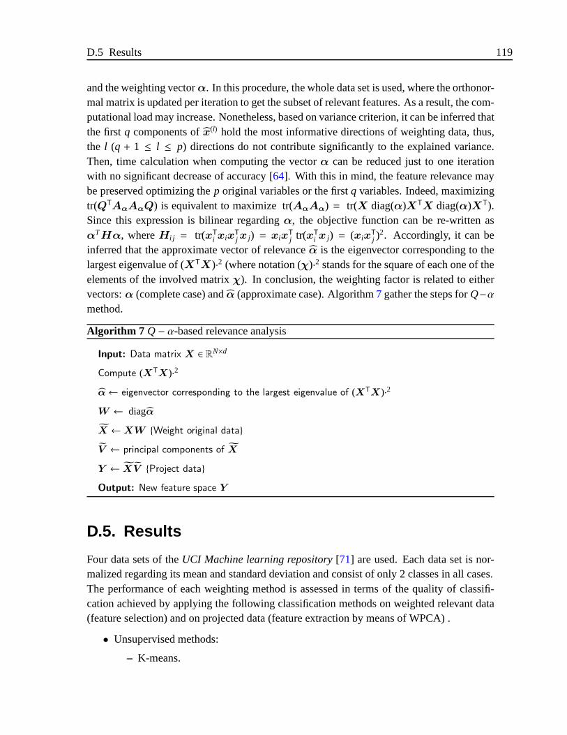
D.5 Results 119
and the weighting vectorα. In this procedure, the whole data set is used, where the orthonor-mal matrix is updated per iteration to get the subset of relevant features. As a result, the com-putational load may increase. Nonetheless, based on variance criterion, it can be inferred thatthe firstq components ofx(l) hold the most informative directions of weighting data, thus,the l (q + 1 ≤ l ≤ p) directions do not contribute significantly to the explained variance.Then, time calculation when computing the vectorα can be reduced just to one iterationwith no significant decrease of accuracy [64]. With this in mind, the feature relevance maybepreserved optimizing thep original variables or the firstq variables. Indeed, maximizingtr(QTAαAαQ) is equivalent to maximize tr(AαAα) = tr(X diag(α)XTX diag(α)XT).Since this expression is bilinear regardingα, the objective function can be re-written asαTHα, whereHi j = tr(xT
i xixTj x j) = xix
Tj tr(xT
i x j) = (xixTj )
2. Accordingly, it can beinferred that the approximate vector of relevanceα is the eigenvector corresponding to thelargest eigenvalue of (XTX)·2 (where notation (χ)·2 stands for the square of each one of theelements of the involved matrixχ). In conclusion, the weighting factor is related to eithervectors:α (complete case) andα (approximate case). Algorithm7 gather the steps forQ−αmethod.
Algorithm 7 Q− α-based relevance analysis
Input: Data matrix X ∈ RN×d
Compute (XTX)·2
α← eigenvector corresponding to the largest eigenvalue of (XTX)·2
W ← diagα
X ←XW Weight original data
V ← principal components of X
Y ← XV Project data
Output: New feature space Y
D.5. Results
Four data sets of theUCI Machine learning repository[71] are used. Each data set is nor-malized regarding its mean and standard deviation and consist of only 2 classes in all cases.The performance of each weighting method is assessed in terms of the quality of classifi-cation achieved by applying the following classification methods on weighted relevant data(feature selection) and on projected data (feature extraction by means of WPCA) .
• Unsupervised methods:
– K-means.
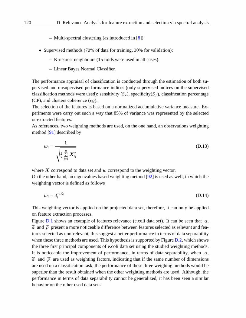
120 D Relevance Analysis for feature extraction and selectionvia spectral analysis
– Multi-spectral clustering (as introduced in [8]).
• Supervised methods (70% of data for training, 30% for validation):
– K-nearest neighbours (15 folds were used in all cases).
– Linear Bayes Normal Classifier.
The performance appraisal of classification is conducted through the estimation of both su-pervised and unsupervised performance indices (only supervised indices on the supervisedclassification methods were used): sensitivity (Se), specificity(Sp), classification percentage(CP), and clusters coherence (ǫM).The selection of the features is based on a normalized accumulative variance measure. Ex-periments were carry out such a way that 85% of variance was represented by the selectedor extracted features.As references, two weighting methods are used, on the one hand, an observations weightingmethod [91] described by
wi =1√
1q
q∑j=1
X2i j
(D.13)
whereX correspond to data set andw correspond to the weighting vector.On the other hand, an eigenvalues based weighting method [92] is used as well, in which theweighting vector is defined as follows
wi = λ−1/2i (D.14)
This weighting vector is applied on the projected data set, therefore, it can only be appliedon feature extraction processes.
FigureD.1 shows an example of features relevance (e.coli data set). It can be seen thatα,α and ρ present a more noticeable difference between features selected as relevant and fea-tures selected as non-relevant, this suggest a better performance in terms of data separabilitywhen these three methods are used. This hypothesis is supported by FigureD.2, which showsthe three first principal components of e.coli data set using the studied weighting methods.It is noticeable the improvement of performance, in terms of data separability, whenα,α and ρ are used as weighting factors, indicating that if the same number of dimensionsare used on a classification task, the performance of these three weighing methods would besuperior than the result obtained when the other weighting methods are used. Although, theperformance in terms of data separability cannot be generalized, it has been seen a similarbehavior on the other used data sets.
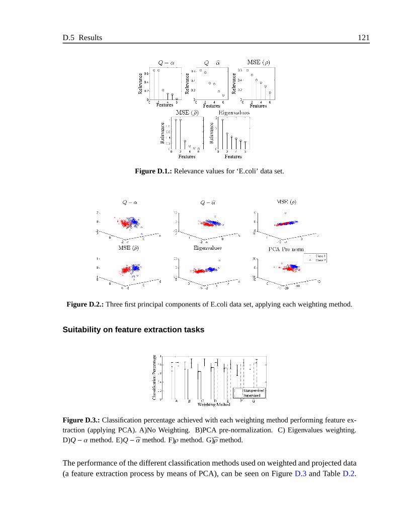
D.5 Results 121
Figure D.1.: Relevance values for ‘E.coli’ data set.
Figure D.2.: Three first principal components of E.coli data set, applying each weighting method.
Suitability on feature extraction tasks
Figure D.3.: Classification percentage achieved with each weighting method performing feature ex-traction (applying PCA). A)No Weighting. B)PCA pre-normalization. C) Eigenvalues weighting.D)Q− α method. E)Q− α method. F)ρ method. G)ρ method.
The performance of the different classification methods used on weighted and projected data(a feature extraction process by means of PCA), can be seen on FigureD.3 and TableD.2.
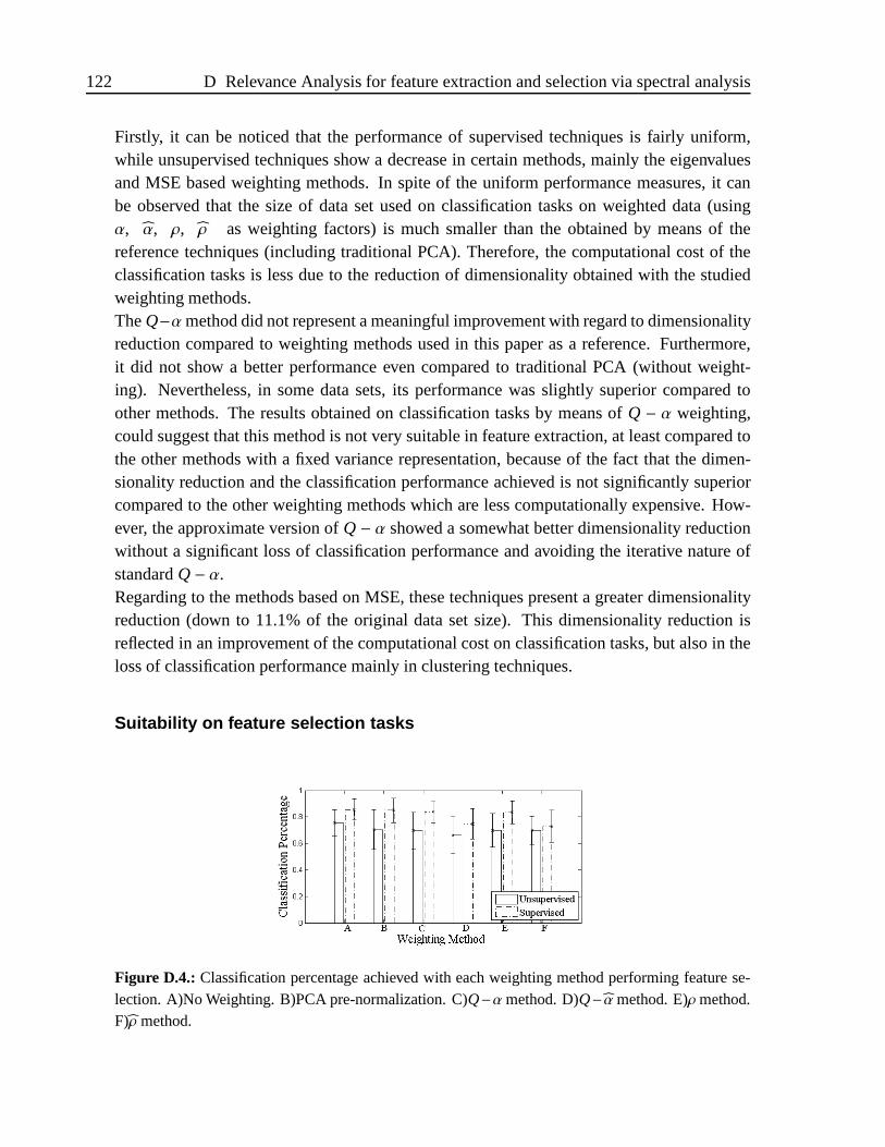
122 D Relevance Analysis for feature extraction and selectionvia spectral analysis
Firstly, it can be noticed that the performance of supervised techniques is fairly uniform,while unsupervised techniques show a decrease in certain methods, mainly the eigenvaluesand MSE based weighting methods. In spite of the uniform performance measures, it canbe observed that the size of data set used on classification tasks on weighted data (usingα, α, ρ, ρ as weighting factors) is much smaller than the obtained by means of thereference techniques (including traditional PCA). Therefore, the computational cost of theclassification tasks is less due to the reduction of dimensionality obtained with the studiedweighting methods.TheQ−αmethod did not represent a meaningful improvement with regard to dimensionalityreduction compared to weighting methods used in this paper as a reference. Furthermore,it did not show a better performance even compared to traditional PCA (without weight-ing). Nevertheless, in some data sets, its performance was slightly superior compared toother methods. The results obtained on classification tasks by means ofQ − α weighting,could suggest that this method is not very suitable in feature extraction, at least compared tothe other methods with a fixed variance representation, because of the fact that the dimen-sionality reduction and the classification performance achieved is not significantly superiorcompared to the other weighting methods which are less computationally expensive. How-ever, the approximate version ofQ− α showed a somewhat better dimensionality reductionwithout a significant loss of classification performance and avoiding the iterative nature ofstandardQ− α.Regarding to the methods based on MSE, these techniques present a greater dimensionalityreduction (down to 11.1% of the original data set size). This dimensionality reduction isreflected in an improvement of the computational cost on classification tasks, but also in theloss of classification performance mainly in clustering techniques.
Suitability on feature selection tasks
Figure D.4.: Classification percentage achieved with each weighting method performing feature se-lection. A)No Weighting. B)PCA pre-normalization. C)Q−αmethod. D)Q− αmethod. E)ρmethod.F)ρ method.
D.5 Results 123
The performance of the different classification methods used on weighted data (this meanswithout applying PCA ) can be seen on FigureD.4 and TableD.3. Using the weightingfactors as a criterion for selecting the most relevant features, it was found that the greater di-mensionality reduction was achieved by means ofQ− α. Additionally, this method presentsa very low computational cost at the expense of loss classification performance (comparedto the other weighting techniques), mostly on supervised classification processes.Regardingρ, it is the best weighting method in terms of computational cost but also is theweighting factor that causes the greatest loss of classification percentage (mainly on super-vised classification tasks) among the used techniques.On the other hand,α and ρ are the factors whose performance (in terms of dimensional-ity reduction) is not very good but its performance in terms of classification percentage isevidently superior, mainly on supervised classification techniques. Furthermore, the classifi-cation performance of the weighting factorρ is slightly inferior than the obtained by meansof α, however, the computational cost of the weighting factorρ is much smaller than theiterativeα.
The best data separability results were obtained by means ofα, α and ρ as weightingfactors. This behavior is explained by the differences between relevant and non relevant fea-tures, which are much more noticeable in these factors, in comparison to the other methodsstudied, where such difference is more uniform between all features. The latter causes arelatively bad data separability.α vector (obtained by means of a non iterative method)showed a great performance, with a much smaller computing time in comparison to standardQ− α but at the same time, keeping almost intact the attributes that cause a remarkable dataseparability. From the point of view of the classifiers performance, it can be seen that whena feature selection task was carried out,ρ and α were the weighting factors that indicated abetter performance in terms of dimensionality reduction and classification quality, although,it is noteworthy thatα classification performance was not bad and additionally achieved aremarkable dimensionality reduction (being 17% of the original data size the average reduc-tion among the tested data sets). Furthermore, when a feature extraction task was carried out,the studied methods showed an homogeneous classification performance, nevertheless,ρ
presented the greatest dimensionality reduction in comparison to the other studied methods.As future work, other weighting factors based on a distance measure should be studied. Ad-ditionally, multi-class data sets with a more complex nature (especially, a more complexseparability) will be used.
Other results
Following are presented another experimental results in tablesD.2 andD.3.

124 D Relevance Analysis for feature extraction and selectionvia spectral analysis
Table D.2.: Classification performance applying feature extraction. Time correspond to the timeneeded to calculate the weighting vector, R% is the dimensionality reduction being 100% the originaldata set
Breast Diabetes Heart Ionosphere Breast Diabetes Heart Ionospherek-means Spectral k-means Spectral k-means Spectral k-means Spectral KNN LCD KNN LCD KNN LCD KNN LCD
Without WeightingCP 0.96 0.701 0.706 0.646 0.832 0.76 0.706 0.741 0.96732 0.961 0.732 0.760 0.821 0.831 0.884 0.883Sp 0.957 0.746 0.562 0.444 0.885 0.694 0.572 0.594 0.974 0.936 0.45 6 0.567 0.74 0.784 0.719 0.721Se 0.962 0.696 0.82 0.656 0.799 0.85 0.818 0.909 0.96391 0.97494 0.88178 0.86356 0.89028 0.87083 0.97512 0.97214ǫM 0.9741 0.7465 0.8333 0.9518 0.758 0.757 0.8916 0.9206 – – – – – – – –
Time –R % 58.4625± 15.8283
PCA pre-normCP 0.957 0.636 0.648 0.649 0.825 0.778 0.692 0.396 0.97026 0.95098 0.71942 0.69333 0.82547 0.8367 0.9 0.769Sp 0.941 0.378 0 0.474 0.89 0.729 0.553 0.052 0.97559 0.90798 0.48167 0.19167 0.73496 0.79837 0.827 0.466Se 0.966 0.652 0.65 0.654 0.787 0.83 0.823 0.525 0.96742 0.97393 0.84622 0.96089 0.90278 0.86944 0.9403 0.936ǫM 0.9807 0.9394 0.919 0.818 0.7533 0.7476 0.8902 0.911 – – – – – – – –
Time 0.0649± 0.0038R % –
EigenvaluesCP 0.965 0.386 0.667 0.646 0.529 0.727 0.746 0.4814 0.95229 0.96111 0.73652 0.75652 0.79176 0.83446 0.902 0.865Sp 0.961 0.216 0.523 0.447 0.465 0.7 100 0 0.93427 0.93052 0.4575 0.56917 0.64065 0.77724 0.753 0.679Se 0.967 0.533 0.738 0.656 0.539 0.752 0.717 0.573 0.9619 0.97744 0.88533 0.85644 0.92083 0.88333 0.985 0.968ǫM 0.9123 0.9775 0.82 0.933 0.7253 0.6892 0.707 0.916 – – – – – – – –
Time 0.0638± 0.0143R % 58.5200±15.8797
Q− αCP 0.953 0.689 0.664 0.643 0.794 0.731 0.712 0.723 0.97157 0.96536 0.7487 0.77971 0.82547 0.83895 0.858 0.840Sp 0.955 0.642 0.519 0.421 0.811 0.652 0.724 0.586 0.97559 0.93427 0.51 0.60083 0.75122 0.80163 0.666 0.632Se 0.952 0.697 0.735 0.655 0.783 0.864 0.852 0.852 0.96942 0.98195 0.876 0.87511 0.88889 0.87083 0.965 0.955ǫM 0.9665 0.9849 0.891 0.938 0.8447 0.8979 0.9541 0.9575 – – – – – – – –
Time 1.6375±0.9358R % 51.6375±17.6951
Q− αCP 0.957 0.684 0.672 0.640 0.737 0.673 0.712 0.721 0.96699 0.95948 0.68957 0.67855 0.76779 0.79176 0.829 0.815Sp 0.964 0.725 0.531 0.488 0.7 0.607 0.577 0.583 0.9615 0.91174 0.35333 0.32417 0.64715 0.68455 0.6108 0.594Se 0.954 0.68 0.743 0.7511 0.773 0.784 0.826 0.847 0.96992 0.98496 0.86889 0.86756 0.87083 0.88333 0.950 0.937ǫM 0.9719 0.9791 0.9405 0.943 0.833 0.853 0.946 0.949 – – – – – – – –
Time 0.0761±0.0048R % 48.0750±10.5792
MSEρCP 0.915 0.594 0.671 0.645 0.656 0.656 0.749 0.493 0.962 0.95327 0.75101 0.7713 0.78951 0.82097 .881 0.8602Sp 0.95 0.372 0.528 0.444 0.597 0.595 100 0 0.95023 0.90141 0.46667 0.57417 0.73496 0.7626 0.731 0.661Se 0.9 0.656 0.747 0.655 0.746 0.759 0.7188 0.579 0.96792 0.98095 0.90267 0.87644 0.83611 0.87083 0.964 0.9701ǫM 0.9915 0.8126 0.8949 0.9725 0.8042 0.8102 0.9825 0.9631 – – – – – – – –
Time 0.0837±0.0037R % 42.62±22.4201
MSE ρCP 0.91 0.65 0.605 0.583 0.694 0.69 0.709 0.709 0.96699 0.95784 0.74261 0.77942 0.82172 0.81873 0.855 0.815Sp 0.978 0 0.448 0.387 0.644 0.642 0.579 0.571 0.95775 0.91362 0.47167 0.55917 0.73496 0.76585 0.691 0.616Se 0.885 0.65 0.731 0.6672 0.752 0.746 0.809 0.84 0.97193 0.98145 0.88711 0.89689 0.89583 0.86389 0.945 0.925ǫM 0.9995 0.8402 0.9536 0.9928 0.9983 0.9983 0.9604 0.9647 – – – – – – – –
Time 0.06± 0.0037R % 22.465±11.1647
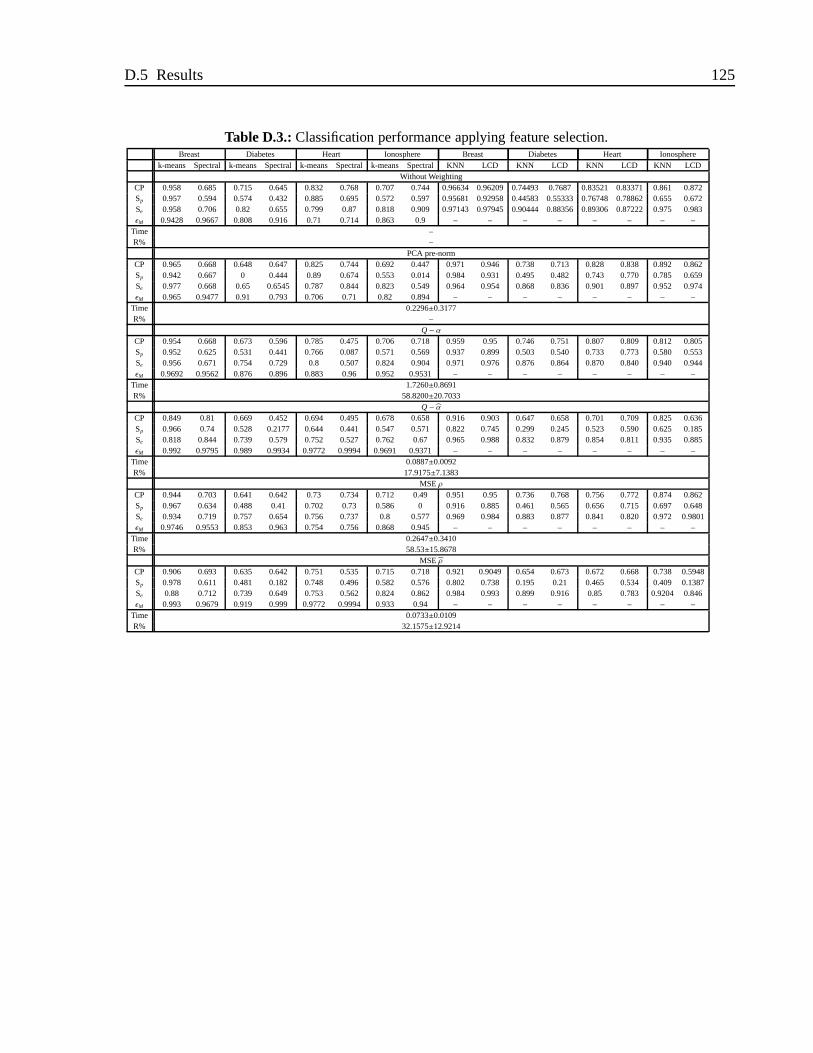
D.5 Results 125
Table D.3.:Classification performance applying feature selection.Breast Diabetes Heart Ionosphere Breast Diabetes Heart Ionosphere
k-means Spectral k-means Spectral k-means Spectral k-means Spectral KNN LCD KNN LCD KNN LCD KNN LCDWithout Weighting
CP 0.958 0.685 0.715 0.645 0.832 0.768 0.707 0.744 0.96634 0.96209 0.74493 0.7687 0.83521 0.83371 0.861 0.872Sp 0.957 0.594 0.574 0.432 0.885 0.695 0.572 0.597 0.95681 0.92958 0.44583 0.55333 0.76748 0.78862 0.655 0.672Se 0.958 0.706 0.82 0.655 0.799 0.87 0.818 0.909 0.97143 0.97945 0.90444 0.88356 0.89306 0.87222 0.975 0.983ǫM 0.9428 0.9667 0.808 0.916 0.71 0.714 0.863 0.9 – – – – – – – –
Time –R% –
PCA pre-normCP 0.965 0.668 0.648 0.647 0.825 0.744 0.692 0.447 0.971 0.946 0.738 0.713 0.828 0.838 0.892 0.862Sp 0.942 0.667 0 0.444 0.89 0.674 0.553 0.014 0.984 0.931 0.495 0.482 0.743 0.770 0.785 0.659Se 0.977 0.668 0.65 0.6545 0.787 0.844 0.823 0.549 0.964 0.954 0.868 0.836 0.901 0.897 0.952 0.974ǫM 0.965 0.9477 0.91 0.793 0.706 0.71 0.82 0.894 – – – – – – – –
Time 0.2296±0.3177R% –
Q− αCP 0.954 0.668 0.673 0.596 0.785 0.475 0.706 0.718 0.959 0.95 0.746 0.751 0.807 0.809 0.812 0.805Sp 0.952 0.625 0.531 0.441 0.766 0.087 0.571 0.569 0.937 0.899 0.503 0.540 0.733 0.773 0.580 0.553Se 0.956 0.671 0.754 0.729 0.8 0.507 0.824 0.904 0.971 0.976 0.876 0.864 0.870 0.840 0.940 0.944ǫM 0.9692 0.9562 0.876 0.896 0.883 0.96 0.952 0.9531 – – – – – – – –
Time 1.7260±0.8691R% 58.8200±20.7033
Q− αCP 0.849 0.81 0.669 0.452 0.694 0.495 0.678 0.658 0.916 0.903 0.647 0.658 0.701 0.709 0.825 0.636Sp 0.966 0.74 0.528 0.2177 0.644 0.441 0.547 0.571 0.822 0.745 0.299 0.245 0.523 0.590 0.625 0.185Se 0.818 0.844 0.739 0.579 0.752 0.527 0.762 0.67 0.965 0.988 0.832 0.879 0.854 0.811 0.935 0.885ǫM 0.992 0.9795 0.989 0.9934 0.9772 0.9994 0.9691 0.9371 – – – – – – – –
Time 0.0887±0.0092R% 17.9175±7.1383
MSEρCP 0.944 0.703 0.641 0.642 0.73 0.734 0.712 0.49 0.951 0.95 0.736 0.768 0.756 0.772 0.874 0.862Sp 0.967 0.634 0.488 0.41 0.702 0.73 0.586 0 0.916 0.885 0.461 0.565 0.656 0.715 0.697 0.648Se 0.934 0.719 0.757 0.654 0.756 0.737 0.8 0.577 0.969 0.984 0.883 0.877 0.841 0.820 0.972 0.9801ǫM 0.9746 0.9553 0.853 0.963 0.754 0.756 0.868 0.945 – – – – – – – –
Time 0.2647±0.3410R% 58.53±15.8678
MSE ρCP 0.906 0.693 0.635 0.642 0.751 0.535 0.715 0.718 0.921 0.9049 0.654 0.673 0.672 0.668 0.738 0.5948Sp 0.978 0.611 0.481 0.182 0.748 0.496 0.582 0.576 0.802 0.738 0.195 0.21 0.465 0.534 0.409 0.1387Se 0.88 0.712 0.739 0.649 0.753 0.562 0.824 0.862 0.984 0.993 0.899 0.916 0.85 0.783 0.9204 0.846ǫM 0.993 0.9679 0.919 0.999 0.9772 0.9994 0.933 0.94 – – – – – – – –
Time 0.0733±0.0109R% 32.1575±12.9214

E. Academic discussion
Conference papers
2013:
[1]. D. H. Peluffo-Ordonez, A. E. Castro-Ospina, D. Chavez-Chamorro, C. D. Acosta-Medina, and G. Castellanos-Domınguez.“Normalized Cuts Clustering withPrior Knowledge and a Pre-clustering Stage”. In: European Symposium onArtificial Neural Networks, Computational Intelligence and Machine Learning -ESANN 2013. Belgium.
[2]. D. H. Peluffo-Ordonez, S. Garcıa-Vega, G. Castellanos-Domınguez.“KernelSpectral Clustering for Motion Tracking: A first approach”. In: InternationalWork-Conference on the Interplay between Natural and Artificial Computation -IWINAC 2013. Spain.
[3]. D. H. Peluffo-Ordonez, S. Garcıa-Vega, R. Langone, J. A. K. Suykens, G. Castellanos-Domınguez.“Kernel Spectral Clustering for dynamic data using Multiple Ker-nel Learning”. In: International Joint Conference on Neural Networks - IJCNN2013. EEUU.Submitted.
[4]. D. H. Peluffo-Ordonez, S. Garcıa-Vega, G. Castellanos-Domınguez.“KernelSpectral Clustering for dynamic data”. In: International Conference on Com-puter Vision - ICCV 2013. Australia.To be submitted.
[5]. A. E. Castro-Ospina, C. Castro-Hoyos, D. H. Peluffo-Ordonez, G. Daza-Santacoloma,G. Castellanos-Domınguez.“Novel Heuristic Search for Ventricular Arrhyth-mia Detection using Normalized Cut Clustering”. In: The 35th Annual Interna-tional Conference of the IEEE Engineering in Medicine and Biology Society -EMBC’13. Osaka, Japan.Submitted.
2012:
[1]. D. H. Peluffo, C. D. Acosta, G. Castellanos.“An improved multi-class clusteringbased on normalized cuts”. In: Ibero-American Congress on Pattern Recognition- CIARP 2012. Argentina.
[2]. S. Molina-Giraldo, A. M. Alvarez-Meza, D. H. Peluffo-Ordonez and G. Castel-lanos Dominguez.“Image Segmentation based on Multiple Kernel Representa-

127
tion” . In: Ibero-American Conference on Artificial Intelligence - IBERAMIA2012.
[3]. J. L. Rodrıguez, D. H. Peluffo-Ordonez, D. Cuesta and G. Castellanos.“Gen-eralized distance measure based WPCA for unsupervised analysis of ECG sig-nals”. In: Computers in Cardiology - CINC 2012. Poland.
[4]. C. Castro, D. H. Peluffo-Ordonez and C. G. Castellanos.“Constrained affinitymatrix for spectral clustering: A basic semi-supervised extension”. In: Sympo-sium of Image, Signal Processing, and Artificial Vision - STSIVA 2012. Colom-bia.
[5]. L. M. Morales-Villamil, M. C. Garcıa-Murillo, D. H. Peluffo-Ordonez and C.G. Castellanos-Domınguez.“Relevance Analysis based on graph theory andspectral analysis”. In: Symposium of Image, Signal Processing, and ArtificialVision - STSIVA 2012. Colombia.
2011:
[1]. E. Giraldo, D. H. Peluffo-Ordonez, G. Castellanos-Domınguez.“Weighted TimeSeries Analysis for Electroencephalographic Source Localization”. In: VII In-ternational Seminar on Medical Information Processing and Analysis - SIPAIM2011. Colombia.
[2]. C. Castro, A. E. Castro, D. H. Peluffo, G. Castellanos.“On the groups numberestimation for unsupervised clustering”. In: XVI Symposium of Image, SignalProcessing, and Artificial Vision - STSIVA 2011. Colombia.
[3]. J.S. Castano-Candamil, S. Garcıa-Vega, D. H. Peluffo-Ordonez, C.G. Castellanos-Domınguez.“A Comparative Study of Weighting Factors for WPCA Based on aGeneralized Distance Measure”. In: XVI Symposium of Image, Signal Process-ing, and Artificial Vision - STSIVA 2011. Colombia.
2010:
[1]. D. H. Peluffo-Ordonez, D. F. Lopez, J. L. Rodrıguez and G. Castellanos.“Affinitymatrix selection for spectral clustering”. In: XV Symposium of Image, SignalProcessing, and Artificial Vision (STSIVA). STSIVA, 2010. Bogota, Colombia.
[2]. J. L. Rodrıguez, E. Delgado, D. H. Peluffo-Ordonez, D. Cuesta and G. Castel-lanos.“Weighted-PCA for Unsupervised Analysis of Cardiac Arrhythmias”. In:Engineering in Medicine and Biology Conference. EMBC, 2010. Argentina.

128 E Academic discussion
Journals
2012:
[1]. D. H. Peluffo-Ordonez, C. Alzate, J. A. K. Suykens and G. Castellanos.OptimalData Projection. In: Pattern Recognition Letters.Submitted.
[2]. J.L. Rodrıguez-Sotelo, D. H. Peluffo-Ordonez, D. Cuesta-Frau and G. Castellanos-Domınguez.Unsupervised feature relevance analysis applied to improve ECGheartbeat clustering. In: Computer Methods and Programs in Biomedicine.
[3]. E. Giraldo, D. H. Peluffo-Ordonez and G. Castellanos-DomınguezWeighted timeseries analysis for electroencephalographic source localization. In: DYNA -Medellın, Colombia.
Book chapters
2012:
[1]. D. H. Peluffo-Ordonez, D. Cuesta-Frau and G. Castellanos-Domınguez.Unsu-pervised classification of arrhythmias for Holter recordings. In: Electrocardio-grams (ISBN 980-953-307-828-6).Submitted.

Bibliography
[1] A. Agarwal and B. Triggs. Monocular human motion capture with a mixture of regres-sors. InComputer Vision and Pattern Recognition-Workshops, 2005. CVPR Workshops.IEEE Computer Society Conference on, pages 72–72. IEEE, 2005.
[2] D.N. Truong Cong, L. Khoudour, C. Achard, C. Meurie, and O. Lezoray. People re-identification by spectral classification of silhouettes.Signal Processing, 90(8):2362–2374, 2010.
[3] L. You, S. Zhou, G. Gao, and M. Leng. Scalable spectral clustering combined withadjacencies merging for image segmentation.Advances in Computer, Communication,Control and Automation, pages 709–717, 2012.
[4] L. Wang and M. Dong. Multi-level low-rank approximation-based spectral clusteringfor image segmentation.Pattern Recognition Letters, 2012.
[5] S. Molina-Giraldo, A. Alvarez-Meza, D. Peluffo-Ordonez, and G. Castellanos-Domınguez. Image segmentation based on multi-kernel learning and feature relevanceanalysis.Advances in Artificial Intelligence–IBERAMIA 2012, pages 501–510, 2012.
[6] A. Ekin, S. Pankanti, and A. Hampapur. Initialization-independent spectral cluster-ing with applications to automatic video analysis. InAcoustics, Speech, and SignalProcessing, 2004. Proceedings.(ICASSP’04). IEEE International Conference on, vol-ume 3, pages iii–641. IEEE, 2004.
[7] D.Q. Zhang, C.Y. Lin, S.F. Chang, and J.R. Smith. Semantic video clustering acrosssources using bipartite spectral clustering. InMultimedia and Expo, 2004. ICME’04.2004 IEEE International Conference on, volume 1, pages 117–120. IEEE, 2004.
[8] Yu Stella X. and Shi Jianbo. Multiclass spectral clustering. InICCV ’03: Proceedingsof the Ninth IEEE International Conference on Computer Vision, page 313, Washing-ton, DC, USA, 2003. IEEE Computer Society.
[9] P. K. Chan, M. D. F. Schlag, and J. T. Zien. Spectral K-way ratio cut partitioning andclustering. IEEE Transactions on Computer-aided Design of Integrated Circuits andSystems, 13:1088 – 1096, 1994.

130 Bibliography
[10] Jianbo Shi and J. Malik. Normalized cuts and image segmentation. Pattern Analysisand Machine Intelligence, IEEE Transactions on, 22(8):888–905, Aug 2000.
[11] F.R.K. Chung.Spectral graph theory. Amer Mathematical Society, 1997.
[12] Andrew Y. Ng, Michael I. Jordan, and Yair Weiss. On spectral clustering: Analysisand an algorithm. InAdvances in Neural Information Processing Systems 14, pages849–856. MIT Press, 2001.
[13] L. Hagen and A.B. Kahng. New spectral methods for ratio cut partitioning and clus-tering.Computer-Aided Design of Integrated Circuits and Systems, IEEE Transactionson, 11(9):1074–1085, 1992.
[14] J. Shi and J. Malik. A random walks view of spectral segmentation.In AI and Statistics(AISTATS, 2001.
[15] D. Peluffo, C. D. Acosta, and G. Castellanos. An improved multi-class spectral clus-tering based on normalized cuts.XVII Iberoamerican Congress on Pattern Recognition- CIARP, 2012.
[16] C. Alzate and J.A.K. Suykens. Multiway spectral clustering with out-of-sample ex-tensions through weighted kernel PCA.IEEE transactions on pattern analysis andmachine intelligence, pages 335–347, 2008.
[17] F.R. Bach and M.I. Jordan. Learning spectral clustering, with application to speechseparation.The Journal of Machine Learning Research, 7:1963–2001, 2006.
[18] Lihi Zelnik-manor and Pietro Perona. Self-tuning spectral clustering. InAdvances inNeural Information Processing Systems 17, pages 1601–1608. MIT Press, 2004.
[19] C. Ding and X. He. Linearized cluster assignment via spectral ordering. InMA-CHINE LEARNING-INTERNATIONAL WORKSHOP THEN CONFERENCE-, vol-ume 21, page 233. Citeseer, 2004.
[20] J. Ham, D.D. Lee, S. Mika, and B. Scholkopf. A kernel view of the dimensionalityreduction of manifolds. InProceedings of the twenty-first international conference onMachine learning, page 47. ACM, 2004.
[21] C. Alzate and J.A.K. Suykens. A weighted kernel PCA formulation with out-of-sampleextensions for spectral clustering methods. InNeural Networks, 2006. IJCNN’06. In-ternational Joint Conference on, pages 138–144. IEEE, 2006.
[22] B. Takacs, S. Butler, and Y. Demiris. Multi-agent behaviour segmentation via spectralclustering. InProceedings of the AAAI-2007, PAIR Workshop, pages 74–81.
Bibliography 131
[23] F. Zhou, F. Torre, and J.K. Hodgins. Aligned cluster analysis for temporal segmentationof human motion. InAutomatic Face & Gesture Recognition, 2008. FG’08. 8th IEEEInternational Conference on, pages 1–7. IEEE, 2008.
[24] A.B. Chan and N. Vasconcelos. Probabilistic kernels for the classification of auto-regressive visual processes. 2005.
[25] J. Keshet and S. Bengio.Automatic speech and speaker recognition: Large margin andkernel methods. Wiley, 2009.
[26] M.L. Maestri, M.C. Cassanello, and G.I. Horowitz. Kernel pca performance in pro-cesses with multiple operation modes.Chemical Product and Process Modeling,4(5):7, 2009.
[27] S.W. Choi and I.B. Lee. Nonlinear dynamic process monitoring based on dynamickernel pca.Chemical engineering science, 59(24):5897–5908, 2004.
[28] Bruce Hendrickson and Robert Leland. An improved spectral graph partitioning al-gorithm for mapping parallel computations.SIAM Journal on Scientific Computing,16(2):452–469, 1995.
[29] Bui The Anh and D. D. X. Thanh. A perron-frobenius theorem for positive quasipoly-nomial matrices associated with homogeneous difference equations.Journal of appliedmathematics, 2007.
[30] Andrew Y. Ng, Michael I. Jordan, and Yair Weiss. On spectral clustering: Analysisand an algorithm. InAdvances in Neural Information Processing Systems 14, pages849–856. MIT Press, 2001.
[31] Greg Hamerly and Charles Elkan. Alternatives to the k-means algorithm that find betterclusterings. InCIKM ’02: Proceedings of the eleventh international conference onInformation and knowledge management, pages 600–607, New York, NY, USA, 2002.ACM.
[32] Inderjit S. Dhillon, Yuqiang Guan, and Brian Kulis. Kernel k-means, spectral clusteringand normalized cuts. 2004.
[33] Desmond Higham and Milla Kibble. A unified view of spectral clustering. InMathe-matics Research Report 2, University of Strathclyde, 2004.
[34] Y. Bengio, J.F. Paiement, P. Vincent, O. Delalleau, N. Le Roux, and M. Ouimet. Out-of-sample extensions for lle, isomap, mds, eigenmaps, and spectral clustering. InAd-vances in neural information processing systems 16: proceedings of the 2003 confer-ence, volume 16, page 177. The MIT Press, 2004.

132 Bibliography
[35] C. Fowlkes, S. Belongie, F. Chung, and J. Malik. Spectral grouping using the Nystrommethod.IEEE Transactions on Pattern Analysis and Machine Intelligence, pages 214–225, 2004.
[36] C.T.H. Baker. The numerical treatment of integral equations, volume 13. Clarendonpress Oxford, UK, 1977.
[37] C. Williams and M. Seeger. Using the Nystrom method to speed up kernel machines.In Advances in Neural Information Processing Systems 13. Citeseer, 2001.
[38] B. Scholkopf, A. Smola, and K.R. Muller. Nonlinear component analysis as a kerneleigenvalue problem.Neural computation, 10(5):1299–1319, 1998.
[39] J.A.K. Suykens, T. Van Gestel, J. De Brabanter, B. De Moor, and J. Vandewalle.Leastsquares support vector machines. World Scientific Pub Co Inc, 2002.
[40] JAK Suykens, T. Van Gestel, J. Vandewalle, and B. De Moor. A support vector machineformulation to PCA analysis and its kernel version.Neural Networks, IEEE Transac-tions on, 14(2):447–450, 2003.
[41] C. Alzate and J. Suykens. Sparse kernel models for spectral clustering using the in-complete cholesky decomposition. InNeural Networks, 2008. IJCNN 2008.(IEEEWorld Congress on Computational Intelligence). IEEE International Joint Conferenceon, pages 3556–3563. IEEE, 2008.
[42] Sareh Shirazi, Mehrtash T Harandi, Conrad Sanderson, Azadeh Alavi, and Brian CLovell. Clustering on grassmann manifolds via kernel embedding with application toaction analysis. InProc. IEEE International Conference on Image Processing, 2012.
[43] LR Sudha and R Bhavani. Performance comparison of svm and knn in automaticclassification of human gait patterns.Int. J. Comput, 6(1):19–28, 2012.
[44] Rocco Langone, Carlos Alzate, and Johan AK Suykens. Kernel spectral clustering withmemory effect.Physica A: Statistical Mechanics and its Applications, 2013.
[45] F. Gonzalez, D. Bermeo, L. Ramos, and O. Nasraoui. On the robustness of kernel-based clustering.Progress in Pattern Recognition, Image Analysis, Computer Vision,and Applications, pages 122–129, 2012.
[46] H.C. Huang, Y.Y. Chuang, and C.S. Chen. Multiple kernel fuzzy clustering.FuzzySystems, IEEE Transactions on, 20(1):120–134, 2012.
[47] I.S. Dhillon, Y. Guan, and B. Kulis. Weighted graph cuts without eigenvectors a mul-tilevel approach.Pattern Analysis and Machine Intelligence, IEEE Transactions on,29(11):1944–1957, 2007.

Bibliography 133
[48] L. Xu, W. Li, and D. Schuurmans. Fast normalized cut with linear constraints. InComputer Vision and Pattern Recognition, 2009. CVPR 2009. IEEE Conference on,pages 2866–2873. IEEE, 2009.
[49] Pak K. Chan, Martine Schlag, and Jason Y. Zien. Spectral k-way ratio-cut partition-ing and clustering. InProceedings of the 1993 symposium on Research on integratedsystems, pages 123–142, Cambridge, MA, USA, 1993. MIT Press.
[50] Marina Maila and Jianbo Shi. Learning segmentation by random walk. InNeuralInformation Processing Systems (NIPS), 2001.
[51] I.S. Dhillon, Y. Guan, and B. Kulis. Kernel k-means: spectral clustering and nor-malized cuts. InProceedings of the tenth ACM SIGKDD international conference onKnowledge discovery and data mining, pages 551–556. ACM, 2004.
[52] D.S. Cvetkovic-Ilic. Re-nnd solutions of the matrix equation axb= c.Journal of theAustralian Mathematical Society, 84(1):63–72, 2008.
[53] A. Ben-Israel and T.N.E. Greville.Generalized inverses: theory and applications,volume 15. Springer Verlag, 2003.
[54] M. Filippone, F. Camastra, F. Masulli, and S. Rovetta. A survey of kernel and spectralmethods for clustering.Pattern recognition, 41(1):176–190, 2008.
[55] C. Alzate and J. A. K. Suykens. Multiway spectral clustering with out-of-sample exten-sions through weighted kernel pca.Pattern Analysis and Machine Intelligence, IEEETransactions on, 32(2):335–347, 2010.
[56] Sangkeun Lee and M.H. Hayes. Properties of the singular value decomposition forefficient data clustering.Signal Processing Letters, IEEE, 11(11):862–866, Nov. 2004.
[57] L. Wolf and S. Bileschi. Combining variable selection with dimensionality reduction.In Computer Vision and Pattern Recognition, 2005. CVPR 2005. IEEE Computer Soci-ety Conference on, volume 2, pages 801 – 806 vol. 2, june 2005.
[58] Lior Wolf and Amnon Shashua. Feature selection for unsupervised and supervisedinference: The emergence of sparsity in a weight-based approach.Journal of machinelearning, 6:1855 – 1887, 2005.
[59] M. Seeland, A. Karwath, and S. Kramer. A structural cluster kernel for learning ongraphs. InProceedings of the 18th ACM SIGKDD international conference on Knowl-edge discovery and data mining, pages 516–524. ACM, 2012.

134 Bibliography
[60] D. Satish and C. Sekhar. Kernel based clustering for multiclass data. InNeural Infor-mation Processing, pages 1266–1272. Springer, 2004.
[61] C. Domeniconi, J. Peng, and B. Yan. Composite kernels for semi-supervised clustering.Knowledge and information systems, 28(1):99–116, 2011.
[62] J.E. Ormrod and K.M. Davis.Human learning. Merrill, 2004.
[63] B. Scholkopf and A. J. Smola.Learning with Kernels. 2002.
[64] Lior Wolf and Amnon Shashua. Feature selection for unsupervised and supervisedinference: The emergence of sparsity in a weight-based approach.Journal of machinelearning, 6:1855 – 1887, 2005.
[65] Jose Luis Rodrıguez-Sotelo, David Cuesta-Frau, Diego Hernan Peluffo-Ordonez, andCesar German Castellanos-Domınguez. Unsupervised feature selection in cardiac ar-rhythmias analysis. InEngineering in Medicine and Biology Society, 2009. EMBC2009. Annual International Conference of the IEEE, pages 2571 –2574, 3-6 2009.
[66] L. Wolf and S. Bileschi. Combining variable selection with dimensionality reduction.In Computer Vision and Pattern Recognition, 2005. CVPR 2005. IEEE Computer Soci-ety Conference on, volume 2, pages 801 – 806 vol. 2, june 2005.
[67] J.L. Rodrıguez-Sotelo, E. Delgado-Trejos, D. Peluffo-Ordonez, D. Cuesta-Frau, andG. Castellanos-Domınguez. Weighted-pca for unsupervised classification of cardiacarrhythmias. InEngineering in Medicine and Biology Society (EMBC), 2010 AnnualInternational Conference of the IEEE, pages 1906 –1909, 31 2010-sept. 4 2010.
[68] J.L. Rodrıguez-Sotelo, D. Peluffo-Ordonez, D. Cuesta-Frau, and G. Castellanos-Domınguez. Unsupervised feature relevance analysis applied to improve ecg heartbeatclustering.Computer Methods and Programs in Biomedicine, 2012.
[69] Lior Wolf and Amnon Shashua. Feature selection for unsupervised and supervisedinference: The emergence of sparsity in a weight-based approach.J. Mach. Learn.Res., 6:1855–1887, December 2005.
[70] Cuimei Guo, Sheng Zheng, Yaocheng Xie, and Wei Hao. A survey on spectral cluster-ing. In World Automation Congress (WAC), 2012, pages 53–56. IEEE, 2012.
[71] A. Frank and A. Asuncion. UCI machine learning repository, 2010.
[72] R.P.W. Duin, P. Juszczak, P. Paclık, E. Pekalska, D. de Ridder, D.M.J. Tax, andS. Verzakov. PR-Tools4.1, a matlab toolbox for pattern recognition, 2007.

Bibliography 135
[73] D. Martin, C. Fowlkes, D. Tal, and J. Malik. A database of human segmented naturalimages and its application to evaluating segmentation algorithms and measuring eco-logical statistics. InProc. 8th Int’l Conf. Computer Vision, volume 2, pages 416–423,July 2001.
[74] William M Rand. Objective criteria for the evaluation of clustering methods.Journalof the American Statistical association, 66(336):846–850, 1971.
[75] Lawrence Hubert and Phipps Arabie. Comparing partitions.Journal of classification,2(1):193–218, 1985.
[76] Ka Yee Yeung and Walter L Ruzzo. Details of the adjusted rand index and cluster-ing algorithms, supplement to the paper “an empirical study on principal componentanalysis for clustering gene expression data”.Bioinformatics, 17(9):763–774, 2001.
[77] Thomas M Cover, Joy A Thomas, and John Kieffer. Elements of information theory.SIAM Review, 36(3):509–510, 1994.
[78] Alexander Strehl and Joydeep Ghosh. Cluster ensembles—a knowledge reuse frame-work for combining multiple partitions.The Journal of Machine Learning Research,3:583–617, 2003.
[79] Nguyen Xuan Vinh, Julien Epps, and James Bailey. Information theoretic measures forclusterings comparison: Variants, properties, normalization and correction for chance.The Journal of Machine Learning Research, 11:2837–2854, 2010.
[80] L. Vendramin, R. Campello, and E.R. Hruschka. On the comparison of relative clus-tering validity criteria. InProceedings of the SIAM International Conference on DataMining, SIAM, pages 733–744, 2009.
[81] Tadeusz Calinski and Jerzy Harabasz. A dendrite method for cluster analysis.Commu-nications in Statistics-theory and Methods, 3(1):1–27, 1974.
[82] P. Hansen and N. Mladenovic. J-means: a new local search heuristic for minimum sumof squares clustering.Pattern Recognition, pages 405 – 413, 2001.
[83] A. Strehl and J. Ghosh. Cluster ensembles - a knowledge reuse framework for combin-ing multiple partitions.Journal of Machine Learning Research, 3:583–617, 2002.
[84] L. Hubert and P. Arabie. Comparing partitions.Journal of Classification, 1(2):193–218, 1985.
[85] C. Rosenberger and K. Chehdi. Genetic fusion: application to multi-components im-age segmentation. InAcoustics, Speech, and Signal Processing, 2000. ICASSP’00.
136 Bibliography
Proceedings. 2000 IEEE International Conference on, volume 6, pages 2223–2226.IEEE, 2000.
[86] Ranjith Unnikrishnan, Caroline Pantofaru, and Martial Hebert. Toward objective eval-uation of image segmentation algorithms.Pattern Analysis and Machine Intelligence,IEEE Transactions on, 29(6):929–944, 2007.
[87] H. Zha, C. Ding, M. Gu, X. He, and H. Simon. Spectral relaxation for k-means clus-tering. Advances in neural information processing systems, 14:1057–1064, 2001.
[88] C.E. Rasmussen and C.K.I. Williams.Gaussian processes for machine learning, vol-ume 1. MIT press Cambridge, MA, 2006.
[89] H. Henry Yue and Masayuki Tomoyasu. Weighted principal component analysis andits applications to improve fdc performance. InConference on decision and control,2004.
[90] V. Perlibakas. Distance measures for pca-based face recognition.Pattern RecognitionLetters, 25(16):711–724, April 2004.
[91] Diego Hernan Peluffo-Ordonez, Jose Luis Rodrıguez-Sotelo, David Cuesta-Frau, andCesar German Castellanos-Domınguez. Estudio comparativo de metodos de se-leccion de caracaterısticas de inferencia supervisada y no supervisada.Tecno Logicas,(23):149–166, December 2009.
[92] Hui Y. Wang and Xiao J. Wu. Weighted PCA space and its application in face recogni-tion. In Machine Learning and Cybernetics, 2005. Proceedings of 2005 InternationalConference on, volume 7, 2005.