Dynamic mesh: beyond Fluent - Tor Vergata Kartingtorvergata-karting.it/...mesh_2007_Biancolini.pdf · Dynamic mesh: beyond FluentDynamic mesh: beyond Fluent Marco Evangelos Biancolini

www.torvergata-karting.it

Dynamic mesh: beyond FluentDynamic mesh: beyond Fluent

Marco Evangelos BiancoliniDepartment of Mechanical Engineering

University of Rome “Tor Vergata”

Marco Evangelos BiancoliniDepartment of Mechanical Engineering

University of Rome “Tor Vergata”


OutlineOutline

Why use smoothingReview of methods for mesh smoothingPseudo solid approach, FEM solverRadial basis approachExample 2DExample 3D


Why?Why?

Smoothing means that mesh topology is preserved: no new mesh required!Shape optimisationMoving or deforming boundaries (Fluid structure interaction, rigid body movements, morphing)Parametric analysis


Review of scientific contributionsReview of scientific contributions

198 relevant publications in the last 7 years (keyword “moving mesh method”) scanned25 fully examined Strategies:

Laplacian smoothingSpring models (rotational spring correction)Pseudo solid (variable moduli, fictitious loads correction)Boundary methodsOthers…


Selected papers…Selected papers…

AUTOMATIC MESH MOTION FOR THE UNSTRUCTURED FINITE VOLUME METHOD Hrvoje Jasak,ˇZeljko Tukovi´c ISSN 1333–1124An adaptive mesh rezoning scheme for moving boundary flows and fluid–structure interaction Computers and Fluids Volume: 36, Issue: 1, January, 2007, pp. 77-91 Masud, Arif; Bhanabhagvanwala, Manish; Khurram, Rooh A.A three-dimensional torsional spring analogy method for unstructured dynamic meshes Computers and Structures Volume: 80, Issue: 3-4, February, 2002, pp. 305-316 Degand, Christoph; Farhat, CharbelMesh deformation using radial basis functions for gradient-based aerodynamic shape optimization Computers and Fluids Volume: 36, Issue: 6, July, 2007, pp. 1119-1136 Jakobsson, S.; Amoignon, O.Mesh deformation based on radial basis function interpolationComputers and Structures Volume: 85, Issue: 11-14, June - July, 2007, pp. 784-795 de Boer, A.; van der Schoot, M.S.; Bijl, H.Finite element mesh update methods for fluid–structure interaction simulations Finite Elements in Analysis and Design Volume: 40, Issue: 9-10, June, 2004, pp. 1259-1269 Xu, Zhenlong; Accorsi, Michael


Pseudo solid approachPseudo solid approach

The mesh is supposed to be a deformable structureElastic moduli can be chosen on an element by element basis to minimise distortionCorrective loads are added to improve element quality after mesh deformationOne step method: Masud strategy in which stiffness is proportional to element area (volume)Two step methods: stiffness correction and extra loads added to preserve elements shape


Pseudo solid approachPseudo solid approach

Element distortion estimator: ratio between inner and outer circle radii (for triangles)Advantages

Very good results optimising element stiffnessPhysical pseudo solid guarantees mesh compatibilityLarge motions can be handled by means of non linear FEM modelling

Pitfalls:Large problem solutionLarge memory usage (can be alleviated by means of explicit solver)Non conformal meshes, connectors and polyedra requires special treatment


Implementation details (2D)Implementation details (2D)

Node positions of the original mesh read from a nastran data file (GRID, CTRIA3, PSHELL, MAT1, SPC and SPCD entries are processed)Processing

Stiffness matrix is computed for each elementDOF are numbered and stored in ID and LM matrixesAugmented stiffness matrix is assembledLinear system is solved

CheckingResidual is calculatedComparison with nastran solution

Deformed grid is represented by a scatter plotElement distortion is calculated



Material stiffness matrixElement areaInterpolation matrixStiffness matrix

Q E ν,( ) E

1 ν2

−

1

ν

0

ν

1

0

0

0

1 ν−

2

⎛⎜⎜⎜⎜⎝

⎞⎟⎟⎟⎟⎠

⋅:=

At x1 y1, x2, y2, x3, y3,( )x2 x1−( ) y3 y1−( )⋅ x3 x1−( ) y2 y1−( )⋅−

2:=

B x1 y1, x2, y2, x3, y3,( )1

2 At x1 y1, x2, y2, x3, y3,( )⋅

y2 y3−

0

x3 x2−

0

x3 x2−

y2 y3−

y3 y1−

0

x1 x3−

0

x1 x3−

y3 y1−

y1 y2−

0

x2 x1−

0

x2 x1−

y1 y2−

⎛⎜⎜⎝

⎞⎟⎟⎠

⋅:=

kt x1 y1, x2, y2, x3, y3, E, ν, t,( ) t At x1 y1, x2, y2, x3, y3,( )⋅ B x1 y1, x2, y2, x3, y3,( )T⋅ Q E ν,( )⋅ B x1 y1, x2, y2, x3, y3,( )⋅:=



Elemental stiffness matrixes calculationMaterial topology extracted form database read in the nastranfile

Kelementi

isez elementiiel 2,←

imat sezioniisez 2,←

E materialiimat 2,←

G materialiimat 3,←

ν materialiimat 4,←

t sezioniisez 3,←

x1

y1⎛⎜⎝

⎞⎟⎠

submatrix nodi elementiiel 3,, elementiiel 3,, 2, 3,( )T←

x2

y2⎛⎜⎝

⎞⎟⎠


x3

y3⎛⎜⎝

⎞⎟⎠


Kelementiiel kt x1 y1, x2, y2, x3, y3, E, ν, t,( )←

iel 1 Nelementi..∈for:=



Linear system is assembled

partitioned

Kaug Kaug Ndof Ndof, 0←

IDrow LMiel irow,←

IDcol LMiel icol,←

KaugIDrow IDcol, KaugIDrow IDcol, Kelementiiel( )irow icol,

+←

icol 1 6..∈for

irow 1 6..∈for

iel 1 Nelementi..∈for

out Kaug←

:=

Ktt submatrix Kaug 1, NdofA, 1, NdofA,( ):=

Kut submatrix Kaug NdofA 1+, Ndof, 1, NdofA,( ):=

Kuu submatrix Kaug NdofA 1+, Ndof, NdofA 1+, Ndof,( ):=

Ktu submatrix Kaug 1, NdofA, NdofA 1+, Ndof,( ):=



Linear system solution

Complete solution is built

Δt lsolve Ktt Pt Ktu Δu⋅−,( ):=

Ru Kut Δt⋅ Kuu Δu⋅+:=

P stack Pt Ru,( ):=

Δ stack Δt Δu,( ):=


Radial basis approachRadial basis approach

Born as a data interpolation procedure for scattered dataMeshless field functions are definedA set of sources point is defined (may be mapped everywhere in the domain)A radial function is defined (compact support, or defined everywhere)Polynomial corrector is added to guarantee compatibility for rigid modesA linear system (order equal to the number of source point introduced) is solved for coefficients calculationThe motion of an arbitrary point inside or outside the domain (interpolation/extrapolation) is expressed as the summation of the radial contribution of each source point (if the point falls inside the influence domain)



We look for an interpolation function composed by a radial basis and a polynomial Typical radial functions are reported in the table



Basis coefficients are obtained imposing the desired function values at source pointsFurthermore the polynomial terms has to give 0 contributions at source points



Defining the following

Interpolation matrixConstraint matrix

We can describe previous condition as a linear system



Applying the method for each of the three displacements functions we obtain the interpolation field



Node positions of the original mesh read from a nastran data file (only GRID, SPC and SPCD entries are processed)Processing

Constrained nodes are used as source pointsImposed displacements are used for mesh deformationBasis generationCalculation of displacements

Field functions fro x and y displacements can be visualized by a contour or a surface plotDeformed grid is represented by a scatter plot



Source points are first extracted

Displacement functions values at source points are extracted

Radial function is defined

x.kINOD vincolii 1,←

Xi submatrix nodi INOD, INOD, 2, 3,( )T←

i 1 rows vincoli( )..∈for:=

g.k ID 1←

GID 1, SPCalli 3,←

GID 2, SPCalli 4,←

ID ID 1+←

SPCalli 1, 1 SPCalli 2, 1∨if

i 1 rows SPCall( )..∈for

OUT G←

:=

φ r( )1

1 r2+:=



Interpolation matrix is calculated

Constraint matrix is calculated

M

Mi j, φ x.kix.kj

−⎛⎝

⎞⎠

←

j 1 rows x.k( )..∈for

i 1 rows x.k( )..∈for:=

P

Pi 1, 1←

Pi j 1+, x.ki⎛⎝

⎞⎠ j

←

j 1 rows x.k1⎛⎝

⎞⎠

..∈for

i 1 rows x.k( )..∈for:=



Linear system is assembled and solved

Interpolation coefficients are extracted

Interpolation function is defined

MP augment stack M PT,( ) stack P zero,( ),( ):=

γβic lsolve MP stack g.kic⟨ ⟩

zero 1⟨ ⟩,⎛⎝

⎞⎠,⎛

⎝⎞⎠:=

γic submatrix γβic 1, rows x.k( ), 1, 1,( ):=

βic submatrix γβic rows x.k( ) 1+, rows γβic( ), 1, 1,( ):=

s.xy x( )

1

rows x.k( )

i

γ1( )i

γ2( )i

⎡⎢⎢⎣

⎤⎥⎥⎦φ x x.ki

−⎛⎝

⎞⎠

⋅⎡⎢⎢⎣

⎤⎥⎥⎦

∑=

β1 stack 1 x,( )⋅

β2 stack 1 x,( )⋅

⎛⎜⎝

⎞⎟⎠

+:=



Node positions of the original mesh read from a nastran data fileProcessing

Constrained nodes are used as source pointsImposed displacements are used for mesh deformationBasis generationCalculation of displacements

Nodal displacements are written in standard nastran file *.f06Post processing by FEMAP



AdvantagesMeshless method only grid points are moved regardless of element connectedSuitable for parallel implementationSmall systems have to be solved (sparse if the compact support is chosen)Fast

PitfallsReversed elements can ariseBoundary tracking requires special effort if not all boundary grids are included as source points


Example 2D: moving holeExample 2D: moving hole

FEM reference solution by NastranDisplacement BC on the boundariesConstant strain CTRIA elements



Deformed meshStrain energy density



Mathcad solutionFEM

Max difference (Nastran proposed FEM)

0 0.2 0.4 0.6 0.80

0.2

0.4

0.6

0.8

nodi 3⟨ ⟩

nodid fscala( ) 3⟨ ⟩

nodi 2⟨ ⟩ nodid fscala( ) 2⟨ ⟩,

max NASTRANT TT−( ) 2.7217 10 6−×=



MathcadsolutionRadial basis

0 0.2 0.4 0.6 0.8 1

0

0.5

1

mplot

x



MathcadsolutionFEM (blue)Radial basis (green)

x

0 0.2 0.4 0.6 0.8 1

0

0.5

1

nodi 3⟨ ⟩

nodid fscala( ) 3⟨ ⟩

nodid2 fscala( ) 3⟨ ⟩

nodi 2⟨ ⟩ nodid fscala( ) 2⟨ ⟩, nodid2 fscala( ) 2⟨ ⟩,



Mathcad solutionMesh quality comparison changing deformation extent

0 0.5 10.25

0.3

0.35

FEMRadial BasisFEMRadial Basis

Minimum quality factor

0 0.5 10.44

0.46

0.48

0.5Mean quality factor


Example 2D: moving hole, boundary points


Nastran solution4 boundary points on the holeExternal boundaryNote the sharp deformation of the boundary




Radial basis solution4 source points on the holeAll the external boundaryNote how the boundary remains smooth 0 0.2 0.4 0.6 0.8 1

0

0.5

1

nodi 3⟨ ⟩


nodi 2⟨ ⟩ nodid2 fscala( ) 2⟨ ⟩,




Nastran solution12 boundary points




Radial basis solution12 source points

0 0.2 0.4 0.6 0.8 1

0

0.5

1

nodi 3⟨ ⟩


nodi 2⟨ ⟩ nodid2 fscala( ) 2⟨ ⟩,


Example 3D: spherical shellExample 3D: spherical shell

Undeformedshape


Example 3D: spherical shellExample 3D: spherical shell

Deformed shapeRadial basis 3DPost processing of deformation using nastran format4 internal source pointsBoundary source pointsSmooth shape even with 4 internal control points!



Solid meshExternal walls fixedVarious movement of hole surface



UndeformedshapeRadial basis 3DPost processing of deformation using nastranformatRigid rotation of hole surface

Front

Rear



Deformed shapeRadial basis 3DPost processing of deformation using nastranformatRigid rotation and translation of hole surface

Front

Rear


Fluent implementationFluent implementation

PseudosolidExternal solver that interact with *.cas file (see Sculptor)External solver (Nastran) linked via udf (variable stiffness not easy to implement)External FEM library linked via UDFInternal FEM solver in UDF (faster)

Key pointsElement decomposition (polyedron handling)Non conformal interfaces


Fluent implementationFluent implementation

Radial basisExternal tool that interact with *.cas file External tool that interact via UDFInternal tool via UDF (faster, GUI difficult to implement)

Key pointsChoosing of the basis functions (compact support)Location of source pointsExtra Laplacian smoothing or iterative stage in the method to guarantee shape preservation


Computational effortComputational effort

Simple test case with MathCADDescription

3D case previously presented (“moving hole”)About 20000 nodesAbout 500 source points

ResultsTotal computation time (including I/O) 90sInput and basis generation 10sMesh motion and output 80s


Constrained boundaries strategyConstrained boundaries strategy

There are many practical application in which part of the boundary nodes have to move onto a prescribed surfaceThe method have to preserve a good quality of the mesh on the deformable boundaryThe method have to propagate all boundaries motion (prescribed or constrained) in the interior nodes


Constraint definitionConstraint definition

Prescribed surface can be defined in several ways:

Simple geometry (i.e. plane cylinder sphere)Complex geometry (custom NURBS or external solid modeller evaluator)Mesh based definition (extrapolation is required when the nodes move out of the original meshed surface)

Projection method capable to move nodes onto the constraint surface


Overall strategyOverall strategy

Boundary nodes are first partitioned:Set A Prescribed motion nodesSet B Constrained nodes (linked onto surfaces)

A first radial basis step is performed generating the field using set A to move set BThe correction is applied projecting transformed set B onto the constraint, nodes of set B can now be handled ad prescribed motion nodesA second radial basis step is performed generating the field using set A and B to move interior nodes


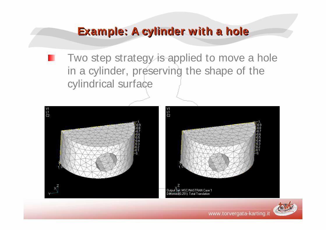
Example: A cylinder with a holeExample: A cylinder with a hole

Two step strategy is applied to move a hole in a cylinder, preserving the shape of the cylindrical surface

Documents

Dynamic mesh: beyond Fluent - Tor Vergata Kartingtorvergata-karting.it/...mesh_2007_Biancolini.pdf · Dynamic mesh: beyond FluentDynamic mesh: beyond Fluent Marco Evangelos Biancolini