Geospatial Analysis of High Risk Runoff Zones: Bailey’s Brook and Maidford

River Watersheds

By

Dustin Weisel

A MAJOR PAPER SUBMITTED IN PARTIAL FULFILLMENT OF THE REQUIREMENTS FOR THE

DEGREE OF MASTER OF ENVIRONMENTAL SCIENCE AND MANAGEMENT

UNIVERSITY OF RHODE ISLAND

April 25, 2015

MAJOR PAPER ADVISOR: Dr. Arthur Gold

MESM TRACK: Wetlands, Watersheds and Ecosystem Science

Abstract

Water quality throughout the Bailey’s Brook and Maidford River watersheds poses a problem to

potable drinking water reservoirs and coastal water quality on Aquidneck Island, Rhode Island. This

major paper focused on geospatial analyses to locate critical management zones that have a high risk of

generating and delivering pollutant loads to receiving waters. These locations represent areas worthy of

further consideration for water quality restoration practices. Critical management zones were identified

as the intersection of hydrologically sensitive areas that generate overland runoff with land use

locations areas with high potential for pollutant loading areas. Geospatial coverages of soil wetness,

runoff curve number and wetlands were produced to highlight hydrologically sensitive areas; while

developed land uses, such as agriculture, commercial and dense residential areas were identified as high

risk areas of pollutant generation. Critical management zones are an essential component of strategic

targeting that can promote efficient investments for water quality improvements. Maps and a

documented geospatial database for the two watersheds were produced and made available for future

use to highlight and locate these critical watershed management zones.

Introduction

Pollution from urban non-point sources is one of the main reasons that rivers and receiving

waters (e.g., lakes, reservoirs and estuaries) fail to reach their state and national water quality objectives

(Mitchell, 2004). Non-point source pollution often involves a plethora of pollutants including sediments,

nutrients, pesticides and pathogens (Walter et al., 2000). Although non-point pollution was initially

envisioned as difficult to locate, there has been an increasing recognition that advances in geospatial

data can provide insight into the combination of factors can create hotspots of nonpoint pollution.

These hotspots typically include zones that combine a high likelihood for offsite hydrologic transport

with elevated sources of pollutants. If these hotspots can be identified, they can provide a basis for

strategic protection and restoration efforts by local planners and water quality organizations. These

hotspots are also referred to as “Critical Management Zones” by various researchers (Figure 1; Walter et

al., 2000; Gburek et al., 2002).

Hydrologically Sensitive Areas (HSA) is saturated areas in a watershed that generate runoff

creating a potential transport for pollution into nearby waterways (Walter Et al., 2000). Hydrologically

Sensitive Areas are not a nonpoint pollution problem unless they coincide with a Pollutant Loading Area.

Some examples of Pollutant Loading Areas are agricultural fields, residential areas and commercial

properties. Increases in the percent agriculture and percent urban development throughout at

watershed are frequently associated with declining water quality, with increases in the surface water

concentrations of nitrogen, phosphorus and fecal coliform bacteria are related (Mehaffey, Et al., 2005) .

A key strategy for controlling nonpoint source pollution is to minimize the pollutant loading on a HAS

(Frankenberger, Et al., 1999). The management area to focus on is where the HSA and Pollutant Loading

Areas correspond as the Critical Management Area. Critical Management zones are found when field

boundaries (Pollutant Loading Area) are spatially overlaid by the saturation area (HSA). Identifying and

reducing offsite pollution from critical management areas within a watershed can be an efficient way to

minimize the amount of pollutants transported in surface runoff (Walter, et al., 2000).

Purpose

In this major paper, I will generate maps and geospatial databases of potential hot spots of

nonpoint pollution for two watersheds, Bailey’s Brook and the Maidford River, that contribute to the

drinking water reservoirs on Aquidneck Island, RI (Figure 2a and 2b – show a map with the watersheds

and the reservoirs). These reservoirs have degraded water quality and require advanced water

treatment to generate potable water for the Aquidneck Island residents (McLaughlin, 2014). I will use

land use to identify high-risk areas of pollution and combine those areas with analyses that predict

locations at high risk for overland runoff. These hotspot maps are intended to assist water quality

managers at the local and state level in their efforts to target restoration efforts in a strategic fashion

and thus reduce watershed pollution in a more cost efficient fashion.

Background

This paper is focused on the attributes of two watersheds Bailey’s Brook and Maidford River, in

Middletown, RI on Aquidneck Island that drain into drinking water reservoirs(North Easton Pond,

Gardiner and Nelson Ponds) that are deemed to be impaired due to issues with excessive nitrates and

bacteria (RIDEM a, 2013). Both of these watersheds are undergoing TMDL studies (McLaughlin, 2014).

Total Maximum Daily Load (TMDL) is a phrase that EPA and State’s use to reflect studies and programs

used to restore impaired waters. Formally, it represents the maximum daily input of a particular

pollutant that will not impair the functions and value of water body. The assumption is that if the

loading (i.e., input) of a pollutant increases over the TMDL, water quality issues will occur. TMDL studies

are now underway on these watersheds.

Bailey’s Brook is a 4.8-mile long stream with two flowing branches that join at North Easton

Pond. The southern flowing stream moves through North Easton Pond to South Easton Pond where it

empties into the Atlantic Ocean at Easton’s Beach. North Easton Pond is one of the key water supply

reservoirs serving Aquidneck Island residents. The Bailey’s Brook watershed cover approximately 3.1

square miles and is highly developed with 68% of the total watershed being built up; 32% of the area is

impervious cover (RIDEM a, 2013). Impervious cover is defined as land surface areas that force water to

runoff and not infiltrate into the soils, such as roofs and roads. Currently about 15% of the watershed is

agriculture, 12% is forested or non-developed, and 4% is covered with wetlands. Rhode Island Nursery

is the largest agricultural operation in the watershed. Based on Rhode Island DEM’s study, the nursery is

potentially important for putting phosphorus into Bailey’s Brook (RIDEM a, 2013). The soils of the

watershed are almost all classified as hydrologic group C by the USDA Natural Resource Conservation

Service SSURGO soil maps. Hydrologic C soils cause water to infiltrate slowly and have a hardpan layer

at 2-6 feet that restricts deep percolation and can cause periods of shallow water tables. Most of the

residents have sewers, but a few have septic systems that could fail and cause raw sewage to make its

way into Bailey’s Brook (RIDEMa, 2013).

The other watershed analyzed contains the 0.9-mile stream called the Maidford River. This

stream flows south through agricultural fields to Nelson and Gardiner Pond eventually emptying into the

ocean at Sachuest Beach on Sachuest Point. This is a small watershed that covers 3.5 square miles and

the main land use is agricultural at 39% (RIDEMb, 2013) Forested lands make up about 22% of the

watershed while developed land is 29% with impervious cover at 9%. The main sources of pollution in

the area are from agricultural activities, wildlife and domestic animal waste, storm water runoff from

the developed areas and illicit discharges (RIDEMb, 2013). With animals able to graze near the stream

and spreading manure as fertilizer, there are substantial amounts of bacterial contaminants leaching

into the river.

Figure 2b: The Maidford River watershed located in Middletown RI, on Aquidneck Island

Identifying Hotspots

High Risk Land Use/Land Cover Areas

Agricultural nutrient loading is expected to be high from annual cropland (e.g., silage

corn), confined animal zones (e.g., paddocks, barnyards), heavily grazed pastures and lands that are

plowed and heavily manured. Agricultural lands that are expected to generate lower pollution include

those in perennially crops such as hay lands, orchards or vineyards. Agriculture can be the major

contributor to concentrations of total nitrogen and total phosphorous in some stream systems

(Mehaffey Et al., 2004). Urban land use areas generate nutrients from domestic pet wastes (the majority

of the nutrient loss comes from urine, rather than feces; Mihelcic et al., 2011); sanity sewer leaks, failing

septic systems and landscape fertilization (Ahearn, et al., 2005). Investigators recognize that human

actions to the landscape are a threat to ecological integrity and water quality of a stream (Allan, 2004).

To identify locations that have the potential to generate elevated non-point pollution, I used the Land

Use- 2011 coverage from RIGIS. The following table includes those LU/LC classes identified as high risk:

Table 1: Land use-Land Cover codes with definitions and pollution risks.

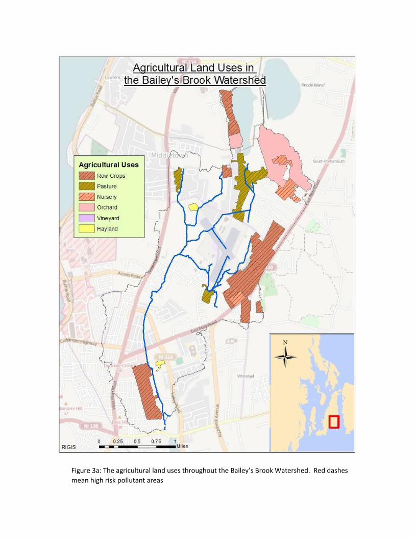
Figure 3a: The agricultural land uses throughout the Bailey’s Brook Watershed. Red dashes

mean high risk pollutant areas

Figure 3b: The agricultural land uses throughout the Maidford River Watershed. Red dashes

mean high risk pollutant areas.

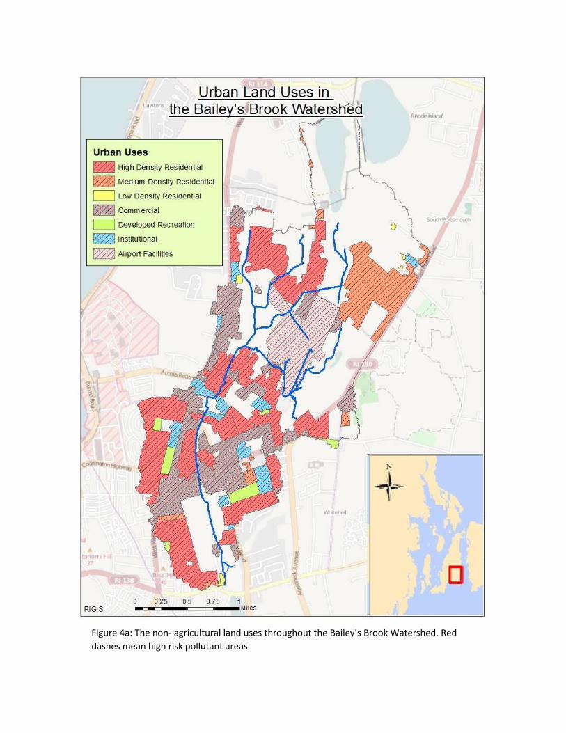
Figure 4a: The non- agricultural land uses throughout the Bailey’s Brook Watershed. Red

dashes mean high risk pollutant areas.

Figure 4b: The non-agricultural land uses throughout the Maidford River Watershed. Red

dashes mean high risk pollutant areas.

High Risk Runoff Locations (Hydrologically Sensitive Areas)

Variable Source Areas

One approach to identify locations with high runoff potential is termed Variable Source Area

Hydrology. Variable Source Area Hydrology is a risk assessment concept that assumes that saturated

areas are the primary source of runoff (Mehta, Et al., 2004). These locations are termed Hydrologically

Sensitive Areas (HSA) and during a storm, these saturated areas are the first to generate overland flow.

Runoff provides a quick transport mechanism for pollutants between the landscape and surface

waterbodies (Walter, et al., 2000).

The common areas for saturation to occur are in shallow soils above a restrictive layer, where

the downhill slope of a hill decreases or in topographically converging areas (Figure 5). HSAs become a

problem when their location coincides with areas of large pollutant loading such as row crop agriculture,

animal operations or septic systems. Figure 5 displays the flow of water on a slope with a restrictive

layer. During the storm, water infiltrates into the soil until it hits the restricting layer. This will cause

interflow down the slope. Interflow avoids the nutrients and pollutants caused from overland flow.

Areas with a thin layer of soil above the restricting layer will become saturated first (Labeled with a

Star). Overland flow will occur at the saturated areas on the slope, picking up nutrients, sediments or

pollutants as the water moves to the streams.

Figure 5: 1.) Shallow Soil, 2.) Convergence Area, 3.) Downhill Slope Decreases (Walter et. al, 2000)

Hydrologically Sensitive Areas are identified through geospatial analyses.

Enhanced topographic index

The enhanced topographic index (ETI) provides insight into the pattern and extent of runoff generating

areas within a watershed (Beven and Kirby 1979; Beven, 1986; Sivapalan et al., 1987). It is developed

by first “gridding” the watershed of interest into individual cells (i.e., rasters). For the analysis of the

Maidford and Bailey’s Brook watersheds a 30 x 30 m cell size was used (Figures 6a and 6b, referred to as

Soil Wetness). The ETI for each raster is then calculate from a ratio developed from topographic

attributes and soil transmissivity.

The topographic attributes include the topographic slope of each cell (referred to as “Tanb” ) and a flow accumulation component based on the number of upslope cells (i.e,. upslope area) that drain into each cell per unit length of contour (referred to as “a”).

Soil transmissivity is defined as saturated hydraulic conductivity (k; Length/time) times the depth of soil (d; length) above a restrictive layer. The SSURGO 1:24,000 dataset for RI was used to obtain soil transmissivity for each cell (i.e., referred as hydraulic conductivity per cell, ki, times depth per cell, di, resulting in a transmissivity value per cell of kidi). The soil transmissivity index value for each cell is then obtained from geometric mean of all the grid cells (avg dk) divided by the soil transmissivity of each cell (kidi).

ETI is then computed for each cell as:

ETI = ln(a/tanb)+ln((avg(dk)/(kidi))

One method of finding these areas is the Soil Moisture Routing Model (SMR). The SMR model is

a raster based analysis of the water balance at each time step for each cell of the watershed

(Frankenberg, Et al., 1999). SMR combines elevation, soil, and land use maps, six soil parameters, and

three daily weather parameters. This analysis provides flow throughout the watershed based on the

high saturation areas. Water balance is calculated for each cell in the model and runoff is generated

when the rainfall exceeds the storage capacity of the cell (Johnson et al., 2003). Soil moisture is a key

variable that largely influences rain becoming runoff or infiltrating into ground water (Aubert et al.,

2003). SMR is a water quality tool that effectively simulates variable source areas for rural watersheds

(Johnson et al., 2003).

Figure 6a: Pattern of overland runoff generating areas based on the Enhanced Topographic Index for the

Bailey’s Brook Watershed.

Figure 6b: Pattern of overland runoff generating areas based on the Enhanced Topographic Index for the

Maidford River Watershed.

NRCS CURVE NUMBERS

Soil hydrologic group data can be combined with land use data to identify high-risk runoff area is

through the NRCS Curve-Number Method (Patil et al., 2008). Hydrologic soil groups are created based

on the composition of the soil and the potential runoff when thoroughly wet. The Bailey’s Brook and

Maidford watersheds have an abundance of hydrologic soil group C soils. This type of soil has

moderately high runoff potential when the soil is wet. Curve numbers are based on the land cover,

hydrologic condition (e.g., is the land cover compacted from human or animal activities) and the

hydrologic soil groups.

Soil geospatial soil data collected by the National Cooperative Soil Survey classifies the

hydrologic soil group for each soil map unit (Table 2). Soil geospatial data are available at coarse scales

(e.g., 1:100,000) through STATSGO and at finer resolutions (e.g., 1:20,000) through SSURGO. Areas with

higher curve numbers are predicted to generate more runoff for a given 24-hour rainstorm than areas

with lower curve numbers.

Table 3 is the chart of curve numbers for urban areas and the hydrologic soil groups. The chart

shows that the curve number for an open space with poor conditions is 86; while the curve number for a

Table 2: NRCS Hydrologic Soil Groups with definitions and examples

parking lot is 98 even though they still have the same hydrologic soil group (C). Once the curve numbers

are known, they can be put into the curve number graph (figure8) to find the amount of runoff. The

curve numbers in the example are analyzing a 5-inch storm. Find on the X-axis the amount of rain that

has fallen (Blue Line). Then move up that line to the curve with the number that corresponds to the

area of interest. From that curve, move over to the Y-axis to see the amount of runoff that has

occurred. The graph shows that a C hydrologic soil group with a curve number of 98 (Red Line) and 86

(Green Line) has almost a two inch difference based on the same storm event. The more runoff from an

area will have a shorter time that the streams are flooded; this is known as the Time of Concentration.

A shorter time of concentration can cause extreme floods causing erosion, sedimentation and pollution

in the stream.

Table 3: Runoff Curve-Numbers for Urban Areas.

Figure 7: Depth of direct overland runoff based off the amount of rainfall

over a 24-hour period and the curve-number. The examples display the

depth of runoff predicted for a 5-inch 24-hour storm.

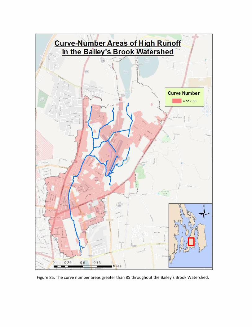
Figure 8a: The curve number areas greater than 85 throughout the Bailey’s Brook Watershed.

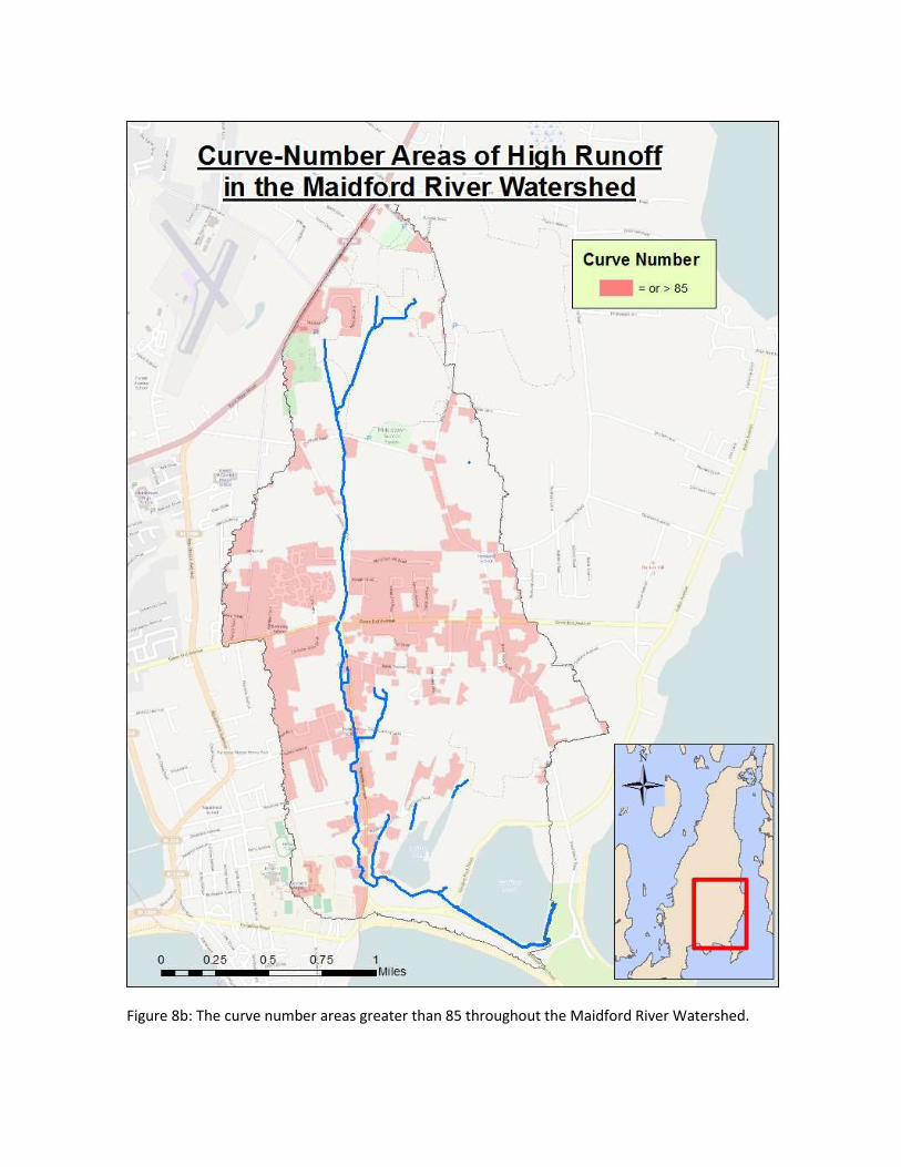
Figure 8b: The curve number areas greater than 85 throughout the Maidford River Watershed.

Wetlands

Wetlands are lands that experience extended periods of saturation (Strecker et al., 2001).

Although Wetlands reduce peak flow rates (i.e., the extent of flooding) by slowing the rate of overland

runoff. However, wetlands have limited capacity to absorb rainwater and are often spots where

overland runoff is generated through a process known as direct precipitation on saturated areas (Dunne

and Leopold, 1978). Wetlands can function as a water quality enhancer in the denitrification process,

nutrient processing and in flood abatement (Moore et al., 2002). These saturated areas are the most

fragile parts of the landscape due to the rapid storm flow runoff produced by them during a storm

(O’Loughlin, 1981). Wetlands are integral parts to the landscape and human values (Mitsch and

Gosselink, 2000), but for our research analyzing the Bailey’s Brook and the Maidford River Watershed,

saturated areas are considered HAS – zones with high risks for generating overland runoff and

contribute to creation of the critical management areas if they are adjacent to sources of pollution

generation. Based on land use, more runoff and pollutants enter the wetland causing ecological damage

to the system (Zedler, 2003). Agriculture fields discharge large amounts of nutrients that are

threatening the wetland plant species and creating nutrient loading in the nearby streams.

Wetland Codes Description

Inland (Freshwater)

1-ROW Riverine Non-tidal Open Water

2-LOW Lacustrine Open Water

3-POW Palustrine Open Water

4-EMA Emergent Wetland: Marsh/Wet Meadow

5-EMB Emergent Wetland: Emergent Fen or Bog

6-SSA Scrub Shrub Swamp

7-SSB Scrub Shrub Wetland: Shrub Fen or Bog

8-FOA Forested Wetland: Coniferous

9-FOB Forested Wetland: Deciduous

10-FOD Forested Wetland: Dead

Coastal (Saltwater)

11-RTW Riverine Tidal Open Water

12-EOW Estuarine Open Water

13-ERS Marine/Estuarine Rocky Shore

14-EUS Marine/Estuarine Unconsolidated Shore

15-EEM Estuarine Emergent Wetland

16- ESS Estuarine Scrub-Shrub Wetland

99- UPL Upland

Table 4: Wetland codes with a description.

Figure 9a: The wetlands throughout the Bailey’s Brook Watershed.

Figure 9b: The wetlands throughout the Maidford River Watershed.

Critical Management Zones

Critical Management Areas are created by the confluence of hydrological sensitive areas with

certain types of agricultural lands (referred to as high intensity). Vineyards and orchards are not

considered to be major pollutant loading areas and are thus excluded from depictions of the critical

management areas. In this study hydrological sensitive areas are defined through a number of

geospatial attributes, including soil hydrologic groups C or D; wetlands and lands with elevated curve

numbers (>85).

Figures 11a and 11b depicts the total area of critical management areas due to high intensity

agriculture in the Bailey’s Brook and Maidford River watersheds using different attributes to define

Hydrological Sensitive Areas.

Wetlands near Agricultural Lands

Wetlands are extremely saturated areas that have a high potential runoff chance. Wetlands

receiving fertilized field runoff experience major shifts in nutrient concentration and variable hydrologic

loading (Poe et al. 2003). Some services that wetlands provide are flood abatement, improved water

quality and help support biodiversity (Zedler, 2003).

Figure 10a: The HSAs defined as a CN greater than 85 and wetlands throughout the Bailey’s

Brook watershed.

Figure 10b: The HSAs defined as a CN greater than 85 and wetlands throughout the Maidford

River watershed.

Figure 11a. Possible Critical Management Zones within the Bailey’s Brook Watershed. These areas are likely to be an overestimate and will likely be refined through field work that identifies the types of agricultural practices and urban stormwater best management practices associated with specific parcels.

Figure 11b. Possible Critical Management Zones within the Maidford River Watershed.

These areas are likely to be an overestimate and will likely be refined through field work

that identifies the types of agricultural practices and urban stormwater best management

practices associated with specific parcels.

Future Work

This study was to create maps and perform an analysis for critical management zones (CMZs) of

the Bailey’s Brook and Maidford River watersheds in Middletown, RI. Our CMZs were defined as the

areas with a curve number greater than 85 or with a wetland. The critical management zones are areas

that are in need of improvement within the watersheds. From the results of Figures 11a and 11b, it can

be observed that both watersheds have substantially high amounts of critical management zones. High

amounts of CMZs can lead to large amounts of pollutants running off into the nearby streams.

Further work is required to refine the critical management zones in each watershed. The

agricultural crops and practices employed on each parcel should be identified and the risk of pollutant

loading should be reevaluated based on those data. Urban parcels should be examined for stormwater

best management practices. Where suitable practices are in place, those parcels should be reclassified

as low risk.

Finally, I suggest that the Enhanced Topographic Indices that display the likelihood of overland

runoff generation (Figures 6a and 6b) be used as another geospatial coverage to identify hydrologic

sensitive areas. These indices can help target management practices to pollutant loading areas that

overlie areas that produce concentrated overland flow.

Acknowledgements

I would like to thank Art Gold for reviewing my paper and maps throughout the research

process. AIso, thank you to Professor Soni Pradhnang for giving me the steps to create a soil wetness

and land use curve number maps for this paper.

Figure 12b: The HSAs dispersed throughout the non- agricultural land uses of Maidford

River Watershed.

APPENDIX A: Creating Soil Wetness Map

Soil Transmissivity (Wetness)

1. Obtain SSURGO2 layer for your site.

2. Download soil data viewer tool and add to the ArcGIS

3. Use soil data viewer to extract depth to restrictive layer(desoil) and hydraulic conductivity

layers (ksat) (average area weighted) [Make sure Ksat values are converted to cm/day)

4. Multiply grids [desoil] and [ksat] and 1000 (to get soil depth and hydraulic conductivity product

grid in sq. m per day) using raster calculator in spatial analyst tool; grid name: ZKsat

5. Obtain geometric mean value of this product (ZKsat), for example 11248.841

6. Divide ZKsat grid by mean value , i.e., 11248.841/[ZKsat] using raster calculator

1. Finally use raster calculator to calculate soil transmissivity value. [Spatial Analyst—Raster

Calculator[ log((avg(dk)/(DiKi))--Evaluate] ; grid name: lnZKsat

APPENDIX B: Assigning Curve Numbers to Land use map

Calculating Curve Numbers Using GIS

The Hydrologic Studies Unit (HSU) of Michigan’s Department of Environmental Quality (MDEQ)

has developed a method to compute curve numbers from GIS land use and soils information.

The instructions assume that you have an ArcView project open with a delineated watershed

theme, land use theme, and a soils theme.

The basic technique is to assign a number less than 100 to each land use category and a

number that is a multiple of 100 to each soil category. The two numbers are summed. Curve

numbers are associated with each summed number. A composite curve number is then

calculated using area-weighted averaging. Specific instructions are as follows.

In these instructions, italics are used to highlight ArcView menu items and variables. Bold is used to

highlight Field names in tables.

Works Cited Ahearn, Dylan S., Richard W. Sheibley, Randy A. Dahlgren, Michael Anderson, Joshua Johnson, and Kenneth W. Tate. "Land Use and Land Cover Influence on Water Quality in the Last Free-flowing River Draining the Western Sierra Nevada, California." Journal of Hydrology 313.3-4 (2005): 234-47. Print. Allan, J. David. "Land Scapes of Riverscapes: The Influence of Land Use on Stream Ecosystems." Annual Review of Ecology, Evolution and Systematics 35 (2004): 257-84. Print. B, RIDEM. "Maidford River." RIDEM (2013): 1-13. Print.

Beven, K J. 1986 Runoff production and flood frequency in catchments of order n: an alternative approach, in: Scale Problems in Hydrology, edited by: Gupta, V. K., Rodriguez-Iturbe, I., and Wood, E. F., Reidel, Dordrecht, 107–131.

Beven, K. J. and Kirkby, M. J. 1979. A physically based, variable con- tributing area model of basin hydrology, Hydrol. Sci. J. 24: 43– 69,

Dunne, T. and Leopold, L.B., 1978. Water in Environmental Planning. Freeman, San Francisco, CA, 818 pp

Gburek, W. J., C. C. Drungil, M. S. Srinivasan, B. A. Needelman, and D. E. Woodwork. "Variable Source Area Controls on Phosphorus Transport; Bridging TheGap between Research and Design." Journal of Soil and Water Conservation 57.6 (2002): 534-43. Print. McLaughlin, Dave. "Clean Ocean Access 2008-2013 Water Quality Monitoring Sumary Report." Clean OCean Access (2014): 1-48. Print. Mehaffey, M. H., M. S. Nash, T. G. Wade, and D. W. Ebert. "Linking Land Cover and Water Quality in New York City's Water Supply Watersheds." Environmental Monitoring and Assessment 107 (2005): 29-44. Print. Mehta, Vishal K., M. Todd Walter, Erin S. Brooks, and Micheal F. Walter. "Application of SMR to Modeling Watersheds in the Catskill Mountains." Environmental Modeling and Assessment 9 (2004): 77-89. Print. Mihelcic, James R., Lauren M. Fry, and Ryan Shaw. "Global Potential of Phosphorus Recovery from Human Urine and Feces." Chemosphere 84.6 (2011): 832-39. Print. Mitchell, Gordon. "Mapping Hazard from Urban Non-point Pollution: A Screening Model to Support Sustainable Urban Drainage Planning." Journal of Environmental Management 74 (2005): 1-9. Print. Mitsch, William J., and James G. Gosselink. "The Value of Wetlands: Importance of Scale and Landscape Setting." Ecological Economics 35.1 (2000): 25-33. Print. Moore, M. T., R. Shulz, C. M. Cooper, S. Smith, Jr., and J. H. Rodgers, Jr. "Mitigation of Chlorpyrifos Runoff Using Constructed Wetlands." Chemosphere 46 (2002): 827-35.

O'loughlin, E. M. "Saturation Regions in Catchments and Their Relations to Soil and Topographic Properties." Journal of Hydrology 53 (1981): 229-46. Print. Patil, J.p., A. Sarangi, A.k. Singh, and T. Ahmad. "Evaluation of Modified CN Methods for Watershed Runoff Estimation Using a GIS-based Interface." Biosystems Engineering 100.1 (2008): 137-46. Print. Poe, Amy C., Micheal F. Piehler, Suzanne P. Thompson, and Hans W. Paerl. "Denitrification in a Construced Wetland Receiving Agricultural Runoff." Wetlands 23.4 (2003): 817-26. Print. A, RIDEM. "Bailey's Brook." RIDEM (2013): 1-13. Print. Rogers, G.O., B.B. Defee. “Long-Term Impact of Development on a Watershed: Early Indicators of Future Problems.” Landscape and Urban Planning 73 2005: 215-233.

Sivapalan, M., K. Beven and E.F. Wood. 1987. “On hydrologic similarity. 2. A scaled model of storm runoff production,” Water Resources Research. 23:2266-2278.

Strecker, Eric W., Marcus M. Quigley, Ben R. Urbonas, Jonathan E. Jones, and Jane K. Clary. "Determining Urban Storm Water BMP Effectiveness." Journal of Water Resources Planning and Management 127.3 (2001): 144-49. Print. Walter, M. T., M. F. Walter, E. S. Brooks, and T. S. Steenhuis. "Hydrologically Sensitive Areas: Variabe Source Area Hydrology Implications for Water Quality Risk Assessment." Journal of Soil and Water Conservation 55.3 (2000): 277-84. Print. Zedler, Joy B. "Wetlands at Your Service: Reducing Impacts of Agriculture at the Watershed Scale." Frontiers in Ecology and the Environment 1.2 (2003): 65. Print.